Embed Size (px)
Citation preview

UNIVERSIDADE FEDERAL DO RIO GRANDE DO SULINSTITUTO DE INFORMÁTICA
PROGRAMA DE PÓS-GRADUAÇÃO EM COMPUTAÇÃO
MILTON ROBERTO HEINEN
A Connectionist Approach for IncrementalFunction Approximation and On-line Tasks
Thesis presented in partial fulfillmentof the requirements for the degree ofDoctor of Computer Science
Prof. Dr. Paulo Martins EngelAdvisor
Porto Alegre, March 2011

CIP – CATALOGING-IN-PUBLICATION
Heinen, Milton Roberto
A Connectionist Approach for Incremental Function Approx-imation and On-line Tasks / Milton Roberto Heinen. – Porto Ale-gre: PPGC da UFRGS, 2011.
172 f.: il.
Thesis (Ph.D.) – Universidade Federal do Rio Grande do Sul.Programa de Pós-Graduação em Computação, Porto Alegre, BR–RS, 2011. Advisor: Paulo Martins Engel.
1. Machine learning. 2. Artificial neural networks. 3. Incre-mental learning. 4. Bayesian methods. 5. Gaussian mixture mod-els. 6. Function approximation. 7. Regression. 8. Clustering.9. Reinforcement learning. 10. Autonomous mobile robots. I. En-gel, Paulo Martins. II. Título.
UNIVERSIDADE FEDERAL DO RIO GRANDE DO SULReitor: Prof. Carlos Alexandre NettoVice-Reitor: Prof. Rui Vicente OppermannPró-Reitor de Pós-Graduação: Prof. Aldo Bolten LucionDiretor do Instituto de Informática: Prof. Flávio Rech WagnerCoordenador do PPGC: Prof. Álvaro Freitas MoreiraBibliotecária-chefe do Instituto de Informática: Beatriz Regina Bastos Haro

“I do not know what I may appear to the world, but to myself I seem tohave been only like a boy playing on the sea-shore, and diverting myself
in now and then finding a smoother pebble or a prettier shell than ordinary,whilst the great ocean of truth lay all undiscovered before me.”
— SIR ISAAC NEWTON
“Any intelligent fool can make things bigger, more complex,and more violent. It takes a touch of genius – and a lot of
courage – to move in the opposite direction.”“I have no special talent. I am only passionately curious.”
— ALBERT EINSTEIN
“Intelligence is the ability to adapt to change.”— STEPHEN HAWKING


ACKNOWLEDGEMENTS
I am grateful to my advisor, Dr. Paulo Martins Engel, for the ideas that led to this the-sis, for his guidance, encouragement, valuable comments, support and patience through-out the course of this work. I thank the professors and teachers of the Informatics Institute,for transmitting the knowledge necessary to accomplish this journey, and to Dr. FernandoSantos Osório, for his continuing support and valuable advice. Another great debt is tomy colleagues of the Neural Networks group for discussions, comments, and support.Thanks to Edson Prestes for lending us his Pioneer 3-DX robot which was used in someexperiments. I also acknowledge the financial support granted by CNPq.
Finally I would like to acknowledge my thanks to my family. My parents, Arno JoséHeinen and Melânia Heinen, supported me with their encouragement and comprehension.My dearest lovely wife, Alessandra Hüther Heinen, provided me constant support whichhelped me to overcome many difficulties on the way to completing this journey.
I dedicate this work to my dearest lovely wife, Alessandra Hüther Heinen, who duringall these years has always been by my side, especially when I most needed her support,fondness and love.


CONTENTS
LIST OF ABBREVIATIONS AND ACRONYMS . . . . . . . . . . . . . . . . 9
LIST OF SYMBOLS . . . . . . . . . . . . . . . . . . . . . . . . . . . . . . . 11
LIST OF FIGURES . . . . . . . . . . . . . . . . . . . . . . . . . . . . . . . . 15
LIST OF TABLES . . . . . . . . . . . . . . . . . . . . . . . . . . . . . . . . 17
ABSTRACT . . . . . . . . . . . . . . . . . . . . . . . . . . . . . . . . . . . 19
RESUMO . . . . . . . . . . . . . . . . . . . . . . . . . . . . . . . . . . . . . 21
1 INTRODUCTION . . . . . . . . . . . . . . . . . . . . . . . . . . . . . . 231.1 Function approximation . . . . . . . . . . . . . . . . . . . . . . . . . . . 251.2 Theoretical and biological inspiration . . . . . . . . . . . . . . . . . . . 261.3 Main objectives and contributions of this thesis . . . . . . . . . . . . . . 301.4 Outline . . . . . . . . . . . . . . . . . . . . . . . . . . . . . . . . . . . . 31
2 GAUSSIAN MIXTURE MODELS . . . . . . . . . . . . . . . . . . . . . . 332.1 Gaussian mixture models . . . . . . . . . . . . . . . . . . . . . . . . . . 332.2 K-means clustering algorithm . . . . . . . . . . . . . . . . . . . . . . . . 342.3 The EM algorithm . . . . . . . . . . . . . . . . . . . . . . . . . . . . . . 352.4 State-of-the-art about learning Gaussian mixture models . . . . . . . . . 362.5 Incremental Gaussian Mixture Model . . . . . . . . . . . . . . . . . . . 402.5.1 Tackling the Stability-Plasticity Dilemma . . . . . . . . . . . . . . . . . 412.5.2 Model update by sequential assimilation of data points . . . . . . . . . . 422.5.3 Creating a new component based on novelty and stability . . . . . . . . . 472.5.4 Incremental learning from unbounded data streams . . . . . . . . . . . . 482.5.5 IGMM learning algorithm . . . . . . . . . . . . . . . . . . . . . . . . . . 492.5.6 Computational complexity of IGMM . . . . . . . . . . . . . . . . . . . . 502.6 Comparative . . . . . . . . . . . . . . . . . . . . . . . . . . . . . . . . . 51
3 ARTIFICIAL NEURAL NETWORKS . . . . . . . . . . . . . . . . . . . . 533.1 Multi-layer Perceptrons . . . . . . . . . . . . . . . . . . . . . . . . . . . 533.2 Radial basis function networks . . . . . . . . . . . . . . . . . . . . . . . 543.3 Self-organizing maps . . . . . . . . . . . . . . . . . . . . . . . . . . . . . 553.4 Adaptive Resonance Theory . . . . . . . . . . . . . . . . . . . . . . . . . 563.5 ARTMAP . . . . . . . . . . . . . . . . . . . . . . . . . . . . . . . . . . . 593.6 Probabilistic neural networks . . . . . . . . . . . . . . . . . . . . . . . . 61

3.7 General regression neural network . . . . . . . . . . . . . . . . . . . . . 633.8 Improvements made over PNN and GRNN . . . . . . . . . . . . . . . . 653.9 Other neural network models . . . . . . . . . . . . . . . . . . . . . . . . 693.10 Comparison among the described ANN models . . . . . . . . . . . . . . 70
4 INCREMENTAL GAUSSIAN MIXTURE NETWORK . . . . . . . . . . . 734.1 General regression using Gaussian mixture models . . . . . . . . . . . . 734.2 IGMN architecture . . . . . . . . . . . . . . . . . . . . . . . . . . . . . . 764.3 IGMN operation . . . . . . . . . . . . . . . . . . . . . . . . . . . . . . . 784.3.1 Learning mode . . . . . . . . . . . . . . . . . . . . . . . . . . . . . . . 794.3.2 Recalling mode . . . . . . . . . . . . . . . . . . . . . . . . . . . . . . . 824.4 Dealing with multi-valued target data . . . . . . . . . . . . . . . . . . . 844.5 IGMN configuration parameters . . . . . . . . . . . . . . . . . . . . . . 884.6 Final remarks . . . . . . . . . . . . . . . . . . . . . . . . . . . . . . . . . 88
5 FUNCTION APPROXIMATION USING IGMN . . . . . . . . . . . . . . 915.1 Sinusoidal data set . . . . . . . . . . . . . . . . . . . . . . . . . . . . . . 915.1.1 Standard × multivariate representation . . . . . . . . . . . . . . . . . . . 925.1.2 Assessing the sensibility of the δ parameter . . . . . . . . . . . . . . . . 965.1.3 Ordered × shuffled data sets . . . . . . . . . . . . . . . . . . . . . . . . 965.1.4 Estimating the confidence intervals . . . . . . . . . . . . . . . . . . . . . 1005.1.5 Comparison with other ANN models . . . . . . . . . . . . . . . . . . . . 1015.2 Approximating the “Mexican hat” function . . . . . . . . . . . . . . . . 1025.3 Estimating both a and b . . . . . . . . . . . . . . . . . . . . . . . . . . . 1045.4 Estimating the outputs of a nonlinear plant . . . . . . . . . . . . . . . . 1095.5 Predicting future values of a time series . . . . . . . . . . . . . . . . . . 1125.6 Final remarks . . . . . . . . . . . . . . . . . . . . . . . . . . . . . . . . . 116
6 ROBOTICS AN OTHER RELATED TASKS . . . . . . . . . . . . . . . . 1196.1 Incremental concept formation . . . . . . . . . . . . . . . . . . . . . . . 1196.1.1 Related work . . . . . . . . . . . . . . . . . . . . . . . . . . . . . . . . 1206.1.2 Concept formation experiments . . . . . . . . . . . . . . . . . . . . . . . 1226.2 Estimating the desired speeds in a mobile robotics application . . . . . . 1246.3 Computing the inverse kinematics in a legged robot task . . . . . . . . . 1286.4 Reinforcement Learning using IGMN . . . . . . . . . . . . . . . . . . . 1306.4.1 Related work . . . . . . . . . . . . . . . . . . . . . . . . . . . . . . . . 1316.4.2 Selecting the robot actions using IGMN . . . . . . . . . . . . . . . . . . 1316.4.3 Pendulum with limited torque . . . . . . . . . . . . . . . . . . . . . . . . 1326.4.4 Robot soccer task . . . . . . . . . . . . . . . . . . . . . . . . . . . . . . 1336.5 Feature-based mapping using IGMN . . . . . . . . . . . . . . . . . . . . 1356.5.1 Related work . . . . . . . . . . . . . . . . . . . . . . . . . . . . . . . . 1366.5.2 Incremental feature-based mapping using IGMN . . . . . . . . . . . . . . 1376.5.3 Experiments . . . . . . . . . . . . . . . . . . . . . . . . . . . . . . . . . 140
7 CONCLUSION AND FUTURE WORK . . . . . . . . . . . . . . . . . . 1477.1 Future work . . . . . . . . . . . . . . . . . . . . . . . . . . . . . . . . . . 149
REFERENCES . . . . . . . . . . . . . . . . . . . . . . . . . . . . . . . . . . 151
APPENDIX – PRINCIPAIS CONTRIBUIÇÕES DA TESE . . . . . . . . . . 169

LIST OF ABBREVIATIONS AND ACRONYMS
AI Artificial Intelligence
AMNN Attentional Mode Neural Network
ANN Artificial Neural Network
ARAVQ Adaptive Resource Allocating Vector Quantization
ART Adaptive Resonance Theory
ARTMAP Predictive ART
BP Back-Propagation
DDA Dynamic Decay Adjustment
EM Expectation-Maximization
FPGA Field Programmable Gate Array
FPNN Fuzzy Probabilistic Neural Network
GA Genetic Algorithm
GC Gaussian Clustering
GF Generalized Fisher
GMM Gaussian Mixture Model
GRNN General Regression Neural Network
GTSOM Growing Temporal Self Organizing Map
HMM Hidden Markov Models
IGMM Incremental Gaussian Mixture Model
IGMN Incremental Gaussian Mixture Network
INBC Incremental Naïve Bayes Clustering
IPNN Incremental Probabilistic Neural Network
LMS Least Mean Squares
LWR Locally Weighted Regression
MDL Minimum Description Length
ML Maximum Likelihood

MLP Multi-Layer Perceptron
MPF Memory Prediction Framework
MSE Mean Square Error
NN Neural Network
NRMS Normalized Root Mean Squared
ODE Open Dynamics Engine
pdf Probability density function
PDBNN Probabilistic Decision-Based Neural Network
PNN Probabilistic Neural Network
RAN Resource Allocating Network
RBF Radial Basis Function
RL Reinforcement Learning
RMS Root Mean Squared
R-LLGMN Recurrent Log-Linearized Gaussian Mixture Network
SLAM Simultaneous Localization and Mapping
SOM Self-Organizing Maps
VB Variational Bayes
WPNN Weighted Probabilistic Neural Network

LIST OF SYMBOLS
a Sensory/motor stimulus of the first cortical region
b Sensory/motor stimulus of the second cortical region
〈b|a〉 Regression of b conditioned on a
C Variance/covariance matrix
Cj Complete jth covariance matrix of z
CAAj Submatrix containing the rows and columns of A in Cj
CABj Submatrix containing the rows corresponding to A and the columns
corresponding to B in Cj
CBAj Association matrix: CBA
j = CABjT
CBAj∗ New (updated) association matrix
CBBj Submatrix containing the rows and columns of B in Cj
CKj Covariance matrix of the jth unit of region N K
CKj
∗ New (updated) covariance matrix j of region N K
CK Estimated covariance matrix of b
D Dimensionality of z
DK Dimensionality of the sensory/motor stimulus k
DM (·) Mahalanobis distance
Elg Discrepancies between the local and global models
e Euler number: e = 2.718281828
f(·) Forward function
f(·)−1 Inverse function
I Identity matrix
j Current Gaussian distribution
K Data sequence of N input vectors: K = k1, . . . ,kn, . . . ,kN
K Sample space of K
k Sensory/motor stimulus of the kth cortical region

k Estimate of the sensory/motor stimulus k
L(θ) Likelihood of θ for a given K
M Number of Gaussian units
M∗ New (updated) number of Gaussian units
N Number of training patterns
N A First cortical region of IGMN
N B Second cortical region of IGMN
N K kth cortical region of IGMN
N S Last cortical region of IGMN
N (k|µ,C) Multivariate Gaussian distribution
n Current training pattern
P Associative region
p(a,b) Joint density
p(a,b) Estimate of p(a,b)
p(b|a) Conditional density
p(j) A priori probability of jth Gaussian unit
p(j)∗ New (updated) a priori probability of jth Gaussian unit
p(j|a,b, . . . , s) Joint posterior probability: p(j|a,b, . . . , s) = p(j|z)
p(j|k) Posterior probability of k have been generated from j
p(k|j) Probability density function
p(k|j, `) Probability density function of the jth non-discarded component
p(k|θ) Component density function
p(`|a) Probability of the Maximum likelihood (ML) hypothesis `
Qmax Maximum Q value currently stored in the Gaussian units
Q(s, a) Value of the state-action pair (s, a)
s Sensory/motor stimulus of the last cortical region
spj Accumulator of the a posteriori probabilities of the jth unit
sp∗j New (updated) jth accumulator of the a posteriori probabilities
spmax Configuration parameter used to set maximum value of sp
spmin Configuration parameter used to identify spurious components
t Current time step
V (s) Value of the state s
xKj xK
j = µBj + CBA
j CAAj−1
(a− µAj )
(x, y, φ) Pose of a robotic actuator

z Combination of all sensory/motor stimuli: z = a,b, . . . , s
αmax Maximum difference between the orientations of equivalent clusters
αmin Minimum angle between the sensor bean and the cluster orientation
β Configuration parameter used to restart the sp accumulators
γ Configuration parameter used to restart the sp accumulators
δ Configuration parameter used to set the initial radius of the Gaussianunits
ε Independent Gaussian noise vector
ε Instantaneous normalized approximation error
εmax Configuration parameter used to set maximum approximation error
ηmax Maximum Mahalanobis distance between equivalent clusters
θ Set of parameters of the GMM: θ = (θ1, . . . , θj, . . . , θM)T
θj Set of parameters of the jth Gaussian distribution: θj = µj,Cj, p(j)
µ Mean
µKj Mean vector of the jth unit of region N K
µKj
∗ New (updated) mean vector j of the cortical region N K
µε Mean of ε
ρj Density of the jth cluster
ρmin Minimum cluster density (used to verify if a cluster is spurious)
σ Standard deviation or spreading parameter of GRNN
σ2 Variance
σini Initial radius of the covariance matrices
σKj Vector containing the jth standard deviation of k
σ2K Estimated variance of k
σε Standard deviation of ε
τnov Configuration parameter used to set the minimum likelihood criterion
υj Age of the Gaussian unit j
υmin Configuration parameter used to set the minimum age
Ω Configuration parameter used to discard secondary branches
ωj ωj = p(j|zt)/sp∗j` Maximum likelihood (ML) hypothesis
0 Zero matrix
∗ Subscript that indicate the new (updated) parameters


LIST OF FIGURES
Figure 1.1: Information flow in traditional connectionist models that follows theinformation system metaphor . . . . . . . . . . . . . . . . . . . . . . 27
Figure 1.2: Information flow in embodied systems: there is a closed loop of in-formation between perception and action . . . . . . . . . . . . . . . 28
Figure 1.3: Information flows up and down sensory hierarchies to form predic-tions and create a unified sensory experience . . . . . . . . . . . . . 29
Figure 3.1: Typical architecture of ART1 . . . . . . . . . . . . . . . . . . . . . . 57Figure 3.2: ARTMAP architecture . . . . . . . . . . . . . . . . . . . . . . . . . 60Figure 3.3: PNN for classification of patterns in two categories . . . . . . . . . . 62Figure 3.4: Architecture of the GRNN model . . . . . . . . . . . . . . . . . . . 64
Figure 4.1: IGMN architecture . . . . . . . . . . . . . . . . . . . . . . . . . . . 77Figure 4.2: Information flow through the neural network during learning . . . . . 80Figure 4.3: Information flow in IGMN during recalling . . . . . . . . . . . . . . 83Figure 4.4: A typical inverse problem in which the target data are multi-valued . 86
Figure 5.1: Sinusoidal data set of size N = 1000 corrupted with Gaussian noise . 92Figure 5.2: Experiments performed over the sinusoidal data set using εmax = 0.075 94Figure 5.3: Experiments performed over the sinusoidal data set using εmax = 0.025 94Figure 5.4: Comparison between standard and multivariate regression . . . . . . 95Figure 5.5: Assessing the sensibility of δ – Standard IGMN algorithm . . . . . . 97Figure 5.6: Assessing the sensibility of δ – Multivariate IGMN algorithm . . . . 97Figure 5.7: Ordered × shuffled data sets – Standard algorithm . . . . . . . . . . 98Figure 5.8: Ordered × shuffled data sets – Multivariate algorithm . . . . . . . . . 98Figure 5.9: Gaussian units added during learning – Multivariate algorithm . . . . 99Figure 5.10: Gaussian units added during learning – Standard algorithm . . . . . . 100Figure 5.11: Confidence estimates computed by IGMN over the sinusoidal data set 100Figure 5.12: Comparative of the NRMS error among ANNs – sinusoidal data set . 102Figure 5.13: Approximating the “Mexican hat” function using IGMN . . . . . . . 103Figure 5.14: Hyperbolic tangent data set corrupted with noise . . . . . . . . . . . 105Figure 5.15: Estimating both a and b in a hyperbolic tangent data set . . . . . . . 105Figure 5.16: Experiments performed over the cubic data set . . . . . . . . . . . . 106Figure 5.17: Estimating both a from b in the cubic data set . . . . . . . . . . . . . 106Figure 5.18: Circular data set used to evaluate IGMN using multiple hypothesis . . 107Figure 5.19: Estimating both a and b on the circular data set . . . . . . . . . . . . 108Figure 5.20: Returning multiple solutions for the circular data set . . . . . . . . . 108Figure 5.21: Identification models . . . . . . . . . . . . . . . . . . . . . . . . . . 109

Figure 5.22: Identification of the nonlinear plant using some previous approaches . 110Figure 5.23: Identification of a nonlinear plant using 1000 training samples . . . . 111Figure 5.24: Assessing the sensibility of IGMN to the εmax parameter . . . . . . . 111Figure 5.25: Assessing the sensibility of IGMN to the δ parameter . . . . . . . . . 112Figure 5.26: Predicting a time series using MLP . . . . . . . . . . . . . . . . . . 114Figure 5.27: Predicting the time series using Camargo’s model . . . . . . . . . . . 115Figure 5.28: Predicting the time series using IGMN . . . . . . . . . . . . . . . . . 115Figure 5.29: Predicting the time series using GRNN (σ = 0.075) . . . . . . . . . . 116Figure 5.30: 95% confidence intervals computed by IGMN . . . . . . . . . . . . . 117
Figure 6.1: Results obtained using the Nolfi and Tani’s model in an environmentcomposed by two rooms joined by a short corridor . . . . . . . . . . 121
Figure 6.2: Results obtained using ARAVQ in an environment composed by tworooms joined by a short corridor . . . . . . . . . . . . . . . . . . . . 122
Figure 6.3: Pioneer 3-DX robot with eight sonars and a differential steering drive 122Figure 6.4: Segmentation obtained by IGMN in six corridors experiment . . . . . 123Figure 6.5: Segmentation obtained by IGMN in the two rooms experiment . . . . 124Figure 6.6: Difference between the speeds of the right and left motors of the robot
while it is fallowing the trajectory shown in Figure 6.5. . . . . . . . . 125Figure 6.7: Trajectory obtained using IGMN to choose the robot actions . . . . . 126Figure 6.8: Comparing the approximation errors in the trajectory of Figure 6.5 . . 127Figure 6.9: Wall following behavior in a more complex environment. The solid
gray line shows the trajectory followed by the robot in the learningmode and the dashed black line shows the trajectory followed by therobot using IGMN to control its actions. . . . . . . . . . . . . . . . . 127
Figure 6.10: Modeled robot . . . . . . . . . . . . . . . . . . . . . . . . . . . . . 129Figure 6.11: Robot walking using IGMN to compute the inverse kinematics . . . . 130Figure 6.12: Pendulum swing up task . . . . . . . . . . . . . . . . . . . . . . . . 133Figure 6.13: Results obtained by IGMN in the pendulum swing up task . . . . . . 133Figure 6.14: Results obtained in the robot soccer experiment . . . . . . . . . . . . 134Figure 6.15: Example of robot trajectory during the task . . . . . . . . . . . . . . 135Figure 6.16: General architecture of the proposed mapping algorithm . . . . . . . 138Figure 6.17: Environment used in the feature-based mapping experiments . . . . . 140Figure 6.18: Gaussian distributions generated using laser data (τnov = 10−8) . . . 141Figure 6.19: Occupancy probabilities of Figure 6.18 model . . . . . . . . . . . . . 141Figure 6.20: Gaussian distributions generated using laser data (τnov = 10−2) . . . 142Figure 6.21: Occupancy probabilities of Figure 6.20 model . . . . . . . . . . . . . 142Figure 6.22: Distributions generated using sonar sensors (τnov = 10−2) . . . . . . 143Figure 6.23: Occupancy probabilities of Figure 6.22 model . . . . . . . . . . . . . 143Figure 6.24: Grid map generated using the same data of Figure 6.24 . . . . . . . . 143Figure 6.25: AMROffice environment . . . . . . . . . . . . . . . . . . . . . . . . 144Figure 6.26: Results obtained in the AMROffice environment . . . . . . . . . . . 145Figure 6.27: Map generated in an irregular environment . . . . . . . . . . . . . . 145Figure 6.28: Occupancy probabilities of the irregular environment . . . . . . . . . 146
LIST OF TABLES
Table 2.1: Characteristics of the GMM algorithms described in this chapter . . . 51
Table 3.1: Characteristics of the described neural network models . . . . . . . . 71
Table 5.1: Comparison between the standard and multivariate versions of IGMN 93Table 5.2: Assessing the sensibility of the δ parameter . . . . . . . . . . . . . . 96Table 5.3: Comparison between ordered shuffled data sets . . . . . . . . . . . . 99Table 5.4: Comparative among ANN models using the sinusoidal data set . . . . 102Table 5.5: Approximating the “Mexican hat” function using IGMN . . . . . . . 103Table 5.6: Assessing the sensibility of IGMN to the εmax parameter . . . . . . . 111Table 5.7: Assessing the sensibility of IGMN to the δ parameter . . . . . . . . . 112
Table 6.1: Comparative among ANNs in follow the trajectory of Figure 6.5 . . . 126Table 6.2: Comparative among ANNs in learning the wall-following behavior . 128


ABSTRACT
This work proposes IGMN (standing for Incremental Gaussian Mixture Network), anew connectionist approach for incremental function approximation and real time tasks.It is inspired on recent theories about the brain, specially the Memory-Prediction Frame-work and the Constructivist Artificial Intelligence, which endows it with some unique fea-tures that are not present in most ANN models such as MLP, RBF and GRNN. Moreover,IGMN is based on strong statistical principles (Gaussian mixture models) and asymptot-ically converges to the optimal regression surface as more training data arrive. The mainadvantages of IGMN over other ANN models are: (i) IGMN learns incrementally usinga single scan over the training data (each training pattern can be immediately used anddiscarded); (ii) it can produce reasonable estimates based on few training data; (iii) thelearning process can proceed perpetually as new training data arrive (there is no separatephases for leaning and recalling); (iv) IGMN can handle the stability-plasticity dilemmaand does not suffer from catastrophic interference; (v) the neural network topology isdefined automatically and incrementally (new units added whenever is necessary); (vi)IGMN is not sensible to initialization conditions (in fact there is no random initializa-tion/decision in IGMN); (vii) the same neural network can be used to solve both forwardand inverse problems (the information flow is bidirectional) even in regions where thetarget data are multi-valued; and (viii) IGMN can provide the confidence levels of itsestimates. Another relevant contribution of this thesis is the use of IGMN in some im-portant state-of-the-art machine learning and robotic tasks such as model identification,incremental concept formation, reinforcement learning, robotic mapping and time seriesprediction. In fact, the efficiency of IGMN and its representational power expand the setof potential tasks in which the neural networks can be applied, thus opening new researchdirections in which important contributions can be made. Through several experimentsusing the proposed model it is demonstrated that IGMN is also robust to overfitting, doesnot require fine-tunning of its configuration parameters and has a very good computationalperformance, thus allowing its use in real time control applications. Therefore, IGMN isa very useful machine learning tool for incremental function approximation and on-lineprediction.
Keywords: Machine learning, artificial neural networks, incremental learning, Bayesianmethods, Gaussian mixture models, function approximation, regression, clustering, rein-forcement learning, autonomous mobile robots.


RESUMO
Uma Abordagem Conexionista para a Aproximação Incremental de funções eTarefas de Tempo Real
Este trabalho propõe uma nova abordagem conexionista, chamada de IGMN (do in-glês Incremental Gaussian Mixture Network), para aproximação incremental de funçõese tarefas de tempo real. Ela é inspirada em recentes teorias do cérebro, especialmente oMPF (do inglês Memory-Prediction Framework) e a Inteligência Artificial Construtivista,que fazem com que o modelo proposto possua características especiais que não estãopresentes na maioria dos modelos de redes neurais existentes. Além disso, IGMN é base-ado em sólidos princípios estatísticos (modelos de mistura gaussianos) e assintoticamenteconverge para a superfície de regressão ótima a medida que os dados de treinamento che-gam. As principais vantagens do IGMN em relação a outros modelos de redes neuraissão: (i) IGMN aprende instantaneamente analisando cada padrão de treinamento apenasuma vez (cada dado pode ser imediatamente utilizado e descartado); (ii) o modelo pro-posto produz estimativas razoáveis baseado em poucos dados de treinamento; (iii) IGMNaprende de forma contínua e perpétua a medida que novos dados de treinamento che-gam (não existem fases separadas de treinamento e utilização); (iv) o modelo propostoresolve o dilema da estabilidade-plasticidade e não sofre de interferência catastrófica; (v)a topologia da rede neural é definida automaticamente e de forma incremental (novas uni-dades são adicionadas sempre que necessário); (vi) IGMN não é sensível às condiçõesde inicialização (de fato IGMN não utiliza nenhuma decisão e/ou inicialização aleatória);(vii) a mesma rede neural IGMN pode ser utilizada em problemas diretos e inversos (ofluxo de informações é bidirecional) mesmo em regiões onde a função alvo tem múlti-plas soluções; e (viii) IGMN fornece o nível de confiança de suas estimativas. Outracontribuição relevante desta tese é o uso do IGMN em importantes tarefas nas áreas derobótica e aprendizado de máquina, como por exemplo a identificação de modelos, a for-mação incremental de conceitos, o aprendizado por reforço, o mapeamento robótico eprevisão de séries temporais. De fato, o poder de representação e a eficiência e do modeloproposto permitem expandir o conjunto de tarefas nas quais as redes neurais podem serutilizadas, abrindo assim novas direções nos quais importantes contribuições do estadoda arte podem ser feitas. Através de diversos experimentos, realizados utilizando o mo-delo proposto, é demonstrado que o IGMN é bastante robusto ao problema de overfitting,não requer um ajuste fino dos parâmetros de configuração e possui uma boa performancecomputacional que permite o seu uso em aplicações de controle em tempo real. Portantopode-se afirmar que o IGMN é uma ferramenta de aprendizado de máquina bastante útilem tarefas de aprendizado incremental de funções e predição em tempo real.
Palavras-chave: Aprendizado de Máquina, Redes Neurais Artificiais, Aprendizado In-cremental, Métodos Bayesianos, Modelos de Mistura Gaussianos, Aproximação de Fun-ções, Regressão, Formação de Agrupamentos, Aprendizado por Reforço, Robôs MóveisAutônomos.


23
1 INTRODUCTION
Artificial neural networks (ANNs) (HAYKIN, 2008; FREEMAN; SKAPURA, 1991)are mathematical or computational models inspired by the structure and functional aspectsof biological neural networks. They are composed by several layers of massively inter-connected processing units, called artificial neurons, which can change their connectionstrength (i.e., the synaptic weights values) based on external or internal information thatflows through the network during learning. Modern ANNs are non-linear machine learn-ing (MITCHELL, 1997) tools frequently used to model complex relationships betweeninputs and outputs and/or to find patterns in data. In the past several neural networkmodels have been proposed. The most well-known model is the Multi-Layer Perceptron(MLP) (RUMELHART; HINTON; WILLIAMS, 1986), which can be used in functionapproximation and classification tasks. The MLP supervised learning algorithm, calledBackpropagation, uses gradient descent to minimize the mean square error between thedesired and actual ANN outputs. Other ANN models, like the Self-Organizing Maps(SOM) (KOHONEN, 1990, 2001), are trained using unsupervised learning to find re-lationships among the input patterns themselves and/or to produce a low-dimensional(typically two-dimensional), discretized representation of the input space of the trainingsamples.
Although in the last decades neural networks have been successfully used in severaltasks, including signal processing, pattern recognition and robotics, most ANN modelshave some disadvantages that difficult their use in incremental function approximation andprediction tasks. The Backpropagation learning algorithm, for instance, requires severalscans over all training data, which must be complete and available at the beginning of thelearning process, to converge for a good solution. Moreover, after the end of the trainingprocess the synaptic weights are “frozen”, i.e., the network loses its learning capabilities.These drawbacks, which also occurs in other ANN models like SOM, highly contrast withthe human brain learning capabilities because: (i) we don’t need to perform thousands ofscans over the training data to learn something (in general we are able to learn using fewexamples and/or repetitions, the so called aggressive learning); (ii) we are always learningnew concepts as new “training data” arrive, i.e., we are always improving our performancethrough experience; and (iii) we don’t have to wait until sufficient information arrives tomake a decision, i.e., we can use partial information as it becomes available. Besidesbeing not biologically plausible, these drawbacks difficult the use of ANNs in tasks likeincremental concept formation, reinforcement learning and robotics, because in this kindof application the training data are just instantaneously available to the learning system,and in general a decision must be made using the information available at the moment.
There are other problems which difficult the use of ANNs, like the definition of thenetwork topology (e.g., number of layers and neurons per layer) and the setting of many

24
configuration parameters (e.g., learning rate, momentum and weight decay). In fact, themain difficulty of using neural networks in practical problems is to adjust these settingsadequately, because they are critical and dependent on the training data and/or currenttask (HAYKIN, 2008). To tackle these problems some ANN models have been proposed,like the Fahlman’s cascade correlation (FAHLMAN; LEBIERE, 1990), which is restrictedto supervised classification tasks, and GTSOM (BASTOS, 2007; MENEGAZ; ENGEL,2009), a temporal and incremental SOM without separate phases for learning and recall-ing (but which has many configuration parameters and requires several training epochsto converge). Therefore, although on the last decades many ANN models have been pro-posed, most of these models are unsuitable for incremental function approximation andprediction, i.e., they cannot learn aggressively (i.e., using few training samples) and in-crementally from continuous and noisy input data.
This thesis proposes a new artificial neural network model, called IGMN (standingfor Incremental Gaussian Mixture Network), which is able to tackle great part of theseproblems described above. IGMN is inspired on recent theories about the brain, speciallythe Memory-Prediction Framework (MPF) (HAWKINS, 2005) and the constructivist ar-tificial intelligence (DRESCHER, 1991), which endows it with some unique features thatare not present in other neural network models such as MLP and RBF. The main advan-tages of IGMN over other connectionist approaches are:
• It learns instantaneously through just one scan over the training data;• It does not require that the complete training data set be available at the beginning of
the learning process (each training pattern can be immediately used and discarded);• The IGMN learning algorithm is very aggressive, i.e., it is able to create good ap-
proximations using few training data;• IGMN operates continuously without separate phases for leaning and recalling (the
neural network can always improve its performance as new data arrive);• It handles the stability-plasticity dilemma and does not suffer from catastrophic
interference;• The network topology is defined automatically and incrementally (new units added
whenever is necessary);• It is based on a probabilistic framework (Gaussian mixture models) and approxi-
mates the optimal Bayesian decision using the available training data;• It uses a multivariate representation with full variance/covariance matrices;• IGMN can predict both the forward and the inverse mappings even in regions where
the target data are multi-valued;• It is not sensible to initialization conditions (in fact there is no random initialization
in IGMN);• The representations created in the cortical regions correspond to natural groupings
(i.e. clusters) of the state space that can be interpreted by a human specialist (i.e.,IGMN is not a black box);• It provides not only an estimate of the target stimulus but can also inform the con-
fidence level of its estimates;• IGMN has few non critical configuration parameters that are easy to configure;• IGMN can be used in supervised, unsupervised or reinforcement learning tasks.
IGMN is also particularly useful in on-line robotic tasks, because it can handle largeinput data received at high frequencies as the robot explores the environment. Hence,IGMN fulfills the requirements of the so called Embodied Statistical Learning, a desired

25
but still scarce set of statistical methods compatible to the design principles of EmbodiedArtificial Intelligence (BURFOOT; LUNGARELLA; KUNIYOSHI, 2008). To the bestof our knowledge, IGMN is the first ANN model based on incremental Gaussian MixtureModels (GMMs) that can solve the forward and inverse problems even in regions of thestate space where the target function is multi-valued and to inform the confidence of itsestimates. The remaining of this chapter is organized as follows. Section 1.1 describessome theoretical concepts about function approximation, regression, classification andclustering. Section 1.2 describes the theoretical and biological inspiration of IGMN. Sec-tion 1.3 presents the main objectives and contributions of this work. Finally, Section 1.4presents the outline of this thesis.
1.1 Function approximation
Function approximation consists in finding a mapping RD → RO given a set of train-ing data vectors, where D and O are the dimensionality of the input and output vec-tors, respectively. It is assumed that the function to be approximated is smooth in somesense, because the problem of function approximation is ill-posed and therefore must beconstrained (HAYKIN, 2008). According to Poggio and Girosi (1989) the problem oflearning a mapping between an input and an output space is essentially equivalent to theproblem of synthesizing an associative memory that retrieves the appropriate output whenpresented with the input and generalizes when presented with new inputs. It also consistsin identifying the system that transforms inputs into outputs given a set of examples ofinput-output pairs (BARRON; BARRON, 1988; OMOHUNDRO, 1987).
A classical framework for this problem is the approximation theory, which deals withthe problem of approximating or interpolating a continuous, multivariate function f(X)by an approximating function F (W,X) having a fixed number of parameters W , whereX and W are real vectors X = x1, x2, . . . , xD and W = w1, w2, . . . , wM . For a choiceof a specific F , the problem is then to find the set of parameters W that provides thebest possible approximation of f on the set of training examples which constitutes thelearning step. Therefore, it is very important to choose an approximating function Fthat can represent f as well as possible. To measure the quality of the approximation, adistance function ρ is used to determine the distance ρ[f(X), F (W,X)] of an approxi-mation F (W,X) from f(X). The approximation problem can then be stated formally as(POGGIO; GIROSI, 1989):
Approximation problemIf f(X) is a continuous function defined on set X , and F (W,X) is an ap-proximating function that depends continuously on W ∈ W and X , the ap-proximation problem is to determine the parameters W ∗ such that
ρ[F (W ∗, X), f(X)] < ρ[F (W,X), f(X)]
for all W in the setW .
There are two main kinds of function approximation according to the characteristicsof the output space Y . When the target function is continuous, the problem is calledregression. The goal of regression is to learn a mapping from the input space, X , to theoutput space, Y . This mapping, F , is called an estimator. In general the function to beapproximated is not known a priori, i.e., it must be approximated using just the input-output pairs available for training. If the target function is discrete, the problem is called

26
classification. It consists in predicting categorical class labels, which can be discrete ornominal. The goal of classification is to learn a mapping from the feature space, X , to alabel space, Y . This mapping, F , is called a classifier.
Function approximation is considered a supervised learning task, because the trainingprocess in general occurs using a dataset containing the desired outputs for each input datavector. In classification tasks, for instance, the output classes are previously known andfixed. Therefore, the classifier does not have to create new categories, i.e., it just needsto assign each training vector to one of the known classes. But in some tasks the desiredoutputs are not available to guide the learning process, i.e., the system needs to create thecategory labels and to assign the data vectors to them using just the information availablein the input data. This task is called unsupervised classification or clustering, because thelearning system goal is to partition the input space in clusters according to similaritiesdiscovered in the data. Unsupervised classification is a very difficult problem becausemultidimensional data can form clusters with different shapes and sizes, demanding aflexible and powerful modeling tool.
From a theoretical point of view, supervised and unsupervised learning differ only inthe causal structure of the model. In supervised learning, the model defines the effect oneset of observations, called inputs, has on another set of observations, called outputs. Inother words, the inputs are assumed to be at the beginning and outputs at the end of thecausal chain. In unsupervised learning, all the observations are assumed to be caused bylatent variables, that is, the observations are assumed to be at the end of the causal chain(VALPOLA, 2000).
There are many machine learning tools available for function approximation and clus-tering (e.g. regression trees (QUINLAN, 1993) and the EM algorithm (DEMPSTER;LAIRD; RUBIN, 1977)), but in this work we are interested just in connectionist ap-proaches, i.e., those based on artificial neural networks.
1.2 Theoretical and biological inspiration
Traditional neural network models, such as the Multi-layer Perceptron (MLP) and theRadial Basis Functions (RBF) network, are based on Cybernetics, a science devoted tounderstand the phenomena and natural processes through the study of communicationand control in living organisms, machines and social processes (ASHBY, 1956). Cyber-netics had its origins and evolution in the second-half of the 20th century, specially afterthe development of the McCulloch-Pitts neural model (MCCULLOCH; PITTS, 1943).According to Cybernetics, the brain can be seen as an information system that receivesinformation as input, performs some processing over this information and outcomes thecomputed results as output. Figure 1.1, reproduced from Pfeifer and Scheier (1994),illustrates this information system metaphor. Therefore, in traditional connectionist mod-els the information flow is unidirectional, from the input (e.g., sensory stimulation) to thehidden layer (processing) and then to the output (e.g., motor action) layer.
However, in the last decades this information processing point of view has been con-sidered obsolete in face of the new scientific discoveries in the neurosciences, and con-sequently new theories for explaining how the brain works have been proposed (CRICK,1994; DAMASIO, 1994; PINKER, 1997; DENNETT, 1996; PFEIFER; SCHEIER, 1999;RAMACHANDRAN, 2003; HAWKINS, 2005). One of these theories is the embodiedintelligence (PFEIFER; SCHEIER, 1999; PFEIFER; IIDA; BONGARD, 2005), whichhas been used in the design of autonomous agents in simulated and real environments

27
Figure 1.1: Information flow in traditional connectionist models that follows the informa-tion system metaphor
(PFEIFER; SCHEIER, 1994, 1997; PFEIFER; LUNGARELLA; IIDA, 2007; NOLFI;PARISI, 1999; NOLFI; FLOREANO, 2000; KRICHMAR; EDELMAN, 2003, 2005).According to this theory, instead of a unidirectional flow of information (open loop), thereis a continuous tight interaction (closed loop) between the motor system and the varioussensory systems, i.e, a sensory-motor coordination. Therefore, the sensory perceptionsof an agent influence its actions, and these actions also change the agent’s perception, asshows Figure 1.2 (reproduced from Pfeifer et al. (2007)). It can be seen in this figurethat it is the environment that closes the loop between perception and action in embodiedsystems, and therefore the agent must be complete, i.e.: embodied, autonomous, self-sufficient and situated (PFEIFER; SCHEIER, 1999).
Another interesting theory about how the brain works, called Memory-PredictionFramework (MPF), is presented in Hawkins (2005). This theory, which is inspired bythe work of other researchers such as Stephen Grossberg (GROSSBERG, 1976a,b, 2000),Vernon B. Mountcastle (MOUNTCASTLE, 1978) and Gerald M. Edelman (EDELMAN,1978, 1987; KRICHMAR; EDELMAN, 2002), attempts to provide an overall theoreticalunderstanding of the neocortex – the part of the human brain responsible for “intelligence”(HAWKINS, 2005). According to MPF, the brain is a probabilistic machine whose func-tion is to make continuous predictions about future events. Moreover, it is organizedin a hierarchy of levels (i.e., cortical regions), as shown in Figure 1.3 reproduced fromHawkins (2005). The lower levels in the hierarchy (near to the sensory areas) learn morebasic (concrete) concepts, and the higher levels (composed by the union of many lower-level concepts) learn more general (abstract) and invariant concepts (HAWKINS, 2005;PINTO, 2009).
An important aspect of MPF is that there are two kinds of connections with distinctroles in the neocortex: the bottom-up (feedforward) connections, which provide predic-tions from the lower to the higher levels, and the top-down (feedback) connections, whichprovide expectations to the lower levels of the hierarchy. Although feedback dominatesmost connections throughout the neocortex, in most neural network models (e.g., MLPand RBF) it is simply ignored. But according to the MPF theory these feedback connec-tions are very important, because they provide top-down expectations to the lower levelsof the neocortex hierarchy. These expectations interact with the bottom-up signals to both

28
Figure 1.2: Information flow in embodied systems: there is a closed loop of informationbetween perception and action
analyze those inputs and generate predictions of subsequent expected inputs. Higher lev-els predict future inputs by matching partial sequences and projecting their expectationsto the lower levels, thus helping these lower level to make better predictions (HAWKINS,2005).
Another particularity of MPF is the kind of relationship that occurs among differentsensory stimuli in the neocortex. As Figure 1.3 shows, in the neocortex each sense isprocessed by a cortical region, and these regions are connected to the association areas(the higher levels in the hierarchy) through bottom-up and top-down connections. Conse-quently, a stimulus in a sensory modality (e.g., hearing) can help to comprehend anotherstimulus in other areas (e.g., vision) and/or to make more accurate predictions about fu-ture events. If we hear a bark, for instance, we will expect to see a dog in the vicinity(PINTO, 2009). The relationship between sensory and motor processing is also an impor-tant aspect of MPF. According to MPF, the motor areas of cortex consist of a behavioralhierarchy similar to the sensory hierarchy, with the lowest levels consisting of explicitmotor commands to musculature, and the highest levels corresponding to abstract pre-scriptions (e.g. “catch the ball”). Therefore, sensory and motor hierarchies are tightlycoupled, with behavior giving rise to sensory expectations and sensory perceptions driv-ing motor processes. Moreover, according to Hawkins (2005), a common function, i.e., acommon algorithm, is performed by all the cortical regions in the neocortex. Thus, visionis not considered different from hearing, which is not considered different from motoroutput. What makes the vision regions different of hearing regions is the kind of stimulireceived, not the brain structure itself (MOUNTCASTLE, 1978).
Another theory of intelligence that has been developed in the last few decades is theConstructivist Artificial Intelligence (DRESCHER, 1991), which comprises all works onArtificial Intelligence (AI) that refer to the constructivist psychological theory (PIAGET,

29
Figure 1.3: Information flows up and down sensory hierarchies to form predictions andcreate a unified sensory experience
1954). The constructivist conception of intelligence was brought to the field of AI by theDrescher’s pioneer work (DRESCHER, 1991), and some improvements of this theory arepresented in Chaput (2004), Perotto and Álvares (2006; 2007) and Perotto (2010). Thekey concepts of Piaget’s constructivist theory that are applicable for the learning processesof both humans and artificial agents are (PIAGET, 1952, 1954):
• Assimilation: occurs when the agent perceives new objects or events in terms ofexisting schemas or operations. According to Piaget (1954), people tend to applyany mental structure that is available to assimilate a new event, and actively seek touse this newly acquired mental structure;• Accommodation: refers to the process of changing internal mental structures to
provide consistency with the external reality. It occurs when new schemas must becreated to account for a new experience;• Equilibration: refers to the biological drive to produce an optimal state of equilib-
rium between the agents’s cognitive structures and their environment. It involvesboth assimilation and accommodation;• Schemata: refers to the mental representation of an associated set of perceptions,
ideas, and/or actions.
In a constructivist neural network, for instance, the schemata would correspond to theknowledge stored in the synaptic weights, the equilibration is the adjustment of the ANNparameters to reduce the prediction error, the assimilation process is equivalent to makesmall adjusts in the synaptic weights to assimilate a new event in terms of the existingschemas and the accommodation process corresponds to create new neurons to accountfor a new experience that is not well explained by the current schemata.
It is important to note that IGMN is just inspired in these theories, i.e., it does notimplement all aspects of these models neither aims to reproduce some functionality of thehuman brain. Our main concern in developing IGMN was to create an efficient ANN foron-line and continuous tasks, and these theories were useful just to provide a theoreticalbackground and a new way to design connectionist systems.

30
1.3 Main objectives and contributions of this thesis
This section summarizes the main contributions of this thesis and also highlights theinnovations resulting from this work. The main objective of this thesis is to develop a newconnectionist approach for incremental function approximation that learns incrementallyfrom data flows and thus can be used in incremental regression and on-line prediction androbotic tasks. The first contribution of this thesis is a new neural network model, calledIGMN, which has some similarities (e.g., instantaneous learning capabilities) with theSpecht’s Probabilistic Neural Network (PNN) (SPECHT, 1990) and General RegressionNeural Network (GRNN) (SPECHT, 1991). However, IGMN is fundamentally differentfrom these models because it is based on parametric probabilistic models (Gaussian mix-ture models) (MCLACHLAN; PEEL, 2000), rather than nonparametric Parzen’s windowestimators (PARZEN, 1962). Parametric probabilistic models have nice features from therepresentational point of view, describing noisy environments in a very parsimonious way,with parameters that are readily understandable.
IGMN can be seen as a supervised learning extension of the IGMM algorithm, pub-lished in Engel and Heinen (2010a; 2010b) and presented in Section 2.5, but it has uniquefeatures from the statistical point of view that endow it with the capacity of making on-line predictions for both forward and inverse problems at same time (the information fluxis not unidirectional). In fact, the same IGMN neural network can be used to solve aforward problem and its corresponding inverse problem even in regions where the targetdata are multi-valued. Moreover, IGMN can inform the confidence of its estimates, thusallowing better decisions based on a confidence interval. To the best of our knowledgeIGMN is the first neural network model endowed with these capabilities, thus making theproposed ANN model very suitable for on-line regression and prediction tasks.
The second contribution of this thesis is the use of IGMN in many machine learningand robotic tasks. In fact, the efficiency of IGMN opens new possibilities and researchdirections where relevant developments can be made. One of these directions is in incre-mental concept formation, which consists in identifying natural groupings in a sequenceof noisy sensory data. Another possibility is in the reinforcement learning (RL) field,where IGMN can be used to approximate continuous state and action values (V (s) andQ(s, a) in the RL terminology). Moreover, a new action selection mechanism, based onstatistical principles, is proposed allowing for an efficient exploration of the input spacewithout requiring ad-hoc parameters.
This thesis also presents a new indoor feature-based mapping algorithm which usesIGMN to represent the characteristics of the environment, i.e., the features are representedusing multivariate Gaussian mixture models. The main advantages of this approach are:(i) GMMs can represent the environment using variable size and shape structures, whichis more precise and parsimonious than the usual grid-like maps; (ii) it is inherently proba-bilistic, which according to Thrun et al. (2006) is required for efficient robotic algorithms;and (iii) it is computationally efficient even in large environments.
Other applications in which IGMN can be successfully used are time series predic-tion, robotic control and solving the inverse kinematics problem. Summing up, the maincontributions of this thesis are:
• A new ANN model, called IGMN, that learns incrementally from data flows usinga single scan over the training data, produces valid answers even in regions wherethe target data is multi-valued and can inform the confidence of its estimates;• The use of IGMN in many important machine learning and robotic tasks outper-
31
forming some of the existing connectionist approaches;• A new reinforcement learning algorithm for continuous spaces that allows an effi-
cient exploration mechanism which does not require ad-hoc choices;• A new feature-based mapping algorithm, based on IGMN, that uses Gaussian mix-
ture models to represent the environment structures.
To the best of our knowledge all these contributions are new and relevant to thestate-of-the-art of their respective research areas. Part of them have been published inmany important national and international events and journals (HEINEN; ENGEL, 2011,2010a,b,c,d,e,f,g, 2009a,b,c; ENGEL; HEINEN, 2010a,b).
1.4 Outline
The remainder of this thesis is organized as follows. Chapter 2 presents several top-ics about Gaussian mixture models, which are used in the core of the neural networkmodel proposed in this thesis. Chapter 3 describes some related work about artificial neu-ral networks and presents many well-known state-of-the-art ANN models, such as MLP,RBF, ART and GRNN, their characteristics and limitations in the kind of task that we areinterested, i.e., incremental function approximation and on-line prediction.
Chapter 4 presents the new neural network model proposed in this thesis, calledIGMN, which is the main contribution of this work. Throughout that chapter the IGMNneural architecture is presented, as well as its mathematical derivation, the incrementallearning algorithm and some other important features that are not available in other ANNmodels such as MLP, RBF and GRNN.
Chapter 5 describes several experiments to evaluate the performance of IGMN infunction approximation and prediction tasks and also exploring some basic aspects ofthe proposed model such as: the advantage of a multivariate representation; if the orderof presentation of data affects the results; the sensibility of IGMN to its configurationparameters; how it can be used to solve forward and inverse problems at same time; andto compute the confidence intervals of its estimates. That chapter also presents some ex-periments in which IGMN is used to identify a nonlinear plant and to predict the futurevalues of a cyclic time series.
Chapter 6 presents the second contribution of this thesis, which is the use of IGMNin many potential applications of neural networks such as incremental concept formation,on-line robotic control, to solve the inverse kinematics problem, reinforcement learningand feature-based mapping. Moreover, that chapter demonstrates that IGMN is a veryuseful machine learning tool that allows to expand the horizon of tasks in which the arti-ficial neural networks can be successfully used.
Finally, Chapter 7 concludes this monograph summarizing the main concepts andcontributions of this thesis and suggesting fruitful directions for further work.

32

33
2 GAUSSIAN MIXTURE MODELS
This chapter presents several topics about Gaussian mixture models (GMM), whichare used in the core of the neural network model proposed in this thesis. Initially Sec-tion 2.1 describes Gaussian mixture models and their main characteristics. Sections 2.2and 2.3 present, respectively, the K-means clustering algorithm and the Expectation-Maximization (EM) algorithm, which are commonly used to learn the set of parameters ofa GMM. Section 2.4 presents some state-of-the-art algorithms for learning Gaussian mix-ture models. Finally, Section 2.5 describes the IGMM algorithm, which was developed byus (ENGEL; HEINEN, 2010a,b) to learn GMMs in an incremental and continuous way.
2.1 Gaussian mixture models
A Gaussian mixture model (GMM) (MCLACHLAN; BASFORD, 1988; MCLACH-LAN; PEEL, 2000) is a statistical modeling tool that has been successfully used in anumber of important problems involving both pattern recognition tasks of supervisedclassification and unsupervised classification (JAIN; DUIN; MAO, 2000). In supervisedclassification, an observed pattern, viewed as a D-dimensional feature vector, is prob-abilistic assigned to a set of predefined classes. In this case, the main task is to dis-criminate the incoming patterns based on the predefined class model. In unsupervisedclassification, classes are not predefined but are learned based on the similarity of pat-terns. In this case, the recognition problem is posed as a categorization task, or clustering,consisting in finding natural groupings (i.e., clusters) in multidimensional data, based onmeasured similarities among the patterns (TAN; STEINBACH; KUMAR, 2006). Unsu-pervised classification is a very difficult problem because multidimensional data can formclusters with different shapes and sizes, demanding a flexible and powerful modeling tool(FUKUNAGA, 1990).
Suppose that we have observed a set of N samples X = x1, . . . ,xn, . . . ,xN up tothe current time t. The problem of modeling samples by a probability density functioncan be posed as a problem of Gaussian mixture estimation (BISHOP, 1995). A GMM isrepresented as a mixture distribution (TITTERINGTON; SMITH; MAKOV, 1985), i.e., alinear combination of M Gaussian component densities as given by the equation
p(x) =M∑j=1
p(j) p(x|j), (2.1)
where x is a D-dimensional continuous-valued data vector, p(x|j) is the component den-sity function and p(j) is the prior probability that the data point x has been generatedfrom the jth mixture component (BISHOP, 1995). The priors p(j),∀j ∈ M , are chosen

34
to satisfy the constraints:M∑j=1
p(j) = 1
0 ≤ p(j) ≤ 1.
(2.2)
Each component density p(x|j) is a D-variate Gaussian function of the form:
p(x|j) = N (x|µj,Cj) =1
(2π)D/2√|Cj|
exp
−1
2(x− µj)
TC−1j (x− µj)
(2.3)
with mean vector µj and covariance matrix Cj . The component density functions p(x|j)are normalized so that ∫ +∞
−∞p(x|j)dx = 1. (2.4)
The posterior probability that x has been generated from the jth Gaussian Component isexpressed using Bayes’ theorem in the form
p(j|x) =p(x|j)p(j)∑Mq=1 p(x|q)p(q)
, (2.5)
and these posterior probabilities must satisfy the constraint:
M∑j=1
p(j|x) = 1. (2.6)
The complete Gaussian mixture model is parameterized by the mean vectors, covari-ance matrices and priors from all distributions. These parameters are collectively repre-sented by the θ notation:
θ = (θ1, . . . , θj, . . . , θM)T , (2.7)
where θj represents the parameters of the jth Gaussian component, i.e.:
θj = µj,Cj, p(j). (2.8)
The covariance matrices, Cj , can be full rank or constrained to be diagonal. Addition-ally, parameters can be shared, or tied, among the Gaussian components, such as havinga common covariance matrix for all components. In general the GMM parameters θ areestimated from training data X using the EM algorithm, presented in Section 2.3. Nextsection describes the K-means clustering algorithm, which according to Bishop (1995)“can be seen as a particular limit of the EM optimization of a Gaussian mixture model”.
2.2 K-means clustering algorithm
K-means (MACQUEEN, 1967) is one of the simplest batch-mode, unsupervised learn-ing algorithms to solve the so called clustering problem (TAN; STEINBACH; KUMAR,2006). It follows a simple and easy way to classify a given dataset through a number Kof clusters, where K ≤ N is previously fixed, and each observation belongs to the clusterwith the nearest center. Therefore, K-means aims to partition N observations into K setsS = S1, . . . , Sj, . . . , SK minimizing the sum-of-squares criterion
J =K∑j=1
∑n∈Sj
‖ xt − µj ‖2, (2.9)

35
where xt is a vector representing a data point received at time t and µj is the geometriccentroid of the Nj data points belonging to Sj , i.e.:
µj =1
Nj
∑n∈Sj
xn. (2.10)
The K-means algorithm begins by assigning the points at random to K sets and thencomputing the mean vectors µ for all sets. Next, each point is re-assigned to a new set,according to what is the nearest mean vector, and then means of all sets are recomputed.This procedure is repeated until there is no further change in the groupings (BISHOP,1995). In general the algorithm does not achieve the global minimum of J over theassignments, but it can achieve a local minimum.
The main disadvantage of K-means is that, like other distance based clustering al-gorithms, its induced model is equivalent to a set of equiprobable spherical distributionssharing the same variance, what badly fits to a data flow with temporal correlation. Todescribe this kind of data is better to use elongated elliptical distributions, like those pro-duced by the EM algorithm, described in the next section.
2.3 The EM algorithm
The Expectation-Maximization (EM) algorithm (DEMPSTER; LAIRD; RUBIN, 1977;BISHOP, 1995; MCLACHLAN; KRISHNAN, 1997; FIGUEIREDO; JAIN, 2002) is themost used method to fit finite mixture models to observed data. It performs an efficientiterative procedure to compute the Maximum Likelihood (ML) estimation in the presenceof missing or hidden data. The aim of ML estimation is to find the model parameterswhich maximize the likelihood of the GMM given the training data, i.e., to find a localmaxima of log p(X|θ), where X = x1, . . . ,xn, . . . ,xN is a set of n independent andidentically distributed samples. EM assumes the following problem definition: we havetwo sample spaces X and Z , such that there is a many-one mapping X = f(Z) from anobservation Z in Z to an observation X in X . We define Z(X) = Z : f(Z) = X,where Z is the complete data, and X is the observed training data. If the distributionf(Z|θ) is well defined then the probability of X given θ is
p(X|θ) =
∫Z(X)
f(Z|θ) dZ (2.11)
EM is an iterative optimization algorithm which attempts to solve the problem of find-ing the maximum-likelihood estimate θML which maximizes L(θ) = log p(X|θ), giventhat a sample from X is observed, but the corresponding Z is unobserved. In general,log f(Z|θ) can be solved analytically, but maximization of L(θ) has no analytic solution(TITTERINGTON, 1984). EM defines a sequence of parameter settings through a map-ping θt → θt+1 such that L(θt+1) ≥ L(θt) with equality holding only at stationary pointsof L(θ). Thus EM can be considered a hill-climbing algorithm which, at least undercertain conditions, will converge to a stationary point L(θ) (COLLINS, 1997). At eachiteration EM produces an estimate θt by alternatively applying two steps:
1. Expectation (E) step: Calculate the expected value of the log likelihood function,with respect to the conditional distribution of Z given X under the current estimateof the parameters θt:
Q(θ′|θt) = Ep(Z|X,θt) [log p(X,Z|θ)] (2.12)

36
2. Maximization (M) step: Updates the parameter estimates according to
θt+1 = arg maxθ′
Q(θ′,θt). (2.13)
For Gaussian mixtures, the updated set of GMM parameters θ∗ is computed at eachiteration using the following equations (BISHOP, 1995; TAN; STEINBACH; KUMAR,2006), where the superscript ‘∗’ indicates the new (updated) parameter values:
µ∗j =
∑Nn=1 p(j|xn)xn∑Nn=1 p(j|xn)
(2.14)
C∗j =
∑Nn=1 p(j|xn)(xn − µ∗j)(x
n − µ∗j)T∑N
n=1 p(j|xn)(2.15)
p(j)∗ =1
N
N∑n=1
p(j|xn). (2.16)
EM is useful for several reasons: its conceptual simplicity, ease of implementation,and the fact that each iteration improves L(θ) (MCLACHLAN; KRISHNAN, 1997). Therate of convergence on the first few steps is typically quite good (XU; JORDAN, 1996),but can become slow as the solution approaches a local optimum. The main drawbacksof the EM algorithm are (FIGUEIREDO; JAIN, 2002):
• It is sensitive to initialization because the likelihood function of a mixture model isnot unimodal;• The number of Gaussian distributions must be fixed and known at the beginning of
the learning process;• It requires that the complete training set is previously known and fixed, which pre-
vents its use in on-line applications.
In general the K-means clustering algorithm, described in the previous section, isused to initialize the EM Gaussian distributions, thus alleviating the first problem. Nextsection describes several improvements made over the original EM algorithm in order totackle the limitations described above.
2.4 State-of-the-art about learning Gaussian mixture models
In the past several attempts have been made to create more efficient algorithms forlearning Gaussian mixture models. In Stauffer and Grimson (1999), for instance, an in-cremental adaptive mixture model was proposed to be used in real-time tracking appli-cations. This model is implemented as an on-line K-means approximation, where onlythe data which match the model (in the sense of the nearest neighbor) are included in theestimation. The prior weights p(k) of the K distributions are adjusted as follows
p(k)∗ = (1− α) p(k) + α(mk), (2.17)
where α is the learning rate and mk is 1 for the nearest model which is matched and 0 forthe remaining models. The mean µ and standard deviation σ parameters for unmatcheddistributions remain the same. The parameters of the distribution which matches the newobservation are updated as follows
µ∗k = (1− ρ)µk + ρxn (2.18)

37
σ2k∗
= (1− ρ)σ2k + ρ(xn − µ∗k)
T (xn − µ∗k). (2.19)
The parameter ρ is computed through the following equation
ρ = αN (xn|µk,σk), (2.20)
where N(xn|µk,σk) is a Gaussian probability density function with covariance matrix inthe form Ck = σ2
kI, i.e., it is assumed that the observed variables are mutually conditionalindependent. The main drawback of this approach is that, as occurs with the batch-modeK-means algorithm (MACQUEEN, 1967), it cannot represent multivariate distributionsneither account for clusters with different sizes.
In Figueiredo and Jain (2002), an unsupervised algorithm for learning finite mixturemodels from multivariate data is proposed. This algorithm is an improvement of thestandard EM algorithm because: (i) it selects the number of components in an automaticway; (ii) it is less sensible to initialization than EM; and (iii) it avoids the boundary ofthe parameter space. The estimation of the number of categories is based on Rissanen’sMinimum Description Length (MDL) criteria (RISSANEN, 1989):
cMDL = arg minc
− log p(X|θc) +
c
2logN
, (2.21)
whose two-part code interpretation is the following (FIGUEIREDO; JAIN, 2002): thedata code-length is − log p(X|θc), while each of the c components θc requires a code-length proportional to 1/2 logN . The mean vectors µ1, . . . ,µj, . . . ,µM are initializedto randomly chosen data points, and the initial covariances are made proportional to theidentity matrix, i.e., Cini = σ2I, where σ2 is computed as a fraction δ (e.g., 1/5 or 1/10)of the mean of the variances along each dimension of the data, i.e.:
σ2 =1
δDtrace
(1
N
N∑n=1
(xn −m)(xn −m)T
), (2.22)
where trace is defined as the sum of the elements on the main diagonal of a square matrixand m ≡ 1/N
∑Nn=1 x
n is the global data mean. The main disadvantage of this algorithmis that it is not incremental, i.e., it learns by processing all training data in batch-mode.
In Jepson et al. (2003) an on-line version of the EM algorithm is proposed and usedin a visual tracking system. This approach considers the data observations under an ex-ponential envelope located at the current time, thus constituting a temporal window inwhich the distribution parameters are assumed approximately constant. The updated setof GMM parameters θ∗ is computed in the M-step through:
µ∗j =ω1
ω0
σ∗j =ω2
ω0
− (µ∗j)2
p(j)∗ = α oj(xn) + (1−α) p(j) ,
(2.23)
where α is the learning rate, oj(xn) are the membership probabilities for each observationxn and ωi are the membership weighted, ith-order data moments approximated by
ω∗i = αxn os(xn) + (1− α)ωi . (2.24)
The main drawbacks of this algorithm are: (i) the distribution components are modeledby spherical Gaussian densities, i.e., just considering the mean µj and a single variance

38
σj for each component j; (i) the number of Gaussian components is previously knownand fixed; (iii) it assumes that the distribution parameters are slowly variable; and (iv) itrequires an initial guess for the optimization process and also occasional restart guesseswhen the estimator becomes trapped at local extrema.
In Gomes et al. (2008) an algorithm for learning nonparametric Bayesian mixturemodels is proposed, in which the current best estimate is computed using VariationalBayes (VB) (ATTIAS, 2000; BLEI; JORDAN, 2005). In the Variational Bayes approach,intractable posterior distributions, due to the large number of possible grouping of data,are approximated with simpler proxy distributions that are chosen so that they are tractableto compute. Given the data xt observed at time t, the VB algorithm optimizes the varia-tional Free Energy functional:
F(xt; q) =
∫dW
q(v,Φ, zt) logp(v,Φ, zt,xt|η, ν, α)
q(v,Φ, zt), (2.25)
which is a lower bound on the log-evidence log p(xt|η, ν, α). In Equation 2.25, zt are theassignment variables, η and ν are the natural parameters for the conjugate prior, α > 0 isthe concentration parameter of the Dirichlet Process (FERGUSON, 1973), Φ is a set ofcomponent parameter vectors, v is a set of stick breaking random variables (SETHURA-MAN, 1994) and the proxy distributions
q(v,Φ, zt) =K∏k=1
q(vk; ξk,1, ξk,2)q(φk; ζk,1, ζk,2)T∏t=1
q(zt) (2.26)
are products of Beta distributions for the stick breaking variables (with hyper-parametersξ), component distributions (with hyper-parameters ζ), and assignment variables, respec-tively. Update equations for each proxy distribution can be cycled in an iterative co-ordinate ascent and are guaranteed to converge to a local maximum of the free energy(GOMES; WELLING; PERONA, 2008). The main drawback of this algorithm is that,accordingly to incremental requirements described in Domingos and Hulten (2003), it isnot really incremental, because it assumes that new data comes in blocks, representableby GMMs, which are then merged in the current model estimate.
In Arandjelovic and Cipolla (2005), an incremental algorithm for learning tempor-ally-coherent GMMs which does not assume that new data comes in blocks is proposed.This algorithm keeps in memory two GMMs, the current GMM estimate and an old esti-mate called Historical GMM. The algorithm makes the strong assumption that componentlikelihoods do not change much with the inclusion of novel information xt in the model,i.e:
p∗(j|xt) ≈ p(j|xt). (2.27)
In the first stage of this algorithm, the current GMM G is updated under the constraintof fixed model complexity (i.e. fixed number of Gaussian components) through:
p(j)∗ =Ej + p(j|xt)
N + 1µ∗j =
µjEj + xtp(j|xt)Ej + p(j|xt)
(2.28)
C∗j =(Cj + µjµ
Tj − µjµ
∗jT − µ∗jµ
Tj + µ∗jµ
∗jT )Ej + (xt − µ∗j)(x
t − µ∗j)Tp(j|xt)
Ej + p(j|xt),
(2.29)

39
where the superscript ‘∗’ indicates the new (updated) parameters, p(j|xt) is the probabilityof the jth component conditioned on data point xt and Ej ≡
∑Nn=1 p(j|xt).
In the second stage of this algorithm, new Gaussian clusters are postulated based onthe parameters of the current parameter model estimate G and the Historical GMM G (h).Therefore, for each pair of corresponding components (µj,Cj) and (µ
(h)j ,C
(h)j ) it com-
putes the “difference” component, and using the assumption in (2.27) the jth differencecomponent parameters become:
α(n)j =
Ej − E(h)j
N −N (h)µ(n)j =
µjEj − µ(h)j E
(h)j
Ej − E(h)j
(2.30)
C(n)j =
CjEj − (C(h)j + µ
(h)j µ
(h)j
T)E
(h)j + (µ
(h)j µTj + µjµ
(h)j
T)E
(h)j − µjµ
Tj Ej
Ej − E(h)j
+µ(n)j µTj + µjµ
(n)j
T− µ
(n)j µ
(n)j
T.
(2.31)This algorithm also performs merging operations to reduce the model complexity, i.e., tominimize the expected model description length:
L(θ|xt) =1
2NE log2(N)− log2 P (xt|θ), (2.32)
where θ is the set of parameters of the GMM and NE is the number of free parameters.The main drawbacks of this algorithm are: (i) it must keep in memory two GMMs,
(the current and historical GMMs); (ii) for creating new distributions, the algorithm firstassumes that the complexity of the model (number of Gaussian mixture components)is fixed, and afterwards changes the number of components using splitting an mergingtechniques; (iii) it fails (produce unsatisfactory results) when newly available data is wellexplained by the Historical GMM; and (iv) it requires a strong temporal coherency amongthe input data (the temporal patterns cannot abruptly change).
In Kristan et al. (2008) another incremental algorithm for estimating Gaussian mixturemodels is proposed. This algorithm does not assume specific forms of the target probabil-ity density functions (pdf) neither temporal constraints on the observed data. It starts froma known pdf pt−1(x) from the previous time-step, and in the current time-step observes aunidimensional sample xt. A Gaussian kernel corresponding to xt is then calculated andused to update pt−1(x) to yield a new pdf pt(x).
Let xt be the currently observed sample and pt−1(x) be an approximation to the un-derlying distribution p(x) from the previous time-step. The bandwidth ht of the kernelKht
(x − xt) corresponding to xt is obtained by approximating the unknown distributionp(x) ≈ pt(x) through:
ht = cscale[2√πR(p
′′
t (x))N ]−1/5 , (2.33)
where N is the number of training points received until time t and cscale ∈ [1, 1.5] is aconfiguration parameter used to increase the bandwidth and thus avoid under-smoothing.The resulting kernelKht
(x−xt) is then combined with pt−1(x) into an improved estimateof the unknown distribution
pt(x) =
(1− 1
N
)pt−1(x) +
1
ntKht
(x− xt) . (2.34)

40
Next, the improved estimate pt(x) from (2.34) is sent back to (2.33) for re-approximatinght, and equations (2.33) and (2.34) are iterated until convergence. It is important to no-tice that, for each observed sample, the number of components in the mixture modelincreases. Therefore, in order to maintain low complexity, the model is compressed fromtime to time into a model with a smaller number of components. According to Kristanet al. (2008), "the presented approach deals with one-dimensional distributions", i.e., thisalgorithm was tested only in situations where C = σ2.
There are other algorithms proposed to incrementally learn Gaussian mixture mod-els (TITTERINGTON, 1984; NEAL; HINTON, 1998; WANG; ZHAO, 2006; CAPPÉ;MOULINES, 2008), but most of them require several data points to the correct estima-tion of the covariance matrices, assume that the input data come in blocks and/or doesnot handle the stability-plasticity dilemma. So, although several attempts have been madeto create unsupervised algorithms to incrementally learn Gaussian mixture models, all ofthen have important drawbacks which prevents their use in on-line and robotic tasks. Nextsection presents a new GMM learning algorithm proposed by to tackle these limitations.
2.5 Incremental Gaussian Mixture Model
IGMM (standing for Incremental Gaussian Mixture Model) is an incremental algo-rithm developed by us for estimating the GMM parameters θ from data flows (ENGEL;HEINEN, 2010a,b). IGMM was specially designed for the so called unsupervised in-cremental learning, which considers building a model, seen as a set of concepts of theenvironment describing a data flow, where each data point is just instantaneously avail-able to the learning system (FISHER, 1987; GENNARI; LANGLEY; FISHER, 1989). Inthis case, the learning system needs to take into account these instantaneous data to updateits model of the environment.
As the batch-mode EM algorithm, IGMM follows the mixture distribution modeling.However, its model can be effectively expanded with new components (i.e. concepts)as new relevant information is identified in the data flow. Moreover, IGMM adjusts theparameters of each distribution after the presentation of every single data point accordingto recursive equations that are approximate incremental counterparts of the batch-modeupdate equations used by the EM algorithm. The main advantages of IGMM over theexisting approaches described above are: (i) it does not need to keep in memory a His-torical GMM or the previous training data (each pattern can be immediately used anddiscarded); (ii) it does not assume strong temporal coherencies among the input data; (iii)it does not require any kind of special initialization; (iv) the obtained results are similar tothose produced by the batch-mode EM algorithm; and (v) it handles the stability-plasticitydilemma properly.
IGMM tackles the stability-plasticity dilemma by means of a novelty criterion, basedon the likelihood of the mixture components, and a stability criterion, that assumes astable dominant component for the current data, i.e, the data must be locally stable. Therequirement of a stable dominant component means that a new component is added to themodel only if it remains dominant, in the sense of the posterior probabilities, for at leasta user specified minimum sequence length of data. This is equivalent to say that a newconcept is added to the model only if it explains a minimum sequence stretch of the dataflow. This is a reasonable requirement for the kind of task we are interested in, since weassume that the data flow is explainable by a set of persistent concepts. It is importantto say that IGMM does not assume that p∗(j|xt) ≈ p(j|xt), i.e., unlike the algorithm

41
presented in Arandjelovic and Cipolla (2005) IGMM can properly handle abrupt changesin the input data. The requirement of a stable dominant component only states that thesechanges remain for a specified period of time – otherwise the current input pattern isconsidered noise. Next subsection describes how IGMM tackles the stability-plasticitydilemma in details.
2.5.1 Tackling the Stability-Plasticity Dilemma
An important issue in unsupervised incremental learning is the stability-plasticitydilemma (GROSSBERG, 2000, 2003; HAYKIN, 2008), i.e., whether a new presenteddata point must be assimilated in the current model or cause a structural change in themodel to accommodate the new information that it bears, i.e., a new concept. IGMMuses a probabilistic approach for modeling the environment, and so, it can rely on solidarguments to handle this issue.
IGMM assumes that the data stream corresponds to observations of a non-stationaryenvironment whose dynamics is composed by a number of different local stationary dy-namics that succeed one another. Each local dynamics is called a mode of the environ-ment dynamics (CHOI; YAN-YEUNG; ZHANG, 2001) or simply a context (SILVA et al.,2006; BASSO; ENGEL, 2009). This is a valid assumption in many application domains,specially in mobile robotics. On the other hand, it also assures that the environment islocal stable in a certain minimum segment of the data sequence, and so, by the successionof the contexts, the learning system eventually receives a sufficient number of observa-tions to properly identify each context from the whole data sequence. So, we can nowrely on a stability criterion that, together with a novelty criterion, can help us to overcomethe problem of the model complexity selection, related to the decision whether a newcomponent should be added to the current model.
This subsection presents the novelty criterion used by IGMM. In Subsection 2.5.2we derive the recursive equations used to update the model parameters. Based on theseequations we discuss then the stability criterion in Subsection 2.5.3.
The mixture model starts with a single component with unity prior, centered at thefirst input data, with a baseline covariance matrix specified by default, i.e., µ1 = x1,meaning the value of x for t = 1, and C1 = σ2
iniI, where σini is a user defined fraction δof the overall variance (e.g., δ = 1/100) of the corresponding attributes, estimated fromthe range of these values according to
σini = δ [max(x)−min(x)] . (2.35)
New components are added by demand. IGMM uses a minimum likelihood criterion torecognize a vector x as belonging to a mixture component. For each incoming data pointthe algorithm verifies whether it minimally fits any mixture component. A data point xis not recognized as belonging to a mixture component j if its probability p(x|j) is lowerthan a previously specified minimum likelihood- (or novelty-) threshold. In this case,p(x|j) is interpreted as a likelihood function of the jth mixture component. If x is rejectedby all density components, meaning that it bears new information, a new component isadded to the model, appropriately adjusting its parameters. The novelty-threshold valueaffects the sensibility of the learning process to new concepts, with higher threshold valuesgenerating more concepts. It is more intuitive for the user to specify a minimum valuefor the acceptable likelihood, τnov, as a fraction of the maximum value of the likelihoodfunction, making the novelty criterion independent of the covariance matrix. Hence, a newmixture component is created when the instantaneous data point x = (x1, . . . , xi, . . . , xD)

42
matches the novelty criterion written as
p(x|j) < τnov
(2π)D/2√|Cj|
∀j (2.36)
Before explaining what happens when a new component is created, next subsectionpresents how IGMM adjusts the values of the distribution parameters as new data pointsare sequentially acquired.
2.5.2 Model update by sequential assimilation of data points
An instantaneous data point that does not match the novelty criterion needs to be as-similated by the current mixture distribution, causing an update in the values of its param-eters due to the information it bears. IGMM follows an incremental version for the usualiterative process to estimate the parameters of a mixture model (i.e., the EM algorithm)based on two steps: an estimation step (E) and a maximization step (M). The update pro-cess begins computing the posterior probabilities of component membership for the datapoint, p(j|x), the estimation step. These can be obtained through Bayes’ theorem, usingthe current component-conditional densities p(x|j) and priors p(j) as follows:
p(j|x) =p(x|j)p(j)∑Mq=1 p(x|q)p(q)
∀j (2.37)
The posterior probabilities can then be used to compute new estimates for the valuesof the mean vector µ∗j and covariance matrix C∗j of each component density p(x|j), andthe priors p(j)∗ in the maximization step. Next, we derive the recursive equations used byIGMM to successively estimate these parameters.
The parameters θ = (θ1, . . . , θM)T , corresponding to the means µj , covariancesmatrices Cj and priors p(j), ∀j ∈ M , of a mixture model involving D-dimensionalGaussian distributions p(x|j), can be estimated from a sequence of t data vectors, X =x1, . . . ,xn, . . . ,xt assumed to be drawn independently from this mixture distribution.The estimates of the parameters are random vectors whose statistical properties are ob-tained from their joint density function. Starting from an initial “guess”, each observationvector is used to update the estimates according to a successive estimation procedure.
IGMM follows the Robbins-Monro stochastic approximation method to derive therecursive equation used to successively estimate the priors (ROBBINS; MONRO, 1951).Notice that it is a derivation based on “first principles”, not starting from the EM updateequations, as in Arandjelovic and Cipolla (2005). For this, in the maximization step theparameters of the current model are updated based on the maximization of the likelihoodof the data. In this case, the likelihood of θ for the given X, L(θ), is the joint probabilitydensity of the whole data stream X, given by
L(θ) ≡ p(X|θ) =t∏
n=1
p(xn|θ) =t∏
n=1
[M∑j=1
p(xn|j)p(j)
](2.38)
The technique of maximum likelihood sets the value of θ by maximizing L(θ). From(2.38), the maximum likelihood value of a specific parameter, θ∗, is given by a solutionof
∂
∂θL(θ) =
∂
∂θ
t∏
n=1
[M∑j=1
p(xn|j)p(j)
]∣∣∣∣∣θ
= 0 (2.39)

43
If we consider the logarithm of the likelihood function, we can also write
1
t
∂
∂θ
t∑
n=1
ln
[M∑j=1
p(xn|j)p(j)
]∣∣∣∣∣θ
= 0 (2.40)
Introducing the factor of 1/t allows us to take the limit t → ∞ and hence obtain theexpectation (E)
limN→∞
1
t
t∑n=1
∂
∂θln
[M∑j=1
p(xn|j)p(j)
]= E
∂
∂θln
[M∑j=1
p(x|j)p(j)
](2.41)
Thus, the maximum likelihood solution is asymptotically equivalent to finding a solutionof
E
∂
∂θln
[M∑j=1
p(x|j)p(j)
]= 0 (2.42)
From the Robbins-Monro approximation method, this can be solved using an iterativescheme of the form
θt+1 = θt + at∂
∂θln
[M∑j=1
p(x|j)p(j)
]∣∣∣∣∣t
(2.43)
The coefficients at represent a sequence of positive numbers of type 1/t, which satisfythe following three conditions:
limt→∞
at = 0∑∞t=1 at =∞∑∞t=1 a
2t <∞
(2.44)
It can be shown that the sequence of estimates θt converges to the root θ∗ with probability1 (ROBBINS; MONRO, 1951).
To find the desired equation to be used by IGMM to update the priors, we beginapplying the chain rule of the derivatives to the second term of the sum in (2.43) yielding
∂
∂θln
[M∑j=1
p(x|j)p(j)
]∣∣∣∣∣t
=1∑M
j=1 p(xt|j)p(j)
∂
∂θ
[M∑j=1
p(x|j)p(j)
]∣∣∣∣∣t
(2.45)
where p(j) refers to the value of the prior at instant t, before updating. Using Bayes’theorem, equation (2.37), we can write
1∑Mj=1 p(x
t|j)p(j)=
p(j|xt)p(xt|j)p(j)
(2.46)
Entering with this equation in (2.45) follows that
∂
∂θln
[M∑j=1
p(x|j)p(j)
]∣∣∣∣∣t
=p(j|xt)
p(xt|j)p(j)∂
∂θ
[M∑j=1
p(x|j)p(j)
]∣∣∣∣∣t
(2.47)

44
Considering now the derivative of the summation in (2.47) for the prior θ = p(j) weobtain:
∂
∂p(j)
[M∑j=1
p(x|j)p(j)
]∣∣∣∣∣t
= p(xt|j) (2.48)
Entering with (2.48) in (2.47) we can write
∂
∂p(j)ln
[M∑j=1
p(x|j)p(j)
]=
p(j|xt)p(xt|j)p(j)
p(xt|j) =p(j|xt)p(j)
(2.49)
Now, to satisfy the conditions described by (2.44), we choose arbitrarily the coefficients(BISHOP, 1995):
at =1
tp(j) (2.50)
and we end up with the following expression for updating the prior p(j):
p(j) = p(j)old +1
tp(j|xt) (2.51)
After updating, the priors are adjusted through normalization to satisfy constraints (2.2)by
p(j)∗ =p(j)∑Mq=1 p(q)
. (2.52)
Although the maximum likelihood technique for estimating the priors is straightfor-ward, as shown above, it becomes quite complex when applied to estimate the meanvector and the covariance matrix directly from (2.3). Instead, we follow the natural con-jugate technique to estimate these parameters (KEEHN, 1965). When µ and C are es-timated by the sample mean vector and sample covariance matrix, and X is a normallydistributed random vector, the joint density function p(µ,C|X) is known to be the repro-ducible Gauss-Wishart distribution, the natural conjugate density for the model of (2.3)(KEEHN, 1965). In this case, when we estimate both the expected vector and the covari-ance matrix of a single distribution, starting with a priori distribution with an expectedvector µ0 and covariance matrix C0, these parameters are transformed through n obser-vations in the following manner (KEEHN, 1965; FUKUNAGA, 1990):
ω1 = ω0 + n v1 = v0 + n
µ1 =ω0µ0 + n 〈X〉
ω0 + n(2.53)
C1 =
(v0C0 + ω0µ0(µ0)
T)
+ n 〈X〉 〈X〉T − ω1µ1(µ1)T
v0 + n(2.54)
where ω0 and v0 reflect the confidence about the initial estimates of µ0 and C0 respec-tively, corresponding to the number of samples used to compute these initial estimates.
On the other hand, when the probability density of the input data is a Gaussian mixturemodel with M components, an observation xt is probabilistic assigned to a distribution jby the corresponding posterior probability p(j|xt). In this case, the equivalent number ofsamples used to compute the parameter estimates of the jth distribution component corre-sponds to the sum of posterior probabilities that the data presented so far were generated

45
from component j, the so called 0th-order moment of p(j|x) over the data, or simply the0th-order data moment for j. IGMM stores this summation as the variable spj , i.e.:
spj =t∑
n=1
p(j|xt) . (2.55)
The instantaneously presented data point xt contributes to this sum with its posteriorprobability to the component j, written as
t∑n=1
p(j|xn) = p(j|xt) +t−1∑n=1
p(j|xn) . (2.56)
The left term and the last right term correspond respectively to the new and old values ofthe variable spj ,
sp∗j = p(j|xt) + spj (2.57)
Since IGMM updates the distribution parameters of the M components after a singleobservation xt, the equivalent number of observations for a specific component j, corre-sponding to n in (2.53) and (2.54), is given by p(j|xt). In this case, we can rewrite (2.53)and (2.54) considering:
〈X〉 = xt (2.58)
andnj = p(j|xt) (2.59)
Moreover, from these definitions we recognize that, for a Gaussian mixture model, theconfidence constants for the jth component appearing in (2.53) and (2.54) correspond to:
ω0j = v0j =
t−1∑n=1
p(j|xn) = spj (2.60)
andω1j = v1j = sp∗j (2.61)
Entering with (2.58), (2.59), (2.60) and (2.61) in (2.53) and (2.54) and rearranging theterms we obtain the desired recursive equations for updating the mean vector and thecovariance matrix of the jth mixture component respectively as
µ∗j = µj +p(j|xt)sp∗j
(xt − µj
)(2.62)
C∗j = Cj − (µ∗j − µj)(µ∗j − µj)
T +p(j|x)
sp∗j
[(x− µ∗j)(x− µ∗j)
T −Cj
](2.63)
Note that the total number of presented data points, equivalent to t, can be computedsumming all spj , and so no extra counter is needed to store t, as can be shown by
t =M∑j=1
spj (2.64)
So, making use of spj , we can observe that for t 1, Equation (2.51) can be replaced by
p(j)∗ =sp∗j∑Mq=1 sp
∗q
(2.65)

46
These equations formalize the maximization step of IGMM.One important property of the recursive equations (2.62), (2.63) and (2.65) is the fact
that, for non-stationary but locally stable environments, they continuously compute a use-ful instantaneous approximation of the parameters that represent the mixture distribution.Next, we show that these recursive expressions are approximate incremental counterpartsof the equations used by the EM algorithm (DEMPSTER; LAIRD; RUBIN, 1977). Tosee this, we begin iterating equation (2.51) from n = 1 until t, obtaining
p(j)∗ =1
t
t∑n=1
p(j|xn) (2.66)
This expression is the same equation used by the EM algorithm to update the priorsin the step M. As a matter of fact, spj represents an approximate estimate of the desiredsummation, since by each new presented data point the distribution parameters change.This actualization error is analog to the one made by the EM algorithm when the new pa-rameter values are computed using posteriors computed by old parameters. In the case ofthe EM algorithm, this error is minimized through successive presentations of the wholedata set, while in the case of IGMM the error is minimized through the successive presen-tation of new data. If the learning task is episodic, meaning that it evolves in cycles froma starting state to a terminal state, it is very likely that all distribution components of theIGMM model will be properly updated, equivalently to the repeated presentations of thewhole data set for the EM algorithm. However, as the posteriors of the past observationsare not updated by IGMM, in continuing, non-episodic tasks this approximation may failif the model parameters change rapidly. This makes IGMM suitable either for episodictasks as well as for infinite horizon tasks in non-stationary but locally stable environments.
Focusing now on the update of the mean vector, we can rewrite equation (2.62) as
µ∗j =p(j|xt)xt +
∑t−1n=1 p(j|xn)µj∑t
n=1 p(j|xn)(2.67)
Note that the subtraction of µj in the last term of (2.62) makes the summation on thenumerator in (2.67) to run just until n = t − 1. So, we can think of the first term in thenumerator of (2.67) as the contribution to the mean of the instantaneous data point, whilethe second term corresponds to the accumulation of the information about the mean of allpast data points. Iterating this summation from n = 1, and making µ1
j = x1, we obtain
µ∗j =
∑tn=1 p(j|xn)xn∑tn=1 p(j|xn)
(2.68)
We recognize now that this is the same equation used by the EM algorithm to update themeans. Similarly, we can rewrite equation (2.63) for updating the covariance matrix as
C∗j =
[p(j|xn)
(xt − µ∗j
) (xt − µ∗j
)T+
t−1∑n=1
p(j|xn)Cj−
t−1∑n=1
p(j|xn)(µ∗j − µj
) (µ∗j − µj
)T][ t∑n=1
p(j|xn)
]−1 (2.69)
Here too, we recognize the first term in the first brackets as the contribution of thepresent data point to the covariance matrix, while the second term corresponds to the

47
accumulation of the information about the covariance matrix of all past data points. Thethird term is generated from the new estimates of the mean. When the model is localstable, this last term is negligible. Finally, iterating backwards this expression from t untiln = 1, and making (Cj)
1 = σ2iniI, as the initial covariance matrix, and considering the
third term in (2.69) as negligible, we obtain
C∗j =
∑tn=1 p(j|xn)
(xt − µ∗j
) (xt − µ∗j
)T∑tn=1 p(j|xn)
(2.70)
This is the same expression used by the EM algorithm to update the covariance matrix.As pointed out above, this derivation is also an approximation, since the distribution pa-rameters change as new data points are considered. Concluding, we can say that therecursive equations used by IGMM described by (2.62), (2.63) and (2.65) are indeed ap-proximate incremental counterparts of the update equations used by the EM algorithm.Similar equations can be derived from those used by the (batch-mode) EM algorithm, likein Arandjelovic and Cipolla (2005), but here we decided to derive the incremental for-mulae to re-estimate θ from basic principles. Next section describes the stability criteriaused by IGMM for creating new components.
2.5.3 Creating a new component based on novelty and stability
To create a new component, IGMM uses the novelty criterion given by (2.36), but alsoa stability criterion that tests if there is already a recent created component that shouldassimilate the current presented data point. This means that there is a stable dominantcomponent for the current data, which is equivalent to say that the environment can bedecomposed in stable contexts, the concepts of the environment. To this end, we storethe age of each model component j, υj , consisting of the number of data that have beenpresented to the learning system since the component was created. A new component iscreated only if there is no model component whose age is less than a specified thresholdυmin, i.e., the stability criterion can be defined by
υj > υmin , ∀j .
If the data change too fast, these data points are assimilated by the current modelas noise and no new component is created. As a matter of fact, the stability criterionavoids the successive creation of components in a noisy environment, but it cannot avoidthe creation of an eventual spurious component. However, a spurious component can bereadily identified if its spj remains very small, bellow a specified parameter spmin, aftersome time steps after its creation, given by the parameter υmin. A good choice for spminis D + 1, because according to Tråvén (1991), a minimum of more than D samples arerequired to obtain a nonsingular estimate of an unconstrained covariance matrix. Based onthe same principle υmin can be set to any value large than spmin such as υmin = 2D. Onceidentified, a spurious component can be deleted from the current model. The condition toidentify and delete a spurious component can be written as
if υj > υmin and spj < spmin thendelete the jth componentadjust p(q) for all q ∈M, q 6= j, using (2.65)
end if
Whenever a data point xt matches the novelty criterion given by (2.36), and the sta-bility criterion is fulfilled, a new component k is created, centered at that data vector and

48
with the baseline covariance matrix, i. e., µk = xt and Ck = σ2iniI. After that, we must
adjust all p(j) to satisfy constraints (2.2) by (2.65). Since spk is initialized with 1, theprior for this new component is equivalent to:
p(k) =1∑M∗
j=1 spj. (2.71)
In Arandjelovic and Cipolla (2005) is affirmed that “Intuitively, if all information thatis available at any time is the current GMM estimate, a single novel point never carriesenough information to cause an increase in the number of Gaussian components”. Wedisagree with this affirmation, because in IGMM we allow for an increase in the numberof components, but using the stability criterium, we delete latter on the spurious ones. Inour opinion this is better than maintaining a historical GMM in memory or to use splittingand merging operations to change the complexity of the GMM.
2.5.4 Incremental learning from unbounded data streams
IGMM was designed to process data streams creating on-line models of eventuallyhuge amounts of data based on accumulation of information in the sp variables. Thisunbounded accumulation may lead to an eventual saturation of the variables that store thecorresponding summations, depending on the specific limitation of the available numericrepresentation. To avoid this problem, a discount factor given by a parameter α is appliedto the instantaneous value of the corresponding variable. For the accumulator of theposteriors in the jth unit we obtain:
sp∗j = p(j|xt) + α spj . (2.72)
Since the instantaneous sum of p(j|xt) over all components j is one, if we choose 0 <α < 1 as
α = 1− 1
spmax, (2.73)
where spmax is a large number within the available numeric representation, the accumu-lation over the time of all spj according to the recursive equation (2.72) is bounded tospmax, as shown by
limt→∞
t∑n=1
M∑j=1
spnj = spmax . (2.74)
A large spmax is desirable to keep the overall strategy stable. In some previous exper-iments, described in Engel (2009), it was observed that spmax ≥ 106 produced negligibleeffects in the generated models. Moreover, we observe from these long-term equationsthat when the model is at a local minimum, its parameters are dependent from the rela-tion among the values of the accumulators but not on the values themselves. So, to betterexplore the available numeric range keeping the system responsive to new components,whenever long-term mode is reached, identified as a fraction β of spmax, the accumulatorsare restarted to a fraction γ of their corresponding value, i.e.:
if (∑M
j=1 spj) ≥ β spmax then sp∗j = γ spj, ∀j .
In all experiments good results were obtained using spmax = 108, β = 0.8 and γ = 0.5.In fact, these parameters are not critical, because the obtained results were practically thesame using several different values for spmax, β and γ (ENGEL, 2009).

49
2.5.5 IGMM learning algorithm
Algorithm 1 presents a detailed pseudocode description of the IGMM algorithm,which works as follows. When the first training data vector arrives, the first Gaussianmixture component is created centered on this input vector, i.e., the distribution parame-ters are initialized through
M = 1; υ1 = 1; sp1 = 1.0; p(1) = 1; µ1 = x1;
C1 = σ2iniI; p(x1|1) = N (x1|µ1,C1) = (σ2
ini2π)−D/2
,
where p(x1|1) = (σ2ini2π)
−D/2 because as µ1 = x1, the exponential term in (2.3) reducesto one, and as C1 is diagonal,
√|C1| = σDini.
Algorithm 1 Summary of the IGMM algorithmfor all new training data xt do
Compute the probability of xt ∈ jth mixture componentfor all mixture component j dop(xt|j) = N (xt|µj,Cj)
end forCreate a new mixture component k if necessaryif M < 1 or
(υj > υmin and p(xt|j) < τnov/(2π)D/2
√|Cj |, ∀j
)then
M∗ = M + 1; υk = 1; spk = 1.0µk = xt; Ck = σ2
iniIp(xt|k) = N (xt|µk,Ck)p(j) = spj/
∑kq=1 spq, ∀j
end ifCompute the posterior probabilitiesfor all mixture component j do
p(j|xt) =p(xt|j)p(j)∑Mq=1 p(x
t|q)p(q)end forIncremental estimation stepfor all mixture component j dosp∗j = α spj + p(j|xt)µ∗j = µj + p(j|xt)
sp∗j(xt − µj)
C∗j = Cj − (µ∗j − µj)(µ∗j − µj)
T + p(j|xt)sp∗j
[(xt − µ∗j)(x
t − µ∗j)T −Cj
]end forp(j)∗ = sp∗j/
∑Mq=1 sp
∗q, ∀j
Restart the accumulators and delete all spurious componentsif (∑M
j=1 spj) ≥ β spmax then sp∗j = γ spj, ∀jυj = υj + 1, ∀jif υj > υmin and spj < spmin then delete the jth component
end for
When a new training vector arrives, the component densities p(x|j) are computedusing the D-variate Gaussian function (2.3). The algorithm then decides if it is necessaryto create a new component for the current data point xt based on the minimum likelihoodcriterium (2.36). If this criterium returns true, the new input vector x is not considered

50
as a member of any existing component. In this case, a new Gaussian component k iscreated centered on xt, i.e.:
M∗ = M + 1; υk = 1; spk = 1.0; µk = xt;
Ck = σ2iniI; p(xt|k) = N (xt|µk,Ck) ≡ (σ2
ini2π)−D/2
.
and all prior probabilities p(j), ∀j, are adjusted to satisfy constraints (2.2) by (2.65).Otherwise (if Equation 2.36 returns false for at least one mixture component), the
posterior probabilities are computed using the Bayes’ theorem (Equation 2.37), and theexisting mixture model is updated by (2.72), (2.62) and (2.63). At last, the sp accumula-tors are restarted and the spurious components are deleted if necessary.
IGMM has seven configuration parameters (spmin, spmax, β, γ, υmin, δ and τnov).Three of them, related to restarting of the accumulators (spmax, β and γ), are actuallyconstants, i.e., they are not critical and can always be set to the default values presented inSubsection 2.5.4. The configuration parameters related to the stability criterium (υmin andspmin) can be changed under special conditions (such as when the data are not temporarilycorrelated or are very noisy), but in general they can be set to spmin=D+1 and υmin=2Dor even to zero (in this case the stability criterium will be ignored).
The δ parameter, used to define the initial radius σini of the covariance matrices Ck,must be defined more carefully. The main requirement for δ is to be large enough toavoid singularities, but if σini is too large all training points would fall inside the decisionfrontier of the cluster, and consequently just a single cluster will be created. In generalgood results are achieved using 0.005 ≤ δ ≤ 0.05, but this may vary according to thestatistical distribution of the training dataset.
The most critical configuration parameter is τnov, which indicates how distant x mustbe from µj to be consider a non-member of j. For instance, τnov = 0.01 indicates thatp(x|j) must be lower than one percent of the Gaussian height (probability at the mean)for x to be considered a non-member of j. If τnov 0.01, for instance, few Gaussiandistributions will be created (the GMM will be composed by few large clusters), and ifτnov > 0.01, more Gaussian distributions will be created and consequently the mixturemodel will be composed by many small clusters. In the limit, if τnov = 1 one distri-bution per training pattern will be created, and using τnov = 0 just the initial Gaussiandistribution is created.
2.5.6 Computational complexity of IGMM
As each training pattern xn is processed just once by IGMM, its computational com-plexity is linear inN , that is, the execution time does not depend on the number of trainingpatterns N . However, to compute p(x|j) using the D-variate Gaussian function (2.3) isnecessary to invert the covariance matrix Cj , and this requiresDlog2 7 operations using theStrassen algorithm (STRASSEN, 1969), which is the fastest implementable algorithm1 forsquare matrix multiplication (ROBINSON, 2005). Thus, the computational complexityof IGMM is O(NMDlog2 7), where M is the number of Gaussian components.
It can be noticed that, although IGMM is linear in N , the number of operations foreach training pattern increases as new Gaussian components are added. Moreover, ifthe number of input features D is large (D 10), the execution times will be high.
1The asymptotically fastest known algorithm for square matrix multiplication is the Coppersmith-Winograd algorithm (COPPERSMITH DON; WINOGRAD, 1990), but unlike the Strassen algorithm(STRASSEN, 1969), it is not used in practice because it only provides an advantage for matrices so largethat they cannot be processed by modern hardware (ROBINSON, 2005).
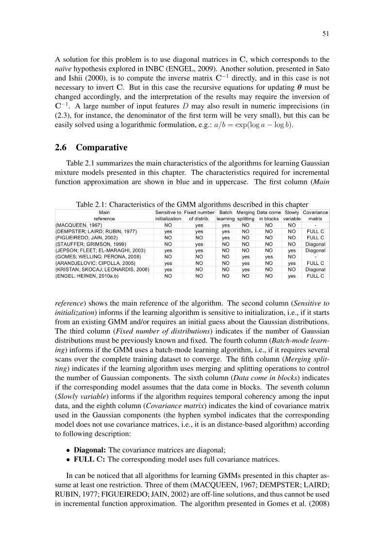
51
A solution for this problem is to use diagonal matrices in C, which corresponds to thenaïve hypothesis explored in INBC (ENGEL, 2009). Another solution, presented in Satoand Ishii (2000), is to compute the inverse matrix C−1 directly, and in this case is notnecessary to invert C. But in this case the recursive equations for updating θ must bechanged accordingly, and the interpretation of the results may require the inversion ofC−1. A large number of input features D may also result in numeric imprecisions (in(2.3), for instance, the denominator of the first term will be very small), but this can beeasily solved using a logarithmic formulation, e.g.: a/b = exp(log a− log b).
2.6 Comparative
Table 2.1 summarizes the main characteristics of the algorithms for learning Gaussianmixture models presented in this chapter. The characteristics required for incrementalfunction approximation are shown in blue and in uppercase. The first column (Main
Table 2.1: Characteristics of the GMM algorithms described in this chapter
reference) shows the main reference of the algorithm. The second column (Sensitive toinitialization) informs if the learning algorithm is sensitive to initialization, i.e., if it startsfrom an existing GMM and/or requires an initial guess about the Gaussian distributions.The third column (Fixed number of distributions) indicates if the number of Gaussiandistributions must be previously known and fixed. The fourth column (Batch-mode learn-ing) informs if the GMM uses a batch-mode learning algorithm, i.e., if it requires severalscans over the complete training dataset to converge. The fifth column (Merging split-ting) indicates if the learning algorithm uses merging and splitting operations to controlthe number of Gaussian components. The sixth column (Data come in blocks) indicatesif the corresponding model assumes that the data come in blocks. The seventh column(Slowly variable) informs if the algorithm requires temporal coherency among the inputdata, and the eighth column (Covariance matrix) indicates the kind of covariance matrixused in the Gaussian components (the hyphen symbol indicates that the correspondingmodel does not use covariance matrices, i.e., it is an distance-based algorithm) accordingto following description:
• Diagonal: The covariance matrices are diagonal;• FULL C: The corresponding model uses full covariance matrices.
In can be noticed that all algorithms for learning GMMs presented in this chapter as-sume at least one restriction. Three of them (MACQUEEN, 1967; DEMPSTER; LAIRD;RUBIN, 1977; FIGUEIREDO; JAIN, 2002) are off-line solutions, and thus cannot be usedin incremental function approximation. The algorithm presented in Gomes et al. (2008)

52
assumes that the training data come in blocks, which is a strong constraint for manyapplications. Other algorithms (STAUFFER; GRIMSON, 1999; JEPSON; FLEET; EL-MARAGHI, 2003) assume that the number of Gaussian distributions is previously knownand fixed, which prevent them to adapt for environment changes and/or learning new con-cepts. The GMM learning algorithms proposed in Jepson et al. (2003), Arandjelovic andCipolla (2005) and Kristan et al. (2008) are sensitive to initialization and/or starts fromexisting GMMs, i.e., they do not tackle the problem of how to initialize the Gaussiandistributions. Moreover, the algorithms presented in Arandjelovic and Cipolla (2005),Gomes et al. (2008) and Kristan et al. (2008) use batch-mode operations (e.g., mergingand splitting) to change the number of distributions.
The GMM learning algorithm proposed in this thesis (last row at Table 2.1), on theother hand, starts from scratch, learns incrementally from data flows, does not assumethat the data come in blocks, is able to create new components on demand and does notuse merging and splitting operations. In fact, the only constraint assumed by IGMM isthat the environment must be locally stable, but this restriction is less severe than thatassumed in Arandjelovic and Cipolla (2005), for instance, because IGMM can deal evenwith abrupt changes in the input data.

53
3 ARTIFICIAL NEURAL NETWORKS
This chapter presents some state-of-the-art artificial neural network (ANN) modelsrelated to this thesis, their main characteristics and limitations. Initially Section 3.1describes the Multi-layer Perceptrons (MLP) (RUMELHART; HINTON; WILLIAMS,1986) architecture, which is the most well known and used neural network model. ThenSection 3.2 presents the radial basis functions (RBF) network (POWELL, 1985, 1987a,b),which is an important kind of neural network used mainly in non-linear regression. Sec-tion 3.3 describes the self-organizing map (SOM) (KOHONEN, 1990, 2001), an unsu-pervised ANN model characterized by the formation of a topological map from the inputpatterns. Sections 3.4 and 3.5 describe, respectively, the ART (CARPENTER; GROSS-BERG, 1987) and ARTMAP (CARPENTER; GROSSBERG; REYNOLDS, 1991) mod-els, which are ANNs based on the adaptive resonance theory (GROSSBERG, 1976a,b,2000). Sections 3.6 and 3.7 present, respectively, the PNN (SPECHT, 1988, 1990) andGRNN (SPECHT, 1991) networks, which are probabilistic models that learn instanta-neously using a single presentation of each training sample. Section 3.8 shows someimprovements made over PNN and GRNN to tackle their main limitations, specially therequirement of a separate neuron for each training pattern. Section 3.9 describes other notwell known but interesting ANN models. Finally, Section 3.10 summarizes and comparesthe neural network models described in this chapter.
3.1 Multi-layer Perceptrons
Multi-layer Perceptrons (MLP) (RUMELHART; HINTON; WILLIAMS, 1986) rep-resent the most prominent and well researched class of ANNs for classification and func-tion approximation, implementing a feed-forward and supervised learning paradigm. Itconsists of several layers of neurons, interconnected through weighted acyclic arcs fromeach preceding layer to the following, without lateral or feedback connections. Each nodecomputes a transformed weighted combination of its inputs of the form
yj(n) = ϕ(vj(n)) (3.1)
where ϕ(·) is the activation function and vj(n) is the induced local field of the neuron j,defined by
vj(n) =D∑i=0
wji(n)yi(n) (3.2)
where D is the total number of inputs applied to neuron j, and wji is the synaptic weightconnecting neuron i to neuron j, and yi(n) is the input signal of neuron j or equivalently,

54
the function signal appearing at the output of neuron i. A commonly used activationfunction is the logistic function given by:
yj(n) =1
1 + exp(−vj(n)). (3.3)
The algorithm used to train MLP networks, called Backpropagation (RUMELHART;HINTON; WILLIAMS, 1986), is a supervised learning method based on gradient descentwhich generalizes the Delta rule proposed by Widrow and Hoff (1960).
MLPs are useful in function approximation because they can approximate any givencontinuous function on any compact subset to any degree of accuracy, provided that asufficient number of hidden layer neurons is used (POGGIO; GIROSI, 1989). This isproved by the universal approximation theorem, which asserts that the standard multilayerfeed-forward networks with a single hidden layer that contains finite number of hiddenneurons, and with arbitrary activation function1 are universal approximators in C(RD)(CSÁJI, 2001). According to Hornik (1991), it is the multilayer feed-forward architectureitself which gives artificial neural networks the potential of being universal approximators,and this potential does not depend on a specific choice of the activation function. It isimportant to say that although the MLP architecture can represent any continuous functiongiven a sufficient number of hidden neurons, this function cannot necessarily be learnedby the Backpropagation algorithm, i.e., the convergence in Backpropagation learning isnot guaranteed (HAYKIN, 2008).
MLPs can be used in classification and regression, but generally not in clusteringtasks. The main disadvantages of MLP are: (i) the Backpropagation algorithm requiresseveral scans (called epochs) over all training data to converge for a good solution, i.e.,to reduce to an acceptable value the error between the desired and actual outputs; (ii)it suffers from the so called “catastrophic interference” (FRENCH, 2003), which occurswhen the newly learned patterns suddenly and completely erase the network memory ofthe previously learned patterns; (iii) the neural network topology (i.e., number of hiddenlayers and the number of neurons in each hidden layer) must be defined a priori andkept fixed; (iv) the learning algorithm has many critical parameters (e.g., learning rate,momentum, weight decay) which must be finely tuned for the learning process to properlyoccur. The neural network topology and the configuration parameters are usually set ina trial and error process, which requires several hours of a human specialist, and theobtained configuration is specific for the current task (there is no default values that workin most cases). Some of these problems are tackled by incremental ANN models, like theFahlman’s Cascade Correlation (FAHLMAN; LEBIERE, 1990), which automatically setsthe neural architecture and the learning parameters. But these models still require severalscans over the entire training dataset to converge.
3.2 Radial basis function networks
Radial basis functions (RBF) networks (POWELL, 1985, 1987a,b) constitute a widelyused and researched tool for nonlinear function approximation. They typically have threelayers: an input layer, a hidden layer with a non-linear RBF activation function and a
1ϕ is an activation function if and only if ϕ is bounded and limx→+∞
ϕ(x) = a, limx→−∞
ϕ(x) = b, a 6= b.

55
linear output layer. The output, ϕ : RD → R, of the network is thus
ϕ(x) =M∑i=1
wiρ(‖x− µi‖) (3.4)
where M is the number of neurons in the hidden layer, µi is the center vector of theneuron i, and wi are the weights of the linear output neuron. In its basic form all inputsare connected to each hidden neuron. The norm is typically the Euclidean distance andthe basis functions are generally Gaussian, i.e.,
ρ(‖x− µi‖
)= exp
[−β ‖x− µi‖2
]. (3.5)
The Gaussian basis functions are local in the sense that changing parameters of one neuronhas only a small effect for input values that are far away from the center of that neuron,i.e.:
lim‖x‖→±∞
ρ(‖x− µi‖) = 0 (3.6)
This local effect is specially useful in tasks like reinforcement learning (SUTTON; BARTO,1998), because it prevents that the knowledge acquired in a region not recently visited bedestroyed by changes made in other regions of the state space (SMART, 2002).
RBF networks are universal approximators on a compact subset of RD (POWELL,1987a; SHAHSAVAND, 2009). This means that a RBF network with enough hidden neu-rons can approximate any continuous function with arbitrary precision. The parameterswi, µi, and β are determined in a manner that optimizes the fit between ϕ and the data. Ingeneral RBF networks are used just in regression tasks.
3.3 Self-organizing maps
A self-organizing map (SOM), also called a Kohonen map (KOHONEN, 1990, 2001),is an artificial neural network model that is trained using unsupervised learning to producea low-dimensional, discretized representation of the input space. In a self-organizingmap, the neurons are placed at the nodes of a lattice, that is usually one-dimensionalor two-dimensional. Through a competitive learning process, the neurons of the latticebecome ordered with respect to each other in such a way that a meaningful coordinatesystem for input features is created over the lattice (KOHONEN, 2001). SOM is thereforecharacterized by the formation of a topographic map of the input patterns, in which thespatial locations of the neurons indicate intrinsic statistical features of the input patterns(HAYKIN, 2008).
The competitive learning process used by SOM works as follows. Initially the weightvectors wjMj=1 are chosen either to small random values or sampled evenly from theavailable set of input training vectors xiNi=1. Using the latter alternative the learningprocess is usually faster because the initial weights are already good approximations ofthe SOM weight vectors (KOHONEN, 2001). When a training sample xt is fed to thenetwork, the neuron with weight vector most similar to the input vector, i.e., the winningneuron i(x), is computed through
i(x) = arg minj‖xt −wj‖, j = 1, 2, . . . ,M . (3.7)
After this, the synaptic weight vectors of all neurons are adjusted using the followingupdate equation:
w∗j = wj + ηthj,i(x)(xt −wj), (3.8)

56
where ηt is the learning rate parameter and hj,i(x) is the neighborhood function centeredaround the winning neuron i(x). A common choice for the neighborhood function is theGaussian function:
hj,i(x) = exp
(−d2j,i2σ2
), (3.9)
where σ is a parameter that controls the size of the topology and dj,i is the Euclideandistance between the lattice positions of neuron j, rj , and the winning neuron i(x), ri:
dj,i = ‖rj − ri‖. (3.10)
A requirement of the SOM learning algorithm is that the size of the topological neighbor-hood shrinks with time, which is achieved using an exponential decay of σ:
σt = σ0 exp
(− t
τ1
), t = 0, 1, 2, . . . (3.11)
where σ0 is the initial value of σ and τ1 is a time constant set by the user. Anotherrequirement of the learning algorithm is that the learning rate ηt must decrease graduallywith increasing time t, which is also achieved using an exponential decay:
ηt = η0 exp
(− t
τ2
), t = 0, 1, 2, . . . (3.12)
where η0 is the initial value of η and τ2 is another time constant set by the user. Thelearning process is repeated for each input vector x for a (usually large) number of epochsuntil no noticeable changes in the feature map are observed (KOHONEN, 2001).
SOM is very useful for clustering and visualizing high-dimensional data, because itdescribes a mapping from a higher dimensional input space to a lower dimensional, typi-cally two-dimensional, map space. Its main limitations are: (i) the learning algorithm re-quires several epochs to converge; (ii) there are separate phases for training and mapping,i.e., the standard SOM cannot learn continuously; and (iii) the neural network architecture(number of neurons in the lattice) must be previously configured and kept fixed. Some ofthese drawbacks are tackled by variations of the SOM architecture, like GTSOM (BAS-TOS, 2007; MENEGAZ; ENGEL, 2009), which can automatically set the neural networkarchitecture during learning in an incremental way. Moreover, GTSOM has no separatephases for training and mapping, i.e., it can learn continuously and perpetually. However,GTSOM still requires many training epochs to converge.
3.4 Adaptive Resonance Theory
Adaptive resonance theory (ART) is a theory developed by Grossberg (1976a; 1976b)on aspects of how the brain processes information (GROSSBERG, 1982). It describes anumber of neural network models (e.g., ART1, Fuzzy ART, ARTMAP), that uses super-vised and unsupervised learning methods, and addresses problems such as pattern recog-nition and prediction (GROSSBERG, 2000). A central feature of ART is a pattern match-ing process, that compares an external input I with the internal memory of an active code.This matching process leads either to a resonant state, which persists long enough to al-low learning, or to a parallel memory search. If the search ends at an established code, thememory representation may either remain the same or incorporate new information from

57
matched portions of the current input I. If the search ends at a new code, the memoryrepresentation learns the current input I (CARPENTER; GROSSBERG, 2003).
The simplest ART model is an unsupervised learning network called ART1, which ac-cepts only binary input data. Figure 3.1, reproduced from Carpenter and Grossberg (1987),shows its typical architecture, that consists of:
• Two layers of binary neurons: the comparison layer, called F1, and the recogni-tion layer, called F2;• A vigilance parameter, ρ, which specifies the minimum fraction of the input that
must remain in the matched pattern for resonance to occur;• A reset module, that compares the strength of the recognition match to the vigi-
lance parameter ρ.
Figure 3.1: Typical architecture of ART1
The vigilance parameter ρ has considerable influence on the system: higher vigilanceproduces highly detailed memories (many, fine-grained categories), while lower vigilanceresults in more general memories (fewer, more-general categories). By varying ρ the sys-tem can recognize both abstract categories, such as faces and cats, and individual exam-ples of these categories such as my cat (CARPENTER; GROSSBERG, 2003).
There are two sets of synaptic weights connecting F1 and F2 in the ART1 model:
• Bottom-up weights: connecting F1 → F2;• Top-down weights: connecting F2 → F1.
In the following the basic operation of the ART1 learning algorithm is described. Tosimplify our notation, in this section the subscripts i and j will be used exclusively to referto the layers F1 and F2, respectively. Therefore, the neurons on the F1 and F2 layers willbe called, respectively, vi and vj , the top-down (F2 → F1) weights will be called wji and

58
the bottom-up (F1 → F2) weights wij . This notation follows that presented in Freemanand Skapura (1991).
Before the learning process starts, it is necessary to initialize the weights and theneural activities of F1 and F2. The weights of the top-down connections (vj → vi), wji,are initialized according to
wji(0) >B1 − 1
D1
, (3.13)
where B1 and D1 are configuration parameters chosen according to the following con-straints:
D1 ≥ 0maxD1, 1 < B1 < D1 + 1 .
(3.14)
Other configuration parameters are A1 ≥ 0, C1 ≥ 0 and the vigilance parameter ρ, whichmust be chosen in the interval 0 < ρ ≤ 1. The bottom-up weights, connecting F1 → F2,are initialized according to
0 < wij(0) <L
L− 1 +M, (3.15)
where L > 1 is an ART1 constant and M is the number of units on F1. The activities onF2 are then initialized to zero, and the activities on F1 are initialized in the following way:
x1i(0) =−B1
1 + C1
. (3.16)
When a new binary input vector I ∈ 0, 1 is applied to F1, the activities on F1 arecomputed according to
x1i =Ii
1 + A1(Ii +B1) + C1
, (3.17)
and the output vector for F1, S = s1, . . . , si, . . . , sM, is computed through
si = h(x1i) =
1 if x1i > 00 if x1i ≤ 0 .
(3.18)
This output vector S is propagated to F2, and the activities Tj,∀j ∈M , are computed:
Tj =M∑i=1
siwij . (3.19)
These Tj activities are used to compute the outputs on F2:
uj =
1 Tj = maxkTk, ∀k0 otherwise (3.20)
It is important to notice that only the “winning” node of F2, vj , has a nonzero output. Theoutput from F2 is propagated back to F1, and the net inputs from F2 to the F1 units, Vi,are given by:
Vi =N∑j=1
ujwji , (3.21)
the new activities on F1 are recomputed through
x1i =Ii +D1Vi −B1
1 + A1(Ii +D1Vi) + C1
, (3.22)

59
and the new output vector S is recomputed using (3.18). After this, it is necessary todetermine the degree of match between the input pattern I and the top-down template,i.e.:
|S||I|
=
∑Mi=1 si∑Mi=1 Ii
. (3.23)
If |S|/|I| < ρ, then vj is marked as inactive, the outputs of F2 are set to zero and thealgorithm returns to the first step using the original input pattern I. Otherwise, the learningprocess continues updating the bottom-up weights on vj (the “winning” node) only:
wij =
LL−1+|I| if vi is active0 if vi is inactive,
(3.24)
and the top-down weights coming from vj only to all F1 units are updated through:
wji =
1 if vi is active0 if vi is inactive. (3.25)
Finally, the input pattern is removed, all inactive units on F2 are restored and the algorithmproceeds from the beginning using a new input pattern (FREEMAN; SKAPURA, 1991).
As mentioned above, the basic ART1 architecture deals only with binary input pat-terns. But an improved ART architecture, called Fuzzy ART (CARPENTER; GROSS-BERG; ROSEN, 1991), generalizes ART1 for learning stable recognition categories inresponse to both analog and binary input patterns. This improvement is achieved by in-corporating computations from fuzzy set theory (ZADEH, 1965) into the ART1 neuralnetwork. In Fuzzy ART, the crispy intersection operator (∩) is replaced by the fuzzy MINoperator (∧), and the crispy union operator (∪) is replaced by the fuzzy MAX operator(∨). The fast learning operation, for instance, which in ART1 is given by an intersectionbetween I and w: w∗ = I ∩w, in Fuzzy ART is computed using w∗ = I ∧w, where theMIN operator (∧) of fuzzy set theory replaces the intersection operator (∩) used in ART1.
To prevent category proliferation, Fuzzy ART uses a normalization procedure calledcomplement coding, which actually doubles the number of input components, presentingto the network both the original feature vector and its complement. According to Car-penter et al. (1991), “complement coding leads to a symmetric theory in which the MINoperator (∧) and the MAX operator (∨) of fuzzy set theory play complementary roles”.Moreover, it is generally necessary to normalize the input vectors at a preprocessing stageto prevent category proliferation.
The main advantages of the ART1 and Fuzzy ART are (CARPENTER; GROSS-BERG, 2003): (i) they can learn incrementally and continuously, what make them wellsuited for on-line learning of large and evolving databases; (ii) the adaptive resonancetheory tackles the stability-plasticity dilemma and does not suffer from catastrophic inter-ference; (iii) the learning process can be fast, thus enabling a system to adapt quickly toinputs that rarely occur but that may require immediate accurate recall. The main draw-backs of these unsupervised ART models are (SARLE, 1995): (i) they depend criticallyupon the order in which the training data are processed; and (ii) the estimates producedby them do not possess the statistical property of consistency.
3.5 ARTMAP
The ARTMAP model, also called predictive ART (CARPENTER; GROSSBERG;REYNOLDS, 1991), is a neural network classifier that combines two ART modules into

60
a supervised learning structure, where the first module (ARTa) takes the input data aand the second module (ARTb) takes the correct output data b. ARTMAP uses thesemodules to make the minimum possible adjustment of the vigilance parameter of the firstmodule (ρa) in order to make the correct classification or prediction. The main elementsof the ARTMAP architecture are shown in Figure 3.2 (reproduced from Carpenter etal. (CARPENTER; GROSSBERG; REYNOLDS, 1991)).
Figure 3.2: ARTMAP architecture
ARTa and ARTb modules are connected by an inter-ART module, which is in manyaspects similar to an ART1 network (e.g., it receives only binary data). This inter-ARTmodule includes a so called map field F ab, that controls the learning of an associativemap from ARTa to ARTb recognition categories. The map field also controls the matchtracking of the ARTa vigilance parameter ρa. A mismatch at the map field between theARTa category activated by a and the ARTb category activated by b increases ρa by theminimum amount needed for the system to search for and, if necessary, learn a new ARTa
category whose prediction matches the ARTb category (CARPENTER; GROSSBERG;REYNOLDS, 1991).
The match tracking process of ARTMAP works as follows. Assume that x is theoutput vector of the map field F ab, ρ is the vigilance parameter of F ab, yb is the outputvector of F b
2 (the second layer of ARTb), xa is the output vector of F a1 (the first layer of
ARTa), zaj is the top-down input of F b1 and wj is a weight vector that links the jth node
of F a2 to the nodes in F ab. When a new data sample a,b is presented to ARTMAP, the
vigilance parameter of the ARTa module, ρa, is set to be equal a baseline vigilance ρa. If|x| < ρ|yb|, then ρa is increased until it is slightly larger than |a ∩ zaj ||a|−1. Then
|xa| = |a ∩ zaj | < ρa|a|, (3.26)
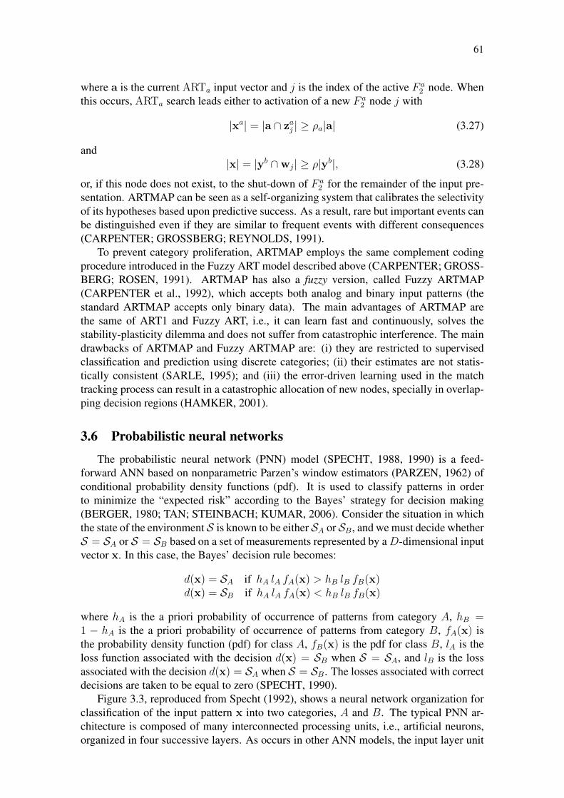
61
where a is the current ARTa input vector and j is the index of the active F a2 node. When
this occurs, ARTa search leads either to activation of a new F a2 node j with
|xa| = |a ∩ zaj | ≥ ρa|a| (3.27)
and|x| = |yb ∩wj| ≥ ρ|yb|, (3.28)
or, if this node does not exist, to the shut-down of F a2 for the remainder of the input pre-
sentation. ARTMAP can be seen as a self-organizing system that calibrates the selectivityof its hypotheses based upon predictive success. As a result, rare but important events canbe distinguished even if they are similar to frequent events with different consequences(CARPENTER; GROSSBERG; REYNOLDS, 1991).
To prevent category proliferation, ARTMAP employs the same complement codingprocedure introduced in the Fuzzy ART model described above (CARPENTER; GROSS-BERG; ROSEN, 1991). ARTMAP has also a fuzzy version, called Fuzzy ARTMAP(CARPENTER et al., 1992), which accepts both analog and binary input patterns (thestandard ARTMAP accepts only binary data). The main advantages of ARTMAP arethe same of ART1 and Fuzzy ART, i.e., it can learn fast and continuously, solves thestability-plasticity dilemma and does not suffer from catastrophic interference. The maindrawbacks of ARTMAP and Fuzzy ARTMAP are: (i) they are restricted to supervisedclassification and prediction using discrete categories; (ii) their estimates are not statis-tically consistent (SARLE, 1995); and (iii) the error-driven learning used in the matchtracking process can result in a catastrophic allocation of new nodes, specially in overlap-ping decision regions (HAMKER, 2001).
3.6 Probabilistic neural networks
The probabilistic neural network (PNN) model (SPECHT, 1988, 1990) is a feed-forward ANN based on nonparametric Parzen’s window estimators (PARZEN, 1962) ofconditional probability density functions (pdf). It is used to classify patterns in orderto minimize the “expected risk” according to the Bayes’ strategy for decision making(BERGER, 1980; TAN; STEINBACH; KUMAR, 2006). Consider the situation in whichthe state of the environment S is known to be either SA or SB, and we must decide whetherS = SA or S = SB based on a set of measurements represented by aD-dimensional inputvector x. In this case, the Bayes’ decision rule becomes:
d(x) = SA if hA lA fA(x) > hB lB fB(x)d(x) = SB if hA lA fA(x) < hB lB fB(x)
where hA is the a priori probability of occurrence of patterns from category A, hB =1 − hA is the a priori probability of occurrence of patterns from category B, fA(x) isthe probability density function (pdf) for class A, fB(x) is the pdf for class B, lA is theloss function associated with the decision d(x) = SB when S = SA, and lB is the lossassociated with the decision d(x) = SA when S = SB. The losses associated with correctdecisions are taken to be equal to zero (SPECHT, 1990).
Figure 3.3, reproduced from Specht (1992), shows a neural network organization forclassification of the input pattern x into two categories, A and B. The typical PNN ar-chitecture is composed of many interconnected processing units, i.e., artificial neurons,organized in four successive layers. As occurs in other ANN models, the input layer unit
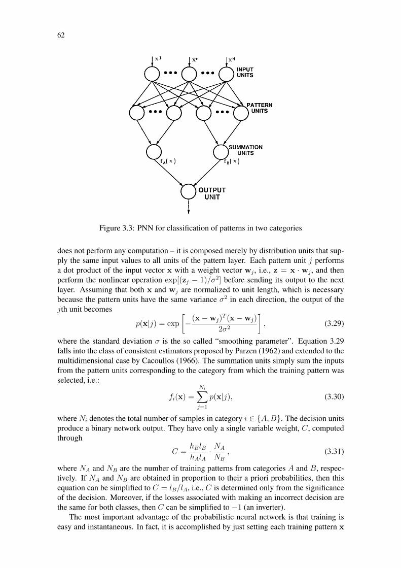
62
Figure 3.3: PNN for classification of patterns in two categories
does not perform any computation – it is composed merely by distribution units that sup-ply the same input values to all units of the pattern layer. Each pattern unit j performsa dot product of the input vector x with a weight vector wj , i.e., z = x · wj , and thenperform the nonlinear operation exp[(zj − 1)/σ2] before sending its output to the nextlayer. Assuming that both x and wj are normalized to unit length, which is necessarybecause the pattern units have the same variance σ2 in each direction, the output of thejth unit becomes
p(x|j) = exp
[−(x−wj)
T (x−wj)
2σ2
], (3.29)
where the standard deviation σ is the so called “smoothing parameter”. Equation 3.29falls into the class of consistent estimators proposed by Parzen (1962) and extended to themultidimensional case by Cacoullos (1966). The summation units simply sum the inputsfrom the pattern units corresponding to the category from which the training pattern wasselected, i.e.:
fi(x) =
Ni∑j=1
p(x|j), (3.30)
where Ni denotes the total number of samples in category i ∈ A,B. The decision unitsproduce a binary network output. They have only a single variable weight, C, computedthrough
C =hBlBhAlA
· NA
NB
, (3.31)
where NA and NB are the number of training patterns from categories A and B, respec-tively. If NA and NB are obtained in proportion to their a priori probabilities, then thisequation can be simplified to C = lB/lA, i.e., C is determined only from the significanceof the decision. Moreover, if the losses associated with making an incorrect decision arethe same for both classes, then C can be simplified to −1 (an inverter).
The most important advantage of the probabilistic neural network is that training iseasy and instantaneous. In fact, it is accomplished by just setting each training pattern x

63
equal to the wj weight vector in one of the pattern units, and then connecting the outputof the pattern unit to the appropriate summation unit. Another advantage of PNN is thatit is guaranteed to asymptotically approach the Bayes’ optimal decision surface providedthat the class pdfs are smooth and continuous (RUTKOWSKI, 2004a).
The main drawback of PNN is that a separate neuron (pattern unit) is required forevery training pattern, so in large databases an enormous amount of storage memory maybe required (BHATTACHARYYA et al., 2008). Moreover, the amount of computationnecessary to classify an unknown pattern x is proportional to the size of the training set.Another limitation of PNN is that all pattern units are “isotropic Gaussians”, i.e., theyhave the same width σ in each dimension, which makes PNN not robust with respect toaffine transformations of feature space (MONTANA, 1992). Moreover, the smoothingparameter σ is critical and must be properly configured to obtain good results. Spechtsuggests to use the holdout method (FUKUNAGA, 1990; TAN; STEINBACH; KUMAR,2006) for setting the σ parameter, but this method requires repeating the training processN times using the entire dataset.
3.7 General regression neural network
The general regression neural network (GRNN), proposed by Specht (1991), falls intothe category of probabilistic neural networks described above. It is a memory-based net-work based on the theory of nonlinear kernel regression (BISHOP, 1995), which providesestimates of continuous variables and converges to the underlying regression surface. Themathematical formulation of GRNN is given as follows. Assume that f(X, Y ) representsthe known joint continuous pdf of a vector random variable, X, and a scalar random vari-able, Y . Let x be a particular measured value of X. The conditional mean of Y given x,also called the regression of Y on x, is given by
E[Y |x] =
∫ ∞−∞
Y f(x, Y )dY∫ ∞−∞
f(x, Y )dY
. (3.32)
When the density f(X, Y ) is not known, it must be usually estimated from the obser-vations x and y. GRNN uses the class of consistent estimators proposed by Parzen (1962)and extended to the multidimensional case by Cacoullos (1966) for a nonparametric esti-mate of f(X, Y ). Using these nonparametric estimators, the conditional mean y becomes:
y =
N∑i=1
yi exp
(−(x− xi)T (x− xi)
2σ2
)N∑i=1
exp
(−(x− xi)T (x− xi)
2σ2
) , (3.33)
where N is the number of sample observations and xi is the ith observation of the vectorrandom variable X.
The architecture of a typical GRNN consists of four successive layers of processingunits, as shows Figure 3.4 reproduced from Specht (1991). The input layer is composedmerely by distribution units, but it is usually necessary to scale all input variables suchthat they have approximately the same ranges or variances. This is necessary because
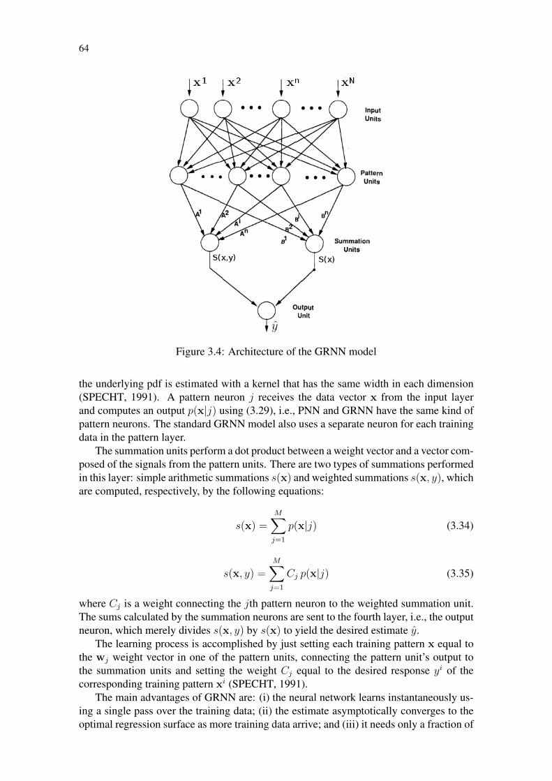
64
Figure 3.4: Architecture of the GRNN model
the underlying pdf is estimated with a kernel that has the same width in each dimension(SPECHT, 1991). A pattern neuron j receives the data vector x from the input layerand computes an output p(x|j) using (3.29), i.e., PNN and GRNN have the same kind ofpattern neurons. The standard GRNN model also uses a separate neuron for each trainingdata in the pattern layer.
The summation units perform a dot product between a weight vector and a vector com-posed of the signals from the pattern units. There are two types of summations performedin this layer: simple arithmetic summations s(x) and weighted summations s(x, y), whichare computed, respectively, by the following equations:
s(x) =M∑j=1
p(x|j) (3.34)
s(x, y) =M∑j=1
Cj p(x|j) (3.35)
where Cj is a weight connecting the jth pattern neuron to the weighted summation unit.The sums calculated by the summation neurons are sent to the fourth layer, i.e., the outputneuron, which merely divides s(x, y) by s(x) to yield the desired estimate y.
The learning process is accomplished by just setting each training pattern x equal tothe wj weight vector in one of the pattern units, connecting the pattern unit’s output tothe summation units and setting the weight Cj equal to the desired response yi of thecorresponding training pattern xi (SPECHT, 1991).
The main advantages of GRNN are: (i) the neural network learns instantaneously us-ing a single pass over the training data; (ii) the estimate asymptotically converges to theoptimal regression surface as more training data arrive; and (iii) it needs only a fraction of

65
the training samples a MLP neural network would need to converge. The main disadvan-tage of the standard GRNN is the amount of computation required to evaluate new points,which is proportional to the size of the training dataset.
To overcome this problem, Specht (1991) suggest to use clustering algorithms, likeK-means averaging (TOU; GONZALEZ, 1974) or adaptiveK-means (MOODY; DARKEN,1989), to group samples so that the group can be represented by a single pattern unit.In this case, each weight vector wj represents the center of a cluster and (3.33) can berewritten as
y =
M∑j=1
Aj exp
(−(x−wj)
T (x−wj)
2σ2
)M∑j=1
Bj exp
(−(x−wj)
T (x−wj)
2σ2
) , (3.36)
where M < N is the number of clusters, Aj is the sum of the y values and Bj is thenumber of samples assigned to cluster j. Aj and Bj are incremented each time a trainingobservation yi for the jth cluster is encountered, i.e.:
Aj∗ = Aj + yi
Bj∗ = Bj + 1 .(3.37)
In Specht (1991) other cluster techniques to set the pattern units are suggested, butthose techniques: (i) are restricted to distance-based algorithms (e.g., theK-means and itsvariations); (ii) require that the number of clusters be previously known and fixed; and/or(iii) are based in ad-hoc choices like the definition of a radius of influence r. Anotherproblem of the GRNN model is the configuration of the smoothing parameter σ, which asin PNN must be done off-line using iterative techniques like the holdout method (TAN;STEINBACH; KUMAR, 2006).
3.8 Improvements made over PNN and GRNN
As mentioned above, the standard PNN and GRNN architectures have several limita-tions which makes the computation very slow for large databases and/or prevents their usein on-line and continuous tasks. This section describes some state-of-the-art approachesto tackle these limitations. Most part of these approaches use some kind of clusteringalgorithm to group the input patterns, so that the group can be represented by a single unitin the pattern layer.
In Tråvén (1991), a Gaussian clustering (GC) algorithm is proposed for substantiallyreducing the amount of information necessary to consider during classification. This al-gorithm uses radially symmetric Gaussian components whose parameters are estimatedby a stochastic gradient descent procedure (WOLFE, 1970). In this procedure, the meanof each Gaussian distribution (i.e., cluster) j is updated through:
µ∗j = µj + ηj(xt − µj), (3.38)
where xt is the current input pattern and ηj is given by:
ηj =p(j|xt)Np(j)
, (3.39)

66
where p(j|xt) is the posterior probability of j given xt, N is the number of trainingpatterns received until the current time t (i.e., N ≡ t) and p(j) is the a priori probabilityof j. GC assumes that the prior probabilities of all clusters are the same, i.e., p(j) = 1/M ,where M is the number of Gaussian distributions. It also assumes that the covariancematrices are in the form of a constant times the identity matrix, i.e., C = σ2I. The updateequation for the variance σ2 is:
σ2∗j = σ2
j + ηj
[2
D(1− xt · µTj )− σ2
N
], (3.40)
where the superscript ‘T ’ denotes the transpose and D is the dimensionality of x. Apeculiarity of this algorithm is that the parameters of the pattern units depend only on theinput densities, which according to Tråvén (1991) “in some cases may result in somewhatless efficient solutions compared with methods where the placement of the hidden unitscan be supervised”. The main limitations of this algorithm are: (i) it uses only radiallysymmetric pdf’s; (ii) it assumes that all prior probabilities are equal; (iii) the number ofclusters must be previously defined and fixed; and (iv) there are separate phases fromtraining and recalling, that prevents its use in on-line and continuous tasks.
In Cwik and Koronacki (1996), the Tråvén’s GC algorithm is extended so that noconstraints are imposed on the covariance matrices, i.e., the updated covariance matrixC∗j of the jth Gaussian distribution is computed through:
C∗j = Cj + ηj[(xt − µj)(x
t − µj)T −Cj
]. (3.41)
where ηj is computed using (3.39) above. Unfortunately this algorithm still requires thatthe number of clusters must be previously known and fixed. Moreover, The Gaussiancomponents are initialized using the off-line K-means algorithm (MACQUEEN, 1967).
In Montana (1992) a genetic algorithm (GOLDBERG, 1989; MITCHELL, 1996) isused to optimize the covariance matrices of the pattern units, thus allowing anisotropicGaussians units, i.e. Gaussians whose covariance is not a multiple of the identity ma-trix, in the pattern layer. This optimization method, called weighted probabilistic neuralnetwork (WPNN), works as follows. For ith exemplar of class j, xji , let Lj(xji ), forj = 1, . . . ,M , denote the class likelihoods obtained upon withholding this exemplar andapplyingN (x|µj,Cj), and let Pj(x
ji ) be the probabilities obtained from these likelihoods
through:
Pj(xji ) = Lj(xji )/
M∑q=1
Lq(xqi ) (3.42)
Then, the fitness of the GA is defined as
E =M∑j=1
Nj∑i=1
((1− Pj(xji ))2 +∑q 6=j
(Pq(xji ))
2) . (3.43)
where Nj is the number of training samples of class j. In Mao et al. (2000) another GA-based algorithm to determine the structure of a PNN network is proposed. This algorithmconsists of two parts and runs in an iterative way. The first part identifies an appropriatesmoothing parameter using a genetic algorithm, while the second part determines suitablepattern layer neurons using a forward regression orthogonal algorithm (CHEN; COWAN;GRANT, 1991). The main disadvantage of these GA-based methods is that they requirea large number of generations to evolve a good solution.

67
In Streit and Luginbuhl (1994), a maximum likelihood method for training probabilis-tic networks is proposed. This training method, called Generalized Fisher (GF) training,is an iterative procedure that computes stationary points of the posterior likelihood func-tion L without taking gradients or derivatives. It begins with an initial guess, θ, for theoptimum parameters, and each iteration gives a new parameter estimate, θ+, that is guar-anteed to increase the value of the posterior likelihood function L unless θ is a stationaryvalue of L. By restarting the GF training algorithm with different initial guesses θ, andchoosing the best of the local maxima so obtained, a satisfactory maximum likelihoodestimate for θ can be found. GF is based on the premise that all classes are multivari-ate Gaussian random variables with a common covariance matrix C, but different meanvectors µj . Initially the labeled training set X is partitioned into the disjoint subsetsX = X1 ∪ T2 ∪ · · · ∪ XM , where M is the number of classes and Xj comprises thosesamples in X with class label j. The sample means of the jth class are estimated through
µj =1
Nj
Nj∑i=1
xi (3.44)
where xi is the ith training pattern of class j and Nj is the number of training samples inj. The common covariance matrix C is estimated by Fisher’s within-class scatter matrix:
C =1
N
M∑j=1
Nj∑i=1
(xi − µj)(xi − µj)
T . (3.45)
where N denotes the total number of samples of the training dataset. The estimation errorfor C is reduced by pooling the sample data, i.e., by using all samples in the training set X.The a priori probabilities are computed without iteration using p(j) = Nj/N . The mainlimitations of this method are: (i) all pattern units share the same covariance matrix, whichworks well only when “samples from different classes have broadly similar correlationalstructure” (STREIT; LUGINBUHL, 1994); (ii) it is an iterative procedure whose resultsdepend strongly on the initial guess θ; (iii) the number of Gaussian units must be specifiedbefore the actual training can take place; and (iv) it is somewhat restricted to classification,because the training dataset must be partitioned into the disjoint subsets.
In Berthold and Diamond (1998), a learning algorithm that constructs the topologyof a probabilistic neural network during training is proposed. This algorithm, called dy-namic decay adjustment (DDA), has two configuration parameters, the thresholds θ+ andθ−. θ+ determines the minimum correct-classification probability for training patterns ofthe correct class, and θ− is used to avoid misclassifications. The operation requires twodistinct phases: training and classification. The training phase works as follows. Initiallyall prototype weights A are set to zero, i.e., Aki = 0, ∀pki , where pki is the ith prototype(candidate) neuron of the output class k. Next all training patterns are presented to theneural network. If a pattern (x, k) is classified correctly, i.e., ∃pki : N (x,µki , σ
ki ) ≥ θ+),
the weight of the prototype with the largest variance, Aki , is increased (Aki = Aki + 1.0).Otherwise a new prototype is introduced (Mk = Mk + 1) having the new pattern as itscenter (µk
Mk = x), a prototype weight AkMk equal to 1 (Ak
Mk = 1), and its initial radiusσkMk is set as large as possible without misclassifying an already existing prototype of
conflicting class, i.e.:
σkMk = minl 6=k
1≤j≤M l
√−‖µlj − µk
Mk‖2
ln θ−
. (3.46)

68
After this all the prototypes 1 ≤ j ≤ M l of the conflicting classes l 6= k are shrunk iftheir activations are too high for this specific pattern, i.e.:
σlj = min
σlj,√−‖x− µlj‖2
ln θ−
,∀j ∈Mk. (3.47)
The learning process is repeated for some epochs until the network architecture settles,thus indicating the completion of the training phase. After training is complete, the nor-malized output weights wkj are computed for each class k from the prototype weights Akjthrough:
wkj =Akj∑Mk
q=1Akq
, ∀j ∈Mk . (3.48)
The main limitations of this algorithm are: (i) it is a batch-mode algorithm which requiresthat the entire training dataset must be previously known and fixed; (ii) there are distinctphases for training and classification; (iii) it uses just radially symmetric Gaussian kernels;and (iv) the center µ of a pattern unit never changes after its introduction, i.e., just thestandard deviation σ of each distribution is adjusted during learning.
Delgosha and Menhaj (2001) propose a modified PNN learning algorithm, calledFuzzy PNN (FPNN), which aims to improve the reliability of classification when the out-put classes overlap. This is accomplished by making a soft decision in the training phaseinstead of the traditional hard decision made by traditional classifiers. In the soft decision,the effect of overlapping portions is lessened, because “the classifier is intentionally madeblind with respect to overlapping sections” (DELGOSHA; MENHAJ, 2001). The softdecision is performed by the following smooth penalty function:
ρ(m; b, s) =
0, m < 0
1/(1 + e−(m−b)/s), m ≥ 0(3.49)
where b is a bias introduced for more robustness, s is the softness parameter and m =lj − lq is the difference between the losses of a class j (lj) and the class q 6= j with theminimum risk lq among all classes. The training steps of FPNN are completely similarto those of PNN except the last step: FPNN counts the total number of misclassifiedsample vectors and repeats the training procedure until all the sample vectors are correctlyclassified.
There are other improvements made over probabilistic networks to adapt them tospecific situations. Rutkowski, for instance, derives a new mathematical formulationfor GRNN (RUTKOWSKI, 2004b) and PNN (RUTKOWSKI, 2004a) in time-varyingenvironments, but his formulation has the same drawbacks of the Specht’s models de-scribed above (e.g., a separate neuron is required for every training pattern). Polat andYildirim (2010) describe a hardware implementation of a general regression neural net-work using field programmable gate array (FPGA) circuits. Chang et al. (2009) present aPNN model which has data imputation capabilities for machine-fault classification. Thismodel uses the standard EM algorithm to train the neural network and a global k-meansalgorithm is used prior to EM to find the number of clusters based on minimizing theclustering error.
We can conclude that, although many algorithms have been proposed to tackle themain restrictions of PNN and GRNN, most of them have at least one of the followinglimitations: (i) they are restricted to classification tasks; (ii) they require that the complete

69
training dataset is previously known and fixed; (iii) the learning process requires severalscans over the entire dataset; (iv) they impose limitations on the form of the pattern units;(v) they have separate phases for training and recalling; or (vi) the neural network topol-ogy must be defined a priori and kept fixed. Therefore, these algorithms are not useful forapplications such as incremental function approximation, on-line prediction and mobilerobotics.
3.9 Other neural network models
This section presents other neural network models which are less known and used thanthe traditional models (e.g., MLP, RBF, SOM) described in the previous sections. In Lin etal. (1997), an ANN model called probabilistic decision-based neural network (PDBNN) isproposed. PDBNN has a modular architecture composed by several subnets connected toa decision unit. Learning in PDBNN is divided into two phases: locally unsupervised andglobally supervised. In the locally unsupervised learning phase, PDBNN adopts the EMalgorithm (DEMPSTER; LAIRD; RUBIN, 1977) to maximize the likelihood function
L(X) =N∑t=1
log
[M∑j=1
p(k) p(xt|k,θj)
](3.50)
where k is the output class, X = x1,x2, . . . ,xN denotes the set of N independent andidentically distributed training patterns, θj = µj,Cj, p(k) represents the parameters ofthe jth mixture component,M is the number of mixture components and p(xt|k,θj) is theclass likelihood function computed using a D-variate Gaussian distribution. In the glob-ally supervised training phase, target values are used to fine-tune the decision boundaries.Specifically, when a training pattern is misclassified to the jth class, reinforced and/oranti-reinforced learning (SUTTON; BARTO, 1998) are applied to update the mean vec-tors and covariance matrices of subnet j. The main drawbacks of this algorithm are thesame of great part of the ANN models, i.e.: (i) the learning process requires several scansover the entire dataset; and (ii) there are separate phases for training and recalling.
In Williamson (1997) a probabilistic version of Fuzzy ARTMAP, called GaussianARTMAP, is proposed for mixture modeling and classification. Gaussian ARTMAP dif-fers from Fuzzy ARTMAP significantly in a few respects. First, it represents category j asa Gaussian density function, defined by two vectors: its mean µj = µj1, µj2, . . . , µjMand its standard deviation σj = σj1, σj2, . . . , σjM, which together replace prototypevector wj . Second, a scalar, nj , accumulates the amount of relative activation obtained byF2 node j on training set patterns. During training, the number of committed F2 nodes,Nc, is initially set to 0. Newly-committed F2 nodes increment Nc, and undergo the ini-tialization step:
µJ = A; σJi = γ wabJK = 1; nJ = 1,
where A represents the input pattern, wabJK is the F ab prototype vector connecting nodes Jand K (the inter-ART module still has a prototype vector w) and γ is the initial standarddeviation assigned to newly-committed F2 nodes. Committed F2 nodes that pass thefollowing vigilance test for pattern a:
Gj(A) = exp
−1
2
M∑i=1
(Ai − µji)2
σ2ji
> ρ , (3.51)

70
where ρ are the choice is the baseline vigilance parameter, are allowed to activate, anddistribute a pattern of activity y, i.e.:
yj =gj
0.01 +∑Nc
l=1 gl. (3.52)
Match tracking and learning are performed according to the relative activation over the“ensemble” EK of F2 nodes linked to the predicted F ab node K, i.e.:
ρ′ = exp
−1
2
∑j∈EK
y∗j
M∑i=1
(Ai − µji)2
σ2ji
+ ε . (3.53)
The relative activation over EK is defined by the distributed pattern y∗, where y∗j =yj/∑
l∈EKyl only if j ∈ EK , and y∗j = 0 otherwise. The prototype update is computed
through the following equations:n′j = nj + y∗j (3.54)
µ′ji =
(1−
y∗jnj
)µji +
y∗jnjAi (3.55)
σ′ji =
√(1−
y∗jnj
)σ2ji +
y∗jnj
(Ai − µji)2 . (3.56)
Although the Gaussian ARTMAP can achieve better results than Fuzzy ARTMAP inincremental classification tasks (GRANGER; CONNOLLY; SABOURIN, 2008), it hasmany critical parameters (the “standard” Fuzzy ARTMAP parameters plus ε, ρ, γ), whichmust be properly configured before the learning process starts. Moreover, it uses diagonalcovariance matrices in the Gaussian units, i.e., just the variance σ2 is computed.
Other interesting neural network models are: (i) the recurrent log-linearized Gaus-sian mixture network (R-LLGMN), proposed by Tsuji et al. (2003), which uses Gaussianmixtures and hidden Markov models (HMM) for classifying temporal series. But unfor-tunately this model is not on-line nor incremental, just recurrent; and (ii) the resourceallocating network (RAN), proposed by Platt (1991), which adds new neurons incremen-tally by choosing what training vectors it must store. RAN is based on a distance basedalgorithm, and like K-means the induced model is equivalent to a set of equiprobablespherical distributions sharing the same variance. Moreover, the training algorithm usesthe same (slow) least mean squares (LMS) algorithm (WIDROW; HOFF, 1960) used byBackpropagation (RUMELHART; HINTON; WILLIAMS, 1986).
3.10 Comparison among the described ANN models
Table 3.1 summarizes the main characteristics of the neural network models presentedin this chapter. These characteristics refer to the standard architectures described in thecorresponding papers, but of course some of these models have variations which improvessome of these characteristics and/or extends them for using in other tasks.
The first (neural network) and second (main reference) columns of Table 3.1 present,respectively, the acronyms of the neural network models and the corresponding refer-ences. The third column (main tasks) describes the tasks in which the ANN model ca beused (classification, regression or clustering). The fourth column (incr. arch.) indicatesif the ANN model has an incremental architecture: “YES” means that the neural network

71
Table 3.1: Characteristics of the described neural network models
incrementally adds neurons whenever necessary and “no” means that it uses a predefinedand fixed architecture. The fifth column (cont. learn.) indicates if the neural networkcan learn continuously without separate phases for training and using. The sixth column(inst. learn.) indicates if the model can learn instantaneously with a single presentation ofeach training pattern (“YES”) or it requires several scans over the entire training database(i.e., epochs) to converge (“no”). The seventh column (init. dep.) indicates if the resultsobtained using the corresponding model varies according to the initial conditions, e.g., ifthe random initialization of the model parameters affects significantly the obtained results(which occurs, for instance, when the ANN is sensible to local minima). The eighth col-umn informs if the neural network follows a probabilistic framework or not. In this thesiswe are mainly interested in probabilistic models, because they allow better results in somekind of tasks likes robotics (THRUN; BURGARD; FOX, 2006). The Ninth column (co-var. matrix) indicates the kind of covariance matrix used by each probabilistic model (thehyphen symbol indicates that the corresponding model does not use covariance matrices)according to following description:
• Unique σ: all Gaussian units are radially symmetric and share the same standarddeviation σ;• Radially: each Gaussian unit j has its own standard deviation parameter σj , but
these units are still radially symmetric;• Diagonal: the covariance matrices are diagonal, i.e., the input features are consid-
ered conditionally independent (that corresponds to the naïve Bayes hypothesis);• Unique C: all Gaussian units share the same (full) covariance matrix C;• FULL C: each Gaussian unit j has its own (full) covariance matrix Cj; i.e., no
restrictions are imposed to the shape of the Gaussian distributions.
The tenth column (many units) indicates if the neural network requires a separate neuronfor every training pattern, such as in Specht’s PNN and GRNN. The last column (many

72
conf.) indicates if the ANN has many (critical) configuration parameters which must beproperly configure before learning.
Observing Table 3.1 it can be noticed that neither of these previous approaches satisfyall requirements (written in uppercase in the respective columns) for using them success-fully in incremental function approximation and on-line tasks. The neural network modelproposed in this thesis (last row in Table 3.1), on the other hand, satisfies all these re-quirements, and thus is a suitable tool to be used in this kind of application. Next chapterdescribes the proposed neural network model, called IGMN, in details.

73
4 INCREMENTAL GAUSSIAN MIXTURE NETWORK
This chapter presents the neural network model proposed in this thesis, called IGMN1
(standing for Incremental Gaussian Mixture Network) (HEINEN; ENGEL, 2010a,b), thatis the main contribution of this thesis. It is based on parametric probabilistic models(Gaussian mixture models), that have nice features from the representational point ofview, describing noisy environments in a very parsimonious way, with parameters thatare readily understandable. IGMN can be seen as a supervised learning extension of theIGMM algorithm, presented in Section 2.5, but it has unique features from the statisticalpoint of view that endow it with the ability to make on-line predictions for forward andinverse problems and also to compute the confidence estimates of its predictions, as willbe shown throughout this thesis.
This chapter is structured as follows. Section 4.1 provides the mathematical deriva-tion of the regression algorithm used by IGMN to approximate functions and make pre-dictions. Section 4.2 presents the neural network architecture of IGMN. Section 4.3 de-scribes the operation of IGMN during learning and recalling. Section 4.4 extends theproposed ANN model for multi-valued inverse problems which are not characterized bya functional (i.e. single-valued) mapping. Section 4.5 discusses the IGMN configurationparameters and how they can be set. Finally, Section 4.6 concludes this chapter summa-rizing the main characteristics and limitations of IGMN.
4.1 General regression using Gaussian mixture models
This section describes the statistical basis of IGMN and the mathematical derivation ofthe general regression algorithm which enables IGMN to approximate functions and makepredictions. Suppose that we have a noisy training data set z composed by two data vec-tors, a ∈ A and b ∈ B, that correspond to the observed (i.e., the independent variables)and missing (i.e., the target values) stimuli, respectively. According to Bishop (1995), thegoal of learning is to find a smooth mapping from a to b which captures the underlyingsystematic aspects of the data, without fitting the noise on the data. In Bishop (1995) itis shown that, under many circumstances, the optimal mapping is given by forming theregression, or conditional average 〈b|a〉, of the target data b, conditioned on the inputvariables. This can be expressed in terms of the conditional density p(b|a), and hence interms of the joint density p(a,b), as follows:
b = 〈b|a〉1Initially IGMN was called IPNN (standing for Incremental Probabilistic Neural Network), but the name
was changed to avoid misunderstandings with the Specht’s PNN model, which is based on nonparametricParzen’s window estimators (PARZEN, 1962) rather than Gaussian mixture models.

74
=
∫b p(b|a)db
=
∫b p(a,b)db∫p(a,b)db
. (4.1)
The probability density p(a,b) can be modeled using Parzen kernel estimators (PARZEN,1962), for instance, as occurs in GRNN (SPECHT, 1991). In this case, the density p(a,b)is modeled using a Gaussian kernel function in the form:
p(a,b) =1
N
N∑n=1
1
(2πσ2)(DA+DB)/2exp
−‖ a− an ‖2
2σ2− ‖ b− bn ‖2
2σ2
, (4.2)
where DA and DB are the dimensions of a and b, respectively. Substituting (4.2) into(4.1) we obtain the following expression for the regression of b (BISHOP, 1995):
b =
∑Nn=1 b
n exp−‖ a− an ‖2/2σ2∑Nn=1 exp−‖ a− an ‖2/2σ2
, (4.3)
which is known as the Nadaraya-Watson estimator (NADARAYA, 1964; WATSON, 1964),used by GRNN (SPECHT, 1991). If we replace the kernel estimator by a Gaussian mix-ture model with diagonal matrices, the joint density function becomes:
p(a,b) =M∑j=1
p(j)1
(2πσAj2)DA/2(2πσB
j2)DB/2
exp
−‖ a− µA
j ‖2
2σAj2 −
‖ b− µBj ‖
2
2σBj2
,
(4.4)where µA
j and µBj are the mean vectors of a and b, respectively, σA
j2 is the variance of
a and σBj2 is the variance of b. Replacing (4.4) into (4.1) and performing the indicated
integrations, we obtain the following expression for the regression:
b =
∑Mj=1 p(j)µ
Bj exp−‖ a− µA
j ‖2/2σA
j2∑M
j=1 p(j) exp−‖ a− µAj ‖
2/2σA
j2
, (4.5)
which can be viewed as a normalized GRNN expansion in which the pattern units are nolonger constrained to be symmetrically circular nor to coincide with the data points andin which the number of pattern units is typically smaller than the number of data points.Moreover, we can recognize the terms exp−‖ a− µA
j ‖2/2σA
j2 in (4.5) as univariate
Gaussian distributions:
p(a|j) =1√
2πσAj2
exp
−‖ a− µA
j ‖2
2σAj2
, (4.6)
but without the normalizing terms (2πσAj2)−1/2, which are unnecessary because the de-
nominator in (4.5) already normalizes this expression. Replacing (4.6) into (4.5) we ob-tain:
b =
∑Mj=1 µ
Bj p(j) p(a|j)∑M
j=1 p(j) p(a|j). (4.7)

75
Using some algebraic manipulation we can rewrite this expression as:
b =M∑j=1
[p(j)p(a|j)∑Mq=1 p(q)p(a|q)
]µBj , (4.8)
where we identify the term between brackets as the a posteriori probability p(j|a) com-puted using the Bayes’ rule (2.37). Hence (4.8) can be rewritten as
b =M∑j=1
p(j|a)µBj , (4.9)
where b is estimated using the a posteriori probabilities p(j|a) computed over a only andthe mean vector of b, µB
j . This equation results in a soft interpolation procedure amongthe Gaussian centers weighted by the corresponding a posteriori probabilities. Extendingthis result to multivariate Gaussian mixture models, (4.9) becomes (GHAHRAMANI;JORDAN, 1994a,b):
b =M∑j=1
p(j|a)[µBj + CBA
j CAAj−1
(a− µAj )], (4.10)
where CAAj is a submatrix containing just the rows and columns corresponding to A in
Cj and CBAj is a submatrix containing the rows corresponding to B and the columns
corresponding to A in Cj , i.e.:
Cj =
(CAAj CAB
j
CBAj CBB
j
)and µj =
(µAj
µBj
).
If the covariance matrices are constrained to be diagonal, then (4.10) simplifies to (4.9).It is important to notice that the approximation level obtained using (4.10) is higher thanthat obtained using (4.9), and as will be shown in the next chapter this is one of the mainreasons why IGMN has a superior performance than other ANN models (e.g., GRNN)that use (4.9). In a previous version of IGMN, presented in Heinen and Engel (2010a;2010b), just (4.9) has been used to estimate b, which resulted in a rougher approximationthan that obtained using (4.10). To avoid confusion, in this thesis we will call this previousIGMN version as standard IGMN, and the new IGMN version proposed in this thesis willbe called multivariate IGMN.
Following the same line of argument as before, we can likewise evaluate the varianceof b using the following expression (BISHOP, 1995):
σ2B = 〈‖b− 〈b|a〉‖2|a〉
=M∑j=1
p(j|a)σBj + ‖µB
j − b‖2. (4.11)
Extending this result to the multivariate case, we can estimate the covariance matrix CB
using the following expression :
CB =M∑j=1
p(j|a)CBBj −CBA
j CAAj−1CBAjT
+ ‖xBj − b‖2
, (4.12)

76
where the term CBAj CAA
j−1CBAjT is added to (4.11) to extend it to general covariance
matrices (GHAHRAMANI; JORDAN, 1994a,b) and xBj corresponds to the term between
brackets in (4.10), i.e.:xBj = µB
j + CBAj CAA
j−1
(a− µAj ). (4.13)
If the covariance matrices are constrained to be diagonal, then (4.12) simplifies to (4.11).Next sections describe how these equations are used by IGMN for approximating func-tions and make predictions.
4.2 IGMN architecture
This section describes the general architecture and topology of IGMN. As said beforein Section 1.2, most neural network models (e.g. MLP, RBF and GRNN) are based on theCybernetic paradigm, and therefore the information flow is unidirectional from the inputto the output layer2. In some ANN models (JORDAN, 1986; ELMAN, 1990) there arerecurrent connections, i.e., the activations at time t are sent back to the hidden layer attime t + 1. But these recurrent models still follow the information processing metaphor,because the input is received in the first layer, it is processed in the hidden layer(s) andthe results are obtained in the output layer (i.e., the information flow is unidirectional andthe loop is still open) (PFEIFER; SCHEIER, 1994).
The neural network model proposed in this thesis, on the other hand, is based onIGMM (Section 2.5) and inspired on more recent theories about the brain (Section 1.2),specially the Memory-Prediction Framework (MPF) (HAWKINS, 2005) and the construc-tivist AI (DRESCHER, 1991). Therefore, in IGMN it is not quite correct to use the wordsinput and output to represent the data features of a training sample such as z = a,b, forinstance. Instead, we consider that the data vectors a and b are different sensory and/ormotor modalities with distinct domains, and one modality (e.g. a) can be used to estimateanother (e.g. b). Example: a can be a sensor reading received at time t and used to esti-mate the best action b at time t+1. An important feature of IGMN is that the informationflow is not unidirectional, i.e., a can be used to estimate b, b can be used to estimate aand both can be used to compute the joint a posteriori probability p(j|z).
Figure 4.1 shows the IGMN architecture. It is composed by an association regionP (in the top of this figure) and many cortical regions, N A ,N B , . . . ,N S . All regionshave the same number of neurons, M . Initially there is a single neuron in each region(i.e., M = 1), but more neurons are incrementally added when necessary using an errordriven mechanism. Each cortical region N K receives signals from the kth sensory/motormodality, k (in IGMN there is no difference between sensory and motor modalities), andhence there is a cortical region for each sensory/motor modality.
Another important feature of IGMN is that all cortical regions N execute a commonfunction, i.e., they have the same kind of neurons and use the same learning algorithm.Moreover, all cortical regions can run in parallel, which improves the performance spe-cially in parallel architectures. Each neuron j of regionN K performs the following oper-ation:
p(k|j) = N (k|µKj ,C
Kj ) =
1
(2π)DK /2
√∣∣CKj
∣∣ exp
−1
2(k− µK
j )TCKj
−1(k− µK
j )
,
(4.14)2Important exceptions are the ART models (Sections 3.4 and 3.5), which are based on the Grossberg’s
adaptive resonance theory (GROSSBERG, 1976a,b) instead of the Cybernetic paradigm.

77
Figure 4.1: IGMN architecture
i.e., a multivariate Gaussian distribution, where DK is the dimensionality of k (differentsensory/motor modalities k can have different dimensions DK ). Each neuron j maintainsa mean vector µK
j and a covariance matrix CKj .
In IGMN the regions are not fully connected, i.e., the neuron j of N K is connectedjust to the jth neuron of P , but this connection is bidirectional. It is important to noticethat there are no synaptic weights in these connections, i.e., all IGMN parameters arestored in the neurons themselves. A bottom-up connection between N K and P providesthe component density function p(k|j) to the jth neuron in P . Therefore, a neuron j inthe association region P is connected with the jth neuron of all cortical regions N viabottom-up connections and computes the a posteriori probability of j using the Bayes’rule:
p(j|z) =p(a|j) p(b|j) . . . p(s|j) p(j)∑Mq=1 p(a|q) p(b|q) . . . p(s|q) p(q)
, (4.15)
where it is considered that the neural network has an arbitrary number, s, of corticalregions and z = a,b, . . . , s. The dotted lines in Figure 4.1 above indicate the lateralinteraction among the association units in order to compute the denominator in (4.15).
Each neuron j of the association region P maintains its own age, υj , the a prioriprobability, p(j), an accumulator of the a posteriori probabilities, spj , and an associationmatrix to store the correlations among each sensory/motor modality. If a neural networkhas two cortical regions, N A and N B , for instance, then the association matrix CAB
j willhave two dimensions and size DA × DB . Note that it is not necessary to maintain CBA
j
because CBAj = CAB
jT .
The top-down connections betweenP andN K , on the other hand, returns expectationstoN K which are used to estimate k when k is missing. Actually this expectations are thea posteriori probabilities computed using all sensory/motor modalities except k, and anestimate k is computed using Equation (4.10) above.
The IGMN architecture shown in Figure 4.1 is based on the supposition of conditionalindependence among domains, which works as follows. Let A, B and C denote three setsof random variables. The variables in A are said to be conditionally independent of B,

78
given C, if the following condition holds (TAN; STEINBACH; KUMAR, 2006):
P (A|B, C) = P (A|C). (4.16)
This condition also implies that
P (A,B|C) = P (A|C)× P (B|C), (4.17)
i.e., the joint posterior probability P (A,B|C) can be obtained by the product of the indi-vidual posterior probabilities P (A|C) and P (B|C) (PEREIRA; RAO, 2009). Therefore,IGMN adopts the strategy of using distinct covariance matrices to represent each modal-ity, which is a reasonable constraint because in fact different sensory/motor modalities(e.g., a and b) have distinct domains. However, in IGMN the cortical regions are notfully independent, because as described above the correlations among cortical regions arekept on the association region P .
This architecture is inspired on the memory-prediction framework (MPF) (HAWKINS,2005), which states that different cortical regions are not fully connected in the neocortex.Instead, they are linked to the association areas P through bottom-up and top-down con-nections, thus providing predictions and expectations, respectively, to all cortical regionsNK . The main advantage of this strategy is to speed up IGMN and make it more suitableto real-time and critical applications, because it is much faster to invert two covariancematrices of size M than a single covariance matrix of size 2M . Moreover, a large numberof samples is required to obtain good estimates from a large covariance matrix, and there-fore using this strategy IGMN becomes more aggressive, i.e., it is able to provide goodestimates using few training samples.
Another advantage of this strategy is that it does not degrade the function approxima-tion performed by IGMN, because in fact Equation 4.10 does not require a full covariancematrix Cj to compute its estimates – but just the submatrices CAA
j , CBBj and CBA
j are re-quired, and these submatrices correspond to the covariance matrices of the cortical regionsplus the association matrix CAB
j = CBAjT . Therefore using this strategy we can speed up
the IGMN performance without reducing its representational power and regression qual-ity. Next section describes the IGMN operation in details.
4.3 IGMN operation
This section describes the basic operation of IGMN, i.e., how the information flowsthrough the bottom-up and top-down connections as the data are processed. Like othersupervised ANN models, IGMN has two operation modes, called learning and recalling.But unlike most ANN models, in IGMN these operations don’t need to occur separately,i.e., the learning and recalling modes can be intercalated. In fact, even after the presen-tation of a single training pattern the neural network can already be used in the recallingmode (i.e., IGMN can immediately use the acquired knowledge), and the produced esti-mates become more precise as more training data are presented. Moreover, the learningprocess can proceed perpetually, i.e., the neural network parameters can always be up-dated as new training data arrive.
As described in Subsection 2.5.1, the incremental Gaussian mixture model (IGMM)uses a minimum likelihood criterion (Equation 2.36) to decide if it is necessary to add anew Gaussian distribution to the mixture model. Although this criterion works fine in anunsupervised clustering algorithm, in supervised function approximation it may be dif-ficult to adjust the approximation level using the τnov parameter, because τnov actually

79
controls the granularity of the model (i.e., the number of neurons in each region), whichjust indirectly changes the approximation error ε. Therefore, using the minimum like-lihood criterion in IGMN may require to fine tune the τnov parameter for achieving therequired approximation level.
To prevent this problem, IGMN adopts an error-driven mechanism to decide if it isnecessary to add a neuron in each region for explaining a new data vector zt. This error-driven mechanism is inspired on the Constructivist IA (DRESCHER, 1991; CHAPUT,2004; PEROTTO, 2010), described in Section 1.2, where the accommodation process oc-curs when it is necessary to change the neural network structure (i.e. to add a neuronin each region) to account for a new experience which is not explained for the currentschemata (i.e., the current ANN structure), and the assimilation process occurs when thenew experience is well explained in terms of the existing schemata (PIAGET, 1954). Inmathematical terms, the neural network structure is changed if the instantaneous approx-imation error ε is larger than a user specified threshold εmax. Hence, the most criticalIGMM parameter, τnov, is replaced in IGMN by another parameter, εmax, equally impor-tant (it still controls the granularity of the model) but easier to adjust, because in generalwe know the maximum error allowed in a given task, specially if this error is normalized.
The following subsections describe the IGMN operation during learning and recall-ing. To simplify our explanation, we will consider that the neural network has just twocortical regions, N A and N B , that receive the stimuli a and b, respectively. It will bealso considered that we are estimating b from a in the recalling mode. But it is importantto remember that: (i) IGMN can have more than two cortical regions (one for each sen-sory/motor stimulus k); and (ii) after training it can be used to estimate either a or b (i.e.,there is no difference between inputs and outputs in IGMN).
4.3.1 Learning mode
The learning algorithm used by IGMN is based on IGMM, presented in Subsec-tion 2.5.5, but it has many modifications which adapt it to supervised tasks such as in-cremental function approximation and prediction. Figure 4.2 shows how the informationflows through IGMN during learning. Before learning starts the neural network is empty,i.e., all regions haveM = 0 neurons. When the first training pattern z1 = a1,b1 arrives(the superscript ‘1’ indicates the time t = 1), a neuron in each region is created centeredon z1 and the neural network parameters are initialized as follows:
M = 1; sp1 = 1.0; υ1 = 0; p(1) = 1.0; CAB1 = 0;
µA1 = a1; µB
1 = b1; CA1 = σA
ini2I; CB
1 = σBini
2I,
where the subscript ‘1’ indicates the neuron j = 1 in each region, M is the number ofneurons in each region (all regions have the same size M ), sp is the accumulator of pos-terior probabilities maintained in the association region P , υ1 the age of the first neuron,0 is a zero matrix of size DA×DB , σA
ini and σBini are diagonal matrices that define the ini-
tial radius of the covariance matrices (the pdf is initially circular but it changes to reflectthe actual data distribution as new training data arrive) and I denotes the identity matrix.As in IGMM, σA
ini and σBini are initialized in IGMN using a user defined fraction δ of
the overall variance (e.g., δ = 1/100) of the corresponding attributes, estimated from therange of these values according to:
σKini = δ [max(k)−min(k)] , (4.18)
where [min(k),max(k)] defines the domain of a sensory/motor modality k (throughoutthis chapter the symbol k will be used to indicate any sensory/motor modality, i.e., either a

80
or b in this case). It is important to say that it is not necessary to know the exact minimumand maximum values along each dimension to compute σK
ini (which would require thatthe entire training database be available before leaning), but instead just the approximatedomain of each feature. In a Pioneer 3-DX mobile robot platform, for instance, the sonarreadings are limited to the interval (0, 5000), and therefore we can set min(k) = 0 andmax(k) = 5000 in this case.
Figure 4.2: Information flow through the neural network during learning
When a new training pattern zt arrives, all cortical regions are activated, i.e., p(k|j) iscomputed using Equation 4.14 above, and the probabilities p(zt|j) are sent to the associ-ation region P , which computes the joint posterior probabilities p(j|zt) using the Bayes’rule in (4.15). After this, the posterior probabilities p(j|zt) are sent back to all corticalregions, i.e., N A and N B , which compute their estimates as follows:
b =M∑j=1
p(j|zt)[µBj + CBA
j CAj−1
(at − µAj )], (4.19)
a =M∑j=1
p(j|zt)[µAj + CAB
j CBj−1
(bt − µBj )], (4.20)
where CABj is the jth association matrix maintained in association region P and CBA
j is itstranspose. Note that as the covariance matrices CA
j and CBj were already inverted when
N B andN B were activated in the bottom-up direction, we don’t need to invert them again,i.e., we can temporarily store the corresponding inverse matrices to speed up the IGMNlearning algorithm.
Equations 4.19 and 4.20 are similar to (4.10), but the joint a posteriori probabilityp(j|zt), rather than p(j|b) and p(j|a), is used to compute the estimates. Although thejoint probability is not required to compute the estimates, if p(j|zt) is available it is betterto use it because it prevents some problems which occur if the association a ↔ b is nota mathematical function in both directions, as will be described in Section 4.4. Using the

81
estimates a and b the normalized approximation error ε is given by:
ε = maxk∈z
maxi∈DK
[‖kti − ki‖
max(ki)−min(ki)
](4.21)
where [min(ki),max(ki)] defines the domain of the sensory/motor feature ki. Againmin(ki) and max(ki) do not need to be the exact minimum and maximum values of k– they may be just approximations of the domain of each ki feature (in fact min(ki) andmax(ki) are used just to make IGMN more independent from the range of the data fea-tures). If ε is larger than a user specified threshold, εmax, than zt is not considered asrepresented by any existing cortical neuron in N K . In this case, a new unit j is created ineach region and centered on zt, i.e.:
M∗ = M + 1; υj = 0; spj = 1.0; CABj = 0;
µAj = at; µB
j = bt; CAj = σA
ini2I; CB
j = σBini
2I,
and all priors of the association region P are adjusted to satisfy constraints (2.2) by:
p(j)∗ =spj∑M∗
q=1 spq. (4.22)
Otherwise (if z is well explained by any of the existing Gaussian units), the a posterioriprobabilities p(j|zt) are added to the current value of the sp(j) on the association region:
sp∗j = spj + p(j|zt), ∀j, (4.23)
and the priors p(j) are recomputed using (4.22). Then ωj = p(j|zt)/sp∗j is sent back toall cortical regions (as shown by the dashed lines in Figure 4.2), and the parameters ofall neurons in N K are updated using the IGMM recursive equations (Subsection 2.5.2)reproduced here (with an adapted notation) for convenience:
µKj
∗= µK
j + ωj(zt − µK
j
)(4.24)
CKj
∗= CK
j − (µKj
∗ − µKj )(µK
j
∗ − µKj )T + ωj
[(z− µK
j
∗)(z− µK
j
∗)T −CK
j
](4.25)
where the superscript ‘∗’ refers to the new (updated) values. Finally the association matrixCABj is updated using the following recursive equation:
CABj∗
= CABj − (µA
j∗ − µA
j )(µBj∗ − µB
j )T + ωj[(at − µA
j∗)(bt − µB
j∗)T −CAB
j ], (4.26)
which is derived using the same principles described in Subsection 2.5.2. This equation isanother important contribution of this thesis, because it allows computing the covariancesamong distinct cortical regions incrementally, and thus estimating a missing stimulus kby (4.10) without having to maintain and invert a complete variance/covariance matrix.In fact, using (4.26) the complete variance/covariance matrix is broken down in separatesubmatrices that can be efficiently computed and/or inverted.
Algorithm 2 presents a detailed pseudocode of the learning algorithm used by IGMN.This algorithm can proceed perpetually as new training data arrive, i.e., IGMN can learncontinuously and indefinitely without suffering from catastrophic interference. Algo-rithm 2 also shows that IGMN uses the same mechanism described in Subsection 2.5.4to prevent an eventual saturation of the sp accumulators and the mechanism presentedin Subsection 2.5.3 to identify and delete spurious components. However, the stabilitycriterion is not used by IGMN to control the creation of new units (just the error drivenmechanism described above is enough). Next subsection describes the IGMN operationduring recalling.

82
Algorithm 2 Summary of the IGMN learning algorithmfor all training data z = a,b do
Activate all cortical regions N K via bottom-up connectionsp(k|j) = N (k|µK
j ,CKj ), ∀j,N K
Activate the association region Pfor all neuron j do
p(j|z) =p(a|j) p(b|j) p(j)∑Mq=1 p(a|q) p(b|q) p(q)
end forReactivate all cortical regions via top-down connections and compute εb =
∑Mj=1 p(j|zt)[µB
j + CBAj CA
j−1
(at − µAj )]
a =∑M
j=1 p(j|zt)[µAj + CAB
j CBj−1
(bt − µBj )]
ε = maxk∈zmaxi∈DK [‖kti − ki‖/(max(ki)−min(ki))]Create a new neuron j in each region if necessaryif M < 1 or ε > εmax thenM∗ = M + 1; υj = 0; spj = 1.0; p(j) = spj/
∑Mq=1 spq;
CABj = 0; µK
q = k; CKj = σK
ini
2I, ∀N K
end ifAdjust the neural network parameters of all regionsfor all neuron j dosp∗j = α spj + p(j|z); p(j)∗ = sp∗j/
∑Mq=1 sp
∗q; ωj = p(j|z)/sp∗j
CABj∗
= CABj − (µA
j∗ − µA
j )(µBj∗ − µB
j )T + ωj[(a− µAj∗)(b− µB
j∗)T −CAB
j ]for all cortical region N K doµKj
∗= µK
j + ωj(k− µK
j
)CKj
∗= CK
j − (µKj
∗ − µKj )(µK
j
∗ − µKj )T + ωj[(k− µK
j
∗)(k− µK
j
∗)T −CK
j ]end for
end forRestart the accumulators and delete all spurious componentsif (∑M
j=1 spj) ≥ β spmax then sp∗j = γ spj, ∀jυj = υj + 1, ∀jif υj > υmin and spj < spmin then delete the jth component in all regions
end for
4.3.2 Recalling mode
In the recalling mode, a stimulus (e.g., a) is presented to a partially trained neuralnetwork (as the learning process proceeds perpetually, in IGMN we never consider that thetraining process is over), which computes an estimate for another stimulus (e.g., b). Assaid before, IGMN can be used to estimate either a (Figure 4.3(b)) or b (Figure 4.3(a)) –the training process is unique for both estimations – but to simplify our explanation in thisand the following sections we will consider that we are estimating b from a. Figure 4.3shows how the information flows through IGMN during recalling.
Initially the stimulus a is received in the cortical region N A , where each neuron jcomputes p(a|j) using (4.14). These predictions are sent to the association region Pthrough the bottom-up connections, which is activated using just p(a|j):
p(j|a) =p(a|j) p(j)∑Mq=1 p(a|q) p(q)
. (4.27)

83
(a) Estimating b from a (b) Estimating a from b
Figure 4.3: Information flow in IGMN during recalling
After this, p(j|a) is sent to the cortical region N B via the top-down connections, and N B
computes the estimated stimulus b using (4.10), here reproduced with an adapted notationfor convenience:
xBj = µB
j + CBAj CA
j−1
(a− µAj ), (4.28)
b =M∑j=1
p(j|a) xBj , (4.29)
A useful particularity of IGMN is that it allows to estimate not just the expected valueof b (i.e., a punctual prediction) but also the variance/covariance matrix CB . This is pos-sible because IGMN maintains inN B not just the mean vector µB
j , but also the covariancematrix CB
j . Hence, we can estimate the covariance matrix CB at b using Equation 4.12,here also reproduced for convenience:
CB =M∑j=1
p(j|a)CBj −CBA
j CAj−1CBAjT
+ ‖xBj − b‖2
, (4.30)
where xBj is computed using (4.28). If b is an unidimensional vector then CB is reduced
to the sample variance σ2. Using CB we can also compute other statistical estimators suchas the confidence intervals and the hypothesis test. To estimate the confidence interval C,for instance, we can use the following equation (COX; HINKLEY, 1974):
CB
= b± tα,n−1CB
√n
(4.31)
where tα,n−1 is Student’s t-distribution with n − 1 degrees of freedom and n can be es-timated from the sp accumulators. Hence, IGMN not only provides an estimate of thetarget stimulus but it can also inform the confidence of their estimates, and this func-tionality is not found in most existing ANN models. Moreover, the confidence estimatescomputed by IGMN are very useful to make decisions, for instance, because they allowus to plan the actions using not just an estimate of b but also the confidence levels of itsestimates. Algorithm 3 summarizes this recalling procedure described above, that we willcall special IGMN recalling algorithm to differentiate it from the general IGMN recallingalgorithm presented in the next section.

84
Algorithm 3 Summary of the special IGMN recalling algorithmfor all data a do
Activate the cortical region N Afor all neuron j dop(a|j) = N (a|µA
j ,CAj ) = 1
(2π)DA/2
√|CA
j |exp
−1
2(a− µA
j )TCAj−1
(a− µAj )
end forActivate the association region Pfor all neuron j do
p(j|a) =p(a|j) p(j)∑Mq=1 p(a|q) p(q)
end forActivate the cortical region N B to compute the estimates b and CBfor all neuron j doxBj = µB
j + CBAj CA
j−1
(a− µAj )
end forb =
∑Mj=1 p(j|a) xB
j
CB =∑M
j=1 p(j|a)CBj −CBA
j CAj−1CBAjT
+ ‖xBj − b‖2
end for
The special IGMN recalling algorithm described above can be used to predict eithera or b if both f(·) and f(·)−1 are mathematical functions (EVES, 1990), i.e., the rela-tionship b ↔ a is single-valued in both directions. However, if this relationship is not afunction in one of these directions (or both) then the approximation computed by (4.29)will be poor in those parts of the domain where the target data are multi-valued. Nextsection presents an extension of this algorithm, called general IGMN recalling algorithm,which produces valid answers even in those parts of the state space where either f(·)or f(·)−1 (or both) does not represent mathematical functions (i.e., the target data aremulti-valued).
4.4 Dealing with multi-valued target data
As said before, one of the main advantages of IGMN is that we can use the samepartially trained neural network for estimating either a and b provided that both f(·) andf(·)−1 are mathematical functions (EVES, 1990). However, in many potential applica-tions of neural networks there is a well-defined forward problem which is characterizedby a functional (i.e. single-valued) mapping, but the corresponding inverse problem ismulti-valued (BISHOP, 1995). A typical application that falls into this category is robotkinematics (SCIAVICCO; SICILIANO, 1996), where the forward problem consists incomputing the position of a robot manipulator from the angles of its joints, and the in-verse problem consists in computing the angles required to place the manipulator in agiven position. In this application the forward problem is single-valued, but frequentlythe inverse problem has multiple valid answers, i.e., there are many combinations of jointangles that place the manipulator into the required position (DUDEK; JENKIN, 2000;HEINEN; OSÓRIO, 2007a, 2006a).
If a traditional ANN model such as MLP, RBF and GRNN is used to solve an inverseproblem, the least squares approach (HAYKIN, 2008) will approximate the conditional

85
average of the target data, and this will frequently lead to a poor performance since theaverage of many solutions is not necessarily itself a solution (BISHOP, 1995). The sameresult is obtained using the special IGMN recalling algorithm described above (Algo-rithm 3), as illustrates Figure 4.4(a). In this figure the regression is shown using a grayline, the Gaussian components are represented by ellipses whose width is equivalent to aMahalanobis distance of two and the mean of each distribution is shown by solid circlesin the center of the respective ellipses. It can be noted in this figure that the functionb = sin(a)−1 has two valid answers in the intervals [−1.0,−0.58] and [0.58, 1] of its do-main, and the approximation is poor in these intervals because the estimates lie betweenthe valid answers and don’t belong to the target function.
According to Bishop (1995), this problem cannot be solved by modifying the networkarchitecture or the training algorithm, since it is a fundamental consequence of using asum-of-squares error function. Hence, if we are using a traditional neural network modelsuch as MLP and RBF the only solution is to restrict the domain in which this problem isevaluated. However, in many problems of high dimensionality, where the visualization ofthe data is not straightforward, it can be very difficult to identify those regions of the statespace where the target data are multi-valued (BISHOP, 1995).
Using IGMN, on the other hand, this problem can be easily identified and tackledbecause IGMN goes beyond the Gaussian description of the distribution of the targetdata, thus adopting a more general model for the conditional density. More specifically,IGMN can tackle this problem using one of the following approaches:
1. Do not provide an answer in those regions of the state space where the target dataare multi-valued (i.e., to return an “I don’t know” flag);
2. To return the most likely hypothesis when the problem has multiple answers;3. To return all possible answers and their corresponding probabilities.
Although the third solution is more general, it requires a change in the neural networkstructure in order to provide a vector containing all possible answers rather than a singlescalar value as output. However, in many problems such as control applications and robotkinematics we are interested in finding just one valid answer, and therefore the secondsolution is better suitable.
The strategy used by IGMN to solve the problem described above consists in discard-ing those distributions that are very far (e.g., a Mahalanobis distance≥ 5) from the centerof the maximum likelihood (ML) hypothesis ` (the Gaussian distribution with the largesta posteriori probability) before estimating b. As a matter of fact, if a distribution is fartherthan a Mahalanobis distance of five then its influence is negligible. Hence, in regions ofthe state space where the target data are single-valued only distributions with a posteri-ori probabilities close to zero will be discarded and the resulting approximation will bepractically identical to that computed by the special recalling algorithm.
On the other hand, if very distant distributions have considerable a posteriori proba-bilities, then they necessarily belong to different branches of the mapping and the targetdata are multi-valued in that region of the state space. In this case we can discard thosedistributions that don’t belong to the ML branch, and hence IGMN will return the validanswer which has the largest “probability mass”, i.e., it will compute a valid solution us-ing a soft interpolation among those hypothesis of the ML branch. Figure 4.4(b) showsthe resulting approximation computed using this method.
In mathematical terms this strategy is implemented as follows. Suppose that we areestimating a sensory/motor modality b from a and the mapping a → b is multi-valued.
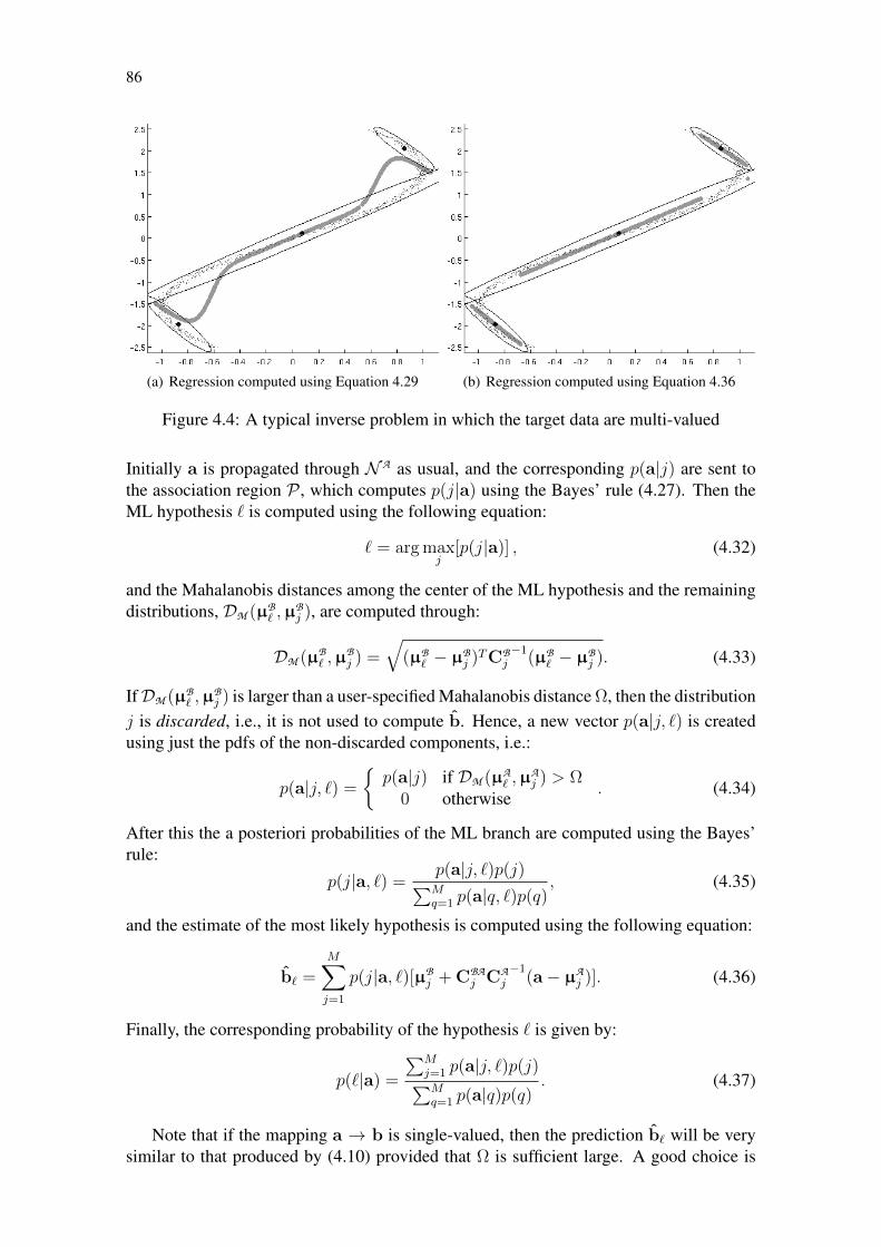
86
(a) Regression computed using Equation 4.29 (b) Regression computed using Equation 4.36
Figure 4.4: A typical inverse problem in which the target data are multi-valued
Initially a is propagated through N A as usual, and the corresponding p(a|j) are sent tothe association region P , which computes p(j|a) using the Bayes’ rule (4.27). Then theML hypothesis ` is computed using the following equation:
` = arg maxj
[p(j|a)] , (4.32)
and the Mahalanobis distances among the center of the ML hypothesis and the remainingdistributions, DM (µB
` ,µBj ), are computed through:
DM (µB` ,µ
Bj ) =
√(µB
` − µBj )TCB
j−1
(µB` − µB
j ). (4.33)
IfDM (µB` ,µ
Bj ) is larger than a user-specified Mahalanobis distance Ω, then the distribution
j is discarded, i.e., it is not used to compute b. Hence, a new vector p(a|j, `) is createdusing just the pdfs of the non-discarded components, i.e.:
p(a|j, `) =
p(a|j) if DM (µA
` ,µAj ) > Ω
0 otherwise. (4.34)
After this the a posteriori probabilities of the ML branch are computed using the Bayes’rule:
p(j|a, `) =p(a|j, `)p(j)∑Mq=1 p(a|q, `)p(q)
, (4.35)
and the estimate of the most likely hypothesis is computed using the following equation:
b` =M∑j=1
p(j|a, `)[µBj + CBA
j CAj−1
(a− µAj )]. (4.36)
Finally, the corresponding probability of the hypothesis ` is given by:
p(`|a) =
∑Mj=1 p(a|j, `)p(j)∑Mq=1 p(a|q)p(q)
. (4.37)
Note that if the mapping a → b is single-valued, then the prediction b` will be verysimilar to that produced by (4.10) provided that Ω is sufficient large. A good choice is

87
Ω = 5, because the probability that a point belonging to a distribution j falls outside aMahalanobis distance of five is≈ 5.7×10⁻⁷, and hence the influence of j over the currenthypothesis ` is negligible. In fact, a Mahalanobis distance of five is a common choice invisual applications that use Gaussian kernels as filters (HEINEN; ENGEL, 2009d,e). Inour experiments, described in the next chapters, we have set Ω = 6 to guarantee that themechanism described above does not influence the estimates computed in those regionswhere the target function is single-valued.
If we are estimating a sensory/motor modality a from b the procedure described abovewill be exactly the same – only the roles of a and b will be interchanged. Moreover, ifwe need to find out all possible answers for a given inverse problem, on the other hand,then the procedure above can be iterated using as the current (i.e., ML) hypothesis the dis-carded distribution with the largest a posteriori probability p(j|b). It is important to notethat this mechanism does not need to be used during learning because as p(j|z) is com-puted using both p(a|j) and p(b|j) then just the Gaussian units of the current branch havesignificant a posteriori probabilities, i.e., if we are informing all sensory/motor stimuli itis not possible to have multiple valid solutions.
Algorithm 4 presents the IGMN recalling algorithm that uses the mechanism de-scribed above, that is called general IGMN recalling algorithm to differentiate it fromthe special IGMN recalling algorithm presented in Algorithm 3. This algorithm returnsalmost the same predictions computed by the Algorithm 3 in single-valued regions (pro-vided that Ω ≥ 5), and in multi-valued regions the general algorithm will provide themost likely prediction instead of the average of all valid answers.
Algorithm 4 Summary of the general IGMN recalling algorithmfor all data a do
Activate the cortical region N Afor all neuron j dop(a|j) = N (a|µA
j ,CAj ) = 1
(2π)DA/2
√|CA
j |exp
−1
2(a− µA
j )TCAj−1
(a− µAj )
end forActivate the association region Pfor all neuron j do
p(j|a) =p(a|j) p(j)∑Mq=1 p(a|q) p(q)
end forCompute the a posteriori probabilities for branch of the ML hypothesis ` only` = arg maxj[p(j|a)]
DM (µB` ,µ
Bj ) =
√(µB
` − µBj )TCB
j−1
(µB` − µB
j )
p(j|a, `) =p(a|j, `)p(j)∑Mq=1 p(a|q, `)p(q)
Activate the cortical region N B to compute the estimates b` and CB`
for all neuron j doxBj = µB
j + CBAj CA
j−1
(a− µAj )
end forb` =
∑Mj=1 p(j|a, `) xB
j
CB` =
∑Mj=1 p(j|a, `)
CBj −CBA
j CAj−1CBAjT
+ ‖xBj − b`‖2
end for

88
Using the general recalling algorithm IGMN can solve the forward and inverse prob-lems using the same partially trained neural network even in regions where the targetfunction is multi-valued. To the best of our knowledge, IGMN is the first ANN modelendowed with this capability, although some possibilities have been pointed out in thecontext of Gaussian mixture models (BISHOP, 1995). Next section presents a detaileddescription of all configuration parameters used by IGMN and how to set them.
4.5 IGMN configuration parameters
IGMN has a total of eight configuration parameters. Three of them are related torestarting of the accumulators spj and can be configured as follows: spmax = 108, β = 0.8and γ = 0.5. These parameters are actually constants that have no influence in the IGMNperformance: they only prevent an eventual saturation of the corresponding accumulators.
The configuration parameters spmin and υmin are inherited from the IGMM stabilitycriterion. In IGMM they control the addition of new components and remove the spuriousones. In IGMN, on the other hand, they are used only to remove spurious components.As described in Subsection 2.5.3, a natural choice for spmin is D + 1, because accordingto Tråvén (1991) a minimum D+ 1 samples are required to obtain a nonsingular estimateof an unconstrained covariance matrix. The υmin parameter, on the other hand, can be setto any value larger than D + 1 such as 100 or 1000. Actually the only result of deletingspurious components is to speed up a little bit the ANN performance, because as thespurious components have low prior probabilities they don’t have any influence in theapproximation computed by IGMN.
The configuration parameter Ω, used to discard distributions of other branches (Sub-section 4.4), can always be set to Ω = 6. This parameter is actually a constant, becauseit can be kept fixed even in problems where the target function is single-valued. Anotherconfiguration parameter of IGMN is δ, used to set the initial radius of the covariancematrices, σK
ini. This parameter is not critical and can be set to any value in the interval0.005 ≤ δ ≤ 0.05 (its default value is 0.01). The only critical parameter of IGMN is themaximum approximation error εmax, that controls the level of generalization of the neuralnetwork. This parameter must be adjusted according to the maximum allowed error in agiven task. However, as the approximation error ε is normalized, εmax is usually set in theinterval 0.01 ≤ εmax ≤ 0.1.
Summing up, unless otherwise noted in all experiments described in this thesis theIGMN configuration parameters were set to spmax = 1018, β = 0.8, γ = 0.5, spmin =D + 1, υmin = 100, Ω = 6, δ = 0.01 and εmax = 0.05. We conclude that, althoughIGMN has many configuration parameters, just one of them must really be adjusted bythe user: the maximum approximation error εmax. Moreover, this parameter is easier toadjust, because in general the user knows the normalized approximation error acceptedin a given task. Next section concludes this chapter presenting a summary of the maincharacteristics and limitations of IGMN.
4.6 Final remarks
This chapter described the neural network model proposed in thesis, called IGMN, itsmain characteristics, mathematical basis, topology and learning algorithm. As describedbefore, IGMN extends the incremental Gaussian mixture model (IGMM), described inSection 2.5, in the following aspects:

89
• IGMN can be used in supervised function approximation rather than only in unsu-pervised clustering tasks;• It uses an error driven mechanism rather than the minimum likelihood criterion to
add new units;• IGMN can provide the confidence levels of its estimates;• The same partially trained neural network can be used to estimate either a and b
even when the target data are multi-valued;• The computational complexity is broken down by using separate covariance matri-
ces for distinct sensory/motor stimuli;• Equations 4.10 and 4.26 allow a multivariate representation without having to main-
tain and/or invert full variance/covariance matrices.
Moreover, most of these characteristics are not present in other neural network modelssuch as MLP, RBF and GRNN, which makes IGMN an useful tool for incremental func-tion approximation and on-line prediction tasks.
The main drawback of IGMN is that it is necessary to invert the covariance matricesCKj for each training sample (a,b, . . . ,k), and therefore its computational complexity is
O(NM(DADB . . . DS )log2 7). Subsection 2.5.6 presents some ways to reduce this com-plexity, such as to compute the inverse matrix C−1 directly using the method proposed bySato and Ishii (2000). Another way to reduce the computational complexity is to separatethe data features in more sensory/motor areas, thus dividing a big covariance matrix inmany matrices of smaller size. Although this may degrade the computed approximation(specially when all features are highly correlated), it is still a better solution than to con-sider all features as conditionally independent. Next chapter presents some experimentsperformed to evaluate IGMN in function approximation and prediction tasks.

90

91
5 FUNCTION APPROXIMATION USING IGMN
This chapter describes several experiments to evaluate the performance of IGMN infunction approximation and prediction tasks. The first set of experiments, described inSection 5.1, uses a sinusoidal data set to explore some basic aspects of the proposedmodel such as the advantages of the multivariate representation over the conditional in-dependence hypothesis, how the order of presentation of data affects the results and thesensibility of the proposed model to its configuration parameters. Section 5.2 describessome experiments in which the performance of IGMN is evaluated using a more complex,three-dimensional “Mexican hat” function. Section 5.3 describes how IGMN can be usedto predict both a and b from the same trained neural network, i.e., how IGMN can be usedto solve the forward and inverse problems at the same time. Section 5.4 presents someexperiments in which IGMN is used to identify a nonlinear plant originally proposed byNarendra and Parthasarathy (1990). Section 5.5 demonstrates how IGMN can be usedfor predicting the future values of a cyclic time series. Finally, Section 5.6 presents somefinal remarks about these experiments.
In practically all experiments presented in this chapter the performance of IGMN iscompared against other ANN models, such as MLP and GRNN, available in the MAT-LAB Neural Network (NN) Toolbox software. The IGMN prototype was implementedin the C ANSI computer programming language. It uses POSIX threads to allow a par-allel execution in multi-processed platforms. The inverse matrices and determinants arecomputed using the LU decomposition algorithm presented in Press et al. (1992) whosecomputational complexity is Dlog2 7. The computer platform used in all experiments is aDell Optiplex 755, equipped with an Intel(R) Core(TM)2 Duo CPU 2.33GHz processor,64 bits architecture, 1.95GB of RAM memory, GPU Intel and operating system UbuntuLinux 10.04 LTS of 64 bits.
5.1 Sinusoidal data set
This section describes a set of experiments to evaluate the performance of IGMN usinga simply and easy to visualize two-dimensional function. More specifically, the data setused in this set of experiments is composed by N = 1000 data samples generated usingthe following function:
b = sin(a) + ε, (5.1)
where a is drawn from a uniform distribution in the interval [−π, π] and ε is an inde-pendent Gaussian noise vector with mean µε = 0 and standard deviation σε = 0.05.Figure 5.1 shows this data set, where the black dots represent the (a, b) sample pairs andthe gray line represents the target function, i.e., b = sin(a) without noise.

92
Figure 5.1: Sinusoidal data set of size N = 1000 corrupted with Gaussian noise
Next subsections describe some experiments using this sinusoidal data set to evaluatemany aspects of the IGMN architecture such as: the advantages of a multivariate repre-sentation, how the order of presentation of data affects the results and the sensibility ofIGMN to its configuration parameters εmax and δ. Moreover, IGMN is compared withother connectionist approaches such as MLP, RBF and GRNN.
5.1.1 Standard × multivariate representation
The first experiment of this chapter is devised to compare the performance of IGMNusing a complete multivariate representation (Equation 4.10) against the assumption ofconditional independence among domains (4.9) used in the previous IGMN version pre-sented in Heinen and Engel (2010a; 2010b). To perform this experiment we have imple-mented two distinct versions of IGMN:
• Standard: assumes that the cortical regions are conditionally independent (i.e., thecortical regions are not correlated) and estimates the missing stimuli using (4.9);• Multivariate: assumes a full multivariate hypothesis and estimates the missing
stimuli using (4.10).
Therefore we have used both IGMN versions for learning the sinusoidal data setshown in Figure 5.1 using different settings of the εmax parameter. Table 5.1 shows theresults obtained in this experiment. In this experiment the δ parameter was set to δ = 0.01(its default value) and the training data were presented to the neural network in ascendingorder of a. As IGMN does not have any random initialization and/or decision, it is notnecessary to repeat each experiment many times (the results are always identical for thesame data set and configuration).
Each row on Table 5.1 represents a pair of experiments performed using a specificsetting of the εmax parameter. The first column indicates the εmax setting used in the cor-responding pair of experiments. The following columns show, respectively, the NRMSerror, the number of neurons (M ) added to each region during training and the time re-quired for learning the sinusoidal data set using the corresponding εmax setting. Columns2, 3, and 4 correspond to the standard IGMN version and columns 5, 6 and 7 correspondto the multivariate version of IGMN.
Observing Table 5.1 many important conclusions can be drawn from this experiment.First, the performance of the standard and multivariate versions of IGMN is quite good,

93
Table 5.1: Comparison between the standard and multivariate versions of IGMNStandard version Multivariate version
εmax NRMS M Time NRMS M Time0.2500 0.105653 12 0.010s 0.079194 3 0.000s0.1000 0.032439 18 0.015s 0.040956 8 0.005s0.0750 0.026288 24 0.020s 0.028581 7 0.010s0.0500 0.023269 30 0.030s 0.023555 29 0.050s0.0250 0.022063 57 0.075s 0.022111 57 0.080s0.0100 0.022004 134 0.355s 0.022203 140 0.430s0.0075 0.022024 173 0.630s 0.022099 173 0.800s
because using the original function b = sin(a) to compute d (the desired value) the NRMSerror is 0.024596. In fact, as the NRMS error is computed using the following equation:
NRMS =RMS
max(d)−min(b)
and the root mean square (RMS) error is given by the square root of the mean square error(MSE):
RMS =√MSE
MSE =1
N
N∑n=1
(di − bi)2,
then the expected NRMS error will be ≈ 0.025 because the noise vector has a standarddeviation σε = 0.05 and max(b) − min(b) ≈ 2. Therefore we can suppose that thebest setting of εmax is about 0.05 because it is supposed that the instantaneous normalizederror ε will be bellow RMS× 2 ≈ 0.05 for 98% of the training samples (this suppositionis based on the fact that a Mahalanobis distance of two defines a contour encompassingapproximately 98% of the training samples). Of course if the noise level is not known itis not possible to configure εmax using this heuristic.
Observing Table 5.1 it can be noticed that in fact the best value of εmax is ≈ 0.05,because using lower values the neural network tries without success to reduce the erroradding more neurons to each region. Nevertheless, it can be noticed that even using 173neurons the proposed model does not suffer from overfitting (HAYKIN, 2008; PEREIRA;RAO, 2009), because (4.10) computes b as a soft interpolation among the Gaussian centersweighted by the posterior probabilities. Hence the Gaussian neurons added exclusivelyto model the noise will have low a posteriori probabilities and will not affect significantlythe predictions (it is supposed that the noise is Gaussian, has zero mean and the extremevalues are infrequent).
Another interesting conclusion drawn from this experiment is that both IGMN ver-sions achieve the global optimum using εmax = 0.05 and approximately 30 neurons ineach region, but using high εmax values (e.g., 0.075) the multivariate version requires lessneurons to achieve the same performance of the standard version. To understand why thisoccurs Figures 5.2 and 5.3 show the regression curves of the standard and multivariateversions of IGMN using εmax = 0.075 and εmax = 0.025, respectively. In this figure, theGaussian components are represented by ellipses whose width is equivalent to a Maha-lanobis distance of two, and the mean of each distribution is shown by solid circles in thecenter of the respective ellipses. It can be noticed that IGMN creates some Gaussian units
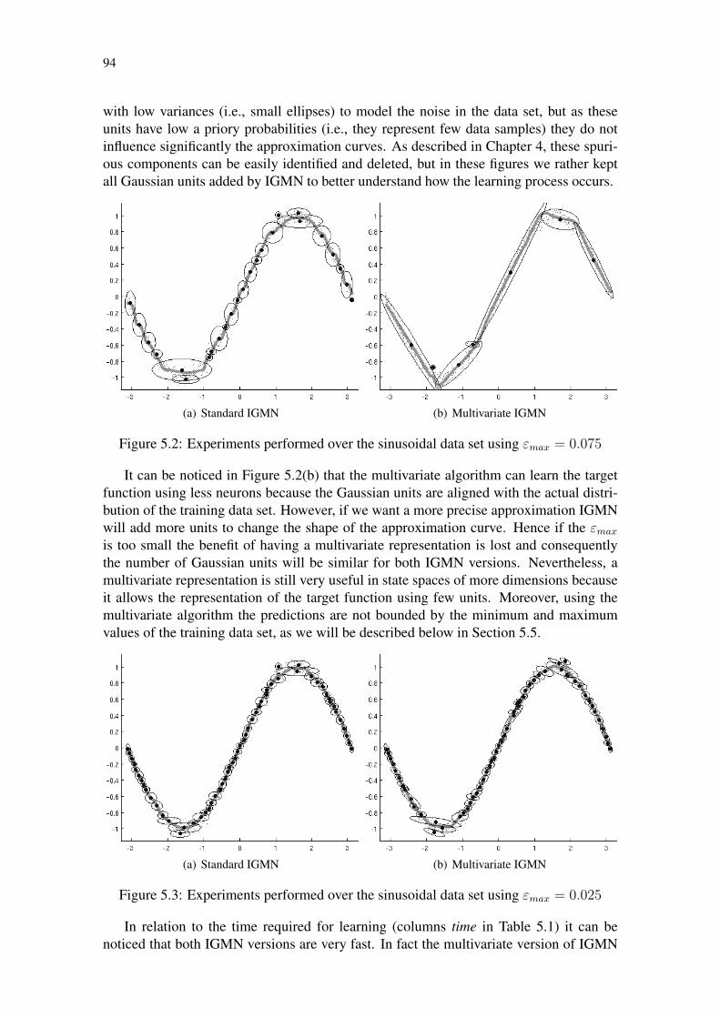
94
with low variances (i.e., small ellipses) to model the noise in the data set, but as theseunits have low a priory probabilities (i.e., they represent few data samples) they do notinfluence significantly the approximation curves. As described in Chapter 4, these spuri-ous components can be easily identified and deleted, but in these figures we rather keptall Gaussian units added by IGMN to better understand how the learning process occurs.
(a) Standard IGMN (b) Multivariate IGMN
Figure 5.2: Experiments performed over the sinusoidal data set using εmax = 0.075
It can be noticed in Figure 5.2(b) that the multivariate algorithm can learn the targetfunction using less neurons because the Gaussian units are aligned with the actual distri-bution of the training data set. However, if we want a more precise approximation IGMNwill add more units to change the shape of the approximation curve. Hence if the εmaxis too small the benefit of having a multivariate representation is lost and consequentlythe number of Gaussian units will be similar for both IGMN versions. Nevertheless, amultivariate representation is still very useful in state spaces of more dimensions becauseit allows the representation of the target function using few units. Moreover, using themultivariate algorithm the predictions are not bounded by the minimum and maximumvalues of the training data set, as we will be described below in Section 5.5.
(a) Standard IGMN (b) Multivariate IGMN
Figure 5.3: Experiments performed over the sinusoidal data set using εmax = 0.025
In relation to the time required for learning (columns time in Table 5.1) it can benoticed that both IGMN versions are very fast. In fact the multivariate version of IGMN

95
has learned the sinusoidal data set composed by N = 1000 data samples in less than asecond even using εmax = 0.0075, i.e., using 173 multivariate neurons in each region. Ofcourse in problems of higher dimensionality the multivariate version will require moretime to invert the larger covariance matrices.
Although these results are very impressive, the NRMS error computed over the train-ing data set is not a good estimator of the approximation error because it can be influencedby overfitting. Hence, this experiment was repeated using the 10-fold cross validationmethod (HAYKIN, 2008), in which the learning data set is randomly divided into 10 sub-sets. The learning process is repeated 10 times using a different subset for testing (i.e., tocompute the generalization error) and the remaining 9 subsets for learning. The boxplotgraphs1 of Figure 5.4 show the results computed using the 10-fold cross validation proce-dure. The configuration parameters used in this experiment are δ = 0.01 and εmax = 0.05.
(a) NRMS error (b) Number of neurons
Figure 5.4: Comparison between standard and multivariate regression
It can be noticed in Figure 5.4(a) that the confidence intervals are overlapped, andtherefore it is considered that both algorithms have the same generalization performance.The average NRMS error is 0.028379 for the standard algorithm and 0.028501 for themultivariate algorithm. Observing Figure 5.4(b), on the other hand, it can be noticedthat the multivariate algorithm is really more parsimonious than the standard algorithm:the average number of neurons added during learning is 32.9 for the standard algorithmand 26.3 for the multivariate algorithm. Throughout this section we will still evaluatethe performance of both versions of IGMN, but in the next sections we will use just themultivariate version of IGMN because its representational power is superior than that ofthe standard algorithm.
Another interesting conclusion that can be drawn from the experiment above is thefact that different implementations of IGMN (standard and multivariate) can approximatethe target function with almost the same precision, using the same configuration param-eters but different number of neurons in each region. This occurs due to the error-drivenmechanism used by IGMN that simply adds so many neurons as necessary to achievethe specified approximation level, no matter what kind of neuron is used. This a strongpoint of the current version of IGMN, because using the τnov parameter to control the ap-
1A boxplot is a convenient way statistical tool for graphically depicting groups of numerical data throughtheir five-number summaries: the smallest observation (sample minimum), lower quartile, median, upperquartile, largest observation (sample maximum) and outliers (MASSART et al., 2005).

96
proximation level each IGMN version would be carefully adjusted to achieve the desiredperformance. In fact the τnov parameter is related to the shape and size of the Gaussianunits, not to the approximation level of the target function. Of course in clustering tasksthe number and the shape of the Gaussian distributions is essential, but in regression thegoal is to achieve the required precision no matter how many neurons are used.
5.1.2 Assessing the sensibility of the δ parameter
In the previous experiments we have changed the εmax parameter to see how IGMNis affected by this configuration parameter, but we have set δ = 0.01. In this section wepresent some experiments in which the εmax is set to 0.05 (its best configuration accordingto Table 5.1) and the δ parameter is varied in order to assess its sensibility. Table 5.2 showsthe results obtained in this experiment using both versions of IGMN and the 10-fold crossvalidation procedure.
Table 5.2: Assessing the sensibility of the δ parameterStandard Multivariate
δ NRMS M NRMS M0.0010 0.042843 41.0 0.031196 70.70.0025 0.033888 65.8 0.028613 51.40.0050 0.028703 46.4 0.028325 34.70.0075 0.029878 34.4 0.027900 32.00.0100 0.026773 29.7 0.026554 27.00.0250 0.026055 29.7 0.025388 24.90.0500 0.027096 38.0 0.027186 43.70.0750 0.045344 170.2 0.039672 94.6
For better understanding these results, Figures 5.5 and 5.6 show the boxplot graphscomputed over this experiment using the standard and multivariate versions of IGMN,respectively. It can be noticed that although extreme values of δ can degrade the approxi-mation and/or require many Gaussian units, using 0.005 ≤ δ ≤ 0.05 the results are prac-tically the same using both the standard and multivariate algorithms, and this indicatesthat IGMN is not sensible to this parameter. Moreover, as σini is computed using δ andthe minimum and maximum values of each feature (Equation 2.35), then the δ parameteris not affected by resizing and normalization procedures.
Actually the δ parameter can always be set to 0.01 without problems, as will bedemonstrated throughout this thesis. In the remaining experiments of this section δ willbe kept fixed at 0.01, but in Section 5.4 we will again vary δ to demonstrate that it isreally uncritical. Next section describes an experiment performed to verify if the order ofpresentation of data affects the results produced by IGMN.
5.1.3 Ordered × shuffled data sets
In the previous experiments the training data were always presented in ascending or-der of a, i.e., the training data set was ordered. The next experiment is devised to verifyif the order of presentation of data significantly affects the approximation computed byIGMN. Hence, we will perform two experiments using both versions of IGMN each, thefirst experiment presenting the training data in ascending order of a (as in the previousexperiments) and the second presenting the data in a random order. To simplify our ex-

97
(a) NRMS error (b) Number of neurons (M )
Figure 5.5: Assessing the sensibility of δ – Standard IGMN algorithm
(a) NRMS error (b) Number of neurons (M )
Figure 5.6: Assessing the sensibility of δ – Multivariate IGMN algorithm
planation, we will use the term ordered data set to refer to the presentation of data inascending order of a and shuffled data set to refer to the presentation of data in a randomorder, although the data samples themselves are the same in both data sets. Figures 5.7and 5.8 show the results obtained in these experiments computed using the 10-fold crossvalidation procedure. The IGMN configuration parameters were set in these experimentsto εmax = 0.05 and δ = 0.01.
It can be noticed in Figure 5.7 that the order of presentation of data affects stronglythe standard algorithm. In fact the NRMS error computed over the shuffled data set isalmost twice the error computed over the ordered data set. Moreover, the number ofGaussian units added during learning is significantly larger when the shuffled data set isused. Observing the boxplot graphs shown in Figure 5.8, on the other hand, we can noticethat the multivariate algorithm is not strongly affected by the order of presentation of data,i.e., the differences between the results computed over each data set are not statisticallysignificant (the confidence intervals overlap).
Based on the boxplot graphs of Figure 5.8 we can affirm that the multivariate algo-rithm is not affected by the order of presentation of data when εmax = 0.05, but we don’tknow if this robustness stands using other settings of εmax. To answer this question thisexperiment was repeated using other εmax settings, and the results computed using the10-fold cross validation procedure are shown in Table 5.3. Based on these results we can

98
(a) NRMS error (b) Number of neurons
Figure 5.7: Ordered × shuffled data sets – Standard algorithm
(a) NRMS error (b) Number of neurons
Figure 5.8: Ordered × shuffled data sets – Multivariate algorithm
now affirm that the multivariate algorithm is really robust to the order of presentation ofdata, because as can be noticed in Table 5.3 the results (number of units added duringlearning and NRMS error) computed over both data sets are similar. But the standardIGMN algorithm, on the other hand, is really affected by the order of presentation of data,but the differences are reduced as the εmax parameter is lowered.
The explanation why just the standard algorithm is affected by the order of presenta-tion of data is the following. When the multivariate algorithm is used the Gaussian unitsrapidly assume the shape and size of the training data, and thus the state space is rapidlycovered and clustered according to the actual distribution of these training data. Hence,after the presentation of some training patterns each data vector falls into the most likelycluster (i.e., a Gaussian distribution that is close to the actual distribution of data in thatregion of the state space) no matter in which order these training vectors are presented.Figure 5.9 illustrates this situation, where the Gaussian units obtained using the orderedand shuffled data sets are shown (in this experiment εmax was set to 0.05). Observing thisfigure we notice that the Gaussian units added during learning are not exactly the same forboth data sets, but the resulting approximation and the number of neurons are practicallythe same in both experiments.

99
Table 5.3: Comparison between ordered shuffled data setsStandard Multivariate
εmax Data set NRMS M NRMS M0.075 Ordered 0.029947 22.6 0.031741 7.40.075 Shuffled 0.059026 27.6 0.029370 12.50.050 Ordered 0.026773 29.7 0.026554 27.00.050 Shuffled 0.048697 37.0 0.028602 27.70.025 Ordered 0.025927 54.9 0.025516 57.50.025 Shuffled 0.036486 59.5 0.025882 58.5
(a) Ordered data set (b) Shuffled data set
Figure 5.9: Gaussian units added during learning – Multivariate algorithm
Using the standard algorithm, on the other hand, many small clusters are created tomodel the regions of the state space where the target function is not parallel to the coor-dinate axis, as can be noticed in Figure 5.2(a) above. If the training data are presentedin order the Gaussian units will be added evenly to cover the state space, as shows Fig-ure 5.10(a). But if the training data is presented in a random order then many Gaussianunits will be created irregularly, as shows Figure 5.10(b). We can notice in this figurethat some units assume shapes and sizes that are not similar to the distribution of thetraining data. Moreover, many spurious components are created to model the noise andsome distributions become very large, as is clearly seen in Figure 5.10(b). These ir-regular distributions created by the standard algorithm difficult the approximation of thetarget function, and therefore the results are worse when the training data is presentedin a random order. Nevertheless, for the kind of application we are interested in (incre-mental function approximation) the training data generally arrive in a specific order (e.g.,when the data consist on sensory readings of a mobile robot navigating through an envi-ronment), and therefore the standard IGMN algorithm can be used in these applicationswithout problems.
Based on these experiments we conclude that the standard algorithm is significantlyaffected by the order or presentation of data, but this does not occur when we are usingthe multivariate algorithm, i.e., the multivariate algorithm is relatively robust to the orderof presentation of data. As described in Chapter 4 the main drawback of the multivariaterepresentation is that it has a higher computational cost which is bearable only if this rep-resentation provides a real benefit to the learning algorithm. But based on the experiments
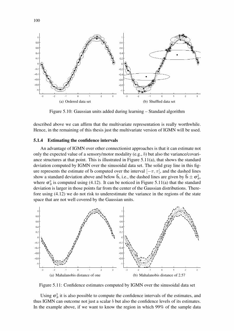
100
(a) Ordered data set (b) Shuffled data set
Figure 5.10: Gaussian units added during learning – Standard algorithm
described above we can affirm that the multivariate representation is really worthwhile.Hence, in the remaining of this thesis just the multivariate version of IGMN will be used.
5.1.4 Estimating the confidence intervals
An advantage of IGMN over other connectionist approaches is that it can estimate notonly the expected value of a sensory/motor modality (e.g., b) but also the variance/covari-ance structures at that point. This is illustrated in Figure 5.11(a), that shows the standarddeviation computed by IGMN over the sinusoidal data set. The solid gray line in this fig-ure represents the estimate of b computed over the interval [−π, π], and the dashed linesshow a standard deviation above and below b, i.e., the dashed lines are given by b± σ2
B ,where σ2
B is computed using (4.12). It can be noticed in Figure 5.11(a) that the standarddeviation is larger in those points far from the center of the Gaussian distributions. There-fore using (4.12) we do not risk to underestimate the variance in the regions of the statespace that are not well covered by the Gaussian units.
(a) Mahalanobis distance of one (b) Mahalanobis distance of 2.57
Figure 5.11: Confidence estimates computed by IGMN over the sinusoidal data set
Using σ2B it is also possible to compute the confidence intervals of the estimates, and
thus IGMN can outcome not just a scalar b but also the confidence levels of its estimates.In the example above, if we want to know the region in which 99% of the sample data

101
will fall, for instance, we can plot contours with a Mahalanobis distance of 2.57, i.e,b± 2.57σ2
B , as shows Figure 5.11(b). The confidence estimates computed by IGMN arevery useful to make decisions, for instance, because they allow us to plan the actions usingnot just an estimate of b but also the confidence intervals. These confidence estimates arevery useful in real time applications operating in hazardous environments, because in thiskind of task we cannot take the risk of making a wrong decision. Next subsection presentsa comparison among IGMN and other ANN models.
5.1.5 Comparison with other ANN models
This section presents some experiments performed to compare IGMN with other ex-isting connectionist approaches. To perform a comparison using the sinusoidal data setwe have selected the following ANN models:
• Multi-layer Perceptron (MLP) trained using the Resilient Propagation (RPROP)algorithm (RIEDMILLER; BRAUN, 1993);• MLP trained by the Levenberg-Marquardt (LM) algorithm (HAGAN; MENHAJ,
1994), which is a second order method that learns faster than the standard back-propagation algorithm and RPROP;• Radial basis functions (RBF) network (POWELL, 1985, 1987a,b) created using the
‘newrb’ method of the MATLAB Neural Network Toolbox (this method incremen-tally adds neurons until an specified goal is achieved);• General regression neural network (GRNN) (SPECHT, 1991).
These neural network models were chosen because they are well known and avail-able in the MATLAB Neural Network Toolbox software. Moreover, they are good rep-resentatives of the class of connectionist methods used for function approximation andprediction. Another possibility would be some of the improved GRNN models presentedin Section 3.8, but as most part of these models just reduces the number of pattern units(i.e., the generalization level is not improved) we decided to use only the standard GRNNin these experiments. To make the comparison fair, we performed an exhaustive trial anderror search to find out the best configuration of each ANN model listed below:
• MLP: a single hidden layer with 8 hidden neurons;• RBF: goal (minimum MSE) = 0.0025 and spread (σ) = 0.25;• GRNN: spread (σ) = 0.05;• IGMN: εmax = 0.05 and σ = 0.01.
The stop criterion used in these experiments for the MLP and RBF models was theearly stopping criterion based on the best generalization epoch. Table 5.4 shows the re-sults obtained in these experiments. The first column presents the ANN model. Thefollowing columns show, respectively, the number of hidden/pattern units, the NRMS er-ror computed using the 10-fold cross validation procedure, the average number of trainingepochs and the time required to perform each replication, i.e. 1/10 of the time required bythe entire 10-fold cross validation procedure. To facilitate our comparison, the last rowson Table 5.4 show the results obtained using both IGMN versions.
It is important to notice that the number of hidden/pattern units (the second column onTable 5.4) is just informative, because the ANN models are based on different principles(MLP is a global model, RBF has local receptive fields, GRNN is non-parametric, etc.)and therefore it is not possible to evaluate the model complexity (number of free parame-ters) based on this information. Similarly, the time required for learning (last column on

102
Table 5.4) is not a fair measure of the computational complexity because it depends onthe implementation details of each architecture. Nevertheless, we can notice that IGMNis very fast, because even using full covariance matrices it performed each replication inless than 50 milliseconds.
Table 5.4: Comparative among ANN models using the sinusoidal data setANN model Units NRMS Epochs TimeMLP – RPROP 8.0 0.031384 107.1 5.444sMLP – LM 8.0 0.024866 20.3 3.196sRBF 24.5 0.025631 24.5 6.673sGRNN 1000.0 0.025569 1.0 0.481sIGMN – Standard 29.7 0.026773 1.0 0.028sIGMN – Multivariate 27.0 0.026554 1.0 0.041s
Figure 5.12 shows a boxplot graph comparing the NRMS error obtained in each exper-iment. Observing this figure and Table 5.4 we can notice that all ANN models (exceptingMLP – RPROP) have a similar performance (the confidence intervals overlap). There-fore, we can affirm that IGMN is a very good regression tool because it achieves a similarlevel of generalization using an incremental architecture and a single scan over the train-ing data. Moreover, using IGMN we don’t need to inform the number of hidden neuronsneither to fine-tune many configuration parameters (actually it is much easier to configureIGMN that the other ANN models).
Figure 5.12: Comparative of the NRMS error among ANNs – sinusoidal data set
5.2 Approximating the “Mexican hat” function
In the previous experiments we have used a training data set composed by just twodata features, a and b. The next experiment uses a three-dimensional data set composedby N = 5000 data samples given by:
b = sin(a1)/a1 sin(a2)/a2, (5.2)
were a1 and a2 are randomly chosen in the interval [−10, 10]. Figure 5.13(a) shows thetarget surface, also known as “Mexican hat”. The IGMN net used to learn this data set hastwo cortical regions: N A , composed by two data features (a1 and a2), andN B , composed

103
by a single feature (b). This data set was randomly divided into two subsets, called train-ing and testing data sets, each of them composed by 2500 data samples. Moreover, thetraining data was presented to IGMN in a random order (i.e., the data set was shuffled).
(a) Target surface (b) εmax = 0.1 (c) εmax = 0.075
(d) εmax = 0.05 (e) εmax = 0.025 (f) εmax = 0.01
Figure 5.13: Approximating the “Mexican hat” function using IGMN
To assess the sensibility of IGMN to εmax over this data set we have repeated thisexperiment using different configurations of εmax, and the results obtained in this experi-ment are shown in Table 5.5. The first row shows the configuration of the εmax parameter.The following rows show, respectively, the NRMS error, number of neurons added duringlearning (M ) and the learning time. The δ parameter was kept fixed at 0.01, but the resultsare practically the same using δ in the interval 0.005 ≤ δ ≤ 0.05.
Table 5.5: Approximating the “Mexican hat” function using IGMNεmax 0.1 0.075 0.05 0.025 0.01NRMS 0.071302 0.067699 0.065824 0.051815 0.014288M 19 25 37 83 184Time 0.088s 0.104s 0.188s 0.656s 2.292s
Table 5.5 shows that the NRMS error is reduced as the εmax parameter is decreased,whilst the number of neurons added during learning is increased. Using εmax = 0.01, forinstance, the NRMS error is just 0.014288, but 184 neurons are added to each region dur-ing learning. If εmax ≈ 0 then the approximation error will be almost zero (remember thatthis data set is noise-free), but a huge number of neurons will be added during learning.Just for illustration purposes, Figures 5.13(b) to 5.13(f) show the surface approximated byIGMN using each εmax setting. We can notice in these figures that using just 21 neurons

104
(Figure 5.13(b)) the proposed model is able to learn the general structure of the targetsurface, and using 184 neurons (Figure 5.13(f)) the approximated surface is quite good.
Using a MLP neural network trained with the Levenberg-Marquardt (LM) algorithmand 20 hidden neurons, the average NRMS error computed over the testing data set was0.015265 (we needed to repeat this experiment 10 times due to the random initializationof the synaptic weights in a MLP network), and the time required for learning was 20.633seconds. However, using MLP we had to perform an exhaustive search to find out the bestnumber of hidden neurons. Using GRNN with σ = 1.0, on the other hand, the NRMSerror was 0.017395 and the learning time was 0.189 seconds. As said before, the numberof neurons added by GRNN is equal to the number of pattern neurons, i.e., 2500 patternneurons in this case.
Based on this experiment we conclude that IGMN can learn a three-dimensional sur-face with arbitrary precision, and the number of neurons added during learning is propor-tional to the required approximation level. Next section describes how IGMN can be useto estimate both a and b using the same neural network.
5.3 Estimating both a and b
In the previous experiments we have always used a specific sensory/motor signal (e.g.,a) to predict another (e.g., b), i.e., IGMN has learned and predicted just the forwardfunction. However, we can use the same partially trained IGMN network (as IGMN canlearn continuously we never consider that the training process has finished) to predict boththe forward and the inverse function, i.e., to predict both b from a and a from b as well.To demonstrate this IGMN capability, initially we describe an experiment using a data setof size N = 1000 generated by the following function:
b = tanh(a) + ε, (5.3)
where tanh(·) is the hyperbolic tangent function, ε is an independent Gaussian noisevector with mean µε = 0 and standard deviation σε = 0.025 and a is drawn from auniform distribution in the interval [−e, e], where e = 2.718281828 is the Euler number.Figure 5.14(a) shows this data set, where the gray line represents the target function, i.e.,b = tanh(a) without noise. An interesting point about this function is that both f(·) andf(·)−1 are mathematical functions in the interval [−e, e].
This data set was learned by IGMN as usual: Ω was set to 6, εmax to 0.05, δ to0.01, and 6 Gaussian units were added during learning, as shows Figure 5.14(b). Afterlearning this neural network was used to estimate b from a, as shows the solid gray lineon Figure 5.15(a). The estimates of b were computed by propagating a into the corticalregionN A , computing p(j|a) in the association region P and estimating b on regionN B .
We can notice in Figure 5.15(a) that the approximation performed by IGMN is quitegood: the NRMS error computed over b is 0.013664, which is almost σε/[max(b) −min(b)], i.e., the expected NRMS error. Moreover, this same neural network can be usedto estimate a from b without retraining, as shows the gray line in Figure 5.15(b). We cannotice in this figure that the approximation of the inverse function performed by IGMN isalso good: the NRMS error computed over a is 0.033378. The main difference occurs atthe top-right extremum, because in that region the distribution is almost parallel to the aaxis.

105
(a) Generated data set and target function (b) Gaussian units added during learning
Figure 5.14: Hyperbolic tangent data set corrupted with noise
(a) Estimating b from a (b) Estimating a from b
Figure 5.15: Estimating both a and b in a hyperbolic tangent data set
This experiment has demonstrated that IGMN can approximate both a and b if f(·)and f(·)−1 are functions in R, but this constraint is not really necessary. If f(·)−1 is afunction in a more limited domain, for instance, IGMN can also predict a in the regionswhere f(·)−1 is a mathematical function. To demonstrate this functionality we have useda data set composed by N = 500 data samples generated using the following cubic func-tion:
b =a3
5+
3a2
4− 3a− 2 (5.4)
where a is randomly chosen in the interval [−8, 6]. Figure 5.16(a) shows this data set andthe Gaussian units added by IGMN during learning. For estimating the forward functiona → b in the domain R, we can use any connectionist approach such as MLP, RBF,GRNN and IGMN, of course. Figure 5.16(b) shows the regression of f(·) in the interval[−8, 6] performed by IGMN. The NRMS error computed over b is 0.009131, and theconfiguration parameters were set to εmax = 0.025, δ = 0.01 and Ω = 6 (actually in allexperiments of this thesis Ω was set to 6).
However, if we need to estimate the inverse function f(·)−1 using a connectionistapproach the procedure is more complicated, because f(·)−1 leads to many solutions in

106
(a) Cubic data set and the corresponding neurons (b) Estimating the forward function using IGMN
Figure 5.16: Experiments performed over the cubic data set
the interval [−4.2, 9.25]. If we use a connectionist approach such as MLP or GRNN toestimate the inverse function, the result will be similar to that presented in Figure 5.17(a),where the approximation is very poor in the interval [−4.2, 9.25], i.e., the predictionsare far from the target function in that region. Nevertheless, outside this interval theapproximation of f(·)−1 using a MLP is quite good, as can be seen in Figure 5.17(a).
(a) Regression performed by MLP (b) ML regression performed by IGMN
Figure 5.17: Estimating both a from b in the cubic data set
Using a traditional ANN model such as MLP and GRNN this can be tackled only byrestricting the domain in which the inverse function is evaluated, but using a more com-plex, high-dimensional data set, sometimes it is difficult to identify the regions wheref(·)−1 is a mathematical function. Using IGMN, on the other hand, the solution isstraightforward: we use the approach described in Section 4.4 to identify this situationand tackle it appropriately. As described in Section 4.4, the solution for this problem canbe: (i) to predict a only in those regions where f(·)−1 is a function; (ii) to return themost likely hypothesis in the conflict points and (iii) to return all possible hypotheses andthe corresponding a posteriori probabilities. Figure 5.17(b) shows the approximation per-formed by IGMN using the second alternative, i.e., returning the most likely hypothesisof a. According to Bishop (1995), the most likely hypothesis is a good solution in many
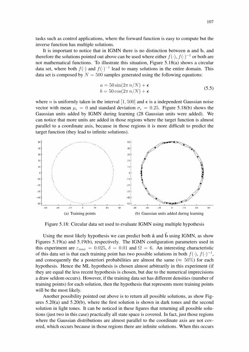
107
tasks such as control applications, where the forward function is easy to compute but theinverse function has multiple solutions.
It is important to notice that in IGMN there is no distinction between a and b, andtherefore the solutions pointed out above can be used where either f(·), f(·)−1 or both arenot mathematical functions. To illustrate this situation, Figure 5.18(a) shows a circulardata set, where both f(·) and f(·)−1 lead to many solutions in the entire domain. Thisdata set is composed by N = 500 samples generated using the following equations:
a = 50 sin(2π n/N) + εb = 50 cos(2π n/N) + ε
(5.5)
where n is uniformly taken in the interval [1, 500] and ε is a independent Gaussian noisevector with mean µε = 0 and standard deviation σε = 0.25. Figure 5.18(b) shows theGaussian units added by IGMN during learning (28 Gaussian units were added). Wecan notice that more units are added in those regions where the target function is almostparallel to a coordinate axis, because in those regions it is more difficult to predict thetarget function (they lead to infinite solutions).
(a) Training points (b) Gaussian units added during learning
Figure 5.18: Circular data set used to evaluate IGMN using multiple hypothesis
Using the most likely hypothesis we can predict both a and b using IGMN, as showFigures 5.19(a) and 5.19(b), respectively. The IGMN configuration parameters used inthis experiment are εmax = 0.025, δ = 0.01 and Ω = 6. An interesting characteristicof this data set is that each training point has two possible solutions in both f(·), f(·)−1,and consequently the a posteriori probabilities are almost the same (≈ 50%) for eachhypothesis. Hence the ML hypothesis is chosen almost arbitrarily in this experiment (ifthey are equal the less recent hypothesis is chosen, but due to the numerical imprecisionsa draw seldom occurs). However, if the training data set has different densities (number oftraining points) for each solution, then the hypothesis that represents more training pointswill be the most likely.
Another possibility pointed out above is to return all possible solutions, as show Fig-ures 5.20(a) and 5.20(b), where the first solution is shown in dark tones and the secondsolution in light tones. It can be noticed in these figures that returning all possible solu-tions (just two in this case) practically all state space is covered. In fact, just those regionswhere the Gaussian distributions are almost parallel to the coordinate axis are not cov-ered, which occurs because in those regions there are infinite solutions. When this occurs

108
(a) Estimating b from a (b) Estimating a from b
Figure 5.19: Estimating both a and b on the circular data set
IGMN returns the solution that is nearest to the center of the ML hypothesis, which isgenerally the best solution because it represent an “average answer”.
(a) Estimating b from a (b) Estimating a from b
Figure 5.20: Returning multiple solutions for the circular data set
Of course if we need to take an action, for instance, we must decide what hypothesisis the most suitable for a given situation. As said before, in the circular data set bothhypotheses are equiprobable, and hence the a posteriori probabilities do not help us totake a decision. But if we are using the data set shown in Figure 5.16(a), on the otherhand, the ML hypothesis will be that associated with the highest “probability mass”, andtherefore we will tend to choose the ML hypothesis because it represents the most commonanswer among the valid ones, i.e., the hypothesis that is more supported by the trainingdata.
Based on these experiments we conclude that IGMN can be used to predict both theforward and the inverse functions even when they are not functions in the mathematicalsense. Moreover, these predictions can be made using the same partially trained neuralnetwork, i.e., it is not necessary to have distinct neural networks for the forward and the in-verse models. To the best of our knowledge IGMN is the first neural network model whichhas this capability, although in the context of Gaussian mixture models some possibili-

109
ties have been pointed out before by Bishop (1995) and Ghahramani and Jordan (1994a;1994b) (but not using an incremental Gaussian mixture model).
5.4 Estimating the outputs of a nonlinear plant
The next experiment consists in identifying a nonlinear plant originally proposed byNarendra and Parthasarathy (1990) for the control of nonlinear dynamical systems usingMLP neural networks. This plant is assumed to be of the form:
yp(k + 1) = f [yp(k), yp(k − 1), yp(k − 2), u(k), u(k − 1)], (5.6)
where yp(k + 1) is the next time sample of the plant output, yp(k) is the current output,yp(k− 1) and yp(k− 2) are delayed time samples of the output, u(k) is the current input,u(k − 1) is the previous input, and the unknown function f(·) has the form:
f [x1,x2,x3,x4,x5] =x1x2x3x5(x3 − 1) + x4
1 + x22 + x2
3
. (5.7)
In Narendra and Parthasarathy (1990) this plant was identified using a MLP neuralnetwork composed by five neurons in the input layer, 20 neurons in the first hidden layer,10 neurons on the second hidden layer and a single neuron in the output layer. Thisneural network was trained using the standard backpropagation algorithm for 100000steps using a random input signal uniformly distributed in the interval [−1, 1] and a stepsize of η = 0.25. During the identification procedure (i.e., the learning process) a series-parallel model was used (Figure 5.21(b) (NARENDRA; PARTHASARATHY, 1990)), inwhich the output of the plant values (i.e., the desired answers) were used in the delay unitsyp(k − 1) and yp(k − 2). After identification the performance of the model was assessedusing a parallel model (Figure 5.21(a) (NARENDRA; PARTHASARATHY, 1990)), inwhich the actual neural network outputs are fed into the delay units. The identified plant(i.e., the trained neural network) was tested using the following function as input:
u(k) =
sin(2πk/250) if k ≤ 5000.8 sin(2πk/250) + 0.2 sin(2πk/25) if k > 500
(5.8)
(a) Parallel identification model (b) Series-parallel identification model
Figure 5.21: Identification models
Figure 5.22(a), reproduced from Narendra and Parthasarathy (1990), shows the resultsobtained in that experiment. It can be noticed that the Narendra’s model was able to

110
identify this plant and to predict the next output yp(k + 1) even using a random inputsignal (rather than Equation 5.8) during learning, which shows that the neural networkwas able to learn the input/out behavior of the given plant after 100,000 learning steps.
(a) Identification using the Narendra’s model (b) Identification using GRNN
Figure 5.22: Identification of the nonlinear plant using some previous approaches
In Specht (1991) a GRNN network is used to approximate the function f(·) above.In that experiment the identification procedure was carried out for 1000 time steps usinga random input signal uniformly distributed in the interval [−1, 1], and the spreadingparameter was set to σ = 0.315. Figure 5.22(b), reproduced from Specht (1991), showsthe results obtained in that experiment. Using GRNN 1000 pattern units were used torepresent this plant (one for each random input signal used to identify the plant).
Unfortunately in Specht (1991) the approximation error computed using the testingfunction (5.8) is not informed, and thus we reproduced that experiment 10 times usingthe original conditions (a standard GRNN network with σ = 0.315) and different ran-dom input signals in each replication. Figure 5.23(a) shows the best identification (i.e.,the replication in which the NRMS error is the smaller) performed by GRNN. The aver-aged NRMS error computed over 10 replications was 0.053267, and 0.213 seconds werenecessary to perform each replication.
To compare the performance of IGMN against the ANN models described above, wehave repeated this experiment using the same conditions described above, i.e.:
• A series-parallel model (Figure 5.21(b)) for training and a parallel model (Fig-ure 5.21(a)) for testing;• The identification procedure was carried out for 1000 time steps using a random
input signal uniformly distributed in the interval [−1, 1];• The training data was presented in a random order (the training data set is shuffled);• After learning the identified model was tested using inputs given by Equation 5.8;• The whole experiment was repeated 10 times using different random input signals
in each replication.
Figure 5.23(b) shows the identification performed by IGMN using default parameters,i.e., εmax = 0.05 and δ = 0.01. Observing Figure 5.23(b) we can notice that the identifi-cation performed by IGMN is superior than those performed by MLP and GRNN (Figures

111
(a) Identification performed by GRNN (b) Identification performed by IGMN
Figure 5.23: Identification of a nonlinear plant using 1000 training samples
5.22(a) and 5.22(b), respectively). The average NRMS error computed over 10 replica-tions was 0.037, 19 neurons were added by IGMN during learning and 0.089 secondswere spent in each replication.
Table 5.6: Assessing the sensibility of IGMN to the εmax parameterSetting of εmax 0.1 0.075 0.050 0.025 0.010NRMS error 0.0474 0.0399 0.0370 0.0394 0.0304Neurons (M ) 8.30 12.60 19.10 38.10 80.40Learning time 0.055s 0.089s 0.095s 0.125s 0.285s
To assess the sensibility of IGMN to the εmax parameter, this experiment was re-peated using δ = 0.01 and varying the value of the εmax in the interval [0.01, 0.1]. Ta-ble 5.6 shows the results obtained in this experiment (averaged over 10 replications), andFigures 5.24(a) and 5.24(b) show the boxplot graphs of the NRMS error and the num-ber of units added during learning, respectively. It can be noticed in these figures thatεmax = 0.05 is a good choice, because it allows a good compromise between the modelcomplexity (number of neurons) and the approximation level (NRMS error).
(a) NRMS error (b) Number of neurons
Figure 5.24: Assessing the sensibility of IGMN to the εmax parameter
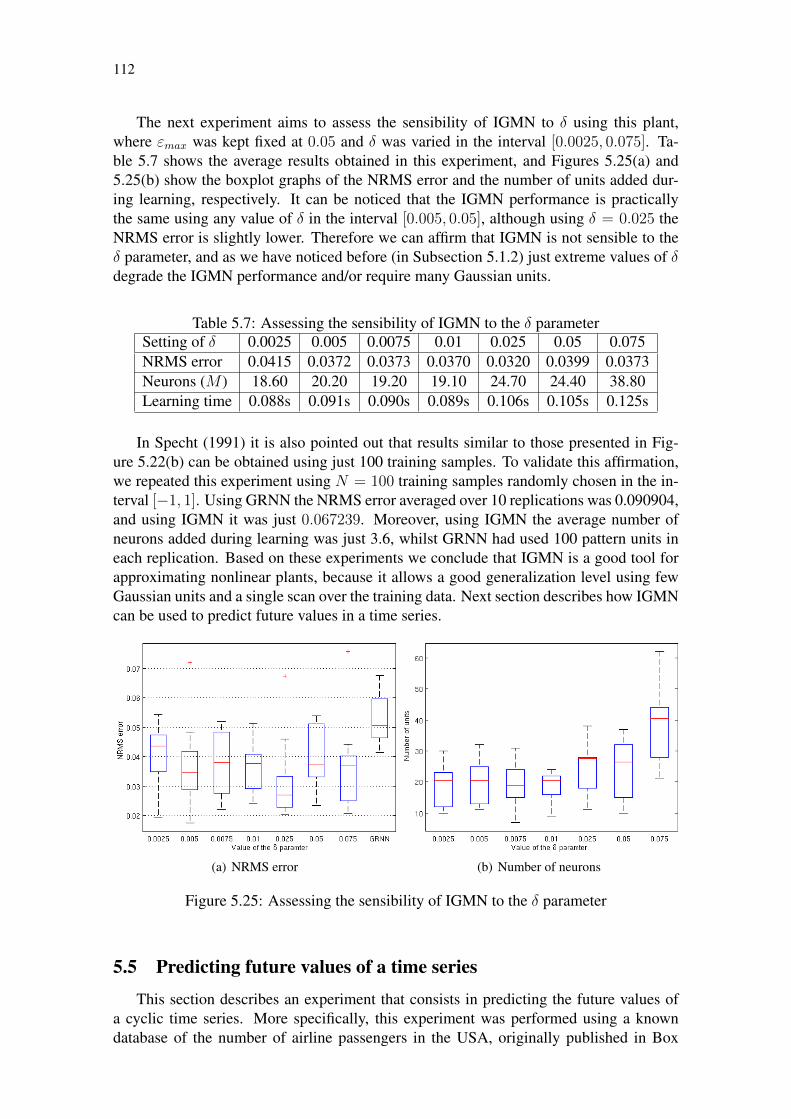
112
The next experiment aims to assess the sensibility of IGMN to δ using this plant,where εmax was kept fixed at 0.05 and δ was varied in the interval [0.0025, 0.075]. Ta-ble 5.7 shows the average results obtained in this experiment, and Figures 5.25(a) and5.25(b) show the boxplot graphs of the NRMS error and the number of units added dur-ing learning, respectively. It can be noticed that the IGMN performance is practicallythe same using any value of δ in the interval [0.005, 0.05], although using δ = 0.025 theNRMS error is slightly lower. Therefore we can affirm that IGMN is not sensible to theδ parameter, and as we have noticed before (in Subsection 5.1.2) just extreme values of δdegrade the IGMN performance and/or require many Gaussian units.
Table 5.7: Assessing the sensibility of IGMN to the δ parameterSetting of δ 0.0025 0.005 0.0075 0.01 0.025 0.05 0.075NRMS error 0.0415 0.0372 0.0373 0.0370 0.0320 0.0399 0.0373Neurons (M ) 18.60 20.20 19.20 19.10 24.70 24.40 38.80Learning time 0.088s 0.091s 0.090s 0.089s 0.106s 0.105s 0.125s
In Specht (1991) it is also pointed out that results similar to those presented in Fig-ure 5.22(b) can be obtained using just 100 training samples. To validate this affirmation,we repeated this experiment using N = 100 training samples randomly chosen in the in-terval [−1, 1]. Using GRNN the NRMS error averaged over 10 replications was 0.090904,and using IGMN it was just 0.067239. Moreover, using IGMN the average number ofneurons added during learning was just 3.6, whilst GRNN had used 100 pattern units ineach replication. Based on these experiments we conclude that IGMN is a good tool forapproximating nonlinear plants, because it allows a good generalization level using fewGaussian units and a single scan over the training data. Next section describes how IGMNcan be used to predict future values in a time series.
(a) NRMS error (b) Number of neurons
Figure 5.25: Assessing the sensibility of IGMN to the δ parameter
5.5 Predicting future values of a time series
This section describes an experiment that consists in predicting the future values ofa cyclic time series. More specifically, this experiment was performed using a knowndatabase of the number of airline passengers in the USA, originally published in Box

113
et al. (1976). The data consist of the monthly quantity of passengers measured over 12consecutive years, between 1949 and 1960, summing up 144 samples. The goal of thisexperiment is the prediction of the number of passengers for the subsequent four years,i.e, the next 48 data records. This database has been focus of a competition for time seriesprediction in the 25th International Symposium on Forecasting2, held in 2005.
A critical decision in this experiment is the choice of the number of entries, D, to beused in the neural network. This decision is critical due to the reduced number of samplesin the sample data set. As D increases, the number of training/testing samples decreases.The relationship between the number of samples and entries is given as follows:
Q = N −D,
where Q is the is the number of samples available for training. If D = 12, for instance,the records of the previous year, X = xn−D+1, xn−D+2, . . . , xn−1, xn, are used to pre-dict the next record xn+1 and Q = 132 samples are available for learning and testing.In Camargo and Engel (2005) it is pointed out that using a MLP network the best pos-sible configuration is given by using two hidden neurons and D = 48 entries (i.e., theprediction is based on the previous four years), which results in 96 samples availablefor learning and testing. We have also performed several preliminary experiments usingdifferent configurations in a MLP network, and these experiments confirmed that the con-figuration pointed out above is the best possible for a MLP neural network trained usingthe Levenberg-Marquardt (LM) algorithm.
Using the best configuration pointed out above, i.e., a MLP network with 48 inputs,two hidden neurons and a single output, we have repeated this experiment 10 times usingdifferent random initializations, and the best replication is shown in Figure 5.26(a). It canbe noticed in this figure that the MLP neural network does not learn correctly the growingtendency in the time series. Moreover, this is the only really good result obtained in the 10replications. The most common results are similar to that shown in Figure 5.26(b), wherethe prediction of the next 48 values is poor. Besides, in some replications the results aresimilar to that present in Figure 5.26(c), where the neural network did not learn even thetraining data set. The time required for learning is about 2 seconds using the MATLABNN Toolbox.
This experiment points out two well-known problems of the backpropagation algo-rithm and its variants (e.g., RPROP and LM): (i) the obtained results depend on the ini-tialization of the random weights; and (ii) the learning algorithm is susceptible to localminima. Using less entries in the neural network, e.g.,D = 18, the results are even worse,as can be seen in Figure 5.26(d), that is the best replication using this configuration.
In Camargo (2010) a progressive enhancement neural model is used to select the mostrelevant features and to retrain the neural network using just these features. Figure 5.27,reproduced from Camargo (2010), shows the results obtained by Camargo using this tech-nique. The results shown in Figure 5.27 were sent to the competition for time series pre-diction in the 5th International Symposium on Forecasting, and was awarded among thethree best works in this competition (CAMARGO; ENGEL, 2005). Unfortunately theCamargo’s technique is not on-line nor incremental: it needs to retrain the neural networkmany times using a batch-mode algorithm.
In the next experiment IGMN was used to predict the subsequent 48 values of this timeseries. In this experiment we have used the number of entries pointed out above (D = 48),
225th IFS, San Antonio, USA – http://www.upcomillas.es/presim/documentos/recu_09.pdf
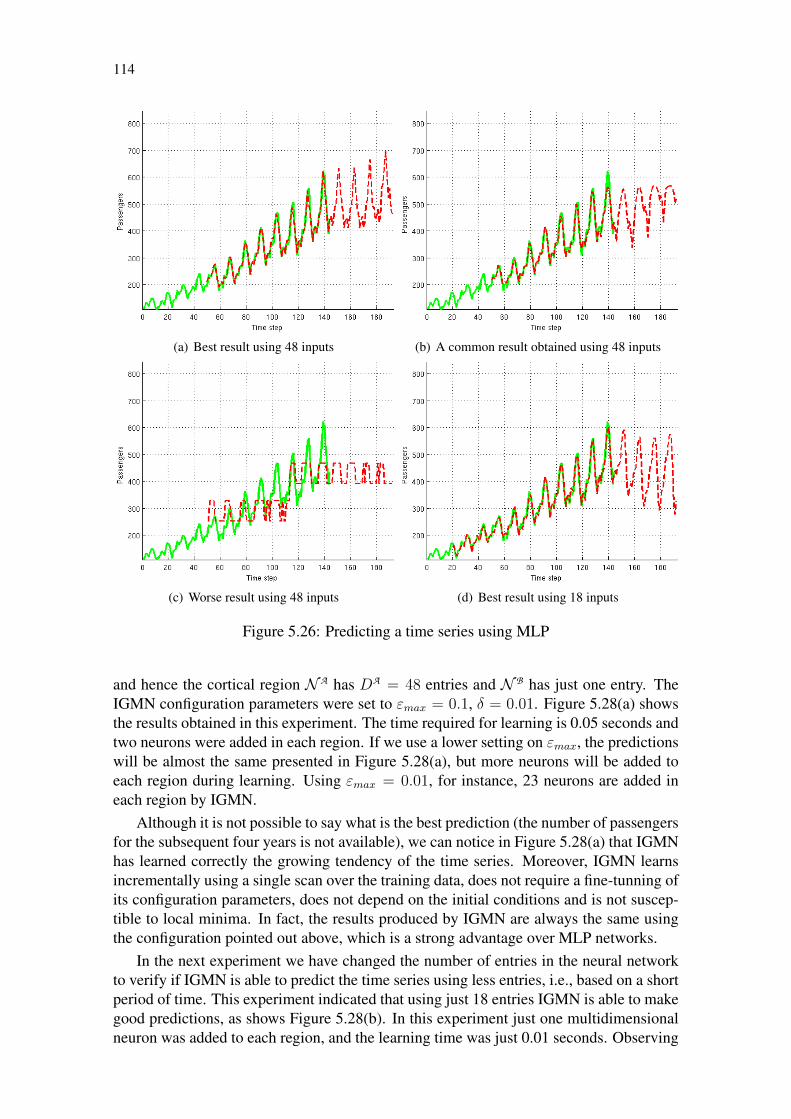
114
(a) Best result using 48 inputs (b) A common result obtained using 48 inputs
(c) Worse result using 48 inputs (d) Best result using 18 inputs
Figure 5.26: Predicting a time series using MLP
and hence the cortical region N A has DA = 48 entries and N B has just one entry. TheIGMN configuration parameters were set to εmax = 0.1, δ = 0.01. Figure 5.28(a) showsthe results obtained in this experiment. The time required for learning is 0.05 seconds andtwo neurons were added in each region. If we use a lower setting on εmax, the predictionswill be almost the same presented in Figure 5.28(a), but more neurons will be added toeach region during learning. Using εmax = 0.01, for instance, 23 neurons are added ineach region by IGMN.
Although it is not possible to say what is the best prediction (the number of passengersfor the subsequent four years is not available), we can notice in Figure 5.28(a) that IGMNhas learned correctly the growing tendency of the time series. Moreover, IGMN learnsincrementally using a single scan over the training data, does not require a fine-tunning ofits configuration parameters, does not depend on the initial conditions and is not suscep-tible to local minima. In fact, the results produced by IGMN are always the same usingthe configuration pointed out above, which is a strong advantage over MLP networks.
In the next experiment we have changed the number of entries in the neural networkto verify if IGMN is able to predict the time series using less entries, i.e., based on a shortperiod of time. This experiment indicated that using just 18 entries IGMN is able to makegood predictions, as shows Figure 5.28(b). In this experiment just one multidimensionalneuron was added to each region, and the learning time was just 0.01 seconds. Observing

115
Figure 5.27: Predicting the time series using Camargo’s model
Figure 5.28(b) we can notice that IGMN correctly predicts the time series based on thelast 18 months with an accuracy higher than that provided by MLP (Figure 5.26(d)).
After this we have used GRNN to learn this time series and to compare its perfor-mance against IGMN. After an exhaustive search for the best adjusting of the spreadingparameter σ, we have found out that the best setting is given using σ = 0.075. The train-ing data were also normalized in the interval [−1, 1], which is an requirement of GRNNbecause the Parzen kernels have the same width in each direction (SPECHT, 1991). Fig-ures 5.29(a) and 5.29(b) shows the results obtained using a GRNN net with 48 and 18entries, respectively.
We notice in Figure 5.29 that even using the best possible configuration GRNN can-not learn the growing tendency of the time series, and using other configurations and/orwithout normalizing the training data the results are even worse. This occurs becauseaccording to Specht (1991) in GRNN “the estimate is bounded by the minimum and max-
(a) Prediction using 48 delayed time units (b) Prediction using 18 delayed time units
Figure 5.28: Predicting the time series using IGMN

116
(a) Prediction using 48 delayed time units (b) Prediction using 18 entries
Figure 5.29: Predicting the time series using GRNN (σ = 0.075)
imum of the observations”, which prevents it of learning the growing tendency in the timeseries. Similarly, if we use IGMN with the standard algorithm, a result similar to thatpresented in Figure 5.29(a) is obtained, no matter how long time we spend trying to ad-just the configuration parameters. This experiment points out that only using multivariateGaussian units we can predict correctly this time series. Therefore, we conclude that therepresentational power of the multivariate algorithm really provides a real benefit to theneural network, and as we have pointed out before in Section 5.1 the higher computationalcost of the multivariate representation is worthwhile because it allow us to predict a cyclictime series with growing tendency better than other ANN models.
Another important aspect about predicting time series is that sometimes the predic-tion itself is not enough. In fact, as the behavior of many systems is chaotic, it is veryuseful to compute the confidence limits of the forecasts, because they may allow us tomake a better decision based on the confidence intervals, for instance. As described be-fore, predicting the confidence limits using IGMN is straightforward – we just need tocompute the variance at b using (4.12) and use this variance to compute other estimatorssuch as the confidence intervals. Figures 5.30(a) and 5.30(b) show the 95% confidenceintervals computed by IGMN over the time series described above using 48 and 18 en-tries, respectively. We can notice that both experiments lead to similar results, but using48 entries the confidence interval is narrow, what indicates that the confidence is higherwhen more information is used (i.e., the past experience is more deeply exploited by theneural network) to predict the time series.
Based on these experiments we can conclude that IGMN is a very good tool for learn-ing time series, because it allow us to predict a cyclic time series in a robust and efficientmanner. Moreover, it captures correctly the growing tendency of the time series and isnot susceptible to local minima. Next section presents some final conclusions about theexperiments described in this chapter.
5.6 Final remarks
This chapter has presented several experiments performed using the proposed neuralnetwork model in function approximation and prediction tasks. These experiments haveexemplified the main characteristics of IGMN, hence showing that it is a very suitable ma-

117
(a) confidence intervals using 48 entries (b) Confidence intervals using 18 entries
Figure 5.30: 95% confidence intervals computed by IGMN
chine learning tool for on-line prediction and regression tasks. In fact, the results obtainedin these experiments have demonstrated that: (i) IGMN learns very fast using a singlescan over training data; (ii) it does not depend on the initial conditions nor is susceptibleto local minima (the results are always identical for the same data set and configuration);(iii) the neural network architecture is incrementally defined; (iv) it is not necessary tofine-tune the configuration parameters to obtain good results; (v) the multivariate repre-sentation is robust to the order or presentation of data; (vi) the predictions are not boundedby the minimum and maximum values of the training data set; (vii) IGMN can providethe confidence levels of its estimates; (viii) the same neural network can be used to esti-mate both the forward and the inverse functions; (ix) IGMN can provide good estimateseven when either f(·) or f(·)−1 are not mathematical functions; (x) its performance in theexperiments described above is equivalent or even superior than those presented by otherconnectionist solutions such as MLP and GRNN; (xi) the learning algorithm is relativelyrobust to the overfitting problem; and (xii) IGMN can be successfully used in many prob-lems such as estimating the outputs of a nonlinear plant or predicting the future values ofa time series with growing tendency. Next chapter presents some experiments in whichIGMN is used in more complex machine learning tasks such as reinforcement learningand robotic control.

118

119
6 ROBOTICS AN OTHER RELATED TASKS
Last chapter has described many experiments, using artificial (synthetic) datasets, thatdemonstrated the representational power and learning performance of IGMN. This chap-ter describes the second contribution of this thesis, which is the use of IGMN in practicalapplications such as reinforcement learning and robotics. The main goal of these exper-iments is to validate the proposed model in real applications and/or using real data andalso to demonstrate its suitability in many potential applications that require incrementallearning and real time performance. This chapter is structured as follows. Section 6.1 dis-cusses the use of IGMN for incremental concept formation (ENGEL; HEINEN, 2010a,b;HEINEN; ENGEL, 2010e,f), which is an important task in machine learning and robotics.Section 6.2 shows how IGMN can be used to compute the control actions for a mobilerobot performing a wall following behavior (HEINEN; ENGEL, 2010a,b,d). Section 6.3demonstrates the suitability of IGMN for computing the inverse kinematics in a gait con-trol task using a simulated legged robot (HEINEN; OSÓRIO, 2009, 2008, 2007b). Sec-tion 6.4 presents the use of IGMN as a function approximator in reinforcement learning(RL) algorithms (HEINEN; ENGEL, 2010g,a, 2009a,c). Finally, Section 6.5 describesa new feature-based mapping algorithm (HEINEN; ENGEL, 2011, 2010c,f), based onIGMN, which represents the environment using multivariate GMMs rather than grid cellsor line segments. Great part of these experiments has been published in the correspondingpapers cited above using a previous (i.e., the standard) IGMN version, but in this chapterwe have performed these experiments again using the most recent (i.e, the multivariate)IGMN algorithm, which leads to better results than those presented in the papers men-tioned above.
6.1 Incremental concept formation
One of our primary motivations in developing IGMN was to tackle problems like thoseencountered in autonomous robotics. To be more specific, let us consider the so calledperceptual learning, which allows an embodied agent to understand the world (BUR-FOOT; LUNGARELLA; KUNIYOSHI, 2008). Here an important task is the detectionof concepts such as “corners”, “walls” and “corridors” from the sequence of noisy sensorreadings (e.g., sonar data) of a mobile robot. The detection of these regularities in dataflow allows the robot to localize its position and to detect changes in the environment(THRUN; BURGARD; FOX, 2006).
Although concept formation has a long tradition in machine learning literature, in thefield of unsupervised learning, most methods assume some restrictions in the probabilis-tic modeling (GENNARI; LANGLEY; FISHER, 1989) which prevent their use in on-linetasks. The well known k-means algorithm (MACQUEEN, 1967; TAN; STEINBACH;

120
KUMAR, 2006) (Section 2.2), for instance, represents a concept as a mean of a subsetor cluster of data. In this case, each data point must deterministically belong to one con-cept. The membership of a data point to a concept is decided by the minimum distanceto the means of the concepts. To compute the means, all data points belonging to everyconcept are averaged using a fixed number of concepts along all the learning process.For learning probabilistic models, a very used approach is the batch-mode EM algorithm(DEMPSTER; LAIRD; RUBIN, 1977) (Section 2.3), which follows a mixture distribu-tion approach for probabilistic modeling. Like k-means, this algorithm requires that thenumber of concepts be fixed and known at the start of the learning process. Moreover, theparameters of each distribution are computed through the usual statistical point estima-tors, a batch-mode approach which considers that the complete training set is previouslyknown and fixed (TAN; STEINBACH; KUMAR, 2006).
These restrictions make the k-means and EM algorithms not suitable for on-line con-cept formation, because in this kind of task usually each data point is just instantaneouslyavailable, i.e., the learning system needs to build a model, seen as a set of concepts of theenvironment, incrementally from data flows. The neural network model proposed in thisthesis, on the other hand, is able to learn from data flows in an incremental (new conceptscan be added by demand) and on-line (it does not require that the complete training set bepreviously known and fixed) way, which makes it a good solution for concept formationin on-line robotic tasks. Moreover, unlike the traditional neural network models (e.g.,MLP and GRNN), the IGMN hidden neurons are not “black boxes”, and thus the Gaus-sian units can be interpreted as representations of the input space, i.e., high level concepts(HEINEN; ENGEL, 2010e). The remaining of this section is organized as follows: Sub-section 6.1.1 presents some related work about concept formation, and Subsection 6.1.2describes how IGMN can be used to build high-level concepts incrementally from dataflows.
6.1.1 Related work
In the past different approaches were presented to create high level concepts fromsonar data in robotic tasks. As a typical example of these approaches, Nolfi and Tani (1999)proposed a hierarchical architecture to extract regularities from time series, in whichhigher layers are trained to predict the internal state of lower layers when such statessignificantly change. In this approach, the segmentation was cast as a traditional errorminimization problem (HAYKIN, 2008), which favors the most frequent inputs, filteringout less frequent input patterns as being “noise”. The result is that the system recognizesslightly differing walls, that represent frequent input patterns, as distinct concepts, butis unable to detect corridors or corners that are occasionally (infrequently) encountered.Moreover, this algorithm has scarce means to handle the stability-plasticity dilemma andto appropriately model the data.
Figure 6.1(a) shows the environment used by Nolfi and Tani (1999) to validate theirapproach, where it is considered the case of a mobile robot that performs a wall followingbehavior in an environment composed by two rooms joined by a short corridor. In thisfigure the straight lines represent the walls and the full circle represents a cylindricalobject. The circle on the left-bottom side represents the robot and the trace on the terrainrepresents the trajectory of the robot during a few laps in the environment. The roboticplatform used in this experiment is a simulated Khepera robot. This robot has a circularshape with a diameter of 55mm, a height of 30mm, and a weight of 70g. It is supportedby two wheels and two small Teflon balls. The wheels are controlled by two DC motors

121
with an incremental encoder. The robot is provided with eight infrared proximity sensorsthat can detect obstacles within a range of about 3cm.
(a) Training environment and data acquisition (b) Segmentations performed during one lap
Figure 6.1: Results obtained using the Nolfi and Tani’s model in an environment com-posed by two rooms joined by a short corridor
Figure 6.1(a), reproduced from Nolfi and Tani (1999), shows the segmentation per-formed by the Nolfi and Tani’s model during one lap in the environment. The full circle,empty circle, and full square indicate, respectively, which of the three segmentation unitsis active in a given cycle. The state of the segmentation units is displayed only when a newsegmentation occurs (i.e. when the state changes). The arrows indicate the direction ofthe robot when the corresponding segmentation occurs. This experiment was performedusing an Elman’s network (ELMAN, 1990) with 10 input units (which encode the stateof the eight infrared sensors of the robot and the speed of the two motors), 3 hidden units(which detect the states of the environment), and 8 output units (which encode the stateof the infrared sensors at time t+1). The main drawbacks of this approach are: (i) it re-quires that the number of concepts (i.e., hidden units) be fixed and known at the start ofthe learning process; and (ii) the learning algorithm is off-line and requires several scansover the training data to converge (in fact the neural network using in this experiment wastrained for 100000 epochs).
Focusing in change detection, Linåker and Niklasson (2000a; 2000b) proposed anadaptive resource allocating vector quantization (ARAVQ) network, which stores mov-ing averages of segments of the data sequence as vectors allocated to output nodes ofthe network. New model vectors are incorporated to the model if a mismatch betweenthe moving average of the input signal and the existing model vectors is greater than aspecified threshold, and a minimum stability criterion for the input signal is fulfilled. Fig-ure 6.2, reproduced from Linåker (2003), shows the results obtained using the ARAVQnetwork and the Khepera robot simulator (MICHEL, 1996), in the same environmentshown in Figure 6.1(a). The main advantage of this approach over the Nolfi and Tany’smodel is that the ARAVQ network requires a single scan over the training data to con-verge. Moreover, it can add hidden neurons (i.e., to create new concepts) incrementallyfrom data flows.
Although the ARAVQ network has been used in some robotic tasks (LINÅKER;JACOBSSON, 2001; BAKKER; LINÅKER; SCHMIDHUBER, 2002; BAKKER et al.,2003; LINÅKER, 2003; HOLLAND; GOODMAN, 2003; STENING; JACOBSSON;ZIEMKE, 2005), like other distance-based clustering algorithms its induced model isequivalent to a set of equiprobable spherical distributions sharing the same variance, what
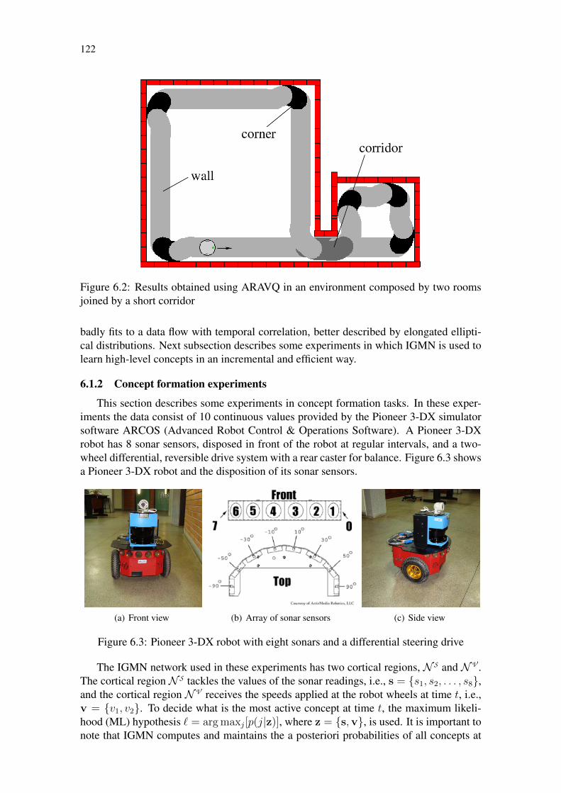
122
Figure 6.2: Results obtained using ARAVQ in an environment composed by two roomsjoined by a short corridor
badly fits to a data flow with temporal correlation, better described by elongated ellipti-cal distributions. Next subsection describes some experiments in which IGMN is used tolearn high-level concepts in an incremental and efficient way.
6.1.2 Concept formation experiments
This section describes some experiments in concept formation tasks. In these exper-iments the data consist of 10 continuous values provided by the Pioneer 3-DX simulatorsoftware ARCOS (Advanced Robot Control & Operations Software). A Pioneer 3-DXrobot has 8 sonar sensors, disposed in front of the robot at regular intervals, and a two-wheel differential, reversible drive system with a rear caster for balance. Figure 6.3 showsa Pioneer 3-DX robot and the disposition of its sonar sensors.
(a) Front view (b) Array of sonar sensors (c) Side view
Figure 6.3: Pioneer 3-DX robot with eight sonars and a differential steering drive
The IGMN network used in these experiments has two cortical regions, N S and N V .The cortical region N S tackles the values of the sonar readings, i.e., s = s1, s2, . . . , s8,and the cortical region N V receives the speeds applied at the robot wheels at time t, i.e.,v = v1, v2. To decide what is the most active concept at time t, the maximum likeli-hood (ML) hypothesis ` = arg maxj[p(j|z)], where z = s,v, is used. It is important tonote that IGMN computes and maintains the a posteriori probabilities of all concepts at

123
each time, and hence it can be used in applications such as the so called multi-hypothesistracking problem in robotic localization domains (FILLIAT; MEYER, 2003; THRUN;BURGARD; FOX, 2006). The configuration parameters used in the following experi-ments are δ = 0.1 and τnov = 0.01 (as the main goal in concept formation is to identifynatural groupings in the input space, we have decided to use in this experiment the τnovparameter to adjust the model complexity rather than the εmax parameter). It is importantto say that no exhaustive search was performed to optimize the configuration parameters.
The first experiment was accomplished in an environment composed of six corridors(four external and two internal), and the robot performed a complete cycle in the externalcorridors. Figure 6.4 shows the segmentation of the trajectory obtained by IGMN whenthe robot follows the corridors of this environment. IGMN created four probabilisticunits, corresponding to the concepts “corridor” (1: plus sign), “wall at right” (2: circle),“corridor / obstacle front” (3: asterisk) and “curve at left” (4: cross). The symbols inthe trajectory of Figure 6.4 represent the ML hypothesis in each robot position, and theblack arrow represents the robot starting position and direction. More details about thisexperiment can be found at Engel and Heinen (2010a).
Figure 6.4: Segmentation obtained by IGMN in six corridors experiment
The next experiment was performed in a more complex environment, composed bytwo different sized rooms connected by a short corridor. This environment was inspiredin those used by Linåker and Niklasson (2000a; 2000b) (Figure 6.1(a) above). Figure 6.5shows the segmentation performed by IGMN in this experiment. IGMN has created sevenclusters, corresponding to the concepts ”wall at right” (1: plus sign), ”corridor” (2: circle),”wall at right / obstacle front” (3: asterisk), ”curve at left” (4: cross), ”bifurcation /obstacle front” (5: square), ”bifurcation / curve at right” (6: five-pointed star) and ”wallat left / curve at right” (7: hexagram).
Comparing these experiments, it can be noticed that some similar concepts, like “curveat left” and “obstacle front”, were discovered in both experiments, although these envi-ronments are different (the environment shown in Figure 6.4 has many corridors whilst

124
Figure 6.5: Segmentation obtained by IGMN in the two rooms experiment
that one shown in Figure 6.5 has two large rooms and just one short corridor). This pointsout that concepts extracted from a data flow corresponding to a specific sensed environ-ment are not restricted to this environment, but they form an alphabet that can be reusedin other contexts. This is a useful aspect, that can improve the learning process in morecomplex environments.
As described above, the main goal in concept formation is to identify natural group-ings in the input space, which are represented by IGMN using its Gaussian units. There-fore, in this kind of task the estimation/prediction capabilities of IGMN are not necessary(in fact, this experiment can be performed using IGMM as well). Nevertheless, theseestimation/prediction capabilities can be used to compute the motor actions for a robotperforming a wall following behavior, for instance, as is shown in the next subsection.
6.2 Estimating the desired speeds in a mobile robotics application
In the experiments described in the previous section the main goal was to identifynatural groupings in the input space, which were represented by the IGMN Gaussian units,and therefore the IGMN estimation/prediction capabilities were not used. In this sectionwe will use these estimation/prediction capabilities to compute the desired actions (i.e.,the wheel speeds) for a mobile robot performing a wall following behavior in a simulatedenvironment. These experiments are relevant because in robotic control tasks usually itis not possible to predict all situations that occur in the real world, and hence the robotneeds to learn from experience while interacting with the environment.
In a previous experiment, presented in Heinen and Engel (2010a), Equation 4.9 wasused to estimate the desired speeds in the same environment described above (Figure 6.5)and using a IGMN neural network with two cortical regions, N S and N V and seven

125
Gaussian units added by the minimum likelihood criterion. Figure 6.6(a) shows the resultsobtained in this previous experiment, where the x axis corresponds to the time index of thesensor readings (the training database is composed by 2070 data samples) and the y axiscorresponds to the difference between the right and left motor speeds, i.e., yd(t) = v1−v2.A positive value in yd(t) corresponds to a left turn in the robot trajectory and a negativevalue corresponds to a right turn. The solid gray line in Figure 6.6(a) represents thedesired yd(t) values and the dashed black line represents the difference between the actualIGMN outcomes, i.e.: yo(t) = v1 - v2. It is important to say that the region N V has sizeDV = 2, i.e., the difference yo(t) was computed just to improve the visualization inFigure 6.6(a).
(a) Using a previous (standard) IGMN version (b) Using the current (multivariate) IGMN version
Figure 6.6: Difference between the speeds of the right and left motors of the robot whileit is fallowing the trajectory shown in Figure 6.5.
Observing Figure 6.6(a) we can notice that the standard IGMN version was able to ap-proximate the desired output with a reasonable accuracy (the NRMS error was 0.050373),using few Gaussian units (just seven) and no memory of past perceptions and actions (e.g.,no recurrent connections nor delay units). The main differences between yd(t) and yo(t)are in the extremes, i.e., the approximation performed by IGMN is smoother than thetarget function. Although these results are reasonable, if we use this neural network tocontrol the robot it will hit the wall in the first curve of the environment, i.e., it cannotcontrol the robot correctly. This occurs because in this experiment the minimum like-lihood criterion was used to add new Gaussian units, which does not necessarily leadsto a good generalization level. In fact, to obtain a better approximation the error-drivenmechanism, introduced in Section 4.3, is more suitable because it is directly related to theapproximation error rather than the model complexity.
Therefore, this experiment was repeated using the multivariate IGMN version pre-sented in Chapter 4, and the results obtained in this experiment are show in Figure 6.6(b).The configuration parameters used in this experiment are δ = 0.01, εmax = 0.01 andΩ = 6. We can notice in this figure that using the current IGMN version the approxima-tion error is much lower than using the previous IGMN version: the NRMS error is just0.034598. The time required for learning was 0.351 seconds, and 40 Gaussian units wereadded in each region. Moreover, if we use this trained network to control the robot, it

126
will follow the trajectory shown in Figure 6.7, where we can notice that the robot followsthe “target trajectory” very well. These results are still more impressive because the robotdoes not receive any information about its position (just the readings of the sonar sensorsare provided at each 100 milliseconds) and the neural network has no memory of pastperceptions and actions, i.e., an action must be taken using just the current perception.
Figure 6.7: Trajectory obtained using IGMN to choose the robot actions
Table 6.1 shows a comparison among the results obtained using IGMN and otherneural approaches. The first column presents the ANN model. The following columnsshow, respectively, the number of hidden/pattern units, the NRMS error computed usingthe 10-fold cross validation procedure, the average number of training epochs and thetime required to perform each replication, i.e. 1/10 of the time required by the entire 10-fold cross validation procedure. To facilitate our comparison, the last row on Table 6.1shows the results obtained using IGMN. Figure 6.8 shows a boxplot graph comparing theNRMS errors in these experiments. To allow a fair comparison, an exhaustive search wasperformed to find out the best configuration parameters of each neural network model.
Table 6.1: Comparative among ANNs in follow the trajectory of Figure 6.5ANN model Units NRMS Epochs TimeMLP – RPROP 10 0.043192 236.4 5.367sMLP – LM 10 0.034778 53.7 4.897sGRNN (σ = 90) 2070 0.033172 1.0 0.498sIGMN – Multivariate 40 0.034598 1.0 0.351s
We can notice in Table 6.1 that the IGMN performance is comparable to other ANNmodels. In fact, just the GRNN model has a better performance, but observing the boxplotgraphs in Figure 6.8 we can notice that the differences are not statistically significant, i.e.,the confidence intervals overlap. Moreover, IGMN can learn the target function very fastusing a single scan over the training data and does not require an exhaustive search to findout the best configuration parameters (actually just the εmax parameter must be reduceduntil the desired approximation level is achieved).

127
Figure 6.8: Comparing the approximation errors in the trajectory of Figure 6.5
The next experiment was performed in a more complex and irregular environment,shown in Figure 6.9, where the robot was preprogrammed to follow the external walls ofthe simulated environment. IGMN was trained using the data corresponding to one lapin the environment (1631 samples), and was tested using another independent lap (1551samples). This experiment is more difficult than the previous one (Figure 6.5) becausethe control algorithm is more complex. In fact, in the previous experiment the robot wasmanually controlled to perform a fixed trajectory in the regular environment, whilst in thisexperiment the robot is automatically controlled using the noisy sonar data to perform awall following behavior, and therefore the robot’s trajectory changes slightly at each lapaccording to the noisy readings received at each instant.
Figure 6.9: Wall following behavior in a more complex environment. The solid gray lineshows the trajectory followed by the robot in the learning mode and the dashed black lineshows the trajectory followed by the robot using IGMN to control its actions.

128
The solid gray line in Figure 6.9 shows the trajectory followed by the robot duringthe learning phase, and the dashed black line shows the trajectory followed by the robotusing the trained IGMN network to control its actions. We can notice in this figure thatthe robot have not simply repeated the “target trajectory” after training. On the contrary,it follows a softer trajectory through the environment, which demonstrates that the neuralnetwork has really learned the wall-following behavior rather than just reproducing thetarget trajectory.
The configuration parameters used in this experiment are δ = 0.01, εmax = 0.75 andΩ = 6, and just two Gaussian units were added during learning. Actually using lowervalues in εmax (e.g., εmax = 0.1) the robot’s trajectory will be more similar to the targetone (and more neurons will be added to each region, of course), but from a practical pointof view this is not interesting. As a matter of fact, it is much better learning a controlbehavior (a wall following behavior, in this case) than just reproducing a target trajectory,because the control behavior is much more robust against changes in the environment.
Table 6.2 shows a comparison among the results obtained in this experiment usingIGMN and other ANN approaches. We can notice in this table that the IGMN perfor-mance is comparable to other models even using just two Gaussian units and withoutfine-tunning its configuration parameters.
Table 6.2: Comparative among ANNs in learning the wall-following behaviorANN model Units NRMS Epochs TimeMLP – RPROP 6 0.168697 78.2 4.224sMLP – LM 6 0.157162 27.9 7.146sGRNN (σ = 210) 1631 0.142121 1.0 0.229sIGMN – Multivariate 2 0.140875 1.0 0.045s
These experiments show that IGMN is a very suitable tool for robotic control tasks,because it can learn a control behavior very fast, incrementally and using few Gaussianunits. Next section describes how IGMN can solve the inverse kinematics problem.
6.3 Computing the inverse kinematics in a legged robot task
The experiments described above were performed using a “wheeled” robot, i.e. a sim-ulated robot which uses wheels for locomotion. The next experiment, on the other hand isperformed using a simulated legged robot, and the role of IGMN in this experiment is tocompute the inverse kinematics of the robot legs. This experiment was performed usingthe LegGen simulator (HEINEN; OSÓRIO, 2009, 2008, 2007a,b, 2006a,b,c), which isdevised to evolve gait control strategies using a physically realistic simulation environ-ment.
According to Osório et al. (2006), for a simulation of legged robots be realistic, itis necessary to model several elements of the real world, such as gravity and friction, inorder that the simulated bodies to behave in a way similar to their equivalents in the realworld (BEKEY, 2005). In the LegGen simulator this is achieved by using Open DynamicsEngine (ODE1), which is a C++ software library that allows the simulation of rigid bodieswith great physical realism. LegGen also uses genetic algorithms (GA) (GOLDBERG,1989), implemented using the GAlib2 software library, to evolve the control strategies.
1Open Dynamics Engine (ODE) – http://openode.sourcefourge.net2GAlib software library – http://www.lancet.mit.edu/ga/

129
Figure 6.10 shows the simulated robot used in this experiment. Its dimensions areapproximately those of a medium sized dog. The joint restrictions used in the simulatedrobot are similar to its biological equivalent, with the following values: Hip=[-60;15];Knee=[0;120]; Ankle=[-90;30]. To simplify the control strategy all robot legs havethe same joint restrictions. More details about LegGen and the simulated robot are foundat Heinen and Osório (2009; 2008; 2007a; 2007b).
Figure 6.10: Modeled robot
In some previous experiments, presented in Heinen (2007) and Heinen and Osório (2007a;2006a), the inverse kinematics was computed using the Powell’s direction set method(BRENT, 1973; PRESS et al., 1992), which works well but requires an initial guess of thejoint angles to approximate a valid answer. Moreover, the Powell’s method requires sev-eral iterations to converge, which can prevent its use in real time, and can become trappedinto local minima. In this section we propose to use IGMN for computing the inversekinematics of the robot legs, hence preventing these restrictions of the Powell’s methoddescribed above. More specifically, IGMN was used to learn the forward kinematic modeland afterwards to compute the inverse model in real time. This is only possible becausethe same partially trained IGMN network can approximate both f(·) and f(·)−1 even inregions were the the target function is multivalued. The training dataset used in this ex-periment is composed by 1000 data samples generated using the forward model givenby:
φ =∑N
i=1 αi
x =∑N
i=1
(li∑i
j=1 cos(αj))
y =∑N
i=1
(li∑i
j=1 sin(αj)) (6.1)
where li is the length of ith leg part, αi is the angle of the i leg joint, N is the numberof leg parts in each robot’s leg (three in this case) and (x, y, φ) is the pose of the actuator(the robot’s paw). For generating this training dataset the joint angles αi were randomlychosen using a uniform distribution in the interval of the maximum and minimum angles(i.e., the joint restrictions) of each joint in the robot legs. The neural network used tolearn this dataset has two cortical regions,N A andN B , where the regionN A receives theangles of each joint at each instant t, i.e.: at = α1, α2, α3, and the cortical region N B
receives the corresponding pose of the robot’s paw computed by (6.1), i.e., bt = x, y, φ.The IGMN configuration parameters were set to δ = 0.01, εmax = 0.1 and Ω = 6.
IGMN has learned this training dataset very well: the NRMS error was 0.006414, thetime required for learning was just 0.18 seconds and 45 Gaussian units were added duringlearning. After training, this neural network was used to compute the inverse kinematicsof the robot legs, i.e., it receives a desired paw position and computes the joint anglesto achieve that position. Figure 6.11 shows the robot’s walking produced by LegGenafter the evolving of the control strategy. More details about the evolution of the controlstrategies using LegGen can be found at Heinen and Osório (2009; 2008) (here we will

130
not deep into details of LegGen because the evolution of the legged robot gaits is outsidethe scope of this thesis – our interest here is just computing the inverse kinematics in arobust and efficient way).
Figure 6.11: Robot walking using IGMN to compute the inverse kinematics
Actually the results shown in Figure 6.11 are similar to those presented in Heinen andOsório (2007a), because both the Powell’s method and the IGMN model can computethe inverse kinematics in a very precise way. The main advantage of IGMN in this taskis that it does not require an initial guess of the joint angles to compute a valid solutionnor become trapped into local minima (the produced solution is always a valid one).Moreover, after training the neural network computes the inverse kinematics very fast – itrequires less than 10−4 seconds – thus allowing the use of IGMN in real time. The maindrawback of IGMN is that in some cases it may outcome a valid answer that is not thebest one in a given moment (e.g., IGMN can chose a combination of joint angles that isfar from the current angles but that still leads to the desired robot’s paw pose), but in thisexperiment this problem was not observed. Actually this situation can be prevented byusing a temporal context in the neural network (e.g., the current position of each joint) inorder to induce a solution near from the current joints position, for instance.
This experiment demonstrates that IGMN is a good tool for solving the inverse kine-matics problem even in real time robotic control applications. Other ANN models suchas MLP, RBF and GRNN cannot be used to solve this problem, because as described inSection 4.4, these models use a sum-of-squares error function and hence may not pro-duce valid answers in regions of the state space where the target function is multivalued(BISHOP, 1995). Next section describes how IGMN can be used as a function approxi-mator in reinforcement learning tasks.
6.4 Reinforcement Learning using IGMN
This section presents a couple of experiments, published in Heinen and Engel (2010a;2009a), in which IGMN is used as a function approximator in reinforcement learning (RL)algorithms. Traditional reinforcement learning techniques (e.g., Q-learning and Sarsa)(SUTTON; BARTO, 1998) generally assume that states and actions are discrete, whichseldom occurs in real mobile robot applications. To allow continuous states and actionsdirectly in RL (i.e., without discretization) it is necessary to use function approximatorslike MLP (UTSUNOMIYA; SHIBATA, 2009) or RBF (DOYA, 2000; BASSO; ENGEL,2009) neural networks. According to Smart (2002), for a function approximator be suc-cessfully used in reinforcement learning tasks (i.e., for converging to a good solution) it

131
must be: (i) incremental (it should not have to wait until a large batch of data points arrivesto start the learning process); (ii) aggressive (it should be capable of producing reason-able predictions based on just a few training points); (iii) non-destructive (it should notbe subject to destructive interference or “forgetting” past values); and (iv) must provideconfidence estimates of its own predictions. Thus, according to these principles IGMNis very suitable for reinforcement tasks, i.e., it satisfies all the requirements describedabove. The remainder of this section is organized as follows. Subsection 6.4.1 presentssome related work in the field of reinforcement learning using continuous states and ac-tions. Subsection 6.4.2 describes how IGMN can be used as a function approximator in aRL algorithm. Finally, Subsections 6.4.3 and 6.4.4 describe some experiments performedto evaluate the proposed model in reinforcement learning tasks.
6.4.1 Related work
In the past several approaches were proposed to allow continuous states and actionsin RL algorithms. As an example of these approaches, in Doya (1996; 2000) a contin-uous formulation of the temporal difference TD(λ) algorithm is presented (SUTTON,1988). This formulation uses normalized radial basis function (RBF) networks to ap-proximate the continuous state values and to learn the continuous actions. According toDoya (2000), RBF networks are more suitable for reinforcement learning tasks than MLP(RUMELHART; HINTON; WILLIAMS, 1986; HAYKIN, 2008) because they perform alocal encoding of the input receptive fields, which avoids the catastrophic interference,i.e., the knowledge acquired in a region of the input space does not destroy the knowl-edge acquired previously in another region of the input space (BASSO; ENGEL, 2009).However, in the algorithm described in Doya (1996; 2000) the radial basis functions aresimply uniformly distributed among the input space and kept fixed during all the learningprocess, i.e., just the (linear) output layer is adjusted by the learning algorithm. There-fore, this algorithm does not adjust the network parameters of the hidden layers, whichis a complex and nonlinear task. Moreover, it requires a priory knowledge to setup theneural units and in general wastes computational resources in unimportant regions of theinput space.
Another interesting approach to allow continuous states and actions in RL is the Lo-cally Weighted Regression (LWR) algorithm proposed by Smart and Kaelbling (2000).Although at a first glance LWR seems very promising, it has a strong drawback: it re-quires that all data points received so far be stored and analyzed at each decision making(i.e., it is a “lazy learning” algorithm). Thus, this algorithm is not suitable for on-linerobotic tasks, because in this kind of task the sensory data are very abundant, whichmakes the algorithm very slow and requires large amount of memory to store all previousdata points. The neural network model proposed in this thesis, on the other hand, doesnot require that any previous data be stored or revisited, i.e., each training data can be im-mediately used and discarded. This makes the proposed model more suitable to be usedin on-line robotic tasks, specially when the learning process must occur perpetually (i.e.,when there are no separate phases for learning and use). Next subsection describes howIGMN can be used to select continuous actions in a RL algorithm.
6.4.2 Selecting the robot actions using IGMN
Implementing a reinforcement learning algorithm using IGMN can be straightforward– we just need to use three cortical regions, N S , N A and N Q , to represent the states, s,actions, a, and the Q(s, a) values, respectively. If the actions are discrete, then it is very

132
easy to select the best action at each time – we just need to propagate the current state andall possible actions in the corresponding cortical regions and select the action which hasthe highest Q value, i.e.:
a∗ = arg maxa
[Q(s, a)]. (6.2)
Moreover, the exploration× exploitation dilemma can be tackled using an action selectionmechanism such as softmax and ε-greedy (SUTTON; BARTO, 1998). On the other hand,if the actions are continuous, the action selection process becomes a general optimizationproblem far from trivial (SMART, 2002).
In this thesis we propose a new strategy for selecting continuous actions in reinforce-ment learning algorithms. This strategy consists in first propagating through the IGMNnetwork the current state, s, and the maximum value, Qmax, currently stored in the corre-sponding Gaussian units, i.e.:
Qmax = maxj∈M
(µQj ). (6.3)
Then the Qmax value is propagated through the cortical regionN Q , the associative regionP is activated and the greedy action a is computed in the cortical regionN A using (4.10).
To tackle the exploration × exploitation dilemma, instead of simply choosing thegreedy action a at each moment we can randomly select the actions using the estimatedcovariance matrix CA , i.e., the actions can be randomly selected using a Gaussian dis-tribution of mean a and covariance matrix CA . In the beginning of the learning process,when M = 0, the initial action can be randomly chosen. The main advantage of thisaction selection mechanism is that it enables high exploration rates in the beginning ofthe learning process, when the Gaussian distributions are larger, and this exploration isreduced as the confidence estimates become stronger. Moreover this mechanism doesnot require any optimization technique (just the IGMN itself), which makes the proposedRL algorithm very fast. Hence, this mechanism allows an exploration strategy based onstatistical principles which does not require ad-hoc parameters.
The following subsections describe two experiments performed to evaluate the pro-posed model in reinforcement learning tasks using continuous states and actions: a pen-dulum with limited torque and a robot soccer task in a simulated environment. The con-figuration parameters used in these experiments are δ=0.01 and εmax=0.1. More detailsabout these experiments are found at Heinen and Engel (2010a; 2009a; 2009c).
6.4.3 Pendulum with limited torque
This experiment, also performed by Doya (1996; 2000) to evaluate the Doya’s contin-uous actor-critic, consists in learning the control policy of a pendulum with limited torqueusing reinforcement learning (Figure 6.12). The dynamics of the pendulum are given byθ = ω and ml2ω = −µω +mgl sin θ + µ (DOYA, 2000), where θ is the pendulum angleand θ is the angular velocity.
The physical parameters are mass m = 1, pendulum length l = 1, gravity constantg = 9.81, time step ∆t = 0.02 and maximum torque Tmax = 5.0. The reward is given bythe height of the tip of the pendulum, R(x) = cosθ, and the discount factor is γ = 0.9.Each episode starts from an initial state x(0) = (θ(0), 0), where θ(0) is selected randomlyin [−π, π]. An episode lasted for 20 seconds unless the pendulum is over-rotated (|θ| >5π). These parameters are the same used by Doya (2000) in the continuous actor-critic.Due to the stochastic nature of RL, this experiment was repeated 50 times using differentrandom seeds, and the average of the obtained results is shown in Figure 6.13(a).

133
Figure 6.12: Pendulum swing up task
In Figure 6.13(a) the x axis represents the learning episode, and the y axis representsthe time in which the pendulum stayed up (tup)i.e., when |θ| < π/4 (this is the sameevaluation criteria used by Doya (2000)). The thick line in Figure 6.13(a) represents themean and the thin lines represent the 95% confidence interval of the obtained results.Comparing these results with those presented in Doya (2000), reproduced here in Fig-ure 6.13(b), we can notice that the proposed model has a superior performance comparedto the Doya’s continuous actor-critic (specially in the first episodes), is more stable anddoes not require any previous configuration of the Gaussian units. The average numberof probabilistic units added during learning is IGMN was 109.41.
(a) RL algorithm proposed in this thesis (b) Doya’s continuous actor-critic
Figure 6.13: Results obtained by IGMN in the pendulum swing up task
6.4.4 Robot soccer task
The next experiment, originally proposed in Asada et al. (1996; 2003), consists inlearning to shoot a ball into the goal of a simulated robot soccer environment. To performthis experiment a robot soccer simulator was developed using the Open Dynamics Engine(ODE)3 physics simulation library. A previous version of this simulator, described inHeinen and Osório (2007a; 2006b; 2006c), was used to evolve gaits of legged robots. Thesimulated environment follows the rules of the RoboCup4 Soccer Middle Size League.The soccer field has 18 meters of length by 12 meters of width, the goal has 1 meter
3ODE – http://www.ode.org4RoboCup – http://www.robocup.org/

134
of height and 2 meters of width, the goal posts have 12.5cm of diameter, and the ballhas 70cm of circumference and 450 grams of weight. Moreover, walls of 1 meter ofheight were installed 1 meter apart from the field limits allowing the robot to perceive theenvironment using sonar sensors.
The simulated robot is similar to the Pioneer 3-DX robot used in the previous exper-iments. It has a box shape of 44.5cm of length, 39.3cm of width and 23.7cm of height.Its weight is 9kg and it has two wheels with 19.53cm of diameter and differential kine-matics. The time interval ∆t used in the simulations is 0.05 seconds. More details aboutthis simulated environment can be found at Heinen and Engel (2009a; 2009c). The IGMNnetwork used in this experiment has two cortical regions,N S andN V . The cortical regionN S receives the values of the sonar readings, i.e., s = s1, s2, . . . , s8, and the corticalregion N V receives the speeds applied at the robot wheels at time t, i.e., v = v1, v2.The reward function r(t) used in this experiment is:
r(t) = a(−drb(t)) + b(−dbg(t)) if dbg(t) > 0r(t) = 10 if dbg(t) ≤ 0r(t) = −10 if the ball exits the field
(6.4)
where drb(t) is the distance from the robot to the ball, and dbg(t) is the distance from theball to the goal in the time t. The parameters a = 1/4L and b = 2/L (where L is thefield length) are used to modulate the influence of the terms in the reward function. If theball hits the goal the episode ends with a reward r(t) = 10 for a second, and if the ballexits the field the episode ends with a reward r(t) = −10 for a second. Moreover, if thesimulation time exceeds tmax = 300 seconds the episode ends without any reward.
The learning process occurs in 1000 episodes. The robot starts an episode always inthe same position, but the ball is randomly positioned (but in the range view of the sonarsensors). Thus, to obtain success in this task the robot needs: (i) to identify the ball usingjust sensory information; (ii) to move in the direction of the ball; and (iii) to “shoot” (or tolead) the ball into the goal without losing it. To evaluate the results two estimators wereused: (i) the distance of the ball to the goal at the end of the episode (zero when the ballhits the goal) and (ii) the time required to the ball hit the goal (tmax in case of failing).Due to the stochastic nature of the task the whole experiment was repeated 30 times usingdifferent random numbers. Figure 6.14 shows the mean of the results obtained in these 30replications of the experiment.
(a) Distance from the ball to the goal in meters (b) Simulation time in seconds
Figure 6.14: Results obtained in the robot soccer experiment
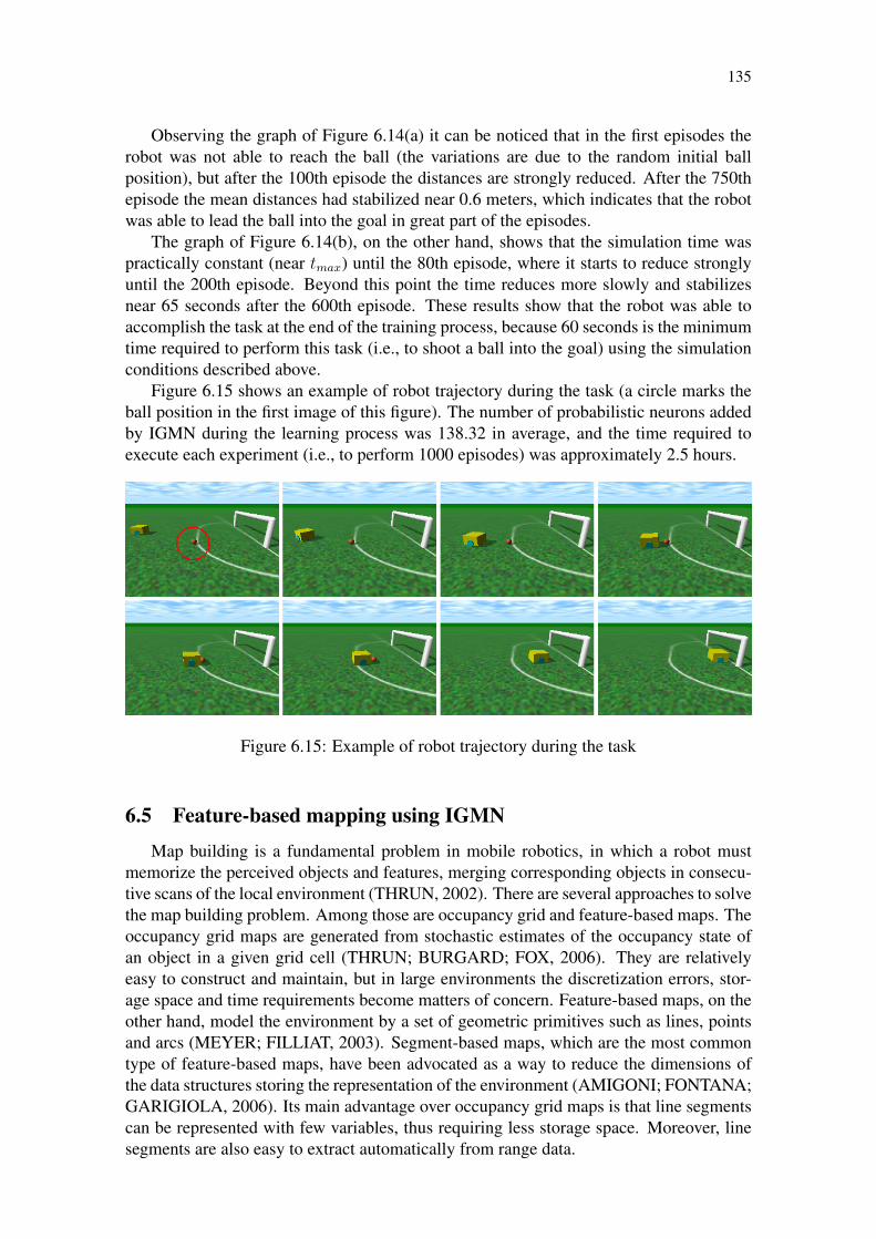
135
Observing the graph of Figure 6.14(a) it can be noticed that in the first episodes therobot was not able to reach the ball (the variations are due to the random initial ballposition), but after the 100th episode the distances are strongly reduced. After the 750thepisode the mean distances had stabilized near 0.6 meters, which indicates that the robotwas able to lead the ball into the goal in great part of the episodes.
The graph of Figure 6.14(b), on the other hand, shows that the simulation time waspractically constant (near tmax) until the 80th episode, where it starts to reduce stronglyuntil the 200th episode. Beyond this point the time reduces more slowly and stabilizesnear 65 seconds after the 600th episode. These results show that the robot was able toaccomplish the task at the end of the training process, because 60 seconds is the minimumtime required to perform this task (i.e., to shoot a ball into the goal) using the simulationconditions described above.
Figure 6.15 shows an example of robot trajectory during the task (a circle marks theball position in the first image of this figure). The number of probabilistic neurons addedby IGMN during the learning process was 138.32 in average, and the time required toexecute each experiment (i.e., to perform 1000 episodes) was approximately 2.5 hours.
Figure 6.15: Example of robot trajectory during the task
6.5 Feature-based mapping using IGMN
Map building is a fundamental problem in mobile robotics, in which a robot mustmemorize the perceived objects and features, merging corresponding objects in consecu-tive scans of the local environment (THRUN, 2002). There are several approaches to solvethe map building problem. Among those are occupancy grid and feature-based maps. Theoccupancy grid maps are generated from stochastic estimates of the occupancy state ofan object in a given grid cell (THRUN; BURGARD; FOX, 2006). They are relativelyeasy to construct and maintain, but in large environments the discretization errors, stor-age space and time requirements become matters of concern. Feature-based maps, on theother hand, model the environment by a set of geometric primitives such as lines, pointsand arcs (MEYER; FILLIAT, 2003). Segment-based maps, which are the most commontype of feature-based maps, have been advocated as a way to reduce the dimensions ofthe data structures storing the representation of the environment (AMIGONI; FONTANA;GARIGIOLA, 2006). Its main advantage over occupancy grid maps is that line segmentscan be represented with few variables, thus requiring less storage space. Moreover, linesegments are also easy to extract automatically from range data.

136
However, segment-based maps are not able to give closed and connected regions likeoccupancy grid maps because some objects do not provide line segments. Moreover, thenumber of extracted line segments is very high if the environment is irregular (not com-posed only by straight walls) and/or the range data is quite noisy. Another disadvantage ofsegment-based maps is the absence of probabilistic information in the generated map (al-though some researchers (GASÓS; MARTÍN, 1997; IP et al., 2002) have used fuzzy setsto deal with uncertainty in the mapping process). In fact, according to Thrun (2006), prob-abilistic approaches are typically more robust in face of sensor limitations, sensor noise,environment dynamics, and so on. Other localization and mapping techniques, such asparticle filters and potential fields, generally use grid maps to represent the environment,and therefore have the same restrictions pointed out above.
This section presents a new feature-based mapping algorithm, published in Heinenand Engel (2011; 2010c), which uses the IGMN probabilistic units to represent the fea-tures perceived in the environment. This kind of representation, which is inherently prob-abilistic, is more effective than segment-based maps because it has an arbitrary accuracy(it does not require discretization) and can even model objects that do not provide linesegments. Moreover, the proposed mapping algorithm does not require an exclusive kindof sensor (it can be used either with laser scanners or sonar sensors), requires low storagespace and is very fast, which allows it to be used in real time. The remainder of thissection is organized as follows: Subsection 6.5.1 describes some previous feature-basedmapping techniques; Subsection 6.5.2 describes how IGMN can be used to create feature-based maps; and Subsection 6.5.3 describes some experiments performed to evaluate theproposed mapping algorithm using sonar and laser range data.
6.5.1 Related work
In the last decade several feature-based mapping algorithms have been proposed tosolve the map building problem. In Zhang and Ghosh (2000) a segment-based mappingalgorithm is proposed that describes a line segment using the center of gravity of its pointsand the direction θ of its supporting line. This algorithm groups laser points in clusters,and for each cluster, a line segment is generated. In Lee et al. (2005) a feature basedmapping algorithm is presented which uses an association model to extract lines, pointsand arc features from sparse sonar data. In Puente et al. (2009) a mapping algorithm ispresented which uses a segmentation algorithm derived from computer vision techniquesto extract geometrical features from laser range data. In Latecki et al. (2004) a mappingalgorithm is proposed which represents the environment by polygonal curves (polylines).
In Amigoni, Fontana and Garigiola (2006) a method derived from the Lu and Milos’algorithm (LU; MILIOS, 1998) is presented for building segment-based maps that containa small number of line segments. In Amigoni, Gasparini and Gini (2006) an algorithmis proposed to build a global geometric map by integrating scans collected by laser rangescanners. This method, which considers scans as collections of line segments, workswithout any knowledge about the robot pose. In Luo et al. (2008) an indoor localizationmethod based on segment-based maps is proposed. It works in four steps: clustering scandata; feature extraction from laser data; line-based matching; and pose prediction. Butthis method assumes that the environment map already exists, i.e., it neither creates norupdates the map.
In Lorenzo et al. (2004) a method is proposed to solve the SLAM (Simultaneous Lo-calization and Map Building) problem based on segments extracted from local occupancymaps, in which line segments are categorized as new obstacle boundaries of a simultane-

137
ously built global segment-based map or as prolongations of previously extracted bound-aries. In Meyer-Delius and Burgard (2010) a point-based representation is described, inwhich the data points gathered by the robot are directly used as a non-parametric repre-sentation. To reduce the large memory requirements necessary to store all data points, anoff-line algorithm based on the fuzzy k-means is used to select the maximum-likelihoodsubsets of data points.
As described above, the main limitation of all these feature-based mapping techniquesis the absence of probabilistic information in the generated map. To avoid this limitation,Gasós et al. use fuzzy-segments to represent uncertainty in the feature positions (GASÓS;MARTÍN, 1997; GASÓS; ROSSETI, 1999). This model extracts segments from pointsprovided by sonar sensors, which are modeled on the map using fuzzy-sets. In the modelproposed by Ip et al. (2002), on the other hand, an adaptive fuzzy clustering algorithm isused to extract and classify line segments in order to build a complete map for an unknownenvironment.
Although these mapping techniques are able to create good representations in simpleenvironments composed by straight walls, most of them are not able to build the map inreal-time while the robot navigates in the environment (i.e., they are off-line solutions).The mapping algorithm proposed in this subsection, on the other hand, is able to buildenvironment representations in real time and incrementally. Moreover, it is inherentlyprobabilistic and does not assume a specific environment structure. The next subsectiondescribes how IGMN can be used in a feature-based mapping algorithm.
6.5.2 Incremental feature-based mapping using IGMN
This subsection describes a geometric-based mapping algorithm which uses the IGMNunits (also called mixture model components) to represent the features (objects, walls, etc)of the environment. Figure 6.16 shows the general architecture of the mapping algorithm.It consists mainly of two IGMN’s, the local model, which represents the local perceptionof the robot, and the global model, which represents the global environment map. EachIGMN has two cortical regions, N A and N B . The cortical region N A tackles the val-ues of the sensor readings and the cortical region N B receives the odometric informationprovided by the Pioneer 3-DX simulator.
Initially both models are empty. When a sensor reading arrives (which can be a laserscan or a sonar reading) it is transformed into object locations on a global coordinatesystem based on the robot position estimated by the dead reckoning system. These objectlocations are grouped in clusters using the IGMN algorithm, thus composing the localmodel. When a specified number N of sensor readings arrives (e.g., 10 laser scans or 100sonar readings), the local model is matched against the global model. If the global modelis still empty, all local units are added to it and deleted from the local model. Otherwise therobot pose is adjusted to minimize the differences between the local and global modelsusing the component matching process described in the next subsection. Both IGMNmodels are then merged into the global model and the local model is emptied. When anew sensor reading arrives, all these steps are repeated, and so the global model is updatedat each N readings.
All this process occurs in real time at normal sensor arriving speeds (e.g., one laserscan at each 100 milliseconds) even with more than 500 Gaussian units in the IGMNmodels. In fact, the prototype was able to perform all these operations (including thematching and merging processes) in less than 30 milliseconds on the same typical com-puter described before. In relation to memory requirements, the proposed mapping algo-

138
Figure 6.16: General architecture of the proposed mapping algorithm
rithm is very parsimonious, requiring just eight floating point numbers to store each two-dimensional Gaussian distribution (D2 +D + 2 floating-point variables, where D = 2 isthe dimension of the map).
6.5.2.1 Component matching
In the proposed mapping algorithm, the robot maintains knowledge about its poseusing data coming from odometry, which is an unreliable source of information (THRUN;BURGARD; FOX, 2006). In order to refine the estimated robot poses, the local model,which represents the robot current view, is matched against the global model, and thedifferences are used to adjust the estimated pose of the robot and the local units.
The matching process used here is inspired in the Lu and Milos’ algorithm (LU; MIL-IOS, 1998) and works in the following way. Initially, all spurious components (i.e., thoseunits which represent few data points and/or noise) of the local model are excluded. Aunit j is considered spurious if its density is lower than a minimum value ρmin. The den-sity ρj of a cluster j is computed using the following equation adapted from Gath andGeva (1989):
ρj =spj
(2π)D/2√|Cj|
(6.5)
where D is the dimensionality of the data points (2 for a two-dimensional map), C is thevariance/covariance matrix of the j unit, and spj is the accumulator of the a posterioriprobabilities.
A low cluster density ρj indicates that the cluster j represents few data points com-pared to its size, which in our case may represent that j was generated by few and sparse(possibly noisy) sensor readings. Moreover, if a cluster is almost parallel to the sensorbeam, i.e., the angles of the cluster main axis (computed using its eigenvectors) and thesensor beam (the line segment linking the sensor to the center of the cluster) differ by lessthan a user-specified parameter αmin, this cluster is also considered spurious because thereadings are not reliable.

139
The next step in the proposed algorithm is to find equivalent components in bothmodels, i.e., those clusters corresponding to the same environment features. Two clustersare considered equivalent if: (i) the difference between the cluster orientations is lowerthan a user-specified parameter αmax; (ii) the Mahalanobis distance between the centerµ of each unit (computed using the covariance matrix C of the global model) is lowerthan a user-specified parameter ηmax. Those global units invisible from the current robotviewpoint (i.e., the orientation of the segment(s) linking the sensor(s) to the cluster is outof range) are not considered here. The output of this process is a list containing the pairsof equivalent Gaussian components in both models.
The new robot pose is computed using the Powell’s direction set method (POWELL,1964; PRESS et al., 1992), in order to minimize the discrepancies Elg among the equiva-lent global g and local l units, i.e.:
Elg =1
M
M∑i=1
(αgi − αli)2 +DM (µgi, µli) (6.6)
where M is the number of matching pairs and DM (·) is the Mahalanobis distance com-puted using the covariance matrix of the global unit Cg. The robot pose derived from theodometry is used as an initial guess in the minimization process. In general the Powell’smethod converges fast if this initial guess is reasonable, which is the case here becauseodometric information is reliable in short distances.
6.5.2.2 Component merging
In this procedure, the local components which are not spurious are inserted into theglobal model, thus expanding it to reflect the new perceived environment features. Thisinsertion procedure occurs in two different steps. Initially the global clusters which haveequivalents in the local model (i.e., those that are present in the list of matching pairsdescribed previously) are updated using the following equations (DECLERCQ; PIATER,2008):
µ∗g =spgµg + splµlspg + spl
(6.7)
C∗g =spgCg + splCl
spg + spl+spgµgµg
T + splµlµlT
spg + spl− µ∗gµ
∗gT (6.8)
sp∗g = spg + spl (6.9)where µg is the old mean vector of the global unit g and µ∗g is the new mean vectorcomputed by (6.7) at time t. The local clusters that have no counterparts in the globalmodel (i.e., those that represent new environment features) are simply inserted into theglobal model without modification. This also occurs in the beginning of the mappingprocess (when the global model is empty).
After merging, all local units are removed from the local model and the prior proba-bilities p of all global units are updated by:
p∗g =spg∑Mj=1 spj
(6.10)
where M is the current number of global units. This global model represents the en-vironment using occupancy probabilities, i.e., for each (x, y) coordinate it is possibleto compute the probability that an obstacle (e.g., wall) is present in that location. Nextsubsection describes several experiments performed to evaluate the performance of theproposed mapping algorithm in robot mapping tasks.

140
6.5.3 Experiments
This subsection describes some experiments performed to evaluate the proposed map-ping algorithm using two kinds of sensory information: (i) data provided by a simulatedlaser scanner; and (ii) data provided by sonar sensors. The robot used in these experimentsis a Pioneer 3-DX, shown in Figure 6.3 above. This robot has a Sick LMS-200 laser scan-ner installed on it, which in ideal conditions is capable of measuring out to 80m over a180arc. Figure 6.17 shows the real environment used in the simulation. It is composedby two long corridors of 2.3× 30 meters linked by two short corridors of 2.3× 10 meters,as shown in the schematic map presented in Figure 6.17(c). This environment has severalirregularities (e.g. doors, saliences and printers) which difficult the mapping process.
(a) Long corridor (b) Short corridor
(c) Schematic map of the environment
Figure 6.17: Environment used in the feature-based mapping experiments
The configuration parameters used in all experiments are: δ = 0.1; ρmin = 10−5;αmin = 10; αmax = 10 and ηmax = 2 (the proposed algorithm is not sensible tothese parameters). The only configuration parameter that needs to be adjusted to eachexperiment is the τnov ∈ (0, 1] parameter, which in this case defines the granularity ofthe model, i.e., small values (<< 0.01) produce few larger clusters, and larger values(≥ 0.01) produce several little clusters. As in Section 6.1, here we decided to use theτnov parameter instead of εmax because in these experiments the goal is to find naturalgroupings (i.e., clusters) rather than function approximation. In the next subsections wedescribe experiments performed using data provided by a simulated laser scanner and asonar range data.

141
6.5.3.1 Experiments using simulated laser scanner data
This subsection describes two experiments performed using sensor data provided bya simulated laser scanner that is equivalent to the Sick LMS-200 installed on the realPioneer 3-DX robot. In these experiments, the robot was manually controlled to performone loop in the simulated environment shown in Figure 6.17(c). A complete laser scan isreceived at each 100 milliseconds, and the mapping process is performed at each second(i.e., using 10 complete scans). The first experiment was conducted using τnov = 10−8,and this small value produced 9 large clusters, as can be seen in Figure 6.18.
Figure 6.18: Gaussian distributions generated using laser data (τnov = 10−8)
Figure 6.19: Occupancy probabilities of Figure 6.18 model
In this figure, each cluster is represented by an ellipse whose width is equivalent to aMahalanobis distance of two. The occupancy probabilities of this map are graphicallyshown in Figure 6.19, where darker regions represent higher occupancy probabilities(close to 1) and lighter regions correspond to probabilities close to 0. It is importantto highlight that the proposed mapping algorithm does not have any random initializationand/or decision, and thus the obtained results are always identical for the same datasetand configuration parameters.
The next experiment was performed using the same conditions described above, butusing a larger τnov = 10−2 value which makes the system more sensible to small variationsin the laser data. The results obtained in this experiment are shown in Figures 6.20 and6.21. It can be noticed from Figure 6.20 that much more clusters were generated in thisexperiment (76 Gaussian components were generated). Nevertheless, these clusters fitvery well the environment features, existing almost one cluster for each feature (doorsentrances, saliences in the walls, etc.). Moreover, each wall is modeled by a thin, longcluster which closely represents the center of the wall.

142
Figure 6.20: Gaussian distributions generated using laser data (τnov = 10−2)
Figure 6.21: Occupancy probabilities of Figure 6.20 model
These experiments show that the proposed mapping algorithm is able to create usefulrepresentations of the environment, and these representations can be coarse (Figure 6.18)or fine (Figure 6.20) depending on the τnov configuration value. Although these experi-ments were performed using high quality simulated laser range data, the proposed map-ping algorithm is not restricted to this kind of sensory data. In the next subsection wedescribe an experiment performed using this same environment, but with data providedby real sonar sensors, which are less accurate and noisier than laser scanners.
6.5.3.2 Experiments using real sonar data
In these experiments, the proposed mapping algorithm is evaluated using data pro-vided by the sonar sensor array of the real Pioneer 3-DX robot. The time interval of eachscan is 100 milliseconds, and the local model is generated using 100 complete scans (i.e.,at each 10 seconds). Figure 6.22 shows the global model generated after one loop in theenvironment, and Figure 6.23 illustrates the occupancy probabilities of this map, wheredarker regions represents higher probabilities. The configuration parameters used in thisexperiment are the same of the previous one (i.e., τnov = 10−2).
We can notice that even with many noise sources present in the environment, theproposed mapping algorithm was able to create a reasonable map of the environmentusing these very noisy sensory data. The results obtained in Figure 6.22 show that theproposed mapping algorithm does not require just laser scanner sensors, but of course thequality of the maps is superior when high quality sensor data is used.
Although in this experiment more Gaussian distributions were generated (216), this isyet a small number compared to the number of cells necessary to map this environment

143
Figure 6.22: Distributions generated using sonar sensors (τnov = 10−2)
Figure 6.23: Occupancy probabilities of Figure 6.22 model
using grid-based mapping techniques. In fact, to obtain a similar performance using aoccupancy grid maps it would be necessary a large number of cells. To demonstratethis, Figure 6.24 shows a grid map generated using the same real data that generated themap presented in Figure 6.23, i.e., the real sensor readings adjusted using the matchingtechnique proposed in this paper. Each cell in Figure 6.24 represent an area of 20 × 20centimeters, and 200 × 80 = 16000 were necessary to represent this map. It can benoticed in Figure 6.24 that even using 16000 cells the map resolution is inferior thanthat presented in Figure 6.23. Moreover, the number and size of the grid cells must bepreviously informed and kept fixed.
Figure 6.24: Grid map generated using the same data of Figure 6.24

144
A interesting characteristic of the mapping algorithm proposed here is that the occu-pancy probabilities of the unvisited regions are near zero, whilst using a grid-based mapthese regions will have occupancy probabilities near to 50%. This characteristic is a natu-ral consequence of representing just the occupied regions in the environment map, and isalso shared by other kinds of feature-based maps such as segment-based maps. However,this characteristic is very useful because it encourage the exploration of unvisited regions.In fact, if a region has an occupancy probability near zero the robot will try to navigatethrough this region, and then it finds out the actual structure of this region and the map willbe improved and/or expanded. Hence, this characteristic allows an exploration strategythat follows the Autotelic principle (STEELS, 2004), which states that an agent must beself-motivated for learning and improving its skills. Moreover, this strategy is not basedon ad-hoc choices nor configuration parameters.
6.5.3.3 Complex simulated environments
The next experiment was performed using the Pioneer 3-DX simulator software AR-COS (Advanced Robot Control & Operations Software) and the “AMROffice.map” envi-ronment (Figure 6.25), a complex map generated using real data and distributed with therobot simulator. The time interval of each scan is 100 milliseconds, and the local mixturemodel is generated using 100 complete scans.
Figure 6.25: AMROffice environment
Figure 6.26(a) shows the map generated in the first experiment. The number of Gaus-sian mixtures generated in the global model was 364, which is a small value comparedto the number of cells necessary to map this environment using grid-based mapping tech-niques. The occupancy probabilities of this map are graphically shown in Figure 6.26(b),where darker regions represent higher occupancy probabilities (close to 1) and lighterregions correspond to probabilities close to 0.

145
(a) Generated map (b) Occupancy probabilities
Figure 6.26: Results obtained in the AMROffice environment
The proposed model has also obtained good results in the irregular environment pre-sented in Figure 6.9, as shows Figure 6.27. We can notice in Figure 6.27 that the Gaussiandistributions are perfectly aligned with the external wall of the environment. In this figurewe have represented the map using rectangles rather than ellipses to better visualize thealignment of the Gaussian units with the modeled structures. Moreover, we can see in
Figure 6.27: Map generated in an irregular environment
Figure 6.28, which shows the occupancy probabilities by ellipses, that the internal objectswere modeled using larger distributions. This occurs because the perception of the robotis occluded in some parts of the environment, which prevents the mapping algorithm toaccurately represent the internal faces of some objects (the trajectory followed by the

146
robot is that shown by the solid gray line in Figure 6.9). Nevertheless, we can notice thatthe generated map is quite good, because it represents the irregular environment in a veryparsimonious and effective way.
Figure 6.28: Occupancy probabilities of the irregular environment
This chapter has presented several experiments in which IGMN was used in real timerobotic applications and related tasks. Through these experiments we can notice thatIGMN is very suitable for those tasks, and its efficient learning algorithm and representa-tional power can expand the set of potential applications of neural networks. Next sectionpresents the final conclusions of this thesis.

147
7 CONCLUSION AND FUTURE WORK
This monograph has presented IGMN, a new connectionist approach for incremen-tal function approximation and on-line prediction, that is the main contribution of thisthesis. IGMN is inspired on recent theories about the brain, specially the Memory-Pre-diction Framework (MPF) (HAWKINS, 2005) and the constructivist artificial intelligence(DRESCHER, 1991), which endows it with some unique features that are not present inother ANN models such as MLP, RBF and GRNN. More specifically in IGMN we don’tuse the words input and output to represent the data features of a training sample such asz = a,b, for instance. Instead, we consider that the data vectors a and b are differentsensory and/or motor modalities with distinct domains, and one modality (e.g. a) can beused to estimate another (e.g. b). Moreover, IGMN is based on strong statistical princi-ples (Gaussian mixture models) and asymptotically converges to the optimal regressionsurface as more training data arrive.
To validate the proposed model, several experiments were performed using syntheticdata (e.g., sinusoid datasets) and these experiments have demonstrated that: (i) IGMNlearns incrementally using a single scan over the training data; (ii) It does not require tofine tune its configuration parameters (in fact just a single and easy to adjust configurationparameter must be set); (iii) IGMN is relatively robust to the order of presentation ofdata; (iv) the proposed model can provide the confidence levels of its estimates; and (v)the IGMN performance is comparable to those of other ANN models (e.g., MLP, RBF,GRNN) but without requiring that the training data set be complete and available at thebeginning of the learning process.
IGMN was also tested in practical applications such as: (i) the identification of anonlinear plant; (ii) time series prediction; (iii) concept formation; (iv) reinforcementlearning; and (iv) robotic mapping and control, and these experiments have shown thatIGMN can be used successfully in applications that require incremental learning and/orreal time performance. More specifically, the performed experiments have demonstratedthat IGMN has the following advantages over the existing connectionist approaches:
The IGMN learning algorithm is very aggressive. As said before, IGMN learns in-crementally using a single scan over the training data, i.e., each training pattern can beimmediately used and discarded. Moreover, IGMN can produce reasonable estimatesbased on few training data, and these estimates are improved as new training data arrive.
The learning process can proceed perpetually. Unlike other ANN models, IGMN doesnot require separate phases for learning and recalling, i.e., the learning process can pro-ceed perpetually without suffering from catastrophic interference. Hence, the proposedmodel can always improve its performance as new data arrive and consequently the neuralnetwork can adapt itself to changes in the environment.
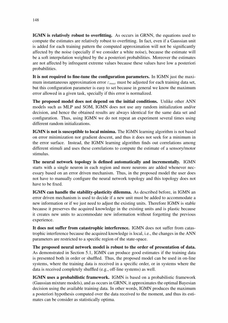
148
IGMN is relatively robust to overfitting. As occurs in GRNN, the equations used tocompute the estimates are relatively robust to overfitting. In fact, even if a Gaussian unitis added for each training pattern the computed approximation will not be significantlyaffected by the noise (specially if we consider a white noise), because the estimate willbe a soft interpolation weighted by the a posteriori probabilities. Moreover the estimatesare not affected by infrequent extreme values because these values have low a posterioriprobabilities.
It is not required to fine-tune the configuration parameters. In IGMN just the maxi-mum instantaneous approximation error εmax must be adjusted for each training data set,but this configuration parameter is easy to set because in general we know the maximumerror allowed in a given task, specially if this error is normalized.
The proposed model does not depend on the initial conditions. Unlike other ANNmodels such as MLP and SOM, IGMN does not use any random initialization and/ordecision, and hence the obtained results are always identical for the same data set andconfiguration. Thus, using IGMN we do not repeat an experiment several times usingdifferent random initializations.
IGMN is not is susceptible to local minima. The IGMN learning algorithm is not basedon error minimization nor gradient descent, and thus it does not seek for a minimum inthe error surface. Instead, the IGMN learning algorithm finds out correlations amongdifferent stimuli and uses these correlations to compute the estimate of a sensory/motorstimulus.
The neural network topology is defined automatically and incrementally. IGMNstarts with a single neuron in each region and more neurons are added whenever nec-essary based on an error driven mechanism. Thus, in the proposed model the user doesnot have to manually configure the neural network topology and this topology does nothave to be fixed.
IGMN can handle the stability-plasticity dilemma. As described before, in IGMN anerror driven mechanism is used to decide if a new unit must be added to accommodate anew information or if we just need to adjust the existing units. Therefore IGMN is stablebecause it preserves the acquired knowledge in the existing units and is plastic becauseit creates new units to accommodate new information without forgetting the previousexperience.
It does not suffer from catastrophic interference. IGMN does not suffer from catas-trophic interference because the acquired knowledge is local, i.e., the changes in the ANNparameters are restricted to a specific region of the state-space.
The proposed neural network model is robust to the order of presentation of data.As demonstrated in Section 5.1, IGMN can produce good estimates if the training datais presented both in order or shuffled. Thus, the proposed model can be used in on-linesystems, where the training data is received in a specific order, or in systems where thedata is received completely shuffled (e.g., off-line systems) as well.
IGMN uses a probabilistic framework. IGMN is based on a probabilistic framework(Gaussian mixture models), and as occurs in GRNN, it approximates the optimal Bayesiandecision using the available training data. In other words, IGMN produces the maximuma posteriori hypothesis computed over the data received to the moment, and thus its esti-mates can be consider as statistically optima.
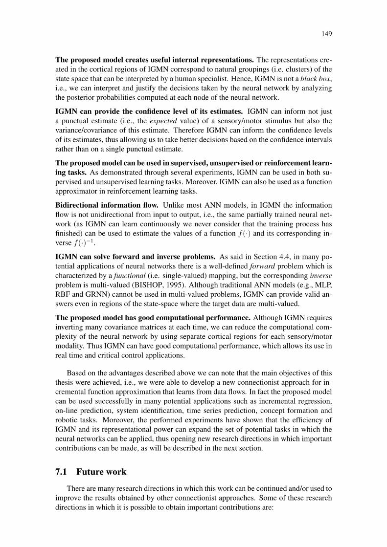
149
The proposed model creates useful internal representations. The representations cre-ated in the cortical regions of IGMN correspond to natural groupings (i.e. clusters) of thestate space that can be interpreted by a human specialist. Hence, IGMN is not a black box,i.e., we can interpret and justify the decisions taken by the neural network by analyzingthe posterior probabilities computed at each node of the neural network.
IGMN can provide the confidence level of its estimates. IGMN can inform not justa punctual estimate (i.e., the expected value) of a sensory/motor stimulus but also thevariance/covariance of this estimate. Therefore IGMN can inform the confidence levelsof its estimates, thus allowing us to take better decisions based on the confidence intervalsrather than on a single punctual estimate.
The proposed model can be used in supervised, unsupervised or reinforcement learn-ing tasks. As demonstrated through several experiments, IGMN can be used in both su-pervised and unsupervised learning tasks. Moreover, IGMN can also be used as a functionapproximator in reinforcement learning tasks.
Bidirectional information flow. Unlike most ANN models, in IGMN the informationflow is not unidirectional from input to output, i.e., the same partially trained neural net-work (as IGMN can learn continuously we never consider that the training process hasfinished) can be used to estimate the values of a function f(·) and its corresponding in-verse f(·)−1.
IGMN can solve forward and inverse problems. As said in Section 4.4, in many po-tential applications of neural networks there is a well-defined forward problem which ischaracterized by a functional (i.e. single-valued) mapping, but the corresponding inverseproblem is multi-valued (BISHOP, 1995). Although traditional ANN models (e.g., MLP,RBF and GRNN) cannot be used in multi-valued problems, IGMN can provide valid an-swers even in regions of the state-space where the target data are multi-valued.
The proposed model has good computational performance. Although IGMN requiresinverting many covariance matrices at each time, we can reduce the computational com-plexity of the neural network by using separate cortical regions for each sensory/motormodality. Thus IGMN can have good computational performance, which allows its use inreal time and critical control applications.
Based on the advantages described above we can note that the main objectives of thisthesis were achieved, i.e., we were able to develop a new connectionist approach for in-cremental function approximation that learns from data flows. In fact the proposed modelcan be used successfully in many potential applications such as incremental regression,on-line prediction, system identification, time series prediction, concept formation androbotic tasks. Moreover, the performed experiments have shown that the efficiency ofIGMN and its representational power can expand the set of potential tasks in which theneural networks can be applied, thus opening new research directions in which importantcontributions can be made, as will be described in the next section.
7.1 Future work
There are many research directions in which this work can be continued and/or used toimprove the results obtained by other connectionist approaches. Some of these researchdirections in which it is possible to obtain important contributions are:

150
• Hierarchic representation: The proposed model can be expanded to create hierar-chies of Gaussian units in a similar way to those proposed in the memory predictionframework (MPF) (HAWKINS, 2005; HAWKINS; DILEEP, 2006; PINTO, 2009);• Hierarchical reinforcement learning: The RL algorithm proposed in Section 6.4
can be modified into a hierarchical RL algorithm (BARTO; MAHADEVAN, 2003;MOERMAN, 2009), thus improving the learning performance by dividing the com-plete state space in subregions;• Time series prediction: IGMN can be used to predict more complex, chaotic and
cyclic time series;• The inverse kinematics problem: to use IGMN for computing the inverse kinematics
of more complex robotic arms composed by many joints and with six degrees offreedom;• Simultaneous localization and mapping (SLAM): The feature-based mapping algo-
rithm presented in Section 6.5 can be expanded to a SLAM solution by using IGMNto predict the robot’s position as it navigates through the environment;• Multi-hypothesis tracking: IGMN can implement a global localization mechanism
(FILLIAT; MEYER, 2003) that allows the robot to recover its position even fromthe kidnapped robot problem (THRUN; BURGARD; FOX, 2006).• Autotelic exploration: to implement an exploration algorithm based on the Au-
totelic principle (STEELS, 2004) that self-motivates the robot to explore new re-gions and/or to develop new skills;• Attentional mode neural network: IGMN can be combined with the attentional
mode neural network (AMNN) (ENGEL, 1996) in order to improve both modelsand to obtain more stable results in control tasks (currently AMNN learns fasterthan RL (SUTTON; BARTO, 1998), but it suffers from catastrophic interference);• Classification: although in this thesis we are interested just in regression, IGMN
can be easily adapted to be used in supervised classification tasks.
Hence we can notice that there are many improvements that can be made over thework presented in this thesis, and hence we can affirm that IGMN is a very useful machinelearning tool that expands the horizon of tasks in which the artificial neural networks canbe used successfully and efficiently.

151
REFERENCES
AMIGONI, F.; FONTANA, G.; GARIGIOLA, F. Distributed Autonomous RoboticSystems (DARS). Berlin, Germany: Springer-Verlag, 2006. v.7, p.11–20.
AMIGONI, F.; GASPARINI, S.; GINI, M. Building Segment-Based Maps Without PoseInformation. Proceedings of the IEEE, Los Alamitos, CA, USA, v.94, n.7, p.1340–1359,July 2006.
ARANDJELOVIC, O.; CIPOLLA, R. Incremental Learning of Temporally-CoherentGaussian Mixture Models. In: BRITISH MACHINE VISION CONFERENCE (BMVC),16., Oxford, UK. Proceedings. . . British Machine Vision Association (BMVA), 2005.p.759–768.
ASADA, M. et al. Purposive Behavior Acquisition for a Real Robot by Vision-BasedReinforcement Learning. Machine Learning, Boston, MA, USA, v.23, p.279–303, 1996.
ASADA, M. et al. A Humanoid Approaches to the Goal - Reinforcement Learning Basedon Rhythmic Walking Parameters. In: INTERNATIONAL ROBOCUP SYMPOSIUM,7., Padua, Italy. Proceedings. . . Springer-Verlag, 2003. p.344–354. (Lecture Notes inComputer Science, v.3020).
ASHBY, W. R. An Introduction to Cybernetics. London, UK: Chapman & Hall, 1956.308p.
ATTIAS, H. A Variational Bayesian Framework for Graphical Models. Neural Informa-tion Processing Systems (NIPS), Cambridge, MA, USA, v.12, p.209–215, 2000.
BAKKER, B. et al. A Robot that Reinforcement-Learns to Identify and Memorize Impor-tant Previous Observations. In: IEEE/RSJ INTERNATIONAL CONFERENCE ON IN-TELLIGENT ROBOTS AND SYSTEMS (IROS), Las Vegas, NV, USA. Proceedings. . .IEEE Press, 2003. v.1, p.430–435.
BAKKER, B.; LINÅKER, F.; SCHMIDHUBER, J. Reinforcement Learning in PartiallyObservable Mobile Robot Domains Using Unsupervised Event Extraction. In: IEEE/RSJINTERNATIONAL CONFERENCE ON INTELLIGENT ROBOTS AND SYSTEMS(IROS), EPFL, Lausanne, Switzerland. Proceedings. . . IEEE Press, 2002. v.1, p.938–943.
BARRON, A. R.; BARRON, R. L. Statistical Learning Networks: A unifying view. In:SYMPOSIUM ON THE INTERFACE: STATISTICS AND COMPUTING SCIENCE,Virginia, USA. Proceedings. . . Reston, 1988.

152
BARTO, A. G.; MAHADEVAN, S. Recent Advances in Hierarchical ReinforcementLearning. Discrete Event Dynamic Systems, Netherlands, v.13, n.4, p.341–379, 2003.
BASSO, E. W.; ENGEL, P. M. Reinforcement Learning in Non-Stationary ContinuousTime and Space Scenarios. In: ARTIFICIAL INTELLIGENCE NATIONAL MEETING(ENIA), 7., Bento Gonçalves, RS, Brazil. Proceedings. . . SBC Editora, 2009.
BASTOS, E. N. F. Uma Rede Neural Auto-Organizável Construtiva para Apren-dizado Perpétuo de Padrões Espaço-Temporais. 2007. Master’s Thesis — UniveridadeFederal do Rio Grande do Sul (UFRGS), Porto Alegre, RS, Brazil. Text in Portuguese.
BEKEY, G. A. Autonomous Robots: from biological inspiration to implementation andcontrol. Cambridge, MA, USA: The MIT Press, 2005. 577p.
BERGER, J. O. Statistical Decision Theory and Bayesian Analysis. 2.ed. New York,NY, USA: Springer-Verlag, 1980. 627p.
BERTHOLD, M. R.; DIAMOND, J. Constructive Training of Probabilistic Neural Net-works. Neurocomputing, New York, NY, USA, v.19, p.167–183, 1998.
BHATTACHARYYA, N. et al. Incremental PNN Classifier for a Versatile ElectronicNose. In: INTERNATIONAL CONFERENCE ON SENSING TECHNOLOGY, 3.,Tainan, Taiwan. Proceedings. . . IEEE Press, 2008. p.242–247.
BISHOP, C. M. Neural Networks for Pattern Recognition. New York, USA: OxfordUniversity Press, 1995. 482p.
BLEI, D. M.; JORDAN, M. I. Variational Inference for Dirichlet Process Mixtures. Jour-nal of Bayesian Analysis, Columbus, OH, USA, v.1, n.1, p.121–144, 2005.
BOX, G. E. P.; JENKINS, G. M.; REINSEL, G. C. Time Series Analysis: forecastingand control. 3.ed. San Francisco, CA, USA: Holden Day, 1976. 575p.
BRENT, R. P. Algorithms for Minimization without Derivatives. Englewood Cliffs,NJ, USA: Prentice-Hall, 1973.
BURFOOT, D.; LUNGARELLA, M.; KUNIYOSHI, Y. Toward a Theory of Embod-ied Statistical Learning. In: INTERNATIONAL CONFERENCE ON SIMULATION OFADAPTIVE BEHAVIOR (SAB 2008), 10., Berlin, Heidelberg. Proceedings. . . Springer-Verlag, 2008. p.270–279. (Lecture Notes in Artificial Intelligence, v.5040).
CACOULLOS, T. Estimation of a Multivariate Density. Annals of the Institute of Sta-tistical Mathematics, Tokyo, Japan, v.18, p.179–189, Sept. 1966.
CAMARGO, S. S. Um Modelo Neural de Aprimoramento Progressivo para Reduçãode Dimensionalidade. 2010. Ph.D. thesis — Univeridade Federal do Rio Grande do Sul(UFRGS), Porto Alegre, RS, Brazil. Text in Portuguese.
CAMARGO, S. S.; ENGEL, P. M. Time Series Prediction with Focused Time LaggedFeed-Forward Networks. In: INTERNATIONAL SYMPOSIUM ON FORECASTING(ISF), 25., San Antonio, TX, USA. Proceedings. . . International Institute of Forecasting,2005. p.123.

153
CAPPÉ, O.; MOULINES, E. Online EM Algorithm for Latent Data Models. Journal ofthe Royal Statistical Society, London, UK, Sept. 2008.
CARPENTER, G. A. et al. Fuzzy ARTMAP: A neural network architecture for incremen-tal supervised learning of analog multidimensional maps. IEEE Transactions on NeuralNetworks, Los Alamitos, CA, USA, v.3, n.5, p.698–713, Sept. 1992.
CARPENTER, G. A.; GROSSBERG, S. A Massively Parallel Architecture for a Self-Organizing Neural Pattern Recognition Machine. Computer Vision, Graphics and Im-age Processing, New York, NY, USA, v.37, p.54–115, 1987.
CARPENTER, G. A.; GROSSBERG, S. Adaptive Resonance Theory. In: ARBIB,M. A. (Ed.). The Handbook of Brain Theory and Neural Networks. 2.ed. Cambridge,MA, USA: The MIT Press, 2003. p.87–90.
CARPENTER, G. A.; GROSSBERG, S.; REYNOLDS, J. ARTMAP: supervised real-time learning and classification of nonstationary data by a self-organizing neural network.Neural Networks, Oxford, UK, v.4, p.565–588, 1991.
CARPENTER, G. A.; GROSSBERG, S.; ROSEN, D. B. Fuzzy ART: fast stable learn-ing and categorization of analog patterns by an adaptive resonance system. Boston, MA,USA: Boston University, 1991. Neural Networks – Techincal Report. (CAS/CNS-TR-91-015).
CHANG, R. K. Y.; LOO, C. K.; RAO, M. V. C. Enhanced Probabilistic Neural Networkwith Data Imputation Capabilities for Machine-Fault Classification. Neural Computingand Applications, London, UK, v.18, p.791–800, 2009.
CHAPUT, H. H. The Constructivist Learning Architecture: A model of cognitive de-velopment for robust autonomous robots. 2004. Ph.D. Thesis — University of Texas,Austin, TX, USA.
CHEN, S.; COWAN, C. F. N.; GRANT, P. M. Orthogonal Least Squares Learning Al-gorithm for Radial Basis Function Networks. IEEE Transactions on Neural Networks,Los Alamitos, CA, USA, v.2, p.302–309, Mar. 1991.
CHOI, S. P. M.; YAN-YEUNG, D.; ZHANG, N. L. Hidden-Mode Markov Decision Pro-cesses for Nonstationary Sequential Decision Making. Sequence Learning – Paradigms,Algorithms, and Applications, London, UK, p.264–287, 2001.
COLLINS, M. The EM Algorithm. Burnaby, BC, Canada: School of Computing Sci-ence, Simon Fraser University (SFU), 1997. Technical Report. (CMPT-825).
COPPERSMITH DON; WINOGRAD, S. Matrix Multiplication Via Arithmetic Progres-sions. SIAM News, Philadelphia, PA, USA, v.9, n.3, p.251–280, 1990.
COX, D. R.; HINKLEY, D. V. Theoretical statistics. London, UK: Chapman and Hall,1974. 511p.
CRICK, F. The Astonishing Hypothesis: the scientific search for the soul. London, UK:Simon & Schuster, 1994. 317p.

154
CSÁJI, B. C. Approximation with Artificial Neural Networks. 2001. M.Sc. Thesis —Eindhoven University of Technology, The Netherlands.
CWIK, J.; KORONACKI, J. Probability Density Estimation using a Gaussian ClusteringAlgorithm. Neural Computing and Applications, London, UK, v.4, p.149–160, 1996.
DAMASIO, A. R. Descartes’ Error: emotion, reason, and the human brain. New York,NY, USA: HarperCollins, 1994. 316p.
DECLERCQ, A.; PIATER, J. H. Online Learning of Gaussian Mixture Models: A two-level approach. In: THIRD INTERNATIONAL CONFERENCE ON COMPUTER VI-SION THEORY AND APPLICATIONS (VISAPP), Funchal, Madeira, Portugal. Pro-ceedings. . . Springer-Verlag, 2008. v.1.
DELGOSHA, F.; MENHAJ, M. B. Fuzzy Probabilistic Neural Networks: A practicalapproach to the implementation of baysian classifier. In: REUSCH, B. (Ed.). Computa-tional Intelligence: theory and applications. Berlin, Germany: Springer Berlin / Heidel-berg, 2001. p.76–85. (Lecture Notes in Computer Science, v.2206).
DEMPSTER, A. P.; LAIRD, N. M.; RUBIN, D. B. Maximum Likelihood from Incom-plete Data Via the EM Algorithm. Journal of the Royal Statistical Society, London,UK, v.39, n.1, p.1–38, 1977.
DENNETT, D. C. Kinds of Minds: towards an understanding of consciousness. NewYork, NY, USA: Basic Books, 1996. 192p.
DOMINGOS, P.; HULTEN, G. H. A General Framework for Mining Massive DataStreams. Journal of Computational and Graphical Statistics, Alexandria, VA, USA,v.12, 2003.
DOYA, K. Temporal Difference Learning in Continuous Time and Space. Advances inNeural Information Processing Systems, Cambridge, MA, USA, v.8, p.1073–1079,1996.
DOYA, K. Reinforcement Learning in Continuous Time and Space. Neural Computa-tion, Cambridge, MA, USA, v.12, n.1, p.219–245, 2000.
DRESCHER, G. L. Made-up Minds: A constructivist approach to artificial intelligence.Cambridge, MA, USA: The MIT Press, 1991. 220p.
DUDEK, G.; JENKIN, M. Computational Principles of Mobile Robotics. Cambridge,UK: Cambridge University Press, 2000.
EDELMAN, G. M. Group Selection and Phasic Reentrant Signalling: A theory of higherbrain function. In: EDELMAN, G. M.; MOUNTCASTLE, V. B. (Ed.). The MindfulBrain: cortical organization and the group-selective theory of higher brain function. Cam-bridge, MA, USA: The MIT Press, 1978. p.51–100.
EDELMAN, G. M. Neural Darwinism: the theory of neuronal group selection. NewYork, NY, USA: Basic Books, 1987. 371p.
ELMAN, J. L. Finding Structure in Time. Cognitive Science, Hoboken, NJ, USA, v.14,n.2, p.179–211, 1990.

155
ENGEL, P. M. Attentional Mode Neural Network: A new approach for real-timeself-learning. In: IEEE INTERNATIONAL SYMPOSIUM ON CIRCUITS AND SYS-TEMS(ISCAS’96). Proceedings. . . IEEE Press, 1996. p.45–48.
ENGEL, P. M. INBC: An incremental algorithm for dataflow segmentation based on aprobabilistic approach. Porto Alegre, RS, Brazil: UFRGS, 2009. Technical Report. (RP-360).
ENGEL, P. M.; HEINEN, M. R. Concept Formation using Incremental Gaussian Mix-ture Models. In: IBEROAMERICAN CONGRESS ON PATTERN RECOGNITION(CIARP), 15., São Paulo, SP, Brazil. Proceedings. . . Springer-Verlag, 2010. p.128–135.(Lecture Notes in Computer Science, v.6419).
ENGEL, P. M.; HEINEN, M. R. Incremental Learning of Multivariate Gaussian MixtureModels. In: BRAZILIAN SYMPOSIUM ON AI (SBIA): ADVANCES IN ARTIFICIALINTELLIGENCE, 20., São Bernardo do Campo, SP, Brazil. Proceedings. . . Springer-Verlag, 2010. p.82–91. (Lecture Notes in Artificial Intelligence, v.6404).
EVES, H. Foundations and Fundamental Concepts of Mathematics. 3.ed. Mineola,NY, USA: Dover Publications, Inc., 1990.
FAHLMAN, S. E.; LEBIERE, C. The Cascade-Correlation Learning Architecture.Pittsburgh, PA, USA: Carnegie-Mellon University (CMU), 1990. Techincal Report.(CMU-CS-90-100).
FERGUSON, T. S. A Bayesian Analysis of Some Nonparametric Problems. The Annalsof Statistics, Philadelphia, PA, USA, 1973.
FIGUEIREDO, M. A. T.; JAIN, A. K. Unsupervised Learning of Finite Mixture Models.IEEE Transactions on Pattern Analysis and Machine Intelligence, Los Alamitos, CA,USA, v.24, n.3, p.381–396, Mar. 2002.
FILLIAT, D.; MEYER, J.-A. Map-Based Naviagation in Mobile Robots: I. A reviewof localization strategies. Cognitive Systems Research, New York, NY, USA, v.4, n.4,p.243–282, 2003.
FISHER, D. H. Knowledge Acquisition via Incremental Conceptual Learning. MachineLearning, Netherlands, v.2, p.139–172, 1987.
FREEMAN, J. A.; SKAPURA, D. M. Neural Networks, Algorithms, Applications, andProgramming Techniques. Boston, MA, USA: Addison-Wesley, 1991.
FRENCH, R. M. Catastrophic Forgetting in Connectionist Networks. Encyclopedia ofCognitive Science, London, UK, v.1, p.431–435, 2003.
FUKUNAGA, K. Introduction to Statistical Pattern Recognition. 2.ed. New York, NY,USA: Academic Press, 1990.
GASÓS, J.; MARTÍN, A. Mobile Robot Localization Using Fuzzy Maps. In: WORK-SHOP ON FUZZY LOGIC IN ARTIFICIAL INTELLIGENCE: TOWARDS INTEL-LIGENT SYSTEMS, London, UK. Proceedings. . . Springer-Verlag, 1997. p.207–224.(Lecture Notes in Artificial Intelligence, v.1188).

156
GASÓS, J.; ROSSETI, A. Uncertainty Representation for Mobile Robots: perception,modeling and navigation in unknown environments. Fuzzy Sets and Systems, New York,NY, USA, v.107, n.1, p.1–24, Oct. 1999.
GATH, I.; GEVA, A. B. Unsupervised Optimal Fuzzy Clustering. IEEE Transactions onPattern Analysis and Machine Intelligence, Los Alamitos, CA, USA, v.11, n.7, p.773–781, July 1989.
GENNARI, J. H.; LANGLEY, P.; FISHER, D. H. Models of Incremental Concept For-mation. Artificial Intelligence, New York, NY, USA, v.40, n.1-3, p.11–61, 1989.
GHAHRAMANI, Z.; JORDAN, M. I. Learning from Incomplete Data. Cambridge,MA, USA: Artificial Intelligence Laboratory, Massachusetts Institute of Technology(MIT) and Center for Biological and Computational Learning, Department of Brain andCognitive Sciences, 1994. Technical Report. (A.I. Memo No. 1509, C.B.C.L. Paper No.108).
GHAHRAMANI, Z.; JORDAN, M. I. Supervised Learning from Incomplete Data Via anEM Approach. Advances in Neural Information Processing Systems, San Francisco,CA, USA, v.6, 1994.
GOLDBERG, D. E. Genetic Algorithms in Search, Optimization and Machine Learn-ing. Reading, MA, USA: Addison-Wesley, 1989.
GOMES, R.; WELLING, M.; PERONA, P. Incremental Learning of Nonparamet-ric Bayesian Mixture Models. In: IEEE CONFERENCE ON COMPUTER VISIONAND PATTERN RECOGNITION (CVPR), Anchorage, AK, USA. Proceedings. . . IEEEPress, 2008.
GRANGER, E.; CONNOLLY, J.-F.; SABOURIN, R. A Comparison of Fuzzy ARTMAPand Gaussian ARTMAP Neural Networks for Incremental Learning. In: IEEE INTER-NATIONAL JOINT CONFERENCE ON NEURAL NETWORKS (IJCNN). Proceed-ings. . . IEEE Press, 2008. p.3305–3312.
GROSSBERG, S. Adaptive Pattern Classification and Universal Recoding, I: Parallel de-velopment and coding of neural feature detectors. Biological Cybernetics, Berlin, Ger-many, v.23, p.121–134, 1976.
GROSSBERG, S. Adaptive Pattern Classification and Universal Recoding, II: Feedback,expectation, olfaction, and illusions. Biological Cybernetics, Berlin, Germany, v.23,p.187–202, 1976.
GROSSBERG, S. Studies of Mind and Brain: neural principles of learning, perception,development, cognition and motor control. Boston, MA, USA: Reidel Press, 1982. 660p.
GROSSBERG, S. Adaptive Resonance Theory. Boston, MA, USA: Boston University,2000. Technical Report. (CAS/CNS-2000-024).
GROSSBERG, S. How Does the Cerebral Cortex Work? Development, Learning,Attention, and 3D Vision by Laminar Circuits of Visual Cortex. Boston, MA, USA:Boston University, 2003. Technical Report – Invited Article for Behavioral and CognitiveNeuroscience Reviews. (CAS/CNS TR-2003-005).

157
HAGAN, M. T.; MENHAJ, M. B. Training Feed Forward Network With the MarquardtAlgorithm. IEEE Transactions on Neural Networks, Los Alamitos, CA, USA, v.6, n.5,p.989–993, 1994.
HAMKER, F. H. Life-Long Learning Cell Structures – Continuously Learning WithoutCatastrophic Interference. Neural Networks, Oxford, UK, v.14, p.551–573, 2001.
HAWKINS, J. On Intelligence. New York, NY, USA: Owl Books, 2005.
HAWKINS, J.; DILEEP, G. Hierarchical Temporal Memory: concepts, theory, andterminology. Redwood City, CA, USA: Numenta Inc., 2006. Whitepaper.
HAYKIN, S. Neural Networks and Learning Machines. 3.ed. Upper Saddle River, NJ,USA: Prentice-Hall, 2008.
HEINEN, M. R. Controle Inteligente do Caminhar de Robôs Móveis Simulados. 2007.121p. Master’s Thesis - Applied Computing — Universidade do Vale do Rio dos Sinos(UNISINOS), São Leopoldo, RS, Brazil. Date of Conclusion: 20/02/2007, Text in Por-tuguese.
HEINEN, M. R.; ENGEL, P. M. Aprendizado Autônomo de Robôs Móveis Simuladosem Ambientes Contínuos. In: XXXV LATIN AMERICAN INFORMATICS CONFER-ENCE (CLEI), Pelotas, RS, Brazil. Proceedings. . . Springer-Verlag, 2009. p.10. Text inPortuguese.
HEINEN, M. R.; ENGEL, P. M. Aprendizado e Controle de Robôs Móveis AutônomosUtilizando Atenção Visual. In: I SIMPÓSIO DE COMPUTAÇÃO APLICADA (SCA2009), Passo Fundo, RS, Brazil. Anais. . . UPF Editora, 2009. Text in Portuguese.
HEINEN, M. R.; ENGEL, P. M. Aprendizado de Robôs Móveis Autônomos em Ambi-entes Simulados Contínuos. In: IX CONGRESSO BRASILEIRO DE REDES NEURAIS/ INTELIGÊNCIA COMPUTACIONAL (CBRN), Ouro Preto, MG, Brazil. Anais. . . So-ciedade Brasiliera de Redes Neurais (SBRN), 2009. p.5. Text in Portuguese.
HEINEN, M. R.; ENGEL, P. M. NLOOK: A computational attention model for robotvision. Journal of the Brazilian Computer Society (JBCS), Porto Alegre, RS, Brazil,p.3–17, Sept. 2009.
HEINEN, M. R.; ENGEL, P. M. Evaluation of Visual Attention Models under 2D Similar-ity Transformations. In: ACM SYMPOSIUM ON APPLIED COMPUTING (SAC 2009)– SPECIAL TRACK ON INTELLIGENT ROBOTIC SYSTEMS, 24., Honolulu, Hawaii,USA. Proceedings. . . ACM press, 2009. p.1156–1160.
HEINEN, M. R.; ENGEL, P. M. An Incremental Probabilistic Neural Network for Re-gression and Reinforcement Learning Tasks. In: INTERNATIONAL CONFERENCEON ARTIFICIAL NEURAL NETWORKS (ICANN 2010), 20., Thessaloniki, Greece.Proceedings. . . Springer-Verlag, 2010. p.170–179. (Lecture Notes in Computer Science,v.6353).
HEINEN, M. R.; ENGEL, P. M. IPNN: An incremental probabilistic neural network forfunction approximation and regression tasks. In: INTERNATIONAL JOINT CONFER-ENCE 2010, 11TH BRAZILIAN NEURAL NETWORKS SYMPOSIUM (SBRN), SãoBernardo do Campo, SP, Brazil. Proceedings. . . IEEE Press, 2010. p.39–44.

158
HEINEN, M. R.; ENGEL, P. M. Feature-Based Mapping using Incremental GaussianMixture Models. In: VII LATIN AMERICAN ROBOTICS SYMPOSIUM AND VI IN-TELLIGENT ROBOTIC MEETING (LARS 2010), São Bernardo do Campo, SP, Brazil.Proceedings. . . IEEE Press, 2010. p.67–72.
HEINEN, M. R.; ENGEL, P. M. IGMN: An incremental neural network model for on-linetasks. In: V WORKSHOP ON MSC DISSERTATION AND PHD THESIS IN ARTIFI-CIAL INTELLIGENCE (WTDIA 2010), São Bernardo do Campo, SP, Brazil. Proceed-ings. . . SBC Editora, 2010. p.732–741.
HEINEN, M. R.; ENGEL, P. M. Aprendizado incremental de conceitos hierárquicos uti-lizando modelos de mistura gaussianos. In: XVIII CONGRESSO BRASILEIRO DE AU-TOMÁTICA (CBA 2010), Bonito, MS, Brazil. Anais. . . Sociedade Brasileira de Au-tomática, 2010. Text in Portuguese.
HEINEN, M. R.; ENGEL, P. M. Incremental Probabilistic Neural Networks for ConceptFormation, Robotic Localization and Mapping. In: DYNAMICS DAYS SOUTH AMER-ICA 2010 – INTERNATIONAL CONFERENCE ON CHAOS AND NONLINEAR DY-NAMICS, São José dos Campos, SP, Brazil. Proceedings. . . Institute of Physics (IOP)Publishing, 2010.
HEINEN, M. R.; ENGEL, P. M. Aprendizado e Controle de Robôs Móveis AutônomosUtilizando Atenção Visual. Revista de Informática Teórica e Aplicada (RITA), PortoAlegre, RS, Brazil, v.17, n.3, p.349–363, 2010. Text in Portuguese.
HEINEN, M. R.; ENGEL, P. M. Incremental Feature-Based Mapping from Sonar Datausing Gaussian Mixture Models. In: ACM SYMPOSIUM ON APPLIED COMPUT-ING (SAC 2011) – SPECIAL TRACK ON INTELLIGENT ROBOTIC SYSTEMS, 26.,TaiChung, Taiwan. Proceedings. . . ACM press, 2011. p.1370–1375.
HEINEN, M. R.; OSÓRIO, F. S. Neural Networks Applied to Gait Control of Phys-ically Based Simulated Robots. In: INTERNATIONAL JOINT CONFERENCE 2006,9TH BRAZILIAN NEURAL NETWORKS SYMPOSIUM (SBRN), Ribeirão Preto, SP,Brazil. Proceedings. . . IEEE Press, 2006.
HEINEN, M. R.; OSÓRIO, F. S. Applying Genetic Algorithms to Control Gait of Physi-cally Based Simulated Robots. In: IEEE CONGRESS ON EVOLUTIONARY COMPU-TATION (CEC), Vancouver, Canada. Proceedings. . . IEEE Press, 2006.
HEINEN, M. R.; OSÓRIO, F. S. Gait Control Generation for Physically Based SimulatedRobots using Genetic Algorithms. In: INTERNATIONAL JOINT CONFERENCE 2006,10TH IBERO-AMERICAN CONFERENCE ON AI (IBERAMIA), 18TH BRAZILIANSYMPOSIUM ON AI (SBIA), Ribeirão Preto - SP, Brazil. Proceedings. . . Springer-Verlag, 2006. (Lecture Notes in Computer Science).
HEINEN, M. R.; OSÓRIO, F. S. Evolving Gait Control of Physically Based SimulatedRobots. Journal of Theoretical and Applied Informatics (RITA), Porto Alegre, RS,Brazil, v.14, n.1, p.119–134, 2007.
HEINEN, M. R.; OSÓRIO, F. S. Applying Genetic Algorithms to Control Gait of Simu-lated Robots. In: IEEE ELECTRONICS, ROBOTICS AND AUTOMOTIVE MECHAN-ICS CONFERENCE (CERMA) 2007, Cuernavaca, Morelos, Mexico. Proceedings. . .IEEE Press, 2007. p.500–505.

159
HEINEN, M. R.; OSÓRIO, F. S. Applying Neural Networks to Control Gait of Simu-lated Robots. In: INTERNATIONAL JOINT CONFERENCE 2008, 10TH BRAZILIANNEURAL NETWORKS SYMPOSIUM (SBRN), Salvador, BH, Brazil. Proceedings. . .IEEE Press, 2008.
HEINEN, M. R.; OSÓRIO, F. S. Evolving Morphologies and Gaits of Physically RealisticSimulated Robots. In: ACM SYMPOSIUM ON APPLIED COMPUTING (SAC 2009) –SPECIAL TRACK ON INTELLIGENT ROBOTIC SYSTEMS, 24., Honolulu, Hawaii,USA. Proceedings. . . ACM press, 2009. p.1161–1165.
HOLLAND, O.; GOODMAN, R. Robots with Internal Models: A route to machine con-sciousness? Journal of Consciousness Studies, Exeter, UK, v.10, p.77–109, 2003.
HORNIK, K. Approximation Capabilities of Multilayer Feedforward Networks. NeuralNetworks, New York, NY, USA, v.4, 1991.
IP, Y. L. et al. Segment-Based Map Building Using Enhanced Adaptive Fuzzy ClusteringAlgorithm for Mobile Robot Applications. Journal of Intelligent and Robotic Systems,The Netherlands, v.35, n.3, p.221–245, 2002.
JAIN, A. K.; DUIN, R. P.; MAO, J. Statistical Pattern Recognition: A review. IEEETransactions on Pattern Analysis and Machine Intelligence, Los Alamitos, CA, USA,v.22, n.1, p.4–37, Jan. 2000.
JEPSON, A. D.; FLEET, D. J.; EL-MARAGHI, T. F. Robust Online Appearance Mod-els for Visual Tracking. IEEE Transactions on Pattern Analysis and Machine Intelli-gence, Los Alamitos, CA, USA, v.25, n.10, p.1296–1311, Oct. 2003.
JORDAN, M. I. Attractor Dynamics and Parallelism in a Connectionist Sequential Ma-chine. In: EIGHTH ANNUAL CONFERENCE OF THE COGNITIVE SCIENCE SOCI-ETY, Englewood Cliffs, NJ, USA. Proceedings. . . Erlbaum Associates, 1986. p.531–546.
KEEHN, D. G. A Note on Learning for Gaussian Proprieties. IEEE Transactions onInformation Theory, Los Alamitos, CA, USA, v.11, p.126–132, 1965.
KOHONEN, T. The Self-Organizing Map. Proceedings of the IEEE, Los Alamitos, CA,USA, v.78, n.9, p.1464–1480, Sept. 1990.
KOHONEN, T. Self-Organizing Maps. 3.ed. Berlin, Germany: Springer-Verlag, 2001.
KRICHMAR, J. L.; EDELMAN, G. M. Machine Psychology: Autonomous behavior,perceptual categorization and conditioning in a brain-based device. Cerebral Cortex,New York, USA, v.12, n.8, p.818–830, Aug. 2002.
KRICHMAR, J. L.; EDELMAN, G. M. Brain-Based Devices: intelligent systems basedon principles of the nervous system. In: IEEE/RSJ INTERNATIONAL CONFERENCEON INTELLIGENT ROBOTS AND SYSTEMS (IROS), Las Vegas, NV, USA. Proceed-ings. . . IEEE Press, 2003. v.1, p.940–945.
KRICHMAR, J. L.; EDELMAN, G. M. Brain-Based Devices for the Study of NervousSystems and the Development of Intelligent Machines. Artificial Life, Cambridge, MA,USA, v.11, n.1-2, p.63–77, 2005.

160
KRISTAN, M.; SKOCAJ, D.; LEONARDIS, A. Incremental Learning with GaussianMixture Models. In: COMPUTER VISION WINTER WORKSHOP 2008, MoravskeToplice, Slovenia. Proceedings. . . Slovenian Pattern Recognition Society, 2008. p.25–32.
LATECKI, L. J. et al. Building Polygonal Maps from Laser Range Data. In: INTERNA-TIONAL COGNITIVE ROBOTICS WORKSHOP (CogRob), 4., Valencia, Spain. Pro-ceedings. . . European Coordinating Committee for Artificial Intelligence, 2004.
LEE, S. J. et al. Feature Based Map Building Using Sparse Sonar Data. In: IEEE/RSJINTERNATIONAL CONFERENCE ON INTELLIGENT ROBOTS AND SYSTEMS(IROS), Alberta, Canada. Proceedings. . . IEEE Press, 2005. p.492–496.
LIN, S. H.; KUNG, S. Y.; LIN, L. J. Face Recognition/Detection by ProbabilisticDecision-Based Neural Network. IEEE Transactions on Neural Networks: Special Is-sue on Biometric Identification, Los Alamitos, CA, USA, v.8, n.1, p.114–132, 1997.
LINÅKER, F. Unsupervised On-line Data Reduction for Memorisation and Learn-ing in Mobile Robotics. 2003. 112p. Ph.D. Thesis — Computer Science, University ofSheffield, Sheffield, UK.
LINÅKER, F.; JACOBSSON, H. Mobile Robot Learning of Delayed Response Tasksthrough Event Extraction: A solution to the road sign problem and beyond. In: INTER-NATIONAL JOINT CONFERENCE ON ARTIFICIAL INTELLIGENCE (IJCAI’01),17., San Francisco, CA, USA. Proceedings. . . Morgan Kaufmann Publishers Inc., 2001.p.777–782.
LINÅKER, F.; NIKLASSON, L. Time Series Segmentation Using an Adaptive ResourceAllocating Vector Quantization Network Based on Change Detection. In: IEEE-INNS-ENNS INTERNATIONAL JOINT CONFERENCE ON NEURAL NETWORKS (IJCNN2000), Los Alamitos, CA. Proceedings. . . IEEE Press, 2000. p.323–328.
LINÅKER, F.; NIKLASSON, L. Sensory Flow Segmentation Using a Resource Al-locating Vector Quantizer. In: JOINT IAPR INTERNATIONAL WORKSHOPS ONADVANCES IN PATTERN RECOGNITION, London, UK. Proceedings. . . Springer-Verlag, 2000. p.853–862.
LORENZO, J. M. P. et al. A Hough-based Method for Concurrent Mapping and Local-ization in Indoor Environments. In: IEEE CONFERENCE ON ROBOTICS, AUTOMA-TION AND MECHATRONICS (RAM), Singapore. Proceedings. . . IEEE Press, 2004.v.2, p.840–845.
LU, F.; MILIOS, E. E. Robot Pose Estimation in Unknown Environments by Matching2D Range Scans. Journal of Intelligent and Robotic Systems, The Netherlands, v.18,n.3, p.249–275, 1998.
LUO, R. C.; LI, J.-X.; CHEN, C.-T. Indoor Localization Using Line Based Map forAutonomous Mobile Robot. In: IEEE WORKSHOP ON ADVANCED ROBOTICS ANDITS SOCIAL IMPACTS, Taipei, Taiwan. Proceedings. . . IEEE Press, 2008. p.1–6.

161
MACQUEEN, J. B. Some Methods for Classification and Analysis of Multivariate Ob-servations. In: BERKELEY SYMPOSIUM ON MATHEMATICAL STATISTICS ANDPROBABILITY, 5., Berkeley, CA, USA. Proceedings. . . University of California Press,1967. v.1, p.281–297.
MAO, K. Z.; TAN, K.-C.; SER, W. Probabilistic Neural-Network Structure Determina-tion for Pattern Classification. IEEE Transactions on Neural Networks, Los Alamitos,CA, USA, v.11, n.4, p.1009–1016, July 2000.
MASSART, D. L. et al. Practical Data Handling: visual presentation of data by means ofbox plots. LC–GC Europe, Santa Monica, CA, USA, v.18, n.4, p.215–218, Apr. 2005.
MCCULLOCH, W. S.; PITTS, W. A Logical Calculus of the Ideas Immanent in Ner-vous Activity. Bulletin of Mathematical Biophysics, Boulder, CO, USA, v.5, p.115–133,1943.
MCLACHLAN, G.; BASFORD, K. Mixture Models: inference and application to clus-tering. New York, NY, USA: Marcel Dekker, 1988.
MCLACHLAN, G.; KRISHNAN, T. The EM Algorithm and Extensions. New York,NY, USA: John Wiley & Sons, 1997.
MCLACHLAN, G.; PEEL, D. Finite Mixture Models. New York, NY, USA: John Wiley& Sons, 2000.
MENEGAZ, M.; ENGEL, P. M. Using The GTSOM Network for Mobile Robot Naviga-tion With Reinforcement Learning. In: IEEE INTERNATIONAL JOINT CONFERENCEON NEURAL NETWORKS (IJCNN), Atlanta, GA, USA. Proceedings. . . IEEE Press,2009.
MEYER-DELIUS, D.; BURGARD, W. Maximum-likelihood sample-based maps formobile robots. Robotics and Autonomous Systems, New York, NY, USA, v.58, p.133–139, 2010.
MEYER, J.-A.; FILLIAT, D. Map-Based Naviagation in Mobile Robots: II. A review ofmap-learning and path-planing strategies. Cognitive Systems Research, New York, NY,USA, v.4, n.4, p.283–317, 2003.
MICHEL, O. Khepera Simulator version 2.0 - User Manual. 1996.
MITCHELL, M. An Introduction to Genetic Algorithms. Cambridge, MA, USA: TheMIT Press, 1996.
MITCHELL, T. Machine Learning. New York, USA: McGrall-Hill, 1997.
MOERMAN, W. Hierarchical Reinforcement Learning: Assignment of behaviours tosubpolicies by self-organization. 2009. 122p. Dissertação (Mestrado em Ciência da Com-putação) — Cognitive Artificial Intelligence, Utrecht University.
MONTANA, D. A Weighted Probabilistic Neural Network. Advances in Neural Infor-mation Processing Systems, San Francisco, CA, USA, v.4, p.1110–1117, 1992.
MOODY, J.; DARKEN, C. Fast Learning in Networks of Locally-Tuned Processing Units.Neural Computation, Cambridge, MA, USA, v.1, p.281–294, 1989.

162
MOUNTCASTLE, V. B. An Organizing Principle for Cerebral Function: the unit modeland the distributed system. In: EDELMAN, G. M.; MOUNTCASTLE, V. B. (Ed.). TheMindful Brain: cortical organization and the group-selective theory of higher brain func-tion. Cambridge, MA, USA: The MIT Press, 1978. p.7–50.
NADARAYA, E. A. On Estimating Regression. Theory of Probability and its Applica-tions, Philadelphia, PA, USA, v.9, n.1, p.141–142, Jan. 1964.
NARENDRA, K. S.; PARTHASARATHY, K. Identification and Control of DynamicalSystems using Neural Networks. IEEE Transactions on Neural Networks, Los Alami-tos, CA, USA, v.1, p.4–27, Mar. 1990.
NEAL, R. M.; HINTON, G. E. A View of the EM Algorithm that Justifies Incremental,Sparse, and Other Variants. Learning in Graphical Models, Norwell, MA, USA, p.355–368, 1998.
NOLFI, S.; FLOREANO, D. Evolutionary Robotics: the biology, intelligence, and tech-nology of self-organizing machines. Cambridge, MA, USA: The MIT Press, 2000. 320p.
NOLFI, S.; PARISI, D. Exploiting the Power of Sensory-Motor Coordination. In: EU-ROPEAN CONFERENCE ON ADVANCES IN ARTIFICIAL LIFE, 5., London, UK.Proceedings. . . Springer-Verlag, 1999. p.173–182. (Advances in Artificial Life).
NOLFI, S.; TANI, J. Extracting Regularities in Space and Time Through a Cascade ofPrediction Networks: the case of a mobile robot navigating in a structured environment.Connection Science, London, UK, v.11, n.2, p.125–148, 1999.
OMOHUNDRO, S. Efficient Algorithms with Neural Network Behaviour. Complex Sys-tems, Champaign, IL, USA, v.1, p.273, 1987.
OSÓRIO, F. S. et al. Increasing Reality in Virtual Reality Applications through Physicaland Behavioural Simulation. In: FISCHER, X. (Ed.). Research in Interactive Design– Proceedings of the Virtual Concept Conference 2006. Berlin, Germany: Springer-Verlag, 2006. v.2, p.1–45.
PARZEN, E. On the Estimation of a Probability Density. The Annals of MathematicalStatistics, Beachwood, OH, USA, v.3, p.1065–1076, 1962.
PEREIRA, B. d. B.; RAO, C. R. Data Mining with Neural Networks: A guide for statis-ticians. http://textbookrevolution.org/index.php/Book:Lists/Subjects/Mathematics: Text-book Revolution, 2009.
PEROTTO, F. S. CALM - Constructivist Agent Learning Mechanism. 2010. Ph.D.Thesis — Univeridade Federal do Rio Grande do Sul (UFRGS), Porto Alegre, RS, Brazil.
PEROTTO, F. S.; ÁLVARES, L. O. Learning Regularities with a Constructivist Agent.In: INTERNATIONAL JOINT CONFERENCE ON AUTONOMOUS AGENTS ANDMULTIAGENT SYSTEMS (AAMAS’06), 5., Hakodate, Hokkaido, Japan. Proceed-ings. . . ACM Press, 2006. p.807–809.
PEROTTO, F. S.; ÁLVARES, L. O. Constructivist Anticipatory Learning Mechanism(CALM) - Dealing with Partially Deterministic and Partially Observable Environments.

163
In: INTERNATIONAL CONFERENCE ON EPIGENETIC ROBOTICS: MODELINGCOGNITIVE DEVELOPMENT IN ROBOTIC SYSTEMS, 7. Proceedings. . . Simula-tion of Adaptive Behavior, 2007. p.110–120. (Lund University Cognitive Studies, v.135).
PFEIFER, R.; IIDA, F.; BONGARD, J. New Robotics: design principles for intelligentsystems. Artificial Life, Cambridge, MA, USA, v.11, n.1-2, p.99–120, Jan. 2005.
PFEIFER, R.; LUNGARELLA, M.; IIDA, F. Self-Organization, Embodiment, and Bi-ologically Inspired Robotics. Science, Washington, DC, USA, v.318, p.1088–1093,Nov. 2007.
PFEIFER, R.; SCHEIER, C. From Perception to Action: the right direction? In: FROMPERCEPTION TO ACTION CONFERENCE, Los Alamitos, CA, USA. Proceedings. . .IEEE Press, 1994. p.1–11.
PFEIFER, R.; SCHEIER, C. Sensory-motor coordination: the metaphor and beyond.Robotics and Autonomous Systems, New York, NY, USA, v.20, n.2-4, p.157–178,June 1997.
PFEIFER, R.; SCHEIER, C. Understanding Intelligence. Cambridge, MA, USA: TheMIT Press, 1999. 697p.
PIAGET, J. The Origins of Intelligence in Children. Madison, CT, USA: InternationalUniversities Press, 1952.
PIAGET, J. The construction of Reality in the Child. New York, NY, USA: BasicBooks, 1954.
PINKER, S. The Language Instinct: how the mind works. New York, NY, USA: W. W.Norton, 1997. 662p.
PINTO, R. C. A Neocortex Inspired Hierarchical Spatio-Temporal Pattern Recog-nition System. 2009. Final Undergraduate Dissertation — Universidade Federal do RioGrande do Sul (UFRGS), Porto Alegre, RS, Brazil.
PLATT, J. A Resource-Allocating Network for Function Interpolation. Neural Compu-tation, Cambridge, MA, USA, v.3, n.2, p.213–225, 1991.
POGGIO, T.; GIROSI, F. A Theory of Networks for Approximation and Learn-ing. Cambridge, MA, USA: Artificial Intelligence Laboratory, Massachusetts Instituteof Technology (MIT) and Center for Biological Information, Whitaker College, 1989.A.I. Memo No. 1140 – C.B.I.P. Paper No. 31.
POLAT, O.; YILDIRIM, T. FPGA Implementation of a General Regression Neural Net-work: An embedded pattern classification system. Digital Signal Processing, New York,NY, USA, v.20, p.881–886, 2010.
POWELL, M. J. D. An efficient method for Finding the Minimum for a function of severalvariables without calculating derivatives. The Computer Journal, New York, USA, v.7,p.155–162, 1964.

164
POWELL, M. J. D. Radial Basis Function for Multi-Variable Interpolation: A review. In:IMA CONFERENCE ON ALGORITHMS FOR THE APPROXIMATION OF FUNC-TIONS AND DATA, RMCS, Shrivenham, UK. Proceedings. . . Institute of Mathematicsand its Applications (IMA), 1985. p.143–167.
POWELL, M. J. D. Radial Basis Function for Multivariate Interpolation, a Review.Cambridge, MA, USA: Clarendon Press, 1987.
POWELL, M. J. D. Radial Basis Function Approximation to Polynomials. In: DUNDEEBIENNIAL NUMERICAL ANALYSIS CONFERENCE. Proceedings. . . Dundee Uni-versity Press, 1987. p.223–241.
PRESS, W. H. et al. Numerical Recipes in C: the art of scientific computing. Cambridge,MA, USA: Cambridge University Press, 1992.
PUENTE, P. de la et al. 3D Feature Based Mapping Towards Mobile Robots’ EnhancedPerformance in Rescue Missions. In: IEEE/RSJ INTERNATIONAL CONFERENCE ONINTELLIGENT ROBOTS AND SYSTEMS (IROS), St. Louis, MO, USA. Proceed-ings. . . IEEE Press, 2009. p.1138–1143.
QUINLAN, J. R. C4.5- Programs for Machine Learning. San Mateo, CA, USA: Mor-gan Kauffman Publishers, 1993.
RAMACHANDRAN, V. S. The Emerging Mind. Cambridge, MA, USA: BBC in asso-ciation with Profile Books, 2003. (Reith Lectures).
RIEDMILLER, M.; BRAUN, H. A Direct Adaptive Method for Faster Backpropaga-tion Learning: the RPROP algorithm. In: IEEE INTERNATIONAL CONFERENCE ONNEURAL NETWORKS (ICNN), San Francisco, CA, USA. Proceedings. . . IEEE Press,1993. p.586–591.
RISSANEN, J. Stochastic Complexity in Stastistical Inquiry. Singapore: World Scien-tific, 1989.
ROBBINS, H.; MONRO, S. A Stochastic Approximation Method. Annals of Mathemat-ical Statistics, Beachwood, OH, USA, v.22, p.400–407, 1951.
ROBINSON, S. Toward an Optimal Algorithm for Matrix Multiplication. SIAM News,Philadelphia, PA, USA, v.38, n.9, p.127–132, 2005.
RUMELHART, D. E.; HINTON, G. E.; WILLIAMS, R. J. Learning Internal Represen-tations by Error Propagation. Cambridge, MA, USA: The MIT Press, 1986.
RUTKOWSKI, L. Adaptive Probabilistic Neural Networks for Pattern Classification inTime-Varying Environment. IEEE Transactions on Neural Networks, Los Alamitos,CA, USA, v.15, n.4, p.811–827, July 2004.
RUTKOWSKI, L. Generalized Regression Neural Networks in Time-Varying Environ-ment. IEEE Transactions on Neural Networks, Los Alamitos, CA, USA, v.15, n.3,p.576–596, May 2004.
SARLE, W. S. Why Statisticians Should Not FART. Carry, NC, USA: SAS Institute,1995. Technical Report.

165
SATO, M.-A.; ISHII, S. On-line EM Algorithm for the Normalized Gaussian Network.Neural Computation, Cambridge, MA, USA, v.12, n.2, p.407–432, 2000.
SCIAVICCO, L.; SICILIANO, B. Modeling and Control of Robot Manipulator. NewYork, USA: McGraw-Hill, 1996.
SETHURAMAN, J. A Constructive Definition of Dirichlet Priors. Statistica Sinica,Taipei, Taiwan, v.4, p.639–650, 1994.
SHAHSAVAND, A. An Optimal Radial Basis Function (RBF) Neural Network forHyper-Surface Reconstruction. Transactions C: Chemistry and Chemical Engineer-ing, Tehran, Iran, v.16, n.1, p.41–53, June 2009.
SILVA, B. C. d. et al. Dealing with Non-Stationary Environments using Context De-tection. In: INTERNATIONAL CONFERENCE ON MACHINE LEARNING - (ICML2006), 23., Pittsburgh, CA, USA. Proceedings. . . International Machine Learning Soci-ety (IMLS), 2006. p.217–224.
SMART, W. D. Making Reinforcement Learning Work on Real Robots. 2002. Ph.D.Thesis — Brown University, Providence, Rhode Island, USA.
SMART, W. D.; KAELBLING, L. P. Practical Reinforcement Learning in Contin-uous Spaces. In: INTERNATIONAL CONFERENCE ON MACHINE LEARNING(ICML’2000), 17., San Francisco, CA, USA. Proceedings. . . Morgan Kaufmann Pub-lishers Inc., 2000. p.903–910.
SPECHT, D. F. Probabilistic Neural Networks for Classification, Mapping, or AssociativeMemory. In: IEEE INTERNATIONAL CONFERENCE ON NEURAL NETWORKS,San Diego, CA, USA. Proceedings. . . IEEE Press, 1988. v.1, p.525–532.
SPECHT, D. F. Probabilistic Neural Networks. Neural Networks, New York, NY, USA,v.3, p.109–118, 1990.
SPECHT, D. F. A General Regression Neural Network. IEEE Transactions on NeuralNetworks, Los Alamitos, CA, USA, v.2, n.6, p.568–576, Nov. 1991.
SPECHT, D. F. Enhancements to the Probabilistic Neural Networks. In: IEEE INTER-NATIONAL JOINT CONFERENCE ON NEURAL NETWORKS (IJCNN), Baltimore,MD, USA. Proceedings. . . IEEE Press, 1992. v.1, p.761–768.
STAUFFER, C.; GRIMSON, W. E. L. Adaptive Background Mixture Models for Real-time Tracking. In: IEEE CONFERENCE ON COMPUTER VISION AND PATTERNRECOGNITION (CVPR’99), Ft. Collins, CO, USA. Proceedings. . . IEEE Press, 1999.v.2, p.246–252.
STEELS, L. The Autotelic Principle. In: IIDA, F. et al. (Ed.). Embodied Artificial Intel-ligence. Berlin, Germany: Springer Berlin / Heidelberg, 2004. p.629–629. (Lecture Notesin Computer Science, v.3139).
STENING, J.; JACOBSSON, H.; ZIEMKE, T. Imagination and Abstraction of Sensori-motor Flow: towards a robot model. In: AISB SYMPOSIUM ON NEXT GENERATIONAPPROACHES TO MACHINE, Hatfield, UK. Proceedings. . . Society for the Study ofArtificial Intelligence and the Simulation of Behavior (AISB), 2005. p.50–58.

166
STRASSEN, V. Gaussian Elimination is not Optimal. Numerische Mathematik, Berlin,Germany, v.13, n.3, p.354–356, 1969.
STREIT, R. L.; LUGINBUHL, T. E. Maximum Likelihood Training of Probabilistic Neu-ral Networks. IEEE Transactions on Neural Networks, Los Alamitos, CA, USA, v.5,n.5, p.764–783, 1994.
SUTTON, R. S. Learning to Predict by the Methods of Temporal Differences. MachineLearning, Hingham, MA, USA, v.3, p.9–44, 1988.
SUTTON, R. S.; BARTO, A. G. Reinforcement Learning: An introduction. Cambridge,MA, USA: The MIT Press, 1998.
TAN, P.-N.; STEINBACH, M.; KUMAR, V. Introduction to Data Mining. Boston, MA,USA: Addison-Wesley, 2006. 769p.
THRUN, S. Robotic Mapping: A survey. Exploring Artificial Intelligence in the NewMillenium, San Francisco, CA, USA, 2002.
THRUN, S.; BURGARD, W.; FOX, D. Probabilistic Robotics. Cambridge, MA, USA:The MIT Press, 2006. 647p. (Intelligent Robotics and Autonomous Agents).
TITTERINGTON, D. M. Recursive Parameter Estimation Using Incomplete Data. Jour-nal of the Royal Statistical Society, London, UK, v.46, n.2, p.257–267, 1984.
TITTERINGTON, D. M.; SMITH, A. F. M.; MAKOV, U. E. Statistical Analysis ofFinite Mixture Distributions. New York, NY, USA: John Wiley, 1985.
TOU, J. T.; GONZALEZ, R. C. Pattern Recognition Principles. Reading, MA, USA:Addison-Wesley, 1974.
TRÅVÉN, H. G. H. A Neural Network Approach to Statistical Pattern Classification by“Semiparametric” Estimation of Probability Density Functions. IEEE Transactions onNeural Networks, Los Alamitos, CA, USA, v.2, n.3, p.366–377, May 1991.
TSUJI, T. et al. A Recurrent Log-Linearized Gaussian Mixture Network. IEEE Transac-tions on Neural Networks, Los Alamitos, CA, USA, v.2, n.14, p.304–316, Mar. 2003.
UTSUNOMIYA, H.; SHIBATA, K. Learning with a Recurrent Neural Network in a Con-tinuous State and Action Space Task. In: INTERNATIONAL CONFERENCE ON NEU-RAL INFORMATION PROCESSING OF THE ASIA-PACIFIC NEURAL NETWORKASSEMBLY (ICONIP’08): ADVANCES IN NEURO-INFORMATION PROCESSING,PART II, 15., Auckland, New Zealand. Proceedings. . . Springer-Verlag Berlin Heidel-berg, 2009. p.970–978. (Lecture Notes in Computer Science, v.5507).
VALPOLA, H. Bayesian Ensemble Learning for Nonlinear Factor Analysis. 2000.54p. Ph.D. Thesis — Acta Polytechnica Scandinavica, Espoo, Finland.
WANG, S.; ZHAO, Y. Almost Sure Convergence of Titterington’s Recursive Estima-tor for Mixture Models. Statistics & Probability Letters, New York, NY, USA, v.76,p.2001–2006, 2006.
WATSON, G. S. Smooth Regression Analysis. Sankhya: The Indian Journal of Statis-tics, Kolkata, India, v.26, p.359–372, 1964.

167
WIDROW, B.; HOFF, M. E. Adaptive Switching Circuits. 1960 IRE WESCON Con-vention Record, Cambridge, MA, USA, p.96–104, 1960. Reprinted in Neurocomputing(MIT Press, 1988).
WILLIAMSON, J. R. A Constructive, Incremental-Learning Neural Network for Mix-ture Modeling and Classification. Neural Computation, Cambridge, MA, USA, v.9, n.7,p.1517–1543, 1997.
WOLFE, J. H. Pattern Clustering by Multivariate Mixture Analysis. Multivariate Behav-ioral Research, Mahwah, NJ, USA, v.5, p.329–350, 1970.
XU, L.; JORDAN, M. On Convergence Properties of the EM Algorithm for GaussianMixtures. Neural Computation, Cambridge, MA, USA, v.8, p.129–151, 1996.
ZADEH, L. A. Fuzzy Sets. Information and Control, New York, NY, USA, v.8, n.3,p.338–353, 1965.
ZHANG, L.; GHOSH, B. K. Line Segment Based Map Building and Localization Using2D Laser Rangefinder. In: IEEE INTERNATIONAL CONFERENCE ON ROBOTICSAND AUTOMATION (ICRA), San Francisco, CA, USA. Proceedings. . . IEEE Press,2000. p.2538–2543.

168

169
APPENDIX – PRINCIPAIS CONTRIBUIÇÕES DA TESE
Esta monografia apresenta o IGMN, uma nova abordagem conexionista para aproxi-mação incremental de funções e previsão em tempo real. O IGMN é inspirado em teoriasrecentes do cérebro, especialmente o MPF (do inglês Memory-Prediction Framework)(HAWKINS, 2005) e a Inteligência Artificial Construtivista (DRESCHER, 1991), e es-tas teorias conferem ao IGMN algumas características especiais que não estão presentesna maioria dos modelos de redes neurais existentes. Além disso, o IGMN é baseadoem fortes princípios estatísticos (modelos de mistura gaussianos) e assintoticamente con-verge para a superfície de regressão ótima à medida que os dados de treinamento chegam.Através de diversos experimentos, realizados utilizando dados reais e sintéticos, é de-monstrado nesta tese que o IGMN pode ser utilizado com sucesso em diversas aplicaçõespotenciais que requerem aprendizado incremental e/ou desempenho em tempo real. Alémdisso, esses experimentos demonstraram que o IGMN possui diversas vantagens em rela-ção à maioria das abordagens conexionistas existentes, como por exemplo:
O IGMN aprende de forma bastante agressiva. A rede neural proposta nesta teseaprende incrementalmente utilizando apenas uma passada (época) sobre os dados de trei-namento, ou seja, cada dado pode ser imediatamente utilizado e descartado. Além disso,O IGMN produz estimativas razoáveis baseadas em poucos dados de treinamento, e estasestimativas são aprimoradas à medida que novos dados chegam.
O processo de aprendizagem prossegue continuamente. Diferentemente de outros mo-delos neurais, o IGMN não requer fases distintas para o aprendizado e a utilização, ouseja, o aprendizado pode prosseguir de forma contínua e perpétua. Em outras palavras, oIGMN pode sempre melhorar seu desempenho à medida que novos dados chegam, o quepermite à rede neural se adaptar às mudanças do ambiente.
O modelo proposto é relativamente robusto ao overfitting. Diferentemente do queocorre à maioria dos modelos de redes neurais, no IGMN as equações utilizadas nocálculo das estimativas são relativamente robustas ao problema de overfitting. De fato,mesmo se um neurônio for adicionado para cada dado de treinamento (como ocorre noGRNN (SPECHT, 1991)) a aproximação da função alvo não será afetada de forma sig-nificativa pelo ruído presente nos dados (principalmente se o ruído for branco) ou porvalores extremos e infrequentes. Isto ocorre porque as estimativas calculadas pelo IGMNcorrespondem a uma interpolação suave, isto é, a resposta produzida pela rede neuralé equivalente à média das ativações de cada um dos neurônios ponderada pelas proba-bilidades a posteriori, o que faz com que o ruído branco (que possui média zero) e osvalores raros e infrequentes (que possuem baixas probabilidades a posteriori) não afetemos resultados de forma significativa.
170
Não é necessário ajustar os parâmetros de configuração de forma fina. Apesar doIGMN ter diversos parâmetros de configuração, apenas um único parâmetro, o erro má-ximo de aproximação normalizado (εmax), precisa ser realmente ajustado de acordo comas características do dados e do problema em questão. Além disso, este parâmetro é re-lativamente fácil de configurar porque em geral o erro máximo permitido em uma dadatarefa é geralmente conhecido, principalmente se este erro for normalizado.
O modelo proposto não depende das condições de inicialização. Diferentemente deoutros modelos neurais, o IGMN não possui nenhuma inicialização e/ou decisão aleatória,e consequentemente os resultados produzidos serão sempre idênticos para uma mesmamesma base de dados e configuração. Assim para se obter resultados estatisticamenteválidos não é necessário que o mesmo experimento seja repetido diversas vezes utilizandodiferentes números aleatórios.
O IGMN não é suscetível a mínimos locais. O algoritmo de aprendizado utilizado peloIGMN não é baseado na minimização iterativa do erro de predição nem na descida dogradiente, e assim este algoritmo não realiza uma busca por um mínimo na superfície deerro. Ao invés disso, o IGMN aprende instantaneamente as correlações entre diferentesestímulos sensoriais e motores, e estas correlações são utilizadas para a estimação de umdeterminado estímulo baseado nos demais estímulos.
A topologia da rede é definida de forma automática e incremental. No início doaprendizado o IGMN possui apenas um neurônio em cada região cortical e associativa,e outros neurônios são adicionados quando necessário de acordo com o erro instantâneomáximo de predição. Portanto o usuário não precisa configurar manualmente a topologiado IGMN. Além disso, esta topologia não precisa ser mantida fixa durante processo deaprendizado.
O IGMN resolve o dilema da estabilidade-plasticidade. O IGMN possui um meca-nismo, inspirado na teoria da Inteligência Artificial Construtivista (DRESCHER, 1991),que decide se novos neurônios precisam ser adicionados para acomodar uma nova infor-mação ou se apenas uma pequena mudança nos neurônios existentes é suficiente para quea rede neural assimile uma nova informação. Assim o IGMN é estável porque conseguepreservar os conhecimentos adquiridos nas unidades existentes, e é plástico porque alocasempre que necessário novas unidades para acomodar as informações que não podem serexplicadas de forma satisfatória pelos esquemas existentes.
O modelo proposto não sofre de interferência catastrófica. No IGMN o conhecimentoé adquirido de forma local, e assim novas informações afetam somente poucos neurônios,ou seja, apenas as unidades responsáveis pelo conhecimento de uma determinada regiãodo espaço de estados são afetas pelos dados correntes. Além disso, a assimilação dosdados correntes é limitada porque se estes diferirem de forma significativa dos esquemasexistentes novas unidades serão criadas para acomodar um novo “contexto”.
A ordem de apresentação dos dados não afeta de forma significativa os resultados.Através de diversos experimentos realizados utilizando o modelo proposto (Seção 5.1)é demonstrado que o IGMN produz estimativas razoáveis da função alvo independenteda ordem em que os dados são apresentados. Ou seja, o IGMN pode ser utilizado tantoem sistemas on-line, onde os dados geralmente chegam de forma ordenada, quanto emsistemas off-line, onde os dados podem chegar de forma não ordenada e randômica.
O modelo proposto é inerentemente probabilístico. Como foi dito anteriormente, o
171
IGMN é baseado em um framework probabilístico (modelos de mistura gaussianos) eaproxima assintoticamente a superfície de decisão bayesiana ótima. Em outras palavras,o IGMN fornece a hipótese de máxima verossimilhança em função dos dados recebidosaté o momento, e essa hipótese é melhorada à medida que novos dados chegam. Assimas estimativas fornecidas pelo IGMN podem ser consideradas ótimas do ponto de vistaestatístico, pois refletem a melhor “decisão” que se pode tomar baseada nos dados dispo-níveis.
As representações internas criadas pelo IGMN são bastante úteis. Diferente do queacontece com outros modelos neurais (especialmente as redes MLP), as representações in-ternas, criadas nas regiões associativa e corticais, correspondem a agrupamentos naturais(clusters) do espaço de estados que podem ser facilmente interpretadas por um especia-lista da área. Assim o IGMN não é uma “caixa preta”, ou seja, as respostas produzidaspela rede neural podem ser interpretadas e justificadas através da análise das probabilida-des calculadas em cada nodo da rede neural.
O IGMN fornece o nível de confiança de suas estimativas. O IGMN fornece não apenasuma estimativa pontual (o valor esperado) de um determinado estímulo sensório-motor,mas também a distribuição probabilística (variância e covariância) desta estimativa. Emoutras palavras, o IGMN fornece o nível de confiança de suas estimativas, o que per-mite que melhores decisões baseadas no nível o de confiança dessas estimativas, sejamtomadas.
O modelo proposto pode ser utilizado em tarefas de aprendizado supervisionado,não-supervisionado e por reforço. Através de diversos experimentos, descritos nosCapítulos 5 e 6, é demonstrado que o IGMN é bastante útil em tarefas de aprendizadosupervisionado (aproximação de funções, identificação de sistemas e predição de sériestemporais) e não supervisionado (categorização, formação incremental de conceitos emapeamento robótico). Além disso, o IGMN também pode ser utilizado como um apro-ximador de funções em tarefas de aprendizado por reforço.
O fluxo de informações é bidirecional. Diferentemente da maioria dos modelos neuraisexistentes, no IGMN o fluxo de informações não é unidirecional da camada de entrada atéa camada de saída. Ao invés disso o IGMN possui diversas regiões corticais, e o estímulorecebido em determinadas regiões corticais pode ser utilizado para estimar os valores dosdemais estímulos. Desta forma uma mesma rede neural parcialmente treinada (como oIGMN aprende continuamente nunca se considera que a rede neural está completamentetreinada) pode ser utilizada para estimar os valores de uma determinada função alvo, f(·),bem como os valores de sua respectiva inversa, f(·)−1.
O modelo proposto pode ser utilizado para resolver problemas diretos e inversos. Deacordo com Bishop (1995), em muitas aplicações potenciais de redes neurais existe umproblema direto (forward) bem definido que é caracterizado por um mapeamento funci-onal (uni-valorado), mas o problema inverso correspondente possuiu múltiplas soluçõesválidas. Embora a maioria das redes neurais existentes (MLP, RBF, GRNN e ARTMAP,por exemplo) não forneça boas estimativas em regiões do espaço de estados onde a fun-ção alvo possui múltiplas soluções (ou seja, a função alvo não é uma função), o IGMNé capaz de produzir respostas válidas mesmo nas regiões do espaço de estados que pos-suem múltiplas soluções. Neste caso as estimativas fornecidas pelo IGMN correspondemà hipótese de máxima verossimilhança, ou seja, as respostas fornecidas se encontram noramo (branch) associado com a maior probabilidade de massa.
172
O IGMN possui uma boa performance computacional. Embora o cálculo da função dedensidade de probabilidade (pdf) requeira a inversão de diversas matrizes de covariânciaa cada interação, a performance computacional do IGMN é melhor do que a de um mo-delo de mistura gaussiano equivalente porque diferentes estímulos sensório/motores sãoprocessados em regiões corticais distintas, e assim as matrizes de covariância C são que-bradas em matrizes de covariância menores associadas a cada estímulo sensório/motor.Além disso, em problemas de grande dimensionalidade o número de regiões corticaispode ser aumentado de forma a reduzir ainda mais o tamanho das respectivas matrizes, oque torna possível estabelecer um compromisso entre precisão e performance computaci-onal, o que é bastante útil em aplicações de tempo real.
Baseado nos resultados descritos acima é possível afirmar que os objetivos desta teseforam atingidos, ou seja, foi possível propor, implementar e validar uma nova abordagemconexionista para a aproximação incremental de funções e predição em tempo real. Defato, o modelo proposto pode ser utilizado com sucesso em diversas aplicações potenciais,como por exemplo regressão on-line, identificação de sistemas, predição de séries tempo-rais, formação de conceitos, controle inteligente e mapeamento robótico. Além disso, osexperimentos realizados demonstram que o poder de representação do IGMN, aliado aoseu algoritmo de aprendizado eficiente, permite que se expanda o horizonte de aplicaçõesnas quais as redes neurais podem ser utilizadas com sucesso, abrindo assim novas dire-ções de pesquisa nas quais importantes contribuições do estado da arte podem vir a serfeitas.