A computationally efﬁcient 3D ﬁnite-volume scheme for

INTERNATIONAL JOURNAL FOR NUMERICAL METHODS IN FLUIDS

Int. J. Numer. Meth. Fluids 0000; 00:1–19

Published online in Wiley InterScience (www.interscience.wiley.com). DOI: 10.1002/fld

A computationally efficient 3D finite-volume scheme for violent

liquid-gas sloshing

O. F. Oxtoby1∗, A. G. Malan2 and J. A. Heyns1

1Aeronautic Systems, Council for Scientific and Industrial Research, Pretoria, South Africa2South African Research Chair in Industrial CFD. Department of Mechanical Engineering, University of Cape Town,

South Africa

SUMMARY

We describe a semi-implicit volume-of-fluid free-surface-modelling (FSM) methodology for flow problems

involving violent free-surface motion. For efficient computation, a hybrid-unstructured edge-based vertex-

centered finite volume discretisation is employed, while the solution methodology is entirely matrix-free.

Pressures are solved using a matrix-free preconditioned GMRES algorithm and explicit time-stepping is

employed for the momentum and interface-tracking equations. The High Resolution Artificial Compressive

(HiRAC) Volume-of-Fluid (VoF) method is used for accurate capturing of the free surface in violent flow

regimes while allowing natural applicability to hybrid-unstructured meshes. The code is parallelised for

solution on distributed-memory architectures and evaluated against 2D and 3D benchmark problems. Good

parallel scaling is demonstrated, with almost linear speed-up down to 6 000 cells per core. Finally, the code

is applied to an industrial-type problem involving resonant excitation of a fuel tank, and a comparison with

experimental results is made in this violent sloshing regime. Copyright c© 0000 John Wiley & Sons, Ltd.

Received . . .

KEY WORDS: finite volume method; free-surface modelling; volume of fluid method; sloshing; surface

capturing; matrix free; parallel computing

1. INTRODUCTION

Free-surface modelling (FSM), or simulation of the flow of two immiscible fluids, is an area

of intensive research in Computational Fluid Dynamics due to a host of practical applications.

Examples are the naval transport of liquid natural gas [1, 2], sloshing on liquid-filled spacecraft [3],

the flow of breaking waves past a ship hull [4], wave impact on offshore structures [5], two-phase

flow in wastewater settling tanks [6] and bubble-train flows in a variety of industrial processes [7, 8].

Due to these applications typically requiring the solution of many time-steps, the efficient use of

∗Correspondence to: Building 12, Council for Scientific and Industrial Research, Box 395, Pretoria 0001, South Africa.E-mail: [email protected]

Contract/grant sponsor: Council for Scientific and Industrial Research; contract/grant number: TA-2009-013

Copyright c© 0000 John Wiley & Sons, Ltd.

Prepared using fldauth.cls [Version: 2010/05/13 v2.00]

2 O. F. OXTOBY ET AL.

high-performance computing is an area of ongoing research. To accommodate complex geometries,

the use of hybrid-unstructured computational meshes holds a distinct advantage.

The first algorithm for free-surface flow was the marker-and-cell (MAC) approach of Harlow

and Welch [9], in which massless indicator particles were used to track the concentration of

liquid. Alternatively, Lagrangian or interface-tracking methods, where the mesh is moved with

the interface, may be adopted for problems in which the interface distortion is smooth and does

not involve changes in topology; see [10] for a survey. For more complicated interface motions

the volume-of-fluid (VoF) approach was pioneered by Hirt and Nichols [11] and adapted over the

years (see [12] for a detailed survey). In an effort to minimise diffusion of the interface, interface

reconstruction methods were devised, notably the PLIC class of methods reviewd in [13], in which

the interface is represented as a sequence of planar surfaces. Such methods tend to be hampered

by computational complexity, particularly in generalising to unstructured grids. A computationally

simpler solution, the Compressive Interface Capturing Scheme for Arbitrary Meshes (CICSAM)

was proposed by Ubbink and Issa [12, 14], avoiding the need for explicit geometric reconstruction

while improving the interface sharpness.

Another popular interface-capturing technique is the level-set method introduced by Osher and

Sethian [15]. The level-set method has the disadvantage that it does not conserve mass; however, its

advantage is that it guarantees a sharp interface. Recently, the VoF and level-set methods have been

combined with the aim of guaranteeing both mass conservation and interface sharpness [16, 17].

A simpler and less computationally intensive approach is used in this paper, following the High

Resolution Artificial Compressive (HiRAC) scheme recently presented [18]. This scheme employs

an artificial compression term from the Inter-Gamma scheme of Jasak and Weller [19] to effectively

eliminate the smearing of the interface which still occurs in the CICSAM method, particularly when

large shearing velocities are present at the interface. A key strength of the method is its generic and

computationally efficient applicability to general hybrid-unstructured 3D meshes.

In this paper we adopt a finite-volume discretisation method which conserves both mass and

momentum across the interface between the two fluids. Implementation is in the ElementalTM†

code [20, 21, 22, 23, 24, 25, 26], which uses an edge-based, hybrid-unstructured, vertex-centred

method [20] for the sake of applicability to arbitrary meshes in two and three dimensions, as well

as computational efficiency [27] and efficient parallelisation.

The momentum and mass conservation equations are solved via an Upwind Pressure-Projection

Artificial-Compressibility (UP-AC) method [28]. In this paper, a semi-implicit solution method is

advocated for free-surface flows. The semi-implicit method combines explicit timestepping for the

interface-tracking and momentum equations (in the interests of computational efficiency) with a

matrix-free preconditioned GMRES algorithm applied to solve pressure implicitly. The method is

entirely matrix free in that no storage or manipulation of the Jacobian matrix is necessary, leading to

a computationally efficient scheme with minimal additional memory footprint compared to a basic

Jacobi-type explicit solver.

†ElementalTM

referred to in this paper was a scientific toolbox founded by A.G. Malan and has been deprecated in its

entirety. A new and substantively different ElementalTM

has since been developed at University of Cape Town which isbeing commercialised by Elemental Numerics (Pty) Ltd.

Copyright c© 0000 John Wiley & Sons, Ltd. Int. J. Numer. Meth. Fluids (0000)

Prepared using fldauth.cls DOI: 10.1002/fld

A 3D FINITE-VOLUME SCHEME FOR VIOLENT LIQUID-GAS SLOSHING 3

The purpose of this paper is to assess the practical, fast and efficient solution methods mentioned

above for application to particularly highly dynamic liquid-gas sloshing scenarios on arbitrary

unstructured meshes. The objective is accordingly to assess their suitability to problems typically

encountered in industry.

The outline of this paper is as follows. In Section 2 we present the governing equations to be

solved, then in Section 3 discuss their spatial discretisation, including the calculation of the face

volume-fractions for the volume fraction interpolation scheme. The temporal discretisation and

matrix-free incompressible solver are next described in Section 4 before results of validation by

application to benchmark problems from the literature are given in Section 5 along with application

to an industrial-type problem. Finally, concluding remarks are made in Section 6.

2. GOVERNING EQUATIONS

The physical domain to be modelled contains two immiscible viscous incompressible fluids

undergoing laminar motion. For clarity, we shall refer to the two fluids as liquid and gas, although

the same arguments also apply unmodified for fluids of the same phase. For modelling purposes

we make the assumption that there is a small mixed region where the fluids meet, and assume a

continuous pressure and velocity field. We define an indicator fraction α as

α = 1 in the liquid phase,

α = 0 in the gas phase, and

0 < α < 1 in the notional smooth transition region.

(1)

The mass conservation equations for the two fluids then read

∂

∂t(αρl) +

∂

∂xi

(αρlui) = 0 and∂

∂t[(1− α)ρg ] +

∂

∂xi

[(1− α)ρgui] = 0, (2)

where ρ{l,g} are the densities of the liquid and gas respectively (assumed constant) and ui are the

components of velocity.

As both fluids are assumed incompressible, the standard incompressible divergence-free

constraint follows by adding the two equations:

∂ui

∂xi

= 0. (3)

On the other hand, subtracting the two equations (2) after dividing out the constants ρl and ρg results

in the interface-convection equation

∂α

∂t+

∂

∂xi

(αui) = 0. (4)

Interface-capturing algorithms are necessary to maintain the sharpness of the nearly-discontinuous

volume-fraction field α, i.e. to keep the fictional transition region between the two fluids as small as

numerical discretisation will allow. This will be detailed in Section 3.2 below.




We now turn our attention to momentum conservation, which is written for the liquid as

∂

∂t(αρluj) +

∂

∂xi

(αρluiuj) + α∂p

∂xj

=∂

∂xi

[

αµl

(

∂ui

∂xj

+∂uj

∂xi

)]

+ αρlgj , (5)

where µl and gj respectively denote the viscosity of the liquid and the body-force acceleration in

direction j. The corresponding equation for the gas follows by replacing α with 1− α, ρl with ρg

and µl with µg , the viscosity of the gas. p above represents the pressure field. Adding (5) together

with the corresponding equation for the gas yields the mixture momentum equation

∂ρuj

∂t+

∂

∂xi

(ρuiuj) +∂p

∂xj

=∂

∂xi

[

µ

(

∂ui

∂xj

+∂uj

∂xi

)]

+ ρgj, (6)

where ρ = αρl + (1− α)ρg and µ = αµl + (1− α)µg are the effective material properties of the

mixture. Due to the sharp density gradients inside the convective terms, the numerical treatment of

this equation is delicate. To avoid this, many authors [4, 29, 30, 31] divide out the constant densities

in the constituent momentum equations (5) before combining them, to give

∂uj

∂t+

∂

∂xi

(uiuj) +1

ρ

∂p

∂xj

=∂

∂xi

[

µ

ρ

(

∂ui

∂xj

+∂uj

∂xi

)]

+ gj. (7)

However, Eq. (7) is not in conservative form and, when discretised, suffers from significant

conservation error due to the rapid change in ρ across the interface. We have found this to be

problematic for the stability of violent flows, and therefore retain the momentum-conserving form

(6) as used by several other authors [8, 14, 32, 33, 17]. We detail the numerical expedients that need

to be taken to handle the sharp density gradients in the next section.

Finally, for economy of notation we write the governing equations in the form

∂W

∂t+

∂Fj

∂xj

+∂Hj

∂xj

−∂Gj

∂xj

= S, (8)

where

W =

{ρui}

0

α

, F

j =

{ρui}uj

uj

αuj

, H

j =

{pδij}

0

0

, G

j =

{µ ∂ui

∂xj}

0

0

S =

{ρgi}

0

0

(9a)

where i = 1, 2, 3 and the viscous term, ∂Gj

∂xj, has been simplified based on the incompressibility

constraint, Eq. (3).

3. HYBRID-UNSTRUCTURED DISCRETISATION AND FREE-SURFACE CAPTURING

3.1. Spatial discretisation

We propose the use of a hybrid-unstructured vertex-centred edge-based finite volume algorithm

for the purposes of spatial discretisation, where a compact stencil method is employed for second-

derivative terms in the interest of both stability and accuracy [22]. This method is selected as it




m

n

ϒmn

Smn

1,1

Smn

1,2

Smn

2,1

Smn

2,2

Figure 1. Schematic diagram of the construction of the median dual-mesh on hybrid grids. Here, Υmn

depicts the edge connecting nodes m and n. Shaded is the dual-cell face between nodes m and n. Thisis composed of triangular surfaces Smn

kl which are constructed by connecting edge centers, face centroidsand element centroids as described in the text.

allows generic mesh applicability and computational efficiency which is factors greater than element

based approaches [34]. The edge-based method is also particularly well suited to computation on

parallel hardware architectures due to the constant computational cost per edge.

For the purposes of spatial discretisation, the governing equation set (8) is cast into weak form via

integration over an arbitrary control volume V followed by application of the divergence theorem.

The resulting surface integrals are calculated in an edge-wise manner. For this purpose, bounding

surface information is similarly stored in an edge-wise manner and termed edge-coefficients. The

latter for a given internal edge Υmn connecting nodes m and n (see Fig. 1), is defined as

Cmn =∑

k∈Emn

[

nmnk,1S

mnk,1 + n

mnk,2S

mnk,2

]

(10)

where Emn is the set of all elements k containing edge Υmn, Smnkl is the area of the triangle

connecting the centre of edge Υmn with the centroid of element k and the centroid of one of its

two faces which is also incident on Υmn, l = 1, 2. Further, nmnkl are the associated unit vectors

normal to these triangles and oriented from node m to node n. The resulting discrete form of a

surface integral of a quantity φ, computed for a volume surrounding node m, now follows as

∫

Sm

φjnjdS ≈∑

Υmn∩Vm

φjmn

Cjmn (11)

where φjmn

denotes a volume face value determined by the relevant interpolation scheme:

• Convective odd-even decoupling is circumvented by upwinding velocity in the flux term Fjmn

via 3rd order interpolation as in the MUSCL scheme [35].

• The interpolation of pressure to the edge-centres must be done appropriately to prevent

numerical error at the interface. Considering the non-conservative form of the momentum

equation, Eq. (7), in the limiting case of zero viscosity we have

1

ρ

∂p

∂xj

= −∂uj

∂t−

∂uiuj

∂xi

+ gj. (12)




The continuity equation (3) ensures that the component of the right-hand side normal to the

interface is continuous in that direction, and hence it follows that 1

ρ∂p∂xj

nj is continuous over

the interface despite the discontinuity in ρ, where n is a vector normal to the interface. While

the viscous terms may be discontinuous over the interface, they are assumed small compared

to either the inertial or gravitional term and thus we do not explicitly attempt to account

for this discontinuity. A piecewise-linear interpolation of p along the edge is therefore used,

with slopes proportional to the density of the two neighbouring cells. This yields the same

interpolation arrived at in [29] by considering only the static case:

pmn =ρmpn + ρnpm1

2(ρm + ρn)

, (13)

where m and n denote the nodes joined by the edge, and Hjmn

= ({pδij}, 0, 0).

• The viscous flux Gj is calculated using a compact stencil by splitting it into components

tangential and normal to the edge Υmn [36],

Gjmn = Gj

mn

∣

∣

∣

tang+ G

jmn

∣

∣

∣

norm. (14)

Gj∣

∣

tangis calculated by employing the directional derivative as

Gj∣

∣

tang= µ

un − um

|ℓ|ℓj (15)

where µ is the average of neighbouring node viscosities, ℓ = xn − xm, xn and xm are the

positions of nodes n and m, and ℓ = ℓ/|ℓ|. On the other hand, Gj∣

∣

normis calculated using

the normal component of the standard finite volume discretisation averaged between the two

neighbouring nodes (Gj); i.e.

Gj∣

∣

norm= G

j − Gk ℓk ℓj (16)

where

Gj ≈

µ

V

∑

Υmn∩Vm

1

2(um + un)C

jmn (17)

and V is the volume of computational cell V .

3.2. Free-surface treatment

As noted previously the HiRAC VoF method [18] is employed for the purpose of capturing the

free-surface. The HiRAC method uses, firstly, the CICSAM method of Ubbink and Issa [14] to

interpolate the volume fraction to edge centres. CICSAM, in turn, blends the Ultimate-Quickest

and Hyper-C interpolation methodologies, where the compressive Hyper-C method is selected

when the interface is aligned with the direction of flow, whereas the high-resolution but more

diffusive Ultimate-Quickest method is dominant when the flow is tangential to the interface. This is

accomplished via the blending factor

γf = min{

η2, 1}

(18)




where

η =

∣

∣

∣

∣

∇αD · d

|∇αD| |d|

∣

∣

∣

∣

. (19)

Here d is the vector connecting the edge-nodes from donor to acceptor cell, and ‘D’ denotes the

donor cell.

While the CICSAM method keeps smearing to a minimum while preserving the fidelity of the

interface, it is unable to re-sharpen an interface if it begins to smear due to large velocity gradients

normal to the interface. To remedy this, the HiRAC method blends in a small amount of anti-

diffusion, using the expression employed in the Inter-Gamma scheme of Jasak and Weller [19].

The VoF equation then reads

∂α

∂t= −

∂

∂xi

[

αui + α(1− α)uc

∣

∣

i

]

, (20)

where the second term in square brackets is the additional anti-diffusive term. Here, uc = cα|u · n|n,

where n is a unit vector normal to the interface calculated as n = ∇α/|∇α| and α is a smoothed

version of the volume-fraction field, as described by Heyns et al. [18]. Finally, cα selects the amount

of anti-diffusion, here set equal to 0.1 as also suggested by Heyns et al. [18].

4. TEMPORAL DISCRETISATION AND SOLUTION STRATEGY

For incompressible flow it is usually advocated that the pressures are solved implicitly [37]

while momentum advection terms are often explicitly integrated [37, 38]. This is because the

advective timescales are those of interest, whereas pressure waves propagate instantaneously. It

is particularly valid advice for VoF free-surface modelling since, even if convective terms are

implicitly integrated, the time step size is still limited by the cell Courant number at the interface.

Due to the discontinuity in α, we use first-order forward differencing to integrate the volume

fraction equation (4). The momentum equations are also integrated explicitly to first-order accuracy

in order to maintain necessary consistency with the volume fraction transport. While accuracy is

sacrificed due to first-order accurate temporal discretisation, the absence of non-linear iterations

of the momentum equations results in minimal computational complexity. Due to the first-order

temporal discretisation, time steps are kept small in order to improve accuracy, as presented in

Section 5.

The incompressibile fluid equations (8) present several numerical difficulties. Firstly, the spatial

discretisation of the convective terms via linear interpolation results in destabilising odd-even

decoupling, and secondly, the incompressibility of the fluid demands that the pressure field evolves

such that the continuity equation (3) is satisfied. Since this equation does not involve pressure,

solving for it in a matrix-free manner is not straightforward. In this work we use an Upwind

Pressure-Projection Artificial Compressibility (UP-AC) algorithm to overcome these difficulties

[28]. This method builds on the Artificial Compressibility Characteristic Based Split (CBS-AC)

algorithm of Nithiarasu [38, 39, 25], but stabilises convective velocities using third-order upwinding

rather than the characteristic-based approach.




The first incremental solution step involves the explicit calculation of an intermediate momentum

based on only the viscous- and source-terms as

∆W ∗i

∆tV =

∫

S

Gji

∣

∣

nnjdS + gni V for i = 1, 2, 3, (21)

where index n denotes the value at the previous time-step and ∆t is calculated as described below

in Eq. (25), according to stability considerations. The surface integral is discretised as in Eqs (11)

and (14)–(17). ∆W ∗i is an intermediate momentum increment which is used in the second, pressure-

projection, step:

1

ρc2τ

pτ+∆τ − pτ

∆τV +

∫

S

[

uk

∣

∣

n+∆t

(

uj

∂uk

∂xj

∣

∣

∣

∣

n

+1

ρ

∆W ∗k

∆t−

1

ρ

∂Hjk

∂xj

∣

∣

∣

∣

τ+β∆τ)]

nkdS = 0. (22)

Here cτ denotes the pseudo-acoustic velocity which is given by

c2τ = max[ε2; 1.2ujuj]

and ε is typically chosen as 0.1umax where umax is the peak flow velocity in the domain [20]. The

surface integrals of derivatives on the right-hand side are discretised using a compact stencil in the

same manner as the viscous terms as described in Section 3.1, Eqs (11) and (14)–(17). Equation (22)

is solved iteratively until convergence, when the artificial-compressibility term on the left-hand side

vanishes. The simplest option is to solve this equation explicitly, setting β = 0; however, ∆τ is then

subject to the timestep size restriction given by Eq. (24). To avoid this, in this work the implicit form

of the equation (β = 1) is solved, but in a matrix-free manner by using a preconditioned GMRES

routine described in Section 4.2. The artificial compressibility term is, however, retained in order

to improve the numerical conditioning of the linear system of equations. In Section 5.4 we show

that the use of the matrix-free implicit solver reduces computation time drastically compared to the

explicit artificial-compressibility method.

The third and final incremental solution step written in semi-discrete form now follows by adding

the convective and newly-computed pressure terms to Eq. (21):

Wn+1i −Wn

i

∆tV =

∆W ∗i

∆tV +

∫

S

(

F ji

∣

∣

n−Hj

i

∣

∣

n+1

)

njdS ≡ Ri(W) for i = 1, 2, 3, 4, (23)

where Hj∣

∣

n+1contains the latest, converged value of pressure from the iteration of Eq. (22). The

surface integral is again discretised as in Eq. (11). Equation (23) constitutes the explicit calculation

of momenta (i = 1, 2, 3) and the volume fraction (i = 4), while Eq. (22) constitutes the implicit

calculation of pressures.

4.1. Timestep Calculations

The allowed timestep local to each computational cell is to be determined in order to ensure a stable

solution process. An accurate estimation is therefore required for which the following expression is

used [40]:

∆tloc = CFL

[

|ui|+ cτ∆xi

+2µ

ρ∆x2i

]−1

, (24)




where CFL denotes the Courant-Friedrichs-Lewy number (which is set at 0.8 in this work) and ∆xi

is the effective mesh spacing in direction i. The maximum allowable time-step size for the explicit

formulation of the pressure equation (22) is governed by the limit above, i.e. ∆τ = ∆tloc; however,

the implicit solver removes this restriction. The selection of ∆τ in the case of the implicit solver is

discussed in Section 4.2.

Since the volume-fraction values cannot be propagated over more than one cell in each timestep,

there is an additional restriction on the global timestep ∆t, which is calculated as follows:

∆t = minnodes

{

min

[

Cf

(

|ui|

∆xi

)−1

,∆tloc

]}

, (25)

similarly to the above, where Cf is the Courant number, being the maximum fraction of any cell

over which the interface is allowed to propagate in each timestep.

4.2. Preconditioned GMRES Routine

As mentioned, we wish to solve Eq. (22) implicitly in order to overcome the time-step-size

restriction on ∆τ . This is of particular importance in incompressible flow, as pressure waves

propagate throughout the domain instantaneously. However, in order to scale efficiently to

large problems, the procedure must be matrix-free. A popular approximate matrix solver is the

Generalised Minimum Residual (GMRES) method of Saad and Schultz [41], which finds an

optimum solution within the Krylov space of the matrix. The Krylov vectors must however be

preconditioned to yield suitably fast solution times [27]. For the purposes of this work, we employ

the LU-SGS preconditioner as per Luo et al. [42]. This ensures a purely matrix-free solver since

all operations involve only dot products between rows of the original matrix and vectors; no

manipulation or reorganisation of the matrix elements is necessary, and therefore they need not

even be stored. This has great benefits for the computational efficiency and memory footprint of the

numerical method.

We wish to solve Eq. (22) implicitly with respect to pressure. For this purpose, we discretise the

pressure term as in (11) but using the previous iteration’s value for the edge-normal component:

∫

Sm

1

ρ

∂Hjk

∂xj

∣

∣

∣

∣

τ+β∆τ

nkdS ≈∑

Υmn∩Vm

[

1

ρ

∂Hjk

∂xj

∣

∣

∣

∣

∣

τ+β∆τ

tang

+1

ρ

∂Hjk

∂xj

∣

∣

∣

∣

∣

τ

norm

]

Ckmn. (26)

Since

1

ρ

∂Hjk

∂xj

∣

∣

∣

∣

∣

tang

=1

ρ

pn − pm|ℓ|

ℓk,

analagously to Eq. (15), the discrete form of Eq. (22) can readily be written in terms of the pressure

to be solved for in the form

Amn(pτ+β∆τn − pτn) = bm, (27)




a

2a

4a

Outflow

Water

-100

0

100

200

300

400

500

600

700

800

0 0.1 0.2 0.3 0.4 0.5 0.6

Avg

. Pre

ssur

e (P

a)

Time (s)

1302 elements5208 elements

20832 elements

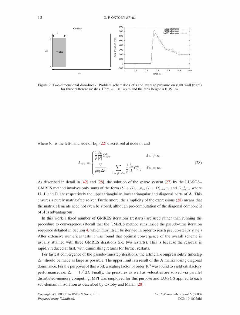
Figure 2. Two-dimensional dam-break: Problem schematic (left) and average pressure on right wall (right)for three different meshes. Here, a = 0.146 m and the tank height is 0.351 m.

where bm is the left-hand side of Eq. (22) discretised at node m and

Amn =

1

ρ

ℓk|ℓ|

Ckmn if n 6= m

V

ρc2τ∆τ−

∑

Υmq∩Vm

1

ρ

ℓk|ℓ|

Ckmq if n = m.

(28)

As described in detail in [42] and [28], the solution of the sparse system (27) by the LU-SGS–

GMRES method involves only sums of the form (U +D)mnvn, (L+D)mnvn and D−1mnvn where

U, L and D are respectively the upper trianglular, lower triangular and diagonal parts of A. This

ensures a purely matrix-free solver. Furthermore, the simplicity of the expressions (28) means that

the matrix elements need not even be stored, although pre-computation of the diagonal component

of A is advantageous.

In this work a fixed number of GMRES iterations (restarts) are used rather than running the

procedure to convergence. (Recall that the GMRES method runs inside the pseudo-time iteration

sequence detailed in Section 4, which must itself be iterated in order to reach pseudo-steady state.)

After extensive numerical tests it was found that optimal convergence of the overall scheme is

usually attained with three GMRES iterations (i.e. two restarts). This is because the residual is

rapidly reduced at first, with diminishing returns for further restarts.

For fastest convergence of the pseudo-timestep iterations, the artificial-compressibility timestep

∆τ should be made as large as possible. The upper limit is a result of the A matrix losing diagonal

dominance. For the purposes of this work a scaling factor of order 105 was found to yield satisfactory

performance, i.e. ∆τ = 105∆t. Finally, the pressures as well as velocities are solved via parallel

distributed-memory computing. MPI was employed for this purpose and LU-SGS applied to each

sub-domain in isolation as described by Oxtoby and Malan [28].




5. APPLICATION AND RESULTS

5.1. Mesh convergence: Two-dimensional dam-break

In this experiment, carried out by Martin and Moyce [43] an essentially 2D tank is divided in two,

with the left compartment containing water (as shown in the left panel of Fig. 2). Dynamics are

initiated by the sudden removal of the division, causing the water column to collapse. Viscous

(no-slip) boundaries were employed at all walls, with an outflow condition at the top of the tank

(fixed pressure and zero velocity gradient). The analyses were conducted on structured meshes,

the coarsest of which contains 42× 31 elements. The intermediate mesh has twice the number of

elements in both directions and for the fine mesh, the spacing is halved again. Simulations were

performed with Courant number Cf = 0.2.

Table I. Peak value of average pressure on right sidewall for two-dimensional dam-break problem on coarse,medium and fine grids.

Mesh density (elements) Peak pressure (Pa)

42× 31 727.784× 62 647.8

168× 124 623.4

In the right panel of Fig. 2 the spatially averaged pressure exerted on the right-hand wall is plotted

as a function of time (where atmospheric pressure at the top of the tank is set to zero). For the

purpose of assessing mesh convergence, the peak pressure is measured as shown in Table I for the

three meshes. The order of convergence is established from

p = ln

(

p2 − p1p3 − p2

)

/ ln(r),

where r = 2 in this case and p1, p2 and p3 are the peak pressure values for the coarse, intermediate

and fine meshes respectively [44]. This yields a convergence rate of p = 1.70, consistent with the

second-order spatial accuracy of the equations in the liquid and gas regions. Due to the fact that

the interface extends over more than one cell, the spatial accuracy in the region of the interface is

reduced, resulting in the overall convergence rate being less than 2.

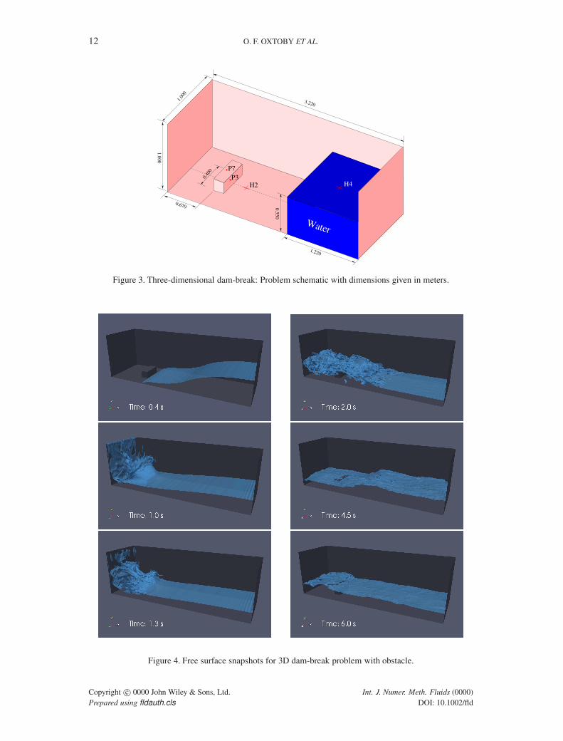
5.2. Validation: Three-dimensional dam-break

For the purposes of validation, we consider an experiment that was performed in a water-tank where

a released column of water strikes an obstacle affixed to the floor (representing a shipping container).

The experiment was reported by Kleefsman et al. [5, 45] along with numerical solutions. The

experiment has also been numerically modelled by Park et al. [17]. A schematic of the problem

with dimensions is shown in Fig. 3. The obstacle affixed to the floor has a square cross-section

of 0.16 m × 0.16 m. The water column is contained by a door which is suddenly removed. A

non-uniform structured mesh with 800 000 cells was employed, with viscous (no-slip) boundary

conditions applied at all walls, and with the open top being modelled by imposing a fixed (zero)

atmospheric pressure and zero gradient of velocity. Snapshots of the simulated free-surface are

shown in Fig. 4, showing the highly dynamic nature of the problem. For this reason a smaller

Courant number Cf = 0.1 was used for this problem, as numerical smearing of the interface was




0.670

1.00

0

1.220

1.0

00

0.5

50

3.220

H2P3

P7

0.40

0

H4

Water

Figure 3. Three-dimensional dam-break: Problem schematic with dimensions given in meters.

Figure 4. Free surface snapshots for 3D dam-break problem with obstacle.




-0.05

0

0.05

0.1

0.15

0.2

0.25

0.3

0.35

0.4

0.45

0 1 2 3 4 5 6

Hei

ght (

m)

Time (s)

ExperimentNumerical

0.1

0.15

0.2

0.25

0.3

0.35

0.4

0.45

0.5

0.55

0.6

0 1 2 3 4 5 6

Hei

ght (

m)

Time (s)

ExperimentNumerical

Figure 5. Three-dimensional dam-break problem: Comparison of experimental [5] and predicted evolutionof the water surface height above probe H2 (left pane) and H4 (right pane).

-1000

0

1000

2000

3000

4000

5000

6000

7000

0 1 2 3 4 5 6

Pre

ssur

e (P

a)

Time (s)

ExperimentNumerical

-1000

0

1000

2000

3000

4000

5000

6000

0 1 2 3 4 5 6

Pre

ssur

e (P

a)

Time (s)

ExperimentNumerical

Figure 6. Three-dimensional dam-break problem: Comparison of experimental [5] and predicted evolutionof pressure at probes P3 (left pane) and P7 (right pane).

observed for larger values. Note that no surface-tension or bubble-formation models are considered

in this paper.

For validation purposes, we compare the water heights measured above probes H2 and H4 (Fig.

3), with those predicted (see Fig. 5). The height probes are located at the centre of the box, with H2

being 1.000 m from the left sidewall and H4 being 0.560 m from the right sidewall. In addition to

the height measurements, there are pressure probes embedded in the obstacle. Probe P3 is located

on its front surface (facing the water column) at a height of 0.099 m from the bottom floor and offset

0.026 m left of centre if the obstacle is viewed from the front surface. Probe P7 is situated on the

top of the obstacle, 0.097 m behind the front surface and offset 0.026 m to the right of its centre.

Looking at the height measurements in Fig. 5, the results agree well with experiment except

for some noise in the H2 measurement between roughly 1 and 2.5 seconds. The rapid oscillation

in H2 occurs during a period of violent agitation as seen in Fig. 4, and it is not certain how the

experimentally determined water height was defined in this case. There is no discernable phase-

shift in the return wave which occurs at approximately 4.5 s in the plot of H2. As for the pressure

measurements in Fig. 6, note in particular the accurate prediction of peak pressure in the impact of

the initial wave with the front of the obstacle.




Linear speedupSpeedup per iterationNumber of iterations

Number of processors

Num

ber

of

iter

atio

ns

Spee

dup

20

15

10

5

0

140120100806040200

140

120

100

80

60

40

20

0

Figure 7. Parallelisation speed-up for the 3D dam-break problem considered in Section 5.2. The right-handaxis depicts the number of iterations required per time-step.

5.3. Parallel Performance

The parallel efficiency of the code was assessed by application to the 3D dam-break problem

described above. Execution time for the second timestep of the problem, of size ∆t = 0.005 s,

was compared. The time measurement was accomplished by timers embedded in the code and

included all computation of both the explicit momentum and interface tracking equations as well as

the implicitly solved pressure equation, but excluded any time taken to write output files. Results

presented are the average of five separate executions of the code. Calculations were performed

on a Sun Microsystems Constellation cluster with 8-core Intel Nehalem 2.9 GHz processors and

Infiniband interconnects at the Centre for High Performance Computing (CHPC), Cape Town.

The results of the study are depicted in Fig. 7, where the number of iterations achieved per

second has been divided by the value for a single processor to give the computational speedup

per iteration. As shown, super-linear speed-up is demonstrated, with very close to linear speed-up at

up to 120 cores. Note that, as a consequence of the preconditioning being done block-for-block on

each parallel subdomain, the number of iterations taken to converge the time-step is not constant,

and is also plotted in Fig. 7. As seen, this does not show a deteriorating trend as one might expect.

5.4. Application: Two-dimensional violent sloshing

The next test-case considered is a sloshing problem in two dimensions but featuring sustained

resonant excitation and, as a consequence, highly dynamic free-surface motion. The experimental

setup consists of a tank with a baffle in the middle, as detailed in Fig. 8, initially filled with water

to 25% of the tank height. The tank is subjected to the acceleration also plotted in Fig. 8, namely

a ramped sinusoid with a peak amplitude of 5.99 m s−2. The experimental results were generated

by the Bristol Earthquake and Engineering Laboratory Ltd at the Bristol Laboratories for Advanced

Dynamic Engineering (BLADE), University of Bristol.




-0.8

-0.6

-0.4

-0.2

0

0.2

0.4

0.6

0.8

0 2 4 6 8 10 12

Acc

eler

atio

n (g

)

Time (s)

Figure 8. Experimental configuration (top left) showing positions of pressure-probes, applied lateralacceleration (top right), and coarse hybrid-unstructured mesh (bottom) with 7 000 nodes.

The small gaps in the baffle and the violence of the sloshing make this a difficult problem

to resolve numerically. The numerical calculations were performed with a Courant number of

Cf = 0.05 in order to reduce numerical smearing of the interface under highly violent sloshing

conditions. Figure 8 shows the coarser of the two hybrid-unstructured meshes used, containing

7 000 cells. The finer mesh, containing 27 000 cells, is the same but with the mesh spacing halved

throughout.

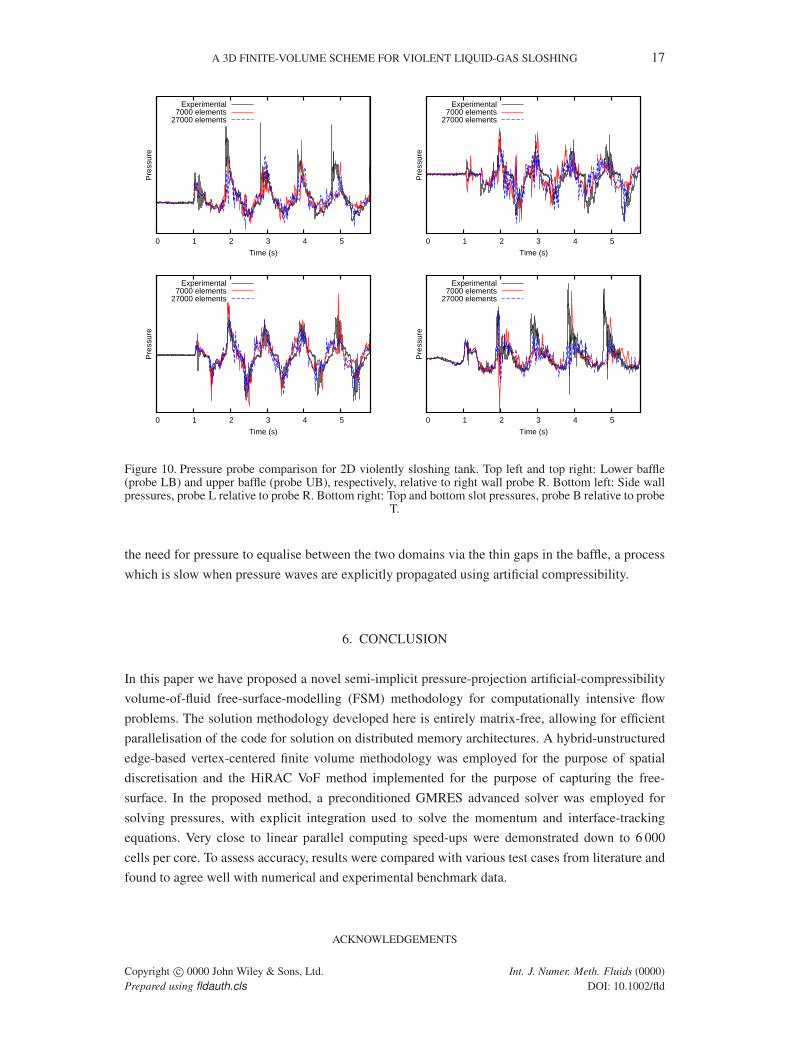
Figure 9 shows a comparison of snapshots of the free-surface interface in the experiment

and numerical simulation, showing a good correlation of large-scale structures. A comparison of

measured and predicted pressure values is additionally shown in Fig. 10. The locations of these

measurements are the probe locations depicted in Fig. 8. Note that all pressures shown are relative

pressures between two points in the tank, as incompressible solvers can only predict pressure

differences and not absolute pressures. The relative loading on the two sidewalls is shown, as

well as on each baffle element relative the right hand sidewall. Additionally the relative pressure

between the probes ‘B’ and ‘T’ located near the lowest and highest slots is plotted. For comparison,

results are presented for the 7 000 element hybrid-unstructured mesh as well as a fine 27 000 element

mesh. There is no clear increase in accuracy for the fine mesh, indicating that the inaccuracy in the

results does not stem primarily from inadequate mesh resolution. Moreover, a reasonable to good

correlation was achieved with experimental data for lower frequency high-amplitude pressures. This

is particularly the case for the lower-baffle and side-wall pressures.

To assess the effect of the LU-SGS-preconditioned GMRES advanced solver referred to

previously, the problem above was run until 1.0 s of simulation time on the 6 000 cell mesh to reach

a representative timestep, and the time taken to solve the subsequent timestep measured using the

advanced solver for the pressure equation compared to explicit Jacobi with artificial compressibility.

The former was 400 times faster, a particularly extreme speedup for this particular problem due to




Figure 9. Free-surface interface plots for 2D violently sloshing tank, showing numerical snapshots belowphotographs of the experiment.




0 1 2 3 4 5

Pre

ssur

e

Time (s)

Experimental7000 elements

27000 elements

0 1 2 3 4 5

Pre

ssur

e

Time (s)


27000 elements

0 1 2 3 4 5

Pre

ssur

e

Time (s)


27000 elements

0 1 2 3 4 5P

ress

ure

Time (s)


27000 elements

Figure 10. Pressure probe comparison for 2D violently sloshing tank. Top left and top right: Lower baffle(probe LB) and upper baffle (probe UB), respectively, relative to right wall probe R. Bottom left: Side wallpressures, probe L relative to probe R. Bottom right: Top and bottom slot pressures, probe B relative to probe

T.

the need for pressure to equalise between the two domains via the thin gaps in the baffle, a process

which is slow when pressure waves are explicitly propagated using artificial compressibility.

6. CONCLUSION

In this paper we have proposed a novel semi-implicit pressure-projection artificial-compressibility

volume-of-fluid free-surface-modelling (FSM) methodology for computationally intensive flow

problems. The solution methodology developed here is entirely matrix-free, allowing for efficient

parallelisation of the code for solution on distributed memory architectures. A hybrid-unstructured

edge-based vertex-centered finite volume methodology was employed for the purpose of spatial

discretisation and the HiRAC VoF method implemented for the purpose of capturing the free-

surface. In the proposed method, a preconditioned GMRES advanced solver was employed for

solving pressures, with explicit integration used to solve the momentum and interface-tracking

equations. Very close to linear parallel computing speed-ups were demonstrated down to 6 000

cells per core. To assess accuracy, results were compared with various test cases from literature and

found to agree well with numerical and experimental benchmark data.

ACKNOWLEDGEMENTS




We are grateful to Airbus UK Ltd, in particular Dale King and Francesco Gambioli, for supporting this

work as well as for valuable technical insight. We acknowledge the Bristol Laboratories for Advanced

Dynamic Engineering (BLADE) at the University of Bristol for experimental results, and thank Airbus UK

for permission to reproduce them. This work was also funded by the Council for Scientific and Industrial

Research (CSIR) on Thematic Type A Grant no. TA-2009-013. Finally, we would like to acknowledge the

Centre for High Performance Computing (CHPC) for access to computing hardware.

REFERENCES

1. Ibrahim RA. Liquid Sloshing Dynamics: Theory and Applications. Cambridge University Press: New York, 2005.

2. Lohner R, Yang C, Onate E. Simulation of flows with violent free surface motion and moving objects using

unstructured grids. International Journal For Numerical Methods In Fluids 2007; 53:1315–1338.

3. Gerrits J, Veldman AEP. Dynamics of liquid-filled spacecraft. Journal of Engineering Mathematics 2003; 45:21–38.

4. Andrillon Y, Alessandrini B. A 2D+T VOF fully coupled formulation for the calculation of breaking free-surface

flow. Journal of Marine Science and Technology 2004; 8:159–168, doi:10.1007/s00773-003-0167-1.

5. Kleefsman KMT, Fekken G, Veldman AEP, Iwanowski B, Buchner B. A volume-of-fluid simulation method for

wave impact problems. Journal of Computational Physics 2005; 206:363–393.

6. Brennan D. The numerical simulation of two-phase flows in settling tanks. PhD Thesis, Imperial College of Science,

Technology and Medicine, University of London 2001.

7. Mao ZS, Dukler AE. An experimental study of the collapse of gas–liquid slug flow. Experiments in Fluids 1989;

8:169–182.

8. Ozkan F, Worner M, Wenka A, Soyhan HS. Critical evaluation of CFD codes for interfacial simulation of bubble-

train flow in a narrow channel. International Journal For Numerical Methods In Fluids 2007; 55:537–564.

9. Harlow FH, Welch JE. Numerical calculation of time–dependent viscous incompressible flow of fluid with free

surface. The Physics of Fluids 1965; 8(12):2182–2189.

10. Ferziger JH, Peric M. Computational Methods for Fluid Dynamics. Springer-Verlag: New York, 1999.

11. Hirt CW, Nichols BD. Volume of fluid (VOF) method for the dynamics of free boundaries. Journal of

Computational Physics 1981; 39:201–225.

12. Ubbink O. Numerical prediction of two fluid systems with sharp interfaces. PhD Thesis, Imperial College of

Science, Engineering and Technology, University of London 1997.

13. Rider WJ, Kothe DB. Reconstructing volume tracking. Journal of Computational Physics 1998; 141:112–152.

14. Ubbink O, Issa RI. A method for capturing sharp fluid interfaces on arbitrary meshes. Journal of Computational

Physics 1999; 153:26–50.

15. Osher S, Sethian JA. Fronts propagating with curvature dependent speed: algorithms based on Hamilton–Jacobi

formulations. Journal of Computational Physics 1988; 79:12–49.

16. Wang Z, Yang J, Koo B, Stern F. A coupled level set and volume-of-fluid method for sharp interface simulation of

plunging breaking waves. International Journal of Multiphase Flow 2009; 35:227–246.

17. Park IR, Kim KS, Kim J, Van SH. A volume-of-fluid method for incompressible free surface flows. International

Journal for Numerical Methods in Fluids 2009; 61:1331–1362.

18. Heyns JA, Malan AG, Harms TM, Oxtoby OF. Development of a compressive surface capturing formulation for

modelling free-surface flow using the volume-of-fluid approach. International Journal for Numerical Methods in

Fluids 2013; 71:788–804, doi:10.1002/fld.3694.

19. Jasak H, Weller H. Interface tracking capabilities of the Inter–Gamma differencing scheme. Technical Report, CFD

research group, Imperial College, London 1995.

20. Malan AG, Lewis RW, Nithiarasu P. An improved unsteady, unstructured, artificial compressibility, finite volume

scheme for viscous incompressible flows: Part I. Theory and implementation. International Journal for Numerical

Methods in Engineering 2002; 54(5):695–714.

21. Malan AG, Lewis RW, Nithiarasu P. An improved unsteady, unstructured, artificial compressibility, finite volume

scheme for viscous incompressible flows: Part II. Application. International Journal for Numerical Methods in

Engineering 2002; 54(5):715–729.

22. Lewis RW, Malan AG. Continuum thermodynamic modeling of drying capillary particulate materials via an edge-

based algorithm. Computer Methods in Applied Mechanics and Engineering 2005; 194(18–20):2043–2057, doi:

10.1016/j.cma.2003.08.017.




23. Pattinson J, Malan AG, Meyer JP. A cut-cell non-conforming cartesian mesh method for compressible and

incompressible flow. International Journal for Numerical Methods in Engineering 2007; 72(11):1332–1354.

24. Malan AG, Meyer JP, Lewis RW. Modelling non-linear heat conduction via a fast matrix-free implicit unstructured-

hybrid algorithm. Computer Methods in Applied Mechanics and Engineering 2007; 196(45-48):4495–4504.

25. Malan AG, Lewis RW. An artificial compressibility CBS method for modelling heat transfer and fluid flow in

heterogeneous porous materials. International Journal for Numerical Methods in Engineering 2011; 87(1–5):412–

423, doi:10.1002/nme.3125.

26. Malan AG, Oxtoby OF. An accelerated, fully-coupled, parallel 3d hybrid finite-volume fluid-structure interaction

scheme. Computer Methods in Applied Mechanics and Engineering 2013; 253:426–438, doi:10.1016/j.cma.2012.

09.004.

27. Lohner R. Applied CFD Techniques. John-Wiley and Sons Ltd.: Chichester, 2001.

28. Oxtoby OF, Malan AG. A matrix-free, implicit, incompressible fractional-step algorithm for fluid–structure

interaction applications. Journal of Computational Physics 2012; 231:5389–5405, doi:http://dx.doi.org/10.1016/

j.jcp.2012.04.037.

29. Panahi R, Jahanbakhsh E, Seif MS. Development of a VoF-fractional step solver for floating body motion

simulation. Applied Ocean Research 2006; 28:171–181.

30. Lin LU, Yu-cheng LI, Bin T. Numerical simulation of turbulent free surface flow over obstruction. Journal of

Hydrodynamics 2008; 20(4):414–423.

31. Liu D, Lin P. Three-dimensional liquid sloshing in a tank with baffles. Ocean Engineering 2009; 36:202–212.

32. Liu J, Koshizuka S, Oka Y. A hybrid particle-mesh method for viscous, incompressible, multiphase flows. Journal

of Computational Physics 2005; 202:65–93.

33. Wacławczyk T, Koronowicz T. Modeling of the wave breaking with CICSAM and HRIC high-resolution schemes.

ECCOMAS CFD 2006: Proceedings of the European Conference on Computational Fluid Dynamics, Wesseling S,

Onate E, Periaux J (eds.), Delft University of Technology, 2006.

34. Zhao Y, Zhang B. A high-order characteristics upwind FV method for incompressible flow and heat transfer

simulation on unstructured grids. International Journal for Numerical Methods in Engineering 1994; 37:3323–

3341.

35. van Leer B. Towards the ultimate conservative difference scheme IV: A new approach to numerical convection.

Journal of Computational Physics 1977; 23:276–299.

36. Crumpton PI, Moinier P, Giles MB. An unstructured algorithm for high Reynolds number flows on highly stretched

meshes. Numerical Methods in Laminar and Turbulent Flow, Taylor C, Cross JT (eds.), Pineridge Press, 1997;

561–572.

37. Lohner R, Yang C, Cebral J, Camelli F, Soto O, Waltz J. Improving the speed and accuracy of projection-type

incompressible flow solvers. Computer Methods in Applied Mechanics and Engineering 2006; 195:3087–3109.

38. Nithiarasu P. An efficient artificial compressibility (AC) scheme based on the characteristic based split (CBS)

method for incompressible flow. International Journal for Numerical Methods in Engineering 2003; 56(13):1815–

1845.

39. Nithiarasu P. An arbitrary Lagrangian Eulerian (ALE) formulation for free surface flows using the characteristic-

based split (CBS) scheme. International Journal for Numerical Methods in Fluids 2005; 48:1415–1428.

40. Blazek J. Computational Fluid Dynamics: Principles and Applications. First edition. edn., Elsevier Science:

Oxford, 2001.

41. Saad Y, Schultz MH. GMRES: A generalized mimimal residual algorithm for solving nonsymmetric linear systems.

SIAM Journal on Scientific and Statistical Computing 1986; 7(3):856–869.

42. Luo H, Baum JD, Lohner R. A fast, matrix-free implicit method for compressible flows on unstructured grids.

Journal of Computational Physics 1998; 146:664–690.

43. Martin JC, Moyce WJ. An experimental study of the collapse of a liquid column on a rigid horizontal plane.

Philosophical Transactions of the Royal Society of London, Series A 1952; 244:312–324.

44. Roache P. Verification of codes and calculations. AIAA Journal 1998; 36:696–702.

45. Kleefsman KMT. Water impact loading on offshore structures. a numerical study. PhD Thesis, Rijksuniversiteit

Groningen 2005.



Documents

A computationally efﬁcient 3D ﬁnite-volume scheme for