A Computational Model of Logical Metonymy - cl.cam.ac.ukes407/papers/TSLP-LogMet.pdf · A Computational Model of Logical Metonymy 11:3 2. THEORETICAL BACKGROUND Regular polysemy in

11

A Computational Model of Logical Metonymy

EKATERINA SHUTOVA, JAKUB KAPLAN, SIMONE TEUFEL, and ANNA KORHONEN,University of Cambridge

The use of figurative language is ubiquitous in natural language texts and it is a serious bottleneck in au-tomatic text understanding. A system capable of interpreting figurative expressions would be an invaluableaddition to the real-world natural language processing (NLP) applications that need to access semantics,such as machine translation, opinion mining, question answering and many others. In this article we focuson one type of figurative language, logical metonymy, and present a computational model of its interpreta-tion bringing together statistical techniques and the insights from linguistic theory. Compared to previousapproaches this model is both more informative and more accurate. The system produces sense-level inter-pretations of metonymic phrases and then automatically organizes them into conceptual classes, or roles,discussed in the majority of linguistic literature on the phenomenon.

Categories and Subject Descriptors: H.3.1 [Information Storage and Retrieval]: Content Analysis andIndexing

General Terms: Algorithms, Experimentaion, Languages

Additional Key Words and Phrases: Logical metonymy, semantic interpretation, word sense disambiguation

ACM Reference Format:Shutova, E., Kaplan, J., Teufel, S., and Korhonen, A. 2013. A computational model of logical metonymy. ACMTrans. Speech Lang. Process. 10, 3, Article 11 (July 2013), 28 pages.DOI: http://dx.doi.org/10.1145/2483969.2483973

1. INTRODUCTION

Metonymy is defined as the use of a word or a phrase to stand for a related concept,that is not explicitly mentioned. It is based on contiguity between the concepts andimplies a contact or a rather physical connection between the entities. The followingare some examples of metonymic phrases.

(1) The pen is mightier than the sword. [Bulwer-Lytton 1839](2) He played Bach.(3) He drank his glass. [Fass 1991](4) Thank you for the present! I really enjoyed your book.(5) John is enjoying his cigarette outside.(6) After three martinis John was feeling well. [Godard and Jayez 1993]

The metonymic adage in (1) is a classical example. Here the pen stands for the pressand the sword for military power. In (2) Bach is used to refer to the composer’s musicand in (3) the glass stands for its content, that is the actual drink (beverage). These

Authors’ address: Computer Laboratory, William Gates Building, 15 JJ Thomson Avenue, Cambridge CB30FD, UK; email: {Ekaterina.Shutova, Simone.Teufel, Anna.Korhonen}@cl.cam.ac.uk, [email protected] to make digital or hard copies of part or all of this work for personal or classroom use is grantedwithout fee provided that copies are not made or distributed for profit or commercial advantage and thatcopies show this notice on the first page or initial screen of a display along with the full citation. Copyrights forcomponents of this work owned by others than ACM must be honored. Abstracting with credit is permitted.To copy otherwise, to republish, to post on servers, to redistribute to lists, or to use any component of thiswork in other works requires prior specific permission and/or a fee. Permissions may be requested fromPublications Dept., ACM, Inc., 2 Penn Plaza, Suite 701, New York, NY 10121-0701 USA, fax +1 (212)869-0481, or [email protected]© 2013 ACM 1550-4875/2013/07-ART11 $15.00

DOI: http://dx.doi.org/10.1145/2483969.2483973

ACM Transactions on Speech and Language Processing, Vol. 10, No. 3, Article 11, Publication date: July 2013.

11:2 E. Shutova et al.

are examples of general metonymy. The sentences (4–6) represent a variation of thisphenomenon called logical metonymy. Here both your book, his cigarette and threemartinis have eventive interpretations, that is the noun phrases stand for the eventsof reading the book, smoking the cigarette and drinking three martinis respectively.

General metonymy is traditionally explained via conventionalized metonymic pat-terns that operate over semantic classes [Stern 1931; Lakoff and Johnson 1980; Fass1997]. The following are some examples of common metonymic patterns.

—PART-FOR-WHOLE (also known as synechdoche), for example, “I could do with anextra pair of hands” (referring to a helper or a worker).

—CONTAINER-FOR-CONTENTS, for example, “He drank his glass.”—PRODUCER-FOR-PRODUCT, for example, “I bought a Picasso.”—PLACE-FOR-EVENT, for example, “at the time of Vietnam, increased spending led

to inflation and trade deficit” [Markert and Nissim 2006].—PLACE-FOR-PRODUCT, for example, “He drinks Bordeaux with his dinner.”—PLACE-FOR-INHABITANTS, for example, “France is on strike again.”—ORGANIZATION-FOR-MEMBERS, for example, “Last February NASA announced

[. . . ]” [Markert and Nissim 2006].—OBJECT USED-FOR-USER, for example, “The sax has a flu today.”

Such pattern-based shifts in meaning happen systematically and are known as reg-ular polysemy [Apresjan 1973], or sense extension [Copestake and Briscoe 1995]. How-ever, some metonymic examples emerge only in specific contexts and are less conven-tionalized than others. Markert and Nissim [2006] call metonymies such as those in(7) and (8) unconventional.

(7) The ham sandwich is waiting for his check. [Nunberg 1978](8) Ask seat 19 whether he wants to swap. [Markert and Nissim 2006]

These examples illustrate that metonymy is both regular and productive.As well as general metonymy, logical metonymy is an elliptical construction, that is it

lacks an element that is recoverable or inferable from the context. However, if generalmetonymies usually follow a certain conceptual pattern (such as one of the preceding),logical metonymy arises due to a predicate taking syntactic and semantic argumentsof different types. For example, the verb enjoy in (4) requires an event as its semanticargument (it is a process that one enjoys), but also allows for an object expressed bya noun phrase syntactically. Thus the noun phrase your book in (4) is interpreted as“reading your book.” But how would one know that enjoy a book means enjoy reading abook and enjoy a cigarette means enjoy smoking a cigarette, and not for example, enjoybuying a book, or enjoy smoking a book, or enjoy eating a cigarette? Humans are capableof interpreting these phrases using their world knowledge and contextual information.Modelling this process is the focus of our experiments.

The fact that logical metonymy is both highly frequent and productive makes its com-putational processing an important problem within NLP. In this article, we focus on theproblem of interpretation of logical metonymy and adopt a statistical data-driven ap-proach to it. Our system first derives a set of possible metonymic interpretations froma large corpus. It then disambiguates them with respect to their word sense, using anexisting sense inventory, and automatically organizes them into a new class-based con-ceptual model of logical metonymy that is inspired by linguistic theory [Vendler 1968;Pustejovsky 1991; Godard and Jayez 1993]. We then experimentally verify whether thisrepresentation is intuitive to humans, by asking human subjects to classify metonymicinterpretations into groups of similar concepts.


A Computational Model of Logical Metonymy 11:3

2. THEORETICAL BACKGROUND

Regular polysemy in general and logical metonymy in particular have long been ofconsiderable interest for lexical semantics. The term logical metonymy captures arange of phenomena where a noun phrase is used to stand for an event associatedwith this noun phrase. The following are a few examples of logical metonymic phrases(under (a)) and their usual interpretations (under (b)).

(9) a. Mark enjoyed this book.b. Mark enjoyed reading this book.

(10) a. Mark always enjoys his beer.b. Mark always enjoys drinking his beer.

(11) a. Mark enjoyed his cigarette.b. Mark enjoyed smoking his cigarate

(12) a. Mark enjoyed the cake.b. Mark enjoyed eating the cake.

(13) a. Mark enjoyed the concert.b. Mark enjoyed listening to the concert.

(14) a. a good mealb. a meal that tastes good

(15) a. a good cookb. a cook that cooks well

(16) a. After the movie Mark went straight to bed.b. After watching the movie Mark went straight to bed.

(17) a. After three martinis Mark was feeling well.b. After drinking three martinis Mark was feeling well.

(18) a. After the lecture Mark looked tired.b. After listening to the lecture Mark looked tired.

In all of these phrases a shift of meaning happens in a systematic way. The metonymicverb or preposition semantically selects for an argument of type event, but however,is combined with a noun phrase syntactically. This is metonymy in the sense thatone phrase is used to stand for another related one, and it is, logical because it istriggered by semantic type constraints that the verb, adjective, or preposition placesonto its arguments. This is known in linguistics as a phenomenon of type coercion.Many existing approaches to logical metonymy explain systematic syntactic ambiguityof metonymic verbs (such as enjoy) or prepositions (such as after) by means of typecoercion [Pustejovsky 1991; 1995; Briscoe et al. 1990; Verspoor 1997; Godard and Jayez1993]. The actual interpretations (events), according to these approaches, are suggestedby lexical defaults associated with the noun in the complement. Within his GenerativeLexicon theory, Pustejovsky [1991] models these lexical defaults in the form of thequalia structure of the noun. As set out by Pustejovsky the qualia structure of a nounspecifies the following aspects of its meaning.

—CONSTITUTIVE Role (the relation between an object and its constituents, e.g. pages,cover for book);

—FORMAL Role (that which distinguishes the object within a larger domain, e.g.physical object for book);

—TELIC Role (purpose and function of the object, e.g. read for book);—AGENTIVE Role (how the object came into being, e.g. write for book).

Qualia structure plays an important role in the interpretation of different kinds ofmultiword expressions, most prominent of them being compound nouns (e.g. cheeseknife is a knife for cutting cheese) and logical metonymy. For the problem of logical



metonymy telic and agentive roles are of particular interest. For example, the nounbook would have read specified as its telic role and write as its agentive role in itsqualia structure. Lexical defaults are inherited within the semantic class hierarchyand are activated in the absence of contradictory pragmatic information [Briscoe et al.1990]. For example, all the nouns belonging to the class LITERATURE (e.g. book, story,novel, etc.) will have read specified as their telic role. In some cases lexical defaultscan, however, be overridden by context. Consider the following example taken fromLascarides and Copestake [1995].

(19) My goat eats anything. He really enjoyed your book.

Here it is clear that “the goat enjoyed eating the book” and not “reading the book”,which is enforced by the context. Such cases, however, are rare.

This shows that logical metonymy is both conventionalized (e.g. conventional telicinterpretations such as “enjoy reading the book”), as well as productive, that is newmetonymic interpretations emerge outside of ordinary context, as in (19). A number ofapproaches discuss semiproductivity of the phenomenon [Copestake and Briscoe 1995;Copestake 2001]. Not all nouns that have evident telic and agentive roles can be equallycombined with aspectual verbs. Consider the following examples.

(20) *John enjoyed the dictionary.(21) *John enjoyed the door.(22) *John began the tree.

These examples suggest that there are certain conventional constraints on re-alisation and interpretation of logical metonymy. Such constraints were discussedin a number of studies [Pustejovsky 1991; Godard and Jayez 1993; Pustejovskyand Bouillon 1995; Copestake and Briscoe 1995; Verspoor 1997; Copestake 2001].However, in reality the interpretation of logical metonymy (like any other linguisticphenomenon) is also a matter of pragmatics, that is one can often imagine a possiblesituation in which a particular phrase can be interpreted (e.g. an artist (John) begandrawing a tree interpretation of (22) and therefore, the validity of such examples isnever clear-cut. However, the goal of this article is to propose a computational methodcapable of interpreting more common logical metonymies, whose possible meaningscan be derived even in isolation from wider context and pragmatics.

While Pustejovsky’s treatment of logical metonymy within the Generative Lexicontheory evolves around the rich semantics of the head noun in the metonymic phrase,other approaches perceive linguistic constraints on interpretations as inherent to thesemantics of metonymic verbs [Copestake and Briscoe 1995; Pustejovsky and Bouillon1995]. Godard and Jayez [1993] claim that possible interpretations represent a kindof a modification to the object referred to by the noun phrase (NP), more specifically,that the object usually “comes into being”, “is consumed”, or “undergoes a change ofstate”. All of these approaches view metonymic interpretation at the level of individualwords, as opposed to Vendler [1968], who points out that in some cases a group of verbsis needed to fully interpret metonymic phrases. He gives examples of adjective-nounmetonymic constructions, for example, “fast scientist” can be interpreted as both “ascientist who does experiments quickly” and “publishes fast (and a lot)” at the sametime.

Verspoor [1997] conducted an empirical study of logical metonymy in real-world text.She explored the data regarding logical metonymy from the Lancaster Oslo/Bergen(LOB) Corpus1 and the British National Corpus for aspectual verbs begin and finish.

1http://khnt.hit.uib.no/icame/manuals/lob/INDEX.HTM.



She investigated how frequent the use of logical metonymy is for these verbs, as wellas how often the resulting constructions can be interpreted based on the head noun’squalia structure. Verspoor came to the conclusion that for these two aspectual verbsthe interpretation of logical metonymy is indeed restricted to either agentive events orconventionalized telic events associated with the noun complement and that the vastmajority of uses are conventional.

3. PREVIOUS COMPUTATIONAL APPROACHES

Along with theoretical work, there have been a number of computational accounts ofgeneral [Utiyama et al. 2000; Markert and Nissim 2002; Nissim and Markert 2003;Peirsman 2006; Agirre et al. 2007] and logical [Lapata and Lascarides 2003] metonymy.All of these approaches are data-driven. The majority of the approaches to general meto-nymy (with the exception of Utiyama et al. [2000]) deal only with metonymic propernames, use machine learning and treat metonymy resolution as classification accord-ing to common metonymic patterns. In contrast, Utiyama et al. [2000], followed byLapata and Lascarides [2003], used text corpora to automatically derive paraphrasesfor metonymic expressions. Utiyama et al. [2000] used a statistical model for the inter-pretation of general metonymies for Japanese. Given a verb-object metonymic phrase,such as read Shakespeare, they searched for entities the object could stand for, such asplays of Shakespeare. They considered all the nouns cooccuring with the object nounand the Japanese equivalent of the preposition of. Utiyama and his colleagues testedtheir approach on 75 metonymic phrases taken from the literature and report the re-sulting precision of 70.6%, whereby an interpretation was considered correct if it madesense in some imaginary context.

Lapata and Lascarides [2003] extend this approach to the interpretation of logicalmetonymies containing aspectual verbs (e.g. “begin the book”) and polysemous adjec-tives (e.g. “good meal” vs. “good cook”). The intuition behind their approach is similarto that of Pustejovsky [1991, 1995], namely that there is an event not explicitly men-tioned, but implied by the metonymic phrase (“begin to read the book”, or “the mealthat tastes good” vs. “the cook that cooks well”). They used the BNC parsed by the Cassparser [Abney 1996] to extract events (verbs) cooccuring with both the metonymic verbor adjective and the noun independently, and ranked them in terms of their likelihoodaccording to the data. The likelihood of a particular interpretation was calculated asfollows:

P(e, v, o) = f (v, e) · f (o, e)N · f (e)

, (1)

where e stands for the eventive interpretation of the metonymic phrase, v for themetonymic verb and o for its noun complement. f (e), f (v, e), and f (o, e) are the respec-tive corpus frequencies. N = ∑

i f (ei) is the total number of verbs in the corpus. Thelist of interpretations Lapata and Lascarides [2003] report for the phrase “finish video”is shown in Table I.

Lapata and Lascarides produced ranked lists of interpretations for 58 metonymicphrases. This dataset was compiled by selecting 12 verbs that allow logical metonymy2

from the lexical semantics literature and combining each of them with 5 nouns.This yields 60 phrases, which were then manually filtered, excluding 2 phrases asnonmetonymic.

They compared their results to paraphrase judgements elicited from humans. Thesubjects were presented with three interpretations for each metonymic phrase (fromhigh, medium, and low probability ranges) and were asked to associate a number with

2Attempt, begin, enjoy, finish, expect, postpone, prefer, resist, start, survive, try, want.



Table I. Interpretations of Lapata and Lascarides for “Finish Video”

Metonymic Phrase Interpretations Log-probabilityfinish video film −19.65

edit −20.37shoot −20.40view −21.19play −21.29stack −21.75make −21.95

programme −22.08pack −22.12use −22.23

watch −22.36produce −22.37

each of them reflecting how good they found the interpretation. They reported a correla-tion of 0.64, whereby the intersubject agreement was 0.74. It should be noted, however,that such an evaluation scheme is not very informative as Lapata and Lascarides cal-culate correlation only on 3 data points for each phrase out of many more yielded by themodel. It fails to take into account the quality of the list of top-ranked interpretations,although the latter is deemed to provide the right answer. In comparison, the fact thatLapata and Lascarides initially selected the interpretations from high, medium or lowprobability ranges makes achieving a high correlation between the model rankings andhuman judgements significantly easier.

4. ALTERNATIVE INTERPRETATION OF LOGICAL METONYMY

The approach of Lapata and Lascarides [2003] produces a list of nondisambiguatedverbs representing possible interpretations of a metonymic phrase. Some of them in-deed correspond to paraphrases that a human would give for the metonymic phrase(e.g. read for enjoy a book). However, to provide useful information to NLP applicationsdealing with semantics, this work can be improved on in two main ways.

—First, the lists of possible interpretations produced by the system of Lapata andLascarides need to be filtered. They contain a certain proportion of incorrect inter-pretations (e.g. build for enjoy book), as well as synonymous ones.

—Second, in order to obtain the actual meaning of the metonymic phrase, the interpre-tations need to be disambiguated with respect to their word sense. Using sense-basedinterpretations of logical metonymy as opposed to ambiguous verbs could benefitother NLP applications that rely on disambiguated text (e.g. for the tasks of in-formation retrieval [Voorhees 1998; Schutze and Pedersen 1995; Stokoe et al. 2003],question answering [Pasca and Harabagiu 2001], or machine translation [Chan et al.2007; Carpuat and Wu 2007]).

Thus we propose an alternative representation of interpretation of logical metonymyconsisting of a list of verb senses that map to WordNet synsets and develop a word sensedisambiguation method for this task. Besides performing word sense disambiguation(WSD), this method also allows us to filter out irrelevant interpretations yielded by themodel of Lapata and Lascarides. However, the list of nondisambiguated interpretationssimilar to the one Lapata and Lascarides produce is a necessary starting point inbuilding the sense-based representation. Discovering metonymic interpretations anddisambiguating them with respect to word sense is the focus of our first experiment.



The second issue we address in this article is the design of a class-based modelof logical metonymy and its verification against human judgements. The class-basedmodel of logical metonymy is both application-driven and theoretically grounded. NLPapplications would benefit from the class-based representation since it provides moreaccurate and generalized information about possible interpretations of metonymicphrases that can be adapted to particular contexts the phrases appear in. Class-basedmodels of semantics are frequently created and used in NLP [Clark and Weir 2002;Korhonen et al. 2003; Lapata and Brew 2004; Schulte im Walde 2006; O Seaghdha2010]. Verb classifications specifically have been used to support a number of NLPtasks, for example, machine translation [Dorr 1998], document classification [Klavansand Kan 1998], and subcategorization acquisition [Korhonen 2002]. Besides providingmeaningful generalizations over concepts, class-based models also improve the accu-racy of statistical generalizations over corpus data [Brown et al. 1992]. They addressthe issue of data sparseness, which is a bottleneck for statistical learning from limitedamounts of data.

The class-based model also takes into account the constraints on logical metonymypointed out in linguistics literature [Vendler 1968; Pustejovsky 1991, 1995; Godardand Jayez 1993; Verspoor 1997]. As a reminder, Pustejovsky [1991] explains the inter-pretation of logical metonymy by means of lexical defaults associated with the nouncomplement in the metonymic phrase. He models these lexical defaults in the form ofthe qualia structure of the noun, whereby telic and agentive roles are of particular rel-evance for logical metonymy. For example, the noun book would have read specified asits telic role and write as its agentive role in its qualia structure. Nevertheless, multipletelic and agentive roles can exist and be valid interpretations, as suggested by Verspoor[1997] and confirmed by the data of Lapata and Lascarides (see Table I). Therefore,we propose that these lexical defaults should be represented in the form of classes ofinterpretations (e.g. {read, browse, look through} vs. {write, compose, pen}) rather thansingle word interpretations (e.g. read and write) as suggested by Pustejovsky [1991].

Godard and Jayez [1993] view a metonymic interpretation as a modification to theobject referred to by the NP, that is the object “comes into being,” “is consumed,” or“undergoes a change of state.” This conveys an intuition that a sensible metonymicinterpretation should fall under one of those three classes. Comparing the interpreta-tions Lapata and Lascarides obtained for the phrase “finish video” (Table I), one canclearly distinguish between the meanings pertaining to the creation of the video, forexample, film, shoot, take, and those denoting using the video, for example, watch, view,see. However, the classes based on Pustejovsky’s telic and agentive roles do not explainthe interpretation of logical metonymy for all cases. Neither does the class divisionproposed by Godard and Jayez [1993]. For example, the most intuitive interpretationfor the metonymic phrase “he attempted the peak” is reach, which does not fall underany of these classes. It is hard to exhaustively characterize all possible classes of inter-pretations. Therefore, we treat this as an unsupervised clustering problem rather thana classification task and choose a theory-neutral data-driven approach to it. The objec-tive of our second experiment is to model the class division structure of metonymicinterpretations and experimentally verify whether the obtained data conformsto it.

In order to discover such classes, the interpretations are automatically clustered toidentify groups of related meanings. The automatic class discovery is carried out usingdisambiguated interpretations produced in the previous step. This is motivated by thefact that it is verb senses that form classes rather than polysemous verbs themselves.It is possible to model verb senses starting from nondisambiguated verbs using softclustering, that is a clustering algorithm that allows for one object to be part of different



clusters, as opposed to hard clustering, whereby each object can belong to one clusteronly. However, previous approaches to soft clustering of verbs have proved that this isa challenging task [Schulte im Walde 2000], whereas much success has ben achieved inhard clustering [Korhonen et al. 2003; Schulte im Walde 2006; Joanis et al. 2008; Sunand Korhonen 2009]. Thus in our experiments, we create verb clusters by performinghard clustering of verb senses instead of soft clustering of ambiguous verbs, and expectthis method to yield a better model of verb meaning. Clustering is performed using theinformation about lexico-syntactic environments, in which metonymic interpretationsappear, as features.

We start by reimplementing the method of Lapata and Lascarides [2003], and thenextend it by disambiguating the interpretations with respect to WordNet synsets forverb-object metonymic phrases. For this purpose, we develop a ranking scheme forthe synsets using a nondisambiguated corpus, address the issue of sense frequencydistribution and utilize information from WordNet glosses to refine the ranking. Inthe second experiment, the produced sense-based interpretations are automaticallyclustered based on their semantic similarity.

Both the disambiguation method and the class-based model are evaluated individu-ally against human judgements. Humans are presented with a set of verb senses thesystem produces as metonymic interpretations and asked to (1) remove the irrelevantinterpretations and (2) cluster the remaining ones. Their annotations are then usedfor the creation of a gold standard for the task. The performance of the system issubsequently evaluated against this gold standard.

5. EXTRACTING AMBIGUOUS INTERPRETATIONS

The method of Lapata and Lascarides [2003] is reimplemented to obtain a set of can-didate interpretations (ambiguous verbs) from a nonannotated corpus. However, ourreimplementation of the method differs from the system of Lapata and Lascarides inthat we use a more robust parser (RASP [Briscoe et al. 2006]), process a wider range ofsyntactic structures (coordination, passive), and extract our data from a later versionof the BNC. As a result, we expect our system to extract the data more accurately.

5.1. Parameter Estimation

The model of Lapata and Lascarides [2003] presented in Section 3 is used to create andrank the initial list of ambiguous interpretations. The parameters of the model wereestimated from the RASP-parsed BNC, using the grammatical relations (GR) outputof RASP for BNC created by Andersen et al. 2008. In particular, we extracted all directand indirect object relations for the nouns from the metonymic phrases, that is allthe verbs that take the head noun in the complement as an object (direct or indirect),in order to obtain the counts for f (o, e) from Lapata and Lascarides’ model. Relationsexpressed in the passive voice and with the use of coordination were also extracted. Theverb-object pairs attested in the corpus only once were discarded, as well as the verb be,since it does not add any semantic information to the metonymic interpretation. In thecase of indirect object relations, the verb was considered to constitute an interpretationtogether with the preposition, e.g. for the metonymic phrase “enjoy the city” the correctinterpretation is live in as opposed to live.

As the next step, the system identified all possible verb phrase (VP) complementsof the metonymic verb (both progressive and infinitive) that represent f (v, e). Thiswas done by searching for xcomp relations in the GRs output of RASP, in which themetonymic verb participates in any of its inflected forms. Infinitival and progressivecomplement counts were summed up to obtain the final frequency f (v, e).

After the frequencies f (v, e) and f (o, e) were obtained, possible interpretations wereranked according to the model of Lapata and Lascarides [2003]. The top interpretations



Table II. Possible Interpretations of Metonymies Ranked by Our System

finish video enjoy bookInterpretations Log-prob Interpretations Log-probview −19.68 read −15.68watch −19.84 write −17.47shoot −20.58 work on −18.58edit −20.60 look at −19.09film on −20.69 read in −19.10film −20.87 write in −19.73view on −20.93 browse −19.74make −21.26 get −19.90edit of −21.29 re-read −19.97play −21.31 talk about −20.02direct −21.72 see −20.03sort −21.73 publish −20.06look at −22.23 read through −20.10record on −22.38 recount in −20.13

for the metonymic phrases “enjoy book” and “finish video” together with their log-probabilities are shown in Table II.

5.2. Comparison with the Results of Lapata and Lascarides

We compared the output of our reimplementation of the model on Lapata and Las-carides’ dataset with their own results obtained from the authors. The major differencebetween the two systems is that we extracted the data from the BNC parsed by RASP,as opposed to the Cass chunk parser [Abney 1996] utilized by Lapata and Lascarides.Our system finds approximately twice as many interpretations as theirs and covers80% of their lists (the system fails to find only some of the low-probability range verbsof Lapata and Lascarides). We then compared the rankings of the two implementationsusing the Pearson correlation coefficient and obtained an average correlation of 0.83(over all metonymic phrases from the dataset of Lapata and Lascarides).

We evaluated the performance of the system against the judgements elicited from hu-mans in the framework of the experiment of Lapata and Lascarides [2003].3 The Pear-son correlation coefficient between the ranking of our system and the human rankingequals 0.62 (the intersubject agreement on this task is 0.74). This is slightly lower thanthe number achieved by Lapata and Lascarides (0.64). Such a difference is likely to becaused by the fact that our system does not find some of the low-probability range verbsthat Lapata and Lascarides included in their test set, and thus those interpretationsget assigned a probability of 0. In addition, we conducted a one-tailed t-test to deter-mine if the ranking scores obtained were significantly different from those of Lapataand Lascarides. The difference is statistically insignificant (t = 3.6; df = 180; p < .0005),and the output of the system is deemed acceptable to be used for further experiments.

5.3. Data Analysis

There has been a debate in linguistics literature as to whether it is the noun orthe verb in the metonymic phrase that determines the interpretation [Pustejovsky1991; Copestake and Briscoe 1995]. Pustejovsky’s theory of noun qualia explains thecontribution of the noun to the semantics of the whole phrase. However, it has alsobeen pointed out that different metonymic verbs also place their own requirementson the interpretation of logical metonymy [Godard and Jayez 1993; Pustejovsky and

3For a detailed description of the human evaluation setup see Lapata and Lascarides [2003], pp. 12–18.



Bouillon 1995; Copestake and Briscoe 1995]. We analyzed the sets of interpretationsfor metonymic phrases extracted from the corpus using the method of Lapata andLascarides [2003] with respect to such requirements. Our data suggests the followingclassification criteria for metonymic verbs.

—Control vs. raising. Consider the phrase “require poetry.” Require is a typical objectraising verb, and therefore the most obvious interpretation of this phrase wouldbe “require someone to learn/recite poetry,” rather than “require to hear poetry”or “require to learn poetry,” as suggested by the model of Lapata and Lascarides.Their model does not take into account raising syntactic frames and as such itsinterpretation of raising metonymic phrases will be based on the wrong kind ofcorpus evidence and lead to ungrammaticality. Our expectation, however, is thatcontrol verbs tend to form logical metonymies more frequently. By analyzing thelists of control and raising verbs compiled by Boguraev and Briscoe [1987] we foundevidence supporting this claim. According to our own judgements, only 20% of raisingverbs can form metonymic constructions (e.g. expect, allow, request, requires, etc.),while others cannot (e.g. appear, seem, consider, etc.) This finding complies with theview previously articulated by Pustejovsky and Bouillon [1995]. Due to both thisfinding and the fact that our experiments build on the approach of Lapata andLascarides [2003], we gave preference to control verbs when compiling a dataset todevelop and test the system.

—Activity vs. result. Some metonymic verbs require the reconstructed event to bean activity (e.g. begin writing the book), while others require a result (e.g. attempt toreach the peak). This distinction would potentially allow us to rule out some incorrectinterpretations, e.g. a resultative find for enjoy book, as enjoy requires an event ofthe type activity. Although we are not testing this hypothesis in the current work,automating this would be an interesting route for extension of our experiments inthe future.

—Telic vs. agentive vs. other events. Another interesting observation captures the con-straints that the metonymic verb imposes on the reconstructed event in terms of itsfunction. While some metonymic verbs require telic events (e.g., enjoy, want, try),others have strong preference for agentive (e.g. start). However, for some categoriesof verbs it is hard to define a particular type of the event they require (e.g. attemptthe peak should be interpreted as attempt to reach the peak, which is neither telicnor agentive).

6. DISAMBIGUATION EXPERIMENTS

The reimplementation of the method of Lapata and Lascarides produces interpreta-tions in the form of ambiguous strings representing collectively all senses of the verb.The aim is, however, to construct the list of verb senses that are correct interpretationsfor the metonymic phrase. We assume the WordNet synset representation of a senseand map the ambiguous interpretations to WordNet synsets. This is done by searchingthe obtained lists for verbs whose senses are in hyponymy and synonymy relationswith each other according to WordNet and recording the respective senses.

After word sense disambiguation of the interpretations is completed, one needs toderive a new likelihood ranking for the resulting senses. Since there is no word sensedisambiguated corpus available that would be large enough to reliably extract statisticsfor metonymic interpretations, the new ranking scheme is needed to estimate thelikelihood of a WordNet synset as a unit from a nondisambiguated corpus. We proposeto calculate synset likelihoods based on the initial likelihood of the ambiguous verbs,relying on the hypothesis of Zipfian sense frequency distribution and information fromWordNet glosses.



6.1. Generation of Candidate Senses

It has been recognized [Pustejovsky 1991; 1995; Godard and Jayez 1993] that correctinterpretations tend to form semantic classes, and therefore, they should be relatedto each other by semantic relations, such as synonymy or hyponymy. The right sensesof the verbs in the context of the metonymic phrase were obtained by searching theWordNet database for the senses of the verbs in the list that are in synonymy, hyper-nymy, and hyponymy relations and storing the corresponding synsets in a new list ofinterpretations. If one synset was a hypernym (or hyponym) of the other, then bothsynsets were stored.

For example, for the metonymic phrase “finish video,” the interpretations watch, view,and see are synonymous, therefore the synset containing (watch(3) view(3) see(7))was stored. This means that sense 3 of watch, sense 3 of view and sense 7 of see wouldbe correct interpretations of the metonymic expression.

The obtained number of synsets ranges from 14 (“try shampoo”) to 1216 (“wantmoney”) for the whole dataset of Lapata and Lascarides [2003].

6.2. Ranking the Senses

A problem arises with the obtained lists of synsets in that they contain different sensesof the same verb. However, few verbs have such a range of meanings that their twodifferent senses could represent two distinct metonymic interpretations (e.g., in caseof take interpretation of “finish video”, shoot sense and look at, consider sense are bothacceptable interpretations, the second obviously being dispreferred). In the majorityof cases the occurrence of the same verb in different synsets means that the list stillneeds filtering.

In order to do this, we rank the synsets according to their likelihood of being ametonymic interpretation. The sense ranking is based on the probabilities of the verbstrings derived by the model of Lapata and Lascarides [2003].

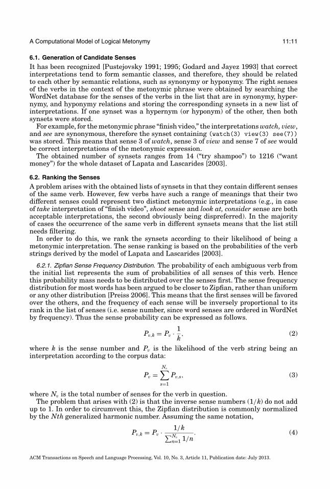
6.2.1. Zipfian Sense Frequency Distribution. The probability of each ambiguous verb fromthe initial list represents the sum of probabilities of all senses of this verb. Hencethis probability mass needs to be distributed over the senses first. The sense frequencydistribution for most words has been argued to be closer to Zipfian, rather than uniformor any other distribution [Preiss 2006]. This means that the first senses will be favoredover the others, and the frequency of each sense will be inversely proportional to itsrank in the list of senses (i.e. sense number, since word senses are ordered in WordNetby frequency). Thus the sense probability can be expressed as follows.

Pv,k = Pv · 1k, (2)

where k is the sense number and Pv is the likelihood of the verb string being aninterpretation according to the corpus data:

Pv =Nv∑

s=1

Pv,s, (3)

where Nv is the total number of senses for the verb in question.The problem that arises with (2) is that the inverse sense numbers (1/k) do not add

up to 1. In order to circumvent this, the Zipfian distribution is commonly normalizedby the Nth generalized harmonic number. Assuming the same notation,

Pv,k = Pv · 1/k∑Nv

n=1 1/n. (4)



Table III. Metonymy Interpretations as Synsets (for “Finish Video”)

Synset and its Gloss Log-prob(watch-v-1) - look attentively; “watch a basketball game” −4.56(view-v-2 consider-v-8 look-at-v-2) - look at carefully; study mentally; “view aproblem”

−4.66

(watch-v-3 view-v-3 see-v-7 catch-v-15 take-in-v-6) - see or watch; “view a showon television”; “This program will be seen all over the world”; “view an exhibition”;“Catch a show on Broadway”; “see a movie”

−4.68

(film-v-1 shoot-v-4 take-v-16) - make a film or photograph of something; “take ascene”; “shoot a movie”

−4.91

(edit-v-1 redact-v-2) - prepare for publication or presentation by correcting, revising,or adapting; “Edit a book on lexical semantics”; “she edited the letters of the politicianso as to omit the most personal passages”

−5.11

(film-v-2) - record in film; “The coronation was filmed” −5.74(screen-v-3 screen-out-v-1 sieve-v-1 sort-v-1) - examine in order to test suitability;“screen these samples”; “screen the job applicants”

−5.91

(edit-v-3 cut-v-10 edit-out-v-1) - cut and assemble the components of; “edit film”;“cut recording tape”

−6.20

Table IV. Different Senses of Direct (for “Finish Video”)

Synset and its Gloss Log-prob(direct-v-1) - command with authority; “He directed the children to do their home-work”

−6.65

(target-v-1 aim-v-5 place-v-7 direct-v-2 point-v-11) - intend (something) to movetowards a certain goal; “He aimed his fists towards his opponent’s face”; “criticismdirected at her superior”; “direct your anger towards others, not towards yourself”

−7.35

(direct-v-3) - guide the actors in (plays and films) −7.75(direct-v-4) - be in charge of −8.04

Once we have obtained the sense probabilities Pv,k, we can calculate the likelihoodof the whole synset

Ps =Is∑

i=1

Pvi ,k, (5)

where vi is a verb in the synset s and Is is the total number of verbs in the synsets. The verbs suggested by WordNet, but not attested in the corpus in the requiredenvironment, are assigned the probability of 0. Some output synsets for the metonymicphrase “finish video” and their log-probabilities are demonstrated in Table III.

6.2.2. Gloss Processing. The model in the previous section penalizes synsets that areincorrect interpretations. However, it cannot discriminate well between the ones con-sisting of a single verb. By default it favors the sense with a smaller sense number inWordNet. This poses a problem for the examples such as direct for the phrase “finishvideo”: our list contains several senses of it as shown in Table IV, and their rankingis not satisfactory. The only correct interpretation in this case, sense 3, is assigned alower likelihood than the senses 1 and 2.

The most relevant synset can be found by using the information from WordNet glosses(the verbal descriptions of concepts, often with examples). The system searched forthe glosses containing terms related to the noun in the metonymic phrase, here video.Such related terms would be its direct synonyms, hyponyms, hypernyms, meronyms, orholonyms according to WordNet. The system assigned more weight to the synsets whosegloss contained related terms. In our example, the synset (direct-v-3), which is thecorrect metonymic interpretation, contained the term film in its gloss and was therefore



Table V. Metonymic Phrases forGroups 1 and 2

Group 1 Group 2finish video finish projectstart experiment begin theoryenjoy concert start letter

selected. Its likelihood was multiplied by a factor of 10, as determined experimentallyon the development dataset.

However, the glosses do not always contain the related terms; the expectation is thatthey will be useful in the majority of cases, not in all of them.

6.3. Evaluation

The ranking of the sense-based interpretations was evaluated against a gold standardcreated with the aid of human annotators. We used the dataset of Lapata andLascarides [2003] in this experiment. The whole dataset consists of 58 metonymicphrases, 5 of which were used for development purposes while the remaining 53constituted the test set.

6.3.1. Gold Standard. The gold standards were created for the top 30 synsets obtainedfor each metonymic phrase after ranking. This threshold was set experimentally:the recall of correct interpretations among the top 30 synsets is 0.75 (averaged overmetonymic phrases from the development set). This threshold allows us to filter outa large number of incorrect interpretations. The gold standards for the evaluation ofboth synset ranking and the class-based model presented further on, were createdsimultaneously in one annotation experiment.

Annotators. Eight volunteer annotators participated in the experiment. All of themwere native speakers of English and non-linguists. We divided them into 2 groups of 4.Participants in each group annotated three metonymic phrases as shown in Table V.

Materials and Task. The annotators received written guidelines describing the task(2 pages), which were the only source of information on the experiment. For eachmetonymic phrase, the annotators were presented with a list of top 30 synsets producedby the system and asked to do the following.

—For each synset in the list, decide whether it was a plausible interpretation of themetonymic phrase in an imaginary context and remove the synsets that are notplausible interpretations.

—cluster the remaining ones according to their semantic similarity

Interannotator Agreement. The interannotator agreement was assessed in terms off-measure (computed pairwise and then averaged across the annotators) and κ. Theagreement in group 1 was F-measure = 0.76 and κ = 0.56 (n = 2, N = 90, k = 4); ingroup 2 – F-measure = 0.68 and κ = 0.51 (n = 2, N = 90, k = 4). This yielded theaverage agreement of F-measure = 0.72 and κ = 0.53. The interannotator agreementfor the clustering part of the experiment will be reported in the next section.

Subsequently, their annotations were merged into a gold standard, whereby an in-terpretation was considered correct if at least three annotators tagged it as such. Theannotations for the remaining 52 phrases in the dataset were carried out by one ofthe authors. The gold standard containing correct disambiguated interpretations forthe metonymic phrase “finish video” is presented in Figure 1.

6.3.2. Evaluation Measure. We evaluated the performance of the system against thegold standard. The objective was to find out if the synsets were distributed in such a



(film-v-1 shoot-v-4 take-v-16)(film-v-2)(produce-v-2 make-v-6 create-v-6)(direct-v-3)(work-at-v-1 work-on-v-1)(work-v-5 work-on-v-2 process-v-6)(make-v-3 create-v-1)(produce-v-1 bring-forth-v-3)(watch-v-3 view-v-3 see-v-7 catch-v-15 take-in-v-6)(watch-v-1)(view-v-2 consider-v-8 look-at-v-2)(analyze-v-1 analyse-v-1 study-v-1 examine-v-1 canvass-v-3 canvas-v-4)(use-v-1 utilize-v-1 utilise-v-1 apply-v-1 employ-v-1)(play-v-18 run-v-10)(edit-v-1 redact-v-2)(edit-v-3 cut-v-10 edit-out-v-1)(screen-v-3 screen-out-v-1 sieve-v-1 sort-v-1)(work-through-v-1 run-through-v-1 go-through-v-2)

Fig. 1. Disambiguation gold standard for the phrase “finish video” in the form of WordNet synsets (beforeclustering).

way that the plausible interpretations appear at the top of the list and the incorrectones at the bottom. The evaluation was performed in terms of mean average precision(MAP) at top 30 synsets. MAP is defined as follows:

MAP = 1M

M∑j=1

1Nj

Nj∑i=1

Pji, (6)

where M is the number of metonymic phrases, Nj is the number of correct interpreta-tions for the metonymic phrase, and Pji is the precision at each correct interpretation(the number of correct interpretations among the top i ranks). First, the averageprecision was computed for each metonymic phrase independently. Then the meanvalues were calculated for the development and the test sets.

The motivation behind computing MAP instead of precision at a fixed number ofsynsets (e.g. top 30) is that the number of correct interpretations varies dramaticallyfor different metonymic phrases. MAP essentially evaluates how many good interpre-tations appear at the top of the list, which takes this variation into account.

6.3.3. Results. We compared the ranking obtained by applying the Zipfian sense fre-quency distribution against that obtained by distributing probability mass over sensesuniformly (baseline). We also considered the rankings before and after gloss processing.The results are shown in Table VI. These results demonstrate the positive contributionof both Zipfian distribution and gloss processing to the ranking. MAP of the system onthe test set is 0.79, which suggests that the system is able to reliably disambiguate andrerank metonymic interpretations. We additionally compared the rankings producedby the system and the baseline using Spearman’s rank correlation coefficient. The av-erage rank correlation across the test set is 0.82, which suggests that the rankings ofthe two systems are not independent, however different.

7. CLUSTERING EXPERIMENTS

The obtained lists of synsets constitute the basis for creating a class-based representa-tion of the interpretation of logical metonymy. Besides identifying meaningful clustersof interpretations this would allow us to filter out irrelevant senses. For example,



Table VI. Evaluation of the Model Ranking

Dataset Verb Probability Gloss MAPMass Distribution Processing

Development set Uniform No 0.51Development set Zipfian No 0.65Development set Zipfian Yes 0.73Test set Uniform No 0.52Test set Zipfian No 0.74Test set Zipfian Yes 0.79

the synset “(target-v-1 aim-v-5 place-v-7 direct-v-2 point-v-11) - intend (something) tomove towards a certain goal” for “finish directing a video” is not likely to be seman-tically similar to any other synset in the list. Clustering relying on the distances insemantic feature space may be able to reveal such cases.

The challenge of our clustering task is that one needs to cluster verb senses asopposed to nondisambiguated verbs, and therefore, needs to model the distributionalinformation representing a single sense, given a nondisambiguated corpus. In thisexperiment, we design feature sets that describe verb senses and test their informa-tiveness using a range of clustering algorithms.

7.1. Feature Extraction

The goal is to cluster together synsets with similar distributional semantics. The fea-tures were extracted from the BNC parsed by RASP. The feature sets comprise thenouns cooccurring with the verbs in the synset in subject and object relations. The ob-ject relations were represented by the nouns cooccurring with the verb in the samesyntactic frame as the noun in the metonymic phrase (e.g. indirect object with thepreposition in for live in the city, direct object for visit the city). These nouns, to-gether with the cooccurrence frequencies, were used as features for clustering. Thesubject and object relations were marked respectively. The feature vectors for synsetswere constructed from the feature vectors of the individual verbs included in the synset.We will use the following notation to describe the feature sets:

V1 = {c11, c12, . . . , c1N}V2 = {c21, c22, . . . , c2N}

...VK = {cK1, cK2, . . . , cKN},

where K is the number of the verbs in the synset, V1, . . . , VK, are the feature setsof each verb, N is the total number of features (ranges from 18517 to 20661 in ourexperiments), and cij are the corpus counts. The following feature sets were taken torepresent the whole synset.

Feature set 1—the union of the features of all the verbs of the synset.

F1 = V1 ∪ V2 ∪ · · · ∪ VK

The counts are computed as follows.

F1 ={

K∑i=1

ci1,

K∑i=1

ci2, . . . ,

K∑i=1

ciN

}



This feature set is the most naive representation of a synset, the problem with itbeing that it contains features describing irrelevant senses of the verbs. Such irrelevantfeatures can be filtered out by taking an intersection of the features of all the verbs inthe synset. This yields the following feature set.

Feature set 2—the intersection of the feature sets of the verbs in the synset.

F2 = V1 ∩ V2 ∩ · · · ∩ VK

The counts are computed as follows:

F2 = { f1, f2, . . . , fN}

f j ={ ∑K

i=1 cij if∏K

i=1 cij �= 0;0 otherwise.

This would theoretically be a comprehensive representation. However, in practicethe system is likely to run into the problem of data sparseness and some synsets endup with very limited feature vectors, or no feature vectors at all. The next feature setis an attempt to accommodate this problem.

Feature set 3—union of features as in feature set 1, reweighted in favor ofoverlapping features.

F3 = V1 ∪ V2 ∪ · · · ∪ VK ∪ β ∗ (V1 ∩ V2 ∩· · · ∩ VK) = F1 ∪ β ∗ F2,

where β is the weighting coefficient for the overlapping features. The countsare computed as follows.

F3 ={

K∑i=1

ci1 + β f1,

K∑i=1

ci2 + β f2, . . . ,

K∑i=1

ciN + β fN

}

f j ={ ∑K

i=1 cij if∏K

i=1 cij �= 0;0 otherwise.

We experimented with different values of β from the range [1..10] and found β = 5to be the optimal setting for this parameter.

Feature sets 4 and 5 are also motivated by the problem of sparse data. But theintersection of features is calculated pairwise, instead of an overall intersection.

Feature set 4—pairwise intersections of the feature sets of the verbs in thesynset.

F4 = (V1 ∩ V2) ∪ · · · ∪ (V1 ∩ VK)∪(V2 ∩ V3) ∪ · · · ∪ (V2 ∩ VK) ∪ . . .

∪(VK−2 ∩ VK−1) ∪ (VK−1 ∩ VK)

The counts are computed as follows.

F4 = { f1, f2, . . . , fN}

f j ={ ∑K

i=1 cij if ∃x, y|cxj · cyj �= 0, x, y ∈ [1..K], x �= y;0 otherwise.



Feature set 5—the union of features as in feature set 1, reweighted in favorof overlapping features (pairwise overlap).

F5 = F1 ∪ β ∗ F4,

where β is the weighting coefficient for the overlapping features. The countsare computed as follows.

F5 = {K∑

i=1

ci1 + β f1,

K∑i=1

ci2 + β f2, . . . ,

K∑i=1

ciN + β fN}

f j ={ ∑K

i=1 cij if ∃x, y|cxj · cyj �= 0, x, y ∈ [1..K], x �= y;0 otherwise.

7.2. Clustering Methods

To cluster the synsets, we experimented with the following clustering algorithms andconfigurations.

Clustering Algorithms. Synsets were clustered using both partitional (K-means, re-peated bisections) and agglomerative clustering. K-means first randomly selects a num-ber of cluster centroids. Then it assigns each data point to a cluster with the nearestcentroid and recomputes the centroids. This process is repeated until the clusteringsolution stops changing. The repeated bisections algorithm partitions the data points byperforming a sequence of binary divisions in a way that optimizes the chosen criterionfunction. Agglomerative clustering, in contrast, is performed by joining the nearestpairs of objects (or clusters of objects) in a hierarchical fashion. The similarity of clus-ters in agglomerative clustering is judged using single link (the minimum distancebetween elements in each cluster), complete link (the maximum distance between ele-ments in each cluster), or group average (the mean distance between elements in eachcluster) methods.

Similarity Measures. Cosine similarity function and Pearson Correlation coefficientwere used to determine similarity of the feature vectors. They are computed as follows.

Cosine(v, u) =∑n

i=1 viui√∑ni=1 (vi)2

√∑ni=1 (ui)2

Corr(v, u) = n∑n

i=1 viui − ∑ni=1 vi

∑ni=1 ui√

n∑n

i=1 (vi)2 − (∑n

i=1 vi)2√

n∑n

i=1 (ui)2 − (∑n

i=1 ui)2,

where v and u are the two feature vectors and n is the number of features.

Criterion Function. The goal is to maximize intracluster similarity and to minimizeintercluster similarity. We use the function ε2 [Zhao and Karypis 2001] defined in thefollowing way.

ε2 = mink∑

i=1

ni

∑v∈Si ,u∈S sim(v, u)√∑

v,u∈Sisim(v, u)

,

where S is the set of objects to cluster, Si is the set of objects in cluster i, ni is thenumber of objects in cluster i, k is the number of clusters and simstands for the chosen



similarity measure. As such, the numerator represents intercluster similarity and thedenominator, intracluster similarity.

The Number of Clusters. The number of clusters (k) for each metonymic phrase wasset manually according to the number observed in the gold standard.

Feature Matrix Scaling. Feature space in NLP clustering tasks usually has a largenumber of dimensions, which are not equally informative. Hence, clustering may benefitfrom the prior identification and emphasis of the most discriminative features. Thisprocess is known as feature matrix scaling, which we perform in the following ways.

—IDF paradigm. The counts of each column are scaled by the log2 of the total numberof rows divided by the number of rows the feature appears in (this scaling schemeonly uses the frequency information inside the matrix). The effect is to deempha-sise features that appear in many rows, and are therefore not very discriminativefeatures.

—Preprocess the matrix by dividing initial counts for each noun by the total numberof occurrences of this noun in the whole BNC. The objective is again to decrease theinfluence of generally frequent nouns that are also likely to be ambiguous features.

Class-Based Dimensionality Reduction. Another issue that needs to be taken intoaccount while designing clustering experiments is data sparseness. The fact that oursynset feature vectors are constructed by means of overlap of the feature vectors ofthe individual verbs, amplifies the problem. A possible solution is to apply class-basedsmoothing to the feature vectors. In other words, we backoff to the broad classes ofnouns and represent the features of a verb in the form of its selectional preferences.To build a feature vector of a synset, we then need to find common preferences of itsverbs. Representing features in the form of semantic classes can also be viewed as alinguistically motivated way of dimensionality reduction for feature matrices, as thedimensions belonging to the same class are merged. To do this, we automatically acquireselectional preference classes by means of noun clustering. We use an agglomerativeclustering algorithm, and subject, direct, and indirect, object relations in which thenouns participate, along with the corresponding verb lemmas, as features. The choice offeatures is inspired by the results of previous works on noun clustering and selectionalpreference acquisition [Sun and Korhonen 2009].

Clustering Toolkit. The clustering experiments for both nouns and verb synsets wereperformed using the Cluto toolkit [Karypis 2002]. Cluto has been widely applied inNLP, mainly for document classification tasks, but also for a number of experimentson lexical semantics [Baroni et al. 2008].

7.3. Evaluation Measures

We will call the gold standard partitions classes and the clustering solution suggestedby the model a set of clusters. The following measures were used to evaluate clustering.

Purity [Zhao and Karypis 2001] is calculated as follows

Purity(�, C) = 1N

∑k

maxj

|ωk ∩ c j |,

where � = {ω1, ω2, . . . , ωk} is the set of clusters and C = {c1, c2, . . . , c j} is the set ofclasses, N is the number of objects to cluster. Purity evaluates only the homogeneity ofthe clusters, that is the average proportion of similar objects within the clusters. Highpurity is easy to achieve when the number of clusters is large. As such, it does notprovide a measure for the trade off between the quality of clustering and the numberof classes.



F-Measure was introduced by van Rijsbergen [1979] and adapted to the clusteringtask by Fung et al. [2003]. It matches each class with the cluster that has the highestprecision and recall. Using the same notation as the preceding.

F(C,�) =∑

j

|c j |N

maxk

{F(c j, ωk)}

F(c j, ωk) = 2 · P(c j, ωk) · R(c j, ωk)P(c j, ωk) + R(c j, ωk)

R(c j, ωk) = |ωk ∩ c j ||c j |

P(c j, ωk) = |ωk ∩ c j ||ωk|

Recall represents a portion of objects of class c j assigned to cluster ωk, and precision,the portion of objects in cluster ωk belonging to class c j .

Rand Index [Rand 1971]. An alternative way of looking at clustering is to consider itas a series of decisions for each pair of objects, whether these two objects belong to thesame cluster or not. For N objects there will be N(N−1)/2 pairs. One needs to calculatethe number of true positives (TP) (similar objects in the same cluster), true negatives(TN) (dissimilar objects in different clusters), false positives (FP) (dissimilar objects inthe same cluster), and false negatives (FN) (similar objects in different clusters). RandIndex corresponds to accuracy: it measures the percentage of decisions that are correctwhen considered pairwise.

RI = TP + TNTP + FP + TN + FN

Variation of Information [Meila 2007] is an entropy-based measure defined as follows.

V I(�, C) = H(�|C) + H(C|�),

where H(C|�) is the conditional entropy of the class distribution given the proposedclustering, and H(�|C) is the opposite.

H(�|C) = −∑

j

∑k

|ωk ∩ c j |N

log|ωk ∩ c j |

|ωk|

H(C|�) = −∑

k

∑j

|ωk ∩ c j |N

log|ωk ∩ c j |

|c j | ;

where � = {ω1, ω2, . . . , ωk} is the set of clusters, C = {c1, c2, . . . , c j} is the set of classes,and N is the number of objects to cluster. We report the values of VI normalized bylog N, which brings them into the range [0, 1].

It is easy to see that VI is symmetrical. This means that it accounts for both homo-geneity (only similar objects within the cluster) and completeness (all similar objectsare covered by the cluster). In the perfectly homogeneous case the value of H(C|�) is0, in the perfectly complete case the value of H(�|C) is 0. The values are maximal (andequal to H(C) and H(�) respectively) when the clustering gives no new information andthe class distribution within each cluster is the same as the overall class distribution.This measure provides an adequate evaluation of the clustering solutions where thenumber of clusters is different from that in the gold standard.



Table VII. Metonymic Phrases inDevelopment and Test Sets

Development Set Test Setenjoy book enjoy storyfinish video finish projectstart experiment try vegetablefinish novel begin theoryenjoy concert start letter

Cluster 1:(film-v-1 shoot-v-4 take-v-16)(film-v-2)(produce-v-2 make-v-6 create-v-6)(direct-v-3)(work-at-v-1 work-on-v-1)(work-v-5 work-on-v-2 process-v-6)(make-v-3 create-v-1)(produce-v-1 bring-forth-v-3)

Cluster 2:(watch-v-3 view-v-3 see-v-7 catch-v-15 take-in-v-6)(watch-v-1)(view-v-2 consider-v-8 look-at-v-2)(analyze-v-1 analyse-v-1 study-v-1 examine-v-1 canvass-v-3 canvas-v-4)(use-v-1 utilize-v-1 utilise-v-1 apply-v-1 employ-v-1)(play-v-18 run-v-10)

Cluster 3:(edit-v-1 redact-v-2)(edit-v-3 cut-v-10 edit-out-v-1)(screen-v-3 screen-out-v-1 sieve-v-1 sort-v-1)(work-through-v-1 run-through-v-1 go-through-v-2)

Fig. 2. Clustering gold standard for the phrase “finish video”.

7.4. Clustering Dataset and Gold Standard

System clustering was evaluated using a subset of the dataset of Lapata and Lascarides[2003]. Five most frequent metonymic verbs were chosen to form the experimental data:begin, enjoy, finish, try, start. We randomly selected 10 metonymic phrases containingthese verbs from the dataset of Lapata and Lascarides [2003] and split them into thedevelopment set (5 phrases, same as in the disambiguation experiment) and the testset (5 phrases) as shown in Table VII.

The clustering gold standard was created in conjunction with the disambiguationgold standard for the top 30 synsets from the lists of interpretations. It consists ofa number of clusters containing correct interpretations in the form of synsets and acluster containing incorrect interpretations. The cluster containing incorrect interpre-tations is considerably larger than the others for the majority of metonymic phrases.The gold standard exemplified for the metonymic phrase “finish video” is presented inFigure 2. The glosses and the cluster with incorrect interpretations are omitted in thisexample for the sake of brevity.

We estimated the interannotator agreement by comparing the annotations pairwise(each annotator with each other annotator) and assessed it using the same clusteringevaluation measures as the ones used to assess the system performance. In order to



Table VIII. Average Clustering Results (Development Set)

Algorithm F. S. Purity RI F-measure VIK-means F1 0.60 0.52 0.54 0.45No scaling F2 0.61 0.58 0.61 0.45Cosine F3 0.57 0.50 0.54 0.47

F4 0.65 0.57 0.69 0.35F5 0.60 0.54 0.57 0.44

RB F1 0.61 0.51 0.58 0.43No scaling F2 0.62 0.57 0.63 0.44Cosine F3 0.63 0.52 0.61 0.40

F4 0.64 0.56 0.70 0.34F5 0.61 0.52 0.59 0.42

Agglomerative F1 0.61 0.47 0.76 0.33No scaling F2 0.61 0.57 0.70 0.44Cosine F3 0.61 0.47 0.64 0.35Group average F4 0.63 0.50 0.69 0.31

F5 0.60 0.46 0.64 0.35

Table IX. Best Clustering Results (for Enjoy Concert,Development Set)

Algorithm F. S. Purity RI F-measure VIK-means F1 0.70 0.54 0.58 0.35No scaling F2 0.67 0.48 0.57 0.36Cosine F3 0.70 0.54 0.58 0.35

F4 0.73 0.70 0.88 0.19F5 0.70 0.54 0.58 0.35

compare the groupings elicited from humans we added the cluster with the interpreta-tions they excluded as incorrect to their clustering solutions. This was necessary, as themetrics used require that all annotators’ clusterings contain the same objects (all 30interpretations). Within each group the clustering partition of the annotator exhibit-ing the highest agreement with the remaining annotators as computed pairwise wasselected for the gold standard.

After having evaluated the agreement pairwise for each metonymic phrase, we cal-culated the average across the metonymic phrases and the pairs of annotators. Theobtained agreement equals 0.75 in terms of purity, 0.67 in terms of Rand index, 0.76in terms of F-measure and 0.37 in terms of VI.4 It should be noted, however, that thenumber of clusters produced varies from annotator to annotator and the chosen mea-sures (except for VI) penalize this. The obtained results for interannotator agreementdemonstrate that the task of clustering word senses in the context of logical metonymyis intuitive to humans, but nonetheless, challenging.

7.5. Experiments and Results

7.5.1. Development Set. To select the best parameter setting we ran the experimentson the development set, varying the parameters described in Section 7.2 for FeatureSets 1 to 5. The system clustering solutions were evaluated for each metonymic phraseseparately; the average values for the best clustering configurations for each algorithmand each feature set on the development set are given in Table VIII. The best resultwas obtained for the phrase “enjoy concert,” as shown in Table IX. The clustering

4Please note normalized VI values are in the range [0,1] and the lower values indicate better clusteringquality.



Cluster 1:(provide-v-2 supply-v-3 ply-v-1 cater-v-1)(know-v-5 experience-v-2 live-v-6)(attend-v-2 take-care-v-3 look-v-6 see-v-14)(watch-v-3 view-v-3 see-v-7 catch-v-15 take-in-v-6)(give-v-8 gift-v-2 present-v-7)(give-v-32)(hold-v-3 throw-v-11 have-v-8 make-v-26 give-v-6)(bet-v-2 wager-v-1 play-v-30)(watch-v-2 observe-v-7 follow-v-13 watch-over-v-1 keep-an-eye-on-v-1)(leave-v-6 allow-for-v-1 allow-v-5 provide-v-5)(present-v-4 submit-v-4)(give-v-3)(refer-v-2 pertain-v-1 relate-v-2 concern-v-1 come-to-v-2 bear-on-v-1 touch-v-4 touch-on-v-2 have-to-doe-with-v-1)(include-v-2)(yield-v-1 give-v-2 afford-v-2)(supply-v-1 provide-v-1 render-v-2 furnish-v-1)(perform-v-3)(see-v-5 consider-v-1 reckon-v-3 view-v-1 regard-v-1)(deem-v-1 hold-v-5 view-as-v-1 take-for-v-1)(determine-v-8 check-v-21 find-out-v-3 see-v-9 ascertain-v-3 watch-v-7 learn-v-6)(learn-v-2 hear-v-2 get-word-v-1 get-wind-v-1 pick-up-v-5 find-out-v-2 get-a-line-v-1discover-v-2 see-v-6)(feed-v-2 give-v-24)(include-v-1)

Cluster 2:(play-v-3)(play-v-18 run-v-10)(act-v-10 play-v-25 roleplay-v-1 playact-v-1)(play-v-14)

Cluster 3:(attend-v-1 go-to-v-1)(watch-v-1)(entertain-v-2 think-of-v-2 toy-with-v-1 flirt-with-v-1 think-about-v-2)

Fig. 3. Clustering solution for “enjoy concert”. Red, blue, and black colors represent gold standard classes.

solution produced by the system for the phrase “enjoy concert” is demonstrated inFigure 3.

The performance of the system is similar across the algorithms. However, the ag-glomerative algorithm tends to produce single object clusters and one large clustercontaining the rest, which is strongly dispreferred. For this reason, we test the systemonly using K-means and repeated bisections. Judging from the improvements gainedon the majority of the evaluation measures used, the results suggest that Feature Set 4is the most informative, although for agglomerative clustering, Feature Set 1 yields asurprisingly good result.

We then also clustered the nouns in the feature sets, as described in Section 7.2, toperform class-based dimensionality reduction. We varied the number of noun clustersbetween 600 and 1400 and the best results obtained (as evaluated through synsetclustering performance) are shown in Table X. These results confirm that FeatureSet 4 consistently yields better performance. We will use Feature Set 4 for evaluationon the test set, as it proves to be useful for all three clustering algorithms. However,



Table X. Top Five Results for Synset Clustering when the Number of Noun clusters is Varied.

No. clusters Algorithm Feature set Purity F-measure Rand index VI1100 K-means F4 0.69 0.58 0.59 0.511300 K-means F4 0.69 0.58 0.59 0.521200 RB F4 0.70 0.57 0.58 0.511100 RB F5 0.68 0.57 0.58 0.521100 K-means F5 0.68 0.57 0.58 0.54

Algorithm here refers to the algorithm used in synset clustering. The algorithm used tocluster the nouns was the agglomerative algorithm.

Table XI. Clustering Results on the Test Set

Algorithm F. S. Purity RI F-measure VIBaseline 0.48 0.40 0.31 0.51K-means no Dim. Red. F4 0.65 0.52 0.64 0.33RB no Dim. Red. F4 0.63 0.48 0.60 0.37K-means with Dim. Red. F4 0.70 0.59 0.59 0.50RB with Dim. Red. F4 0.69 0.58 0.59 0.52Agreement 0.75 0.67 0.76 0.37

the dimensionality reduction itself, while demonstrating gains in purity, decreases thesystem performance according to the other measures. This may be due to the fact thatin the design of Feature Set 4, the problem of data sparsity has been taken into accountalready, which makes the result of the class-based smoothing less evident. The errorfrom the imperfect acquisition of the noun classes, may in turn propagate to synsetclustering. However, due to gains in purity, we also consider the best noun clusteringconfigurations (highlighted in Table X) interesting for the final experiment on the testset.

7.5.2. Test Set. We present the results for the best system configurations on the testdata in Table XI.

The system clustering was compared to that of a baseline built using a simple heuris-tic and an upper bound set by the interannotator agreement. The baseline assignssynsets that contain the same verb string to the same cluster. The system outperformsthe naive baseline, but does not reach the upper bound. K-means algorithm yieldsthe best result both with and without dimensionality reduction. Its performance wasmeasured at 0.65 (Purity), 0.52 (Rand index), 0.64 (F-measure), and 0.33 (VI), withoutdimensionality reduction; the application of dimensionality reduction resulted in theperformance of 0.70 (Purity), 0.59 (Rand index), 0.59 (F-measure), and 0.50 (VI). An ex-ample of k-means clusterings with and without dimensionality reduction obtained forthe metonymic phrase “start letter” using the best performing features (F4), is shownin Figure 4.

7.5.3. Discussion. A particularity of our clustering task is that our goal is to eliminateincorrect interpretations as well as assign the correct ones to their classes based on se-mantic similarity. The cluster containing incorrect interpretations is often significantlylarger than the other clusters. The overall trend is that the system selects correct in-terpretations and assigns them to smaller clusters, leaving the incorrect ones in onelarge cluster, as desired.

A common error of the system is that the synsets that contain different senses ofthe same verb often get clustered together. This is due to the fact that the features areextracted from a nondisambiguated corpus, which results in the following problems:(1) the verbs are ambiguous, therefore, the features, as extracted from the corpus,



Cluster 1: (receive have) (get let have) (takeread) (get acquire) (send direct) (become goget) (receive get find obtain incur) (mail postsend) (learn study read take) (experiencereceive have get)

Cluster 2: (view consider look at) (printpublish) (draft outline) (consider take deallook at) (put set place pose position lay)

Cluster 3: (write compose pen indite) (publishwrite) (read) (compose write) (read say) (writesave)

Cluster 4: (use utilize utilise apply employ)(write in) (write) (read scan)

Cluster 1: (receive have) (get let have) (takeread) (get acquire) (read say) (write save)(send direct) (become go get) (receive get findobtain incur) (mail post send) (learn studyread take) (experience receive have get)

Cluster 2: (view consider look at) (printpublish) (draft outline) (consider take deallook at) (put set place pose position lay)

Cluster 3: (write compose pen indite)(publish write) (compose write) (write)(write in)

Cluster 4: (use utilize utilise apply em-ploy) (read scan) (read)

Fig. 4. Clusters produced for start letter by the configuration k-means/F4 with (right) and without (left)dimensionality reduction.

represent all the senses of the verb in one Feature set—the task of dividing this fea-ture set into subsets describing particular senses of the verb is very hard; (2) thefeatures themselves (the nouns) are ambiguous (different senses of a noun can cooccurwith different senses of a verb), which makes it very hard to distribute the countsrealistically over verb senses.

However, it is not always the case that synsets with overlapping verbs get clusteredtogether (in 38% of all cases the same verb string is assigned to different clusters). Thisdemonstrates the contribution of the presented feature sets. More importantly, synsetscontaining different verbs are often assigned to the same cluster, when the sense isrelated (mainly for Feature Sets 2 and 4), which was the goal of clustering.

The class-based dimensionality reduction yields gains in purity and Rand Index, butdecreases F-measure and VI. This may indicate that the application of dimensionalityreduction results in the production of “cleaner” smaller clusters containing correctinterpretations, however leaving a greater number of correct interpretations behindin a large cluster with the incorrect ones. The qualitative analysis has shown thatthe main effect of dimensionality reduction is the improved clustering of the synsetsconsisting of only one or two verbs. This can be seen from the example in Figure 4by comparing both versions of Cluster 3, as well as both versions of Cluster 4. Thissuggests that the synsets with fewer constituent verbs suffer from data sparsity morethan synsets with more verbs, as can be expected. Our data analysis has also shownthat large synsets (containing four or more verbs) are rarely affected.

Since our test set is relatively small (5 metonymic phrases yielding 150 synsetsto cluster), we additionally carried out an analysis of performance variability acrossthe dataset in order to demonstrate the consistency of our results. Table XII gives acomparison of the standard deviations (σ ) and the coefficients of variation (Cv) for thebest system configuration with and without dimensionality reduction. The coefficientsof variation are defined as standard deviations divided by the means of the respectivesamples, thus providing normalized measurements of variation. The F-measure scoresshow the lowest variability, however all the measures demonstrate that the clusteringis performed with comparable quality across the dataset.

8. CONCLUSION AND FUTURE DIRECTIONS

Our approach to logical metonymy is an extension of that of Lapata and Lascarides[2003], which generates a list of interpretations with their likelihood derived from acorpus. These interpretations are string-based, that is they are not disambiguated with



Table XII. Standard Deviations (σ ) and Coefficients of Variation (Cv) for allMetrics Across Individual Phrases in the Test Set, as Measured for the Best

System Configuration With and Without Dimensionality Reduction

K-means without Dim. Red. K-means with Dim. red.Metric σ Cv σ Cv

Purity 0.099 0.146 0.107 0.153F-measure 0.059 0.108 0.072 0.122Rand index 0.084 0.147 0.079 0.133

VI 0.078 0.142 0.063 0.126

respect to word sense. We proposed a sense-based representation of the interpretationof logical metonymy and developed a new word sense disambiguation method for thetask. We also derived a ranking scheme for verb senses using an unannotated corpus,WordNet sense numbering, and glosses. Our system identifies and ranks the disam-biguated metonymic interpretations with a mean average precision of 0.79. Althoughthe method was only evaluated on the task of disambiguating metonymic interpreta-tions, it may have a wider applicability in the world of WSD.

It has previously been suggested in linguistic literature that default metonymicinterpretations tend to form semantic classes [Vendler 1968; Pustejovsky 1991; Godardand Jayez 1993]. This article offers experimental evidence to verify these claims. Weconducted an experiment in which human subjects were asked to cluster possibleinterpretations into classes. Their agreement was measured at F-measure = 0.76.This indicates that the class-based structure behind metonymic interpretation mightbe learnable by humans and intuitive to them. The intuitiveness is supported by thefact that they received minimal instructions.

Having verified this idea empirically, we then moved on to build a computationalsimulation of the class discovery process. We experimented with a number of cluster-ing algorithms, and proposed feature sets for modelling a particular sense of a verbusing a nondisambiguated corpus. We also investigated the issue of linguistically mo-tivated, class-based dimensionality reduction. The system clusters the senses with anF-measure of 0.64 as compared to the gold standard, given that human agreement isF-measure = 0.76.

Overall, the results show the effectiveness of our approach to resolution of logicalmetonymy and both the model ranking and system clustering correlate reliably withhuman judgements. One limitation of the current approach is that the clustering al-gorithms presented here require prior specification of the number of clusters. Sincethe number of classes of interpretations identified by humans varies across metonymicphrases, the next step would be to apply a clustering algorithm that determines thenumber of clusters automatically. This can be achieved by using Bayesian nonparamet-ric models, for example, Dirichlet Process Mixture Models, which have proved effectivefor verb clustering [Vlachos et al. 2009].

An interesting task for logical metonymy processing is its generation. Due to boththe frequency with which the phenomenon occurs and the naturalness it gives to ourspeech, logical metonymy becomes an important problem for text generation. At firstglance, this seems relatively straightforward: there is a limited set of verbs that havethe property to coerce their nominal arguments to an eventive interpretation. However,semantically not all aspectual verbs can be combined with all nouns in all contexts andvice versa. This largely depends on the semantics of the noun. Consider the followingexamples.

(23) I finished the dictionary and will get paid soon!(24) Thank you for the present! *I really enjoyed this dictionary.



The logical metonymy in (23) is perfectly well formed, but the one in (24) seemsstrange unless it is perceived as sarcastic. This is due to the fact that some processesare not characteristic to some concepts, for example, dictionaries do not tend to beenjoyed, they are rather used for practical purposes. Such properties of concepts, andthus their restrictions on logical metonymy could however, be induced from corporausing word cooccurrence information [Kelly et al. 2010]. But this would not solve theproblem entirely. Consider the sentence in (25).

(25) My goat eats anything. He really enjoyed your dictionary.

Here the goat enjoys the dictionary in a perfectly grammatical manner shows that therestrictions on the use of metonymic verbs can easily be overridden by context. Thereader is able to derive the metonymic interpretation eat, and he or she knows thateating is normally enjoyable, thus for him or her this is a semantically valid sentence.This process is indicative of how language interpretation operates. Therefore, a studyand computational account of these issues would be an invaluable contribution to theway we conceive natural language semantics and model it within NLP.

REFERENCES

ABNEY, S. 1996. Partial parsing via finite-state cascades. Nat. Lang. Eng. 2, 4, 337–344.AGIRRE, E., MARQUEZ, L., AND WICENTOWSKI, R., EDS. 2007. In Proceedings of the 4th International Workshop

on Semantic Evaluations (SemEval).ANDERSEN, O. E., NIOCHE, J., BRISCOE, E., AND CARROLL, J. 2008. The BNC parsed with RASP4UIMA. In

Proceedings of LREC.APRESJAN, J. D. 1973. Regular polysemy. Linguistics 142, 5–32.BARONI, M., EVERT, S., AND LENCI, A., EDS. 2008. In Proceedings of ESSLLI Workshop on Distributional Lexical

Semantics.BOGURAEV, B. AND BRISCOE, E. 1987. Large lexicons for natural language processing: Utilising the grammar

coding system of the Longman Dictionary of Contemporary English. Comput. Ling. 13, 4, 219–240.BRISCOE, E., CARROLL, J., AND WATSON, R. 2006. The second release of the rasp system. In Proceedings of the

COLING/ACL on Interactive Presentation Sessions. 77–80.BRISCOE, E., COPESTAKE, A., AND BOGURAEV, B. 1990. Enjoy the paper: Lexical semantics via lexicology. In

Proceedings of the 13th International Conference on Computational Linguistics (COLING). 42–47.BROWN, P. F., DE SOUZA, P. V., MERCER, R. L., DELLA PIETRA, V. J., AND LAI, J. C. 1992. Class-based n-gram

models of natural language. Comput. Ling. 18, 4, 467–479.BULWER- LYTTON, E. 1839. Richelieu; Or the Conspiracy: A Play in Five Acts. Saunders and Otley, London.CARPUAT, M. AND WU, D. 2007. Improving statistical machine translation using word sense disambiguation.

In Proceedings of the Joint Conference on Empirical Methods in Natural Language Processing andComputational Natural Language Learning (EMNLP-CoNLL). 61–72.

CHAN, Y. S., NG, H. T., AND CHIANG, D. 2007. Word sense disambiguation improves statistical machine transla-tion. In Proceedings of the 45th Annual Meeting of the Association of Computational Linguistics. 33–40.

CLARK, S. AND WEIR, D. 2002. Class-based probability estimation using a semantic hierarchy. Comput. Ling.28, 2, 187–206.

COPESTAKE, A. 2001. The semi-generative lexicon: Limits on lexical productivity. In Proceedings of the 1stInternational Workshop on Generative Approaches to the Lexicon. 41–49.

COPESTAKE, A. AND BRISCOE, T. 1995. Semi-productive polysemy and sense extension. J. Semantics 12, 15–67.DORR, B. J. 1998. Large-scale dictionary construction for foreign language tutoring and interlingual machine

translation. Mach. Translat. 12, 4, 271–322.FASS, D. 1991. met*: A method for discriminating metonymy and metaphor by computer. Comput. Ling. 17,

1, 49–90.FASS, D. 1997. Processing Metaphor and Metonymy. Ablex, Stanford, CA.FUNG, B. C. M., WANG, K., AND ESTER, M. 2003. Large hierarchical document clustering using frequent itemsets.

In Proceedings of the SIAM International Conference on Data Mining (SDM).GODARD, D. AND JAYEZ, J. 1993. Towards a proper treatment of coercion phenomena. In Proceedings of the 6th

Conference of the European Chapter of the ACL.



JOANIS, E., STEVENSON, S., AND JAMES, D. 2008. A general feature space for automatic verb classification.Natural Lang. Eng. 14, 3, 337–367.

KARYPIS, G. 2002. Cluto: A clustering toolkit. Tech. rep., University of Minnesota.KELLY, C., DEVEREUX, B., AND KORHONEN, A. 2010. Acquiring human-like feature-based conceptual representa-

tions from corpora. In Proceedings of the NAACL HLT First Workshop on Computational Neurolinguis-tics.

KLAVANS, J. AND KAN, M. 1998. Role of verbs in document analysis. In Proceedings of the 36th Annual Meetingof the Association for Computational Linguistics and 17th International Conference on ComputationalLinguistics. Vol. 1, 680–686.

KORHONEN, A. 2002. Subcategorization acquisition. In Proceedings of the ACL Workshop on UnsupervisedLexical Acquisition (ULA). 51–58

KORHONEN, A., KRYMOLOWSKI, Y., AND MARX, Z. 2003. Clustering polysemic subcategorization frame distribu-tions semantically. In Proceedings of the ACL.

LAKOFF, G. AND JOHNSON, M. 1980. Metaphors We Live By. University of Chicago Press, Chicago.LAPATA, M. AND BREW, C. 2004. Verb class disambiguation using informative priors. Comput. Ling. 30, 2,

45–73.LAPATA, M. AND LASCARIDES, A. 2003. A probabilistic account of logical metonymy. Comput. Ling. 29, 2, 261–315.LASCARIDES, A. AND COPESTAKE, A. 1995. The pragmatics of word meaning. J. Ling. 387–414.MARKERT, K. AND NISSIM, M. 2002. Metonymy resolution as a classification task. In Proceedings of the Confer-

ence on Empirical Methods in Natural Language Processing. (EMNLP). Association for ComputationalLinguistics, Morristown, NJ, 204–213.

MARKERT, K. AND NISSIM, M. 2006. Metonymic proper names: A corpus-based account. In Corpus-Based Ap-proaches to Metaphor and Metonymy, A. Stefanowitsch and S. T. Gries, Eds., Mouton de Gruyter, Berlin.

MEILA, M. 2007. Comparing clusterings—an information based distance. J. Multivariate Anal. 98, 5, 873–895.NISSIM, M. AND MARKERT, K. 2003. Syntactic features and word similarity for supervised metonymy resolution.

In Proceedings of the 41st Annual Meeting on Association for Computational Linguistics (ACL). 56–63.NUNBERG, G. 1978. The pragmatics of reference. Tech. rep., PhD thesis, Indiana University.

O SEAGHDHA, D. 2010. Latent variable models of selectional preference. In Proceedings of the 48th AnnualMeeting of the Association for Computational Linguistics.

PASCA, M. AND HARABAGIU, S. 2001. The informative role of WordNet in open-domain question answering. InProceedings of the NAACL Workshop on WordNet and Other Lexical Resources. 138–143.

PEIRSMAN, Y. 2006. Example-based metonymy recognition for proper nouns. In Proceedings of the 11th Con-ference of the European Chapter of the Association for Computational Linguistics: Student ResearchWorkshop. (EACL). Association for Computational Linguistics, Morristown, NJ, 71–78.

PREISS, J. 2006. Probabilistic word sense disambiguation analysis and techniques for combining knowledgesources. Tech. rep., Computer Laboratory, University of Cambridge.

PUSTEJOVSKY, J. 1991. The generative lexicon. Comput. Ling. 17, 4.PUSTEJOVSKY, J. 1995. The Generative Lexicon. MIT Press, Cambridge, MA.PUSTEJOVSKY, J. AND BOUILLON, P. 1995. Logical polysemy and aspectual coercion. J. Semantics 12, 133–162.RAND, W. M. 1971. Objective criteria for the evaluation of clustering methods. J. Amer. Statist. Assoc. 66, 336,

846–850.SCHULTE IM WALDE, S. 2000. Clustering verbs semantically according to their alternation behaviour. In Pro-

ceedings of the 18th International Conference on Computational Linguistics. 747–753.SCHULTE IM WALDE, S. 2006. Experiments on the automatic induction of German semantic verb classes.

Comput. Ling. 32, 2, 159–194.SCHUTZE, H. AND PEDERSEN, J. O. 1995. Information retrieval based on word senses. In Proceedings of the 4th

Annual Symposium on Document Analysis and Information Retrieval. 161–175.STERN, G. 1931. Meaning and Change of Meaning. Wettergren & Kerbers Forlag, Goteburg.STOKOE, C., OAKES, M. P., AND TAIT, J. 2003. Word sense disambiguation in information retrieval revisited. In

Proceedings of the 26th Annual International ACM SIGIR Conference on Research and Development inInformation Retrieval (SIGIR). 159–166.

SUN, L. AND KORHONEN, A. 2009. Improving verb clustering with automatically acquired selectional prefer-ences. In Proceedings of EMNLP. 638–647.

UTIYAMA, M., MASAKI, M., AND HITOSHI, I. 2000. A statistical approach to the processing of metonymy. InProceedings of the 18th International Conference on Computational Linguistics.

VAN RIJSBERGEN, C. J. 1979. Information Retrieval, 2nd Ed. Butterworths, London.



VENDLER, Z. 1968. Adjectives and Nominalizations. Mouton, The Hague.VERSPOOR, C. M. 1997. Conventionality-governed logical metonymy. In Proceedings of the 2nd International

Workshop on Computational Semantics. 300–312.VLACHOS, A., KORHONEN, A., AND GHAHRAMANI, Z. 2009. Unsupervised and constrained Dirichlet process mixture

models for verb clustering. In Proceedings of the EACL Workshop on GEometrical Models of NaturalLanguage Semantics.

VOORHEES, E. M. 1998. Using WordNet for text retrieval. In WordNet: An Electronic Lexical Database 1st Ed.,C. Fellbaum, Ed., MIT Press, 285–303.

ZHAO, Y. AND KARYPIS, G. 2001. Criterion functions for document clustering: Experiments and analysis. Tech.rep., University of Minnesota.

Received May 2012; revised December 2012; accepted February 2013


Documents

A Computational Model of Logical Metonymy - cl.cam.ac.ukes407/papers/TSLP-LogMet.pdf · A Computational Model of Logical Metonymy 11:3 2. THEORETICAL BACKGROUND Regular polysemy in