A comprehensive quantification of global

nitrous oxide sources and sinks

Accepted version

(Post-prints are subject to Springer Nature re-use terms)

Tian, H., Xu, R., Canadell, J. G., Thompson, R. L., Winiwarter, W.,

Suntharalingam, P., et al.

Published in: Nature

Reference: Tian, H., Xu, R., Canadell, J. G., Thompson, R. L., Winiwarter, W.,

Suntharalingam, P., et al. (2020). A comprehensive quantification of global nitrous oxide

sources and sinks. Nature, 586, 248-256. doi:10.1038/s41586-020-2780-0

This project has received funding from the European Union's Horizon 2020 research and innovation programmeunder grant agreement No 647204

1

A comprehensive quantification of global nitrous oxide sources and sinks 1

2

Hanqin Tian1, Rongting Xu1, Josep G. Canadell2, Rona L. Thompson3, Wilfried Winiwarter4,5, 3

Parvadha Suntharalingam6, Eric A. Davidson7, Philippe Ciais8, Robert B. Jackson9,10,11, Greet 4

Janssens-Maenhout12,13, Michael J. Prather14, Pierre Regnier15, Naiqing Pan1,16, Shufen Pan1, 5

Glen P. Peters17, Hao Shi1, Francesco N. Tubiello18, Sönke Zaehle19, Feng Zhou20, Almut 6

Arneth21, Gianna Battaglia22, Sarah Berthet23, Laurent Bopp24, Alexander F. Bouwman25,26,27, 7

Erik T. Buitenhuis6,28, Jinfeng Chang8,29, Martyn P. Chipperfield30,31, Shree R. S. Dangal32, 8

Edward Dlugokencky33, James W. Elkins33, Bradley D. Eyre34, Bojie Fu16,35, Bradley Hall33, 9

Akihiko Ito36, Fortunat Joos22, Paul B. Krummel37, Angela Landolfi38,39, Goulven G. Laruelle15, 10

Ronny Lauerwald8,15,40, Wei Li8,41, Sebastian Lienert22, Taylor Maavara42, Michael MacLeod43, 11

Dylan B. Millet44, Stefan Olin45, Prabir K. Patra46,47, Ronald G. Prinn48, Peter A. Raymond42, 12

Daniel J. Ruiz14, Guido R. van der Werf49, Nicolas Vuichard8, Junjie Wang27, Ray F. Weiss50, 13

Kelley C. Wells44, Chris Wilson30,31, Jia Yang51 & Yuanzhi Yao1 14

15 1International Center for Climate and Global Change Research, School of Forestry and Wildlife 16

Sciences, Auburn University, Auburn, AL, USA 17 2Global Carbon Project, CSIRO Oceans and Atmosphere, Canberra, Australian Capital Territory, 18

Australia 19 3Norsk Institutt for Luftforskning, NILU, Kjeller, Norway 20 4International Institute for Applied Systems Analysis, Laxenburg, Austria 21 5 Institute of Environmental Engineering, University of Zielona Góra, Zielona Góra, Poland. 22 6School of Environmental Sciences, University of East Anglia, Norwich, UK 23 7Appalachian Laboratory, University of Maryland Center for Environmental Science, Frostburg, 24

MD, USA 25 8Laboratoire des Sciences du Climat et de l'Environnement, LSCE, CEA CNRS, UVSQ 26

UPSACLAY, Gif sur Yvette, France 27 9Department of Earth System Science, Stanford University, Stanford, CA, USA 28 10Woods Institute for the Environment, Stanford University, Stanford, CA, USA 29 11Precourt Institute for Energy, Stanford University, Stanford, CA, USA 30 12European Commission, Joint Research Centre (JRC), Ispra, Italy 31 13Ghent University, Faculty of Engineering and Architecture, Ghent, Belgium 32 14Department of Earth System Science, University of California Irvine, Irvine, CA, USA 33 15Department Geoscience, Environment & Society, Université Libre de Bruxelles, Brussels, 34

Belgium 35 16State Key Laboratory of Urban and Regional Ecology, Research Center for Eco-Environmental 36

Sciences, Chinese Academy of Sciences, Beijing, China 37 17CICERO Center for International Climate Research, Oslo, Norway 38 18Statistics Division, Food and Agriculture Organization of the United Nations, Via Terme di 39

Caracalla, Rome, Italy 40 19Max Planck Institute for Biogeochemistry, Jena, Germany 41 20Sino-France Institute of Earth Systems Science, Laboratory for Earth Surface Processes, 42

College of Urban and Environmental Sciences, Peking University, Beijing, China 43 21Karlsruhe Institute of Technology, Institute of Meteorology and Climate Research/Atmospheric 44

Environmental Research, Garmisch-Partenkirchen, Germany 45

2

22Climate and Environmental Physics, Physics Institute and Oeschger Centre for Climate Change 46

Research, University of Bern, Bern, Switzerland 47 23Centre National de Recherches Météorologiques (CNRM), Université de Toulouse, Météo‐48

France, CNRS, Toulouse, France 49 24LMD-IPSL, Ecole Normale Supérieure / PSL Université, CNRS; Ecole Polytechnique, 50

Sorbonne Université, Paris, France 51 25PBL Netherlands Environmental Assessment Agency, The Hague, The Netherlands 52 26Department of Earth Sciences – Geochemistry, Faculty of Geosciences, Utrecht University, 53

Utrecht, The Netherlands 54 27Key Laboratory of Marine Chemistry Theory and Technology, Ministry of Education, Ocean 55

University of China, Qingdao, China 56 28Tyndall Centre for Climate Change Research, School of Environmental Sciences, University of 57

East Anglia, Norwich, UK 58 29College of Environmental and Resource Sciences, Zhejiang University, Hangzhou, China. 59 30National Centre for Earth Observation, University of Leeds, Leeds, UK 60 31Institute for Climate and Atmospheric Science, School of Earth and Environment, University of 61

Leeds, Leeds, UK 62 32Woods Hole Research Center, Falmouth, MA, USA 63 33NOAA Global Monitoring Laboratory, Boulder, CO, USA 64 34Centre for Coastal Biogeochemistry, School of Environment Science and Engineering, 65

Southern Cross University, Lismore, New South Wales, Australia 66 35Faculty of Geographical Science, Beijing Normal University, Beijing, China 67 36Center for Global Environmental Research, National Institute for Environmental Studies, 68

Tsukuba, Japan 69 37Climate Science Centre, CSIRO Oceans and Atmosphere, Aspendale, Victoria, Australia 70 38 GEOMAR Helmholtz Centre for Ocean Research Kiel, Kiel, Germany 71 39Istituto di Scienze Marine, Consiglio Nazionale delle Ricerche (CNR), Rome, Italy 72 40Université Paris-Saclay, INRAE, AgroParisTech, UMR ECOSYS, Thiverval-Grignon, France 73 41Ministry of Education Key Laboratory for Earth System modeling, Department of Earth 74

System Science, Tsinghua University, Beijing, China 75 42Yale School of Forestry and Environmental Studies, New Haven, CT, USA 76 43Land Economy, Environment & Society, Scotland’s Rural College (SRUC), Edinburgh, UK 77 44Department of Soil, Water, and Climate, University of Minnesota, St Paul, MN, USA 78 45Department of Physical Geography and Ecosystem Science, Lund University, Lund, Sweden 79 46Research Institute for Global Change, JAMSTEC, Yokohama, Japan 80 47Center for Environmental Remote Sensing, Chiba University, Chiba, Japan 81 48Center for Global Change Science, Massachusetts Institute of Technology, Cambridge, MA, 82

USA 83 49Faculty of Science, Vrije Universiteit, Amsterdam, Netherlands. 84 50 Scripps Institution of Oceanography, University of California San Diego, La Jolla, USA 85 51Department of Forestry, Mississippi State University, Mississippi State, MS, USA 86 87

88

89

90

3

Nitrous oxide (N2O), like carbon dioxide, is a long-lived greenhouse gas that accumulates in 91

the atmosphere. The increase in atmospheric N2O concentrations over the past 150 years 92

has contributed to stratospheric ozone depletion1 and climate change2. Current national 93

inventories do not provide a full picture of N2O emissions owing to their omission of 94

natural sources and the limitations in methodology for attributing anthropogenic sources. 95

In order to understand the steadily increasing atmospheric burden (about 2 percent per 96

decade) and develop effective mitigation strategies, it is essential to improve quantification 97

and attribution of natural and anthropogenic contributions and their uncertainties. Here 98

we present a global N2O inventory that incorporates both natural and anthropogenic 99

sources and accounts for the interaction between nitrogen additions and the biochemical 100

processes that control N2O emissions. We use bottom-up (inventory; statistical 101

extrapolation of flux measurements; process-based land and ocean modelling) and top-102

down (atmospheric inversion) approaches to provide a comprehensive quantification of 103

global N2O sources and sinks resulting from 21 natural and human sectors between 1980 104

and 2016. Global N2O emissions were 17.0 (minimum-maximum: 12.2–23.5) teragrams of 105

nitrogen per year (bottom-up) and 16.9 (15.9–17.7) teragrams of nitrogen per year (top-106

down) between 2007 and 2016. Global human-induced emissions, which are dominated by 107

nitrogen additions to croplands, increased by 30% over the past four decades to 7.3 (4.2–108

11.4) teragrams of nitrogen per year. This increase was mainly responsible for the growth 109

in the atmospheric burden. Our findings point to growing N2O emissions in emerging 110

economies—particularly Brazil, China and India. Analysis of process-based model 111

estimates reveals an emerging N2O–climate feedback resulting from interactions between 112

nitrogen additions and climate change. The recent growth in N2O emissions exceeds some 113

4

of the highest projected emission scenarios3,4, underscoring the urgency to mitigate N2O 114

emissions. 115

116

Nitrous oxide (N2O) is a long-lived stratospheric ozone-depleting substance and greenhouse gas 117

(GHG) with a current atmospheric lifetime of 116±9 years (ref. 1). The concentration of 118

atmospheric N2O has increased by over 20% from 270 parts per billion (ppb) in 1750 to 331 ppb 119

in 2018 (Extended Data Fig. 1), with the fastest growth observed in the past five decades5,6. Two 120

key biochemical processes, nitrification and denitrification, control N2O production in both 121

terrestrial and aquatic ecosystems, and are regulated by multiple environmental and biological 122

factors, such as temperature, water, oxygen, acidity, substrate availability7, particularly nitrogen 123

(N) fertilizer use and livestock manure management, and recycling8-10. In the coming decades, 124

N2O emissions are expected to continue increasing due to the growing demand for food, feed, 125

fiber and energy, and a rising source from waste generation and industrial processes4,11,12. Since 126

1990, anthropogenic N2O emissions have been annually reported by Annex I Parties to the 127

United Nations Framework Convention on Climate Change (UNFCCC). More recently, over 190 128

national signatories to the Paris Agreement are now required to report biannually their national 129

GHG inventory with sufficient detail and transparency to track progress towards their Nationally 130

Determined Contributions. Yet, these inventories do not provide a full picture of N2O emissions 131

due to their omission of natural sources, the limitations in methodology for attributing 132

anthropogenic sources, and missing data for a number of key regions (e.g., South America, 133

Africa)2,9,13. Moreover, we need a complete account of all human activities that accelerate the 134

global N cycle and that interact with the biochemical processes controlling the fluxes of N2O in 135

both terrestrial and aquatic ecosystems2,8. Here we present a comprehensive, consistent analysis 136

5

and synthesis of the global N2O budget across all sectors, including natural and anthropogenic 137

sources and sinks, using both bottom-up (BU) and top-down (TD) methods and their cross-138

constraints. Our assessment enhances understanding of the global N cycle and will inform policy 139

development for N2O mitigation, ideally helping to curb warming to levels consistent with the 140

long-term goal of the Paris Agreement. 141

A reconciling framework (described in Extended Data Fig. 2) was utilized to take full 142

advantage of BU and TD approaches in estimating and constraining sources and sinks of N2O. 143

BU approaches include emission inventories, spatial extrapolation of field flux measurements, 144

nutrient budget modeling, and process-based modeling for land and ocean fluxes. The TD 145

approaches combine measurements of N2O mole fractions with atmospheric transport models in 146

statistical optimization frameworks (inversions) to constrain the sources. Here we constructed a 147

total of 43 flux estimates including 30 with BU approaches, five with TD approaches, and eight 148

other estimates with observation and modeling approaches (see Methods; Extended Data Fig. 2). 149

With this extensive data and BU/TD framework, we establish the most comprehensive global 150

and regional N2O budgets that include 18 sources and different versions of its chemical sink, 151

which are further grouped into six categories (Fig. 1 and Table 1): 1) Natural sources (no 152

anthropogenic effects) including a very small biogenic surface sink, 2) Perturbed fluxes from 153

ecosystems induced by changes in climate, carbon dioxide (CO2) and land cover, 3) Direct 154

emissions of N additions in the agricultural sector (Agriculture), 4) Other direct anthropogenic 155

sources, which include fossil fuel and industry, waste and waste water, and biomass burning, 5) 156

Indirect emissions from ecosystems that are either downwind or downstream from the initial 157

release of reactive N into the environment, which include N2O release following transport and 158

deposition of anthropogenic N via the atmosphere or water bodies as defined by the 159

6

Intergovernmental Panel on Climate Change (IPCC)14, and 6) The atmospheric chemical sink 160

with one value derived from observations and the other (TD) from the inversion models. To 161

quantify and attribute the regional N2O budget, we further partition the Earth’s ice-free land into 162

ten regions (Fig. 2 and Supplementary Fig. 1). With the construction of these budgets, we 163

explore the relative temporal and spatial importance of multiple sources and sinks driving the 164

atmospheric burden of N2O, their uncertainties, and interactions between anthropogenic forcing 165

and natural fluxes of N2O as an emerging climate feedback. 166

167

The Global N2O Budget (2007−2016) 168

The BU and TD approaches give consistent estimates of global total N2O emissions in the recent 169

decade to well within their respective uncertainties, with values of 17.0 (min-max: 12.2−23.5) Tg 170

N yr-1 and 16.9 (15.9−17.7) Tg N yr-1 for BU and TD sources, respectively. The global calculated 171

atmospheric chemical sink (i.e., N2O losses via photolysis and reaction with O(1D) in the 172

troposphere and stratosphere) is 13.5 (12.4−14.6) Tg N yr-1. The imbalance of sources and sinks 173

of N2O derived from the averaged BU and TD estimates is 4.1 Tg N yr-1. This imbalance agrees 174

well with the observed 2007−2016 increase in atmospheric abundance of 3.8−4.8 Tg N yr-1 (see 175

Methods). Natural sources from soils and oceans contributed 57% of total emissions (mean: 9.7; 176

min-max: 8.0−12.0 Tg N yr-1) for the recent decade according to our BU estimate. We further 177

estimate the natural soil flux at 5.6 (4.9−6.5) Tg N yr-1 and the ocean flux at 3.4 (2.5−4.3) Tg N 178

yr-1 (see Methods). 179

Anthropogenic sources contributed on average 43% to the total N2O emission (mean: 7.3; 180

min-max: 4.2−11.4 Tg N yr-1), in which direct and indirect emissions from N additions in 181

agriculture and other sectors contributed ~52% and ~18%, respectively. Of the remaining 182

7

anthropogenic emissions, ~27% were from other direct anthropogenic sources including fossil 183

fuel and industry (~13%), with ~3% from perturbed fluxes caused by climate/CO2/land cover 184

change. 185

186

Four Decades of the Global N2O Budget 187

The atmospheric N2O burden increased from 1462 Tg N in the 1980s to 1555 Tg N in the recent 188

decade, with a possible uncertainty ±20 Tg N. Our results (Table 1) demonstrate that global N2O 189

emissions have also significantly increased, primarily driven by anthropogenic sources, with 190

natural sources relatively steady throughout the study period. Our BU and TD global N2O 191

emissions are comparable in magnitude during 1998−2016, but TD results imply a larger inter-192

annual variability (1.0 Tg N yr-1; Extended Data Fig. 3a). BU and TD approaches diverge in the 193

magnitude of land versus ocean emissions, although they are consistent with respect to trends. 194

Specifically, the BU land estimate during 1998−2016 was on average 1.8 Tg N yr-1 higher than 195

the TD estimate, but showed a slightly slower increasing rate of 0.8±0.2 Tg N yr-1 per decade 196

(95% confidence interval; P < 0.05) compared to 1.1±0.6 Tg N yr-1 per decade (P < 0.05) from 197

TD (Extended Data Fig. 3b). Since 2005, the difference in the magnitude of emissions between 198

the two approaches has become smaller due to a large TD-inferred emission increase, 199

particularly in South America, Africa, and East Asia (Extended Data Fig. 3d, f, i). Oceanic N2O 200

emissions from BU [3.6 (2.7−4.5) Tg N yr-1] indicate a slight decline at a rate of 0.06 Tg N yr-1 201

per decade (P < 0.05), while the TD approach gave a higher but stable value of 5.1 (3.4−7.1) Tg 202

N yr-1 during 1998−2016 (Table 1). 203

Based on BU approaches, anthropogenic N2O emissions increased from 5.6 (3.6−8.7) Tg N yr-204

1 in the 1980s to 7.3 (4.2−11.4) Tg N yr-1 in the recent decade at a rate of 0.6±0.2 Tg N yr-1 per 205

8

decade (P < 0.05). Up to 87% of this increase is from direct emission from agriculture (71%) and 206

indirect emission from anthropogenic N additions into soils (16%). Direct soil emission from 207

fertilizer applications is the major source for agricultural emission increases, followed by a small 208

but significant increase in emissions from livestock manure and aquaculture. The model-based 209

estimates of direct soil emissions15-17 exhibit a faster increase than the three inventories used in 210

our study (see Methods; Extended Data Fig. 4a), which is largely attributed to the interactive 211

effects between climate change and N additions as well as spatio-temporal variability in 212

environmental factors such as rainfall and temperature that modulate the N2O yield from 213

nitrification and denitrification. This result is in line with the elevated emission factor (EF) 214

deduced from the TD estimates, in which the inversion-based soil emissions increased at a faster 215

rate than suggested by the IPCC Tier 1 EF14 (which assumes a linear response), especially after 216

2009 (ref. 18). The remaining causes of the increase are attributed to other direct anthropogenic 217

sources (6%) and perturbed fluxes from climate/CO2/land cover change (8%). The part of fossil 218

fuel and industry emissions decreased rapidly over 1980−2000 largely due to the installation of 219

emissions abatement equipment in industrial facilities producing nitric and adipic acid. However, 220

after 2000 such emissions began to increase slowly due to rising fossil fuel combustion 221

(Extended Data Fig. 5a-b). 222

Our analysis of process-based model estimates indicates that soil N2O emissions accelerated 223

substantially due to climate change since the early 1980s, which has offset the reduction due to 224

elevated CO2 concentration (Extended Data Fig. 6a). Elevated CO2 enhances plant growth and 225

thus increases N uptake, which in turn decreases soil N2O emissions16,19. Land conversion from 226

tropical mature forests with higher N2O emissions to pastures and other unfertilized agricultural 227

lands has significantly reduced global natural N2O emissions11,20,21. This decrease, however, was 228

9

partly offset by an increase in soil N2O emissions attributable to the temporary rise of emissions 229

following deforestation (post-deforestation pulse effect) and background emissions from 230

converted croplands or pastures21 (see Methods; Extended Data Fig. 7). 231

From the ensemble of process-based land model emissions15,16, we estimate a global 232

agricultural soil EF of 1.8% (1.3%−2.3%), which is significantly larger than the IPCC Tier-1 233

default for direct emission of 1%. This higher EF, derived from process-based models, suggests a 234

strong interactive effect between N additions and other global environmental changes (Table 1, 235

Perturbed fluxes from climate, atmospheric CO2, and land cover change). Previous field 236

experiments reported a better fit to local observations of soil N2O emissions when assuming a 237

non-linear response to fertilizer N inputs under varied climate and soil conditions17,22. The non-238

linear response is likely also associated with long-term N accumulation in agricultural soils from 239

N fertilizer use and in aquatic systems from N loads (the legacy effect)18,23, which provides more 240

substrate for microbial processes18,24. The increasing N2O emissions estimated by process-based 241

models16 also suggest that recent climate change (particularly warming) may have boosted soil 242

nitrification and denitrification processes, contributing to the growing trend in N2O emissions 243

together with rising N additions to agricultural soils16,25-27 (Extended Data Fig. 8). 244

245

Regional N2O Budgets (2007−2016) 246

BU approaches give estimates of N2O emissions in the five source categories, while TD 247

approaches only provide total emissions (Fig. 2). BU and TD approaches indicate that Africa was 248

the largest N2O source in the last decade, followed by South America (Fig. 2). BU and TD 249

approaches agree well in the magnitudes and trends of N2O emissions from South Asia and 250

Oceania (Extended Data Fig. 3j, l). For the remaining regions, BU and TD estimates are 251

10

comparable in their trends but diverge in their source strengths. Clearly, much more work on 252

regional N2O budgets is needed, particularly for South America and Africa where we see larger 253

differences between BU and TD estimates and larger uncertainty in each approach. Advancing 254

the understanding and model representation of key processes responsible for N2O emissions from 255

land and ocean are priorities for reducing uncertainties in BU estimates. Atmospheric 256

observations in underrepresented regions of the world and better atmospheric transport models 257

are essential for uncertainty reduction in TD estimates, while more accurate activity data and 258

robust EFs are critical for GHG inventories (See Methods for additional discussion on 259

uncertainty). 260

Based on the Global N2O Model Intercomparison Project (NMIP) estimates16, natural soil 261

emissions (to different extents) dominated in tropical and sub-tropical regions. Soil N2O 262

emissions in the tropics (0.1±0.04 g N m-2 yr-1) are about 50% higher than the global average, 263

since many lowland, highly-weathered tropical soils have excess N relative to phosphorus20. 264

Total anthropogenic emissions in the ten terrestrial regions were highest in East Asia (1.5; 265

0.8−2.6 Tg N yr-1), followed by North America, Africa, and Europe. High direct agricultural N2O 266

emissions can be attributed to large-scale synthetic N fertilizer applications in East Asia, Europe, 267

South Asia, and North America, which together consume over 80% of the world’s synthetic N 268

fertilizers28. In contrast, direct agricultural emissions from Africa and South America are mainly 269

induced by livestock manure that is deposited in pastures and rangelands28,29. East Asia 270

contributed 71%−79% of global aquaculture N2O emissions; South Asia and Southeast Asia 271

together contributed 10%−20% (refs. 30,31). Indirect emissions play a moderate role in the total 272

N2O budget, with the highest emission in East Asia (0.3; 0.1−0.5 Tg N yr-1). Other direct 273

11

anthropogenic sources together contribute N2O emissions of approximately 0.2−0.4 Tg N yr-1 in 274

East Asia, Africa, North America, and Europe. 275

Both BU and TD estimates of ocean N2O emissions for northern, tropical, and southern ocean 276

regions (90°−30°N, 30°N−30°S, and 30°−90°S, respectively) reveal that the tropical oceans 277

contribute over 50% to the global oceanic source. In particular, the upwelling regions of the 278

equatorial Pacific, Indian and tropical Atlantic (Fig. 3) provide significant sources of N2O32-34. 279

BU estimates suggest the southern ocean is the second largest regional contributor with 280

emissions about twice as high as from the northern oceans (53% tropical oceans, 31% southern 281

oceans, 17% northern oceans), in line with their area, while the TD estimates suggest 282

approximately equal contributions from the southern and northern oceans. 283

284

Four Decades of Anthropogenic N2O Emissions 285

Trends in anthropogenic emissions varied among regions (Fig. 3). Fluxes from Europe and 286

Russia decreased by a total of 0.6 (0.5−0.7) Tg N yr-1 over the past 37 years (1980−2016). The 287

decrease in Europe is associated with successful emissions abatement in industry as well as 288

agricultural policies, while the decrease in Russia is associated with the collapse of the 289

agricultural cooperative system after 1990. In contrast, fluxes from the remaining eight regions 290

increased by a total of 2.9 (2.4−3.4) Tg N yr-1 (Fig. 3), of which 34% came from East Asia, 18% 291

from Africa, 18% from South Asia, 13% from South America, only 6% from North America, 292

and with remaining increases due to other regions. 293

The relative importance of each anthropogenic source to the total emission increase differs 294

among regions. East Asia, South Asia, Africa, and South America show larger increases in total 295

agricultural N2O emissions (direct and indirect) compared to the remaining six regions during 296

12

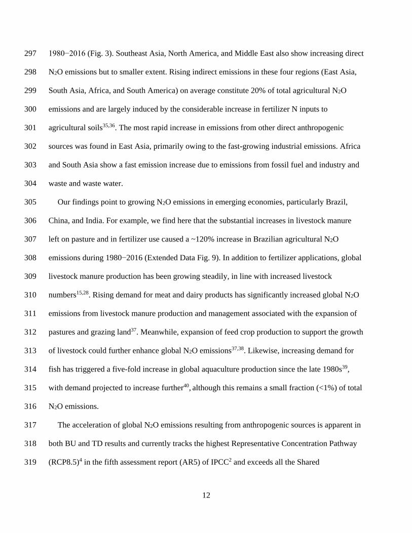
1980−2016 (Fig. 3). Southeast Asia, North America, and Middle East also show increasing direct 297

N2O emissions but to smaller extent. Rising indirect emissions in these four regions (East Asia, 298

South Asia, Africa, and South America) on average constitute 20% of total agricultural N2O 299

emissions and are largely induced by the considerable increase in fertilizer N inputs to 300

agricultural soils35,36. The most rapid increase in emissions from other direct anthropogenic 301

sources was found in East Asia, primarily owing to the fast-growing industrial emissions. Africa 302

and South Asia show a fast emission increase due to emissions from fossil fuel and industry and 303

waste and waste water. 304

Our findings point to growing N2O emissions in emerging economies, particularly Brazil, 305

China, and India. For example, we find here that the substantial increases in livestock manure 306

left on pasture and in fertilizer use caused a ~120% increase in Brazilian agricultural N2O 307

emissions during 1980−2016 (Extended Data Fig. 9). In addition to fertilizer applications, global 308

livestock manure production has been growing steadily, in line with increased livestock 309

numbers15,28. Rising demand for meat and dairy products has significantly increased global N2O 310

emissions from livestock manure production and management associated with the expansion of 311

pastures and grazing land37. Meanwhile, expansion of feed crop production to support the growth 312

of livestock could further enhance global N2O emissions37,38. Likewise, increasing demand for 313

fish has triggered a five-fold increase in global aquaculture production since the late 1980s39, 314

with demand projected to increase further40, although this remains a small fraction (<1%) of total 315

N2O emissions. 316

The acceleration of global N2O emissions resulting from anthropogenic sources is apparent in 317

both BU and TD results and currently tracks the highest Representative Concentration Pathway 318

(RCP8.5)4 in the fifth assessment report (AR5) of IPCC2 and exceeds all the Shared 319

13

Socioeconomic Pathways (SSPs)3 in CMIP6 for the sixth assessment report (AR6) of IPCC (Fig. 320

4). Observed atmospheric N2O concentrations are beginning to exceed predicted levels across all 321

scenarios. Emissions need to be reduced to a level that is consistent with or below that in RCP2.6 322

or SSP1-2.6 in order to limit warming well below the 2° C target of the Paris Agreement. Failure 323

to include N2O within climate mitigation strategies will necessitate even greater abatement of 324

CO2 and CH4. Although N2O mitigation is difficult because N is the key-limiting nutrient in the 325

agricultural production, this study demonstrates that effective mitigation actions have reduced 326

emissions in some regions, such as Europe, through technological improvements in industry and 327

improved N use efficiency in agriculture. 328

There are a number of mitigation options in the agriculture sector available for immediate 329

deployment, including increased N use efficiency in (i) animal production through tuning of feed 330

rations to reduce N excretion, and (ii) in crop production through precision delivery of N 331

fertilizers, split applications and better timing to match N applications to crop demand, 332

conservation tillage, prevention of waterlogging, and the use of nitrification inhibitors43,44. 333

Success stories include the stabilization or reduction of N2O emissions through improving N use 334

efficiency in the United States and Europe, while maintaining or even increasing crop yields44,45. 335

There is every reason to expect that additional implementation of more sustainable practices and 336

emerging technologies will lead to further reductions in these regions. For example, N2O 337

emissions from European agricultural soils decreased by 21% between 1990 and 2010, a decline 338

attributable to the implementation of the Nitrates Directive (an agricultural policy favoring 339

optimization and reduction of fertilizer use as well as water protection legislation)46. For regions 340

where emissions are growing, an immediate opportunity lies in the reduction of excess fertilizer 341

use along with the implementation of more sustainable agricultural practices that together have 342

14

been shown to increase crop yields, reduce N2O emissions, increase water quality, and increase 343

farm income47. In addition, N2O emissions can be efficiently abated in the chemical 344

industry11,43,48,49, as has been achieved successfully in nitric acid plants in the European Union 345

where industrial N2O emissions dropped from 11% to 3% of total emissions between 2007 and 346

2012 (ref. 46). Additional available strategies to reduce N2O emissions include promoting lower 347

meat consumption in some parts of the world9 and reducing food waste11. 348

We present the most comprehensive global N2O budget to date, with a detailed sectorial and 349

regional attribution of sources and sinks. Each of the past four decades had higher global N2O 350

emissions than the previous one, and in all, agricultural activities dominated the growth in 351

emissions. Total industrial emissions have been quite stable with increased emissions from the 352

fossil fuel sector offset to some extent by the decline in emissions in other industrial sectors as a 353

result of successful abatement policies. We also highlight a number of complex interactions 354

between N2O fluxes and human-driven changes whose impact on the global atmospheric N2O 355

growth rate was previously unknown. Those interactions include the effects of climate change, 356

increasing atmospheric CO2, and deforestation. Cumulatively, these exert a relatively small 357

effect on the overall N2O growth, however, individual flux components, such as the growing 358

positive climate-N2O feedback, are significant. These fluxes are not currently included in the 359

national GHG reporting. We further find that Brazil, China, and India dominate the regional 360

contributions to the increase in global N2O emissions over the most recent decade. Our extensive 361

database and modelling capability fill current gaps in national and regional emissions 362

inventories. Future research is needed to further constrain complex biogeochemical interactions 363

between natural/anthropogenic fluxes and global environmental changes, which could lead to 364

significant feedbacks in the future. Reducing excess N applications to croplands and adopting 365

15

precision fertilizer application methods provide the largest immediate opportunities for N2O 366

emissions abatement. 367

368

References 369

1 Prather, M. J. et al. Measuring and modeling the lifetime of nitrous oxide including its 370

variability. Journal of Geophysical Research: Atmospheres 120, 5693-5705 (2015). 371

2 Ciais, P. et al. in Climate Change 2013: The Physical Science Basis. Contribution of 372

Working Group I to the Fifth Assessment Report of the Intergovernmental Panel on 373

Climate Change 465-570 (Cambridge University Press, 2014). 374

3 Gidden, M. J. et al. Global emissions pathways under different socioeconomic scenarios 375

for use in CMIP6: a dataset of harmonized emissions trajectories through the end of the 376

century. Geoscientific Model Development 12, 1443-1475 (2019). 377

4 Davidson, E. A. Representative concentration pathways and mitigation scenarios for 378

nitrous oxide. Environmental Research Letters 7, 024005 (2012). 379

5 Hall, B., Dutton, G. & Elkins, J. The NOAA nitrous oxide standard scale for atmospheric 380

observations. Journal of Geophysical Research: Atmospheres 112, D09305 (2007). 381

6 Prinn, R. G. et al. History of chemically and radiatively important atmospheric gases 382

from the Advanced Global Atmospheric Gases Experiment (AGAGE). Earth System 383

Science Data 10, 985-1018 (2018). 384

7 Butterbach-Bahl, K., Baggs, E. M., Dannenmann, M., Kiese, R. & Zechmeister-385

Boltenstern, S. Nitrous oxide emissions from soils: how well do we understand the 386

processes and their controls? Phil. Trans. R. Soc. B 368, 20130122 (2013). 387

8 Tian, H. et al. The terrestrial biosphere as a net source of greenhouse gases to the 388

atmosphere. Nature 531, 225-228 (2016). 389

9 UNEP. Drawing down N2O to protect climate and the ozone layer. Report No. 390

9280733583, (United Nations Environment Programme (UNEP), 2013). 391

10 Park, S. et al. Trends and seasonal cycles in the isotopic composition of nitrous oxide 392

since 1940. Nature Geoscience 5, 261-265 (2012). 393

11 Davidson, E. A. & Kanter, D. Inventories and scenarios of nitrous oxide emissions. 394

Environmental Research Letters 9, 105012 (2014). 395

12 Reay, D. S. et al. Global agriculture and nitrous oxide emissions. Nature Climate Change 396

2, 410-416 (2012). 397

13 Syakila, A. & Kroeze, C. The global nitrous oxide budget revisited. Greenhouse Gas 398

Measurement and Management 1, 17-26 (2011). 399

14 IPCC. 2006 IPCC Guidelines for National Greenhouse Gas Inventories., (Japan on behalf 400

of the IPCC, Hayama, Japan, 2006). 401

15 Dangal, S. R. et al. Global nitrous oxide emissions from pasturelands and rangelands: 402

Magnitude, spatio‐temporal patterns and attribution. Global Biogeochemical Cycles 33, 403

200-222 (2019). 404

16 Tian, H. Q. et al. Global soil nitrous oxide emissions since the preindustrial era estimated 405

by an ensemble of terrestrial biosphere models: Magnitude, attribution, and uncertainty. 406

Global Change Biology 25, 640-659 (2019). 407

16

17 Wang, Q. et al. Data-driven estimates of global nitrous oxide emissions from croplands. 408

National Science Review 7, 441-452 (2020). 409

18 Thompson, R. L. et al. Acceleration of global N2O emissions seen from two decades of 410

atmospheric inversion. Natural Climate Change 9, 993-998 (2019). 411

19 Zaehle, S., Ciais, P., Friend, A. D. & Prieur, V. Carbon benefits of anthropogenic reactive 412

nitrogen offset by nitrous oxide emissions. Nature Geoscience 4, 601-605 (2011). 413

20 Davidson, E. A. et al. Recuperation of nitrogen cycling in Amazonian forests following 414

agricultural abandonment. Nature 447, 995-998 (2007). 415

21 Verchot, L. V. et al. Land use change and biogeochemical controls of nitrogen oxide 416

emissions from soils in eastern Amazonia. Global Biogeochemical Cycles 13, 31-46 417

(1999). 418

22 Shcherbak, I., Millar, N. & Robertson, G. P. Global metaanalysis of the nonlinear 419

response of soil nitrous oxide (N2O) emissions to fertilizer nitrogen. Proceedings of the 420

National Academy of Sciences 111, 9199-9204 (2014). 421

23 Van Meter, K. J., Basu, N. B., Veenstra, J. J. & Burras, C. L. The nitrogen legacy: 422

emerging evidence of nitrogen accumulation in anthropogenic landscapes. Environmental 423

Research Letters 11, 035014 (2016). 424

24 Firestone, M. K. & Davidson, E. A. Microbiological basis of NO and N2O production and 425

consumption in soil. Exchange of trace gases between terrestrial ecosystems the 426

atmosphere 47, 7-21 (1989). 427

25 Griffis, T. J. et al. Nitrous oxide emissions are enhanced in a warmer and wetter world. 428

Proceedings of the National Academy of Sciences 114, 12081-12085 (2017). 429

26 Pärn, J. et al. Nitrogen-rich organic soils under warm well-drained conditions are global 430

nitrous oxide emission hotspots. Nature Communications 9, 1135 (2018). 431

27 Smith, K. The potential for feedback effects induced by global warming on emissions of 432

nitrous oxide by soils. Global Change Biology 3, 327-338 (1997). 433

28 FAOSTAT. The Food and Agriculture Organization of the United Nations Statistics: 434

Emissions-Agriculture, Emissions Land Use Trade (Crops and livestock products), 435

Population, Agri-Environmental Indicators (Livestock Manure) (2019). 436

29 Xu, R. et al. Increased nitrogen enrichment and shifted patterns in the world's grassland: 437

1860–2016. Earth System Science Data 11, 175-187 (2019). 438

30 Beusen, A. H., Bouwman, A. F., Van Beek, L. P., Mogollón, J. M. & Middelburg, J. J. 439

Global riverine N and P transport to ocean increased during the 20th century despite 440

increased retention along the aquatic continuum. Biogeosciences 13, 2441-2451 (2016). 441

31 MacLeod, M., Hasan, M. R., Robb, D. H. F. & Mamun-Ur-Rashid, M. Quantifying and 442

mitigating greenhouse gas emissions from global aquaculture. FAO, Rome (2019). 443

32 Buitenhuis, E. T., Suntharalingam, P. & Le Quéré, C. Constraints on global oceanic 444

emissions of N2O from observations and models. Biogeosciences 15, 2161-2175 (2018). 445

33 Manizza, M., Keeling, R. F. & Nevison, C. D. On the processes controlling the seasonal 446

cycles of the air–sea fluxes of O2 and N2O: A modelling study. Tellus B: Chemical and 447

Physical Meteorology 64, 18429 (2012). 448

34 Martinez-Rey, J., Bopp, L., Gehlen, M., Tagliabue, A. & Gruber, N. Projections of 449

oceanic N2O emissions in the 21st century using the IPSL Earth system model. 450

Biogeosciences 12, 4133-4148 (2015). 451

35 Maavara, T. et al. Nitrous oxide emissions from inland waters: Are IPCC estimates too 452

high? Global Change Biology 25, 473-488 (2019). 453

17

36 Yao, Y. et al. Increased global nitrous oxide emissions from streams and rivers in the 454

Anthropocene. Natural Climate Change 10, 138-142 (2020). 455

37 Gerber, P. J. et al. Tackling climate change through livestock: a global assessment of 456

emissions and mitigation opportunities. FAO (2013). 457

38 Herrero, M. et al. Biomass use, production, feed efficiencies, and greenhouse gas 458

emissions from global livestock systems. Proceedings of the National Academy of 459

Sciences 110, 20888-20893 (2013). 460

39 Yuan, J. et al. Rapid growth in greenhouse gas emissions from the adoption of industrial-461

scale aquaculture. Nature Climate Change 9, 318-322 (2019). 462

40 Froehlich, H. E., Runge, C. A., Gentry, R. R., Gaines, S. D. & Halpern, B. S. 463

Comparative terrestrial feed and land use of an aquaculture-dominant world. Proceedings 464

of the National Academy of Sciences 115, 5295-5300 (2018). 465

41 O'Neill, B. C. et al. The Scenario Model Intercomparison Project (ScenarioMIP) for 466

CMIP6. Geoscience Model Development 9, 3461-3482 (2016). 467

42 Gütschow, J. et al. The PRIMAP-hist national historical emissions time series. Earth 468

System Science Data 8, 571-603 (2016). 469

43 Winiwarter, W., Höglund-Isaksson, L., Klimont, Z., Schöpp, W. & Amann, M. Technical 470

opportunities to reduce global anthropogenic emissions of nitrous oxide. Environmental 471

Research Letters 13, 014011 (2018). 472

44 Zhang, X. et al. Managing nitrogen for sustainable development. Nature 528, 51-59 473

(2015). 474

45 Mueller, N. D. et al. Declining spatial efficiency of global cropland nitrogen allocation. 475

Global Biogeochemical Cycles 31, 245-257 (2017). 476

46 European Environment Agency. Annual European Union greenhouse gas inventory 1990‐477

2017 and inventory report 2019. Submission under the United Nations Framework 478

Convention on Climate Change and the Kyoto Protocol, Copenhagen, DK (2019). 479

47 Cui, Z. et al. Pursuing sustainable productivity with millions of smallholder farmers. 480

Nature 555, 363-366 (2018). 481

48 Kanter, D. et al. A post-Kyoto partner: considering the stratospheric ozone regime as a 482

tool to manage nitrous oxide. Proceedings of the National Academy of Sciences 110, 483

4451-4457 (2013). 484

49 Schneider, L., Lazarus, M. & Kollmuss, A. J. S. M. S. E. I. Industrial N2O projects under 485

the CDM: Adipic acid-A case of carbon leakage. Stockholm Environment Institute 486

(2010). 487

488

489

490

491

492

493

494

495

18

Table 1 The global N2O budget in the 1980s, 1990s, 2000s, and 2007−2016. 496

the 1980s the 1990s the 2000s 2007-2016

Anthropogenic sources mean min max mean min max mean min max mean min max

Direct emissions of N additions in the agricultural

sector (Agriculture)

Direct soil emissions 1.5 0.9 2.6 1.7 1.1 3.1 2.0 1.3 3.4 2.3 1.4 3.8

Manure left on pasture 0.9 0.7 1.0 1.0 0.7 1.1 1.1 0.8 1.2 1.2 0.9 1.3

Manure management 0.3 0.2 0.4 0.3 0.2 0.4 0.3 0.2 0.5 0.3 0.2 0.5

Aquaculture 0.01 0.00 0.03 0.03 0.01 0.1 0.1 0.02 0.2 0.1 0.02 0.2

sub-total 2.6 1.8 4.1 3.0 2.1 4.8 3.4 2.3 5.2 3.8 2.5 5.8

Other direct anthropogenic

sources

Fossil fuel and industry 0.9 0.8 1.1 0.9 0.9 1.0 0.9 0.8 1.0 1.0 0.8 1.1

Waste and waste water 0.2 0.1 0.3 0.3 0.2 0.4 0.3 0.2 0.4 0.3 0.2 0.5

Biomass burning 0.7 0.7 0.7 0.7 0.6 0.8 0.6 0.6 0.6 0.6 0.5 0.8

sub-total 1.8 1.6 2.1 1.9 1.7 2.1 1.8 1.6 2.1 1.9 1.6 2.3

Indirect emissions from

anthropogenic N additions

Inland waters, estuaries, coastal zones

0.4 0.2 0.5 0.4 0.2 0.5 0.4 0.2 0.6 0.5 0.2 0.7

Atmospheric N deposition on land

0.6 0.3 1.2 0.7 0.4 1.4 0.7 0.4 1.3 0.8 0.4 1.4

Atmospheric N deposition on ocean

0.1 0.1 0.2 0.1 0.1 0.2 0.1 0.1 0.2 0.1 0.1 0.2

sub-total 1.1 0.6 1.9 1.2 0.7 2.1 1.2 0.6 2.1 1.3 0.7 2.2

Perturbed fluxes from

climate/CO2/land cover change

CO2 effect -0.2 -0.3 0.0 -0.2 -0.4 0.0 -0.3 -0.5 0.1 -0.3 -0.6 0.1

Climate effect 0.4 0.0 0.8 0.5 0.1 0.9 0.7 0.3 1.2 0.8 0.3 1.3

Post-deforestation pulse effect

0.7 0.6 0.8 0.7 0.6 0.8 0.7 0.7 0.8 0.8 0.7 0.8

Long-term effect of reduced mature forest area

-0.8 -0.8 -0.9 -0.9 -0.8 -1.0 -1.0 -0.9 -1.1 -1.1 -1.0 -1.1

sub-total 0.1 -0.4 0.7 0.1 -0.5 0.7 0.2 -0.4 0.9 0.2 -0.6 1.1

Anthropogenic total 5.6 3.6 8.7 6.2 3.9 9.7 6.7 4.1 10.3 7.3 4.2 11.4

Natural fluxes

Natural soils baseline 5.6 4.9 6.6 5.6 4.9 6.5 5.6 5.0 6.5 5.6 4.9 6.5

Ocean baseline 3.6 3.0 4.4 3.5 2.8 4.4 3.5 2.7 4.3 3.4 2.5 4.3

Natural (Inland waters, estuaries, coastal zones)

0.3 0.3 0.4 0.3 0.3 0.4 0.3 0.3 0.4 0.3 0.3 0.4

Lightning and atmospheric production 0.4 0.2 1.2 0.4 0.2 1.2 0.4 0.2 1.2 0.4 0.2 1.2

Surface sink -0.01 0.00 -0.3 -0.01 0.00 -0.3 -0.01 0.00 -0.3 -0.01 0.00 -0.3

Natural total 9.9 8.5 12.2 9.8 8.3 12.1 9.8 8.2 12.0 9.7 8.0 12.0

Bottom-up total source

15.5 12.1 20.9 15.9 12.2 21.7 16.4 12.3 22.4 17.0 12.2 23.5

Top-down Ocean 5.1 3.1 7.2 5.1 3.4 7.1

Top-down Land 10.8 9.3 12.5 11.8 10.6 13.8

Top-down total source

15.9 15.1 16.9 16.9 15.9 17.7

Top-down Statospheric sink 12.1 11.4 13.1 12.4 11.7 13.3

Observed atmospheric chemical sink* 13.3 12.2 14.4 13.5 12.4 14.6

Change in atmospheric abundance** 3.7 3.2 4.2 4.3 3.8 4.8

Atmospheric burden

1462 1442 1482 1493 1472 1514 1531 1510 1552 1555 1533 1577

Note: BU estimates include four categories of anthropogenic sources (red for agriculture, orange for 497 other direct anthropogenic sources, maroon for indirect emissions from anthropogenic N additions, and 498 brown for perturbed fluxes from climate/CO2/land cover change) and one category for natural sources 499 and sinks (green). The sources and sinks of N2O are given in Tg N yr-1. The atmospheric burden is given 500 in Tg N. *calculated from satellite observations with a photolysis model (about 1% of this sink 501 occurs in the troposphere). **Calculated from the combined NOAA and AGAGE record of surface N2O, 502 and adopting the uncertainty of the IPCC AR5 (Chapter 6)2. Detailed information on calculating each 503 sub-category is shown in Supplementary Tables 1−13. 504

19

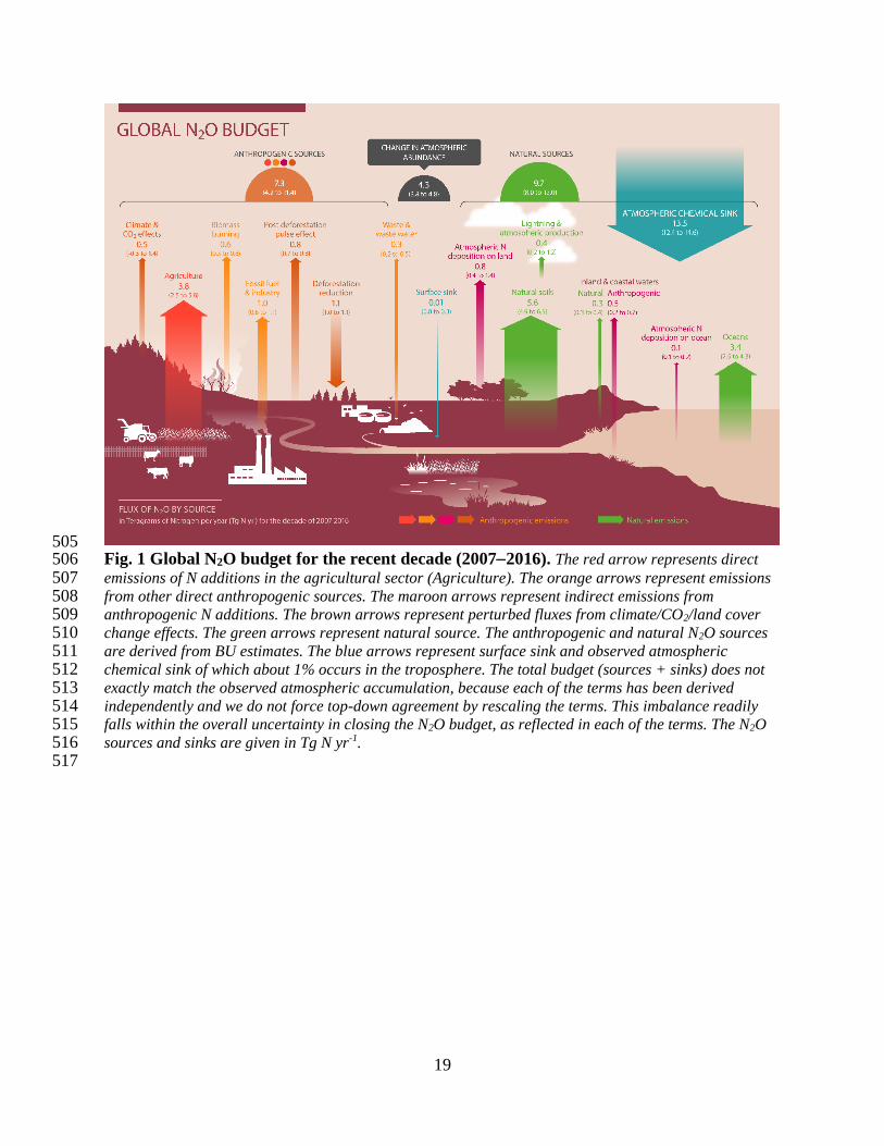
505 Fig. 1 Global N2O budget for the recent decade (2007−2016). The red arrow represents direct 506 emissions of N additions in the agricultural sector (Agriculture). The orange arrows represent emissions 507 from other direct anthropogenic sources. The maroon arrows represent indirect emissions from 508 anthropogenic N additions. The brown arrows represent perturbed fluxes from climate/CO2/land cover 509 change effects. The green arrows represent natural source. The anthropogenic and natural N2O sources 510 are derived from BU estimates. The blue arrows represent surface sink and observed atmospheric 511 chemical sink of which about 1% occurs in the troposphere. The total budget (sources + sinks) does not 512 exactly match the observed atmospheric accumulation, because each of the terms has been derived 513 independently and we do not force top-down agreement by rescaling the terms. This imbalance readily 514 falls within the overall uncertainty in closing the N2O budget, as reflected in each of the terms. The N2O 515 sources and sinks are given in Tg N yr-1. 516 517

20

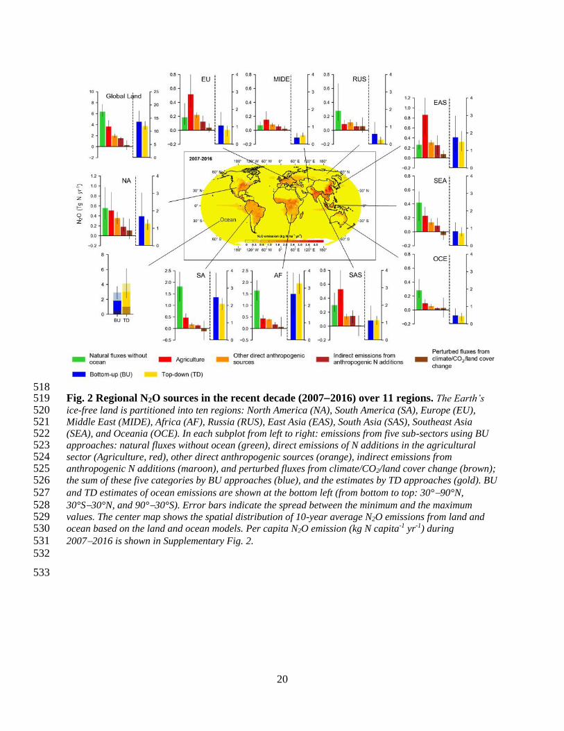
518 Fig. 2 Regional N2O sources in the recent decade (2007−2016) over 11 regions. The Earth’s 519 ice-free land is partitioned into ten regions: North America (NA), South America (SA), Europe (EU), 520 Middle East (MIDE), Africa (AF), Russia (RUS), East Asia (EAS), South Asia (SAS), Southeast Asia 521 (SEA), and Oceania (OCE). In each subplot from left to right: emissions from five sub-sectors using BU 522 approaches: natural fluxes without ocean (green), direct emissions of N additions in the agricultural 523 sector (Agriculture, red), other direct anthropogenic sources (orange), indirect emissions from 524 anthropogenic N additions (maroon), and perturbed fluxes from climate/CO2/land cover change (brown); 525 the sum of these five categories by BU approaches (blue), and the estimates by TD approaches (gold). BU 526 and TD estimates of ocean emissions are shown at the bottom left (from bottom to top: 30°−90°N, 527 30°S−30°N, and 90°−30°S). Error bars indicate the spread between the minimum and the maximum 528 values. The center map shows the spatial distribution of 10-year average N2O emissions from land and 529 ocean based on the land and ocean models. Per capita N2O emission (kg N capita-1 yr-1) during 530 2007−2016 is shown in Supplementary Fig. 2. 531 532

533

21

534 Fig. 3 Ensembles of regional anthropogenic N2O emissions over the 1980−2016 period. The 535 bar chart in the center shows the accumulated changes in regional and global N2O emissions during the 536 study period. Error bars indicate the 95% confidence interval for the average of accumulated changes. 537 The Mann-Kendall test was performed to examine a monotonic increasing or decreasing trend in the 538 estimated ensemble N2O emissions for each region and the globe during 1980−2016. The accumulated 539 changes were calculated from the linear regressed annual change rate (Tg N yr-2) multiplied by 37 years. 540 All regions except SEA show a significant increasing or decreasing trend in the estimated ensemble N2O 541 emissions during the study period (indicated by for each bar). 542 543

544

22

545 Fig. 4 Historical and projected global anthropogenic N2O emissions and concentrations. 546

Global anthropogenic N2O emissions (a, b) and concentrations (c, d) compared to the four 547

representative concentration pathways (RCPs) in the IPCC AR5 (a, c, ref. 2) and the new marker 548

scenarios based on the Shared Socioeconomic Pathways (SSPs) used in CMIP6 (b, d, ref. 41). 549

The historical data is represented as the mean of the BU and TD estimates of anthropogenic N2O 550

emissions, while the atmospheric concentration uses the three observation networks available, 551

AGAGE, NOAA, and CSIRO. TD anthropogenic emissions were calculated by subtracting BU-552

derived natural fluxes. To aid the comparison, the four RCPs were shifted down so that the 2005 553

value is equal to the 2000−2009 average of the mean of TD and BU estimates. The SSPs are 554

harmonized3 to match the historical emissions used in CMIP642 and Extended Data Fig. 10 555

shows the unharmonized data. 556

557

558

559

23

Methods 560

Terminology. This study provides an estimation of the global N2O budget considering all 561

possible sources and all global change processes that can perturb the budget. A total of 18 562

sources and three sinks of N2O are identified and grouped into six categories (Figure 1, Table 1): 563

1) Natural fluxes in absence of climate change and anthropogenic disturbances including Soil 564

emissions, Surface sink, Ocean emissions, Lightning and atmospheric production, and Natural 565

emission from inland waters, estuaries, coastal zones (inland and coastal waters), 2) Perturbed 566

fluxes from climate/CO2/land cover change including CO2 effect, Climate effect, Post-567

deforestation pulse effect, and Long-term effect of reduced mature forest area, 3) Direct 568

emissions of N additions in the agricultural sector (Agriculture) including emissions from direct 569

application of synthetic N fertilizers and manure (henceforth Direct soil emissions), Manure left 570

on pasture, Manure management, and Aquaculture, 4) Indirect emissions from anthropogenic N 571

additions including atmospheric N deposition (NDEP) on land, atmospheric NDEP on ocean, and 572

effects of anthropogenic loads of reactive N in inland waters, estuaries, coastal zones, 5) Other 573

direct anthropogenic sources including Fossil fuel and industry, Waste and waste water, and 574

Biomass burning, and 6) Two estimates of stratospheric sinks obtained from atmospheric 575

chemistry transport models and observations, and one tropospheric sink (Table 1, Extended Data 576

Fig. 2). 577

For the purpose of compiling national GHG inventories for country reporting to the climate 578

convention, our anthropogenic N2O emission categories are aligned with those used in UNFCCC 579

reporting and IPCC 2006 methodologies (Supplementary Table 14). We also provide the detailed 580

comparison of our methodology and quantification with the IPCC AR5 (see Supplementary 581

Section 4; Supplementary Table 15). 582

24

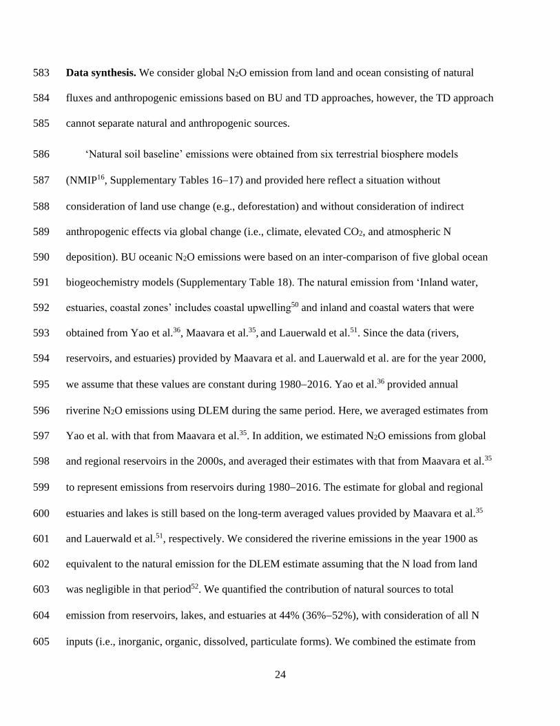
Data synthesis. We consider global N2O emission from land and ocean consisting of natural 583

fluxes and anthropogenic emissions based on BU and TD approaches, however, the TD approach 584

cannot separate natural and anthropogenic sources. 585

‘Natural soil baseline’ emissions were obtained from six terrestrial biosphere models 586

(NMIP16, Supplementary Tables 16−17) and provided here reflect a situation without 587

consideration of land use change (e.g., deforestation) and without consideration of indirect 588

anthropogenic effects via global change (i.e., climate, elevated CO2, and atmospheric N 589

deposition). BU oceanic N2O emissions were based on an inter-comparison of five global ocean 590

biogeochemistry models (Supplementary Table 18). The natural emission from ‘Inland water, 591

estuaries, coastal zones’ includes coastal upwelling50 and inland and coastal waters that were 592

obtained from Yao et al.36, Maavara et al.35, and Lauerwald et al.51. Since the data (rivers, 593

reservoirs, and estuaries) provided by Maavara et al. and Lauerwald et al. are for the year 2000, 594

we assume that these values are constant during 1980−2016. Yao et al.36 provided annual 595

riverine N2O emissions using DLEM during the same period. Here, we averaged estimates from 596

Yao et al. with that from Maavara et al.35. In addition, we estimated N2O emissions from global 597

and regional reservoirs in the 2000s, and averaged their estimates with that from Maavara et al.35 598

to represent emissions from reservoirs during 1980−2016. The estimate for global and regional 599

estuaries and lakes is still based on the long-term averaged values provided by Maavara et al.35 600

and Lauerwald et al.51, respectively. We considered the riverine emissions in the year 1900 as 601

equivalent to the natural emission for the DLEM estimate assuming that the N load from land 602

was negligible in that period52. We quantified the contribution of natural sources to total 603

emission from reservoirs, lakes, and estuaries at 44% (36%−52%), with consideration of all N 604

inputs (i.e., inorganic, organic, dissolved, particulate forms). We combined the estimate from 605

25

lightning with that from atmospheric production into an integrated category ‘Lightning and 606

atmospheric production’. We make the simplification of considering the category ‘Lightning and 607

atmospheric production’ as purely natural, however, atmospheric production is affected to some 608

extent by anthropogenic activities through enhancing the concentrations of the reactive species 609

NH2 and NO2. This category is in any case very small and the anthropogenic enhancement effect 610

is uncertain. Lightning produces NOx, the median estimate of which is 5 Tg N yr-1 (ref. 53). We 611

assumed an EF of 1% (ref. 54) and a global estimate of 0.05 (0.02−0.09) Tg N yr-1 from lightning. 612

Atmospheric production of N2O results from the reaction of NH2 with NO2 (refs. 55,56), N with 613

NO2, and oxidation of N2 by O(1D)57, all of which constitute an estimated source of 0.3 (0.2−1.1) 614

Tg N yr-1. The estimate of ‘Surface sink’ was obtained from Schlesinger58 and Syakila et al.59. 615

The anthropogenic sources include four sub-sectors: 616

(a) Agriculture. It consists of four components: ‘Direct soil emissions’, ‘Manure left on 617

pasture’, ‘Manure management’, and ‘Aquaculture’. Data for ‘Direct soil emissions’ were 618

obtained as the ensemble mean of N2O emissions from an average of three inventories (EDGAR 619

v4.3.2, FAOSTAT, and GAINS), the SRNM/DLEM models, and the NMIP/DLEM models. The 620

statistical model SRNM only covers cropland N2O emissions, the same as the NMIP. Thus, we 621

add the DLEM-based estimate of pasture N2O emissions into the two estimates in cropland to 622

represent direct agricultural soil emissions (i.e., SRNM/DLEM or NMIP/DLEM). The ‘Manure 623

left on pasture’ and ‘Manure management’ emissions are the ensemble mean of EDGAR v4.3.2, 624

FAOSTAT, and GAINS databases. Global N flows (i.e., fish feed intake, fish harvest, and waste) 625

in freshwater and marine aquaculture were obtained from Beusen et al.30 and Bouwman et al.60,61 626

based on a nutrient budget model for the period 1980−2016. We then calculated global 627

aquaculture N2O emissions through considering 1.8% loss of N waste in aquaculture, the same 628

26

EF used in Hu et al.62 and Macleod et al.31. The uncertainty range of the EF is from 0.5% (ref. 14) 629

to 5% (ref. 63), the same range used in the UNEP report9. The ‘Aquaculture’ emission for the 630

period 2007−2016 was a synthesis data from Hu et al.62 in 2009, the FAO Report31 in 2013, and 631

our calculations. The estimate of aquaculture N2O emission prior to 2009 was from our 632

calculations only. 633

The estimated direct emissions from agriculture have increased from 2.6 (1.8−4.1) Tg N yr-1 634

in the 1980s to 3.8 (2.5−5.8) Tg N yr-1 over the recent decade (2007−2016, Table 1). 635

Specifically, direct soil emission from the application of fertilizers is the major source and 636

increased at a rate of 0.27±0.01 Tg N yr-1 per decade (P < 0.05; Table 1). Compared with the 637

three global inventories (FAOSTAT, EDGAR v4.3.2, and GAINS), the estimates from process-638

based models (NMIP/DLEM15,16) and a statistical model (SRNM)/DLEM15,17 exhibited a faster 639

increase (Extended Data Fig. 4a). Over the past four decades, we also found a small but 640

significant increase in emissions from livestock manure (i.e., manure left on pasture and manure 641

management) at a rate of 0.1±0.01 Tg N yr-1 per decade (P < 0.05; Extended Data Fig. 4b-c). 642

Meanwhile, global aquaculture N2O emissions increased 10-fold, however, this flux remains the 643

smallest term in the global budget (Extended Data Fig. 4d). 644

(b) Other direct anthropogenic sources. It includes ‘Fossil fuel and industry’, ‘Waste and 645

waste water’, and ‘Biomass burning’. Both ‘Fossil fuel and industry’ and ‘Waste and waste 646

water’ are the ensemble means of EDGAR v4.3.2 and GAINS databases. The ‘Biomass burning’ 647

emission is the ensemble mean of FAOSTAT, DLEM, and GFED4s databases. 648

Emissions from a combination of fossil fuel and industry, waste and waste water, and biomass 649

burning increased from 1.8 (1.6−2.1) Tg N yr-1 in the 1980s to 1.9 (1.6−2.3) Tg N yr-1 over the 650

period of 2007−2016 (Table 1). The waste and waste water emission showed a continuous 651

27

increase at a rate of 0.04±0.01 Tg N yr-1 per decade (P < 0.05) (Extended Data Fig. 5c). 652

Emissions from biomass burning, estimated based on three data sources (DLEM, GFED4s, and 653

FAOSTAT), slightly decreased at a rate of -0.03±0.04 Tg N yr-1 per decade (P = 0.3) since 654

the1980s (Extended Data Fig. 5d). This item is largely affected by climate and land use 655

change64,65. Of the three data sources, the DLEM estimate exhibited significant inter-annual 656

variability, especially during 1980−2000 when extreme fire events were detected in 1982, 1987, 657

1991, 1994, and 1998. The occurrences of these extreme fires were associated with El Niño-658

Southern Oscillation (ENSO) events, especially in Indonesia (e.g., ‘Great Fire of Borneo’ in 659

1982) 66. Since 1997, N2O emissions from fires estimated by DLEM, GFED4s, and FAOSTAT 660

were consistent in the inter-annual variability. All the three estimates showed a decreasing trend, 661

agreeing well with satellite-observed decrease of global burned area64,65. 662

(c) Indirect emissions from anthropogenic N additions. Data were obtained from various 663

sources and considered N deposition on land and ocean (‘N deposition on land’ and ‘N 664

deposition on ocean’), as well as the N leaching and runoff from upstream (‘Inland and coastal 665

waters’). The emission from ‘N deposition on ocean’ was provided by Suntharalingam et al.67, 666

while emission from ‘N deposition on land’ was the ensemble mean of an average of three 667

inventories: FAOSTAT/EDGAR v4.3.2, GAINS/EDGAR v4.3.2, and NMIP. FAOSTAT and 668

GAINS documented the sector ‘Indirect agricultural N2O emissions’ by separating estimates 669

from N leaching or N deposition, while EDGAR v4.3.2 did not. Here, we treated ‘Indirect 670

agricultural N2O emissions’ from EDGAR v4.3.2 as ‘Inland and coastal waters’ emissions for 671

data synthesis. Only EDGAR v4.3.2 provided an estimate of indirect emission from non-672

agricultural sectors, while both FAOSTAT and GAINS, following the IPCC guidelines, provided 673

NHx/NOy volatilization from agricultural sectors. Here, we sum FAOSTAT or GAINS with 674

28

EDGAR v4.3.2 (i.e., FAOSTAT/EDGAR v4.3.2 or GAINS/EDGAR v4.3.2) to represent N 675

deposition induced soil emissions from both agricultural and non-agricultural sectors. The N2O 676

emissions from ‘Inland and coastal waters’ consist of rivers, reservoirs, lakes, estuaries, and 677

coastal zone, which is the ensemble mean of an average of three inventories (EDGAR v4.3.2, 678

FAOSTAT, GAINS), and the mean of process-based models. The anthropogenic emission 679

estimated by Yao et al.36 considered annual N inputs and other environmental factors (i.e., 680

climate, elevated CO2, and land cover change). For long-term average in rivers, reservoirs, 681

estuaries and lakes, we applied a mean of 56% (based on the ratio of anthropogenic to total N 682

additions from land) to calculate anthropogenic emissions. Seagrass, mangrove, saltmarsh and 683

intertidal N2O emissions were undated from Murray et al68. Coastal waters with low disturbance 684

generally either have low N2O emissions or act as a sink for N2O69,70. Here, coastal zone 685

emissions were treated as anthropogenic emissions due to intensive human disturbances71. 686

N2O emissions following transport of anthropogenic N additions via atmosphere and water 687

bodies increased from 1.1 (0.6−1.9) Tg N yr-1 in the 1980s to 1.3 (0.7−2.2) Tg N yr-1 during 688

2007−2016 (Table 1). The N2O emissions from inland and coastal waters increased at a rate of 689

0.03±0.00 Tg N yr-1 per decade (P < 0.05). Such an increase was reported by all the three 690

inventories (FAOSTAT, GAINS, and EDGAR v4.3.2) with FAOSTAT giving the largest 691

estimate. In contrast, the DLEM-based estimate presented a divergent trend: first increasing from 692

1980−1998 and then slightly decreasing thereafter (Extended Data Fig. 6a). Emissions from 693

atmospheric N deposition on oceans were relatively constant with a value of 0.1 (0.1−0.2) Tg N 694

yr-1, while a large increase in emissions was found from atmospheric N deposition on land, with 695

0.06±0.01 Tg N yr-1 per decade (P < 0.05) reported in the three estimates (FAOSTAT/EDGAR 696

v4.3.2, GAINS/EDGAR v4.3.2, and NMIP). The FAOSTAT agricultural source, together with 697

29

the EDGAR v4.3.2 industrial source, is consistent with NMIP estimates in the magnitude of N2O 698

emissions, with the latter estimating a slightly slower increase from 2010 to 2016 (Extended 699

Data Fig. 6b). 700

(d) Perturbed fluxes from climate/CO2/land cover change. Perturbed N2O fluxes represent the 701

sum of the effects of climate, elevated atmospheric CO2, and land cover change. The estimate of 702

climate and CO2 effects on emissions was based on NMIP. The effect of land cover change on 703

N2O dynamics includes the reduction due to ‘Long-term effect of reduced mature forest area’ 704

and the emissions due to ‘Post-deforestation pulse effect’. The two estimates were based on the 705

book-keeping approach and the DLEM model simulation. The book-keeping method is 706

developed by Houghton et al.72 for accounting for carbon flows due to land use. In this study, an 707

observation dataset consisting of 18 tropical sites was collected to follow the book-keeping logic. 708

The dataset covers N2O emissions from a reference mature forest and their nearby converted 709

pastures aged between one and 60 years. The average tropical forest N2O emission rate of 1.974 710

kg N2O-N ha-1 yr-1 was adopted as the baseline73. Two logarithmic response curves of soil N2O 711

emissions (normalized to the baseline) after deforestation were developed: 𝑦 = −0.31 𝑙𝑛( 𝑥) +712

1.53 (𝑅2 = 0.30) and 𝑦 = −0.454 𝑙𝑛( 𝑥) + 2.21 (𝑅2 = 0.09). The first logarithmic function 713

uses data collected by a review analysis74, based upon which the second one further considers 714

observations from Verchot et al.21 and Keller and Reiners75. In the first function, x (unit: year) 715

indicates pasture age in years after deforestation and y (unitless; 0−1) indicates the ratio of 716

pasture N2O emission over the N2O emission from the nearby reference mature forest. In the 717

second function, x (unit: year) indicates secondary forest age and y (unitless; 0−1) indicates the 718

ratio of secondary forest N2O emission over that of a reference mature forest. This form of the 719

response functions can effectively reproduce the short-lived increase in soil N2O emissions after 720

30

initial forest clearing and the gradually declining emission rates of converted crops/pastures21,76. 721

Using these two curves and the baseline, we kept track of the N2O reduction of tropical forests 722

and the post-deforestation crop/pasture N2O emissions at an annual time-scale. This book-723

keeping method was applied to the two deforestation area datasets (Supplementary Text 2.8), so 724

we could investigate not only the difference caused by the two sets of land use data but also the 725

difference between this empirical method and the process-based model. For land conversion 726

from natural vegetation to croplands or pastures, DLEM uses a similar strategy to Houghton et 727

al.72 and McGuire et al.77 to simulate its influences on carbon and N cycles. Moreover, through 728

using the sites of field observation from Davidson et al.20 and Keller and Reiners75, we estimated 729

N2O emission from secondary tropical forests based on the algorithm: y = 0.0084x + 0.2401 (R2 730

= 0.44). x (unit: year) indicates secondary forest age and y (unitless; 0−1) indicates the ratio of 731

secondary forest N2O emission over that of a reference mature forest. The difference between 732

primary forests and secondary forests were subtracted from natural soil emissions simulated by 733

six terrestrial biosphere models in NMIP. 734

We calculated the ensemble of oceanic N2O emission based on the BU approach (five ocean 735

biogeochemical models; Supplementary Table 18) and the TD approach (five estimates from 736

four inversion models; Supplementary Table 19), respectively. The atmospheric burden and its 737

rate of change during 1980−2016 were derived from mean maritime surface mixing ratios of 738

N2O (refs. 78,79) with a conversion factor of 4.79 Tg N/ppb (ref. 80). Combining uncertainties in 739

measuring the mean surface mixing ratios78 and that of converting surface mixing ratios to a 740

global mean abundance80, we estimate a ±1.4% uncertainty in the burden. Annual change in 741

atmospheric abundance is calculated from the combined NOAA and AGAGE record of surface 742

N2O and uncertainty is taken from the IPCC AR5 (ref. 2). There shows an agreement of the 743

31

stratospheric loss from atmospheric chemistry transport models (TD modeled chemical sink18,81) 744

and from satellite observations with a photolysis model (observed photochemical sink1), which 745

differ only by ~1 Tg N yr-1. The satellite-based lifetime, 116±9 years, gives an overall 746

uncertainty in the annual loss of ±8%. The tropospheric loss of N2O from reaction with O(1D) is 747

included in observed atmospheric chemical sink (Table 1) and is small (~1% of the stratospheric 748

sink) with an estimated range of 0.1 to 0.2 Tg N yr-1. 749

Comparison with the IPCC guidelines. The IPCC has provided guidance to quantify N2O 750

emissions, which is widely used in emission inventories for reporting to the UNFCCC. Over time 751

the recommended approaches have changed, which is critical for estimating emissions from 752

agricultural soils, the largest emission source. Previous global N2O assessments52,82,83 based on 753

the IPCC 1996 guidelines84 attributed about 6.3 Tg N yr-1 to the agricultural sector, including 754

both direct and indirect emissions. This estimate is significantly larger than our results (Fig. 1; 755

Table 1) derived from multiple methods, and is also larger than the most recent estimates from 756

global inventories (EDGAR v4.3.2, FAOSTAT, and GAINS) that are based on the IPCC 2006 757

guidelines14. The main reason is that indirect emissions from leaching and groundwater were 758

overestimated in previous studies85. Correspondingly, projections of atmospheric N2O 759

concentrations based on these overestimated emissions82 led to biased estimates. For example, 760

Mosier and Kroeze82 expected atmospheric N2O concentrations to be 340−350 ppb in the year 761

2020, instead of 333 ppb5 as observed. Recently, the 2019 Refinement to the 2006 IPCC 762

Guidelines for National Greenhouse Gas Inventories has been published. It adopts the same 763

approach for N application on soils, but considers impacts of different climate regimes. The new 764

guidelines, based on a wealth of new scientific literature, proposed much smaller emissions from 765

grazing animals by a factor of 5−7. Preliminary calculations we have made indicate that global 766

32

soil emissions based on these new guidelines may decrease by 20%−25%. Integrating estimates 767

relying on the IPCC methodology with estimates by process-based models provides for a more 768

balanced assessment in this paper. We also added information from assessments86,87 that derived 769

agricultural emissions as the difference between atmospheric terms and other emissions like 770

combustion, industry and nature, and they gave comparable magnitudes (4.3−5.8 Tg N yr-1) to 771

our bottom-up results. 772

Uncertainty. Current data analysis and synthesis of long-term N2O fluxes are based on a wide 773

variety of TD and BU methods. TD approaches, consisting of four inversion frameworks88-91, 774

provide a wide range of estimates largely due to systematic errors in the modelled atmospheric 775

transport and stratospheric loss of N2O. In addition, the emissions from TD analyses are 776

dependent on the magnitude and distribution of the prior flux estimates to an extent that is 777

strongly determined by the number of atmospheric N2O measurements18. Inversions are 778

generally not well constrained (and thus rely heavily on a priori estimates) in Africa, Southeast 779

Asia, southern South America, and over the oceans, owing to the paucity of observations in these 780

regions. The improvement of atmospheric transport models, more accurate priors, and more 781

atmospheric N2O measurements would reduce uncertainty in further TD estimates, particularly 782

for ocean and regional emissions. 783

BU approaches are subject to uncertainties in various sources from land16 and oceans32. For 784

process-based models (e.g. NMIP and ocean biogeochemical models), the uncertainty is 785

associated with differences in model configuration as well as process parameterization16,32. The 786

uncertainty of estimates from NMIP could be reduced in multiple ways16. First, the six models in 787

NMIP exhibited different spatial and temporal patterns of N2O emissions even though they used 788

the same forcings. Although these models have considered essential biogeochemical processes in 789

33

soils (e.g., biological N fixation, nitrification/denitrification, mineralization/immobilization, 790

etc.)92, some missing processes such as freeze-thaw cycles and ecosystem disturbances should be 791

included in terrestrial biosphere models to reduce uncertainties. Second, the quality of input 792

datasets, specifically the amount and timing of N application, and spatial and temporal changes 793

in distribution of natural vegetation and agricultural land, is critical for accurately simulating soil 794

N2O emissions. Third, national and global N2O flux measurement networks17 could be used to 795

validate model performance and constrain large-scale model simulations. Data assimilation 796

techniques could be utilized to improve model accuracy. 797

Current remaining uncertainty in global ocean model estimates of N2O emission includes the 798

contribution of N2O flux derived from the tropical oceanic low oxygen zones (e.g., the Eastern 799

Equatorial Pacific, the northern Indian ocean) relative to the global ocean. These low oxygen 800

zones are predominantly influenced by high yield N2O formation processes (e.g., denitrification 801

and enhanced nitrification). Regional observation-based assessments have also suggested that 802

these regions may produce more N2O than is simulated by the models32. The current generation 803

of global ocean biogeochemistry models are not sufficiently accurate to represent the high N2O 804

production processes in low-oxygen zones, and their associated variability (see refs. 34,93,94 for 805

more detail). Thus, precisely representing the local ocean circulation and associated 806

biogeochemical fluxes of these regions could further reduce the uncertainty in estimates of 807

global and regional oceanic N2O emissions. 808

Regardless of the tier approach used, GHG inventories for agriculture suffer from high 809

uncertainty in the underlying agriculture and rural data and statistics used as input, including 810

statistics on fertilizer use, livestock manure availability, storage and applications, and nutrient, 811

crop and soils management. For instance, animal waste management is an uncertain aspect, since 812

34

much of the manure is either not used, or employed as a fuel or building material, or may be 813

discharged directly to surface water95,96, with important repercussions for the calculated 814

emissions. Furthermore, GHG inventories using default EFs show large uncertainties at local to 815

global scales, especially for agricultural N2O emissions, due to the poorly captured dependence 816

of EFs on spatial diversity in climate, management, and soil physical and biochemical 817

conditions2,22. It is well known, for example from the IPCC guidelines, that higher-tier GHG 818

inventories may provide more reasonable estimates by using the alternative EFs that are 819

disaggregated by environmental factors and management-related factors97. A large range of EFs 820

have been used to estimate aquaculture N2O emissions31,39,62,86 and long-term estimates of N 821

flows in freshwater and marine aquaculture are scarce30. Uncertainty also remains in several N2O 822

sources that have not yet been fully understood or quantified. To date, robust estimates of N2O 823

emissions from global peatland degradation are still lacking, although we have accounted for 824

N2O emissions due to the drainage of organic soils (histosols) obtained from FAOSTAT and 825

GAINS databases28,43. Recent evidence shows that permafrost thawing98 and the freeze-thaw 826

cycle99 contribute to increasing N2O emissions, which, however, have not been well established 827

in the current estimates of the global N2O budget. 828

Statistics. Through using the Mann-Kendall test in R-3.4.4, we checked the significance of 829

trends in annual N2O emissions from each sub-sector based on the BU approach. 830

831

References 832

50 Nevison, C. D., Lueker, T. J. & Weiss, R. F. Quantifying the nitrous oxide source from 833

coastal upwelling. Global Biogeochemical Cycles 18, GB1018 (2004). 834

51 Lauerwald, R. et al. Natural lakes are a minor global source of N2O to the atmosphere. 835

Global Biogeochemical Cycles 33, 1564-1581 (2019). 836

52 Kroeze, C., Mosier, A. & Bouwman, L. Closing the global N2O budget: a retrospective 837

analysis 1500–1994. Global Biogeochemical Cycles 13, 1-8 (1999). 838

35

53 Schumann, U. & Huntrieser, H. The global lightning-induced nitrogen oxides source. 839

Atmospheric Chemistry and Physics 7, 3823-3907 (2007). 840

54 De Klein, C. et al. N2O emissions from managed soils, and CO2 emissions from lime and 841

urea application. IPCC Guidelines for National Greenhouse Gas Inventories, Prepared 842

by the National Greenhouse Gas Inventories Programme 4, 1-54 (2006). 843

55 Dentener, F. J. & Crutzen, P. J. A three-dimensional model of the global ammonia cycle. 844

Journal of Atmospheric Chemistry 19, 331-369 (1994). 845

56 Röckmann, T., Kaiser, J., Crowley, J. N., Brenninkmeijer, C. A. & Crutzen, P. J. The 846

origin of the anomalous or "mass-independent" oxygen isotope fractionation in 847

tropospheric N2O. Geophysical Research Letters 28, 503-506 (2001). 848

57 Kaiser, J. & Röckmann, T. Absence of isotope exchange in the reaction of N2O+O(1D) 849

and the global Δ17O budget of nitrous oxide. Geophysical Research Letters 32 (2005). 850

58 Schlesinger, W. H. An estimate of the global sink for nitrous oxide in soils. Global 851

Change Biology 19, 2929-2931 (2013). 852

59 Syakila, A., Kroeze, C. & Slomp, C. P. Neglecting sinks for N2O at the earth's surface: 853

does it matter? Journal of Integrative Environmental Sciences 7, 79-87 (2010). 854

60 Bouwman, A. F. et al. Hindcasts and future projections of global inland and coastal 855

nitrogen and phosphorus loads due to finfish aquaculture. Reviews in Fisheries Science 856

21, 112-156 (2013). 857

61 Bouwman, A. F. et al. Global hindcasts and future projections of coastal nitrogen and 858

phosphorus loads due to shellfish and seaweed aquaculture. Reviews in Fisheries Science 859

19, 331-357 (2011). 860

62 Hu, Z., Lee, J. W., Chandran, K., Kim, S. & Khanal, S. K. Nitrous oxide (N2O) emission 861

from aquaculture: a review. Environmental science technology 46, 6470-6480 (2012). 862

63 Williams, J. & Crutzen, P. J. Nitrous oxide from aquaculture. Nature Geoscience 3, 143 863

(2010). 864

64 Andela, N. et al. A human-driven decline in global burned area. Science 356, 1356-1362 865

(2017). 866

65 Yang, J. et al. Spatial and temporal patterns of global burned area in response to 867

anthropogenic and environmental factors: Reconstructing global fire history for the 20th 868

and early 21st centuries. Journal of Geophysical Research: Biogeosciences 119, 249-263 869

(2014). 870

66 Dennis, R. A review of fire projects in Indonesia (1982-1998). Cifor (1999). 871

67 Suntharalingam, P. et al. Quantifying the impact of anthropogenic nitrogen deposition on 872

oceanic nitrous oxide. Geophysical Research Letters 39, L07605 (2012). 873

68 Murray, R. H., Erler, D. V. & Eyre, B. D. Nitrous oxide fluxes in estuarine environments: 874

response to global change. Global Change Biology 21, 3219-3245 (2015). 875

69 Erler, D. V. et al. Applying cavity ring‐down spectroscopy for the measurement of 876

dissolved nitrous oxide concentrations and bulk nitrogen isotopic composition in aquatic 877

systems: Correcting for interferences and field application. Limnology and 878

Oceanography: Methods 13, 391-401 (2015). 879

70 Murray, R., Erler, D., Rosentreter, J. & Eyre, B. Seasonal and spatial N2O concentrations 880

and emissions in three tropical estuaries. Marine Chemistry 221, 103779 (2020). 881

71 Vernberg, F. J. & Vernberg, W. B. The coastal zone: past, present, and future. Univ of 882

South Carolina Press (2001). 883

36

72 Houghton, R. et al. Changes in the Carbon Content of Terrestrial Biota and Soils between 884

1860 and 1980: A Net Release of CO2 to the Atmosphere. Ecological monographs 53, 885

235-262 (1983). 886

73 Davidson, E. A. The contribution of manure and fertilizer nitrogen to atmospheric nitrous 887

oxide since 1860. Nature Geoscience 2, 659-662 (2009). 888

74 van Lent, J., Hergoualc'h, K. & Verchot, L. V. Reviews and syntheses: Soil N2O and NO 889

emissions from land use and land-use change in the tropics and subtropics: a meta-890

analysis. Biogeosciences 12, 7299-7313 (2015). 891

75 Keller, M. & Reiners, W. A. Soil-atmosphere exchange of nitrous oxide, nitric oxide, and 892

methane under secondary succession of pasture to forest in the Atlantic lowlands of Costa 893

Rica. Global Biogeochemical Cycles 8, 399-409 (1994). 894

76 Melillo, J. M. et al. Nitrous oxide emissions from forests and pastures of various ages in 895

the Brazilian Amazon. Journal of Geophysical Research: Atmospheres 106, 34179-34188 896

(2001). 897

77 McGuire, A. et al. Carbon balance of the terrestrial biosphere in the twentieth century: 898

Analyses of CO2, climate and land use effects with four process-based ecosystem models. 899

Global Biogeochemical Cycles 15, 183-206 (2001). 900

78 Dlugokencky, E., Steele, L., Lang, P. & Masarie, K. The growth rate and distribution of 901

atmospheric methane. Journal of Geophysical Research: Atmospheres 99, 17021-17043 902

(1994). 903

79 Prather, M. et al. Annex II: Climate system scenario tables. Cambridge, United Kingdom 904

and New York, NY, USA (2013). 905

80 Prather, M. J., Holmes, C. D. & Hsu, J. Reactive greenhouse gas scenarios: Systematic 906

exploration of uncertainties and the role of atmospheric chemistry. Geophysical Research 907

Letters 39, L09803 (2012). 908

81 Prather, M. J. & Hsu, J. Coupling of Nitrous Oxide and Methane by Global Atmospheric 909

Chemistry. Science 330, 952-954 (2010). 910

82 Mosier, A. & Kroeze, C. Potential impact on the global atmospheric N2O budget of the 911

increased nitrogen input required to meet future global food demands. Chemosphere-912

Global Change Science 2, 465-473 (2000). 913

83 Mosier, A. et al. Closing the global N2O budget: nitrous oxide emissions through the 914

agricultural nitrogen cycle. Nutrient cycling in Agroecosystems 52, 225-248 (1998). 915

84 IPCC. Revised 1996 IPCC guidelines for national greenhouse gas inventories. Hayama, 916

Japan (1997). 917

85 Nevison, C. in IPCC, Background Papers: IPCC Expert Meetings on Good Practice 918

Guidance and Uncertainty Management in National Greenhouse Gas Inventories. IPCC 919

National Greenhouse Gas Inventories Programme, Technical Support Unit. 381-397 920

(2000). 921

86 Crutzen, P. J., Mosier, A. R., Smith, K. A. & Winiwarter, W. N2O release from agro-922

biofuel production negates global warming reduction by replacing fossil fuels. 923

Atmospheric Chemistry and Physics 8, 389-395 (2008). 924

87 Smith, K. A., Mosier, A. R., Crutzen, P. J. & Winiwarter, W. The role of N2O derived 925

from crop-based biofuels, and from agriculture in general, in Earth's climate. 926

Philosophical Transactions of the Royal Society of London B: Biological Sciences 367, 927

1169-1174 (2012). 928

37

88 Thompson, R. L. et al. Nitrous oxide emissions 1999 to 2009 from a global atmospheric 929

inversion. Atmospheric Chemistry and Physics 14, 1801-1817 (2014). 930

89 Wells, K. C. et al. Simulation of atmospheric N2O with GEOS-Chem and its adjoint: 931

evaluation of observational constraints. Geoscience Model Development 8, 3179-3198 932

(2015). 933

90 Wilson, C., Chipperfield, M., Gloor, M. & Chevallier, F. Development of a variational 934

flux inversion system (INVICAT v1. 0) using the TOMCAT chemical transport model. 935

Geoscientific Model Development 7, 2485-2500 (2014). 936

91 Patra, P. K. et al. Improved Chemical Tracer Simulation by MIROC4. 0-based 937

Atmospheric Chemistry-Transport Model (MIROC4-ACTM). Sola 14, 91-96 (2018). 938

92 Tian, H. Q. et al. The Global N2O Model Intercomparison Project. Bulletin of the 939

American Meteorological Society 99, 1231-1252 (2018). 940

93 Suntharalingam, P. et al. Anthropogenic nitrogen inputs and impacts on oceanic N2O 941

fluxes in the northern Indian Ocean: The need for an integrated observation and 942

modelling approach. Deep Sea Research Part II: Topical Studies in Oceanography 166, 943

104-113 (2019). 944

94 Battaglia, G. & Joos, F. Marine N2O Emissions From Nitrification and Denitrification 945

Constrained by Modern Observations and Projected in Multimillennial Global Warming 946

Simulations. Global Biogeochemical Cycles 32, 92-121 (2018). 947

95 Galloway, J. et al. The impact of animal production systems on the nitrogen cycle. Vol. 948

1, Island Press (2010). 949

96 Steinfeld, H., Mooney, H. A., Schneider, F. & Neville, L. E. Livestock in a changing 950

landscape, volume 1: drivers, consequences, and responses. Vol. 1, Island Press (2013). 951

97 IPCC. 2019 Refinement to the 2006 IPCC Guidelines for National Greenhouse Gas 952

Inventories. Hayama, Japan (2019). 953

98 Elberling, B., Christiansen, H. H. & Hansen, B. U. High nitrous oxide production from 954

thawing permafrost. Nature Geoscience 3, 332-335 (2010). 955

99 Wagner-Riddle, C. et al. Globally important nitrous oxide emissions from croplands 956

induced by freeze–thaw cycles. Nature Geoscience 10, 279-283 (2017). 957

100 Suntharalingam, P. et al. Estimates of Oceanic Nitrous-oxide Emissions from Global 958

Biogeochemistry Models. American Geophysical Union, Fall Meeting 2018 (2018). 959

101 Janssens-Maenhout, G. et al. EDGAR v4.3.2 Global Atlas of the three major greenhouse 960

gas emissions for the period 1970–2012. Earth System Science Data 11, 959-1002 961

(2019). 962

102 Tubiello, F. et al. Estimating greenhouse gas emissions in agriculture: a manual to 963

address data requirements for developing countries. FAO, Rome (2015). 964

103 Van Der Werf, G. R. et al. Global fire emissions estimates during 1997-2016. Earth 965

System Science Data 9, 697-720 (2017). 966

104 Dentener, F. Global maps of atmospheric nitrogen deposition, 1860, 1993, and 2050. 967

Data set. Available on-line (http://daac. ornl. gov/) from Oak Ridge National Laboratory 968

Distributed Active Archive Center, Oak Ridge, TN, USA (2006). 969

105 Riahi, K. et al. The Shared Socioeconomic Pathways and their energy, land use, and 970

greenhouse gas emissions implications: An overview. Global Environmental Change 42, 971

153-168 (2017). 972

973

Data availability 974

38

The relevant datasets of this study are archived in the box site of International Center for Climate 975

and Global Change Research at Auburn University (https://auburn.box.com/). Source data for 976

Figs. 1–4, Table 1, Extended Figs. 1–10 and Supplementary Information are provided with the 977

paper. Additional description on data availability for atmospheric N2O observations from 978

NOAA, AGAGE and CSIRO networks is provided in the Supplementary Information. The data 979

presented here are made available in the belief that their dissemination will lead to greater 980

understanding and new scientific insights on the global and regional N2O budgets and changes to 981

it, and helping to reduce the uncertainties. As data are the result of initial processing to fit to the 982

purpose of this publication, typically a wealth of underlying information is with the original data 983

providers. Researchers interested to use results made available in the repository are encouraged, 984

as good practice, to take advantage of underlying information by contacting the original data 985

providers. If such a contact develops into a more intensive scientific discussion, further 986

involvement including co-authorship should be considered. 987

988

Code availability 989

The relevant codes of this study are archived in the box site of International Center for Climate 990

and Global Change Research at Auburn University (https://auburn.box.com/). 991

992

Acknowledgements 993

This paper is the result of a collaborative international effort under the umbrella of the Global 994

Carbon Project (a project of Future Earth and a research partner of the World Climate Research 995

Programme) and International Nitrogen Initiative. This research was made possible partly by 996

Andrew Carnegie Fellowship Award no. G-F-19-56910; NSF grant nos. 1903722,1243232 and 997

1922687; NASA grant nos. NNX14AO73G, NNX10AU06G, NNX11AD47G and 998

NNX14AF93G; NOAA grant nos. NA16NOS4780207 and NA16NOS4780204; National Key R 999

& D Program of China (grant nos. 2017YFA0604702 and 2018YFA0606001), National Natural 1000

Science Foundation of China (Grant no. 41961124006), CAS grants (KFJ‐STSZDTP‐0; 1001

SKLURE2017‐1‐6), and OUC‐AU Joint Center Program. Additional funding support includes: 1002

E.T.B, P.R., G.P.P., R.L.T., P.S. acknowledge funding support from VERIFY project (EC H2020 1003

grant no. 776810). P.S. also acknowledges funding from the EC H2020 grant No 641816 1004

(CRESCENDO); A.I. acknowledges funding support from JSPS KAKENHI grant (no. 1005

17H01867). G.B., F.J, and S.L. acknowledge support by Swiss National Science Foundation 1006

(#200020_172476) and by the EC H2020 grant no. 821003 (Project 4C) and no. 820989 (Project 1007

COMFORT). A.L. acknowledges support by DFG project SFB754/3. S.Z. acknowledges support 1008

by the EC H2020 grant no. 647204. K.C.W. and D.B.M. acknowledge support from NASA (IDS 1009

Grant #NNX17AK18G) and NOAA (Grant #NA13OAR4310086); P.A.R. acknowledges NASA 1010

Award NNX17AI74G, M.M. acknowledges support from the Scottish Government’s Rural and 1011

Environment Science and Analytical Services Division (RESAS) Environmental Change 1012

Programme (2016-2021); B.E. acknowledges the support from ARC Linkage Grants 1013

LP150100519 and LP190100271; M.P. acknowledges US Department of Energy, DE-1014

SC0012536; Lawrence Livermore National Laboratory, B628407 and NASA MAP program, 1015

NNX13AL12G; S.B. was supported by the EC H2020 with the CRESCENDO project (grant no. 1016

641816) and by the COMFORT project (grant no. 820989). S.B. also acknowledges the support 1017

of the team in charge of the CNRM-CM climate model; F.Z. acknowledges the support from the 1018

39

National Natural Science Foundation of China (41671464). Supercomputing time was provided 1019

by the Météo-France/DSI supercomputing center. P.K.P. is partly supported by Environment 1020

Research and Technology Development Fund (#2-1802) of the Ministry of the Environment, 1021

Japan. R.L. acknowledges support from the French state aid managed by the ANR under the 1022

"Investissements d'avenir" programme with the reference ANR-16-CONV-0003. NOAA ground-1023

based observations of atmospheric N2O are supported by NOAA's Climate Program Office under 1024

the Atmospheric Chemistry Carbon Cycle and Climate (AC4) theme. The AGAGE stations 1025

measuring N2O are supported by NASA (USA) grants NNX16AC98G to MIT, and 1026

NNX16AC97G and NNX16AC96G to SIO, and by BEIS (UK) for Mace Head, NOAA (USA) 1027

for Barbados, and CSIRO and BoM (Australia) for Cape Grim. We also thank Dr. Steve Frolking 1028

and two anonymous reviewers for constructive comments and suggestions that have helped 1029

improve this paper. The statements made and views expressed are solely the responsibility of the 1030

authors. 1031

1032

Author contributions 1033

Author contributions. H.T., R.L.T., J.G.C. and R.B.J. designed and coordinated the study. H.T., 1034

R.X., J.G.C., R.L.T., W.W., P.S., E.A.D., P.C., R.B.J., G.J.M., M.J.P., N.P., S.P., P.R., H.S., 1035

F.N.T., S.Z., F.Z., B.F. and G.P. conducted data analysis, synthesis and wrote the paper. R.L.T. 1036

led atmospheric inversions teaming with M.P.C., T.M., D.B.M., P.K.P., K.C.W., and C.W.; H.T. 1037

led land biosphere modeling teaming with P.C., H.S., S.Z., A.A., F.J., J.C., S.R.S.D., A.I., W.L., 1038

S.L., S.O., N.V., E.A.D., S.D. and W. Li; P.S. led ocean biogeochemical modeling teaming with 1039

G.B., L.B., S.B., E.T.B., F.J. and A.L.; P.R. led inland water and coastal modeling and synthesis 1040

teaming with B.D.E., G.G.L., R.L., T.M., P.A.R., H.T. and Y.Y.; A.F.B., J.W., M.M. provided 1041

data of N2O flux in aquaculture. G.R.W. and J.Y. provided data of N2O emissions from biomass 1042

burning. F.Z. provided cropland N2O flux data from a statistical model and field observations. 1043

G.J.M., F.N.T. and W.W. provided N2O inventory data. M.J.P. and D.J.R. provided data of 1044

stratospheric and tropospheric sinks. G.P.P. provided RCP and SSP scenarios data and analysis. 1045

B.H., E.D. and J.E. provided a global N2O monitoring dataset of NOAA/ESRL GMD. R.P. and 1046

R.W. provided a global N2O monitoring dataset of AGAGE stations. P.K. provided a global N2O 1047

monitoring dataset of CSIRO. All coauthors reviewed and commented on the manuscript. 1048

1049

Competing interests: The authors declare no competing interests. 1050

1051

Additional information 1052

1053

Supplementary information is available for this paper at https:// 1054

1055

Correspondence and requests for materials should be addressed to H.T. 1056

tianhan@auburn.edu 1057

40

1058

Extended Data Fig. 1 Global mean growth rates and atmospheric concentration of N2O. 1059

Global mean growth rates (solid lines, during 1995−2017) and atmospheric N2O concentration 1060

(dashed lines, during 1980−2017) are from the AGAGE6 (green), NOAA5 (orange), and CSIRO 1061

(blue) networks. Global mean growth rates were calculated with annual time steps and are shown 1062

as 12-month moving averages. Growth rates are not calculated prior to 1995 due to insufficient 1063

data and higher uncertainties on the measurements. 1064

1065

41

1066

Extended Data Fig. 2 The methodology for data synthesis of global N2O budget. BU and TD 1067

represent bottom-up and top-down methods, respectively. The color codes are the same as that 1068

used in Table 1 and Figs. 1−3. We utilize both approaches, including 22 BU and five TD 1069

estimates of N2O fluxes from land and oceans. For sources estimated by BU, we include six 1070

process-based terrestrial biosphere modeling studies16; five process-based ocean biogeochemical 1071

models100; one nutrient budget model30,60,61; five inland water modeling studies35,36,50,51,68; one 1072

statistical model SRNM based on spatial extrapolation of field measurements17; and four GHG 1073

inventories: EDGAR v4.3.2101, FAOSTAT102, GAINS43, and GFED4s103. In addition, previous 1074

literatures regarding estimates of ‘Surface sink’58,73, ‘Lightning’53,54, ‘Atmospheric 1075

production’56,57,104, ‘Aquaculture’31,62, and model-based ‘Tropospheric sink’81 and observed 1076

‘Stratospheric sink’1 are included in the current synthesis. aMacLeod et al.31 and Hu et al.62 1077

provide global aquaculture N2O emissions in 2013 and in 2009, respectively; and the nutrient 1078

budget model30,60,61 provides N flows in global freshwater and marine aquaculture over the 1079

period 1980−2016. bModel-based estimates of N2O emissions from ‘Inland and coastal waters’ 1080

include rivers and reservoirs35,36, lakes51, estuaries35, coastal zones (i.e., seagrasses, mangroves, 1081

saltmarsh and intertidal saltmarsh)68, and coastal upwelling50. 1082

1083

1084

42

1085 Extended Data Fig. 3 Comparison of annual total N2O emissions at global and regional 1086

scales estimated by BU and TD approaches. The blue lines represent the mean N2O emission 1087

from BU methods and the shaded areas show minimum and maximum estimates; The gold lines 1088

represent the mean N2O emission from TD methods and the shaded areas show minimum and 1089

maximum estimates. 1090

1091

43

1092 Extended Data Fig. 4 Global agricultural N2O emissions. a, Direct emission from agricultural 1093

soils associated with mineral fertilizer, manure and crop residue inputs, and cultivation of 1094

organic soils based on EDGAR v4.3.2, GAINS, FAOSTAT, NMIP/DLEM, and SRNM/DLEM 1095

estimates. NMIP/DLEM or SRNM/DLEM means the combination of N2O emission by NMIP or 1096

SRNM from croplands with N2O emission from intensively managed grassland (pasture) by 1097

DLEM. b, Direct emission from the global total area under permanent meadows and pasture, due 1098

to manure N deposition (left on pasture) based on EDGAR v4.3.2, FAOSTAT, and GAINS 1099

estimates. c, Emission from manure management based on FAOSTAT, GAINS, and EDGAR 1100

v4.3.2. d, Aquaculture N2O emission based on a nutrient budget model30, MacLeod et al.31, and 1101

Hu et al.62; the solid line represents the ‘best estimate’ that is the product of EF (1.8%) and N 1102

waste from aquaculture provided by the nutrient budget model; the dashed lines represent the 1103

minimum and maximum values. 1104

1105

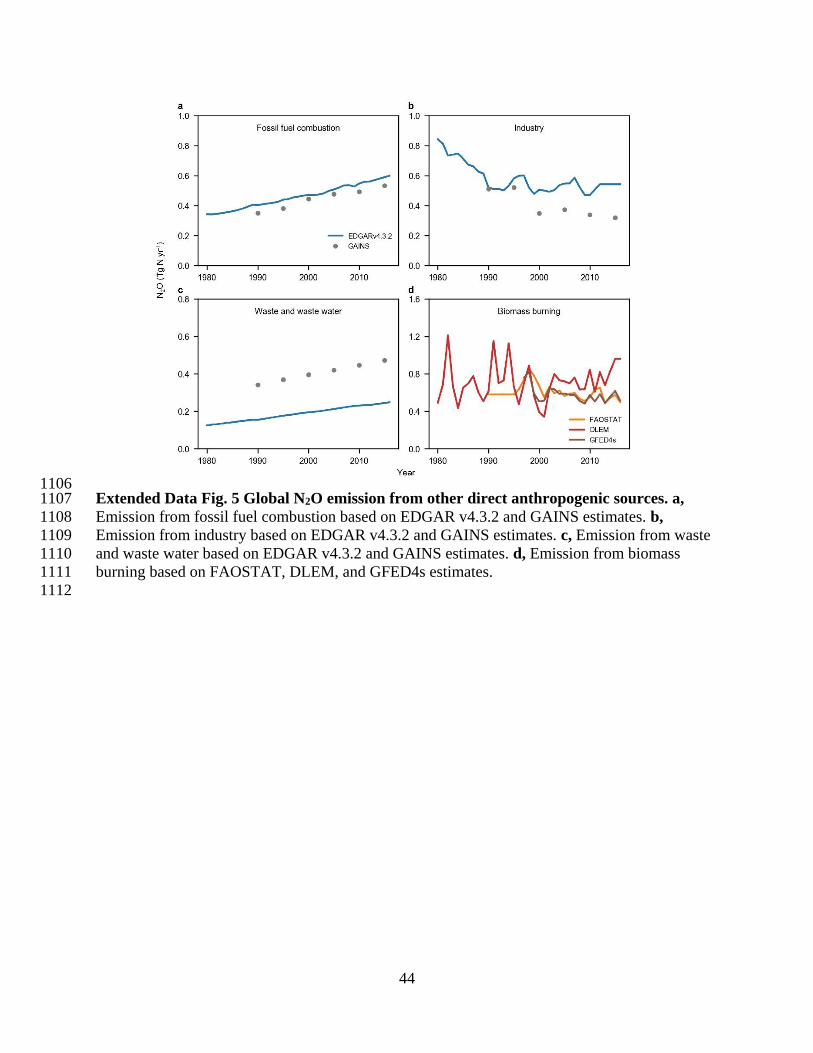
44

1106 Extended Data Fig. 5 Global N2O emission from other direct anthropogenic sources. a, 1107

Emission from fossil fuel combustion based on EDGAR v4.3.2 and GAINS estimates. b, 1108

Emission from industry based on EDGAR v4.3.2 and GAINS estimates. c, Emission from waste 1109

and waste water based on EDGAR v4.3.2 and GAINS estimates. d, Emission from biomass 1110

burning based on FAOSTAT, DLEM, and GFED4s estimates. 1111

1112

45

1113 Extended Data Fig. 6 Global N2O emissions from natural soils, inland and coastal waters 1114

and due to change in climate, atmospheric CO2 and N deposition. a, Changes in global soil 1115

N2O fluxes due to changing CO2 and climate. b, Global natural soil N2O emissions without 1116

consideration of land use change (e.g., deforestation) and without consideration of indirect 1117

anthropogenic effects via global change (i.e., climate, elevated CO2, and atmospheric N 1118

deposition). The estimates are based on NMIP estimates during 1980−2016 including six 1119

process-based land biosphere models. Here, we also subtracted the difference between with and 1120

without consideration of secondary forests emissions that grow back after pasture or cropland 1121

abandonment from natural soil emissions based on NMIP estimates. The solid lines represent the 1122

ensemble and dashed lines show the minimum and maximum values. c, Global anthropogenic 1123

N2O emission from inland waters, estuaries, coastal zones based on models (model-based), 1124

FAOSTAT, GAINS, and EDGAR v4.3.2 estimates. d, Emission due to atmospheric N deposition 1125

(NDEP) on land based on NMIP, FAOSTAT/EDGAR v4.3.2, and GAINS/EDGAR v4.3.2. 1126

FAOSTAT/EDGAR v4.3.2 or GAINS/EDGAR v4.3.2 means the combination of agricultural 1127

source from FAOSTAT or GAINS with non-agricultural source from EDGAR v4.3.2. A process-1128

based model DLEM36 and a mechanistic stochastic model35,51 were used to estimate N2O 1129

emission from inland waters and estuaries, while site-level emission rates of N2O were upscaled 1130

to estimate global N2O fluxes from the global seagrass area68. 1131

1132

1133

46

1134 Extended Data Fig. 7 Global N2O dynamics due to land cover changes. The blue line 1135

represents the mean forest N2O reduction caused by the long-term effect of reduced mature forest 1136

area (i.e., deforestation) and shaded areas show minimum and maximum estimates; the red line 1137

represents the mean N2O emission from post-deforestation pulse effect (i.e., crop/pasture N2O 1138

emissions from legacy N of previous forest soil, not accounting for new fertilizer N added to 1139

these crop/pasture lands) and shaded areas show minimum and maximum estimates; the gray line 1140

represents the mean net deforestation emission of N2O and shaded areas show minimum and 1141

maximum estimates. 1142

1143

1144

47

1145 Extended Data Fig. 8 Global simulated N2O emission anomaly due to climate effect and 1146

global annual land surface temperature anomaly during 1901−2016. Global N2O emission 1147

anomalies are the ensemble of six process-based land biosphere models in NMIP. The 1148

temperature data were obtained from the CRU-NCEP v8 climate dataset 1149

(https://vesg.ipsl.upmc.fr). The above left figure a) shows the correlation between average global 1150

annual land surface temperature and simulated N2O emissions (i.e., the result of SE6 experiment 1151

in NMIP16) considering annual changes in climate but keeping all other factors (i.e., N fertilizer, 1152

manure, NDEP, elevated CO2, and land cover change) at the level of 1860. The above right 1153

figure b) shows the correlation between average global annual land surface temperature and 1154

simulated N2O emissions (i.e., the result of SE1 experiment in NMIP16) considering annual 1155

changes in all factors during 1860−2016. 1156

1157

1158

48

1159 Extended Data Fig. 9 Direct soil emissions and agricultural product trades in Brazil. a, Red 1160

line shows the ensemble direct N2O emissions from livestock manure based on EDGAR v4.3.2, 1161

GAINS, and FAOSTAT, the sum of ‘manure left on pasture’ and ‘manure management’; The 1162

gray columns show the amount of beef export by Brazil. b, Orange line shows the ensemble 1163

direct N2O emissions from croplands due to N fertilization based on NMIP and SRNM; The gray 1164

columns show the amount of soybean and corn exports by Brazil. The data of beef and cereal 1165

product trades were adapted from the ABIEC (beef) and FAOSTAT (soybean and corn). Mmt yr-1166 1 represents millions of metric tons per year. 1167

1168

1169

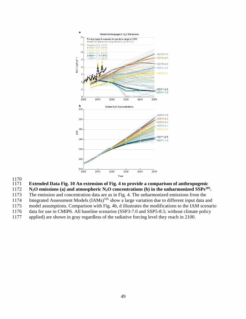
49

1170 Extended Data Fig. 10 An extension of Fig. 4 to provide a comparison of anthropogenic 1171

N2O emissions (a) and atmospheric N2O concentrations (b) in the unharmonized SSPs105. 1172

The emission and concentration data are as in Fig. 4. The unharmonized emissions from the 1173

Integrated Assessment Models (IAMs)105 show a large variation due to different input data and 1174

model assumptions. Comparison with Fig. 4b, d illustrates the modifications to the IAM scenario 1175

data for use in CMIP6. All baseline scenarios (SSP3-7.0 and SSP5-8.5; without climate policy 1176

applied) are shown in gray regardless of the radiative forcing level they reach in 2100. 1177

Supplementary Information

A comprehensive quantification of global nitrous oxide sources and sinks

Hanqin Tian1, Rongting Xu1, Josep G. Canadell2, Rona L. Thompson3, Wilfried Winiwarter4,5, Parvadha Suntharalingam6, Eric A. Davidson7, Philippe Ciais8, Robert B. Jackson9,10,11, Greet Janssens-Maenhout12,13, Michael J. Prather14, Pierre Regnier15, Naiqing Pan1,16, Shufen Pan1, Glen P. Peters17, Hao Shi1, Francesco N. Tubiello18, Sönke Zaehle19, Feng Zhou20, Almut Arneth21, Gianna Battaglia22, Sarah Berthet23, Laurent Bopp24, Alexander F. Bouwman25,26,27, Erik T. Buitenhuis6,28, Jinfeng Chang8,29, Martyn P. Chipperfield30,31, Shree R. S. Dangal32, Edward Dlugokencky33, James W. Elkins33, Bradley D. Eyre34, Bojie Fu16,35, Bradley Hall33, Akihiko Ito36, Fortunat Joos22, Paul B. Krummel37, Angela Landolfi38,39, Goulven G. Laruelle15, Ronny Lauerwald8,15,40, Wei Li8,41, Sebastian Lienert22, Taylor Maavara42, Michael MacLeod43, Dylan B. Millet44, Stefan Olin45, Prabir K. Patra46,47, Ronald G. Prinn48, Peter A. Raymond42, Daniel J. Ruiz14, Guido R. van der Werf49, Nicolas Vuichard8, Junjie Wang27, Ray F. Weiss50, Kelley C. Wells44, Chris Wilson30,31, Jia Yang51 & Yuanzhi Yao1

1International Center for Climate and Global Change Research, School of Forestry and Wildlife Sciences, Auburn University, Auburn, AL, USA 2Global Carbon Project, CSIRO Oceans and Atmosphere, Canberra, Australian Capital Territory, Australia 3Norsk Institutt for Luftforskning, NILU, Kjeller, Norway 4International Institute for Applied Systems Analysis, Laxenburg, Austria 5 Institute of Environmental Engineering, University of Zielona Góra, Zielona Góra, Poland. 6School of Environmental Sciences, University of East Anglia, Norwich, UK 7Appalachian Laboratory, University of Maryland Center for Environmental Science, Frostburg, MD, USA 8Laboratoire des Sciences du Climat et de l'Environnement, LSCE, CEA CNRS, UVSQ UPSACLAY, Gif sur Yvette, France 9Department of Earth System Science, Stanford University, Stanford, CA, USA 10Woods Institute for the Environment, Stanford University, Stanford, CA, USA 11Precourt Institute for Energy, Stanford University, Stanford, CA, USA 12European Commission, Joint Research Centre (JRC), Ispra, Italy 13Ghent University, Faculty of Engineering and Architecture, Ghent, Belgium 14Department of Earth System Science, University of California Irvine, Irvine, CA, USA 15Department Geoscience, Environment & Society, Université Libre de Bruxelles, Brussels, Belgium 16State Key Laboratory of Urban and Regional Ecology, Research Center for Eco-Environmental Sciences, Chinese Academy of Sciences, Beijing, China 17CICERO Center for International Climate Research, Oslo, Norway 18Statistics Division, Food and Agriculture Organization of the United Nations, Via Terme di Caracalla, Rome, Italy 19Max Planck Institute for Biogeochemistry, Jena, Germany

20Sino-France Institute of Earth Systems Science, Laboratory for Earth Surface Processes, College of Urban and Environmental Sciences, Peking University, Beijing, China

21Karlsruhe Institute of Technology, Institute of Meteorology and Climate Research/Atmospheric Environmental Research, Garmisch-Partenkirchen, Germany 22Climate and Environmental Physics, Physics Institute and Oeschger Centre for Climate Change Research, University of Bern, Bern, Switzerland 23Centre National de Recherches Météorologiques (CNRM), Université de Toulouse, Météo‐France, CNRS, Toulouse, France 24LMD-IPSL, Ecole Normale Supérieure / PSL Université, CNRS; Ecole Polytechnique, Sorbonne Université, Paris, France 25PBL Netherlands Environmental Assessment Agency, The Hague, The Netherlands 26Department of Earth Sciences – Geochemistry, Faculty of Geosciences, Utrecht University, Utrecht, The Netherlands 27Key Laboratory of Marine Chemistry Theory and Technology, Ministry of Education, Ocean University of China, Qingdao, China 28Tyndall Centre for Climate Change Research, School of Environmental Sciences, University of East Anglia, Norwich, UK 29College of Environmental and Resource Sciences, Zhejiang University, Hangzhou, China. 30National Centre for Earth Observation, University of Leeds, Leeds, UK 31Institute for Climate and Atmospheric Science, School of Earth and Environment, University of Leeds, Leeds, UK 32Woods Hole Research Center, Falmouth, MA, USA 33NOAA Global Monitoring Laboratory, Boulder, CO, USA 34Centre for Coastal Biogeochemistry, School of Environment Science and Engineering, Southern Cross University, Lismore, New South Wales, Australia 35Faculty of Geographical Science, Beijing Normal University, Beijing, China 36Center for Global Environmental Research, National Institute for Environmental Studies, Tsukuba, Japan 37Climate Science Centre, CSIRO Oceans and Atmosphere, Aspendale, Victoria, Australia 38 GEOMAR Helmholtz Centre for Ocean Research Kiel, Kiel, Germany 39Istituto di Scienze Marine, Consiglio Nazionale delle Ricerche (CNR), Rome, Italy 40Université Paris-Saclay, INRAE, AgroParisTech, UMR ECOSYS, Thiverval-Grignon, France 41Ministry of Education Key Laboratory for Earth System modeling, Department of Earth System Science, Tsinghua University, Beijing, China 42Yale School of Forestry and Environmental Studies, New Haven, CT, USA 43Land Economy, Environment & Society, Scotland’s Rural College (SRUC), Edinburgh, UK 44Department of Soil, Water, and Climate, University of Minnesota, St Paul, MN, USA 45Department of Physical Geography and Ecosystem Science, Lund University, Lund, Sweden 46Research Institute for Global Change, JAMSTEC, Yokohama, Japan 47Center for Environmental Remote Sensing, Chiba University, Chiba, Japan 48Center for Global Change Science, Massachusetts Institute of Technology, Cambridge, MA, USA 49Faculty of Science, Vrije Universiteit, Amsterdam, Netherlands. 50 Scripps Institution of Oceanography, University of California San Diego, La Jolla, USA

51Department of Forestry, Mississippi State University, Mississippi State, MS, USA

Supporting text

1. Data sources .................................................................................................................................1

2. Detailed description on multiple approaches ...............................................................................3

2.1 NMIP – Global N2O Model Inter-comparison Project ...........................................................3

2.2. The FAOSTAT inventory .....................................................................................................5

2.3. The EDGAR v4.3.2 inventory ...............................................................................................7

2.4. The GAINS inventory ...........................................................................................................8

2.5. The SRNM model .................................................................................................................9

a. Flux upscaling model ............................................................................................................9

b. Global cropland N2O observation dataset ..........................................................................10

c. Gridded input datasets ........................................................................................................11

2.6. Global N flow in aquaculture ..............................................................................................11

2.7. Model-based ocean N2O fluxes ...........................................................................................12

2.8. Net N2O emission from land cover change .........................................................................13

a. Deforestation area and crop/pasture expansion ..................................................................13

c. Secondary tropical forest emissions. ..................................................................................14

2.9. Inland water, estuaries, coastal zones ..................................................................................15

a. Riverine N2O emission simulated by DLEM .....................................................................15

b. The DLEM estimate on N2O emission from global reservoirs ..........................................16

c. Mechanistic Stochastic Modeling of N2O emissions from rivers, lakes, reservoirs and

estuaries ..................................................................................................................................16

d. Coastal zone emissions .......................................................................................................18

2.10. Atmospheric inversion models ..........................................................................................18

3. Atmospheric N2O observations and growth rates for three different atmospheric networks

(NOAA, AGAGE, and CISRO) .........................................................................................21

4. Comparison with the IPCC AR5................................................................................................23

5. Per capita N2O emission at global and regional scales in the recent decade .............................24

Supporting tables

Supplementary Table 1 N2O emissions from global agricultural soils based on multiple bottom-up approaches including the additions of mineral N fertilizer, manure and crop residues, and cultivation of organic soils. .........................................................................................32

Supplementary Table 2 N2O emissions from global total area under permanent meadows and pasture, due to manure N deposition (left on pasture) based on EDGAR v4.3.2, FAOSTAT, and GAINS estimates. ....................................................................................32

Supplementary Table 3 N2O emissions due to global manure management based on multiple bottom-up approaches. .......................................................................................................33

Supplementary Table 4 Aquaculture N2O emissions based on multiple sources. .........................33 Supplementary Table 5 Anthropogenic N2O emissions from the global inland waters based on

process-based models.........................................................................................................34 Supplementary Table 6 Anthropogenic N2O emissions from the global inland waters based on

multiple bottom-up approaches. .........................................................................................34 Supplementary Table 7 Natural N2O emissions from the global inland waters based on process-

based models. .....................................................................................................................35 Supplementary Table 8 Nitrous oxide emissions due to atmospheric N deposition on land based

on multiple bottom-up approaches.....................................................................................35 Supplementary Table 9 Global N2O emissions from waste and waste water based on EDGAR

v4.3.2 and GAINS estimates. .............................................................................................36 Supplementary Table 10 Global N2O emissions from fossil fuel and industry based on multiple

bottom-up approaches. .......................................................................................................36 Supplementary Table 11 Global N2O emissions from biomass burning based on multiple bottom-

up approaches.....................................................................................................................37 Supplementary Table 12 Global oceanic N2O emissions based on multiple models. ...................37 Supplementary Table 13 Global N2O emissions based on multiple top-down approaches. ..........38 Supplementary Table 14 Comparison of terminologies used in this study and previous reports. .39 Supplementary Table 15 Comparison of the global N2O budget in this study with the IPCC AR5.

............................................................................................................................................40 Supplementary Table 16 Simulation experiments in the NMIP (Tian et al.1,17) ............................41 Supplementary Table 17 Information of NMIP models using in this study ..................................41 Supplementary Table 18 Summary of models in ocean N2O inter-comparison ............................42 Supplementary Table 19 Overview of the inversion frameworks that are included in the global

N2O budget.........................................................................................................................42

Supporting figures

Supplementary Fig. 1 Spatial distribution of ten study regions across the globe. .........................43

Supplementary Fig. 2 Per capita N2O emission (kg N capita-1 yr-1) during 2007−2016. ..............44

1

1. Data sources

Bottom-up methods include process-based models (NMIP1 including six process‐based terrestrial

biosphere models, DLEM-only2 for pastureland, five ocean models3-8, one mechanistic stochastic

model9,10), four GHG emission databases [EDGAR v4.3.211, FAOSTAT12, GAINS13, GFED4s14

(only for biomass burning), and one statistical model (SRNM) only for cropland soils15. The top-

down approach includes four independent atmospheric inversion frameworks16. The NMIP result

provides nitrous oxide (N2O) emissions from natural and agricultural soils, defined as soils in

agricultural land, during 1860−2016, with consideration of multiple environmental factors, such

as climate, elevated atmospheric carbon dioxide (CO2), land cover and land use change,

atmospheric nitrogen (N) deposition, mineral N fertilizer, and manure N in cropland17. Mineral N

fertilizer and manure N are mainly applied to cropland, while N deposition can reach soils under

all land uses. Natural soil emissions were estimated by NMIP based on the ensemble mean of six

models (Supplementary Table 16): (1) the Dynamic Land Ecosystem Model (DLEM)18,19, (2)

Land Processes and eXchanges model - Bern (LPX-Bern v1.4)20,21, (3) O-CN22, (4) Organising

Carbon and Hydrology In Dynamic Ecosystems (ORCHIDEE)23, (5) Organising Carbon and

Hydrology In Dynamic Ecosystems-Carbon Nitrogen Phosphorus (ORCHIDEE-CNP)23, and (6)

Vegetation Integrated SImulator for Trace gases (VISIT)24,25 (See more model information in

Tian et al.1,17). Agricultural soil emissions were from manure and fertilizer N applications on

cropland during 1860−20161 and intensively managed grassland (pastures) during 1900−20142.

For ‘Indirect emissions from anthropogenic N additions’, we considered emissions from

atmospheric N deposition and ‘Inland and coastal waters’ N leaching/runoff including five sub-

systems: rivers, lakes, estuaries, reservoirs, and coastal zones. Yao et al.26 estimated N2O

emissions from rivers using the process-based model (DLEM) during 1900−2016 and provided

estimates from reservoirs as well, while emissions determined from the stochastic mechanistic

model of Maavara et al.10 and Lauerwald et al.9 for the river-reservoir-estuary continuum, and

lakes, respectively, were in 2000. Coastal zone emissions were obtained from data compilation

reported in Camillini et al.27 and Murray et al.28. The DLEM model also provided an estimate of

N2O emissions from biomass burning across various biomes (crop residue and savannas,

peatland, tropical forest, temperate forest, and boreal forest) during 1860−2015. A nutrient

budget model for shellfish and finfish29-31 was used to calculate the nutrient flows in aquaculture

2

production systems. For computing the N2O emission we consider the amount of N released to

the environment, i.e. the difference between N intake and N in the harvested fish, which includes

all the nutrient excretion. Estimates of oceanic N2O fluxes are derived from an inter-comparison

of five global ocean biogeochemistry models including Bern-3D3, NEMOv3.6-PISCESv2-gas4,

NEMO-PlankTOM105, UVic2.96, and NEMO-PISCES 3.27.

The EDGAR v4.3.2 applies the IPCC guidelines mostly at Tier-1, but integrates higher tier

information based on available country reporting, mostly from Annex I countries. It provided

data from 1970 to 2012. We updated the data to 2016 based on the global and regional trends

between 2000 and 2012 for each individual category. In EDGAR v4.3.2, ‘Indirect emission from

N deposition’ only represents non-agricultural activities. ‘Waste and waste water’ includes

‘Waste incineration’ and ‘Wastewater handling’. We merged ‘Transportation’, ‘Energy’,

‘Industry’, and ‘Residential and other sectors’ to represent the total emission from ‘Fossil fuel

and industry’. Since the EDGAR v4.3.2 database did not provide the emission of ‘Biomass

burning’ from land use outside of agriculture, here we did not include its estimate of ‘Agriculture

waste burning’ into the data synthesis. The FAOSTAT emissions database of the Food and

Agriculture Organization of the United Nations (FAO) covers emissions of N2O from agriculture

and land use by country and globally, from 1961 to 2017 for agriculture, and from 199012 for

relevant land use categories, i.e, cultivation of histosols, biomass burning, etc., applying only

Tier-1 coefficients32. In addition to the IPCC agriculture burning categories ‘Burning crop

residues’ and ‘Burning savannah’, FAOSTAT also estimates N2O emissions from deforestation

fires, forest fires and peatland fires. Emissions from ‘Fossil fuel and industry’ are directly

adapted from the EDGAR v4.3.2 emission inventory. The GAINS model13 provided N2O

emissions data every five-years (i.e., 1990, 1995, 2000, 2005, 2010, 2015). We assumed the

change between each five-year estimate was linear. To avoid abrupt jumps between 1989 and

1990 during data synthesis, we linearly extrapolated data to 1980 through using estimates in

1990 and 1995 in each sub-sector. ‘Direct soil emissions’ are from synthetic N fertilizer, animal

manure, cultivation of histosols, and crop residues. ‘Indirect emissions from anthropogenic N

additions’ are from ‘N deposition on land’ and ‘Inland and coastal waters’ (i.e., lakes, rivers, and

shelf seas). The source of ‘N deposition on land’ is mainly from agricultural activities, but it

deposited on all global ice-free areas (i.e., agricultural land, forest land, other land uses). The

‘Energy’ emission includes conversion, industry, transport, and domestic. The ‘Industry’

3

emission includes nitric acid plants, adipic acid plants, and caprolactam plants. We merged

‘Energy’ and ‘Industry’ to represent ‘Fossil fuel and industry’ emissions. They also considered

N2O use, but we did not include this sector in the synthesis table. We merged ‘Composting’ and

‘Wastewater’ sectors into ‘Waste and waste water’ to make comparison with the EDGAR v4.3.2

database. In addition, the sector ‘Grazing’ was treated as ‘Manure left on pasture’ to make

comparison. The GFED4s emission inventory14 provided N2O emissions from ‘Biomass burning’

including agricultural waste and other biomass burning (i.e., Savanna, grassland, and shrubland

fires, boreal forest fires, temperate forest fires, deforestation and degradation, and peatland fires)

during 1997−2016.

The spatially-referenced non-linear model SRNM was fitted through considering

environmental factors and N management practices to generate gridded annual EF maps at 5′

spatial resolution, and then to calculate global/regional N2O emissions during 1901−2016

together with time-series N input datasets15. This database provides N2O emissions from global

and regional cropland with the application of synthetic N fertilizer and manure N for the period

1980−2016.

For the top-down constraints on the global and regional N2O emissions for the period

1998−2016, we have used estimates from four independent atmospheric inversion frameworks

(INVICAT, PyVAR, MIROC4-ACTM, and GEOSChem), all of which used the Bayesian

inversion method. Here, two versions of PyVAR were run using different ocean priors (one high

and one low) for determining the sensitivity to the ocean prior. These runs are denoted as

PyVAR-1 and PyVAR-2, respectively. For the top-down global estimate, we used the original

spatial resolution in each framework. For the top-down regional estimate, we interpolated the

coarse resolution into 1° × 1° to cover all land areas in the four frameworks (see details in

section 2.10).

2. Detailed description on multiple approaches

2.1 NMIP – Global N2O Model Inter-comparison Project

Ten process-based Terrestrial Biosphere Models (TBMs) participate in NMIP. In general, N2O

emissions from soil are regulated at two levels, which are the rates of nitrification and

denitrification in the soil and soil physical factors regulating the ratio of N2O to other nitrous

4

gases33. For N input to land ecosystems, all ten models considered the atmospheric N deposition

and biological fixation, nine models with crop N2O module included N fertilizer use, but only six

models considered manure as N input. For vegetation processes, all models included dynamic

algorithms in simulating N allocation to different living tissues and vegetation N turnover, and

simulated plant N uptake using the “Demand and Supply-driven” approach. For soil N processes,

all ten models simulated N leaching according to water runoff rate; however, models are

different in representing nitrification and denitrification processes and the impacts of soil

chemical and physical factors. The differences in simulating nitrification and denitrification

processes are one of the major uncertainties in estimating N2O emissions. Algorithms associated

with N2O emissions in each participating model are briefly described in Appendix A of Tian et

al.17.

All participating models are driven by consistent input datasets (i.e., climate, atmospheric

CO2 concentration, land cover change, atmospheric N deposition, mineral N fertilization, and

manure N application) and implemented seven simulation experiments (SE0 – SE6;

Supplementary Table 17) at the spatial resolution of 0.5° globally covering the period of 1861–

2016 (ref. 1). The SE1 includes all driving factors for models with manure addition, and the SE2

is the experiment including all the driving factors for models except manure N. In the SE0

simulation, driving forces were kept constant at the level in 1860 over the entire simulation

period (1861−2016).

By comparing results from different model scenarios, it is possible to attribute the changed

spatiotemporal variations of soil N2O emissions to the variations of six natural and

anthropogenic factors, namely, climate (CLIM, including precipitation, humidity, temperature

and photosynthetic active radiation changes), atmospheric CO2 concentration (CO2), land cover

change (LCC), atmospheric N deposition (NDEP), mineral N fertilizer use (NFER), and manure

N use in cropland (MANN). In order to understand soil N2O emissions dynamics caused by crop

cultivation, we further separated the global and regional N2O emissions into those derived from

cropland soils and those from soils of other land ecosystems. All soils in other land ecosystems

except cropland were treated as “natural soils” while model simulations were implemented in

this study. Except for cropland, the current NMIP simulations do not include management

5

practices (such as grazing and forest logging) for other managed ecosystems such as pasture,

planted forests and urban.

In this study, we aimed to attribute the impact of single factor on cropland N2O emissions,

thus participating models without providing SE2−SE6 and SE0 results in cropland were

excluded. Here, we included estimates from six process-based models (Supplementary Table 16).

Four models (DLEM, ORCHIDEE, ORCHIDEE-CNP, and VISIT) considered the effects of

manure N application in cropland and ran all the seven simulation experiments (SE0−SE6),

while the other two models (LPX-Bern and O-CN) did not include manure effects and ran six

model experiments (all except SE1). We used four model results (i.e., DLEM, ORCHIDEE,

ORCHIDEE-CNP, and VISIT) to calculate the manure N effect (SE1−SE2). Meanwhile, we

used six model results (i.e., DLEM, LPX-Bern, O-CN, ORCHIDEE, ORCHIDEE-CNP, and

VISIT) to calculate the effects of synthetic N fertilizer use (SE2−SE3) and atmospheric N

deposition (SE3−SE4). The effect of N deposition in natural vegetation was calculated from the

six models mentioned above.

2.2. The FAOSTAT inventory

The FAOSTAT emissions data are computed at Tier 1 following IPCC, 2006, Vol. 4. The overall

equation is as follows:

Direct emissions are estimated at country level, using the formula:

Emission = A * EF (1a)

where emission represents kg N yr-1; A represents amount of N in the following items (annual

synthetic N applications/manure applied to soils/manure left on pasture/manure treated in

manure management systems/crop residue/biomass burned amount) in kg N yr-1; EF = Tier 1,

default IPCC emission factors, expressed in kg N/kg N.

Indirect emissions are estimated at country level, using the formula:

Emission = Av&l * EF (1b)

6

where emission represents kg N yr-1; A v&l represents the fraction of manure/synthetic N

fertilizers that volatize as NH3 and NOx and are lost through runoff and leaching in kg N yr-1; EF

= Tier 1, default IPCC emission factors, expressed in kg N/kg N.

Synthetic N fertilizers: N2O from synthetic fertilizers is produced by microbial processes of

nitrification and denitrification taking place on the addition site (direct emissions), and after

volatilization/redeposition and leaching processes (indirect emissions).

Manure management: The term manure includes both urine and dung (i.e., both liquid and

solid material) produced by livestock. N2O is produced directly by nitrification and

denitrification processes in the manure, and indirectly by N volatilization and redeposition

processes.

Manure applied to soils: N2O is produced by microbial processes of nitrification and

denitrification taking place on the application site (direct emissions), and after

volatilization/redeposition and leaching processes (indirect emissions).

Manure left on pastures: N2O is produced by microbial processes of nitrification and

denitrification taking place on the deposition site (direct emissions), and after

volatilization/redeposition and leaching processes (indirect emissions).

Crop Residue: N2O emissions from crop residues consist of direct and indirect emissions from

N in crop residues left on agricultural fields by farmers and from forages during pasture renewal

(following the definitions in the IPCC guidelines34). Specifically, N2O is produced by microbial

processes of nitrification and denitrification taking place on the deposition site (direct

emissions), and leaching processes (indirect emissions).

Cultivation of organic soils: The FAOSTAT domain “Cultivation of organic soils” contains

estimates of direct N2O emissions associated with the drainage of organic soils – histosols –

under cropland and grazed grassland.

Burning-savanna: N2O emissions from the burning of vegetation biomass in the land cover

types: Savanna, Woody Savanna, Open Shrublands, Closed Shrublands, and Grasslands.

Burning-crop residues: N2O produced by the combustion of a percentage of crop residues burnt

on-site. Burning-biomass: N2O emissions from the burning of vegetation biomass in the land

cover types: Humid tropical forest, other forest, and organic soils.

7

2.3. The EDGAR v4.3.2 inventory

The new online version, EDGAR v4.3.2 incorporates a full differentiation of emission processes

with technology-specific emission factors and additional end-of-pipe abatement measures6 and

as such updates and refines the emission estimates. The emissions are modelled based on latest

scientific knowledge, available global statistics, and methods recommended by IPCC (2006)34.

Official data submitted by the Annex I countries to the United Nations Framework Convention

on Climate Change (UNFCCC) and to the Kyoto Protocol are used to some extent, particularly

regarding control measures implemented since 1990 that are not described by international

statistics.

The N2O emission factor for direct soil emissions of N2O from the use of synthetic fertilizers

and from manure used as fertilizers and from crop residues is taken from IPCC (2006)34, that

updated the default IPCC emission factor in the IPCC Good Practice Guidance (2000) with a

20% lower value. N2O emissions from the use of animal waste as fertilizer are estimated taking

into account both the loss of N that occurs from manure management systems before manure is

applied to soils and the additional N introduced by bedding material. N2O emissions from

fertilizer use and CO2 from urea fertilization are estimated based on IFA and FAO statistics.

N2O emissions from manure management are based on distribution of manure management

systems from Annex I countries reporting to the UNFCCC, Zhou et al.35 for China and IPCC

(2006)34 for the rest of the countries.

Different N2O emission factors are applied to tropical and non-tropical regions. N and dry

matter content of agricultural residues are estimated from the cultivation area and yield for 24

crop types (two types of beans, barley, cassava, cereals, three types of peas, lentils, maize, millet,

oats, two types of potatoes, pulses, roots and tubers, rice, rye, soybeans, sugar beet, sugar cane,

sorghum, wheat and yams) from FAOSTAT (2014) and using emission factors of IPCC (2006)34.

Indirect N2O emissions from leaching and runoff of nitrate are estimated from N input to

agricultural soils as described above. Leaching and runoff are assumed to occur in all agricultural

areas except non-irrigated dryland regions, which are identified with maps of FAO Geonetwork

(2011). The fraction of N lost through leaching and runoff is based on the study of Van Drecht et

al.36. The updated emission factor for indirect N2O emissions from N leaching and run-off from

8

the IPCC (2006) guidelines is selected, while noting that it is 70% lower than the mean value of

the 1996 IPCC Guidelines and the IPCC Good Practice Guidance (IPCC, 1997, 2000).

Indirect N2O emissions from atmospheric deposition of N of NOx and NH3 emissions from

non-agricultural sources, mainly fossil fuel combustion, are estimated using N in NOx and NH3

emissions from these sources as activity data, based on EDGAR v4.3.2 database for these gases.

The same emission factor from IPCC (2006)34 is used for indirect N2O from atmospheric

deposition of N from NH3 and NOx emissions, as for agricultural emissions.

2.4. The GAINS inventory

The methodology adopted for the estimation of current and future greenhouse gas emissions and

the available potential for emission controls follows the standard methodology used by the

Greenhouse Gas - Air Pollution Interactions and Synergies (GAINS) model37. For a given year,

emissions of each pollutant p are calculated as the product of the activity levels, the

“uncontrolled” emission factor in the absence of any emission control measures, the efficiency of

emission control measures and the application rate of such measures:

𝐸𝐸𝑖𝑖,𝑝𝑝 = ∑ 𝐸𝐸𝑖𝑖,𝑗𝑗,𝑎𝑎,𝑡𝑡,𝑝𝑝𝑗𝑗,𝑎𝑎,𝑡𝑡 = ∑ 𝐴𝐴𝑖𝑖,𝑗𝑗,𝑎𝑎𝑒𝑒𝑒𝑒𝑖𝑖,𝑗𝑗,𝑎𝑎,𝑝𝑝𝑗𝑗,𝑎𝑎,𝑡𝑡 (1 − 𝑒𝑒𝑒𝑒𝑒𝑒𝑡𝑡,𝑝𝑝 )𝑋𝑋𝑖𝑖,𝑗𝑗,𝑎𝑎,𝑡𝑡 (2)

where subscripts i,j,a,t,p denote region, sector, activity, abatement technology, and pollutant,

respectively; Ei,p represents emissions of the specific pollutant p in region i; Aj represents

activity in a given sector j; ef represents “uncontrolled” emission factor; eff represents reduction

efficiency; X represents actual implementation rate of the considered abatement.

Results (emissions from all anthropogenic sources) are available in 5-year intervals from 1990

to 2050 (in some regions up to 2070) for each GAINS region, typically comprising one country

to express areas of common legislation also with respect of air pollution. Very large countries

have been further split along administrative areas, while in cases of limited data availability also

groups of countries have been combined into GAINS regions.

For N2O, the fate of emissions abatement is often connected with action taken to control other

pollutants. For example, it may occur that after control (e.g., of NOx emissions), N2O emissions

become higher than in the unabated case. To reflect this effect, negative reduction efficiencies

would need to be used for N2O. As it is difficult to communicate such negative numbers, GAINS

9

has resorted to present “controlled” emission factors instead, which describe the emission factor

of a process after installation of abatement technology.

2.5. The SRNM model

a. Flux upscaling model

The SRNM model38 was applied to simulate direct cropland-N2O emissions. In SRNM, N2O

emissions were simulated from N application rates using a quadratic relationship, with spatially-

variable model parameters that depend on climate, soil properties, and management practices.

The original version of SRNM was calibrated using field observations from China only39. In this

study, we used the global N2O observation dataset to train it to create maps of gridded annual

emission factors of N2O and the associated emissions at 5-minute resolution from 1901 to

201415. The gridded EF and associated direct cropland-N2O emissions are simulated based on the

following equation:

2 , ijt ij ijt ij ijt ijtE N N i= + + ∀α β ε (3a)

where

( ) ( )2 2~ , , ~ ,ij k ijk ijk ij k ijk ijkk k

N x N x ′ ∑ ∑α λ σ β φ σ (3b)

( ) ( ) ( )2 2 2~ , , ~ , , ~ 0,ijk ijk ijk ijk ijk ijk ijtN N Nλ µ ω φ µ ω ε τ′ ′ (3c)

and i denotes the sub-function of N2O emission (i=1, 2, …, I) that applies for a sub-domain

division iΩ of six climate or soil factors, j represents the type of crop (j=1-2, 1 for upland crops

and 2 for paddy rice), k is the index of climate or soil factors (k=1-6, i.e., soil pH, clay content,

soil organic carbon, bulk density, the sum of cumulative precipitation and irrigation, mean daily

air temperature). iΩ denotes a set of the range of multiple xk. Eijt denotes direct N2O emission

flux (kg N ha−1 yr−1) estimated for crop type j in year t in the ith sub-domain, Nijt is N application

rate (kg N ha−1 yr−1), and αij and βij are defined as summation of the product of xk and λijk over k.

The random terms λ and φ are assumed to be independent and normally distributed, representing

10

the sensitivity of α and β to xk. ε is the model error. µ and µ′ are the mean effect of xk for α and

β, respectively. σ, σ′, ω, ω′, andτ are standard deviations. Optimal sub-domain division,

associated parameters mean values and standard deviations were determined by using the

Bayesian Recursive Regression Tree version 2 (BRRT v2)39-41, constrained by the extended

global cropland-N2O observation dataset. The detailed methodological approach of the BRRT v2

is described in Zhou et al.41

b. Global cropland N2O observation dataset

We aggregated cropland N2O flux observation data from 180 globally distributed observation

sites from online databases, on-going observation networks, and peer-reviewed publications.

Chamber-based observations were only included in this dataset. These data repositories are as

follows: the NitroEurope, CarbonEurope, GHG-Europe (EU-FP7), GRACEnet, TRAGnet,

NANORP, and 14 meta-analysis datasets42-55. Four types of data were excluded from our

analysis: (i) observations without a zero-N control for background N2O emission, (ii)

observations from sites that used controlled-release fertilizers or nitrification inhibitors, (iii)

observations not covering the entire crop growing season, (iv) observations made in laboratory or

greenhouse. We then calculated cropland-N2O emissions as the difference between observed

N2O emission (E) and background N2O emission (E0). Values of EF were estimated for each

nonzero N application rate (Na) as direct cropland-N2O emission divided by Na: EF = (E −

E0)/Na. This yielded a global dataset of direct cropland-N2O emissions, N-rate-dependent N2O

EFs and fertilization records from each site (i.e., 1,052 estimates for upland crops from 152 sites

and 154 estimates for paddy rice from 28 sites), along with site-level information on climate,

soils, crop type, and relevant experimental parameters. Total numbers of sites and total

measurements in the dataset were more than doubled those for previous datasets of N2O EF. The

extended global N2O observation network covered most of fertilized croplands, representing a

wide range of environmental conditions globally. For each site in our dataset, the variables

included four broad categories: N2O emissions data, climate data (cumulative precipitation and

mean daily air temperature), soil attributes (soil pH, clay content, SOC, BD), and management-

related or experimental parameters (N application rate, crop type). More details on global

cropland N2O observation dataset can be found in Wang et al.15

11

c. Gridded input datasets

The updated SRNM model was driven by many input datasets, including climate, soil properties,

N inputs (e.g., synthetic N fertilizer, livestock manure and crop residues applied to cropland), as

well as the historical distribution of cropland. Cumulative precipitation and mean daily air

temperature over the growing season were acquired from the CRU TS v3.23 climate dataset43

(0.5-degree resolution), where growing season in each grid cell was identified following Sacks et

al.52 The patterns of SOC, clay content, BD, and soil pH were acquired from the HWSD v1.2

(ref.56, 1-km resolution). Both climate and soil properties were re-gridded at a resolution of 5′ ×

5′ using a first-order conservative interpolation widely used in the CMIP5 model

intercomparison57. Annual cropland area at 5′ spatial resolution from 1901 to 2014 was obtained

from the History Database of the Global Environment (HYDE 3.2.1)58. N inputs of synthetic

fertilizers were generated based on sub-national statistics (i.e., county-, municipal, provincial or

state-levels) of N-fertilizer consumption of 15,593 administrative units from 38 national

statistical agencies and national statistics of the other 197 countries from FAOSTAT. N inputs of

livestock manure and crop residues applied to cropland were provided by Zhang et al.59 and

FAOSTAT, respectively. To compute crop-specific N application rates, we allocated N inputs

for upland crops and paddy rice based on the breakdown (or proportion) of total fertilizer use by

crop from Rosas60. Crop-specific N application rates (Nijt) were finally resampled into grid maps

at 5′ spatial resolution following the dynamic cropland distributions of the HYDE 3.2.1. The

assumption of a maximum combined synthetic + manure + crop residues N application rate was

1,000 kg N ha−1, larger than the previous threshold61 that was only applied for the sum of

synthetic fertilizers and manure.

2.6. Global N flow in aquaculture

We apply a nutrient budget model for shellfish and finfish62-64 to calculate the nutrient flows in

aquaculture production systems. These flows comprise feed inputs, retention in the fish, and

nutrient excretion. Individual species within crustaceans, seaweed, fish and molluscs are

aggregated to the International Standard Statistical Classification of Aquatic Animals and Plants

(ISSCAAP) groups65, for which production characteristics are specified. Feed and nutrient

conversion rates are used for each ISSCAAP group to calculate the feed and nutrient intake from

12

production data from FAO65. Feed types include home-made aquafeeds and commercial

compound feeds with different feed conversion ratios that also vary in time due to efficiency

improvement; in addition, the model accounts for algae in ponds, that are often fertilized with

commercial fertilizers or animal manure, consumed by omnivore fish species like carp. A special

case is the filter-feeding bivalves that filter seston from the water column, and excrete

pseudofeces, feces and dissolved nutrients. Based on production data and tissue/shell nutrient

contents the model computes the nutrient retention in the fish. Using apparent digestibility

coefficients, the model calculates outflows in the form of feces (i.e. particulate nutrients) and

dissolved nutrients. Finally, nutrient deposition in pond systems and recycling is calculated. For

computing the N2O emission we consider the amount of N released to the environment, i.e. the

difference between N intake and N in the harvested fish, which includes all the nutrient

excretion. Since in pond cultures part of that N is managed, we made the amount of N recycling

explicit, as well as ammonia emissions from ponds. This is to avoid double counting when

computing N2O emissions from crop production.

2.7. Model-based ocean N2O fluxes

Oceanic N2O is produced by microbial activity during organic matter cycling in the subsurface

ocean; its production mechanisms display significant sensitivity to ambient oxygen level. In the

oxic ocean, N2O is produced as a byproduct during the oxidation of ammonia to nitrate, mediated

by ammonia oxidizing bacteria and archaea. N2O is also produced and consumed in sub-oxic and

anoxic waters through the action of marine denitrifiers during the multi-step reduction of nitrate

to gaseous N. The oceanic N2O distribution therefore displays significant heterogeneity with

background levels of 10-20 nmol/l in the well-oxygenated ocean basins, high concentrations (>

40 nmol/l) in hypoxic waters, and N2O depletion in the core of ocean oxygen minimum zones

(OMZs).

Oceanic N2O emissions are estimated to account for up to a third of the pre-industrial N2O

fluxes to the atmosphere, however, the natural cycle of ocean N2O has been perturbed in recent

decades by inputs of anthropogenically derived nutrient (via atmospheric deposition and riverine

fluxes), and by the impacts of climate change (via impacts on biological productivity and ocean

deoxygenation).

13

Estimates of oceanic N2O fluxes for the Global N2O Budget synthesis are derived from an

inter-comparison of five global ocean biogeochemistry models that include explicit

representation of the oceanic N2O cycle (Supplementary Table 18). Ocean biogeochemistry

models include process representation of ocean circulation, nutrient cycling and trace-gas

generation. In particular, the N2O fluxes to the atmosphere are derived from N2O cycle

parameterizations embedded in the ocean biogeochemistry models and combined with a

parameterization of gas-exchange across the air-sea interface. The models participating in this

inter-comparison are taken from the recent studies of Battaglia and Joos3, Berthet et al.4,

Buitenhuis et al.5, Landolfi et al.6, and Martinez-Rey et al.7.

The models differ in aspects of physical configuration (e.g., spatial resolution),

meteorological forcing applied at the ocean surface, and in their parameterizations of ocean

biogeochemistry; specific details on individual models are provided in the publications listed in

Supplementary Table 18. Towards the N2O budget synthesis, all modelling groups reported

annual mean estimates of ocean-atmosphere N2O fluxes for the period 1980−2016 (or for as

many years as possible in that period). Fluxes were reported at the following spatial scales: (a)

global; (b) Southern latitudes (90°−30°S); (c) Tropics (30°S−30°N); and (d) Northern latitudes

(30°−90°N). In addition, four modelling groups reported annually averaged ocean N2O fluxes at

higher spatial resolution; i.e., gridded to a 1o × 1o resolution.

2.8. Net N2O emission from land cover change

a. Deforestation area and crop/pasture expansion

Two sets of deforestation area were used to represent land cover changes during 1860−2016. The

LUH2 v2h (land use harmonization, http://luh.umd.edu) land use forcing data were used to

derive the deforestation area and its partition between crops and pastures from 1860−2016.

LUH2 categorizes forest lands into forested primary land and potentially forested secondary

land, while croplands are divided into C3 annual crops, C3 perennial crops, C4 annual crops, C4

perennial crops, and C3 N-fixing crops. In the empirical computation, all sub-classes within each

land use type were treated the same. Thus only the annual transition area from forests to

croplands or managed pasture was needed.

14

In the process-based estimates, the model requires input of the plant functional types (PFTs)

of the forests (e.g., tropical broadleaf evergreen forest and tropical broadleaf deciduous forest),

and the species of croplands (e.g., wheat and rice). Thus, a potential vegetation map and the

accompanied composition ratio map of each natural PFT acquired from the Synergetic Land

Cover Product (SYNMAP) were jointly used with LUH2 v2h to generate the historical spatial

distribution of PFTs.

b. Methods

Here we ran the DLEM model with varying climate and CO2 but hold other factors constant to

estimate forest baseline emissions and unfertilized crop/pasture emissions from 1860-2016. The

climate data were acquired from CRU-NCEP v7 (https://vesg.ipsl.upmc.fr), which is a fusion of

the CRU and NCEP/NCAR reanalysis products at a spatial resolution of 0.5° × 0.5° and a daily

time-step. The atmospheric CO2 data were obtained from NOAA GLOBLVIEW-CO2 dataset

(https://www.esrl.noaa.gov), which are derived from atmospheric and ice core measurements. In

the tropical area, both estimates from the DLEM model and the bookkeeping method were

adopted, whereas in extra-tropical area, we only adopted the DLEM outputs.

c. Secondary tropical forest emissions

There are not many published studies on N2O emissions from secondary tropical forests that

grow back after crop or pasture abandonment. A recent meta-analysis by Sullivan et al.66 lumps

together all forms of N "gas loss" including NO and N2O, so it does not address N2O

specifically. It also reviews the data for secondary forests across the tropics and shows that eight

N cycling parameters, including N gas loss and some other parameters that overlap with those

measured by Davidson et al.67 and Keller and Reiners68, recover only gradually during secondary

tropical forest succession. Their meta-analysis of the N gas loss parameter showed a significant

positive slope, indicating gradually increasing gas loss rates with age after initiation of secondary

forest regrowth66. Keller and Reiners68 showed a gradual recovery of soil nitrate and soil

emissions of N2O and nitric oxide (NO) during 20 years of secondary forest succession. As

shown, N2O emissions did not return to the level of the primary forest after about 20 years of

secondary forest succession. Davidson et al.67 found that it takes 40−70 years of secondary forest

succession for N2O emissions to approach levels of the primary forest. This is also consistent

with other trends of related N cycling parameters, such as the nitrate:ammonium ratio, soil

15

nitrate, litter mass:N, litterfall N:P, and foliar 15N. In this study, through using the sites of field

observation from Davidson et al.67 and Keller and Reiners68, we estimated N2O emission from

secondary tropical forests based on the algorithm: y=0.0084x + 0.2401 (R2 = 0.44). ). x (unit:

year) indicates secondary forest age and y (unitless; 0−1) indicates the ratio of secondary forest

N2O emission over that of a reference mature forest. The difference between primary forests and

secondary forests were subtracted from natural soil emissions simulated by six land-surface

models in NMIP.

2.9. Inland water, estuaries, coastal zones

a. Riverine N2O emission simulated by DLEM

Here we developed a riverine N2O module within a scale adaptive water transport model and

coupled with the DLEM model15. The land surface module of DLEM-simulated N species

(NO3⁻, NH4⁺, DON and PON) leaching from soils when N inputs were into the water transport

model. The river routine module within the DLEM is a fully distributed water transport model,

which explicitly calculated the flow routine cell-to-cell based on hydraulics methods. The water

quality module built into the water transport module can simulate the carbon lateral

transportation, biogeochemical reactions (e.g., decomposition of organic matter, nitrification,

denitrification), CO2 degassing and physical deposition of particle organic matter and has been

successfully applied in the Gulf of Mexico and the U.S. east coast69-75. Specifically, by

introducing sub-grid routine processes technology into the model, the scale adaptive water

transport module can effectively address the physical and biogeochemical processes of the small

streams within a grid cell, which has been overly simplified in earth system models. We

validated global N fluxes based on GEMS-GLORI world river discharge database. The newly

developed riverine N2O module receives dissolved N2O from land and groundwater, atmosphere

wet deposition, and calculate the dynamics of dissolved N2O concentration and fluxes in both

small streams and large rivers. Here, we validated the annual mean riverine N2O concentration,

ground water N2O concentration, and riverine N2O emissions globally based on literature survey.

DLEM simulated results all agree well with the observations.

16

b. The DLEM estimate on N2O emission from global reservoirs

We assumed the reservoirs were linked to rivers, and thus these aquatic systems shared the

similar N2O emission rates in the large-scale studies. We therefore estimate the reservoir surface-

area form the Global Reservoirs and Dams (GRanD) database. In riverine N2O fluxes

estimations, we have two N2O fluxes rates: one is the emission from the large river channel, and

the other one is the emission from small rivers within the grid cell. We obtained the upstream

area of each dam from the GRanD database and overlaid with the area raster of the 0.5° cell. If

the upstream area of a dam is less than the area of its belonging 0.5° grid cell, we considered the

dam was located at the small streams within the grid cell and the fluxes of that dam equal to the

small river N2O fluxes of that grid. On the contrary, if the upstream area was larger than the area

of the grid cell, the dam is located at the large river channel, thus the fluxes of that dam equal to

the riverine N2O fluxes of the main channel in that grid cell. Align with uncertainty analysis in

the riverine N2O estimations, we overlaid the surface area of dams with riverine N2O emission

rate estimates from the nine-uncertainty experiments to get the reservoir N2O emissions. We

calculated the average as the final reported value.

c. Mechanistic Stochastic Modeling of N2O emissions from rivers, lakes, reservoirs and estuaries

In our calculations, we used a process-oriented model recently developed to estimate N2O

emissions from inland waters, including rivers, reservoirs and estuaries10. To estimate N2O

emissions from lakes9, we applied the same approach to a global lake dataset76. Based on a

spatially explicit representation of water bodies and point and non-point sources of N and

phosphorus (P), this model quantifies the global scale spatial patterns in inland water N2O

emissions in a consistent manner at 0.5° resolution. The methodology is based on the application

of a stochastic Monte Carlo-based model to estimate average annual rates of primary production,

ammonification, nitrification, denitrification, N fixation and burial of N in sediments as well as

N2O production and emission generated by nitrification and denitrification. Because of the

scarcity of observations, the Monte Carlo approach is a necessary step to generate predictive

equations for the N budget and N2O emission of each inland water body based on inputs of total

N (TN) and total P (TP) from the watershed and water residence times in a given river segment,

lake, reservoir or estuary9,10. In situ N cycling processes for each specific water body worldwide

cannot be predicted due to the lack of parameter constraints or data at this fine granularity.

17

Instead, the model is fed with hypothetical but realistic combinations of physical and

biogeochemical parameters through the use of probability density functions (PDFs)

approximating the global statistical distribution of those parameters as derived from literature

values and databases. A Monte Carlo analysis of the model is then performed, in which

parameters are stochastically selected from the pre-assigned PDFs. After several thousand

iterations spanning the entire parameter space of physical and biogeochemical characteristics, a

database of hypothetical worldwide N dynamics, including N2O production and emissions, is

generated for river, lake, reservoir, and estuarine systems. Then, global relationships relating N

processes and N2O emissions to TN and TP loads and water residence time are fitted from the

database and applied for the global upscaling.

To calculate the cascading loads of TN and TP delivered to each water body along the river–

reservoir–estuary continuum, we spatially routed all reservoirs from the GRanD database77, with

river networks from Hydrosheds 15s78 and, at latitudes above 50°N, Hydro1K (USGS, 2000),

which were in turn connected to estuaries as represented in the “Worldwide Typology of

Nearshore Coastal Systems” of Dürr et al.79. In addition, the global data base HydroLAKES76

was used to topologically connect 1.4 million lakes with a minimum surface area of 0.1 km2

within the river network. Note that besides natural lakes, HydroLAKES includes updated

information on 6,796 reservoirs from the GRanD data base, which was used in the study of

Maavara et al.10. In order to estimate the TN and TP loads to each water body, we then relied on

a spatially explicit representation of TN and TP mobilization from the watershed into the river

network (see Maavara et al. for details80,81).

For the estimation of N2O emission, we applied two distinct model configurations,

respectively named DS1 and DS2 in Maavara et al.10. DS1 estimates N2O emissions from

denitrification and nitrification based on an EF of 0.9%, which is in the mean of published

values82, and the assumption that N2O production equals N2O emissions10. For DS2, the

reduction of N2O to N2 during denitrification if N2O is not evading sufficiently rapidly from the

water body is taken into account. The fluxes in the model represent lumped sediment-water

column rates and were resolved at the annual timescale. The use of water residence time as

independent variable in both the mechanistic model and the upscaling process introduces an

important kinetic refinement to existing global N2O emission estimates. Rather than applying an

average EF (directly scaling N2O emissions to N inputs) to all water bodies, the use of water

18

residence time explicitly adjusts for the extent of N2O production and emission that is kinetically

possible within the timeframe available in a given water body. Simulated N2O emission rates

were evaluated against measurement-based upscaling methods applied to reservoirs83 and rivers84

as well as against observation-driven regional estimates of lake N2O emissions based on

literature data9.

d. Coastal zone emissions

The average of net N2O fluxes from three seagrass species27 (seagrasses, mangroves, saltmarsh

and intertidal) was scaled to the global seagrass area28. The mangrove data from Murray et al.28

was updated with water-air and sediment-air N2O fluxes from Maher et al.85 and Murray et al.86.

The average sediment-air N2O flux and the average water-air N2O flux were each applied for 12

hours a day (see Rosentreter et al.87), and scaled to the global mangrove area28. Murray et al.28

saltmarsh data was updated with sediment-air N2O fluxes from Yang et al.88, Chmura et al.89, Welti

et al.90 and Roughan et al.91 and scaled to the global saltmarsh area28. Murray et al.28 intertidal data

was updated with sediment-air N2O fluxes from Moseman-Valtierra et al. 92 and Sun et al.93 and

scaled to the global intertidal area94.

2.10. Atmospheric inversion models

Emissions were estimated using four independent atmospheric inversion frameworks (see

Supplementary Table 19). The frameworks all used the Bayesian inversion method, which finds

the optimal emissions, that is, those, which when coupled to a model of atmospheric transport,

provide the best agreement to observed N2O mixing ratios while being guided by the prior

estimates and their uncertainty. In other words, the optimal emissions are those that minimize the

cost function:

(5a)

where x and xb are, respectively, vectors of the optimal and prior emissions, B is the prior error

covariance matrix, y is a vector of observed N2O mixing ratios, R is the observation error

covariance matrix, and H(x) is the model of atmospheric transport (for details on the inversion

19

method see95). The optimal emissions, x, were found by solving the first order derivative of

equation (5a):

(5b)

where (H′(x))T is the adjoint model of transport. In frameworks INVICAT, PyVAR and

GEOSChem, equation (5b) was solved using the variational approach96-98, which uses a descent

algorithm and computations involving the forward and adjoint models. In framework MIROC4-

ACTM, equation (5b) was solved directly by computing a transport operator, H from

integrations of the forward model, such that Hx is equivalent to H(x), and taking the transpose of

H99.

Each of the inversion frameworks used a different model of atmospheric transport with

different horizontal and vertical resolutions (see Supplementary Table 19). The transport models

TOMCAT and LMDz5, used in INVICAT and PyVAR respectively, were driven by ECMWF

ERA-Interim wind fields, MIROC4-ACTM, was driven by JRA-55 wind fields, and GEOSChem

was driven by MERRA-2 wind fields. While INVICAT, PyVAR, and GEOSChem optimized the

emissions at the spatial resolution of the transport model, MIROC4-ACTM optimized the error

in the emissions aggregated into 84 land and ocean regions. All frameworks optimized the

emissions with monthly temporal resolution. The transport models included an online calculation

of the loss of N2O in the stratosphere due to photolysis and oxidation by O(1D) resulting in mean

atmospheric lifetimes of between 118 and 129 years, broadly consistent with recent independent

estimates of the lifetime of 116±9 years (ref. 100).

All inversions used N2O measurements of discrete air samples from the National Oceanic and

Atmospheric Administration Carbon Cycle Cooperative Global Air Sampling Network (NOAA).

In addition, discrete measurements from the Commonwealth Scientific and Industrial Research

Organisation network (CSIRO) as well as in-situ measurements from the Advanced Global

Atmospheric Gases Experiment network (AGAGE), the NOAA CATS network, and from

individual sites operated by University of Edinburgh (UE), National Institute for Environmental

Studies (NIES) and the Finnish Meteorological Institute (FMI) were included in INVICAT,

PyVAR and GEOSchem. Measurements from networks other than NOAA were corrected to the

NOAA calibration scale, NOAA-2006A, using the results of the WMO Round Robin inter-

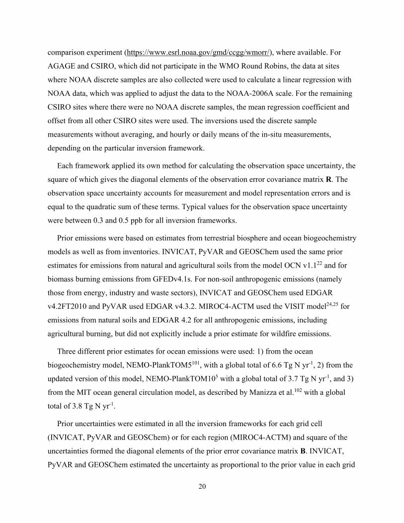
20

comparison experiment (https://www.esrl.noaa.gov/gmd/ccgg/wmorr/), where available. For

AGAGE and CSIRO, which did not participate in the WMO Round Robins, the data at sites

where NOAA discrete samples are also collected were used to calculate a linear regression with

NOAA data, which was applied to adjust the data to the NOAA-2006A scale. For the remaining

CSIRO sites where there were no NOAA discrete samples, the mean regression coefficient and

offset from all other CSIRO sites were used. The inversions used the discrete sample

measurements without averaging, and hourly or daily means of the in-situ measurements,

depending on the particular inversion framework.

Each framework applied its own method for calculating the observation space uncertainty, the

square of which gives the diagonal elements of the observation error covariance matrix R. The

observation space uncertainty accounts for measurement and model representation errors and is

equal to the quadratic sum of these terms. Typical values for the observation space uncertainty

were between 0.3 and 0.5 ppb for all inversion frameworks.

Prior emissions were based on estimates from terrestrial biosphere and ocean biogeochemistry

models as well as from inventories. INVICAT, PyVAR and GEOSChem used the same prior

estimates for emissions from natural and agricultural soils from the model OCN v1.122 and for

biomass burning emissions from GFEDv4.1s. For non-soil anthropogenic emissions (namely

those from energy, industry and waste sectors), INVICAT and GEOSChem used EDGAR

v4.2FT2010 and PyVAR used EDGAR v4.3.2. MIROC4-ACTM used the VISIT model24,25 for

emissions from natural soils and EDGAR 4.2 for all anthropogenic emissions, including

agricultural burning, but did not explicitly include a prior estimate for wildfire emissions.

Three different prior estimates for ocean emissions were used: 1) from the ocean

biogeochemistry model, NEMO-PlankTOM5101, with a global total of 6.6 Tg N yr-1, 2) from the

updated version of this model, NEMO-PlankTOM105 with a global total of 3.7 Tg N yr-1, and 3)

from the MIT ocean general circulation model, as described by Manizza et al.102 with a global

total of 3.8 Tg N yr-1.

Prior uncertainties were estimated in all the inversion frameworks for each grid cell

(INVICAT, PyVAR and GEOSChem) or for each region (MIROC4-ACTM) and square of the

uncertainties formed the diagonal elements of the prior error covariance matrix B. INVICAT,

PyVAR and GEOSChem estimated the uncertainty as proportional to the prior value in each grid

21

cell, but MIROC4-ACTM set the uncertainty uniformly for the land regions at 1 Tg N yr-1 and

for the ocean regions at 0.5 Tg N yr-1.

3. Atmospheric N2O observations and growth rates for three different

atmospheric networks (NOAA, AGAGE, and CISRO)

The monthly atmospheric N2O abundances and their growth rates are derived from three

different atmospheric observational networks (AGAGE, CISRO and NOAA) (Extended Data

Fig. 1).

For atmospheric N2O observations from the NOAA network103, we used global mean mixing

ratios from the GMD combined dataset during 1980−2017 based on measurements from five

different measurement programs [HATS old flask instrument, HATS current flask instrument

(OTTO), CCGG group Cooperative Global Air Sampling Network

(https://www.esrl.noaa.gov/gmd/ccgg/flask.php), HATS in situ (RITS program), and HATS in

situ (CATS program)]. CCGG provides uncertainties with each measurement (see site files:

ftp://aftp.cmdl.noaa.gov/data/greenhouse_gases/n2o/flask/surface/). Global means are derived

from flask and in situ measurements obtained by gas chromatography with electron capture

detection, from 4−12 sites (fewer sites in the earlier years), weighted by representative area.

Monthly mean observations from different NOAA measurement programs are statistically

combined to create a long-term NOAA/ESRL GMD dataset. Uncertainties (1 sigma) associated

with monthly estimates of global mean N2O, are ~1 ppb from 1977−1987, 0.6 ppb from

1988−1994, 0.3−0.4 ppb from 1995−2000, and 0.1 ppb from 2001−2017. NOAA data are

generally more consistent after 1995, with standard deviations on the monthly mean mixing

ratios at individual sites of ~0.5 ppb from 1995−1998, and 0.1−0.4 ppb after 1998. A detailed

description of these measurement programs and the method to combine them are available via

https://www.esrl.noaa.gov/gmd/hats/combined/N2O.html.

The Advanced Global Atmospheric Gases Experiment (AGAGE) global network (and its

predecessors ALE and GAGE)104 has made continuous high frequency gas chromatographic

measurements of N2O at five globally distributed sites since 1978. AGAGE includes two types

of instruments [i.e., a gas chromatograph with multiple detectors (GC-MD) and a gas

22

chromatograph with preconcentration and mass spectrometric analysis (Medusa GC-MS)]. The

measurement precision for N2O improved from about 0.35% in ALE to 0.13% in GAGE105 and

0.05% in AGAGE104. We used the global mean of N2O measurements from the GC-MD during

1980−2017. Further information on AGAGE stations, instruments, calibration, uncertainties and

access to data is available at the AGAGE website: http://agage.mit.edu.

The CSIRO flask network106 consists of nine sampling sites distributed globally and has been

in operation since 1992. Flask samples are collected approximately every two weeks and shipped

back to CSIRO GASLAB for analysis. Samples were analyzed by gas chromatography with

electron capture detection (GC-ECD). One Shimadzu gas chromatograph, labelled “Shimadzu-1”

(S1) was used over the entire length of the record and the measurement precision for N2O from

this instrument is about 0.1%. N2O data from the CSIRO global flask network are reported on the

NOAA-2006A N2O scale and are archived at the World Data Centre for Greenhouse Gases

(WDCGG: https://gaw.kishou.go.jp/). Nine sites from the CSIRO network were used to calculate

the annual global N2O mole fractions. Smooth curve fits to the N2O data from each of these sites

were calculated using the technique outlined in Thoning et al.107, using a short-term cut-off of 80

days. The smooth curve fit data were then placed on an evenly spaced latitude (5 degree) versus

time (weekly) grid using the Kriging interpolation technique. Finally, the gridded data were used

to calculate the global annual average mole fractions weighted by latitude.

We plotted the atmospheric globally averaged N2O abundances and the associated growth

rates for the three global atmospheric networks NOAA, AGAGE, and CSIRO during 1980−2017

(see Extended Data Fig. 1). We see remarkably consistent global mean N2O estimated from the

three different networks, increasing from 301.0±0.1 ppb in 1980 to 329.9±0.4 ppb in 2017.

Growth rates of N2O are also remarkably consistent among the three measurement networks.

After a period in the late 1990s in which the growth rate averaged about 0.8 ppb yr-1, the global

growth rate fell to ~0.6 ppb yr-1 and then gradually increased to nearly 1 ppb yr-1 by 2013−2017.

Interannual variability in the N2O growth rate was higher prior to 1995 (not shown) than after

1995, which may be an artifact of less precise measurements due to changes in instrumental

precision and measurement frequency over the study period. Additional discussion on

uncertainties associated with measurement errors and emission errors in inversions can be found

in Chen and Prinn108 and Thompson et al16.

23

4. Comparison with the IPCC AR5

Our methodology significantly differs from past approaches summarized in the IPCC AR5.

Most of the estimates used in the AR5 (e.g., natural sources) directly inherited or adopted with

minor revisions data from studies conducted mainly in the 1990s. Some estimates used in the

IPCC AR5 (e.g., atmospheric deposition on land) were from a review by Syakila and Kroeze109,

which depended on empirical methods and simple assumptions.

Compared to the findings reported in the IPCC AR5, our budget includes several new

sources (e.g., aquaculture, deforestation/post-deforestation, the effects of environmental factors,

natural sources of inland and coastal waters) and one additional (tropospheric) sink for N2O

(Table 6). We report natural sources of N2O emissions from inland and coastal waters with a

value of 0.3 Tg N yr-1. The total source of N2O in our study is 0.9 Tg N yr-1 smaller than that in

the IPCC AR5, while our estimate of anthropogenic N2O emissions is 0.4 Tg N yr-1 larger in the

recent decade (Supplementary Table 15). Our larger estimate of anthropogenic emissions is

associated with environmental effects (0.2, with a range of -0.6 to 1.1 Tg N yr-1, based on NMIP

simulations), and a 0.4 Tg N yr-1 larger estimate of atmospheric N deposition emissions (based

on modeling results and inventories, Table 1). In contrast, our estimate of direct emissions from

agriculture [(3.8 (2.5−5.8) Tg N yr-1, plus aquaculture, a minor contribution] is 0.3 Tg N yr-1

smaller than reported in the IPCC AR5.

Natural sources in our study are 1.3 Tg N yr-1 smaller than those reported by the IPCC AR5

for 2007−2016 and the range is significantly reduced. The mean NMIP estimate of global natural

soil emission [5.6 (4.9−6.6) Tg N yr-1] is 1.0 Tg N yr-1 smaller compared to those in the IPCC

AR5 estimate [6.6 (3.3−9.0) Tg N yr-1]. The reduction in uncertainty in NMIP estimates may

result from calibration of terrestrial biosphere models in NMIP against in situ observations

across the globe1, while the AR5 estimate, essentially inherited from the AR4 synthesis, was

based on results from a single simple model by Bouwman et al.110.

24

In this study, global oceanic N2O emission is derived from an ensemble of global ocean

biogeochemistry models. Our estimate [3.4 (2.5−4.3) Tg N yr-1] is 0.4 Tg N yr-1 smaller and the

uncertainty range is significantly smaller than reported in the IPCC AR5 (1.8–9.4 Tg N yr-1). The

larger AR5 range was determined using an analysis of Atlantic Ocean surface measurements

(Rhee et al.111; the Atlantic is not a region of significant N2O emission) as the lower bound, and

the upper bound was the maximal value of N2O production from a global empirically based

analysis112. The parameterizations governing marine productivity and N2O yield in our five

ocean models have been constrained by a variety of datasets characterizing marine

biogeochemical process rates, and the model simulations of ocean N2O have been evaluated

against global biogeochemical databases (e.g., see Battaglia and Joos3 and Buitenhuis et al.5 for

more detail). The smaller range of ocean N2O emission reported in this study includes advances

in modeling such factors as quantification of global marine export production, improved

constraints on N2O yield parameters (particularly in the well-oxygenated ocean), and more

comprehensive evaluation of modeled biogeochemical distributions.

The estimated N2O production through atmospheric chemistry is 0.2 Tg N yr-1 smaller than

reported in the IPCC AR5. The observed stratospheric sink of N2O in this study is 0.9 Tg N yr-1

smaller than in the IPCC AR5, wherein stratospheric N2O destruction was tuned to be consistent

with the difference between the total source and the observed atmospheric N2O growth rate. In

our study, stratospheric sinks were obtained from atmospheric chemistry transport models and

the recent post-AR5 study by Prather et al.16,100,113 who calculated N2O stratospheric loss (&

lifetime) based on satellite observations combined with simple photolysis models using observed

atmospheric temperature, O2, and O3. Our uncertainties in the atmospheric loss of N2O (±1.1 Tg

N yr-1) are slightly larger than those of the AR5 (±0.9 Tg N yr-1). In our study, annual change in

atmospheric abundance is calculated from the combined NOAA and AGAGE record of surface

N2O and uncertainty (±0.5 Tg N yr-1) is taken from the IPCC AR5 (ref. 114).

5. Per capita N2O emission at global and regional scales in the recent decade

Per capita N2O emission is calculated using global and regional emissions divided by the

numbers of global and regional population115 (see Supplementary Fig. 2). Global per capita

emissions from top-down and bottom-up approaches were on average ~2 kg N capita-1 yr-1 in the

25

recent decade. Bottom-up estimates show that per capita natural fluxes including natural soils

and inland and coastal waters were the largest source, followed by agriculture and other direct

anthropogenic sources. South America and Oceania have ~2 times and ~6 times higher per capita

emissions than the global average, respectively. Africa and Russia also have higher per capita

N2O emissions than the global value contributed primarily by natural fluxes and to a minor

extent by other direct anthropogenic sources (Africa: Biomass burning; Russia: Fossil fuel and

industry and Biomass burning). In addition, North America and Europe show higher than global

per capita emissions from agriculture and other direct anthropogenic sources (primary from

Fossil fuel and industry). Middle East, East Asia, South Asia, and Southeast Asia show lower

than global per capita emissions from all sources.

26

References: 1 Tian, H. Q. et al. Global soil nitrous oxide emissions since the preindustrial era estimated by an

ensemble of terrestrial biosphere models: Magnitude, attribution, and uncertainty. Global Change Biology 25, 640-659 (2019).

2 Dangal, S. R. et al. Global nitrous oxide emissions from pasturelands and rangelands: Magnitude, spatio‐temporal patterns and attribution. Global Biogeochemical Cycles 33, 200-222 (2019).

3 Battaglia, G. & Joos, F. Marine N2O Emissions From Nitrification and Denitrification Constrained by Modern Observations and Projected in Multimillennial Global Warming Simulations. Global Biogeochemical Cycles 32, 92-121 (2018).

4 Berthet, S. et al. Evaluation of an Online Grid-Coarsening Algorithm in a Global Eddy-Admitting Ocean Biogeochemical Model. Journal of Advances in Modeling Earth Systems 11, 1759-1783 (2019).

5 Buitenhuis, E. T., Suntharalingam, P. & Le Quéré, C. Constraints on global oceanic emissions of N2O from observations and models. Biogeosciences 15, 2161-2175 (2018).

6 Landolfi, A., Somes, C. J., Koeve, W., Zamora, L. M. & Oschlies, A. Oceanic nitrogen cycling and N2O flux perturbations in the Anthropocene. Global Biogeochemical Cycles 31, 1236-1255 (2017).

7 Martinez-Rey, J., Bopp, L., Gehlen, M., Tagliabue, A. & Gruber, N. Projections of oceanic N2O emissions in the 21st century using the IPSL Earth system model. Biogeosciences 12, 4133-4148 (2015).

8 Suntharalingam, P. et al. Estimates of Oceanic Nitrous-oxide Emissions from Global Biogeochemistry Models. American Geophysical Union, Fall Meeting 2018 (2018).

9 Lauerwald, R. et al. Natural lakes are a minor global source of N2O to the atmosphere. Global Biogeochemical Cycles 33, 1564-1581 (2019).

10 Maavara, T. et al. Nitrous oxide emissions from inland waters: Are IPCC estimates too high? Global Change Biology 25, 473-488 (2019).

11 Janssens-Maenhout, G. et al. EDGAR v4.3.2 Global Atlas of the three major greenhouse gas emissions for the period 1970–2012. Earth System Science Data 11, 959-1002 (2019).

12 Tubiello, F. et al. Estimating greenhouse gas emissions in agriculture: a manual to address data requirements for developing countries. FAO, Rome (2015).

13 Winiwarter, W., Höglund-Isaksson, L., Klimont, Z., Schöpp, W. & Amann, M. Technical opportunities to reduce global anthropogenic emissions of nitrous oxide. Environmental research letters 13, 014011 (2018).

14 Van Der Werf, G. R. et al. Global fire emissions estimates during 1997-2016. Earth System Science Data 9, 697-720 (2017).

15 Wang, Q. et al. Data-driven estimates of global nitrous oxide emissions from croplands. National Science Review 00, 1-12 (2019).

16 Thompson, R. L. et al. Acceleration of global N2O emissions seen from two decades of atmospheric inversion. Natural Climate Change 9, 993-998 (2019).

17 Tian, H. Q. et al. The Global N2O Model Intercomparison Project. Bulletin of the American Meteorological Society 99, 1231-1252 (2018).

18 Tian, H. et al. Global methane and nitrous oxide emissions from terrestrial ecosystems due to multiple environmental changes. Ecosystem Health and Sustainability 1, 1-20 (2015).

19 Xu, R. et al. Preindustrial nitrous oxide emissions from the land biosphere estimated by using a global biogeochemistry model. Climate of the Past 13, 977 (2017).

20 Stocker, B. D. et al. Multiple greenhouse-gas feedbacks from the land biosphere under future climate change scenarios. Nature Climate Change 3, 666, doi:10.1038/nclimate1864 (2013).

21 XU-RI & PRENTICE, I. C. Terrestrial nitrogen cycle simulation with a dynamic global vegetation model. Global Change Biology 14, 1745-1764 (2008).

27

22 Zaehle, S., Ciais, P., Friend, A. D. & Prieur, V. Carbon benefits of anthropogenic reactive nitrogen offset by nitrous oxide emissions. Nature Geoscience 4, 601-605 (2011).

23 Goll, D. S. et al. A representation of the phosphorus cycle for ORCHIDEE (revision 4520). Geosci. Model Dev. 10, 3745-3770 (2017).

24 Inatomi, M., Ito, A., Ishijima, K. & Murayama, S. Greenhouse Gas Budget of a Cool-Temperate Deciduous Broad-Leaved Forest in Japan Estimated Using a Process-Based Model. Ecosystems 13, 472-483 (2010).

25 Ito, A., Nishina, K., Ishijima, K., Hashimoto, S. & Inatomi, M. Emissions of nitrous oxide (N2O) from soil surfaces and their historical changes in East Asia: a model-based assessment. Progress in Earth and Planetary Science 5, 55, doi:10.1186/s40645-018-0215-4 (2018).

26 Yao, Y. et al. Increased global nitrous oxide emissions from streams and rivers in the Anthropocene. Natural Climate Change 10, 138-142 (2020).

27 Camillini, N., Rossentreter, J., Erler, D., Glud, R. N. & Eyre, B. Blue carbon burial in seagrass meadows is partially offset by CH4 and N2O fluxes. Science Advance (Submitted).

28 Murray, R. H., Erler, D. V. & Eyre, B. D. Nitrous oxide fluxes in estuarine environments: response to global change. Global Change Biology 21, 3219-3245 (2015).

29 Beusen, A. H., Bouwman, A. F., Van Beek, L. P., Mogollón, J. M. & Middelburg, J. J. Global riverine N and P transport to ocean increased during the 20th century despite increased retention along the aquatic continuum. Biogeosciences 13, 2441-2451 (2016).

30 Bouwman, A. F. et al. Hindcasts and future projections of global inland and coastal nitrogen and phosphorus loads due to finfish aquaculture. Reviews in Fisheries Science 21, 112-156 (2013).

31 Bouwman, A. F. et al. Global hindcasts and future projections of coastal nitrogen and phosphorus loads due to shellfish and seaweed aquaculture. Reviews in Fisheries Science 19, 331-357 (2011).

32 Tubiello, F. N. et al. The FAOSTAT database of greenhouse gas emissions from agriculture. 8, 015009 (2013).

33 Davidson, E. A., Erickson, H. E., Verchot, L. V., Keller, M. & Veldkamp, E. Testing a Conceptual Model of Soil Emissions of Nitrous and Nitric Oxides: Using two functions based on soil nitrogen availability and soil water content, the hole-in-the-pipe model characterizes a large fraction of the observed variation of nitric oxide and nitrous oxide emissions from soils. BioScience 50, 667-680 (2000).

34 IPCC. 2006 IPCC Guidelines for National Greenhouse Gas Inventories., (Japan on behalf of the IPCC, Hayama, Japan, 2006).

35 Zhou, J., Jiang, M. & Chen, G. Estimation of methane and nitrous oxide emission from livestock and poultry in China during 1949–2003. Energy Policy 35, 3759-3767 (2007).

36 Van Drecht, G., Bouwman, A. F., Knoop, J. M., Beusen, A. H. W. & Meinardi, C. R. Global modeling of the fate of nitrogen from point and nonpoint sources in soils, groundwater, and surface water. Global Biogeochemical Cycles 17, 1115, doi:10.1029/2003gb002060 (2003).

37 Amann, M. et al. Cost-effective control of air quality and greenhouse gases in Europe: Modeling and policy applications. Environmental Modelling & Software 26, 1489-1501 (2011).

38 Zhang, X. et al. Managing nitrogen for sustainable development. Nature 528, 51, doi:doi:10.1038/nature15743 (2015).

39 Gao, S. et al. Quantifying nitrogen leaching response to fertilizer additions in China's cropland. Environmental pollution 211, 241-251 (2016).

40 Hou, X. et al. Detection and attribution of nitrogen runoff trend in China's croplands. Environmental pollution 234, 270-278 (2018).

41 Zhou, F. et al. New model for capturing the variations of fertilizer‐induced emission factors of N2O. Global Biogeochemical Cycles 29, 885-897 (2015).

42 Decock, C. Mitigating nitrous oxide emissions from corn cropping systems in the midwestern US: potential and data gaps. Environmental science & technology 48, 4247-4256 (2014).

28

43 Harris, I., Jones, P. D., Osborn, T. J. & Lister, D. H. Updated high‐resolution grids of monthly climatic observations–the CRU TS3. 10 Dataset. International journal of climatology 34, 623-642 (2014).

44 Helgason, B. et al. Toward improved coefficients for predicting direct N2O emissions from soil in Canadian agroecosystems. Nutrient Cycling in Agroecosystems 72, 87-99 (2005).

45 Hénault, C. et al. Predicting in situ soil N2O emission using NOE algorithm and soil database. Global Change Biology 11, 115-127 (2005).

46 Hickman, J. E., Scholes, R. J., Rosenstock, T. S., Garcia-Pando, C. P. & Nyamangara, J. Assessing non-CO2 climate-forcing emissions and mitigation in sub-Saharan Africa. Current Opinion in Environmental Sustainability 9, 65-72 (2014).

47 Kim, D.-G., Giltrap, D. & Hernandez-Ramirez, G. Background nitrous oxide emissions in agricultural and natural lands: a meta-analysis. Plant and soil 373, 17-30 (2013).

48 Kim, D.-G., Hernandez-Ramirez, G. & Giltrap, D. Linear and nonlinear dependency of direct nitrous oxide emissions on fertilizer nitrogen input: A meta-analysis. Agriculture, Ecosystems & Environment 168, 53-65 (2013).

49 Lehuger, S. et al. Predicting and mitigating the net greenhouse gas emissions of crop rotations in Western Europe. Agricultural and forest meteorology 151, 1654-1671 (2011).

50 Leppelt, T. et al. Nitrous oxide emission budgets and land-use-driven hotspots for organic soils in Europe. Biogeosciences (2014).

51 Rochette, P. & Janzen, H. H. Towards a revised coefficient for estimating N2O emissions from legumes. Nutrient Cycling in Agroecosystems 73, 171-179 (2005).

52 Sacks, W. J., Deryng, D., Foley, J. A. & Ramankutty, N. Crop planting dates: an analysis of global patterns. Global Ecol Biogeogr 19, 607-620 (2010).

53 Shcherbak, I., Millar, N. & Robertson, G. P. Global metaanalysis of the nonlinear response of soil nitrous oxide (N2O) emissions to fertilizer nitrogen. Proceedings of the National Academy of Sciences 111, 9199-9204 (2014).

54 Stehfest, E. & Bouwman, L. N2O and NO emission from agricultural fields and soils under natural vegetation: summarizing available measurement data and modeling of global annual emissions. Nutrient Cycling in Agroecosystems 74, 207-228 (2006).

55 Walter, K. et al. Direct nitrous oxide emissions from oilseed rape cropping–a meta‐analysis. GCB Bioenergy 7, 1260-1271 (2015).

56 Berdanier, A. B. & Conant, R. T. Regionally differentiated estimates of cropland N2O emissions reduce uncertainty in global calculations. Global change biology 18, 928-935 (2012).

57 Yang, H. et al. Regional patterns of future runoff changes from Earth system models constrained by observation. Geophysical Research Letters 44, 5540-5549 (2017).

58 Goldewijk, K. K., Beusen, A., Doelman, J. & Stehfest, E. Anthropogenic land use estimates for the Holocene–HYDE 3.2. Earth System Science Data 9, 927-953 (2017).

59 Zhang, B. et al. Global manure nitrogen production and application in cropland during 1860–2014: a 5 arcmin gridded global dataset for Earth system modeling. Earth System Science Data 9, 667-678 (2017).

60 Rosas, F. Fertilizer use by crop at the country level (1990–2010). CARD Working Papers 555 (2012).

61 Carlson, K. M. et al. Greenhouse gas emissions intensity of global croplands. Nature Climate Change 7, 63 (2017).

62 Bouwman, L. et al. Mariculture: significant and expanding cause of coastal nutrient enrichment. Environmental Research Letters 8, 044026, doi:044010.041088/041748-049326/044028/044024/044026 (2013).

63 Bouwman, A. F. et al. Hindcasts and future projections of global inland and coastal nitrogen and phosphorus loads due to finfish aquaculture. Reviews in Fisheries Science 21, 112-156 (2013).

64 Bouwman, A. F. et al. Global hindcasts and future projections of coastal nitrogen and phosphorus loads due to shellfish and seaweed aquaculture. Reviews in Fisheries Science 19, 331-357 (2011).

29

65 FAO. FishStatJ - Software for Fishery and Aquaculture Statistical Time Series. http://www.fao.org/fishery/statistics/software/fishstatj/en. (Fisheries and Aquaculture Information and Statistics Service, Food and Agriculture Organization of the United Nations, retrieved 22 May 2019, Rome, 2019).

66 Sullivan, B. W. et al. Biogeochemical recuperation of lowland tropical forest during succession. Ecology 100, e02641, doi:10.1002/ecy.2641 (2019).

67 Davidson, E. A. et al. Recuperation of nitrogen cycling in Amazonian forests following agricultural abandonment. Nature 447, 995 (2007).

68 Keller, M. & Reiners, W. A. Soil-atmosphere exchange of nitrous oxide, nitric oxide, and methane under secondary succession of pasture to forest in the Atlantic lowlands of Costa Rica. Global Biogeochemical Cycles 8, 399-409 (1994).

69 Liu, M. et al. Long‐term trends in evapotranspiration and runoff over the drainage basins of the Gulf of Mexico during 1901–2008. Water Resources Research 49, 1988-2012 (2013).

70 Ren, W. et al. Century‐long increasing trend and variability of dissolved organic carbon export from the Mississippi River basin driven by natural and anthropogenic forcing. Global Biogeochemical Cycles 30, 1288-1299 (2016).

71 Ren, W. et al. Large increase in dissolved inorganic carbon flux from the Mississippi River to Gulf of Mexico due to climatic and anthropogenic changes over the 21st century. Journal of Geophysical Research: Biogeosciences 120, 724-736 (2015).

72 Tao, B. et al. Increasing Mississippi river discharge throughout the 21st century influenced by changes in climate, land use, and atmospheric CO2. Geophysical Research Letters 41, 4978-4986 (2014).

73 Tian, H. et al. Climate extremes dominating seasonal and interannual variations in carbon export from the Mississippi River Basin. Global Biogeochemical Cycles 29, 1333-1347 (2015).

74 Tian, H. et al. Anthropogenic and climatic influences on carbon fluxes from eastern North America to the Atlantic Ocean: A process‐based modeling study. Journal of Geophysical Research: Biogeosciences 120, 757-772 (2015).

75 Yang, Q. et al. Increased nitrogen export from eastern North America to the Atlantic Ocean due to climatic and anthropogenic changes during 1901–2008. Journal of Geophysical Research: Biogeosciences 120, 1046-1068 (2015).

76 Messager, M. L., Lehner, B., Grill, G., Nedeva, I. & Schmitt, O. Estimating the volume and age of water stored in global lakes using a geo-statistical approach. Nature Communications 7, 13603 (2016).

77 Lehner, B. et al. High-resolution mapping of the world's reservoirs and dams for sustainable river-flow management. Frontiers in Ecology and the Environment 9, 494-502 (2011).

78 Lehner, B., Verdin, K. & Jarvis, A. New global hydrography derived from spaceborne elevation data. Eos, Transactions, American Geophysical Union 89, 93-94 (2008).

79 Dürr, H. H. et al. Worldwide Typology of Nearshore Coastal Systems: Defining the Estuarine Filter of River Inputs to the Oceans. Estuaries and Coasts 34, 441-458 (2011).

80 Bouwman, A., Beusen, A. H. & Billen, G. J. G. B. C. Human alteration of the global nitrogen and phosphorus soil balances for the period 1970–2050. Global Biogeochemical Cycles 23, GB0A04, doi:10.1029/2009GB003576 (2009).

81 Van Drecht, G., Bouwman, A., Harrison, J. & Knoop, J. Global nitrogen and phosphate in urban wastewater for the period 1970 to 2050. Global Biogeochemical Cycles 23, GB0A03 (2009).

82 Beaulieu, J. J. et al. Nitrous oxide emission from denitrification in stream and river networks. Proceedings of the National Academy of Sciences 108, 214-219 (2011).

83 Deemer, B. R. et al. Greenhouse gas emissions from reservoir water surfaces: a new global synthesis. 66, 949-964 (2016).

84 Hu, M., Chen, D. & Dahlgren, R. A. Modeling nitrous oxide (N2O) emission from rivers: A global assessment. Global Change Biology 22, 3566-3582 (2016).

30

85 Maher, D. T., Sippo, J. Z., Tait, D. R., Holloway, C. & Santos, I. R. Pristine mangrove creek waters are a sink of nitrous oxide. Scientific reports 6, 25701 (2016).

86 Murray, R., Erler, D., Rosentreter, J., Maher, D. & Eyre, B. A seasonal source and sink of nitrous oxide in mangroves: Insights from concentration, isotope, and isotopomer measurements. Geochimica et Cosmochimica Acta 238, 169-192 (2018).

87 Rosentreter, J. A., Maher, D. T., Erler, D. V., Murray, R. H. & Eyre, B. D. Methane emissions partially offset “blue carbon” burial in mangroves. Science advances 4, eaao4985 (2018).

88 Yang, W. H. & Silver, W. L. Gross nitrous oxide production drives net nitrous oxide fluxes across a salt marsh landscape. Global Change Biology 22, 2228-2237 (2016).

89 Chmura, G. L., Kellman, L., Van Ardenne, L. & Guntenspergen, G. R. Greenhouse gas fluxes from salt marshes exposed to chronic nutrient enrichment. PloS one 11, e0149937 (2016).

90 Welti, N., Hayes, M. & Lockington, D. Seasonal nitrous oxide and methane emissions across a subtropical estuarine salinity gradient. Biogeochemistry 132, 55-69 (2017).

91 Roughan, B. L., Kellman, L., Smith, E. & Chmura, G. L. Nitrous oxide emissions could reduce the blue carbon value of marshes on eutrophic estuaries. Environmental Research Letters 13, 044034 (2018).

92 Moseman-Valtierra, S. et al. Substantial nitrous oxide emissions from intertidal sediments and groundwater in anthropogenically-impacted West Falmouth Harbor, Massachusetts. Chemosphere 119, 1281-1288 (2015).

93 Sun, W., Sun, Z., Mou, X., Sun, W. & Hu, X. Nitrous oxide emissions from intertidal zone of the Yellow River estuary in autumn and winter during 2011–2012. Estuaries and coasts 40, 145-159 (2017).

94 Murray, N. J. et al. The global distribution and trajectory of tidal flats. Nature 565, 222 (2019). 95 Tarantola, A. Inverse problem theory and methods for model parameter estimation. Vol. 89

(Society for Industrial and Applied Mathematics 2005). 96 Thompson, R. L. et al. Nitrous oxide emissions 1999 to 2009 from a global atmospheric

inversion. Atmospheric Chemistry and Physics 14, 1801-1817 (2014). 97 Wells, K. C. et al. Simulation of atmospheric N2O with GEOS-Chem and its adjoint: evaluation

of observational constraints. Geoscience Model Development 8, 3179-3198 (2015). 98 Wilson, C., Chipperfield, M., Gloor, M. & Chevallier, F. Development of a variational flux

inversion system (INVICAT v1. 0) using the TOMCAT chemical transport model. Geoscientific Model Development 7, 2485-2500 (2014).

99 Patra, P. K. et al. Improved Chemical Tracer Simulation by MIROC4. 0-based Atmospheric Chemistry-Transport Model (MIROC4-ACTM). Sola 14, 91-96 (2018).

100 Prather, M. J. et al. Measuring and modeling the lifetime of nitrous oxide including its variability. Journal of Geophysical Research: Atmospheres 120, 5693-5705 (2015).

101 Suntharalingam, P. et al. Quantifying the impact of anthropogenic nitrogen deposition on oceanic nitrous oxide. Geophysical Research Letters 39, L07605, doi:10.1029/2011GL050778 (2012).

102 Manizza, M., Keeling, R. F. & Nevison, C. D. On the processes controlling the seasonal cycles of the air–sea fluxes of O2 and N2O: A modelling study. Tellus B: Chemical and Physical Meteorology 64, 18429, doi:10.3402/tellusb.v64i0.18429 (2012).

103 Hall, B., Dutton, G. & Elkins, J. The NOAA nitrous oxide standard scale for atmospheric observations. Journal of Geophysical Research: Atmospheres 112, D09305, doi:10.1029/2006JD007954 (2007).

104 Prinn, R. G. et al. History of chemically and radiatively important atmospheric gases from the Advanced Global Atmospheric Gases Experiment (AGAGE). Earth System Science Data 10, 985-1018 (2018).

105 Prinn, R. et al. Atmospheric emissions and trends of nitrous oxide deduced from 10 years of ALE–GAGE data. Journal of Geophysical Research: Atmospheres 95, 18369-18385 (1990).

106 Francey, R. J. et al. The CSIRO (Australia) measurement of greenhouse gases in the global atmosphere. 97-111 (World Meteorological Organization, Tokyo, Japan, 2003).

31

107 Thoning, K. W., Tans, P. P. & Komhyr, W. D. Atmospheric carbon dioxide at Mauna Loa Observatory: 2. Analysis of the NOAA GMCC data, 1974–1985. Journal of Geophysical Research: Atmospheres 94, 8549-8565 (1989).

108 Chen, Y. H. & Prinn, R. G. Estimation of atmospheric methane emissions between 1996 and 2001 using a three‐dimensional global chemical transport model. Journal of Geophysical Research: Atmospheres 111, 307, doi:10.1029/2005JD006058 (2006).

109 Syakila, A. & Kroeze, C. The global nitrous oxide budget revisited. Greenhouse Gas Measurement and Management 1, 17-26 (2011).

110 Bouwman, A., Fung, I., Matthews, E. & John, J. Global analysis of the potential for N2O production in natural soils. Global Biogeochemical Cycles 7, 557-597 (1993).

111 Rhee, T. S., Kettle, A. J. & Andreae, M. O. Methane and nitrous oxide emissions from the ocean: A reassessment using basin-wide observations in the Atlantic. Journal of Geophysical Research: Atmospheres 114, doi:10.1029/2008jd011662 (2009).

112 Bianchi, D., Dunne, J. P., Sarmiento, J. L. & Galbraith, E. D. Data-based estimates of suboxia, denitrification, and N2O production in the ocean and their sensitivities to dissolved O2. Global Biogeochemical Cycles 26, doi:10.1029/2011gb004209 (2012).

113 Prather, M. J. & Hsu, J. Coupling of Nitrous Oxide and Methane by Global Atmospheric Chemistry. Science 330, 952-954 (2010).

114 Ciais, P. et al. in Climate Change 2013: The Physical Science Basis. Contribution of Working Group I to the Fifth Assessment Report of the Intergovernmental Panel on Climate Change 465-570 (Cambridge University Press, 2014).

115 FAOSTAT. Food and Agriculture Organization of the United Nations Statistics-Population, 2020).

116 Hu, Z., Lee, J. W., Chandran, K., Kim, S. & Khanal, S. K. Nitrous oxide (N2O) emission from aquaculture: a review. Environmental science technology 46, 6470-6480 (2012).

117 MacLeod, M., Hasan, M. R., Robb, D. H. F. & Mamun-Ur-Rashid, M. Quantifying and mitigating greenhouse gas emissions from global aquaculture. FAO, Rome, (2019).

32

Supplementary Table 1 N2O emissions from global agricultural soils based on multiple bottom-up approaches including the additions of mineral N fertilizer, manure and crop residues, and cultivation of organic soils. Unit: Tg N yr-1

Data sources 1980s 1990s 2000s 2007-2016

Process-based models

NMIP/DLEM Mean 1.7 2.1 2.4 2.8 NMIP/DLEM Min 0.9 1.1 1.3 1.4 NMIP/DLEM Max 2.6 3.1 3.4 3.8

Statistical model plus DLEM SRNM/DLEM 1.3 1.6 1.9 2.1

Inventories EDGAR v4.3.2 1.3 1.5 1.7 1.9 GAINS 1.5 1.6 1.7 1.9 FAOSTAT 1.2 1.5 1.7 1.9

Mean 1.5 1.8 2.0 2.3 Min 0.9 1.1 1.3 1.4 Max 2.6 3.1 3.4 3.8

Supplementary Table 2 N2O emissions from global total area under permanent meadows and pasture, due to manure N deposition (left on pasture) based on EDGAR v4.3.2, FAOSTAT, and GAINS estimates. Unit: Tg N yr-1

Data sources 1980s 1990s 2000s 2007-2016

EDGAR v4.3.2 1.0 1.1 1.2 1.3 GAINS 0.7 0.7 0.8 0.9 FAOSTAT 1.0 1.1 1.2 1.3 Mean 0.9 1.0 1.1 1.2 Min 0.7 0.7 0.8 0.9 Max 1.0 1.1 1.2 1.3

33

Supplementary Table 3 N2O emissions due to global manure management based on multiple bottom-up approaches. Unit: Tg N yr-1

Data sources 1980s 1990s 2000s 2007-2016 EDGAR v4.3.2 0.2 0.2 0.2 0.2 GAINS 0.4 0.4 0.5 0.5 FAOSTAT 0.2 0.2 0.2 0.2 Mean 0.3 0.3 0.3 0.3 Min 0.2 0.2 0.2 0.2 Max 0.4 0.4 0.5 0.5

Supplementary Table 4 Aquaculture N2O emissions based on multiple sources. Unit: Tg N yr-1

Data sources Emission factor (%) 1980s 1990s 2000s 2007-

2016* Hu et al.116 1.8 N/A N/A N/A 0.1 MacLeod et al.117 1.8 N/A N/A N/A 0.1 Bouwman et al. 1.8 0.01 0.03 0.1 0.1 Bouwman et al._Min 0.5 0.00 0.01 0.02 0.02 Bouwman et al._Max 5.0 0.03 0.1 0.2 0.2

* Estimates in Hu et al.116 and Macleod et al.117 were in 2009 and 2013, respectively. N/A represents data are not available.

34

Supplementary Table 5 Anthropogenic N2O emissions from the global inland waters based on process-based models. Unit: Tg N yr-1

Data sources/sectors 1980s 1990s 2000s 2007-2016 River_DLEM 0.2 0.2 0.2 0.2 River_Maavara 0.03 0.03 0.03 0.03 River_Mean 0.1 0.1 0.1 0.1 Resevoirs_DLEM 0.05 0.05 0.05 0.05 Resevoirs_Maavara 0.03 0.03 0.03 0.03 Resevoirs_Mean 0.04 0.04 0.04 0.04 Estuaries_Maavara 0.1 0.1 0.1 0.1 Lake_Lauerwald 0.02 0.02 0.02 0.02 Blue carbon_Murray 0.1 0.1 0.1 0.1 Total_Mean 0.3 0.3 0.3 0.3 Total_Min 0.2 0.2 0.2 0.2 Total_Max 0.4 0.4 0.4 0.4

Supplementary Table 6 Anthropogenic N2O emissions from the global inland waters based on multiple bottom-up approaches. Unit: Tg N yr-1

Data sources 1980s 1990s 2000s 2007-2016 FAOSTAT 0.4 0.4 0.5 0.6 GAINS 0.4 0.4 0.5 0.6 EDGAR v4.3.2 0.5 0.5 0.6 0.7 Model-based 0.3 0.3 0.3 0.3 Mean 0.4 0.4 0.4 0.5 Min 0.2 0.2 0.2 0.2 Max 0.5 0.5 0.6 0.7

35

Supplementary Table 7 Natural N2O emissions from the global inland waters based on process-based models. Unit: Tg N yr-1

Data sources/sectors 1980s 1990s 2000s 2007-2016 River_DLEM 0.1 0.1 0.1 0.1 River_Maavara 0.02 0.02 0.02 0.02 River_Mean 0.04 0.04 0.04 0.04 Resevoirs_DLEM 0.04 0.04 0.04 0.04 Resevoirs_Maavara 0.03 0.03 0.03 0.03 Resevoirs_Mean 0.03 0.03 0.03 0.03 Estuaries_Maavara 0.05 0.05 0.05 0.05 Lake_Lauerwald 0.02 0.02 0.02 0.02 Blue carbon_Murray 0.2 0.2 0.2 0.2 Total_Mean 0.3 0.3 0.3 0.3 Total_Min 0.3 0.3 0.3 0.3 Total_Max 0.4 0.4 0.4 0.4

Supplementary Table 8 Nitrous oxide emissions due to atmospheric N deposition on land based on multiple bottom-up approaches. Unit: Tg N yr-1

Data sources 1980s 1990s 2000s 2007-2016 EDGAR v4.3.2 0.3 0.3 0.3 0.4 FAOSTAT 0.3 0.3 0.3 0.4 GAINS 0.3 0.3 0.3 0.4 FAOSTAT/EDGAR v4.3.2 0.6 0.6 0.7 0.8 GAINS/EDGAR v4.3.2 0.6 0.6 0.7 0.7 NMIP_Mean 0.6 0.7 0.8 0.8 NMIP_Min 0.3 0.4 0.4 0.4 NMIP_Max 1.2 1.4 1.3 1.4 Mean 0.6 0.7 0.7 0.8 Min 0.3 0.4 0.4 0.4 Max 1.2 1.4 1.3 1.4

36

Supplementary Table 9 Global N2O emissions from waste and waste water based on EDGAR v4.3.2 and GAINS estimates. Unit: Tg N yr-1

Data sources 1980s 1990s 2000s 2007-2016 EDGAR v4.3.2 0.1 0.2 0.2 0.2 GAINS 0.3 0.4 0.4 0.5 Mean 0.2 0.3 0.3 0.3 Min 0.1 0.2 0.2 0.2 Max 0.3 0.4 0.4 0.5

Supplementary Table 10 Global N2O emissions from fossil fuel and industry based on multiple bottom-up approaches. Unit: Tg N yr-1

Data sources Sectors 1980s 1990s 2000s 2007-2016

EDGAR v4.3.2

Energy 0.1 0.1 0.1 0.2 Transportation 0.2 0.2 0.2 0.2 Others_residential 0.1 0.2 0.2 0.2 Industry 0.7 0.5 0.5 0.5

GAINS Energy 0.3 0.4 0.5 0.5 Industry 0.5 0.5 0.4 0.3 Mean 0.9 0.9 0.9 1.0 Min 0.8 0.9 0.8 0.8 Max 1.1 1.0 1.0 1.1

37

Supplementary Table 11 Global N2O emissions from biomass burning based on multiple bottom-up approaches. Unit: Tg N yr-1

Fire categories Data sources 1980s 1990s 2000s 2007-2016

Crop residues and savannas

GFED4s 0.4 0.4 0.4 FAOSTAT 0.4 0.4 0.3 DLEM 0.3 0.3 0.3 0.4 Mean 0.3 0.4 0.4 0.4

Tropical forests and Deforestation*

GFED4s 0.1 0.1 0.1 FAOSTAT 0.1 0.1 0.1 DLEM 0.2 0.2 0.2 0.2 Mean 0.2 0.1 0.1 0.1

Peatland

GFED4s

0.04 0.01 0.01 FAOSTAT

0.1 0.1 0.1

DLEM 0.04 0.05 0.02 0.02 Mean 0.04 0.06 0.04 0.04

Boreal and temperate forests

GFED4s

0.1 0.1 0.1 FAOSTAT

0.1 0.1 0.1

DLEM 0.1 0.1 0.1 0.1 Mean 0.1 0.1 0.1 0.1

Total_Mean 0.7 0.7 0.6 0.6 Total_Min 0.7 0.5 0.4 0.5 Total_Max 0.7 0.9 0.8 0.8

* DLEM estimates represent burning of tropical forests that are caused by natural and deforestation fires.

Supplementary Table 12 Global oceanic N2O emissions based on multiple models. Unit: Tg N yr-1

Model 1980s 1990s 2000s 2007-2016

Bern-3D 4.4 4.4 4.3 4.3

NEMOv3.6-PISCESv2-gas 3.3 3.2 3.3 3.4

NEMO-PlankTOM10 3.0 2.8 2.7 2.5

UVic2.9 3.3 3.2 3.2 3.1

NEMO-PISCES 3.2 4.0 3.9 3.9 3.8

Mean 3.6 3.5 3.5 3.4

Min 3.0 2.8 2.7 2.5

Max 4.4 4.4 4.3 4.3

38

Supplementary Table 13 Global N2O emissions based on multiple top-down approaches. Unit: Tg N yr-1

Name Category 2000s 2007-2016

INVICAT

Land

Ocean

Total

9.7

7.2

16.9

10.6

7.1

17.7

PyVAR-1

Land

Ocean

Total

9.4

6.4

15.8

10.6

6.4

17.0

PyVAR-2

Land

Ocean

Total

11.8

4.0

15.8

12.7

4.3

17.0

MIROC4-ACTM

Land

Ocean

Total

12.5

3.1

15.7

13.8

3.4

17.1

GEOSChem

Land

Ocean

Total

10.6

4.5

11.3

4.6

15.1 15.9

Mean

Land

Ocean

Total

10.8

5.1

15.9

11.8

5.1

16.9

Min

Land

Ocean

Total

9.4

3.1

15.1

10.6

3.4

15.9

Max

Land

Ocean

Total

12.5

7.2

16.9

13.8

7.1

17.7

39

Supplementary Table 14 Comparison of terminologies used in this study and previous reports.

GCP Terminology (in this study) IPCC AR5 (IPCC, 2013) National GHG inventories (used by UNFCCC according to IPCC, 2006 and IPCC, 2019)

UNFCCC / IPCC 2006 Source sector

Anthropogenic sources

Direct emissions of N additions in the agricultural sector (Agriculture)

Direct soil emissions (mineral N and manure fertilization, cultivation of organic soils, and crop residue returns) Agriculture

Direct N2O emissions from managed soils (except due to grazing animals)

3Da without 3Da3

Manure left on pasture Urine and dung deposited by grazing animals 3Da3 Manure management Manure management 3B Aquaculture --- --- ---

Other direct anthropogenic sources

Fossil fuel and industry Fossil fuel combustion and industrial processes Energy and industrial processes 1, 2

Waste and waste water Human excreta Waste 5 Biomass burning (from crop residue, grassland, shrubland and savannas; peat fires, tropical forests, boreal forests, and temperate forests)

Biomass and biofuel burning

Prescribed burning of savannas, field burning of agricultural residues 3E, 3F

Indirect emissions from anthropogenic N additions

Inland and coastal waters (rivers, lakes, reservoirs, estuaries, and coastal zones)

Rivers, estuaries, coastal zones Indirect emissions due to leaching and runoff 3Db2

Atmospheric N deposition on land Atmospheric deposition on land Indirect emissions due to atmospheric deposition

(of agricultural as well as other anthropogenic compounds emitted)

part of 3Db1

Atmospheric N deposition on ocean Atmospheric deposition on ocean part of 3Db1

Perturbed fluxes from climate/CO2/land cover change

CO2 effect --- --- --- Climate effect --- --- --- Post-deforestation pulse effect --- --- --- Long-term effect of reduced mature forest area --- --- ---

Natural sources and sinks

Natural soils baseline Soils under natural vegetation --- ---

Ocean baseline Oceans --- --- Natural (rivers, lakes, reservoirs, estuaries, and coastal upwelling) --- --- ---

Lightning and atmospheric production Lightning --- --- Atmospheric chemistry --- ---

Soil/wetland surface sink Surface sink --- ---

40

Supplementary Table 15 Comparison of the global N2O budget in this study with the IPCC AR5.

Note: ∗ Calculated from satellite observations combined with simple photolysis models in our study.

This study (2007–2016)

IPCC AR5 (2006/2011)

Bottom-up budget

Anthropogenic Sources Fossil fuel combustion and industry 1.0 (0.8–1.1) 0.7 (0.2–1.8) Agriculture (incl. Aquaculture) 3.8 (2.5–5.8) 4.1 (1.7–4.8) Biomass and biofuel burning 0.6 (0.5–0.8) 0.7 (0.2–1.0) Wastewater 0.3 (0.2–0.5) 0.2 (0.1–0.3) Rivers, estuaries, and coastal zones 0.5 (0.2–0.7) 0.6 (0.1–2.9) Atmospheric N deposition on ocean 0.1 (0.1–0.2) 0.2 (0.1–0.4) Atmospheric N deposition on land 0.8 (0.4–1.4) 0.4 (0.3–0.9) Other indirect effects from CO2, climate and land-use change 0.2 (-0.6–1.1)

Total Anthropogenic 7.3 (4.2–11.4) 6.9 (2.7–12.1)

Natural Sources and Sinks Rivers, estuaries, and coastal zones 0.3 (0.3–0.4) Oceans 3.4 (2.5–4.3) 3.8 (1.8–9.4) Soils under natural vegetation 5.6 (4.9–6.5) 6.6 (3.3–9.0) Atmospheric chemistry 0.4 (0.2–1.2) 0.6 (0.3–1.2) Surface sink -0.01 (0− -0.3) -0.01 (0− -1) Total natural 9.7 (8.0–12.0) 11.0 (5.4–18.6)

Total bottom-up source 17.0 (12.2–23.5) 17.9 (8.1–30.7) Observed growth rate 4.3 (3.8–4.8) 3.6 (3.5–3.8) Tropospheric sink 0.1 (0.1−0.2)

Stratospheric sink∗ 13.4 (12.3–14.4) 14.3 (4.3–28.7)

Atmospheric inversion Atmospheric loss 12.4 (11.7–13.3) 11.9 (11.0−12.8) Total source 16.9 (15.9–17.7) 15.8 (14.8−16.8)

41

Supplementary Table 16 Simulation experiments in the NMIP (Tian et al.1,17)

CLIM CO2 LCC NDEP NFER MANN

SE0 1901-1920* 1860 1860 1860 1860 1860

SE1 1901-2016 1860-2016 1860-2016 1860-2016 1860-2016 1860-2016

SE2 1901-2016 1860-2016 1860-2016 1860-2016 1860-2016 1860

SE3 1901-2016 1860-2016 1860-2016 1860-2016 1860 1860

SE4 1901-2016 1860-2016 1860-2016 1860 1860 1860

SE5 1901-2016 1860-2016 1860 1860 1860 1860

SE6 1901-2016 1860 1860 1860 1860 1860

Note: CLIM: climate condition; CO2: atmospheric CO2 concentration; LCC: land cover change; NDEP: atmospheric N deposition; NFER: mineral N fertilizer use; and MANN: manure N use in cropland. SE0: baseline and control run with repeated climate forcing from 1901-1920; SE1: CLIM+CO2+LCLU+NDEP+NFER+MANN; SE2: CLIM+CO2+LCLU+NDEP+NFER; SE3: CLIM+ CO2+LCLU+NDEP; SE4: CLIM+ CO2+LCLU; SE5: CLIM+ CO2; SE6: CLIM. “1901-1920*” denotes that variable is constant at the level of 20-year average; “1860” denotes that variable is constant at the level of 1860; and “1860-2016” denotes that variable changes with time over the study period.

Supplementary Table 17 Information of NMIP models using in this study

Model Contact Affiliation Publication

DLEM Hanqin Tian Auburn University Tian et al.18, Xu et al.19

LPX-Bern Sebastian Lienert/ Fortunat Joos University of Bern, Switzerland Stocker et al.20, Xu-Ri &

Prentice21

O-CN Sönke Zaehle Max Planck Institute for Biogeochemistry Zaehle et al.22

ORCHIDEE Nicolas Vuichard IPSL – LSCE, France Goll et al.23 ORCHIDEE-

CNP Jinfeng Chang/ Daniel Goll IPSL – LSCE, France

VISIT Akihiko Ito National Institute for Environmental Studies, Japan

Inatomi et al.24, Ito et al.25

42

Supplementary Table 18 Summary of models in ocean N2O inter-comparison

Group Model Native resolution (Lon × Lat × Depth) Publication

U. Bern Bern-3D 9o × 4.5o × 32 levels Battaglia and Joos3

CNRM NEMOv3.6-PISCESv2-gas 1o × 1o × 75 levels Berthet et al.4

UEA NEMO-PlankTOM10 2o × (0.5o−2o) × 30 levels Buitenhuis et al.5

GEOMAR UVic2.9 3.6o × 1.8o × 19 levels Landolfi et al.6

IPSL NEMO-PISCES 3.2 2o × (0.5o−2o) × 30 levels Martinez-Rey et al.7

Supplementary Table 19 Overview of the inversion frameworks that are included in the global N2O budget.

Name ACTM Method Resolution of state vector

ACTM horizontal resolution

ACTM vertical levels

Ocean prior

INVICAT TOMCAT 4D-Var 5.625°×5.625°

5.625°×5.625° 60 1 (high)

PyVAR-1 LMDz5 4D-Var 3.75°×1.875

° 3.75°×1.875

° 39 1 (high)

PyVAR-2 LMDz5 2 (low)

MIROC4-ACTM

MIROC4-ACTM

Bayesian analytical 84 regions 2.8°×2.8° 67 3 (low)

GEOSChem GEOSChem 4D-Var 5°×4° 5°×4° 47 2 (low)

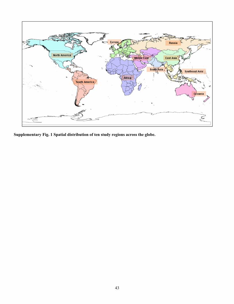
43

Supplementary Fig. 1 Spatial distribution of ten study regions across the globe.

44

Supplementary Fig. 2 Per capita N2O emission (kg N capita-1 yr-1) during 2007−2016. Annual population was obtained from FAOSTAT115 (http://www.fao.org/faostat/en/#data/OA).