Embed Size (px)
Citation preview
A comprehensive overview, behavioral model and
simulation of a Fault Current Limiter
Manish Verma
Thesis submitted to the faculty of the Virginia Polytechnic Institute and State University in partial fulfillment of the requirements for the degree of
Master of Science In
Electrical Engineering
Virgilio A. Centeno, Chair Yilu Liu
Jamie De La Ree
Keywords: Fault current, superconducting, PSCAD, solid state, hybrid, distribution system
Copyright© 2009, Manish Verma
June 29th, 2009 Blacksburg, Virginia
A comprehensive overview, behavioral model and simulation of a Fault Current Limiter
Manish Verma
Abstract Distribution systems across most parts of the globe are highly radial in nature. As loads
are gradually increased on a particular distribution system, a higher operating current state
leading to increased fault current levels is attained. Hence, the relay co-ordination is disturbed
and equipments such as feeders and circuit breakers need to be replaced with higher rating so
that they can handle the new currents often leading to expensive retrofit costs.
The use of fault current limiter (FCL) is proposed to mitigate the effects of high current
levels on a distribution system. A comprehensive and up-to-date literature review of FCL
technologies is presented. Detailed efforts of an in-house developed behavioral superconducting
FCL model are delineated, including FCL control algorithm and its implementation in
PSCAD®/EMTDC environment. Results from simulation studies are investigated and compared
to an actual FCL commissioned by Z-energy to highlight the effectiveness of a generic model
without having to access proprietary details. Extending those concepts, a solid-state and hybrid
type of limiter is also modeled and it results discussed. Finally, an impact assessment is
conducted on the distribution protection scheme, due to the FCL being inserted and subsequently
operated in the distribution system.

iii
Acknowledgements This thesis has been completed with utmost effort. Every detail has been taken care to
maintain a high level of accuracy and precision. First, I would like to thank my wonderful
advisor Dr. Virgilio Centeno for giving me the liberty to attack this work and for having the
determination to keep me focused on my thesis. Dr. Centeno’s assistance, encouragement and
financial support have been instrumental during my MS program at Virginia Tech. My interest in
power systems grew when I took my first introductory power course with Dr. Centeno during my
undergraduate years back in fall 2004. I’ll never forget his contribution to my career.
Dr. Jaime De La Ree and Dr. Yilu Liu served as my committee members, and were an
indispensable resource of information and ideas. The Center for Power Engineering faculty and
students helped create an enriching learning and fun environment. Classes and discussions with
Dr. Liu, Dr De Laree, Richard Cooper and others helped create the basis for my learning. All of
them are to be thanked as well.
This research was made possible from the generous grant provided by Southern
California Edison, on behalf of US Department of Energy. Much gratitude goes to Robert Yinger,
David Lubkeman and Dr. Mani S. Venkata without whose thoughtful advice; the research would
have been incomplete.
I would also like to thank Steve Peak, and Kathy Osbourn from TM GE Automation
Systems, Roanoke, VA for enabling me to take educational leave of absence from work and
pursue a higher degree.
Finally, I would like to thank god, my parents (Arti and Vipin Verma) and sister (Sonal)
for continued support, consideration and their persistent faith in me. Without their help, I would
have not been able to overcome the obstacles and move forward.
iv
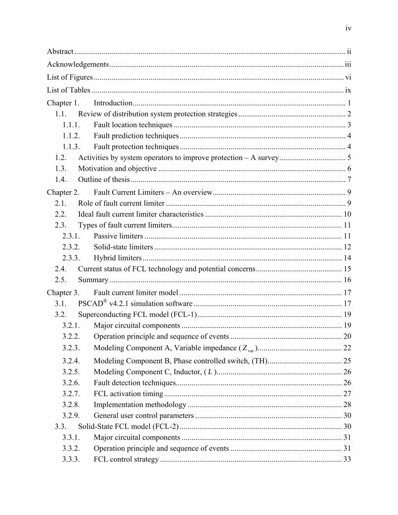
Abstract ........................................................................................................................................... ii
Acknowledgements........................................................................................................................ iii
List of Figures ................................................................................................................................ vi
List of Tables ................................................................................................................................. ix
Chapter 1. Introduction............................................................................................................. 1 1.1. Review of distribution system protection strategies ....................................................... 2
1.1.1. Fault location techniques ........................................................................................ 3 1.1.2. Fault prediction techniques ..................................................................................... 4 1.1.3. Fault protection techniques ..................................................................................... 4
1.2. Activities by system operators to improve protection – A survey.................................. 5 1.3. Motivation and objective ................................................................................................ 6 1.4. Outline of thesis .............................................................................................................. 7
Chapter 2. Fault Current Limiters – An overview.................................................................... 9 2.1. Role of fault current limiter ............................................................................................ 9 2.2. Ideal fault current limiter characteristics ...................................................................... 10 2.3. Types of fault current limiters....................................................................................... 11
2.3.1. Passive limiters ..................................................................................................... 11 2.3.2. Solid-state limiters ................................................................................................ 12 2.3.3. Hybrid limiters ...................................................................................................... 14
2.4. Current status of FCL technology and potential concerns............................................ 15 2.5. Summary ....................................................................................................................... 16
Chapter 3. Fault current limiter model ................................................................................... 17 3.1. PSCAD® v4.2.1 simulation software ............................................................................ 17 3.2. Superconducting FCL model (FCL-1).......................................................................... 19
3.2.1. Major circuital components .................................................................................. 19 3.2.2. Operation principle and sequence of events ......................................................... 20 3.2.3. Modeling Component A, Variable impedance ( )........................................... 22 varZ
3.2.4. Modeling Component B, Phase controlled switch, (TH)...................................... 25 3.2.5. Modeling Component C, Inductor, ( L )................................................................ 26 3.2.6. Fault detection techniques..................................................................................... 26 3.2.7. FCL activation timing ........................................................................................... 27 3.2.8. Implementation methodology ............................................................................... 28 3.2.9. General user control parameters ........................................................................... 30
3.3. Solid-State FCL model (FCL-2) ................................................................................... 30 3.3.1. Major circuital components .................................................................................. 31 3.3.2. Operation principle and sequence of events ......................................................... 31 3.3.3. FCL control strategy ............................................................................................. 33
v
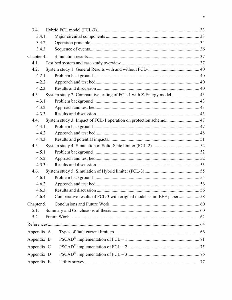
3.4. Hybrid FCL model (FCL-3).......................................................................................... 33 3.4.1. Major circuital components .................................................................................. 33 3.4.2. Operation principle ............................................................................................... 34 3.4.3. Sequence of events................................................................................................ 36
Chapter 4. Simulation results.................................................................................................. 37 4.1. Test bed system and case study overview..................................................................... 37 4.2. System study 1: General Results with and without FCL-1........................................... 40
4.2.1. Problem background ............................................................................................. 40 4.2.2. Approach and test bed........................................................................................... 40 4.2.3. Results and discussion .......................................................................................... 40
4.3. System study 2: Comparative testing of FCL-1 with Z-Energy model ........................ 43 4.3.1. Problem background ............................................................................................. 43 4.3.2. Approach and test bed........................................................................................... 43 4.3.3. Results and discussion .......................................................................................... 43
4.4. System study 3: Impact of FCL-1 operation on protection scheme.............................. 47 4.4.1. Problem background ............................................................................................. 47 4.4.2. Approach and test bed........................................................................................... 48 4.4.3. Results and potential impacts................................................................................ 51
4.5. System study 4: Simulation of Solid-State limiter (FCL-2) ......................................... 52 4.5.1. Problem background ............................................................................................. 52 4.5.2. Approach and test bed........................................................................................... 52 4.5.3. Results and discussion .......................................................................................... 53
4.6. System study 5: Simulation of Hybrid limiter (FCL-3)................................................ 55 4.6.1. Problem background ............................................................................................. 55 4.6.2. Approach and test bed........................................................................................... 56 4.6.3. Results and discussion .......................................................................................... 56 4.6.4. Comparative results of FCL-3 with original model as in IEEE paper.................. 58
Chapter 5. Conclusions and Future Work .............................................................................. 60 5.1. Summary and Conclusions of thesis ............................................................................. 60 5.2. Future Work .................................................................................................................. 62
References..................................................................................................................................... 64
Appendix: A Types of fault current limiters........................................................................... 66
Appendix: B PSCAD® implementation of FCL – 1............................................................... 71
Appendix: C PSCAD® implementation of FCL – 2............................................................... 75
Appendix: D PSCAD® implementation of FCL – 3............................................................... 76
Appendix: E Utility survey .................................................................................................... 77

vi
List of Figures Figure 1.1 PMU fault location method [3]...................................................................................... 3
Figure 2.1 Simple power circuit with and without FCL [9] ........................................................... 9
Figure 2.2 Series inductor application as a fault current limiter................................................... 11
Figure 2.3 Resonant type solid state limiter [10].......................................................................... 13
Figure 2.4 Triggered vacuum switch based hybrid limiter [12] ................................................... 14
Figure 2.5 Current and Voltage ratings for DOE sponsored projects [13] ................................... 15
Figure 3.1 PSCAD® v4.2.1 graphical user interface (GUI) [15] .................................................. 18
Figure 3.2 Superconducting fault current limiter (FCL-1) circuit diagram.................................. 20
Figure 3.3 FCL-1 sequence of events ........................................................................................... 21
Figure 3.4 FCL-1 component decomposition, per phase.............................................................. 22
Figure 3.5 Sequence of activation for variable impedance ................................................... 23 varZ
Figure 3.6 Third harmonic sinusoidal waveform.......................................................................... 25
Figure 3.7 Thyristor switch arrangement for harmonic injection ................................................. 26
Figure 3.8 FCL-1 activation timing diagram ................................................................................ 27
Figure 3.9 Line Current waveform before and during a fault....................................................... 29
Figure 3.10 IGCT-based half-controlled bridge FCL [18] ........................................................... 31
Figure 3.11 FCL-2 sequence of events [18].................................................................................. 32
Figure 3.12 LC resonance based hybrid FCL (FCL-3)................................................................. 34
Figure 3.13 Circuit for hybrid limiter (FCL-3) explanation [19].................................................. 34
Figure 4.1 Test bed radial distribution system used for FCL simulation...................................... 37
Figure 4.2 A typical radial distribution system used for FCL simulation .................................... 40
Figure 4.3 Phase A current waveform with and without FCL...................................................... 41
Figure 4.4 Phase A current RMS for with/without FCL............................................................... 41
Figure 4.5 Substation voltage with/without FCL.......................................................................... 42
Figure 4.6 Real power with/without FCL..................................................................................... 42
Figure 4.7 Line current waveform through (a) FCL-1, (b) Z-energy ........................................... 44
Figure 4.8 Line current RMS through (a) FCL-1, (b) Z-energy ................................................... 44
Figure 4.9 Line current waveform through (a) FCL-1, (b) Z-energy (Zoomed) .......................... 45
vii
Figure 4.10 Percent voltage drop pre-, during and post- fault for (a) FCL-1, (b) Z-energy......... 45
Figure 4.11 Line current with/without FCL-1 as fault distance increases.................................... 46
Figure 4.12 Percent reduction in current with FCL-1 as fault distance increases ........................ 47
Figure 4.13 A typical radial distribution system used for sectionalizer study.............................. 48
Figure 4.14 Recloser-Sectionalizer timing for fault beyond S4 ................................................... 49
Figure 4.15 Radial distribution system fault testing used for FCL simulation............................. 50
Figure 4.16 Test bed model for system study 4: Solid state model (FCL-2)................................ 53
Figure 4.17 Line current through FCL-2 for increasing impedances ........................................... 53
Figure 4.18 Line current waveform for (a) FCL-2, (b) FCL-1 ..................................................... 54
Figure 4.19 Voltage drop percentage comparison between FCL-1 and FCL-2............................ 55
Figure 4.20 Test bed model for system study 5: LC resonant model (FCL-3)............................. 56
Figure 4.21 Line current waveform for FCL-3............................................................................. 56
Figure 4.22 Line current through (a) FCL-3 and (b) FCL-1......................................................... 57
Figure 4.23 Rate of change of current for (a) FCL-3 and (b) FCL-1............................................ 58
Figure 4.24 Line current through (a) FCL-3 and (b) original model [19] .................................... 59
Figure 4.25 Voltage difference across FCL waveform (a) FCL-3 and (b) original model [19] ... 59
Figure A.1 Categories of Fault current limiter.............................................................................. 66
Figure A.2 Passive and Solid State limiters.................................................................................. 68
Figure A.3 Bridge type limiters .................................................................................................... 69
Figure A.4 Hybrid limiters............................................................................................................ 70
Figure B.1 PSCAD® FCL-1 Model (3-phase shown)................................................................... 71
Figure B.2 Fault detection control ................................................................................................ 72
Figure B.3 Simulation time extraction for impedance ramping ................................................... 72
Figure B.4 Variable impedance (Component A) ramping UP control ......................................... 72
Figure B.5 Variable impedance (Component A) ramping DOWN control .................................. 73
Figure B.6 Final reference to the variable impedance (Component A)........................................ 73
Figure B.7 Thyristor Firing Control (Courtesy: PSCAD®) .......................................................... 73
Figure B.8 Fault insertion control (Adapted from PSCAD® Master Library).............................. 74
Figure B.9 Sectionalizer control and coordination ....................................................................... 74
Figure C.1 PSCAD® FCL-2 Model (3-phase shown)................................................................... 75

viii
Figure C.2 Switch Firing Control (Courtesy PSCAD®) ............................................................... 75
Figure D.1 PSCAD® FCL-3 Model (3-phase, bold line indicates three phase)............................ 76
Figure D.2 Logic to monitor rate of change of current................................................................. 76
Figure D.3 Logic to monitor voltage waveforms.......................................................................... 76
Figure E.1 Table of industry survey responses............................................................................. 81
ix
List of Tables Table 3.1 Description of user control parameters for FCL-1........................................................ 30
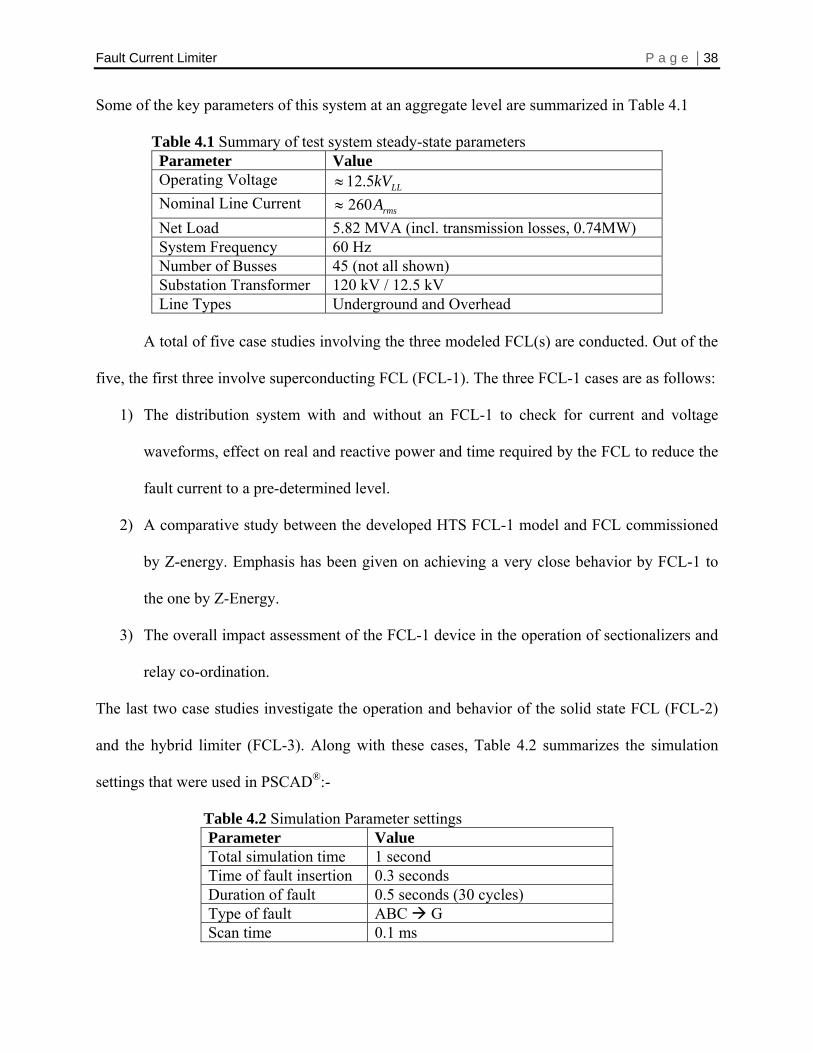
Table 4.1 Summary of test system steady-state parameters ......................................................... 38
Table 4.2 Simulation Parameter settings ...................................................................................... 38
Table 4.3 Line current values for fault at different distances from recloser................................. 39
Table 4.4 Line current with/without FCL-1 for fault at increasing distances from recloser ........ 46
Table 4.5 Sectionalizer/recloser settings....................................................................................... 50
Table 4.6 Sectionalizer/recloser operation.................................................................................... 51
Fault Current Limiter P a g e | 1
Chapter 1. INTRODUCTION Most, if not all of the devices that we use on a daily basis, utilize electrical power in some
way or another. As such, our lifestyles depend upon a reliable supply of electricity that is
available whenever we need it. Because our electrical supply is fairly reliable, it is assumed that
the lights will come on at the flip of a switch, that the refrigerator will keep food from spoiling,
and that the air conditioner will keep homes and offices comfortable.
The electricity that we use is typically supplied via a network of transmission lines that
carry the bulk of the power, and distribution lines that reach out to customer loads; like a house
or industry. The majority of the distribution systems in the United States operate in a radial
topology in which there is a single source of power that feeds the loads connected downstream
[1]. The topology is very simple to understand and their protection schemes are well understood
and work to protect loads and sources under fault conditions. However, over a period of years,
loads connected on a particular distribution system keeps increasing as new neighborhoods or
small industries are added to the system. This creates a situation where the normal operating
current increases, resulting in a proportional increase in the fault current levels. This may lead to
frequent power outages and ultimately customer dissatisfaction if corrective actions are not taken.
In order to operate within reliability and security constraints, an increase in current levels
necessitates two sizable modifications to the distributed system:
1) Retrofitting installed circuit breakers and feeders with higher rated equipment that can
handle the new fault current levels.
2) Re-configuration of protective devices with updated parameters.
In addition, with increased interest in distributed generation, sources like wind farms, solar
panels, fuel cells etc are being connected to the distribution system. The addition of sources to
Fault Current Limiter P a g e | 2 radial systems means that the current can now flow in either direction leading to massive and
costly overhauls of the protection system.
A Fault Current Limiter (FCL) is a revolutionary power system device that addresses the
problems due to increased fault current levels. As the name implies, a FCL is a device that
mitigates prospective fault currents to a lower manageable level. Building on this basis, the thesis
statement can be stated as follows:
“The appropriate approach to determine the feasibility of FCL technology is through the
development of flexible and faithful computer-aided models and then applying them in a
distribution system environment to analyze their performance, effects and practical
realization.”
Following from the thesis statement, the work in this thesis makes two major contributions. First,
a consolidated and up-to-date literature study of a wide variety of the FCL(s) that have been
researched, prototyped and field tested. Second, the development of FCL models for the
computer aided design software called PSCAD® that can be used for network studies and
modified to accommodate other kinds of FCL(s) to distribution systems.
1.1. Review of distribution system protection strategies Fault location, prediction, and protection are the most important aspects of fault
management for the reduction of outage time. In the past, most of the research and development
on power system faults in these areas has focused on transmission systems, and it is not until
recently with deregulation and competition, that research on power system faults has begun to
focus on the unique aspects of distribution systems [2] . Below is a brief overview of some of the
techniques used or proposed for fault location, prediction and protection.
Fault Current Limiter P a g e | 3
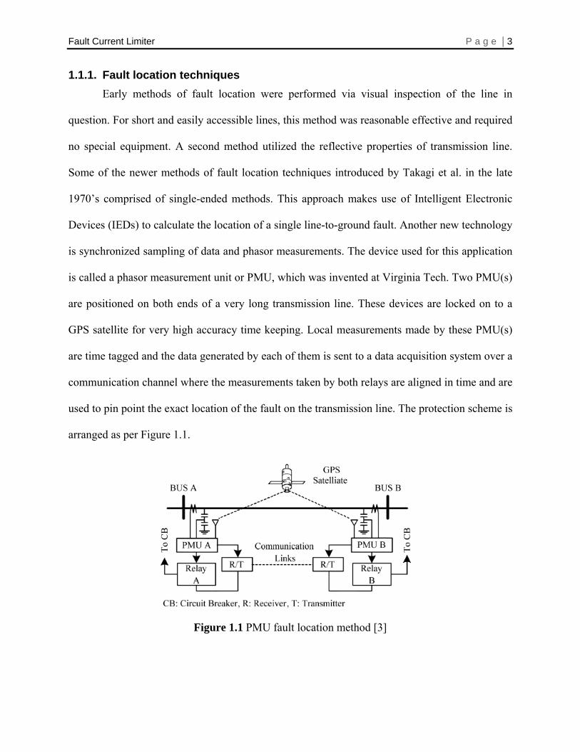
1.1.1. Fault location techniques Early methods of fault location were performed via visual inspection of the line in
question. For short and easily accessible lines, this method was reasonable effective and required
no special equipment. A second method utilized the reflective properties of transmission line.
Some of the newer methods of fault location techniques introduced by Takagi et al. in the late
1970’s comprised of single-ended methods. This approach makes use of Intelligent Electronic
Devices (IEDs) to calculate the location of a single line-to-ground fault. Another new technology
is synchronized sampling of data and phasor measurements. The device used for this application
is called a phasor measurement unit or PMU, which was invented at Virginia Tech. Two PMU(s)
are positioned on both ends of a very long transmission line. These devices are locked on to a
GPS satellite for very high accuracy time keeping. Local measurements made by these PMU(s)
are time tagged and the data generated by each of them is sent to a data acquisition system over a
communication channel where the measurements taken by both relays are aligned in time and are
used to pin point the exact location of the fault on the transmission line. The protection scheme is
arranged as per Figure 1.1.
Figure 1.1 PMU fault location method [3]
Fault Current Limiter P a g e | 4
1.1.2. Fault prediction techniques The intent of fault prediction is to determine a failure in a system component early
enough to allow for maintenance or replacement of the suspected component. Fault prediction
can be divided into early detection techniques, data mining, and hidden failures.
A large portion of the research into early detection techniques concentrates on thermal
analysis and other non-invasive techniques for the early detection of damaged components such
as transformers, fault arresters, and insulators [2]. Microprocessor based control, automation and
instrumentation has allowed us to capture voltage and current measurements, to name a few,
before, during and after the fault. This combined with high speed communications and storage
media, makes the availability of large fault databases on which statistical data mining approach
is used to analyze and address the cause of distribution faults [2]. Hidden failures in protection
systems have been identified as key contributors in the cascading of power system wide-area
disturbances [4]. Although, primarily developed for transmission systems, these concepts may
also be applicable to preventing the spread of distribution systems faults.
1.1.3. Fault protection techniques Fault protection of distribution faults is a mature subject and has been well understood.
Some of the advanced techniques of fault protection are distributed automation, detecting high
impedance faults and fault current limiters [2]. The most common automated functions in
distribution systems include the following: Volt/Var Control, Fault Location Isolation and
Service Restoration (FLIR), Optimal Feeder Reconfiguration, Automated Meter Reading, and
Relay Protection Re-coordination [2]. High impedance faults is defined by IEEE PSRC working
group as those that “do not produce enough fault current to be detected by conventional over-
current relays or fuses” [5]. This is a relatively recent subject of interest where very few facilities
Fault Current Limiter P a g e | 5 exist to test for high impedance faults. Fault current limiters, as already mentioned before are
finding increased use in distribution system protection.
1.2. Activities by system operators to improve protection – A survey A short survey was carried out as a part of the research project of fault current limiters.
Questions related to the current strategies for distribution protection, adaptive protection using
automation and high end computing were asked to distribution system engineers. Also,
communication topologies, advanced data management and processing, and types of sensors
used were also queried as a part of the survey. About a dozen companies, most of them utilities,
responded to the survey [Appendix E]. Below is a snapshot of the responses:
In order to carry out fault protection, most of the companies are using advanced
decentralized systems that monitors a particular section and reports to a central database. Each
system acts as a child of the overall system (parent) which has built-in intelligence to take
necessary corrective action without human interaction. A company reports that they have
recently installed Feeder Automation System Technology (FAST), which is an intelligent
switching mechanism that will restore power in the event of an outage. Others are developing in-
house protection scheme such as Remedial Action Scheme (RAS) for back up power supplies
and Overload Scheme (OLS) for grid protection. Also, specific hardware and software
technologies are being deployed that measure the performance of transformers, circuit breakers,
and other components for efficient utilization of assets and predict failure. Reliability statistical
analysis data about customer outages is being used to feed into an indigenously developed
application that can take corrective action.
With the advent of reliable fiber-optic technology, many companies have started to
retrofit their existing system with fiber. These cables are installed along with the power
Fault Current Limiter P a g e | 6 conductors and in power duct banks to transmit real-time temperature for dynamic ratings and
increased asset utilization. Fiber optic voltage and current sensors are also being used, which
have a better precision and are also portable to a certain extent. Utilities have also installed
numerous smart meters at strategic locations to better predict an outage size and location based
on historical trends stored within these meters. These smart meters can also communicate fault
location faster than the traditional “call-in” method. Besides the above mentioned, utilities have
also discussed their plans on testing fault current limiter technology in the near future.
1.3. Motivation and objective The current trend in distribution systems is pointing towards more sophisticated and
intelligent ways of protection without jeopardizing system stability and maintaining continuous
power supply to customers. The current “New Energy for America” plan calls for 10% of
electricity to come from renewable sources by 2010 and 25% by 2025 [6]. This power will
mostly be fed in the form of distributed generation. As stated before, distributed generation
injects additional current to the system under fault, which cannot be handled by existing
protection schemes.
The motivation arises with the fact that “as the deregulation environment takes hold and
utilities seek more efficient and cost-effective methods to couple grids, improve power quality,
and delay expensive upgrades,” [7] fault current limiters will find increased application in
distribution systems. Currently, researchers have been experimenting with various FCL
technologies strictly via computer simulation that is very specific in nature. Power companies
have also started investing in this technology as they see immense potential in current limiting
technologies.
Fault Current Limiter P a g e | 7
The objective of this thesis is to create a flexible FCL model for PSCAD® based on the
most promising technologies that can be used for fault and system analysis. PSCAD® is
graphical user interface based power system software that allows for detailed modeling of
transmission, distribution systems, machines etc and is widely used in the industry. It is the
author’s hope that this work will be beneficial to power engineers when considering installing a
fault current limiter in their particular system.
1.4. Outline of thesis The subsequent content is structured as follows:
Chapter 2, Fault current limiters – An Overview, reviews the role of an FCL and the
need for it. A comprehensive table summarizes some of the different categories and the most
promising types of FCL, explaining the method of operation along with references. A brief
summary of the current status of the FCL technology and potential concerns have also been
addressed.
Chapter 3, FCL model, presents a practical approach to a computer aided model using
industry standard PSCAD® software. Special emphasis is given to modeling a superconducting
FCL, outlining the operation principle, fault detection and activation algorithms. Solid-state and
hybrid limiters are also modeled and some of the techniques involved with them.
Chapter 4, Simulation results, presents the findings of the FCL models under a test
distribution system. Comparisons of an in-house developed superconducting fault current limiter
(SFCL) are made against the results obtained by the SFCL from Z-energy. Short case studies are
conducted on the test distribution system to check for FCL performance and assess its overall
impact on the protection scheme. Results of solid-state limiter and hybrid limiters are also
studied.
Fault Current Limiter P a g e | 8
Chapter 5, Conclusions and Future Work, summarizes the work done, along with some
of the major contributions that this thesis makes in the field of fault current limiters. A brief
recommendation of prospective future direction is also delineated.
Fault Current Limiter P a g e | 9
Chapter 2. FAULT CURRENT LIMITERS – AN OVERVIEW Damage from short circuit currents is a constant threat to any electric power system,
since it threatens the integrity of its generators, bus-bars, transformers, switchgears, and
transmission and distribution lines [8]. Building on this statement, the FCL is described below.
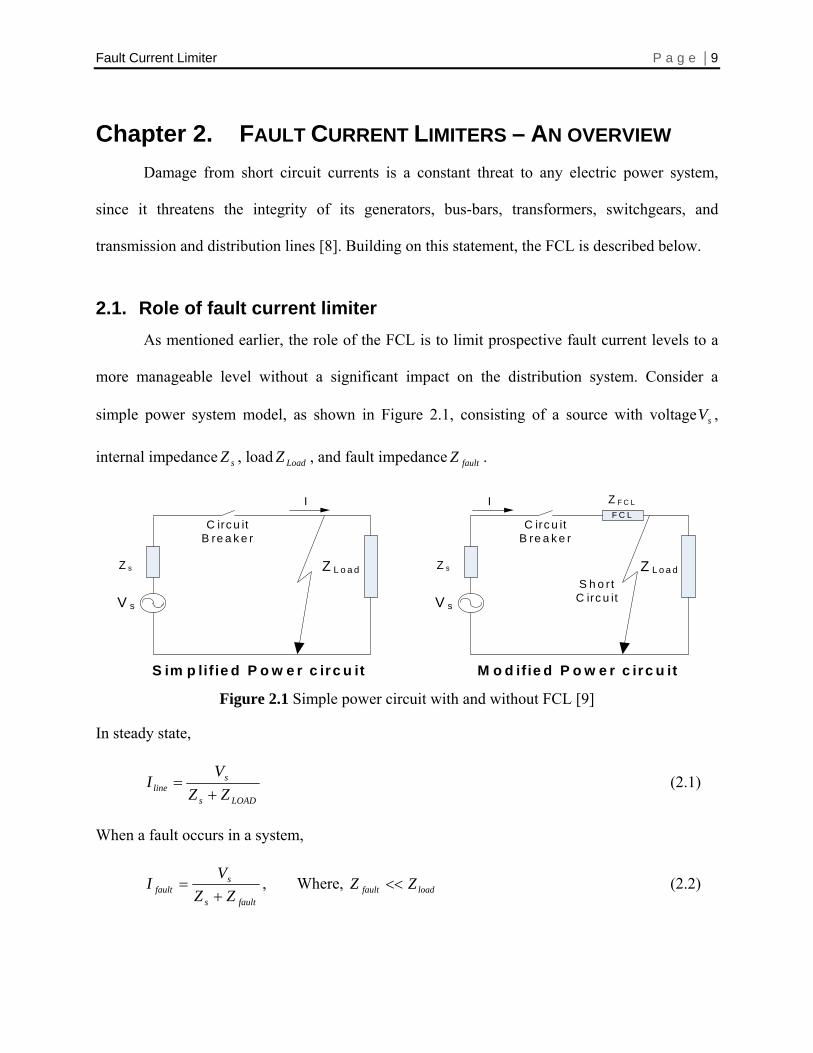
2.1. Role of fault current limiter As mentioned earlier, the role of the FCL is to limit prospective fault current levels to a
more manageable level without a significant impact on the distribution system. Consider a
simple power system model, as shown in Figure 2.1, consisting of a source with voltage ,
internal impedance , load , and fault impedance .
sV
sZ LoadZ faultZ
V s
Z s Z L o a d
I
C irc u it B re a k e r
V s
Z s
I
C irc u it B re a k e r
F C L
Z F C L
S h o r t C irc u it
S im p lif ie d P o w e r c irc u it M o d if ie d P o w e r c irc u it
Z L o a d
Figure 2.1 Simple power circuit with and without FCL [9]
In steady state,
LOADs
sline ZZ
VI
+= (2.1)
When a fault occurs in a system,
faults
sfault ZZ
VI
+= , Where, loadfault ZZ << (2.2)
Fault Current Limiter P a g e | 10
Since the supply impedance is much smaller than the load impedance, Equation (2.2) shows
that the short circuiting of the load will substantially increase the current flow. However, if a
FCL is placed in series, as shown in the modified circuit, Equation (2.3) will hold true;
sZ
faultFCLs
sfault ZZZ
VI
++= (2.3)
Equation (2.3) tells that, with an insertion of a FCL, the fault current will now be a function of
not only the source and fault impedance , but also the impedance of the FCL. Hence, for
a given source voltage and increasing will decrease the fault current .
sZ faultZ
FCLZ faultI
2.2. Ideal fault current limiter characteristics Before discussing any further, it is important that some of the ideal characteristics be laid
out for an FCL. An ideal FCL should meet the following operational requirements [1, 7, 10, 11]:-
1) Virtually inexistent during steady state. This implies almost zero voltage drop across the
FCL itself
2) Detection of the fault current within the first cycle (less than 16.667ms for 60Hz and
20ms for 50Hz) and reduction to a desirable percentage in the next few cycles.
3) Capable of repeated operations for multiple faults in a short period of time
4) Automatic recovery of the FCL to pre-fault state without human intervention
5) No impact on voltage and angle stability
6) Ability to work up to the distribution voltage level class
7) No impact on the normal operation of relays and circuit breakers
8) Finally, small-size device that is relatively portable, lightweight and maintenance free
In reality, one would like to have an FCL that would satisfy all of the foregoing characteristics.
However, certain trade-offs and compromises have been made in nearly all categories and types.
Fault Current Limiter P a g e | 11
2.3. Types of fault current limiters This section presents a brief review of the various kinds of FCL that has been
implemented or proposed. FCL(s) can generally be categorized into three broad types:
1) Passive limiters
2) Solid state type limiters, and
3) Hybrid limiters
In the past, many approaches to the FCL design have been conducted ranging from the very
simple to complex designs. A brief description of each category of limiter is given below.
Appendix A of this thesis has a consolidated and more detailed list of the different FCL types.
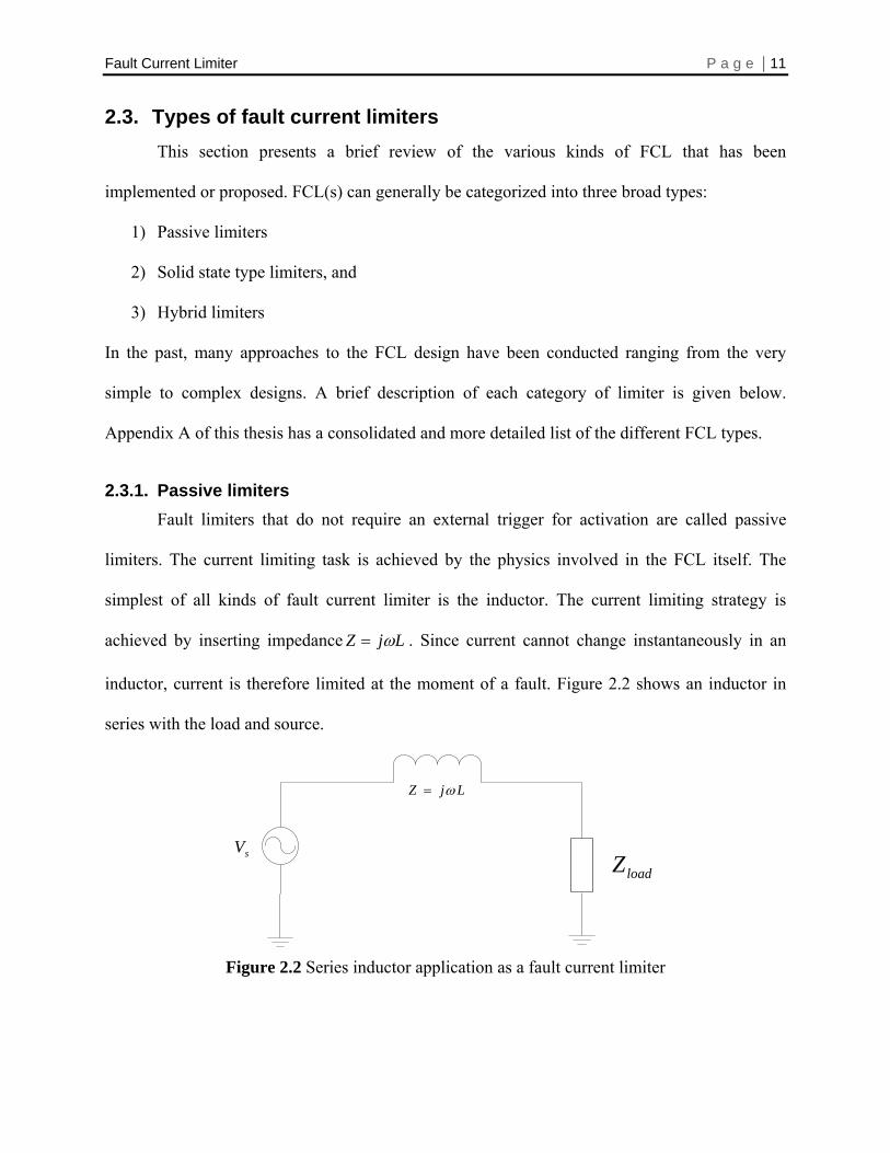
2.3.1. Passive limiters Fault limiters that do not require an external trigger for activation are called passive
limiters. The current limiting task is achieved by the physics involved in the FCL itself. The
simplest of all kinds of fault current limiter is the inductor. The current limiting strategy is
achieved by inserting impedance LjZ ω= . Since current cannot change instantaneously in an
inductor, current is therefore limited at the moment of a fault. Figure 2.2 shows an inductor in
series with the load and source.
LjZ ω=
sVloadZ
Figure 2.2 Series inductor application as a fault current limiter
Fault Current Limiter P a g e | 12 There are a few pros and cons in using an inductor for FCL application:
1) Technique has been well known, installed, field tested and commissioned for many years
2) Relatively low cost and maintenance, but
3) Bulky to handle and replace
4) Produces a voltage drop in steady state and causes lagging power factors
Another kind of passive limiter that is gaining attention is the super conducting fault
current limiter (SFCL). Superconductor materials lose their electrical resistance below certain
critical values of temperature, magnetic field, and current density [8]. SFCL(s) work on the
principle that under steady state, it allows for the load current to flow through it without
appreciable voltage drop across it. During a fault, an increase in the current leads to a
temperature rise and a sharp increase in the impedance of the superconducting material. SFCL(s)
are discussed in greater detail in Chapter 3 and 4. Below are a few advantages and disadvantages
of using an SFCL:
1) Virtually no voltage drop in steady state
2) Quick response times and effective current limiting, but
3) Cooling technologies still at infancy, leading to frequent break downs
4) Commercial deployment is still to be witnessed
5) Superconducting coils can saturate and lead to harmonics
2.3.2. Solid-state limiters Recent developments in power switching technology have made solid state limiters
suitable for voltage and power levels necessary for distribution system applications. Solid state
limiters use a combination of inductors, capacitors and thyristors or gate turn off thyristors
(GTO) to achieve fault limiting functionality.
Fault Current Limiter P a g e | 13
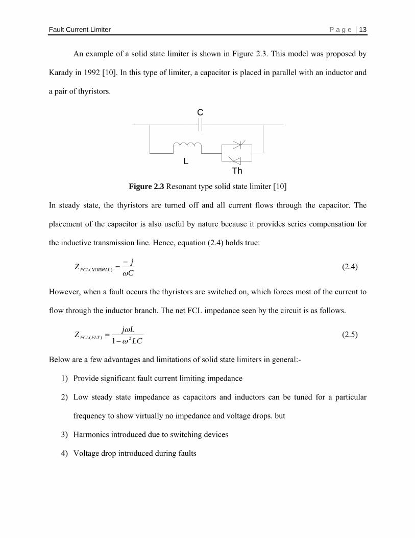
An example of a solid state limiter is shown in Figure 2.3. This model was proposed by
Karady in 1992 [10]. In this type of limiter, a capacitor is placed in parallel with an inductor and
a pair of thyristors.
C
LTh
Figure 2.3 Resonant type solid state limiter [10] In steady state, the thyristors are turned off and all current flows through the capacitor. The
placement of the capacitor is also useful by nature because it provides series compensation for
the inductive transmission line. Hence, equation (2.4) holds true:
CjZ NORMALFCL ω
−=)( (2.4)
However, when a fault occurs the thyristors are switched on, which forces most of the current to
flow through the inductor branch. The net FCL impedance seen by the circuit is as follows.
LCLjZ FLTFCL 2)( 1 ω
ω−
= (2.5)
Below are a few advantages and limitations of solid state limiters in general:-
1) Provide significant fault current limiting impedance
2) Low steady state impedance as capacitors and inductors can be tuned for a particular
frequency to show virtually no impedance and voltage drops. but
3) Harmonics introduced due to switching devices
4) Voltage drop introduced during faults
Fault Current Limiter P a g e | 14
2.3.3. Hybrid limiters As the name implies, hybrid limiters use a combination of mechanical switches, solid
state FCL(s), superconducting and other technologies to create current mitigation. It is a well
know fact that circuit breakers and mechanical based switches suffer from delays in the few
cycles range. Power electronic switches are fast in response and can open during a zero voltage
crossing hence commutating the voltage across its contacts in a cycle [1].
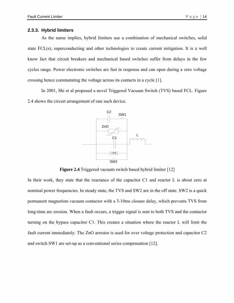
In 2001, Shi et al proposed a novel Triggered Vacuum Switch (TVS) based FCL. Figure
2.4 shows the circuit arrangement of one such device.
TVS
C2
C1
ZnO
SW2
SW1
L
Figure 2.4 Triggered vacuum switch based hybrid limiter [12]
In their work, they state that the reactance of the capacitor C1 and reactor L is about zero at
nominal power frequencies. In steady state, the TVS and SW2 are in the off state. SW2 is a quick
permanent magnetism vacuum contactor with a 3-10ms closure delay, which prevents TVS from
long-time arc erosion. When a fault occurs, a trigger signal is sent to both TVS and the contactor
turning on the bypass capacitor C1. This creates a situation where the reactor L will limit the
fault current immediately. The ZnO arrestor is used for over voltage protection and capacitor C2
and switch SW1 are set-up as a conventional series compensation [12].
Fault Current Limiter P a g e | 15
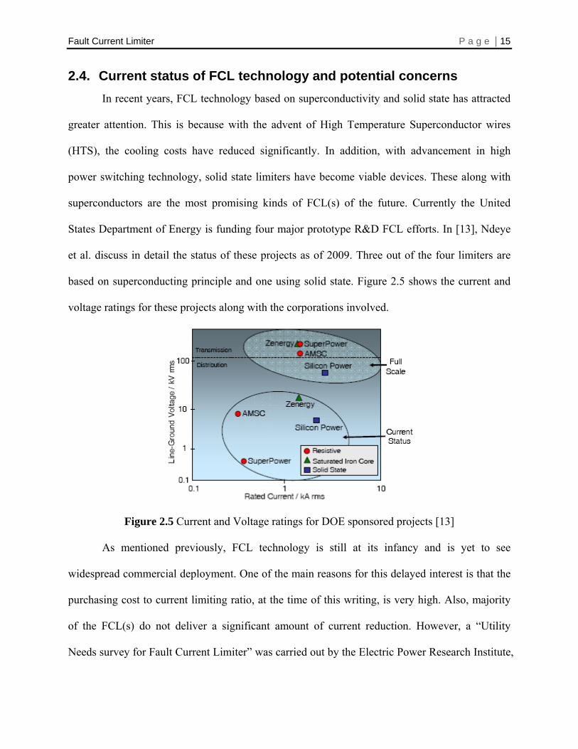
2.4. Current status of FCL technology and potential concerns In recent years, FCL technology based on superconductivity and solid state has attracted
greater attention. This is because with the advent of High Temperature Superconductor wires
(HTS), the cooling costs have reduced significantly. In addition, with advancement in high
power switching technology, solid state limiters have become viable devices. These along with
superconductors are the most promising kinds of FCL(s) of the future. Currently the United
States Department of Energy is funding four major prototype R&D FCL efforts. In [13], Ndeye
et al. discuss in detail the status of these projects as of 2009. Three out of the four limiters are
based on superconducting principle and one using solid state. Figure 2.5 shows the current and
voltage ratings for these projects along with the corporations involved.
Figure 2.5 Current and Voltage ratings for DOE sponsored projects [13]
As mentioned previously, FCL technology is still at its infancy and is yet to see
widespread commercial deployment. One of the main reasons for this delayed interest is that the
purchasing cost to current limiting ratio, at the time of this writing, is very high. Also, majority
of the FCL(s) do not deliver a significant amount of current reduction. However, a “Utility
Needs survey for Fault Current Limiter” was carried out by the Electric Power Research Institute,
Fault Current Limiter P a g e | 16 EPRI in 2008. In his presentation [14], Eckroad reports that potential market for FCL technology
is about two FCLs per utility per year. This is based on the assumption that FCL is the most cost
effective way to manage fault currents. He also mentions that roughly 50% of the potential
customers would accept two to five times the cost of a novel FCL over a circuit breaker.
However, the cost of ownership and fail safe design are the fundamental features that all
customers would like to see in an FCL so that their investments are justified [14]. Also, “one of
the delays to the faster adoption of FCLs is that there are currently no standardized testing
protocols in place to test them,”[13]. There are very few test facilities across the globe that
provides a one-stop place to test out the FCLs. For instance, liquid nitrogen for cooling is
required in testing some superconducting types of FCLs. It is very hard to find facilities that
provide advance cooling apparatus along with high voltage and power. International partnerships
and scholars are helping pave the way to a more streamlined testing standards, procedures and
facilities.
2.5. Summary In this chapter, the role of the FCL and some of the ideal characteristics of an FCL model
were discussed. Also a brief overview of the various kinds of FCL(s) was given along with their
respective advantages and disadvantages. A much more detailed literature review can be found in
Appendix A. A summary of the current status of FCL(s) and potential concerns with testing out
this technology has also been addressed.
Based on the trends reviewed for FCL, it is a ripe time to model various FCL(s). Chapter
3 will show in detail the process of modeling a superconducting, solid-state and hybrid limiter in
PSCAD®/EMTDC software along with the results of the simulation and test cases in Chapter 4.
Fault Current Limiter P a g e | 17
Chapter 3. FAULT CURRENT LIMITER MODEL Computer-aided modeling and simulation of any physical device or phenomena is
perhaps one of the most fundamental practices in power system studies. In this chapter, a
PSCAD® model for a superconducting, solid state and hybrid type of fault current limiter is
proposed and its implementation process is presented. The proposed FCL is a behavioral model
whose sole aim is to simulate the operation of a real device without the need of proprietary
parameters and functional descriptions from the manufacturers. In summary, the developed
PSCAD® model requires only a handful of input parameters for which the user has complete
control.
3.1. PSCAD® v4.2.1 simulation software To study the effects of a FCL model, simulation software is chosen as a preferred
investigative means rather than a physical system testing which is more time consuming and
expensive. The use of simulation software allows for a quick and easy way to model FCL(s) and
to test their effect in a distribution system. PSCAD® version 4.2.1 is industry leading, powerful
and flexible power systems software. It uses the world renowned EMTDC solution engine that
enables for simulating the time domain instantaneous responses (electromagnetic transients) of
electrical systems. PSCAD allows the user to graphically assemble the circuit, run the simulation,
and analyze the results. PSCAD comes complete with a library of pre-programmed and tested
models, ranging from simple passive elements and control functions, to more complex models,
such as electric machines, FACTS devices, transmission lines and cables that can be dragged-
and-dropped to create systems and obtain accurate responses [15]. Furthermore, PSCAD also
allows the user to create custom blocks by combining basic elements along with control
Fault Current Limiter P a g e | 18 functions. This is especially useful for our study as it will enable us to model the FCL more
realistically and to package it in a single block of code with a set number of user input and output
functions. Following are a few case studies that are typically conducted on PSCAD® [15]:-
• Contingency studies of AC networks consisting of machines, exciters, governors etc
• Relay coordination
• Transformer saturation effects
• Evaluation of filter design and harmonic analysis
• Control system design and coordination of FACTS and HVDC
• Optimal design of controller parameters
• Investigation of new circuit and control concepts
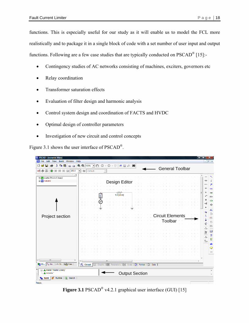
Figure 3.1 shows the user interface of PSCAD®.
Design Editor
Project section Circuit Elements Toolbar
Output Section
General Toolbar
Figure 3.1 PSCAD® v4.2.1 graphical user interface (GUI) [15]
Fault Current Limiter P a g e | 19 The workspace can be divided into three sections. The “Project section” lists all the loaded cases
and libraries. The “Output section” shows the status of each project and any errors or warnings
that the project might have. The “Design editor” section consists of the actual circuit diagram
that is under investigation. The “Circuit element toolbar” provides an easy drag-and-drop feature
to insert circuit elements, although a larger selection is available via the master library. The
“General Toolbar” consists of standard Windows® features like cut, copy, paste, zoom etc. All of
these features provide for a very user oriented interface that is easy and fun to work with.
3.2. Superconducting FCL model (FCL-1) As mentioned previously, SFCL is one of the most promising type of limiter and has the
greatest potential. A detailed time domain model of the SFCL is proposed and implemented, here
after referred as FCL-1. Details such as major FCL components, operation principles and
sequence of events, fault detection techniques, and timing diagrams are presented.
3.2.1. Major circuital components The first model created is a saturated core high temperature superconducting (HTS) type
fault current limiter. High temperature superconductors are cooled to a much higher temperature
that conventional superconductors hence saving significant space and costs in cooling apparatus.
This is the same model as conceptualized by Z-energy, but using different components and
developed in-house. In principle, the saturated core FCL utilizes larger differences in the
permeability of magnetic material. Fundamentally, high permeability materials allow for a low
impedance during normal operation and a very high impedance during fault current levels [16].
However, from a modeling standpoint, FCL-1 can be modeled as a combination of inductor
wound with superconducting HTS wire, thyristor and variable resistor. This arrangement is
shown below in Figure 3.2.
Fault Current Limiter P a g e | 20
LTh
LTh
LTh
LineI
LineI
Normal State:
Faulted State:
varZ
)(0var ShortZ Ω=
)(106var OpenZ Ω=
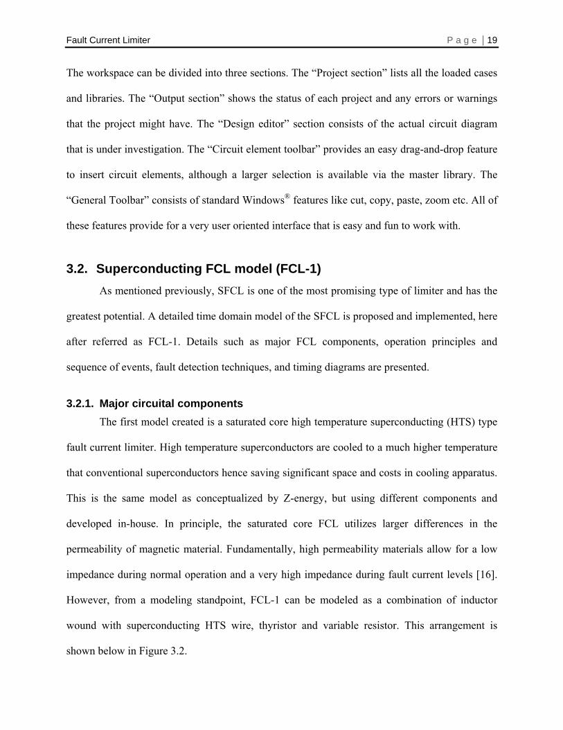
Figure 3.2 Superconducting fault current limiter (FCL-1) circuit diagram The significance of each of the components is as follows:-
1) The inductor is wound with a HTS superconducting wire that is cooled by a separate
cooling apparatus. Upon a high fault current, the impedance of the wire increases sharply
with time and temperature hence providing the current limiting feature. Also, since
current cannot change instantaneously in an inductor, it provides an effective way of
mitigating high currents within the first cycle.
2) The thyristor is inserted to closely model the harmonic component in the FCL operation.
This is crucial to model as other power system components might have adverse effect due
to harmonics.
3) Linear variable impedance is employed to model the opening of a mechanical switch and
the arc voltage produced by it.
3.2.2. Operation principle and sequence of events The basic idea of any super conducting fault current limiter (SFCL), is as follows,
1) At faultTt < , the impedance of the SFCL is close to 0Ω
Fault Current Limiter P a g e | 21
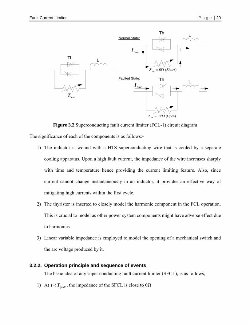
2) At faultTt > , the impedance of the SFCL rises sharply within a few milliseconds.
Consider the FCL-1 circuit diagram in Figure 3.3 reproduced from Figure 3.2. The sequence of
events is as follows:-
LTh
varZPath A
Path B
Figure 3.3 FCL-1 sequence of events
1) For time faultTt < , the thyristors (TH) are switched off and the variable impedance varZ is
close to 0Ω . All the line current flows through the resistor and the inductor as per “Path
A”. Since the inductor is wound with a HTS wire, there is no significant line impedance
and the voltage drop is very negligible, (<1%)
2) At time faultTt = , a bolted three phase-to-ground fault is inserted right at the terminals of
the FCL on the load side.
3) At time ms , the thyristors are fired and varZ is sharply increased to simulate
the opening of a switch and the arc voltage produced by it.
Tt fault 100+=
4) At time ms , all the current is now commutated through the thyristor and the
inductor. The current is mitigated and flows as per “Path B”.
Tt fault 150+=
5) For time duration , the fault is kept inserted in the system faultTt fault +≥
6) At time faultclearTt , the fault is removed and the impedance of resistor is ramped down to
0Ω and the thyristors are switched off, commutating the current through “Path A”.
=

Fault Current Limiter P a g e | 22
7) At time faultclearTt , the FCL comes back to the steady operating state >>
From a simulation standpoint, the important aspect to develop is the automatic fault detection
algorithm and correct reaction by the SFCL to mitigate the effects of dangerous fault currents.
By automatic detection, we mean that there is no external trigger or relay to the SFCL to start its
operation. The triggering of SFCL is purely a function of the line quantities and its appropriate
manipulation to predict a fault situation. This was briefly discussed in section 2.3.1.
In the following section, the actual implementation of the modeling efforts is presented.
First, let us decompose the FCL model into three components A, B, and C respectively as shown
in Figure 3.4
LTh
A
B C
varZ
Figure 3.4 FCL-1 component decomposition, per phase
3.2.3. Modeling Component A, Variable impedance ( varZ )
Component A in Figure 3.4 consists of a variable impedance that is at 0Ω (short circuit)
at steady state. When a fault occurs, the impedance is quickly increased simulating the opening
of a switch at the rate of 100 - 200Ω /s (user settable). Accurate modeling of this component is
critical as ramp reference to this component will be given ONLY after it is annunciated that a
fault does exist in the system and subsequently an action is to be taken.
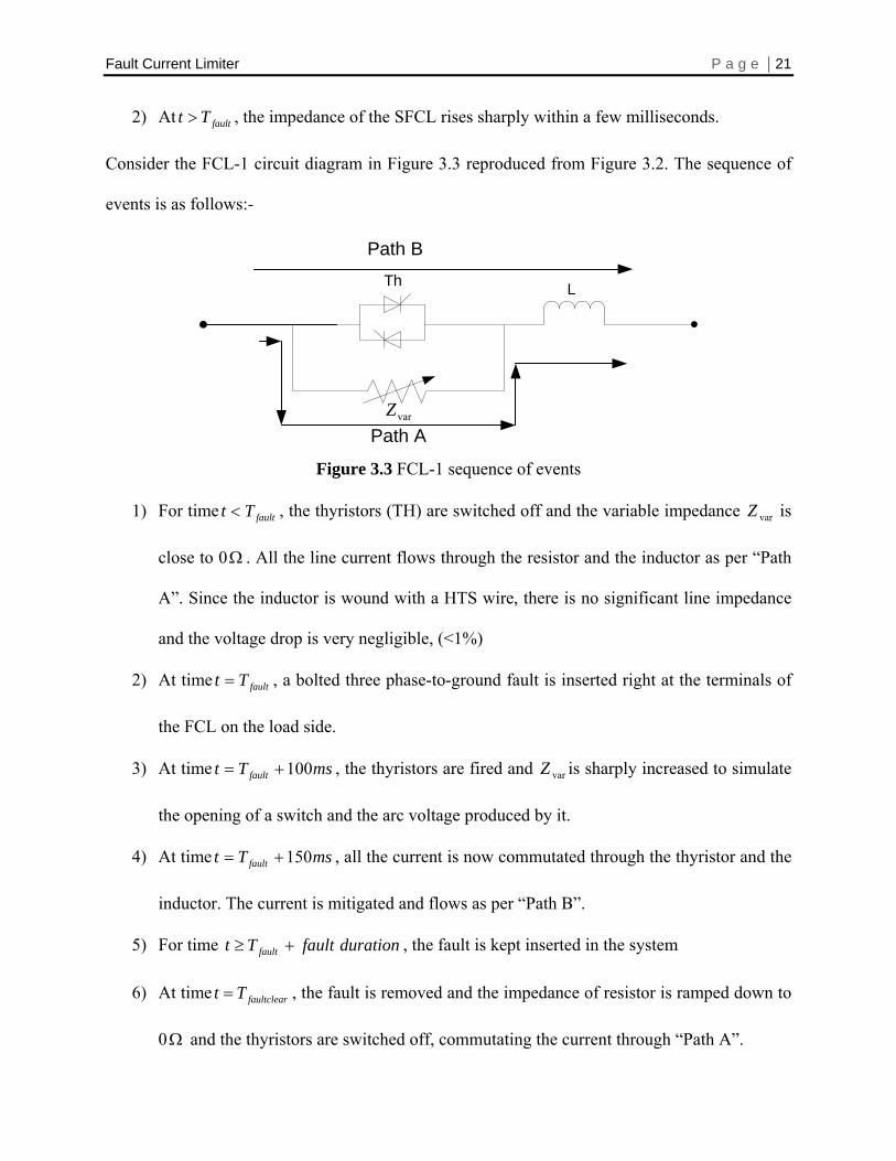
The sequence of operation of this variable resistor is shown in Figure 3.5. A description
is also given following the flowchart.
Fault Current Limiter P a g e | 23
Start
Initialize
)/(&10 6
sZZ
slope
initial
ΩΩ= −
dtdiMonitor IAND
IF
for > TD-1alNoI min>
IF alNo
dtdi min>
Wait for TD-2 ms and then Trigger RAMP
Start Impedance ramping UP at
)/( sZslope Ω
YES
NO
YES
Stop
IF alNo
dtdi min<
Reach Maximum Impedance limit
Wait for TD-3 ms and then Start Impedance ramping DOWN at
NO
Yes
NO
)/( sZslope Ω
)(max ΩZ
)/( sZslope Ω
)(max ΩZ
User Control Parameters:
- Rate at which to ramp up impedance- Maximum impedance of resistor- Nominal line current
TD-1/2/3 (sec) - Time delays(can be 0 seconds)
Nominal (A)
Figure 3.5 Sequence of activation for variable impedance varZ
Fault Current Limiter P a g e | 24
Before starting the simulation, the resistor is initialized with an initial impedance value
and a ramp rate . The simulation is then started where the current magnitude
and the rate of change of current is monitored during the entire simulation time. After achieving
some steady state operating point a three phase-to-ground fault is inserted into the system
external to the FCL. As soon as the fault is inserted, the magnitude of the line current jumps up
instantaneously and achieves a new steady state value as long as the fault is present. However, in
order to make sure that there is indeed a fault in the distribution system and that the impedance is
not falsely triggered, the rate of change of current is also monitored. A fault will change the rate
instantaneously. After setting the necessary flags, the impedance is ramped up at a rate
)(ΩinitialZ )(ΩslopeZ
)(ΩslopeZ
As long as the fault is present, the impedance will keep increasing till a maximum value )(max ΩZ .
After the fault is cleared the impedance will be ramped down to the initial impedance. This cycle
takes place whenever there is a fault.
Typically in industrial automation and control, a time delay (TD) is added before any
action is taken. This is especially true if the action to be taken is dependent on inputs from
sensors, limit switches, proximity switches, etc. By doing so, momentary switching which would
otherwise trigger an action is eliminated. Similar concepts can also be applied to a power
protection. Many times, faults come and go at an instant. This might happen because of a tree
touching the line due to windy weather or a squirrel trying to jump between lines or even
momentary in-rush currents due to a heavy load coming online. Hence, the goal would be to
trigger the FCL only after making sure that there is indeed a fault. This is possible by inserting a
delay timer. Appropriate delay times can be 2 to 3 cycles or more. A similar delay timer can be
used when switching off the FCL. This is done by making sure that the fault has been cleared
before the FCL impedance is ramped down.
Fault Current Limiter P a g e | 25
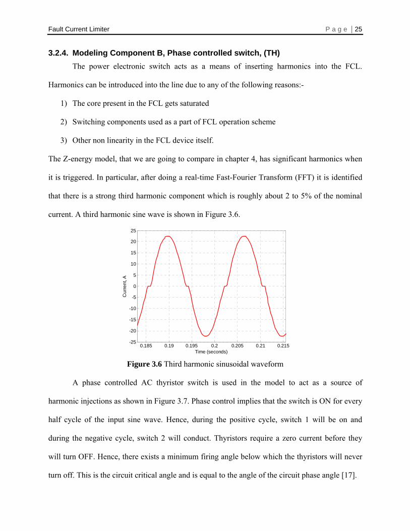
3.2.4. Modeling Component B, Phase controlled switch, (TH) The power electronic switch acts as a means of inserting harmonics into the FCL.
Harmonics can be introduced into the line due to any of the following reasons:-
1) The core present in the FCL gets saturated
2) Switching components used as a part of FCL operation scheme
3) Other non linearity in the FCL device itself.
The Z-energy model, that we are going to compare in chapter 4, has significant harmonics when
it is triggered. In particular, after doing a real-time Fast-Fourier Transform (FFT) it is identified
that there is a strong third harmonic component which is roughly about 2 to 5% of the nominal
current. A third harmonic sine wave is shown in Figure 3.6.
0.185 0.19 0.195 0.2 0.205 0.21 0.215-25
-20
-15
-10
-5
0
5
10
15
20
25
Time (seconds)
Cur
rent
, A
Figure 3.6 Third harmonic sinusoidal waveform
A phase controlled AC thyristor switch is used in the model to act as a source of
harmonic injections as shown in Figure 3.7. Phase control implies that the switch is ON for every
half cycle of the input sine wave. Hence, during the positive cycle, switch 1 will be on and
during the negative cycle, switch 2 will conduct. Thyristors require a zero current before they
will turn OFF. Hence, there exists a minimum firing angle below which the thyristors will never
turn off. This is the circuit critical angle and is equal to the angle of the circuit phase angle [17].

Fault Current Limiter P a g e | 26
1
2
Firing Signal
Firing Signal Figure 3.7 Thyristor switch arrangement for harmonic injection
Under steady state, the switch is turned off and all the current flows through the variable
impedance. When a fault occurs, the switches are turned ON and fired. Also the impedance of
the variable resistor is high enough, commutating all the current via the switch which can then
introduce the desired harmonic component.
3.2.5. Modeling Component C, Inductor, ( L ) As the name suggests, a standard inductor is chosen which commands the amount of
current limitation that is needed. The larger the inductance value, the greater the current
limitation.
3.2.6. Fault detection techniques As noted in section 3.2.2, automatic fault detection is perhaps the single most important
ingredient in modeling a SFCL. There are essentially two ways to detect faults:
1) The easiest method to check for a fault situation is to monitor the magnitude of line
current at all times ( rmsI ).
2) The other alternative is to check for the rate of change of current ( dtdi / ).
Although, either one of the above approaches can be used, however each of them has certain
limitations which are as follows:
Fault Current Limiter P a g e | 27
1) If only the magnitude is used as a detection technique, the FCL might be falsely triggered
by inrush currents due to heavy loads being connected to the system which are not faults.
2) If only the rate of change of current is used, we might not necessarily have a fault
condition.
Hence, a fast acting generic algorithm based on rate of rise of current ( ) and fault current
magnitude ( ) has been developed. The complete PSCAD® logic can be found in Appendix B.
dtdi /
rmsI
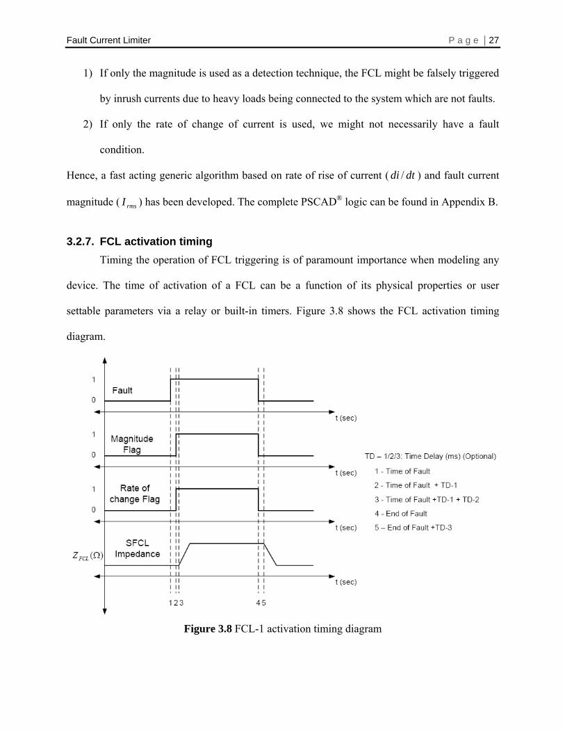
3.2.7. FCL activation timing Timing the operation of FCL triggering is of paramount importance when modeling any
device. The time of activation of a FCL can be a function of its physical properties or user
settable parameters via a relay or built-in timers. Figure 3.8 shows the FCL activation timing
diagram.
Figure 3.8 FCL-1 activation timing diagram
Fault Current Limiter P a g e | 28 From Figure 3.8, a fault is inserted at time 1. Immediately, the magnitude of the line current
increases and the “Magnitude flag” is raised. Also, the “Rate of change flag” is asserted since the
rate at which line current changes is non-zero. After waiting for a few milliseconds (optional),
the impedance of the FCL is ramped up so that the current limiting can proceed. This procedure
is applicable to most of the kinds of FCL.
3.2.8. Implementation methodology In this section, the implementation methodology is presented in order to achieve the
functionality as per flowchart shown in Figure 3.5 for the variable impedance. The following is a
general method of detecting faults and subsequently triggering the SFCL. This methodology is
generic, implying that these concepts can also be extended to other categories and types of FCL.
A. Magnitude, rmsI
There are two ways to monitor a magnitude in PSCAD®:
1) Take the root mean square (RMS) of the line current.
2) Take the phasor value of the current and extract the magnitude.
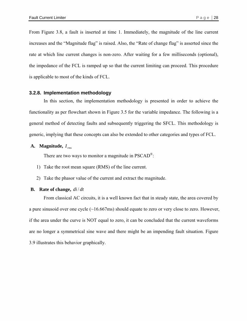
B. Rate of change, dtdi /
From classical AC circuits, it is a well known fact that in steady state, the area covered by
a pure sinusoid over one cycle (~16.667ms) should equate to zero or very close to zero. However,
if the area under the curve is NOT equal to zero, it can be concluded that the current waveforms
are no longer a symmetrical sine wave and there might be an impending fault situation. Figure
3.9 illustrates this behavior graphically.

Fault Current Limiter P a g e | 29
0.285 0.295 0.305 0.315 0.325-7
-6
-5
-4
-3
-2
-1
0
1
2
3
4
5
6
77Line Current waveforms during before and after fault in general
Time (sec)
Line
Cur
rent
(A)
Area C
Area D
Time of Fault
Area BArea A
Area A + Area B = 0 Area C + Area D > 0
Figure 3.9 Line Current waveform before and during a fault
A detection algorithm, using this traditional transient monitor technique has been implemented
by using an integration function to calculate the area under the curve over one cycle.
C. FCL impedance ramping, slope Z
Programming the impedance ramping in the PSCAD® environment is perhaps the most
challenging task. In general the equation for a ramp is given as follows:
Ramp = Starting Point + (Set Point – Starting Point) x Time elapsed
initialZ slopeZRamp Rate: Elapsed time since FCL triggering (3.1)
From 3.1, we see that the impedance of the FCL increases linearly with time. The ramp rate is
user configurable which is a function of the FCL physical properties and design. At this point it
must also be noted that the impedance is clamped to a final value, after which it will not increase
any further.
Fault Current Limiter P a g e | 30
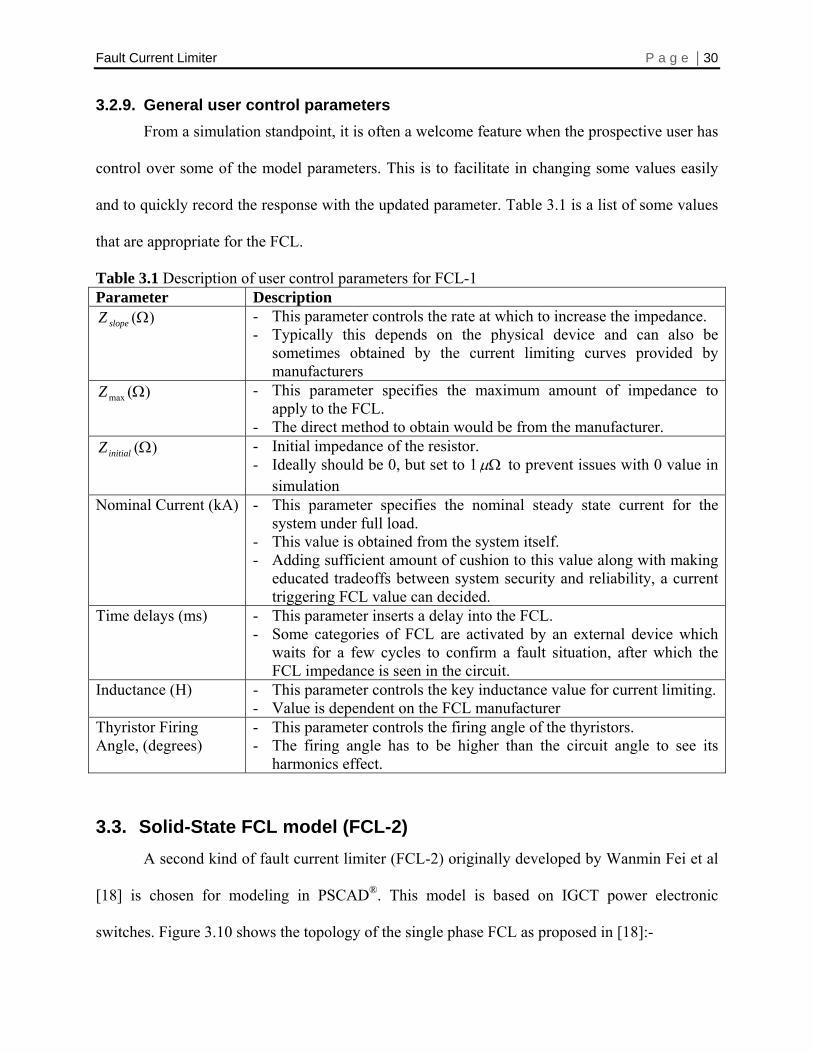
3.2.9. General user control parameters From a simulation standpoint, it is often a welcome feature when the prospective user has
control over some of the model parameters. This is to facilitate in changing some values easily
and to quickly record the response with the updated parameter. Table 3.1 is a list of some values
that are appropriate for the FCL.
Table 3.1 Description of user control parameters for FCL-1 Parameter Description
)(ΩslopeZ - This parameter controls the rate at which to increase the impedance. - Typically this depends on the physical device and can also be
sometimes obtained by the current limiting curves provided by manufacturers
)(max ΩZ - This parameter specifies the maximum amount of impedance to apply to the FCL.
- The direct method to obtain would be from the manufacturer. )(ΩinitialZ - Initial impedance of the resistor.
- Ideally should be 0, but set to 1 Ωμ to prevent issues with 0 value in simulation
Nominal Current (kA) - This parameter specifies the nominal steady state current for the system under full load.
- This value is obtained from the system itself. - Adding sufficient amount of cushion to this value along with making
educated tradeoffs between system security and reliability, a current triggering FCL value can decided.
Time delays (ms) - This parameter inserts a delay into the FCL. - Some categories of FCL are activated by an external device which
waits for a few cycles to confirm a fault situation, after which the FCL impedance is seen in the circuit.
Inductance (H) - This parameter controls the key inductance value for current limiting. - Value is dependent on the FCL manufacturer
Thyristor Firing Angle, (degrees)
- This parameter controls the firing angle of the thyristors. - The firing angle has to be higher than the circuit angle to see its
harmonics effect.
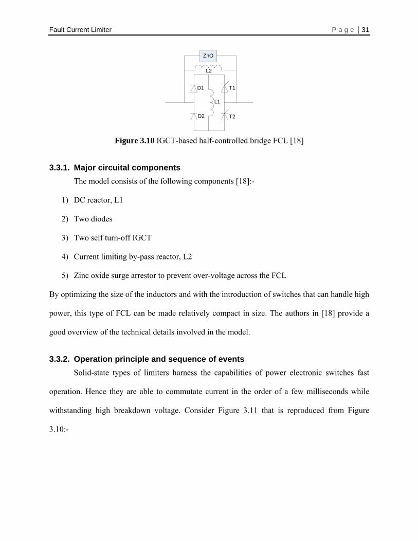
3.3. Solid-State FCL model (FCL-2) A second kind of fault current limiter (FCL-2) originally developed by Wanmin Fei et al
[18] is chosen for modeling in PSCAD®. This model is based on IGCT power electronic
switches. Figure 3.10 shows the topology of the single phase FCL as proposed in [18]:-
Fault Current Limiter P a g e | 31
ZnO
D1
D2 T2
T1
L1
L2
Figure 3.10 IGCT-based half-controlled bridge FCL [18]
3.3.1. Major circuital components The model consists of the following components [18]:-
1) DC reactor, L1
2) Two diodes
3) Two self turn-off IGCT
4) Current limiting by-pass reactor, L2
5) Zinc oxide surge arrestor to prevent over-voltage across the FCL
By optimizing the size of the inductors and with the introduction of switches that can handle high
power, this type of FCL can be made relatively compact in size. The authors in [18] provide a
good overview of the technical details involved in the model.
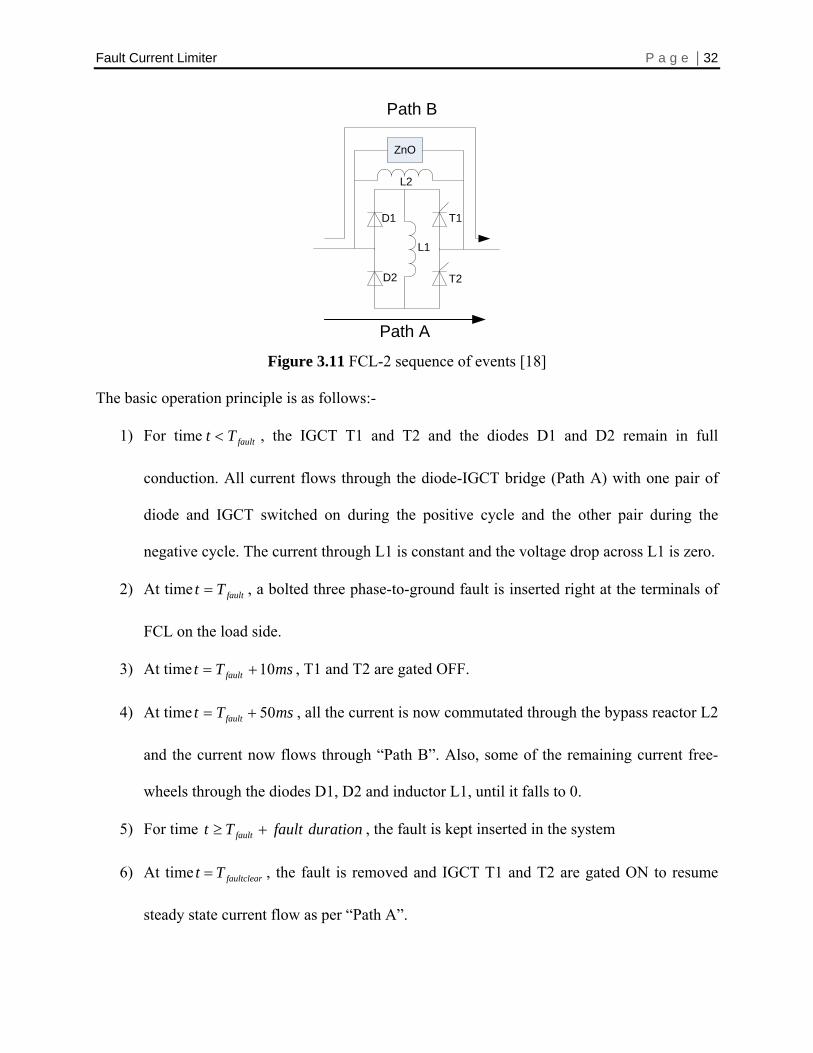
3.3.2. Operation principle and sequence of events Solid-state types of limiters harness the capabilities of power electronic switches fast
operation. Hence they are able to commutate current in the order of a few milliseconds while
withstanding high breakdown voltage. Consider Figure 3.11 that is reproduced from Figure
3.10:-
Fault Current Limiter P a g e | 32
ZnO
D1
D2 T2
T1
L1
L2
Path B
Path A Figure 3.11 FCL-2 sequence of events [18]
The basic operation principle is as follows:-
1) For time faultTt < , the IGCT T1 and T2 and the diodes D1 and D2 remain in full
conduction. All current flows through the diode-IGCT bridge (Path A) with one pair of
diode and IGCT switched on during the positive cycle and the other pair during the
negative cycle. The current through L1 is constant and the voltage drop across L1 is zero.
2) At time faultTt = , a bolted three phase-to-ground fault is inserted right at the terminals of
FCL on the load side.
3) At time ms , T1 and T2 are gated OFF. Tt fault 10+=
4) At time ms , all the current is now commutated through the bypass reactor L2
and the current now flows through “Path B”. Also, some of the remaining current free-
wheels through the diodes D1, D2 and inductor L1, until it falls to 0.
Tt fault 50+=
5) For time duration , the fault is kept inserted in the system faultTt fault +≥
6) At time faultclearTt , the fault is removed and IGCT T1 and T2 are gated ON to resume
steady state current flow as per “Path A”.
=
Fault Current Limiter P a g e | 33
3.3.3. FCL control strategy From the above sequence of events, it is evident that the main control input required for
FCL-2 is the correct time at which to gate the IGCT T1 and T2 OFF so that the current can be
commutated through the bypass inductor L2. To achieve this, it is fundamental to first correctly
detect the fault so that the gating signal can be sent to the two switches. Section 3.2.6, Fault
detection techniques, discussed the methods of detecting a fault and subsequently section 3.2.8
(A, B) discussed the implementation methodology. Building on this rock-solid detection method;
its application is extended to control this FCL and as it is shown in Chapter 4, the FCL performs
satisfactorily. Appendix C shows a detailed implementation of the FCL model in PSCAD®.
3.4. Hybrid FCL model (FCL-3) A third and a final kind of fault current limiter (FCL-3) originally developed by H. Arai
et al [19] is chosen for modeling in PSCAD®. This model is based on the resonance
characteristics exhibited when an inductor and capacitor are in series with each other. Since the
FCL uses solid state as well as superconducting technology, this can be categorized as a hybrid
type of limiter.
3.4.1. Major circuital components The LC resonance based hybrid limiter has just two components, namely an inductor and
a capacitor. However, the interesting aspect of this FCL lies in the fact that the inductor is a
superconducting coil wound with Bi-2223/Ag High Temperature Superconducting tape [19]. It
was mentioned earlier that an inductor wound with HTS wire allows for a very low voltage drop
during steady state while the capacitor acts as a series compensator for the inductive transmission
line. Also, the value of the capacitor and inductor are chosen in such a manner that at nominal
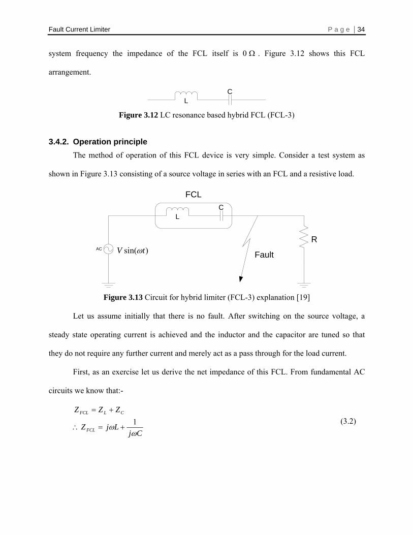
Fault Current Limiter P a g e | 34 system frequency the impedance of the FCL itself is 0 Ω . Figure 3.12 shows this FCL
arrangement.
CL
Figure 3.12 LC resonance based hybrid FCL (FCL-3)
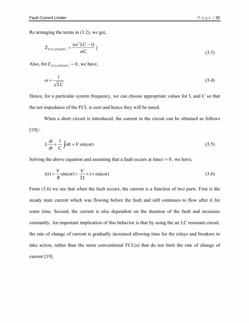
3.4.2. Operation principle The method of operation of this FCL device is very simple. Consider a test system as
shown in Figure 3.13 consisting of a source voltage in series with an FCL and a resistive load.
CL
AC
FCL
R)sin( tV ω Fault
Figure 3.13 Circuit for hybrid limiter (FCL-3) explanation [19]
Let us assume initially that there is no fault. After switching on the source voltage, a
steady state operating current is achieved and the inductor and the capacitor are tuned so that
they do not require any further current and merely act as a pass through for the load current.
First, as an exercise let us derive the net impedance of this FCL. From fundamental AC
circuits we know that:-
CjLjZ
ZZZ
FCL
CLFCL
ωω 1
+=∴
+= (3.2)
Fault Current Limiter P a g e | 35 Re arranging the terms in (3.2), we get,
jC
LCZ STEADYFCL ωω )1( 2
)(−
= (3.3)
Also, for , we have, 0)( =STEADYFCLZ
LC1
=ω (3.4)
Hence, for a particular system frequency, we can choose appropriate values for L and C so that
the net impedance of the FCL is zero and hence they will be tuned.
When a short circuit is introduced, the current in the circuit can be obtained as follows
[19]:-
)sin(1 tVidtCdt
diL ω=+ ∫ (3.5)
Solving the above equation and assuming that a fault occurs at time 0=t , we have;
)sin(2
)sin()( ttL
VtRVti ωω ××+= (3.6)
From (3.6) we see that when the fault occurs, the current is a function of two parts. First is the
steady state current which was flowing before the fault and still continues to flow after it for
some time. Second, the current is also dependent on the duration of the fault and increases
constantly. An important implication of this behavior is that by using the an LC resonant circuit,
the rate of change of current is gradually increased allowing time for the relays and breakers to
take action, rather than the more conventional FCL(s) that do not limit the rate of change of
current [19].
Fault Current Limiter P a g e | 36
3.4.3. Sequence of events The sequence of events for FCL-3 is as follows:-
1) For time faultTt < , the source voltage supplies regular current to the load through FCL-3.
Since L and C are tuned to the source voltage frequency, there is negligible impedance
from the FCL itself
2) At time faultTt = , a bolted three phase-to-ground fault is inserted right at the terminals of
FCL-3 on the load side.
3) At time faultTt > , the FCL is de-tuned from resonance and the current is limited by the
inductor
4) For time duration , the fault is kept inserted in the system faultTt fault +≥
5) At time faultclearTt , the fault is removed and the FCL goes back to the resonance state. =
Chapter 4 will show in detail the results obtained by simulating this FCL.
Fault Current Limiter P a g e | 37
Chapter 4. SIMULATION RESULTS This chapter presents the results obtained from the FCL modeling efforts in chapter 3. A
brief overview about the test bed and case studies are described.
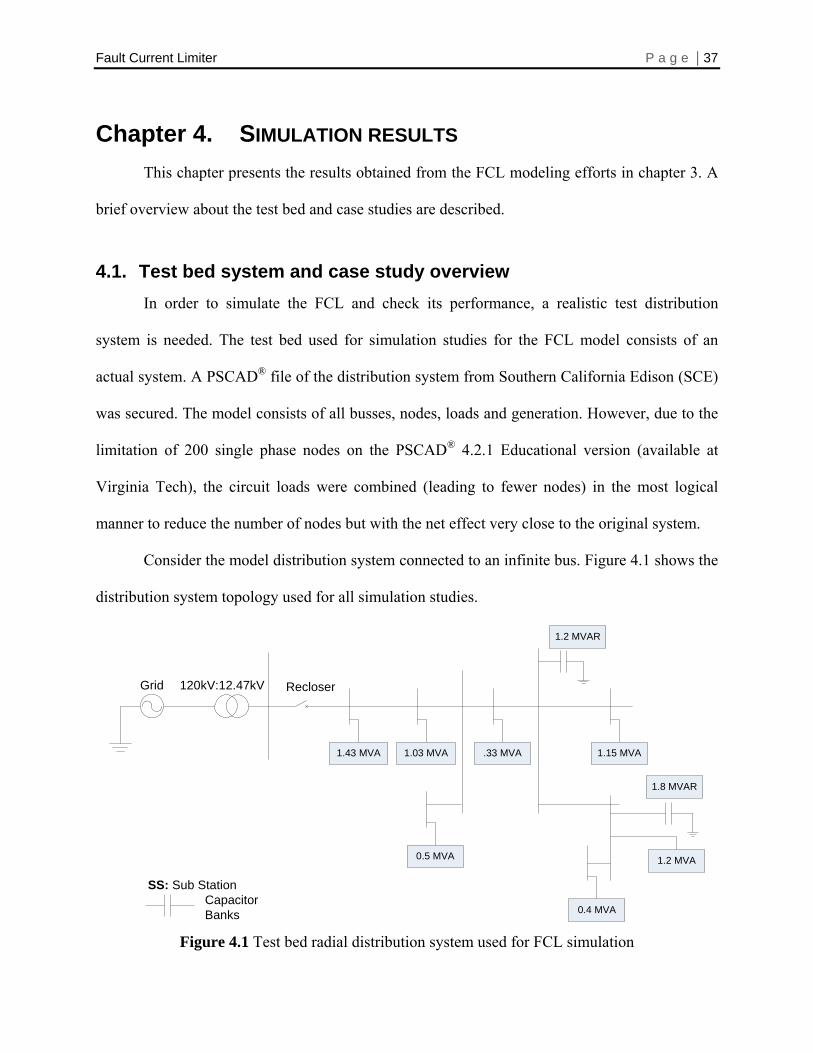
4.1. Test bed system and case study overview In order to simulate the FCL and check its performance, a realistic test distribution
system is needed. The test bed used for simulation studies for the FCL model consists of an
actual system. A PSCAD® file of the distribution system from Southern California Edison (SCE)
was secured. The model consists of all busses, nodes, loads and generation. However, due to the
limitation of 200 single phase nodes on the PSCAD® 4.2.1 Educational version (available at
Virginia Tech), the circuit loads were combined (leading to fewer nodes) in the most logical
manner to reduce the number of nodes but with the net effect very close to the original system.
Consider the model distribution system connected to an infinite bus. Figure 4.1 shows the
distribution system topology used for all simulation studies.
Grid 120kV:12.47kV Recloser
1.43 MVA .33 MVA 1.15 MVA
1.2 MVA
0.4 MVA
0.5 MVA
1.2 MVAR
1.8 MVAR
Capacitor Banks
SS: Sub Station
1.03 MVA
Figure 4.1 Test bed radial distribution system used for FCL simulation
Fault Current Limiter P a g e | 38 Some of the key parameters of this system at an aggregate level are summarized in Table 4.1
Table 4.1 Summary of test system steady-state parameters Parameter Value Operating Voltage LLkV5.12≈ Nominal Line Current rmsA260≈ Net Load 5.82 MVA (incl. transmission losses, 0.74MW) System Frequency 60 Hz Number of Busses 45 (not all shown) Substation Transformer 120 kV / 12.5 kV Line Types Underground and Overhead
A total of five case studies involving the three modeled FCL(s) are conducted. Out of the
five, the first three involve superconducting FCL (FCL-1). The three FCL-1 cases are as follows:
1) The distribution system with and without an FCL-1 to check for current and voltage
waveforms, effect on real and reactive power and time required by the FCL to reduce the
fault current to a pre-determined level.
2) A comparative study between the developed HTS FCL-1 model and FCL commissioned
by Z-energy. Emphasis has been given on achieving a very close behavior by FCL-1 to
the one by Z-Energy.
3) The overall impact assessment of the FCL-1 device in the operation of sectionalizers and
relay co-ordination.
The last two case studies investigate the operation and behavior of the solid state FCL (FCL-2)
and the hybrid limiter (FCL-3). Along with these cases, Table 4.2 summarizes the simulation
settings that were used in PSCAD®:-
Table 4.2 Simulation Parameter settings Parameter Value Total simulation time 1 second Time of fault insertion 0.3 seconds Duration of fault 0.5 seconds (30 cycles) Type of fault ABC G Scan time 0.1 ms

Fault Current Limiter P a g e | 39 A bolted three phase-to-ground fault is used in all simulations as this will produce the highest
amount of fault current. This is the worst case scenario for the given distribution system. This
also helps in sizing the FCL parameters accordingly, since the device will be certain to work for
any other type of fault (like phase-to-ground and phase-to-phase fault) with a lesser fault current
value than a three phase to ground fault. Also, dedicated logic was developed in order to
facilitate the insertion of the fault at the zero crossing (from negative to positive) of the voltage.
This ensures that the current will be at its peak and worst the case scenario can be analyzed.
Before getting into the details of the results, let us establish some of the threshold
magnitudes of fault currents that are observed in this particular distribution system. Table 4.3
shows the peak and the steady state faulted current values for faults placed at increasing
distances from the main substation recloser.
Table 4.3 Line current values for fault at different distances from recloser Fault Distance (meters) Line Current ( ) rmskA Peak current at time of fault Steady state while faulted
0 30.4 19.8 3200 12.9 10.8 5900 8.60 7.50 7500 7.02 6.25
As expected, that as the distance of the fault is increased from the re-closer; the magnitude of the
fault current level reduces. The objective of the FCL is to mitigate the fault current in the event
of a fault being inserted right at the terminals on the load side and generation connected at the
source side of the FCL (Note: the distribution system is radial in nature). This will result in the
maximum amount of fault current levels. From Table 4.3, it is clear that the FCL must be able to
withstand a steady state faulted current level of at least 19.8 kA and a surge current of 30.4 kA
for the first few cycles. Building on this basis, the results of the study are presented below.
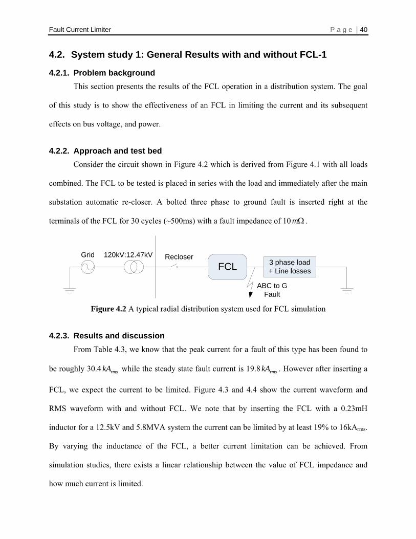
Fault Current Limiter P a g e | 40
4.2. System study 1: General Results with and without FCL-1
4.2.1. Problem background This section presents the results of the FCL operation in a distribution system. The goal
of this study is to show the effectiveness of an FCL in limiting the current and its subsequent
effects on bus voltage, and power.
4.2.2. Approach and test bed Consider the circuit shown in Figure 4.2 which is derived from Figure 4.1 with all loads
combined. The FCL to be tested is placed in series with the load and immediately after the main
substation automatic re-closer. A bolted three phase to ground fault is inserted right at the
terminals of the FCL for 30 cycles (~500ms) with a fault impedance of 10 . Ωm
Grid 120kV:12.47kV RecloserFCL 3 phase load
+ Line losses
ABC to GFault
Figure 4.2 A typical radial distribution system used for FCL simulation
4.2.3. Results and discussion From Table 4.3, we know that the peak current for a fault of this type has been found to
be roughly 30.4 while the steady state fault current is 19.8 . However after inserting a
FCL, we expect the current to be limited. Figure 4.3 and 4.4 show the current waveform and
RMS waveform with and without FCL. We note that by inserting the FCL with a 0.23mH
inductor for a 12.5kV and 5.8MVA system the current can be limited by at least 19% to 16kArms.
By varying the inductance of the FCL, a better current limitation can be achieved. From
simulation studies, there exists a linear relationship between the value of FCL impedance and
how much current is limited.
rmskA rmskA
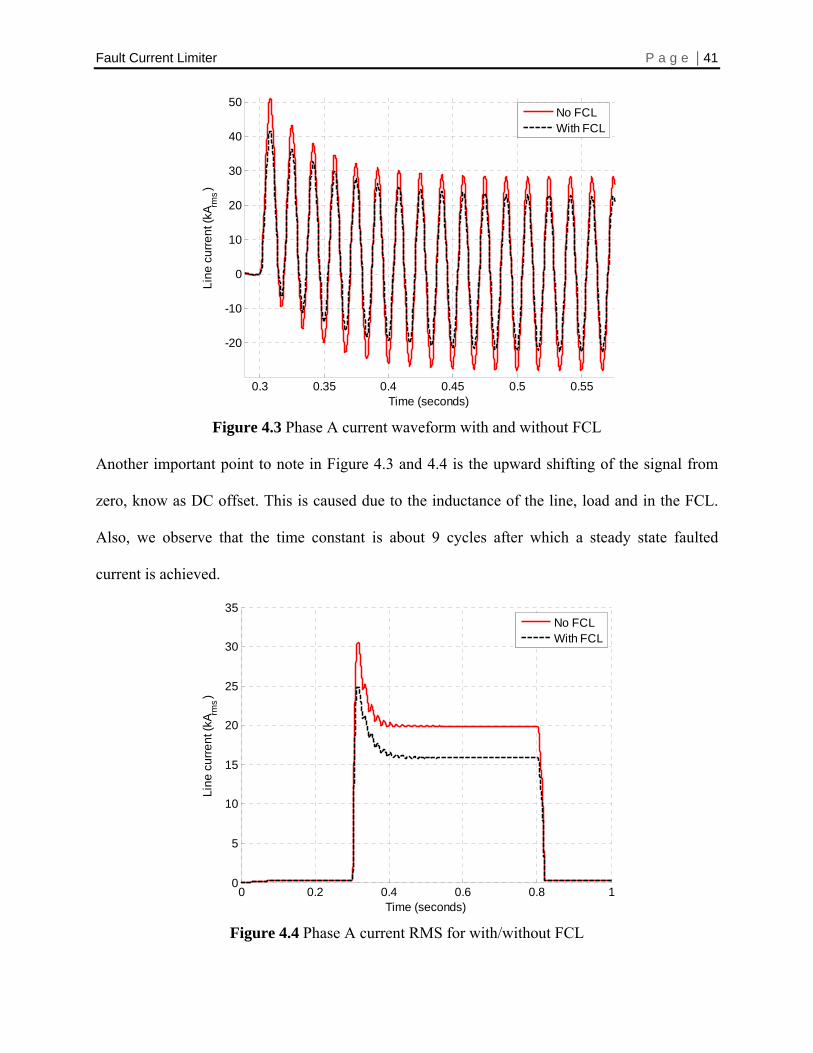
Fault Current Limiter P a g e | 41
0.3 0.35 0.4 0.45 0.5 0.55
-20
-10
0
10
20
30
40
50
Time (seconds)
Line
cur
rent
(kA rm
s)
No FCLWith FCL
Figure 4.3 Phase A current waveform with and without FCL
Another important point to note in Figure 4.3 and 4.4 is the upward shifting of the signal from
zero, know as DC offset. This is caused due to the inductance of the line, load and in the FCL.
Also, we observe that the time constant is about 9 cycles after which a steady state faulted
current is achieved.
0 0.2 0.4 0.6 0.8 10
5
10
15
20
25
30
35
Time (seconds)
Line
cur
rent
(kA rm
s)
No FCLWith FCL
Figure 4.4 Phase A current RMS for with/without FCL
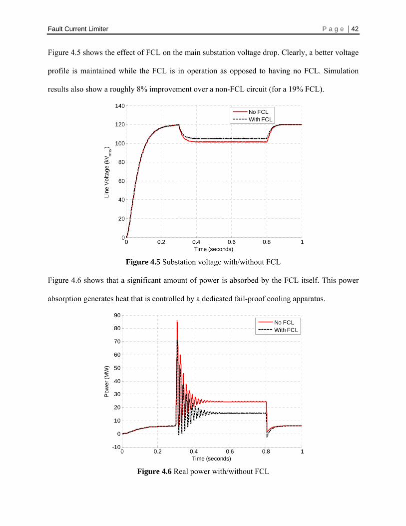
Fault Current Limiter P a g e | 42 Figure 4.5 shows the effect of FCL on the main substation voltage drop. Clearly, a better voltage
profile is maintained while the FCL is in operation as opposed to having no FCL. Simulation
results also show a roughly 8% improvement over a non-FCL circuit (for a 19% FCL).
0 0.2 0.4 0.6 0.8 10
20
40
60
80
100
120
140
Time (seconds)
Line
Vol
tage
(kV rm
s)
No FCLWith FCL
Figure 4.5 Substation voltage with/without FCL
Figure 4.6 shows that a significant amount of power is absorbed by the FCL itself. This power
absorption generates heat that is controlled by a dedicated fail-proof cooling apparatus.
0 0.2 0.4 0.6 0.8 1-10
0
10
20
30
40
50
60
70
80
90
Time (seconds)
Pow
er (M
W)
No FCLWith FCL
Figure 4.6 Real power with/without FCL
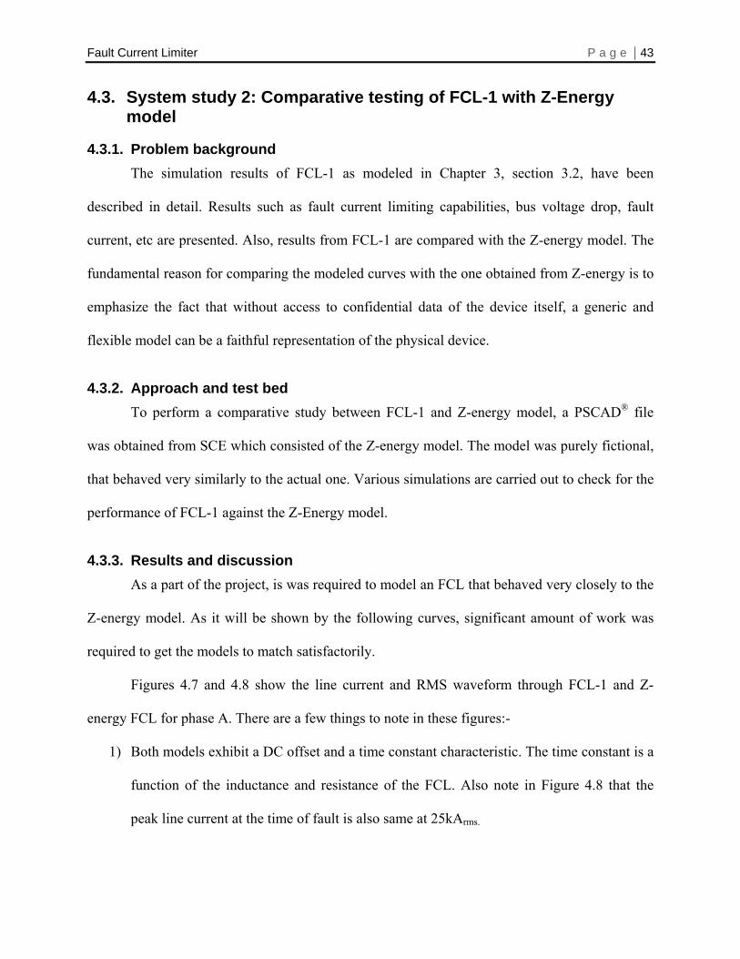
Fault Current Limiter P a g e | 43
4.3. System study 2: Comparative testing of FCL-1 with Z-Energy model
4.3.1. Problem background The simulation results of FCL-1 as modeled in Chapter 3, section 3.2, have been
described in detail. Results such as fault current limiting capabilities, bus voltage drop, fault
current, etc are presented. Also, results from FCL-1 are compared with the Z-energy model. The
fundamental reason for comparing the modeled curves with the one obtained from Z-energy is to
emphasize the fact that without access to confidential data of the device itself, a generic and
flexible model can be a faithful representation of the physical device.
4.3.2. Approach and test bed To perform a comparative study between FCL-1 and Z-energy model, a PSCAD® file
was obtained from SCE which consisted of the Z-energy model. The model was purely fictional,
that behaved very similarly to the actual one. Various simulations are carried out to check for the
performance of FCL-1 against the Z-Energy model.
4.3.3. Results and discussion As a part of the project, is was required to model an FCL that behaved very closely to the
Z-energy model. As it will be shown by the following curves, significant amount of work was
required to get the models to match satisfactorily.
Figures 4.7 and 4.8 show the line current and RMS waveform through FCL-1 and Z-
energy FCL for phase A. There are a few things to note in these figures:-
1) Both models exhibit a DC offset and a time constant characteristic. The time constant is a
function of the inductance and resistance of the FCL. Also note in Figure 4.8 that the
peak line current at the time of fault is also same at 25kArms.
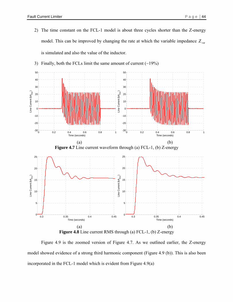
Fault Current Limiter P a g e | 44
2) The time constant on the FCL-1 model is about three cycles shorter than the Z-energy
model. This can be improved by changing the rate at which the variable impedance varZ
is simulated and also the value of the inductor.
3) Finally, both the FCLs limit the same amount of current (~19%)
0 0.2 0.4 0.6 0.8 1-30
-20
-10
0
10
20
30
40
50
Time (seconds)
Line
Cur
rent
(kA rm
s)
0 0.2 0.4 0.6 0.8 1-30
-20
-10
0
10
20
30
40
50
Time (seconds)
Line
Cur
rent
(kA rm
s)
(a) (b)
Figure 4.7 Line current waveform through (a) FCL-1, (b) Z-energy
0.3 0.35 0.4 0.450
5
10
15
20
25
Time (seconds)
Line
Cur
rent
(kA rm
s)
0.3 0.35 0.4 0.450
5
10
15
20
25
Time (seconds)
Line
Cur
rent
(kA rm
s)
(a) (b)
Figure 4.8 Line current RMS through (a) FCL-1, (b) Z-energy
Figure 4.9 is the zoomed version of Figure 4.7. As we outlined earlier, the Z-energy
model showed evidence of a strong third harmonic component (Figure 4.9 (b)). This is also been
incorporated in the FCL-1 model which is evident from Figure 4.9(a)
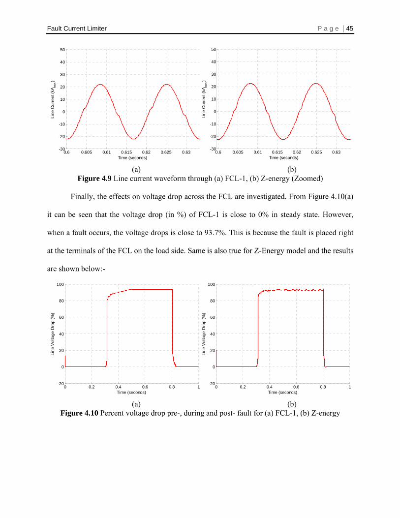
Fault Current Limiter P a g e | 45
0.6 0.605 0.61 0.615 0.62 0.625 0.63-30
-20
-10
0
10
20
30
40
50
Time (seconds)
Line
Cur
rent
(kA rm
s)
0.6 0.605 0.61 0.615 0.62 0.625 0.63-30
-20
-10
0
10
20
30
40
50
Time (seconds)
Line
Cur
rent
(kA rm
s)
(a) (b)
Figure 4.9 Line current waveform through (a) FCL-1, (b) Z-energy (Zoomed)
Finally, the effects on voltage drop across the FCL are investigated. From Figure 4.10(a)
it can be seen that the voltage drop (in %) of FCL-1 is close to 0% in steady state. However,
when a fault occurs, the voltage drops is close to 93.7%. This is because the fault is placed right
at the terminals of the FCL on the load side. Same is also true for Z-Energy model and the results
are shown below:-
0 0.2 0.4 0.6 0.8 1-20
0
20
40
60
80
100
Time (seconds)
Line
Vol
tage
Dro
p (%
)
0 0.2 0.4 0.6 0.8 1-20
0
20
40
60
80
100
Time (seconds)
Line
Vol
tage
Dro
p (%
)
(a) (b)
Figure 4.10 Percent voltage drop pre-, during and post- fault for (a) FCL-1, (b) Z-energy
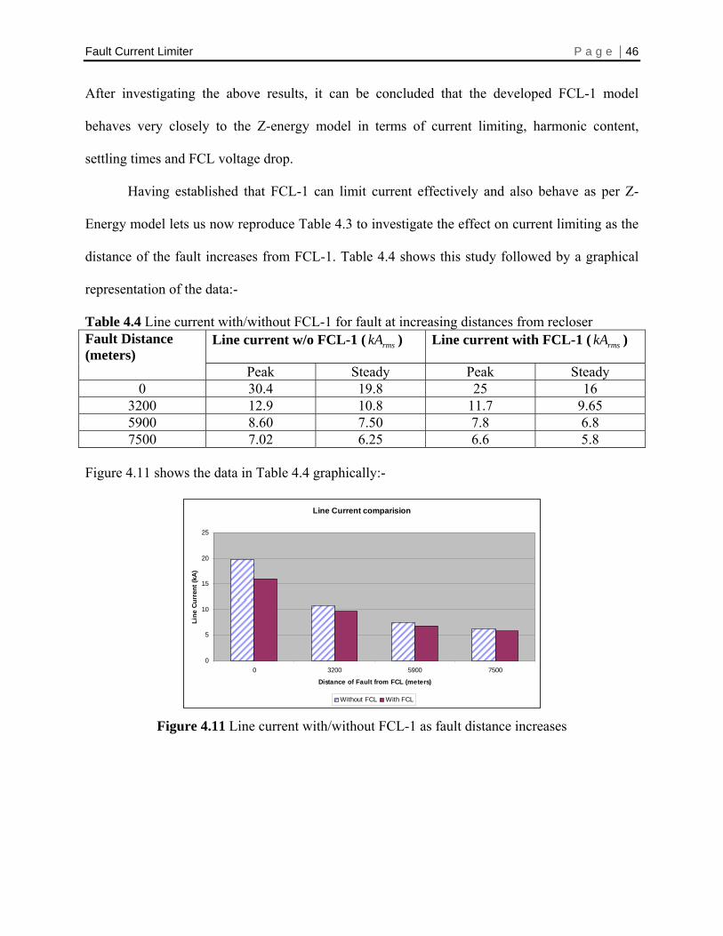
Fault Current Limiter P a g e | 46 After investigating the above results, it can be concluded that the developed FCL-1 model
behaves very closely to the Z-energy model in terms of current limiting, harmonic content,
settling times and FCL voltage drop.
Having established that FCL-1 can limit current effectively and also behave as per Z-
Energy model lets us now reproduce Table 4.3 to investigate the effect on current limiting as the
distance of the fault increases from FCL-1. Table 4.4 shows this study followed by a graphical
representation of the data:-
Table 4.4 Line current with/without FCL-1 for fault at increasing distances from recloser Fault Distance (meters)
Line current w/o FCL-1 ( ) rmskA Line current with FCL-1 ( ) rmskA
Peak Steady Peak Steady 0 30.4 19.8 25 16
3200 12.9 10.8 11.7 9.65 5900 8.60 7.50 7.8 6.8 7500 7.02 6.25 6.6 5.8
Figure 4.11 shows the data in Table 4.4 graphically:-
Line Current comparision
0
5
10
15
20
25
0 3200 5900 7500
Distance of Fault from FCL (meters)
Line
Cur
rent
(kA)
Without FCL With FCL Figure 4.11 Line current with/without FCL-1 as fault distance increases
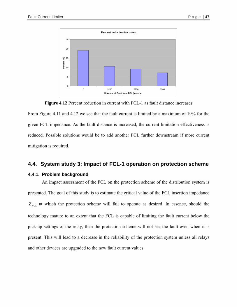
Fault Current Limiter P a g e | 47
Percent reduction in current
0
5
10
15
20
25
0 3200 5900 7500
Distance of Fault from FCL (meters)
Perc
ent (
%)
Figure 4.12 Percent reduction in current with FCL-1 as fault distance increases
From Figure 4.11 and 4.12 we see that the fault current is limited by a maximum of 19% for the
given FCL impedance. As the fault distance is increased, the current limitation effectiveness is
reduced. Possible solutions would be to add another FCL further downstream if more current
mitigation is required.
4.4. System study 3: Impact of FCL-1 operation on protection scheme
4.4.1. Problem background An impact assessment of the FCL on the protection scheme of the distribution system is
presented. The goal of this study is to estimate the critical value of the FCL insertion impedance
at which the protection scheme will fail to operate as desired. In essence, should the
technology mature to an extent that the FCL is capable of limiting the fault current below the
pick-up settings of the relay, then the protection scheme will not see the fault even when it is
present. This will lead to a decrease in the reliability of the protection system unless all relays
and other devices are upgraded to the new fault current values.
FCLZ
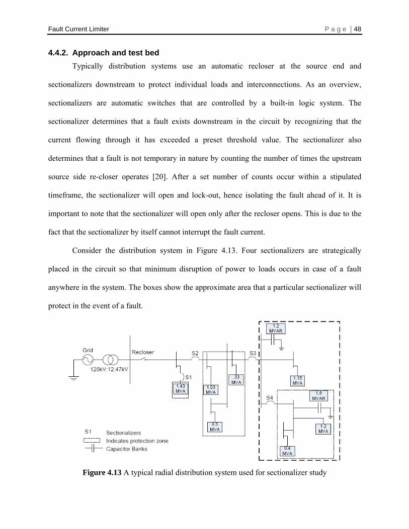
Fault Current Limiter P a g e | 48
4.4.2. Approach and test bed Typically distribution systems use an automatic recloser at the source end and
sectionalizers downstream to protect individual loads and interconnections. As an overview,
sectionalizers are automatic switches that are controlled by a built-in logic system. The
sectionalizer determines that a fault exists downstream in the circuit by recognizing that the
current flowing through it has exceeded a preset threshold value. The sectionalizer also
determines that a fault is not temporary in nature by counting the number of times the upstream
source side re-closer operates [20]. After a set number of counts occur within a stipulated
timeframe, the sectionalizer will open and lock-out, hence isolating the fault ahead of it. It is
important to note that the sectionalizer will open only after the recloser opens. This is due to the
fact that the sectionalizer by itself cannot interrupt the fault current.
Consider the distribution system in Figure 4.13. Four sectionalizers are strategically
placed in the circuit so that minimum disruption of power to loads occurs in case of a fault
anywhere in the system. The boxes show the approximate area that a particular sectionalizer will
protect in the event of a fault.
Figure 4.13 A typical radial distribution system used for sectionalizer study
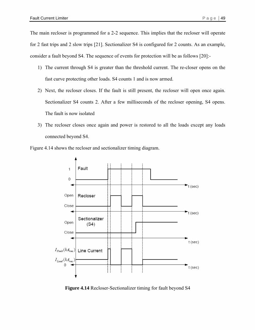
Fault Current Limiter P a g e | 49 The main recloser is programmed for a 2-2 sequence. This implies that the recloser will operate
for 2 fast trips and 2 slow trips [21]. Sectionalizer S4 is configured for 2 counts. As an example,
consider a fault beyond S4. The sequence of events for protection will be as follows [20]:-
1) The current through S4 is greater than the threshold current. The re-closer opens on the
fast curve protecting other loads. S4 counts 1 and is now armed.
2) Next, the recloser closes. If the fault is still present, the recloser will open once again.
Sectionalizer S4 counts 2. After a few milliseconds of the recloser opening, S4 opens.
The fault is now isolated
3) The recloser closes once again and power is restored to all the loads except any loads
connected beyond S4.
Figure 4.14 shows the recloser and sectionalizer timing diagram.
Figure 4.14 Recloser-Sectionalizer timing for fault beyond S4
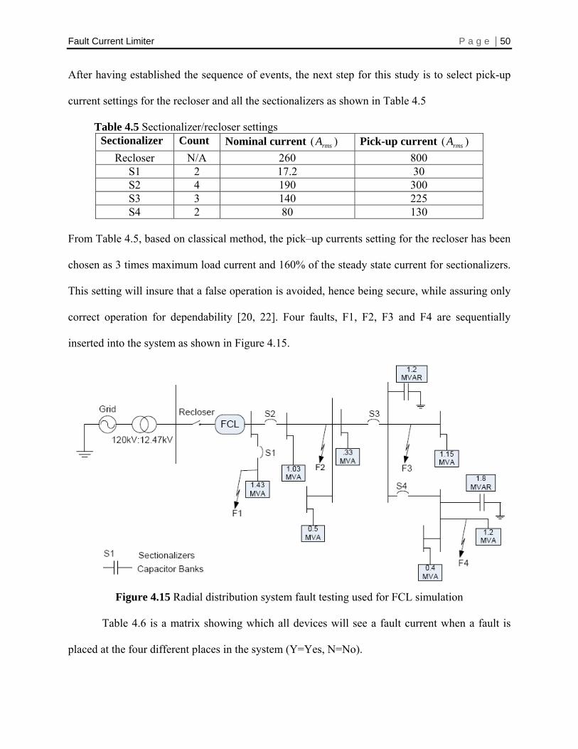
Fault Current Limiter P a g e | 50 After having established the sequence of events, the next step for this study is to select pick-up
current settings for the recloser and all the sectionalizers as shown in Table 4.5
Table 4.5 Sectionalizer/recloser settings Sectionalizer Count Nominal current )( rmsA Pick-up current )( rmsA
Recloser N/A 260 800 S1 2 17.2 30 S2 4 190 300 S3 3 140 225 S4 2 80 130
From Table 4.5, based on classical method, the pick–up currents setting for the recloser has been
chosen as 3 times maximum load current and 160% of the steady state current for sectionalizers.
This setting will insure that a false operation is avoided, hence being secure, while assuring only
correct operation for dependability [20, 22]. Four faults, F1, F2, F3 and F4 are sequentially
inserted into the system as shown in Figure 4.15.
Figure 4.15 Radial distribution system fault testing used for FCL simulation
Table 4.6 is a matrix showing which all devices will see a fault current when a fault is
placed at the four different places in the system (Y=Yes, N=No).
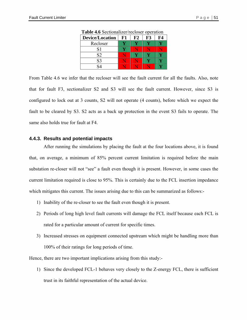
Fault Current Limiter P a g e | 51
Table 4.6 Sectionalizer/recloser operation Device/Location F1 F2 F3 F4
Recloser Y Y Y Y S1 Y N N N S2 N Y Y Y S3 N N Y Y S4 N N N Y
From Table 4.6 we infer that the recloser will see the fault current for all the faults. Also, note
that for fault F3, sectionalizer S2 and S3 will see the fault current. However, since S3 is
configured to lock out at 3 counts, S2 will not operate (4 counts), before which we expect the
fault to be cleared by S3. S2 acts as a back up protection in the event S3 fails to operate. The
same also holds true for fault at F4.
4.4.3. Results and potential impacts After running the simulations by placing the fault at the four locations above, it is found
that, on average, a minimum of 85% percent current limitation is required before the main
substation re-closer will not “see” a fault even though it is present. However, in some cases the
current limitation required is close to 95%. This is certainly due to the FCL insertion impedance
which mitigates this current. The issues arising due to this can be summarized as follows:-
1) Inability of the re-closer to see the fault even though it is present.
2) Periods of long high level fault currents will damage the FCL itself because each FCL is
rated for a particular amount of current for specific times.
3) Increased stresses on equipment connected upstream which might be handling more than
100% of their ratings for long periods of time.
Hence, there are two important implications arising from this study:-
1) Since the developed FCL-1 behaves very closely to the Z-energy FCL, there is sufficient
trust in its faithful representation of the actual device.
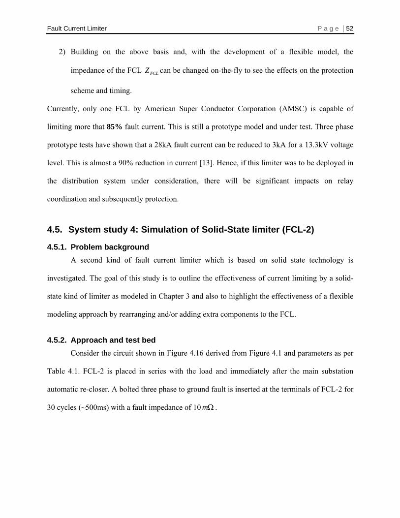
Fault Current Limiter P a g e | 52
2) Building on the above basis and, with the development of a flexible model, the
impedance of the FCL FCLZ can be changed on-the-fly to see the effects on the protection
scheme and timing.
Currently, only one FCL by American Super Conductor Corporation (AMSC) is capable of
limiting more that 85% fault current. This is still a prototype model and under test. Three phase
prototype tests have shown that a 28kA fault current can be reduced to 3kA for a 13.3kV voltage
level. This is almost a 90% reduction in current [13]. Hence, if this limiter was to be deployed in
the distribution system under consideration, there will be significant impacts on relay
coordination and subsequently protection.
4.5. System study 4: Simulation of Solid-State limiter (FCL-2)
4.5.1. Problem background A second kind of fault current limiter which is based on solid state technology is
investigated. The goal of this study is to outline the effectiveness of current limiting by a solid-
state kind of limiter as modeled in Chapter 3 and also to highlight the effectiveness of a flexible
modeling approach by rearranging and/or adding extra components to the FCL.
4.5.2. Approach and test bed Consider the circuit shown in Figure 4.16 derived from Figure 4.1 and parameters as per
Table 4.1. FCL-2 is placed in series with the load and immediately after the main substation
automatic re-closer. A bolted three phase to ground fault is inserted at the terminals of FCL-2 for
30 cycles (~500ms) with a fault impedance of 10 Ωm .
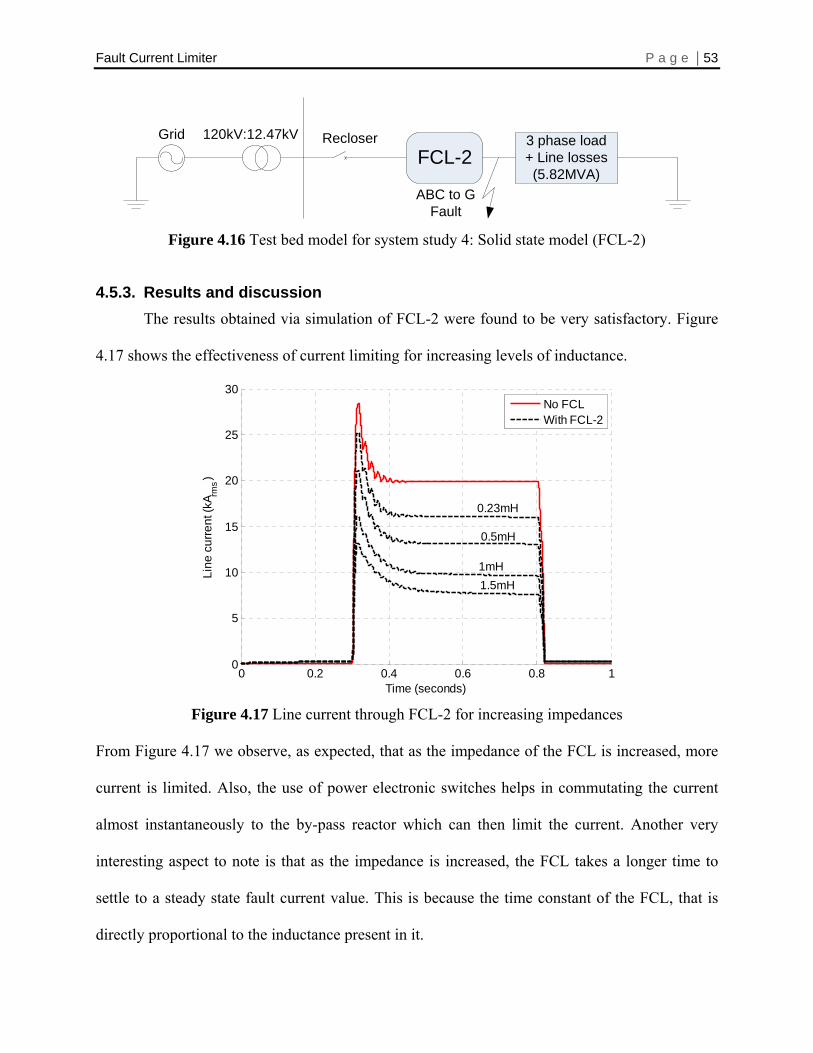
Fault Current Limiter P a g e | 53
Grid 120kV:12.47kV RecloserFCL-2
3 phase load + Line losses(5.82MVA)
ABC to GFault
Figure 4.16 Test bed model for system study 4: Solid state model (FCL-2)
4.5.3. Results and discussion The results obtained via simulation of FCL-2 were found to be very satisfactory. Figure
4.17 shows the effectiveness of current limiting for increasing levels of inductance.
0 0.2 0.4 0.6 0.8 10
5
10
15
20
25
30
Time (seconds)
Line
cur
rent
(kA rm
s)
No FCLWith FCL-2
0.23mH
0.5mH
1mH1.5mH
Figure 4.17 Line current through FCL-2 for increasing impedances
From Figure 4.17 we observe, as expected, that as the impedance of the FCL is increased, more
current is limited. Also, the use of power electronic switches helps in commutating the current
almost instantaneously to the by-pass reactor which can then limit the current. Another very
interesting aspect to note is that as the impedance is increased, the FCL takes a longer time to
settle to a steady state fault current value. This is because the time constant of the FCL, that is
directly proportional to the inductance present in it.
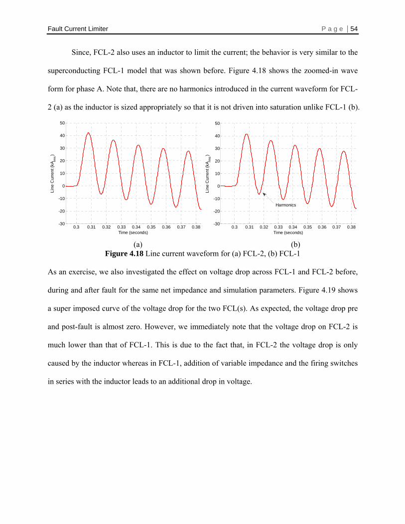
Fault Current Limiter P a g e | 54
Since, FCL-2 also uses an inductor to limit the current; the behavior is very similar to the
superconducting FCL-1 model that was shown before. Figure 4.18 shows the zoomed-in wave
form for phase A. Note that, there are no harmonics introduced in the current waveform for FCL-
2 (a) as the inductor is sized appropriately so that it is not driven into saturation unlike FCL-1 (b).
0.3 0.31 0.32 0.33 0.34 0.35 0.36 0.37 0.38-30
-20
-10
0
10
20
30
40
50
Time (seconds)
Line
Cur
rent
(kA rm
s)
0.3 0.31 0.32 0.33 0.34 0.35 0.36 0.37 0.38
-30
-20
-10
0
10
20
30
40
50
Time (seconds)
Line
Cur
rent
(kA rm
s)Harmonics
(a) (b)
Figure 4.18 Line current waveform for (a) FCL-2, (b) FCL-1 As an exercise, we also investigated the effect on voltage drop across FCL-1 and FCL-2 before,
during and after fault for the same net impedance and simulation parameters. Figure 4.19 shows
a super imposed curve of the voltage drop for the two FCL(s). As expected, the voltage drop pre
and post-fault is almost zero. However, we immediately note that the voltage drop on FCL-2 is
much lower than that of FCL-1. This is due to the fact that, in FCL-2 the voltage drop is only
caused by the inductor whereas in FCL-1, addition of variable impedance and the firing switches
in series with the inductor leads to an additional drop in voltage.
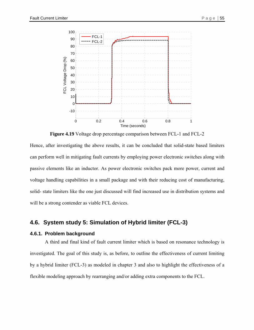
Fault Current Limiter P a g e | 55
0 0.2 0.4 0.6 0.8 1
-10
0
10
20
30
40
50
60
70
80
90
100
Time (seconds)
FCL
Vol
tage
Dro
p (%
)
FCL-1FCL-2
Figure 4.19 Voltage drop percentage comparison between FCL-1 and FCL-2
Hence, after investigating the above results, it can be concluded that solid-state based limiters
can perform well in mitigating fault currents by employing power electronic switches along with
passive elements like an inductor. As power electronic switches pack more power, current and
voltage handling capabilities in a small package and with their reducing cost of manufacturing,
solid- state limiters like the one just discussed will find increased use in distribution systems and
will be a strong contender as viable FCL devices.
4.6. System study 5: Simulation of Hybrid limiter (FCL-3)
4.6.1. Problem background A third and final kind of fault current limiter which is based on resonance technology is
investigated. The goal of this study is, as before, to outline the effectiveness of current limiting
by a hybrid limiter (FCL-3) as modeled in chapter 3 and also to highlight the effectiveness of a
flexible modeling approach by rearranging and/or adding extra components to the FCL.
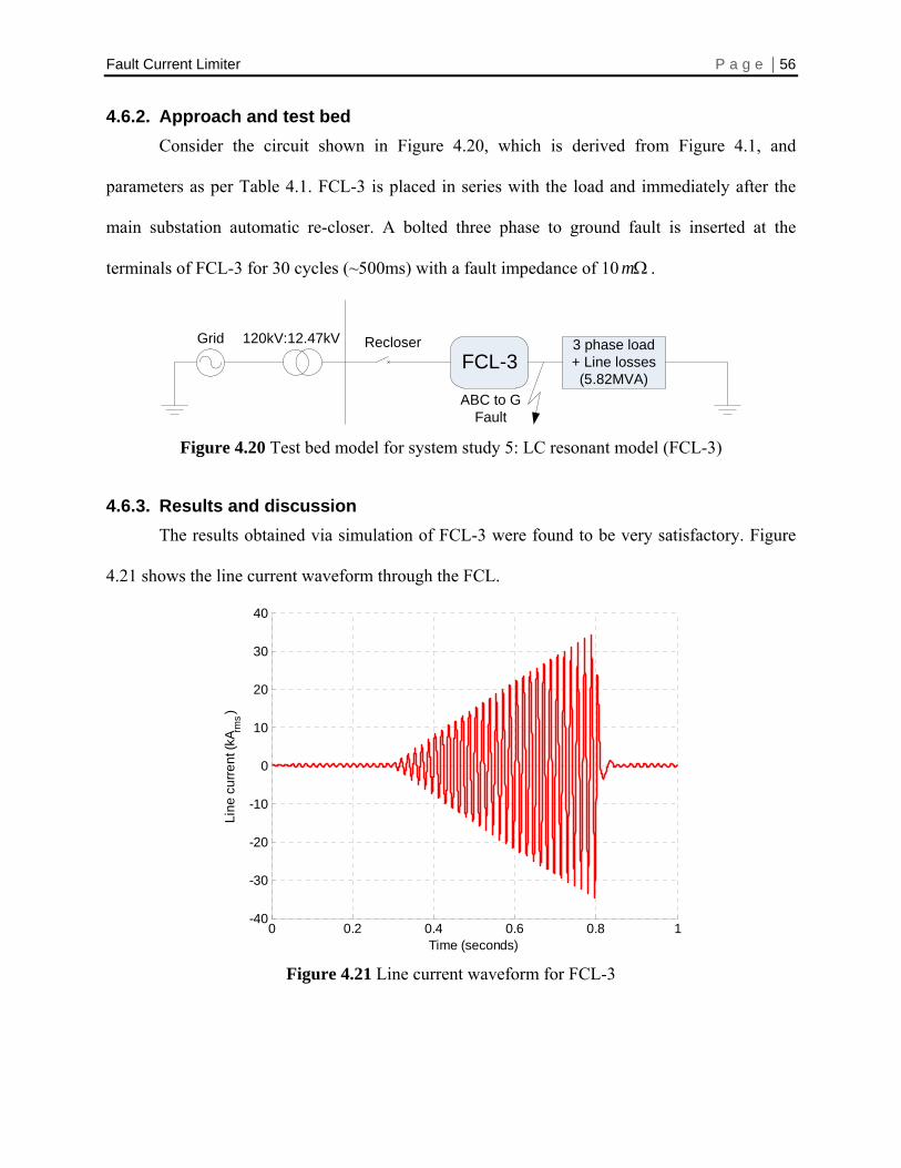
Fault Current Limiter P a g e | 56
4.6.2. Approach and test bed Consider the circuit shown in Figure 4.20, which is derived from Figure 4.1, and
parameters as per Table 4.1. FCL-3 is placed in series with the load and immediately after the
main substation automatic re-closer. A bolted three phase to ground fault is inserted at the
terminals of FCL-3 for 30 cycles (~500ms) with a fault impedance of 10 . Ωm
Grid 120kV:12.47kV RecloserFCL-3
3 phase load + Line losses(5.82MVA)
ABC to GFault
Figure 4.20 Test bed model for system study 5: LC resonant model (FCL-3)
4.6.3. Results and discussion The results obtained via simulation of FCL-3 were found to be very satisfactory. Figure
4.21 shows the line current waveform through the FCL.
0 0.2 0.4 0.6 0.8 1-40
-30
-20
-10
0
10
20
30
40
Time (seconds)
Line
cur
rent
(kA rm
s)
Figure 4.21 Line current waveform for FCL-3
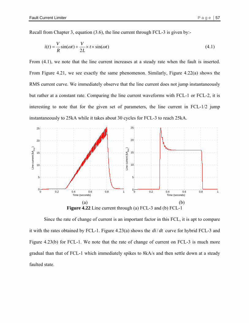
Fault Current Limiter P a g e | 57 Recall from Chapter 3, equation (3.6), the line current through FCL-3 is given by:-
)sin(2
)sin()( ttL
VtRVti ωω ××+= (4.1)
From (4.1), we note that the line current increases at a steady rate when the fault is inserted.
From Figure 4.21, we see exactly the same phenomenon. Similarly, Figure 4.22(a) shows the
RMS current curve. We immediately observe that the line current does not jump instantaneously
but rather at a constant rate. Comparing the line current waveforms with FCL-1 or FCL-2, it is
interesting to note that for the given set of parameters, the line current in FCL-1/2 jump
instantaneously to 25kA while it takes about 30 cycles for FCL-3 to reach 25kA.
0 0.2 0.4 0.6 0.8 10
5
10
15
20
25
Time (seconds)
Line
cur
rent
(kA rm
s)
0 0.2 0.4 0.6 0.8 10
5
10
15
20
25
Time (seconds)
Line
cur
rent
(kA rm
s)
(a) (b)
Figure 4.22 Line current through (a) FCL-3 and (b) FCL-1
Since the rate of change of current is an important factor in this FCL, it is apt to compare
it with the rates obtained by FCL-1. Figure 4.23(a) shows the curve for hybrid FCL-3 and
Figure 4.23(b) for FCL-1. We note that the rate of change of current on FCL-3 is much more
gradual than that of FCL-1 which immediately spikes to 8kA/s and then settle down at a steady
faulted state.
dtdi /
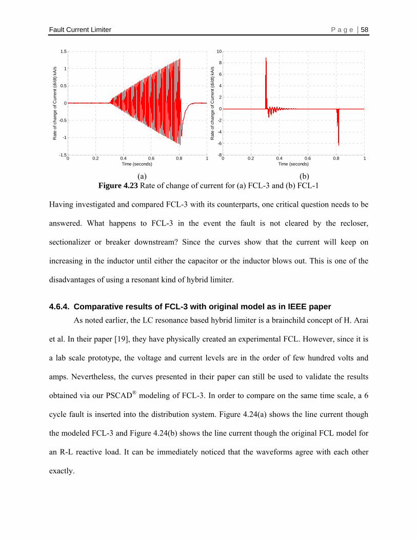
Fault Current Limiter P a g e | 58
0 0.2 0.4 0.6 0.8 1-1.5
-1
-0.5
0
0.5
1
1.5
Time (seconds)
Rat
e of
cha
nge
of C
urre
nt (d
i/dt)
kA/s
0 0.2 0.4 0.6 0.8 1-8
-6
-4
-2
0
2
4
6
8
10
Time (seconds)
Rat
e of
cha
nge
of C
urre
nt (d
i/dt)
kA/s
(a) (b)
Figure 4.23 Rate of change of current for (a) FCL-3 and (b) FCL-1 Having investigated and compared FCL-3 with its counterparts, one critical question needs to be
answered. What happens to FCL-3 in the event the fault is not cleared by the recloser,
sectionalizer or breaker downstream? Since the curves show that the current will keep on
increasing in the inductor until either the capacitor or the inductor blows out. This is one of the
disadvantages of using a resonant kind of hybrid limiter.
4.6.4. Comparative results of FCL-3 with original model as in IEEE paper As noted earlier, the LC resonance based hybrid limiter is a brainchild concept of H. Arai
et al. In their paper [19], they have physically created an experimental FCL. However, since it is
a lab scale prototype, the voltage and current levels are in the order of few hundred volts and
amps. Nevertheless, the curves presented in their paper can still be used to validate the results
obtained via our PSCAD® modeling of FCL-3. In order to compare on the same time scale, a 6
cycle fault is inserted into the distribution system. Figure 4.24(a) shows the line current though
the modeled FCL-3 and Figure 4.24(b) shows the line current though the original FCL model for
an R-L reactive load. It can be immediately noticed that the waveforms agree with each other
exactly.

Fault Current Limiter P a g e | 59
0.3 0.35 0.4 0.45-8
-6
-4
-2
0
2
4
6
8
10
Time (seconds)
Line
cur
rent
(kA rm
s)
CurrentFault
(a) (b)
Figure 4.24 Line current through (a) FCL-3 and (b) original model [19] Similarly, Figure 4.25(a) shows the voltage waveform across FCL-3 and Figure 4.25(b) shows
for the original model. The waveforms are almost similar. From Figure 4.25(a) and (b) it can be
seen that the FCL creates a very high pulse voltage when the fault is removed and eventually
reaches steady state in about 5 cycles. It is important to note that this pulse can be almost 6 times
the bus voltage. In order to mitigate those effects, a metal oxide surge arrestor can be employed.
0.3 0.35 0.4 0.45 0.5-80
-60
-40
-20
0
20
40
60
80
100
120
Time (seconds)
Line
Vol
tage
(kV
)
CurrentFault
(a) (b)
Figure 4.25 Voltage difference across FCL waveform (a) FCL-3 and (b) original model [19]
Fault Current Limiter P a g e | 60
Chapter 5. CONCLUSIONS AND FUTURE WORK This chapter provides an executive summary of the work presented in this thesis. Possible
future work is also discussed briefly.
5.1. Summary and Conclusions of thesis As it is evident now, FCL technology is still under development and at its infancy. Many
research papers and journals have proposed various methods to limit currents either by
simulation studies or by building lab scale prototypes. However, in most of the cases, there is
very little information on how the FCL modeling is actually done. As more professionals get
interested in this technology, it is important to create a general implementation methodology and
algorithm for developing an FCL. Hence, the work in this thesis can be summarized as follows:-
• First, a comprehensive and up-to-date literature review of the major kinds of fault
current limiters that have been simulated, lab tested and even installed in the field.
Results from a utility survey regarding advanced protection, adoption of FCL, and
upgrading activities, that was conducted as a part of the project is also reported. Current
status of the FCL technology along with potential issues and concerns are discussed.
• Second, proposed some of the techniques to model a behavioral fault current limiter in
the PSCAD® environment. This includes synthesizing of fault detection algorithms, FCL
activation, operation and timing and their respective algorithmic implementations.
• In particular, three types of FCL(s) were modeled, i.e. superconducting, solid state and
hybrid limiter.
Fault Current Limiter P a g e | 61
• A total of five case studies using the developed FCL models were conducted:-
The first three case studies involved using the superconducting FCL (FCL-1).
First, general results on a distribution system with and without an FCL were
discussed. It was shown that the use of FCLs in general can help in mitigating
currents while maintaining voltage stability and power. Also, the voltage drop
across the FCL pre/post fault was negligible. Second, a comparative study was
conducted between the modeled FCL-1 and the Z-energy model. It was shown
that without having access to proprietary manufacturer parameters, a generic
model can be created to behave in a similar fashion as that of real device. Finally,
the impact assessment on the protection scheme was carried out when an FCL is
inserted. It was reported that, when on average 85% current limitation is achieved,
the main sub-station re-closer will not “see” the fault even tough it is present.
The fourth study was conducted to study the operation and the behavior of a solid
state kind of limiter model (FCL-2). From simulation studies it was shown that,
by using power electronic switches, current can be commutated in a few
microseconds to the bypass reactor that limits the current. Also, it was learnt that
the use of a big enough inductor will not lead to un-necessary harmonics. As a
comparison, it was observed that during fault, FCL-2 produced a lower voltage
drop than FCL-1.
The final study was conducted to study the operation and the behavior of a LC
resonant based hybrid limiter model (FCL-3). From simulation studies it was
shown that, by using a superconducting coil and a capacitor in resonance can lead
Fault Current Limiter P a g e | 62
to a very slow and constant rate of change of current dtdi / during which the
main recloser or the substation down stream can clear the fault. Comparing this
limiter model to either FCL-1 or FCL-2, it was shown that upon fault insertion,
the current does not jump to a peak value in case of FCL-3 where as in FCL-1 or
2, the current peaked for about one cycle and then started limiting the current. In
addition, the curves obtained from FCL-3 modeling were compared to the actual
literature paper under which this model appeared. It was shown that both the
FCL-3 and the curves provided in the literature are the same.
Hence, it can now be concluded that the modeled FCL(s) worked as expected and produced
satisfactory results. This also shows that by creating a flexible model, parameters can be changed
at an instant and the effects of those changes can be monitored on a distribution system. This is
particularly useful when engineers are planning to evaluate new FCL technology in a particular
distribution system. This is the second major contribution of this thesis along with a
comprehensive literature review.
5.2. Future Work Future directions of this work include:-
• To run simulation studies with two or more FCL(s) in a larger distribution system, and
monitor its effect on current mitigation, relay co-ordination and possible mis-operation.
• Also, with increased interest in distributed generation and smart micro-grid technology,
it would be useful to evaluate the performance of the FCL in terms of current reduction
and directional sensing. With increase installation of DG, current can now travel in both
directions in a distribution system and the fault current contribution due to the
Fault Current Limiter P a g e | 63
distributed generator is also significant. There can be potential impacts on the directional
protection scheme and relay timing.
• As it was shown in the LC-resonant based hybrid limiter (FCL-3) that the current will
keep on increasing until a breaker clears the fault. A good extension of this would be
come up with an emergency control strategy that will effectively shut-off the FCL before
any damage happens to the device itself. Since, the behavior of FCL-3 is different from
FCL-1 or 2; it would be a good idea to assess its impact on the distribution protection
scheme and relay coordination.
• Another future work would be to create more FCL(s) in PSCAD® and add it to the
existing library of models that was created in this thesis. A simple drag-and-drop
approach will make the use of FCL model in system studies seamless and less time
consuming.
Fault Current Limiter P a g e | 64
References [1] G. Tang and M. R. Iravani, "Application of a Fault Current Limiter To Minimize
Distributed Generation Impact on Coordinated Relay Protection," International Conference on Power Systems Transients (IPST’05) in Montreal, Canada, 2005.
[2] V.A. Centeno, S.S. Venkata, P.Paretkar, D. Fan, M. Verma, S. Ming, and R. Phillips, "Literature Review of Fault Location, Prediction and Detection for Distribution Systems," p. 134, 02/14/2008 2008.
[3] J. A. Jiang, C. S. Chen, and C. W. Liu, "A New Protection Scheme for Fault Detection, Direction Discrimination, Classifi'cation, and Location in Transmission Lines," Power Engineering Review, IEEE, vol. 22, pp. 60-60, 2002.
[4] D. C. Elizondo and J. De La Ree, "Analysis of hidden failures of protection schemes in large interconnected power systems," in Power Engineering Society General Meeting, 2004. IEEE, 2004, pp. 107-114 Vol.1.
[5] W. G. D15, "High impedance fault detection technology," Report of Power System Relaying Committee, pp. 1-12, 1996.
[6] Barack Obama and J. Biden, "Barack Obama and Joe Biden: New Energy for America," pp. 1-8, 2008.
[7] E. M. Leung, "Superconducting fault current limiters," Power Engineering Review, IEEE, vol. 20, pp. 15-18, 30, 2000.
[8] W. Paul and M. Chen, "Superconducting control for surge currents," Spectrum, IEEE, vol. 35, pp. 49-54, 1998.
[9] A. T. Rowley, "Superconducting fault current limiters," The Institutuion of Electrical engineers 1995.
[10] G. G. Karady, "Principles of fault current limitation by a resonant LC circuit," Generation, Transmission and Distribution [see also IEE Proceedings-Generation, Transmission and Distribution], IEE Proceedings C, vol. 139, pp. 1-6, 1992.
[11] V. Sokolovsky, V. Meerovich, I. Vajda, and V. Beilin, "Superconducting FCL: design and application," Applied Superconductivity, IEEE Transactions on, vol. 14, pp. 1990-2000, 2004.
[12] J. Shi, J. Zou, and J. He, "Triggered-vacuum switch-based fault-current limiter," Power Engineering Review, IEEE, vol. 20, pp. 51-53, 2000.
[13] B. M. Ndeye K. Fall, "Fault Current Limiter – R&D Status and Testing Issues," in Power Engineering Society General Meeting, 2009. IEEE, 2009, p. 4.
Fault Current Limiter P a g e | 65 [14] Steve Eckroad, "Utility Needs Survey for Fault Current Limiters, EPRI," International
Workshop on Coated Conductors for Applications (CCA08), p. 7, December 4-6, 2008 2008.
[15] Manitoba HVDC Research Center, "PSCAD v4.2.1 On-Line Help System ", 2006.
[16] L. Masur, F. Darmann, and R. Lombaerde, "Design, Test and Demonstration of Saturable-Core HTS Fault current Limiter," Crystal City, VA: Z-energy, 2008.
[17] J. Vithayathil, "Power Electronics: Principles and Applications," PSCAD case file.
[18] F. Wanmin and Z. Yanli, "A novel IGCT-based Half-controlled Bridge Type Fault Current Limiter," in Power Electronics and Motion Control Conference, 2006. IPEMC '06. CES/IEEE 5th International, 2006, pp. 1-5.
[19] H. Arai, M. Inaba, T. Ishigohka, H. Tanaka, K. Arai, M. Furuse, and M. Umeda, "Fundamental Characteristics of Superconducting Fault Current Limiter Using LC Resonance Circuit," Applied Superconductivity, IEEE Transactions on, vol. 16, pp. 642-645, 2006.
[20] D. M. Farmer and K. H. Hoffman, "Application of Sectionalizers on Distribution Systems," in Rural Electric Power Conference, 2007 IEEE, 2007, pp. A2-A2-7.
[21] C. Williams, "Electronic Fuse Overcurrent Protection," in Transmission and Distribution Conference and Exhibition, 2005/2006 IEEE PES, 2006, pp. 1226-1228.
[22] Stanley H. Horowitz and A. G. Phadke, Power System Relaying, 2nd ed.: Research Studies Press LTD, 2000.
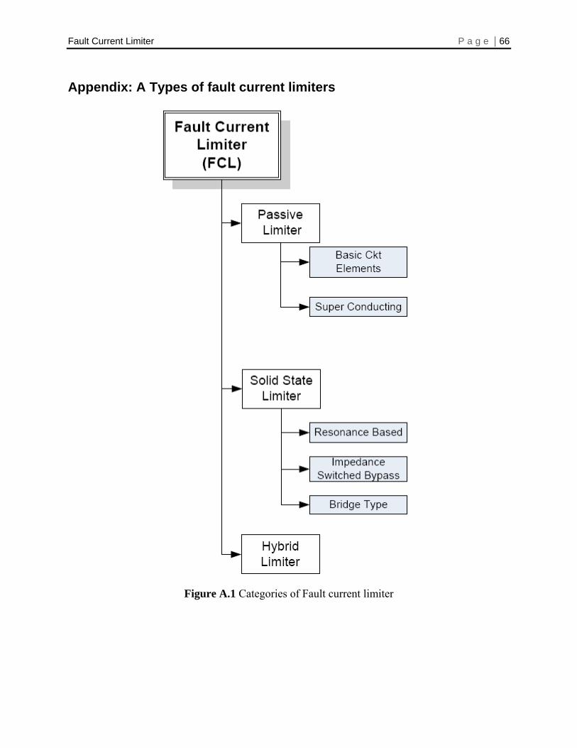
Fault Current Limiter P a g e | 66
Appendix: A Types of fault current limiters
Figure A.1 Categories of Fault current limiter
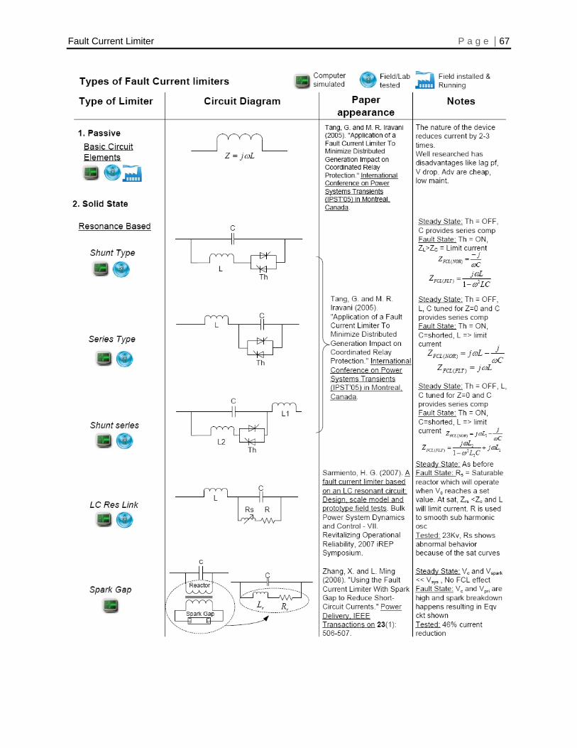
Fault Current Limiter P a g e | 67

Fault Current Limiter P a g e | 68
Figure A.2 Passive and Solid State limiters
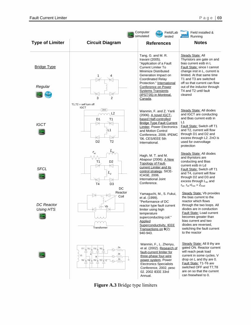
Fault Current Limiter P a g e | 69
Type of Limiter Circuit Diagram References Notes
T1
D3T4
D2
dL
acLacr
Bridge Type
1
23
4
DC Reactor Using HTS
DC Reactor
Coil
Vb
Transformer
SFCL
IGCT
Regular
Tang, G. and M. R. Iravani (2005). "Application of a Fault Current Limiter To Minimize Distributed Generation Impact on Coordinated Relay Protection." International Conference on Power Systems Transients (IPST’05) in Montreal, Canada.
Wanmin, F. and Z. Yanli (2006). A novel IGCT-based Half-controlled Bridge Type Fault Current Limiter. Power Electronics and Motion Control Conference, 2006. IPEMC '06. CES/IEEE 5th International.
Hagh, M. T. and M. Abapour (2006). A New Topology of Fault-current Limiter and its control strategy. SICE-ICASE, 2006. International Joint Conference.
Yamaguchi, M., S. Fukui, et al. (1999). "Performance of DC reactor type fault current limiter using high temperature superconducting coil." Applied Superconductivity, IEEE Transactions on 9(2): 940-943.
Wanmin, F., L. Zhenyu, et al. (2002). Research of fault-current limiter for three-phase four-wire power system. Power Electronics Specialists Conference, 2002. pesc 02. 2002 IEEE 33rd Annual.
Steady State: All Thyristors are gate on and bias current estb in LFault State: since I cannot change inst in L, current is limited. At that same time T1 and T3 are switched off so that current can flow out of the inductor through T4 and T2 until fault cleared
D1
T2D2
T1
ZnO
L1
L2
T1,T2 = self turn offIGCT
Steady State: All diodes and IGCT are conducting and Bias current estb in L1Fault State: Switch off T1 and T2, current will flow through D1 and D2 and excess through L2. ZnO is used for overvoltage protection
Steady State: All diodes and thyristors are conducting and Bias current estb in LdFault State: Switch off T1 and T4, current will flow through D2 and D3 and excess through Lac and rac. rac+Lac = Zload
T7 T1 T3 T5
T8 T4 T6 T2
L1 AB
C
Za
Zb
Zc
Steady State: All 8 thy are gated ON. Reactor current will reach peak load current in some cycles. V drop on L and thy are 0. Fault State: T1-T6 are switched OFF and T7,T8 are on so that the current can freewheel to 0.
Steady State: Vb provides the bias current to the reactor which flows through the two loops. All diodes are in conductionFault State: Load current becomes greater than bias current and two diodes are reversed, switching the fault current to the reactor
Computer simulated
Field installed &Running
Field/Lab tested
Figure A.3 Bridge type limiters
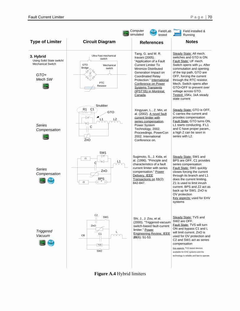
Fault Current Limiter P a g e | 70
Type of Limiter Circuit Diagram References Notes
3. HybridUsing Solid State switch/ Mechanical Switch
Triggered Vacuum
ZnO
CZ1
SW1
Z2BPS
L1
Series Compensation
L1
ZnO
L2
R1 C1
CSeries Compensation
Ultra Fast mechanicalswitch
GTO Bridge
Mechanicalswitch
PTC Resistor
GTO+Mech SW
Tang, G. and M. R. Iravani (2005). "Application of a Fault Current Limiter To Minimize Distributed Generation Impact on Coordinated Relay Protection." International Conference on Power Systems Transients (IPST’05) in Montreal, Canada.
Xingyuan, L., Z. Min, et al. (2002). A novel fault current limiter with series compensation. Power System Technology, 2002. Proceedings. PowerCon 2002. International Conference on.
Sugimoto, S., J. Kida, et al. (1996). "Principle and characteristics of a fault current limiter with series compensation." Power Delivery, IEEE Transactions on 11(2): 842-847.
Shi, J., J. Zou, et al. (2000). "Triggered-vacuum switch-based fault-current limiter." Power Engineering Review, IEEE20(6): 51-53.
Steady State: All mech. switches and GTO is ON.Fault State: UF mech. Switch opens with µs. After commutation and opening of the top path, GTO are OFF, forcing the current through the RTC resistor. Mech. Switch opens after GTO=OFF to prevent over voltage across GTO. Tested: 15Kv, 1kA steady state current
Snubber
GTOSteady State: GTO is OFF, C carries the current and provides compensationFault State: GTO turns ON, L1 starts conducting. If L1 and C have proper param., a high Z can be seen in series with L2.
TVS
C2
C1
ZnO
SW2
SW1
CBL
Steady State: TVS and SW2 are OFF. Fault State: TVS will turn ON and bypass C1 and L will limit current. ZnO is used for OV protection and C2 and SW1 act as series compensationKey aspects: TVS based devices
available for EHV systems and the
technology is reliable and fast to operate
Steady State: SW1 and BPS are OFF, C1 provides series compensationFault State: SW1 quickly closes forcing the current through its branch and L1 does the current limiting. Z1 is used to limit inrush current. BPS and Z2 act as back up for SW1. ZnO is OV protectionKey aspects: used for EHV systems
Computer simulated
Field installed &Running
Field/Lab tested
Figure A.4 Hybrid limiters
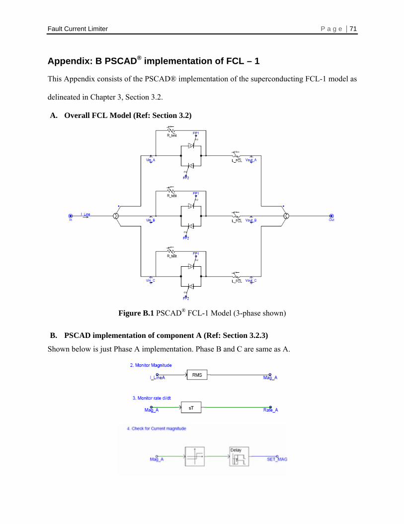
Fault Current Limiter P a g e | 71
x: B PSCAD® implementation of FCL – 1 Appendi
This Appendix consists of the PSCAD® implementation of the superconducting FCL-1 model as
delineated in Chapter 3, Section 3.2.
A. Overall FCL Model (Ref: Section 3.2)
Figure B.1 PSCAD® FCL-1 Model (3-phase shown)
B. PSCAD implementation of component A (Ref: Section 3.2.3)
Shown below is just Phase A implementation. Phase B and C are same as A.
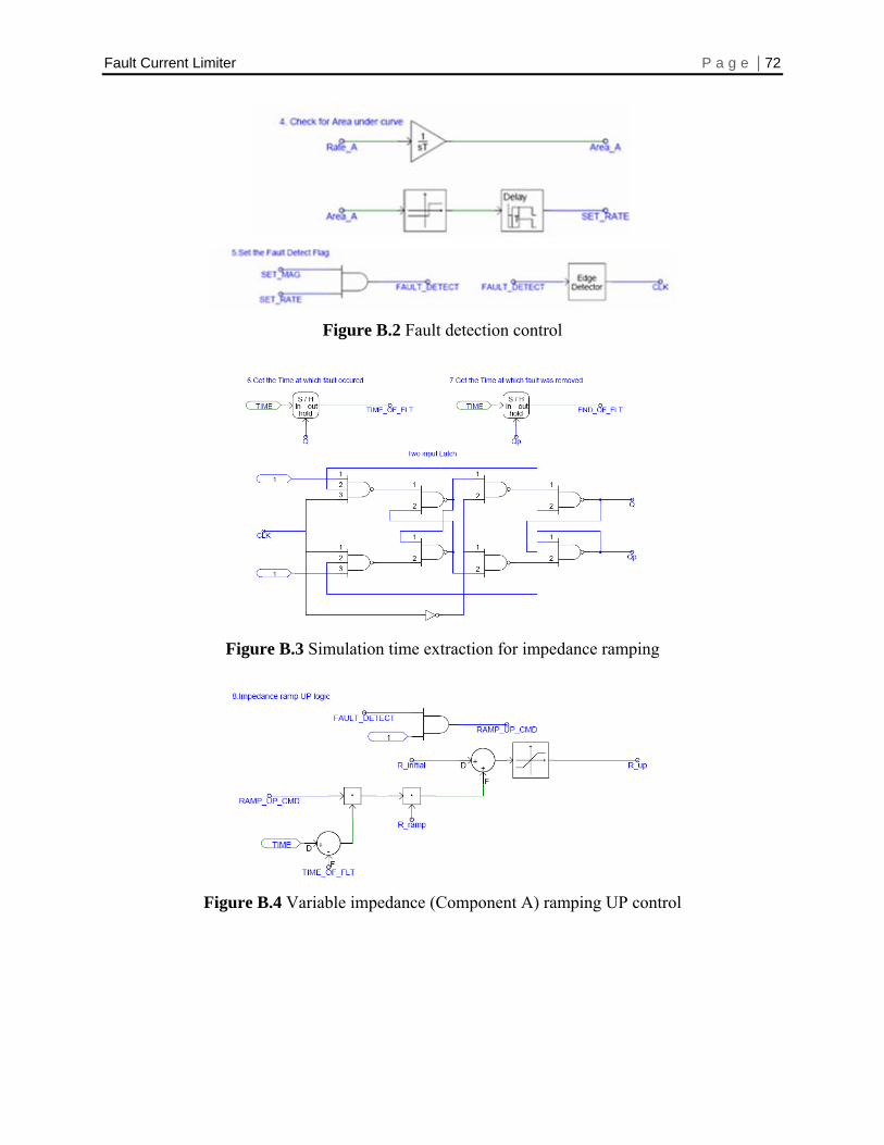
Fault Current Limiter P a g e | 72
Figure B.2 Fault detection control
Figure B.3 Simulation time extraction for impedance ramping
Figure B.4 Variable impedance (Component A) ramping UP control

Fault Current Limiter P a g e | 73
Figure B.5 Variable impedance (Component A) ramping DOWN control
Figure B.6 Final reference to the variable impedance (Component A)
C. PSCAD implementation of component B (Ref: Section 3.2.4)
Figure B.7 Thyristor Firing Control (Courtesy: PSCAD®)
D. PSCAD implementation for fault insertion (applicable to all simulation studies)
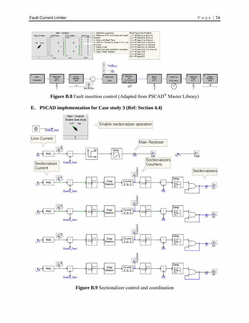
Fault Current Limiter P a g e | 74
Figure B.8 Fault insertion control (Adapted from PSCAD® Master Library)
E. PSCAD implementation for Case study 3 (Ref: Section 4.4)
Figure B.9 Sectionalizer control and coordination
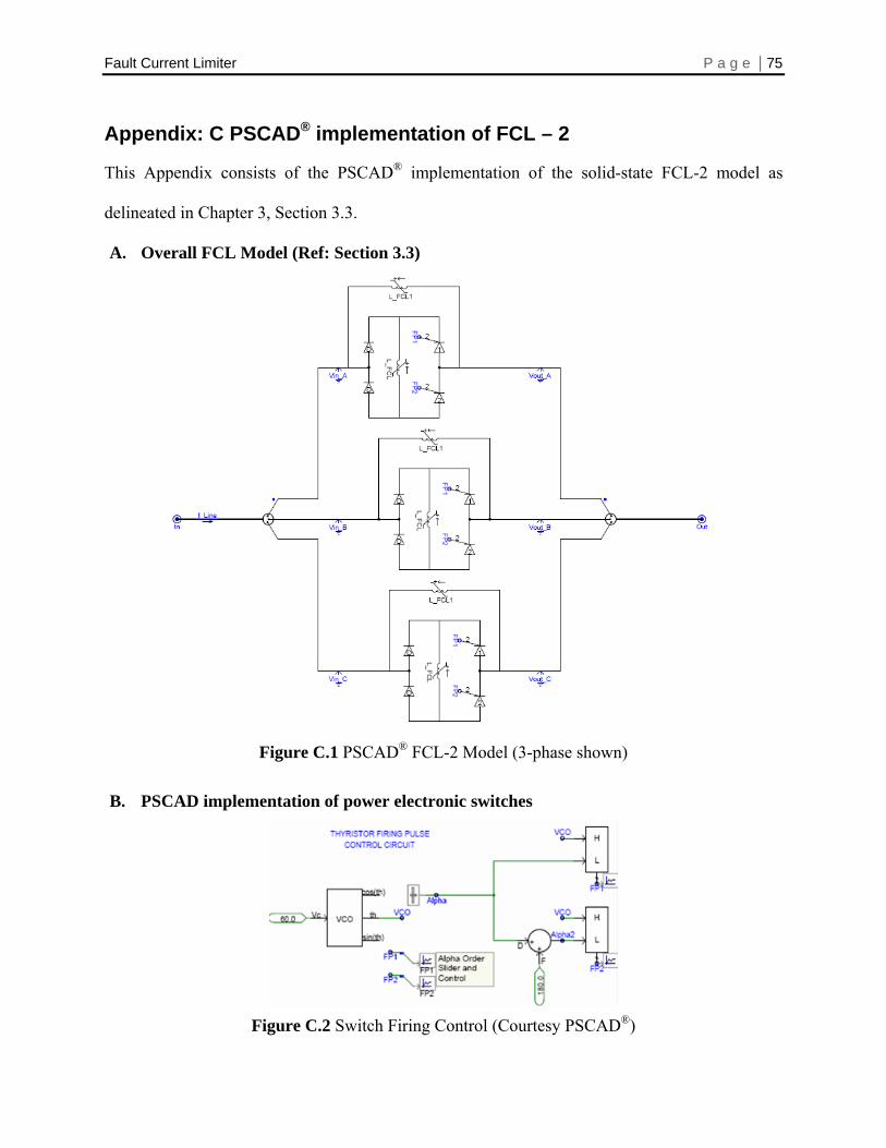
Fault Current Limiter P a g e | 75
x: C PSCAD® implementation of FCL – 2 Appendi
This Appendix consists of the PSCAD® implementation of the solid-state FCL-2 model as
delineated in Chapter 3, Section 3.3.
A. Overall FCL Model (Ref: Section 3.3)
Figure C.1 PSCAD® FCL-2 Model (3-phase shown)
B. PSCAD implementation of power electronic switches
Figure C.2 Switch Firing Control (Courtesy PSCAD®)
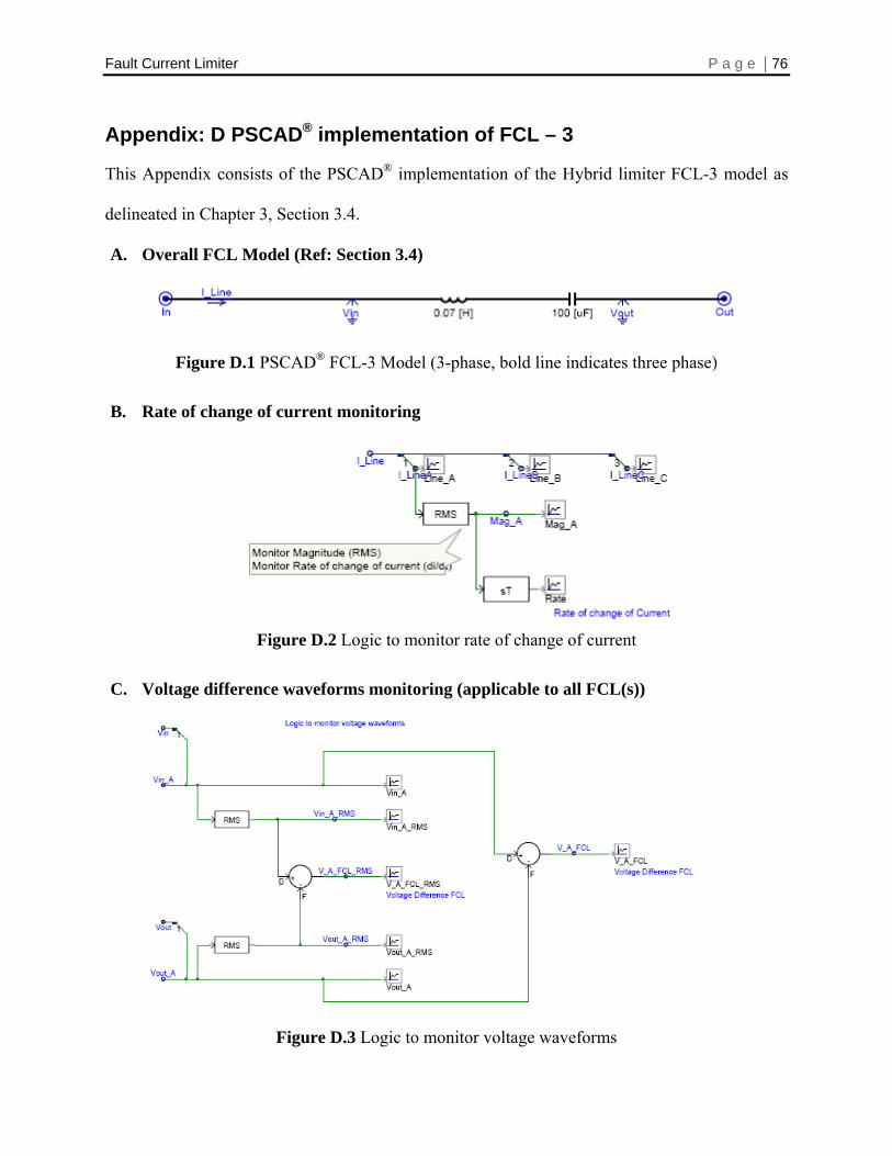
Fault Current Limiter P a g e | 76
Appendi
This Appendix consists of the PSCAD® implementation of the Hybrid limiter FCL-3 model as
delineated in Chapter 3, Section 3.4.
C. Voltage difference waveforms monitoring (applicable to all FCL(s))
B. Rate of change of current monitoring
A. Overall FCL Model (Ref: Section 3.4)
Figure D.1 PSCAD® FCL-3 Model (3-phase, bold line indicates three phase)
x: D PSCAD® implementation of FCL – 3
Figure D.2 Logic to monitor rate of change of current
Figure D.3 Logic to monitor voltage waveforms
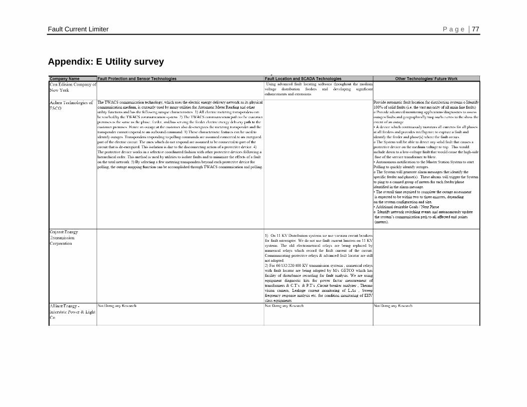
Fault Current Limiter P a g e | 77
Appendix: E Utility survey
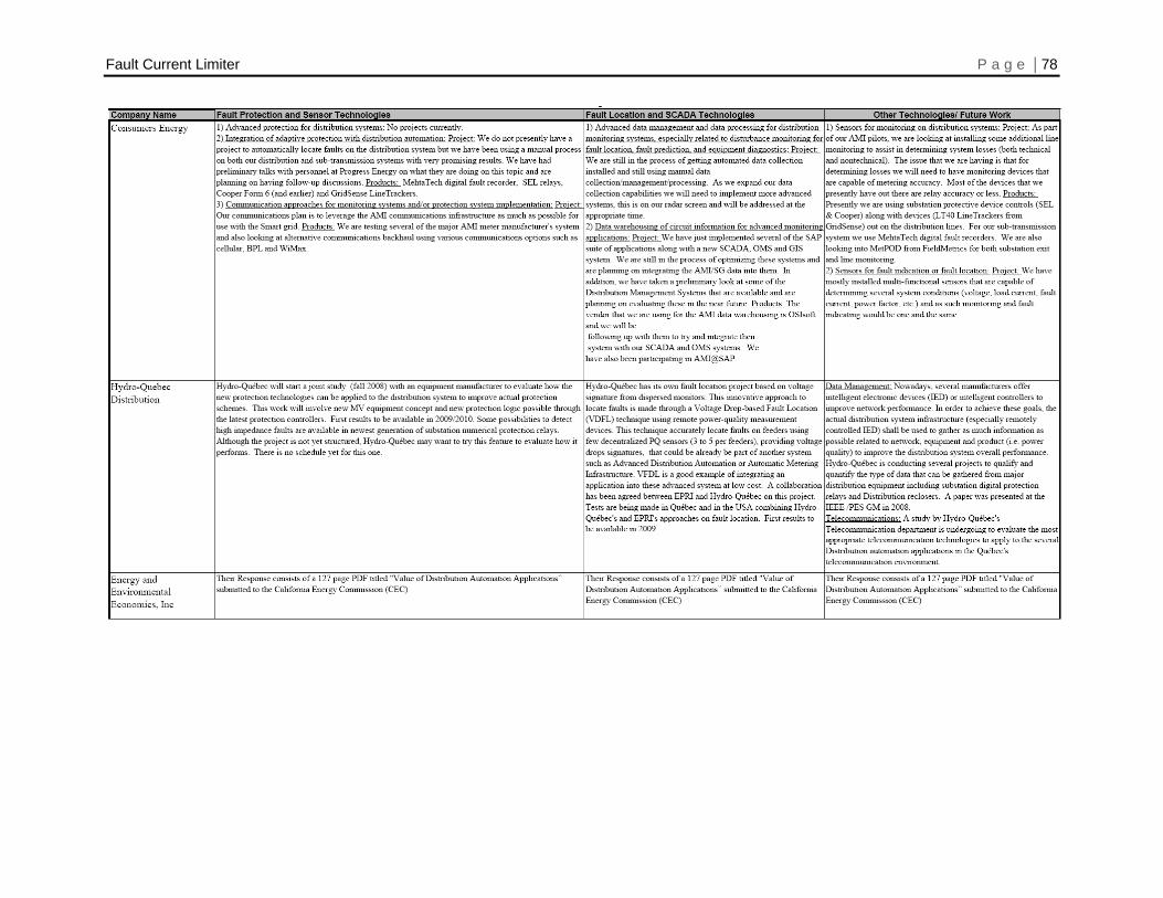
Fault Current Limiter P a g e | 78
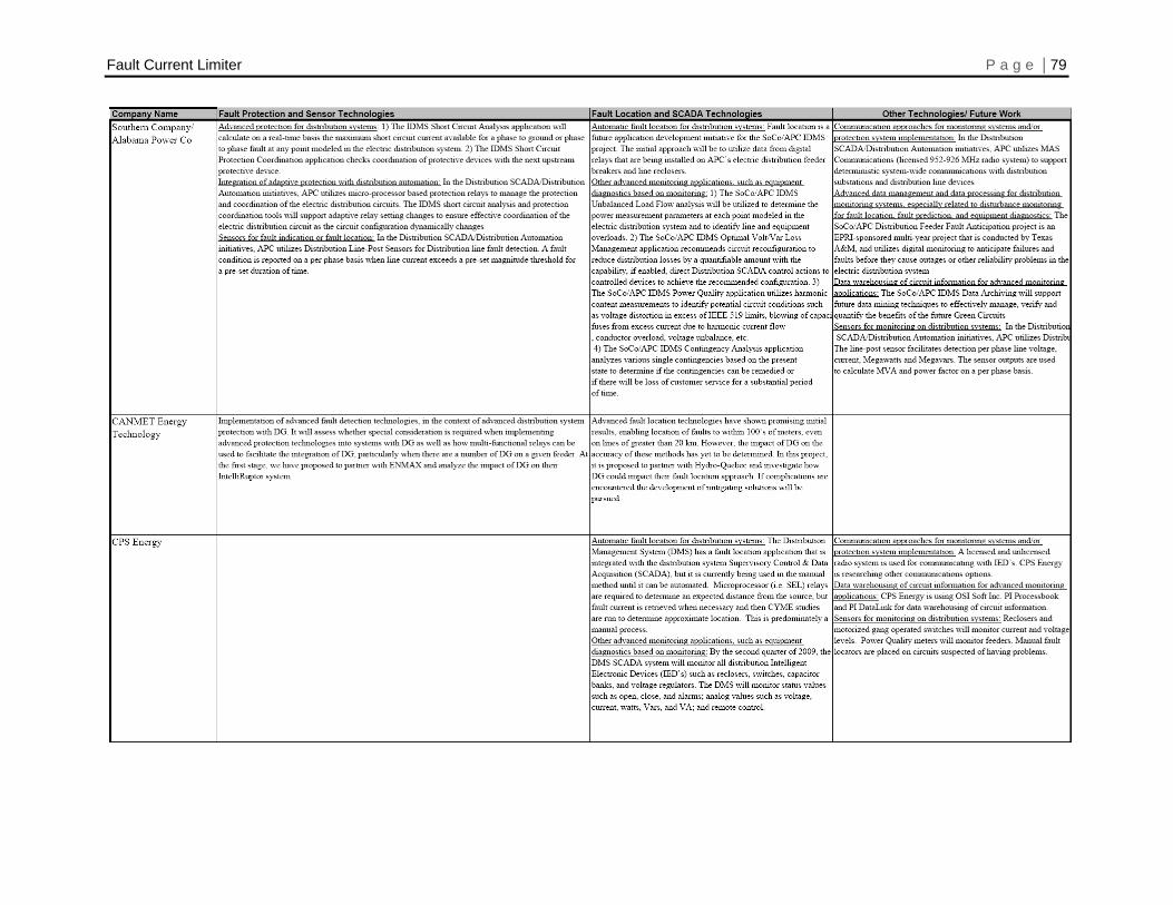
Fault Current Limiter P a g e | 79
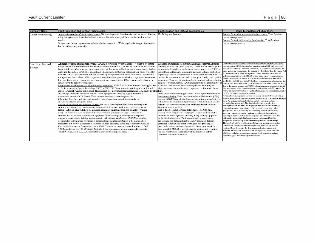
Fault Current Limiter P a g e | 80
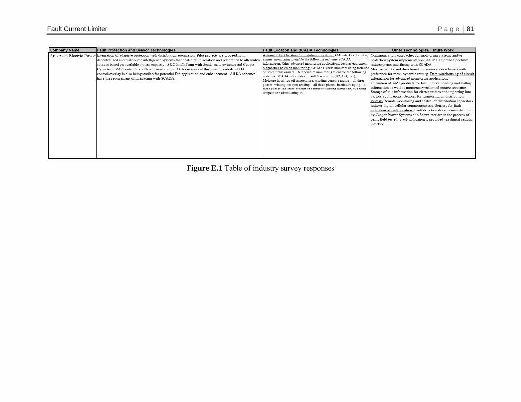
Fault Current Limiter P a g e | 81
Figure E.1 Table of industry survey responses