A comparison of trace-sampling techniques for multi

664

Cache I:. (Space)

Sets

1

IEEE TRANSACTIONS ON COMPUTERS, VOL. 43, NO. 6. JUNE 1994

. . . . . . . . . . . . . . . . . ;. . ~. .X . . iX X -5.. . . . . .. . . -. . . . . . . . . -. . . . . 1 : x i x x

Horizontal Slice x x x j

X x:x x ~

x x X

x :

A Comparison of Trace-Sampling Techniques for Multi-Megabyte Caches

R. E. Kessler, Mark D. Hill, and David A. Wood

Abstract-This paper compares the trace-sampling techniques of set sampling and time sampling. Using the multi-billion- reference traces of Borg et uL, we apply both techniques to multi-megabyte caches, where sampling is most valnable. We evaluate whether either technique meets a 10% sampling goal: a method meets this goal if, at least 90% of the time, it estimates the trace’s true misses per instruction with 5 10% relative error ’ using <_ 10% of the trace. Results for these traces and caches show that set sampling meets the 10% sampling goal, while time sampling does not. We also find that cold-start bins in time samples is most effectively reduced by the technique of Wood et al. Nevertheless, overcoming cold-start bias quires tens of millions of consecutive references.

Index rem-Cache memory, cache performance, cold start, computer architecture, memory systems, performance evaluation, sampling techniques, trace-driven simulation.

I. INTRODUCTION

OMPUTER designers commonly use trace-driven sim- C ulation to evaluate alternative CPU caches [21]. But as cache sizes reach one megabyte and more, traditional trace- driven simulation requires very long traces ( e g , billions of references) to determine steady-state performance [4], [22]. But long traces are expensive to obtain, store, and use.

We can avoid simulating long traces by using trace- sampling techniques. Let the cache performance of a small portion of the trace be an observation and a collection of observations be a sample. Sampling theory tells how to predict cache performance of the full trace, given a sample of unbiased observations [5], [ 141. With additional assumptions, we can also estimate how far the true value is likely to be from the estimate.

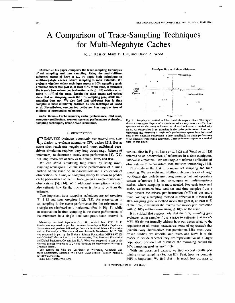
Two important trace-sampling techniques are set sampling [7], [18] and time sampling [12], [13]. An observation in set sampling is the cache performance for the references to a single set (depicted as a horizontal slice in Fig. l), while an observation in time sampling is the cache performance of the references in a single time-contiguous trace interval (a

Manuscript received September 31, 1991; revised June 1993. R. E.

Time-Space. Diagram of Memory References

x x .........-.....

I X

Time

Fig. 1. Sampling as vertical and horizontal time-space slices. This figure shows a time-space diagram of a simulation with a very short trace.lhe time (position within the trace) and cache set of each reference is marked with an X . An observation in set sampling is the cache performance of one set. References that determine a single set’s performance appear inan horizontal slice of this figure.An observation in time sampling is the cache performance of an intervalof consecutive references. These references appear in a vertical slice of this figure.

vertical slice in Fig. 1). Laha et ai. [12] and Wood et al. 1251 referred to an observation of references in a time-contiguous interval as a “sample.” We use sample to refer to a collection of observations to be consistent with statistics terminology [ 141.

This study is the first to compare set sampling and time sampling. We use eight multi-billion-reference traces of large workloads that include multiprogramming but not operating system references [4], and concentrate on multi-megabyte caches, where sampling is most needed. For each trace and cache, we examine how well set and time samples from a trace predict the misses per instruction (MPI) of the entire trace. We say a sampling method is effective if it meets the 10% sampling goal: a method meets this goal if, at least 90% of the time, it estimates the trace’s true misses per instruction with 5 10% relative error using 5 10% of the trace.

It is critical that readers note that the 10% sampling goal evaluates using samples from a trace to estimate that trace’s MPI. We do not formally address how our traces relate to the

Kessler was supported in Part by a Summer internship at Digital Equipment Corporation and graduate fellowships from the National Science Foundation

was supported in part by the National Science Foundation (MIPS8957278 and CCR-8902536). A.T.& T. Bell Laboratories, Cray Research Foundation and Digital Equipment Corporation. D. A. Wood was supported in part by the National Science Foundation (CCR-9 157366) and the University of Wisconsin Graduate School.

population of all traces, because we know of no research that

driven studies, we describe Our traces and leave it to the and the University of Wisconsin Alumni Research Foundation, M, D, Hill quantitatively characterizes that popu1ation’ Like most trace-

reader to decide whether they are representative of a larger population. Section discusses the reasoning behind the 10% samDling goal in more detail. . - -

The authors are with the University of Wisconsin, Computer sciences Department, Madison, WI 53706 USA; e-mail: { kessler, markhill, david) @cs.wisc.edu.

With our traces and caches, we find several results per- taining to set sampling (Section 111). First, how we compute

IEEE Log Number 9401099. MPI is important. We find that it is much less accurate to

0018-9340/94$04.M) 0 1994 IEEE

mailto:cs.wisc.edu

KESSLER cf a/.: A COMPARISON OF TRACE-SAMPLING TECHNIQUES FOR ML'LTI-MEGABYTE CACHES

normalize misses by the instruction fetches to the sampled set5 than by the fraction of sampled sets times all instruction fetches. Second, instead of selecting the sets in a sample at random, selecting sets that share several index bit values reduces simulation time, facilitates the simulation of cache hierarchies, and still accurately predicts the trace's MPI. Third, and most important, set sampling is effective. For our traces and caches, it typically meets the 10% sampling goal.

For time-sampling (Section IV), we first compare techniques for overcoming cold-start bias [6], Le., determining the MPI for a particular trace interval without knowing the initial cache state. We consider leaving the cold-start bias unchanged, recording metrics only during the second half of each interval, recording metrics only for initialized sets [12], [22], stitching intervals together [ 11, and Wood er ul.'s model for predicting the initialization reference miss ratio [25]. For our traces and caches, we obtain two results. First, on average, the technique of Wood et al. minimizes the cold-start bias better than the other techniques. Second, for the multi-megabyte caches we Ftudied, interval lengths of tens of millions of instructions and larger are needed to reduce the effects of cold-start.

Then using Wood et al.'s technique to mitigate cold-start bias, we find that time sampling fails to meet the 10% sampling goal for our traces and caches, because: 1) many intervals are needed to capture workload variation, and 2) long intervals are necessary to overcome cold-start bias. As a result, for these traces and caches, set sampling is more effective than time sampling for estimating MPI. Set sampling is not appropriate, however, for caches with time-dependent behavior (e.g., prefetching) or interactions between sets (e.g., a single write buffer).

We do not consider other (non-sampling) techniques that reduce trace data storage, such as, Mache [ 191, stack deletion and snapshot method [20], trace (tape) stripping [18], [231, or exploiting spatial locality [2]. These techniques can be used in addition to the sampling considered in this study. We also do not consider Przybylski's prefix technique [16], which prepends all previously-referenced unique addresses to each time-observation. This method seems unattractive for multi- megabyte caches where each time-observation requires its own prefix and each prefix must be very large for programs that can exercise multi-megabyte caches.

11. METHODOLOGY This section describes the traces, caches, and performance

metric we use in later sections.

A. The Truces

The traces used in the study were collected at DEC Westem Research Laboratory (WRL) [3], [4] on a DEC WRL Titan [ 151, a loadstore ("RISC") architecture. Each trace consists of the execution of three to six billion instructions of large workloads, including multiprogramming but not operating system references. The traces of the multiprogrammed workloads represent the actual execution interleaving of the processes on the traced system. The traces reference from eight to over one hundred megabytes of unique memory locations. These traces are sufficiently long to overcome the cold-start

TABLE I A DESCRIPTIO% OF THE STLlDlED WORKLOADS

665

Dcxnption

A muluprogram aorkload con\!sting of (I) Make C campilmg portions of the Magic source code. ( 2 ) Cirr routing the DEC%ation 3100 Printed Circuit Board (16 megabytes). ( 3 ) Magic Dectgn Rule Checking the MulttTitan CPU chip (20 megabytes). (4) Tree given 10 megahytec of working space solving the same problem as the Tree workload, (5) another Makc that largely consists of a call to Xld to load the Magic ohject code (2C megabytes). and ( 6 ) an infinite loop shell of interactive Unix commands ( cp. cat. ex, rm pc -aux, Is -I /* 1 The trace skipped ahout the first billion instructions so the larger programs. Grr, Magic. Tree, and Xld. were able to initialize their large data structures and start using them. The p n r e s \witch interval WdS approximately 200.000 instruction cy- des

Thc same workload a\ Mult l except the procev switch interval i c approximately 4 W . m hasic ~ n s t ~ c t i o n cyclm

The Mul t l workload excluding the Xld (Make) run (5) and the Tree program (4). Mu112 has a lower degree 01 multiprogramming and i s smaller than Mul t l

'The same workload a\ Mu112 except the process w i t ch interval is approximately 400,000 hasic Initruction cycle\.

A uniprogram workload uf Tv analyiing the timing of the DEC WRL MultiTitan CPU chip Tv required 12.5 hillion instructions to complete the timing analysis. About the first IO hillion in\tmction\ huild B very large linked data stmcture. The final 2-3 hillion inclructions traverse the structure. The end of the execution of Tv was captured on rape.

A uniprogram u,orklnad of the Sor program doing matrix manipulations on a 800,Mx) by 2LNl.MX) spane matrix with approximately 4 million (0.0325%) of the matrix entries k- ing nun-zero About thc hrnt hillion IIISIN~~IOPS create the large matrices. The rest 01 the program 1s the matrix upcralions. The trace captures a portion of the matrix opera- tions. excluding initialization.

k uniprogram workload consisting of the Tree program. Tree has two major phases that were traced. Ahout the first ha l f of the instructions build a large tree suucturc that repreqenls a Unix-like hierarchical directory structure. The rest o f the instructions search this tree to find the largest memkr

A uniprogram workload of Linear analyzing the power supply of a register file Normal- '

ly, the program tries to minimize the amount of work it must do by combining circuit ~

structures. The trace was collected hy disabling some of these comhinmg operation\ to

--

_ _ _ _ _ _ _ _ ~ ~ ~ ~ ~ ~

____.

~ ~~

~-

~ ~ ~ _ _ ~ ~ _ _

produce a bigger problem, possibly reflecting the larger pmhlems of the future. i

This table consists of a description of the user-only (no kernel references) workloads used in this study. Four workloads are uniprogrammed and two are multiprogrammed workloads. The uniprogrammed workloads consist of the largest programs. Several smaller programs were grouped with some standard Unix programs to produce the multiprogrammed workloads.

intervals of even the large caches considered in this study. We chose programs with large memory requirements because of the likelihood that large application sizes will become more common as main memories of hundreds of megabytes become available.

Table I describes traces in detail. The Mult2 trace includes a series of compiles, a printed circuit board router, a VLSI design rule checker. and a series of simple programs commonly found on UNIXTM systems, all executing in parallel (about 40 megabytes active at any time) with an average of 134 000 instructions executed between each process switch. The Mult2.2 trace is the Mult2 workload with a switch interval of 2 14 000 instructions. The Multl trace includes the processes in the Mult2 trace plus an execution of the system loader (the last phase of compilation) and a Scheme (Lisp variant) program (75 megabytes active) and has a switch interval of 138000 instructions. The Multl.2 trace is the Multl workload with a switch interval of 195 000 instructions. The Tv trace is of a VLSI timing verifier (96 megabytes). Sor is a uniprocessor successive-over-relaxation algorithm that uses large, sparse matrices (62 megabytes). Tree is a Scheme program that searches a large tree data structure (64 megabytes). Lin is a power supply analyzer that uses sparse matrices (57 megabytes).

B. Criche Assirmptions

This study focuses on multi-megabyte unified (both instructions and data cached together) caches. Earlier work has shown

T\I Trademark AT&T Bell I.aboratorieq.

666

that both techniques are effective for smaller caches [12], [18]. We vary the size and set-associativity of these caches over a range of sizes from 1-megabyte to 16-megabytes and associativities from direct-mapped to four-way. The caches do no prefetching, use write-back and write-allocate policies, and have 128-byte blocks. The caches use virtual-indexing (i.e., select the set of a reference using the reference’s virtual address) with PID-hashing, an approximation to real-indexing. PID-hashing means that we exclusive-or the upper eight index bits from the virtual address with the process identifier (PID) of the currently executing process. We also examined several real-indexed caches and found that they produced results similar to those in this paper, which is not surprising since real-indexed cache performance is often close to virtual- indexed cache performance. The non-direct-mapped caches . use a random replacement policy, which was easier to handle in the our simulation environment than is least-recently-used replacement.

Since multi-megabyte caches are likely to be used in a cache hierarchy, we simulate them as alternative secondary caches placed behind a fixed primary cache. The primary caches are split (separate) instruction and data caches that are 32-kilobytes each, direct-mapped, 32-byte blocks, do no prefetching, use virtual indexing, and write-back and write- allocate policies. We do not evaluate primary cache tradeoffs in this study since secondary cache performance is unaffected by the primary caches when their sizes differ by at least a factor of eight [17].

C. The Performance Metric: Misses Per Instruction

We measure cache performance with misses per instruction (MPI) rather than miss ratio. For comparing the performance of alternative unified secondary caches, MPI is equivalent to Przybylski’s global miss ratio [ 171. Specifically, a cache’s MPI is equal to its global miss’ratio times the average number of processor references (instruction fetches and data references) per instruction.

D. The 10% Sampling Goal

Given a particular trace and cache, let MPItrue be MPI obtained by simulating the complete trace with an initially empty cache (the true MPI of the complete trace). We say a sampling method is effective (for that trace and cache) if it meets the following goal:

Defiition I) 10% Sampling Goal: A method meets the IO% sampling goal if, at least 90% of the time, it estimates the trace’s true misses per instruction with 5 10% relative error using 5 10% of the trace.

The IO% sampling goal evaluates using samples from a trace to estimate MPItrue (that trace’s MPI). As discussed in the introduction, we do not formally address how our traces relate to the population of all traces, because we know of no research that quantitatively characterizes that population. For this reason, readers must choose between accepting our results (by assuming our traces are representative of their workload) and re-applying our techniques to their traces. We share this

IEEE TRANSACTIONS ON COMPUTERS, VOL. 43, NO. 6, JUNE 1994

failure of generalizing to the population of all traces with all trace-driven cache studies we are aware of.

We chose 5 10% of the references in a trace and 5 10% relative error using our experience with cache design and evaluation. We expect cache designers would not confront the intellectual complexity of sampling for less than a factor of ten reduction in trace size. We also expect many cache designers would consider negligible a 10% relative error in estimating a trace’s MPI, since MPI variations between traces often exceed factors of ten. Nevertheless, other cache designers may wish to choose stricter or looser criteria and re-apply the techniques described in this paper.

111. SET SAMPLING

We first examine set sampling, where an observation is the MPI of a single set and a sample is a collection of single- set observations. Section 111-A discusses how to compute a set sample’s MPI and why it should not contain random sets, while Section 111-B examines how well set sampling predicts MPItrue, the MPI of a full trace.

A. Constructing Set Samples In this section, we find

that how we compute MPI is important; specifically, it is much less accurate to normalize misses by the instruction fetches to the sampled sets than by the fraction of sampled sets times all instruction fetches. Consider a cache with s sets. For each set i , let miss, and instrn, be the number of the misses and instruction fetches to set i. Let S be a sample containing all references to n sets.

We consider two ways to calculate the MPI of sample S. =IS, which both require two counters to process a trace. Both use one counter to accumulate the number of the misses to the sets in the sample. At the end of the trace, this counter equals EzES miss,.

The sampled-instructions method uses the second counter to accumulate the instruction feEhes to the sets in the sample (EzES instrn,) and computes MPIs with:

Calculating the MPI of a Sample:

h Lies miss; MPIs = CiEs instrn; ’

The fraction-instructions method uses the second counter to to accumulate the instruction fetcJhes to all sets in the cache (E:=’=, instrn;) and computes MPIs with:

h EiEs miss; MPIs = 7L

; E:==, instrn; .

An alternative view of the effort required for these two methods is to consider the information that must be saved from the full trace if cache simulation is not done when gathering the trace. Both methods require that all references to the sampled sets be saved. The fraction-instructions method also requires a count of the number of instruction fetches in the full trace. Since most trace-gathering tools accommodate adding a counter, we consider the difficulty of obtaining data for the two methods comparable.

h t S \ L t K cr ul A COMPARISON OF TRACE-SAMPLING TECHNIQUES FOR MULTI-MEGABYTE CACHES

Trace

661

Coefficient of Variation (percent) MP'ime IOGo ;action-instructions sampled-instructions

TABLE 11 COtttlCIENT OF VARIATION OF MPI COMPUTATIONS

Multl 2.3% 35.2% 1.9% 28.9% 1.9% 24.2% 1.3% 24.3% 0.6% 139.0% 0.3%

0.59 6.8% 0.09 1.6%

This table illustrates the accuracy of computing the full trace MPI (column two) for several traces with the fraction-instructions and sampled-instructions methods. The accuracy is evaluated with the coefficient of variation (Equation ( I ) ) for the MPI estimates from a 4-megabyte direct-mapped secondary cache with 16 set samples of 1/16 the full trace each. The set samples are constructed with the constant bits method described in the next section. Results show that the fraction-instructions method is far superior to the sampled-instructions method.

In addition, statistics for the fraction-instructions method are simpler than for sampled-instructions method. Since the frac.tion-itistructions method normalizes the number of misses by a constant (for a given sample size n and number of sets s), its MPI estimates can be handled as simple random.variables. MPI estimates for the sampled-instructions method, on the other hand, should be modeled as the ratio of two random variables.

We empirically compare the two methods by computing their coefficients of variation across all set samples S ( j ) obtained with the constant-bits method, a systematic sampling method described in Section 111-A-2:

where k = is the number of samples [5 , p. 2081. CV is the true coefficient of variation, because we compare the MPI's of all set samples from the finite population with the trace's true MPI. We do not compare the methods with expected error, c7,1(k@Is(j) - MPItrue), because the expected error of all set samples from the finite population is always zero.

Experimental results, illustrated in Table 11, show that the fraction-instructions method performs much better, never having a coefficient of variation more than one-tenth the sampled-instructions method. The difference is infinite for the Sor and Lin traces because loops confine many instruction fetches to a few sets.

We also investigated normalizing missi with total references per set and data references per set [IO]. These methods perform similarly to the sampled-instructions method and not as well as the fEtion-instructions method. We did not consider calculating MPIs with E. L E S miss, instrn, , because Puzak [ 181 showed estimating miss ratio with the arithmetic mean of the per-set miss ratios is inferior to dividing the misses to sampled sets by the references to sampled sets (the miss-ratio equivalent of the sampled-instructions method). For a sample containing all

Since the fraction-instructions method performed better than the other methods examined, we will use it for the obtaining the remaining set sampling results.

The Constunt-Bits Method: We now examine two methods for selecting sets to form a sample. We show why systematic

sets, Puzak's work also implies cf=, - # MPLrue.

filter with

\mulate each cache

- random ;i x t s o i

evchcack

simulate each cache

filter with four

C0"StMt

bits

(a) (b)

Fig. 2. Two methods for selecting the sets in a sample. This figure illustrates selecting sets for samples of three alternative caches (A, B, and C) using (a) random sets and (b) constant bits. When sets are selected at random, each simulation must begin by filtering the full trace. With constant-bits, on the other hand, a filtered trace can drive the simulation of any cache whose index bits contain the constant bits.

samples constructed via constunt-bits offer advantages over random samples.

Assume that we want to evaluate three caches with samples that contain about 1/16th the references in a full trace. Let the caches choose a reference's set with bit selection (i.e., the index bits are the least-significant address bits above the block offset) and have the following parameters:

Cache A: 32-kilobyte direct-mapped cache with 32-byte blocks (therefore its index bits are bits 14-5, assuming references are byte addresses with bit 0 being least-significant); Cache B: 1 -megabyte two-way set-associative cache with 128-byte blocks (index bits 18-7); and Cache C: 16-megabyte direct-mapped cache with 128-byte blocks (index bits 23-7). One method for selecting the sets in a sample is to choose

them at random [ 181. To evaluate cache A with references to random sets, we randomly select 64 of its 1024 sets (1/16th), filter the full trace to extract references to those sets. and then simulate cache A. For cache B, we select 128 of its 2048 sets, filter and simulate. Similarly for cache C, we use 8192 of its 131 072 sets. As illustrated in Fig. 2(a), selecting sets at random requires that each simulation begin by extracting references from the full trace. Furthermore, since primary and secondary caches usually have different sets, it is not clear how to simulate a hierarchy of cache when sets are selected at random.

A second method, which we call constant-bits, selects references rather than sets [22, p. 591. The constant-bits method forms a filtered trace that includes all references that have the same value in some address bits. This filtered trace can then be used to simulate any cache whose index bits include the constant bits2 [IO]. For example, if we filter a trace by retaining all references that have the binary value

'This description as~umes bir selection, Le., the set-indexing bits come directly from the address of the memory access [21]. The scenario is more complicated with other than simple bit-selection cache indexing. In particular, since we use PID-hashing in this study, we ensured that the hashed index bits did not overlap with the constant bits. Note that though we use virtual- indexing, one can apply the constant-bits technique to real-indexed caches. and to hierarchical configurations with both real and virtual indexed caches if the constant bits are below the page boundary.

668

Trace

Multl Multl.2 MultZ

Mult2.2 Tv Sor

Tree Lin

El M p , , ~ looo Fraction of Sets in Sample

1116 I I64

0.70 1.78 1.71 0.69 I .39 I .27 0.61 1.02 1 .so 0.59 1.85 I .% 1.88 1.94 0.74 7.54 26.05 19.45 0.59 0.94 0.99 0.09 1.26 I .35


sinm*lc TABLE 111 RANEOM SAMPLE VARIANCE OVER SYSTEMATIC SAMPLE VARIANCE

constant prim cache bits

Fig. 3. Using constant-bits samples with a hierarchy. This figure illustrates how to use constant-bits samples to simulate a primary cache (P) and three alternative secondary caches ( A , E and C).

!

oo00 (or one of the other 15 values) in address bits 11-8, then we can then use the filtered trace to select 1 4 6 4 of the sets in any cache whose block size is 256 bytes or less and whose size divided by associativity exceeds 2 kilobytes. These caches include caches A, B, and C, the primary caches used in this study (32-byte blocks, 32 kilobytes, direct-mapped) and all secondary caches (128-byte blocks, 1-16 megabytes, 1-4-way set-associative) considered in this paper.

Constant-bits samples have two advantages over random samples. First, as illustrated in Fig. 2(b), using constant- bits samples reduces simulation time by allowing a filtered trace to drive the simulations of more than one altemative cache. Second, constant-bits samples make it straightforward to simulate hierarchies of caches (when all caches index with the constant bits). As illustrated in Fig. 3, we may simulate the primary cache once and then use a trace of its misses to simulate alternative secondary caches.

One complexity of using constant-bits samples is that they are not random samples, since sets are selected systematically via certain bit patterns. Intuitively, constant-bits samples may work better than random samples if spreading the sampled sets throughout the cache captures more workload variation than selecting random sets. Constant-bits samples could perform worse than random samples, however, for workloads that use their address space systematically (e.g., frequent accesses to a large, fixed stride vector).

Cochran [5, ch. 81 develops a theory of systematic samples, which we review in Appendix A. Since the sample mean for both random and systematic samples are unbiased estimates of the population mean, systematic sampling yields more accurate estimates of the population mean if and only if the variance of the systematic sample mean is less than the variance of a random sample mean.

We examine this empirically in Table 111. For each trace with a 4-megabyte, direct-mapped cache, Table I11 displays the variance of the random sample mean divided by the variance of the systematic sample mean obtained with the constant bits method. Values greater than one indicate that systematic samples are more accurate than random samples; we see that systematic samples are more accurate or comparable to random samples in all cases.

1

Since the constant-bits method is easier to use than random samples and provides similar or better precision, we use the constant-bits method to construct set samples throughout the rest of this paper.

B. What Fraction of the Full Trace is Needed?

This section examines how well set samples estimate the MPI of a full trace. For reasons discussed above, we construct samples with the constant-bits method and calculate MPI estimate for a sample with the fraction-instructions method. We first look at the accuracy of set sampling when MPItrue is known; then we show how to construct confidence intervals for MPItrue when it is not known.

Table IV quantifies the error between set samples and MPItrue for several traces, direct-mapped cache sizes, and sample sizes. We measure errors with coefficient of variation calculated using (1). Table X in Appendix C gives the corresponding results for two-way set-associative caches.

The key result is that, for this data and for four-way set- associative caches not shown here, set sampling generally meets the 10% sampling goal. Consider the columns labeled "1/16" in Tables IV and X, which correspond to samples using 1/16th of the sets and therefore will contain less than 10% of the trace on average. Only Lin and Tree with 4-megabyte direct-mapped caches, marked with daggers, fail to have at least 90% of the constant-bits samples with relative errors of less than or equal to *lo%. (And they both have only 2 of 16 samples with more than *lo% relative error.) The data also show the set sampling performs well even if 1/64th of the sets are sampled.

We also observe that increasing associativity from direct- mapped to two-way reduces corresponding coefficients of variation by more than 50%. We conjecture that set sampling works better for two-way set-associative caches because they have fewer conflict misses than direct-mapped caches [8]. A high rate of conflict misses to a few sets can make those sets poor predictors of overall behavior.

Finally, in practical applications of set sampling, we want to estimate the error of an MPI estimate, using only the information contained within the sample (i.e., not using knowledge of MPItrue as did Tables IV and X). As Appendix B describes, we do this by calculating 90% confidence intervals, assuming

KtSFLFR eI 01 A COMPARISON OF TRACE-SAMPLING TECHNIQUES EOR MULTI-MEGABYTE CACHES 669

Trace Size

t IM 1 MulcI 4M

TABLE IV . SET SAMPLING PRECISION FOR DIRECT MAPPED

MPI,,", x loo0 s,,$060f Sets 1164 of Sets cv s f l o % cv I .55 16/16 4.3% N/A N/A 0.70 16/16 2.3% 62/64 4 8 6

MuIc1.2 4M 16M IM

Mu112 4M

16M I 033 I 16/16 1.6% I 64/64 2 % ~ IM I I45 I 16/16 29% I N/A N/A

0.69 16/16 1.9% 62/64 4.1% 0.32 16/16 1.5% 63/64 3.2% I .24 16/16 3.4% NIA N/A 0.61 16/16 1.9% 64/64 2.96

Sor 4M 16M IM

Tree 4M

16/16 1.3% 64/64 2.5% 16M 0.27 16/16 1.8% 64/61 3.4%

2.63 16/16 1.9% N/A NIA 4M 1.88 16/16 0.6% 64/64 2.1%

16M 1.03 16/16 0.6% 64/64 2.0% 16/16 0.4% N/A NIA

7.54 16/16 0.3% 64/61 0.7% I .97 16/16 0.0% 64/64 0.1% 2.16 15/16 5.6% NIA N/A 0.59 14/16 6.8% t 6/64 136% t

Lin 4M 16M

16M 1 030 I 15/16 4 1% I 61/64 65% IM 1 I16 I 16/16 33% I N/A N/A

0.09 14/16 7.6% t 54/64 15.0% t 0.02 16/16 0.3% 64/64 0.5%

~~

90% Confidence Intervals that Contain MP/,,,

1/64 of Sets Trace 1 Normal'? I 11160fSets I fraction percent fraction percent

Mull I Multl.2 Mulf2

Mult2.2 Tv Sor Tree Lin

yes

Yes

no yes no no

yes

yes

16/16 100% 16/16 100% 15/16 94% 16/16 100% 16/16 100% 16/16 100% 12/16 75% 16/16 100%

61/64 95% 60164 94% 61/64 95% 63/64 98% 51/64 78% 64/64 100% 47/64 73% 62/64 97%

I I I I I

For a 4-megabyte direct-mapped secondary cache and various traces and fraction of sets, this table gives the fraction and percent of 90% confidence intervals that contained MPIt,,,,. In all cases where the pefret MPI are normal, 90% confidence intervals usefully estimate how far MPI. is likely to he from MPI, r , , f ~ .

a) random samples and b) that our estimate of the mean is normally distributed. Since variance of observations within our systematic samples is often greater than variance of the population, assumption a) will tend make our confidence intervals larger than necessary. For finite populations, assumption b) will generally hold if the underlying population is not highly skewed [5, Section 2.1 11.

We empirically studied the usefulness of confidence intervals two ways. First, we tested the validity of assumption b) using normal scores plots (not shown) for sets of 4- megabyte direct-mapped caches [ 14, p. 1721. Results show that assumption b) is valid for the four multiprogramming traces (Mult 1, Mult 1.2, Mult2, and Mult2.2) and Sor, but not for Tv, Tree, and Lin. Tree and Lin both have several "hot sets," and these outliers significantly skew their distributions. This suggests that confidence intervals for uniprogrammed traces should not be considered meaningful without additional

evidence. Second, we examined how often the 90% confidence intervals actually included the true mean. Table V displays data for constant-bits set samples and a 4-megabyte direct-mapped cache. Results show that the true mean lies within the 90% confidence intervals of at least 90% of the samples for all traces where the normal approximation appears valid.

C. Advantages and Disadvantages o j Set Sampling

The most important advantage of set sampling is that, for our simulations, it meets the 10% sampling goal (Definition 1). Especially for the multiprogrammed traces, a set sample automatically includes references from many execution phases, so an individual sample can accurately characterize the MPI of a full trace, including its temporal variability. The reduced trace data requirements of set sampling allow for simulation of longer traces, and therefore more algorithmic phases, in a smaller amount of time. Besides the data reduction, set sampling also reduces the memory required to simulate a cache. A set sample containing I / I6 of the full trace needs to simulate only 1/16 of the sets.

Set sampling does have its limitations. Even with the constant bits method, the full trace must be retained if one wishes to study caches that do not index with the constant bits. Furthermore, set sampling may not accurately model caches whose performance is affected by interactions between references to different sets. The effectiveness of a prefetch into one set, for example, may depend on how many references are made to other sets before the prefetched block is first used. Similarly, the performance of a cache with a write buffer may be affected by how often the write buffer fills up due to a burst of writes to many sets.

IV. TIME SAMPLING

The alternative to set sampling is time sampling. Here an observation is the MPI of a sequence of time-contiguous references and is called an interval. Section IV-A discusses determining the MPI for a sample, while Section IV-B examines using a sample to estimate MPI for the full trace.

A. Reducing Cold-Start Bias in Time Samples

To significantly reduce trace storage and simulation time, we must estimate the true MPI for an interval without knowledge of initial cache state, i.e., the cache state at the beginning of the interval. This problem is simply the well-known cold-start problem applied to each interval [6].

The cold-start problem is a key difficulty for time sampling. Sampling theory assumes that a sample is collection of observations, where each observation gives the true value for some member of the population. Set sampling meets this assumption, because computing the true MPI of a set, given all references to the set. is straightforward. Due to the cold-start problem, however, statistics for time sampling are calculated with estimates of the MPI of each interval, rather than the true values of each interval. Any bias in the interval estimates will. of course, remain in all statistics, including the sample mean.

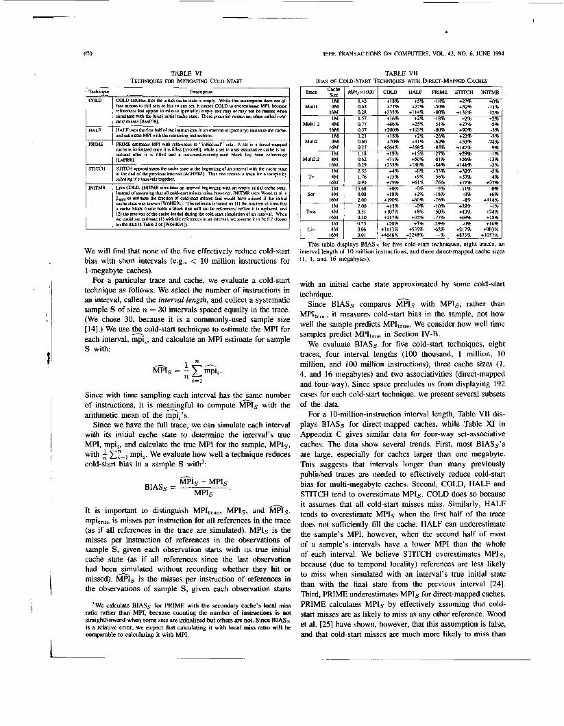
We compare how well the five techniques described in Table VI mitigate the cold-start problem in multi-megabyte caches.

7 I

Multl 4M 16M

670

0.62 +77% +27% -50% +52% - 1 1 % 0.28 +233% +114% -80% +I3146 -12%

TABLE VI TECHNIQUES FOR MITIGATING COLD-START

I Technique

16M IM

Sor 4M 16M

IM

De sc r i o t i o n

0.95 +79% 6 1 % -76% +7l% +37% +O% -0% -5% -11% 4% 15.68

8.08 +Il l% +2% -18% -8% +6% 2.00 +190% 4% -76% -8% +114% 2.00 +13% -040 -10% +29% -1%

COLD assumes hat Ihe initial cache state is empty. While this assumpion docs m af- fect misses to full sets or hits to any XI. it cauws COLD to overestimate MPI. bamae references thar a p p u to miss to (partially) empty sets may M may m he mi- when simulated with the (true) initial cache sfate. Thew potential misses are o f m called cold- smrt misses IE~sF781.

Tree 4M 16M

HALF uses the lint half of the instructions in an interval to (partially) initialire the cache. and estimates MPI with the remaining instructions.

0.51 +107% +8% -50% +43% +24% 0.30 +217% +35% -77% +69% +IS%

PRlME utimales MPI wilh references to "inmalircd" xu A set In a direct-mapped cache is inilialired once il is filled [STONWI. while a set tn a scl-assucialive cache IS in,- tialized after il IS Alled and a nun-musl-menilyuscd block has k n referenced

STITCH approximates the cache state at the beginning of an interval wilh he cache slaw a1 the end of thc prcviour interval IAoHH881 Thus one crcaies lrace for a sample h) srirrhing it's intervals togclhcr.

Like COLD. INITMR simulates an interval heginning wilh an empty initial cache slate lnsrcad of assuming h a l l cold-sm m i s s miss, houcrcr. INlTMR uscs W d et al:s fi-~,, lo eslimate the fraction of cold-sm misses that would have misxd if lhe initial cache state was known lWoHK911 The eslimate IS bascd on (I I the fraclion 01 lime !hat a cache block frame holds a block that will no1 be referenced heforc it IS replaced. and (2) the fraclion of the cache loaded dunng thc cold-sm simulation 01 an tnlerval. W k n we could not cstimale ( I ) with the references in an interval. we asume i t to he 0 7 ( b u d onthedatainTable2of [WoHK91]).

~- [LAP188].

Lin 4M 16M

We will find that none of the five effectively reduce cold-start bias with short intervals (e.g., < 10 million instructions for 1 -megabyte caches).

For a particular trace and cache, we evaluate a cold-start technique as follows. We select the number of instructions in an interval, called the interval length, and collect a systematic sample S of size n = 30 intervals spaced equally in the trace. (We chose 30, because it is a commonly-used sample size [ 141.) We use %cold-start technique to estimate the MPI for each interval, mpi,, and calculate an MPI estimate for sample S with:

- I n M P I ~ = - G i , .

n .

Since with time sampling each interval has the2ame number of instructions, it is meaningful to compute MPIs with the arithmetic mean of the mpi,'s.

Since we have the full trace, we can simulate each interval with its initial cache state to determine the interval's true MPI, mpi,, and calculate the true MPI for the sample, MPIs. with Cy=l mpi,. We evaluate how well a technique reduces cold-start bias in a sample S with3:

2=1

h

0.06 +I11396 +535% -62% +217% +903% 0.01 4 6 4 8 % +2248% -4% +873% +1037%

MTI~ - M P I ~ BIASs =

MPIs '

It is important to distinguish MPItrue, MPIs, and *IS. mpitrue is misses per instruction for all references in the trace (as if all references in the trace are simulated). MPIs is the misses per instruction of references in the observations of sample S, given each observation starts with its true initial cache state (as if all references since the last observation had been2mulated without recording whether they hit or missed). MPIs is the misses per instruction of references in the observations of sample S, given each observation starts

3We calculate BIASs for PRIME with the secondary cache's local miss ratio rather than MPI, because counting the number of instructions is not straightforward when some sets are initialized but others are nat. Since BIAS.5 is a relative error, we expect that calculating it with local miss ratio will be comparable to calculating it with MPI.

b


TABLE VI1 BIAS OF COLD-START TECHNIQUES WITH DIRECT-MAPPED CACHES

Trace I MPlsxlO0O I COLD HALF PRIME STKCH INITMR

IM I 1.45 I +18% +5% -18% +23% +O%

1.76 +15% +9% -56% +37% 4%

with an initial cache state approximated by some cold-start technique.

Since BIASs compares @IS with MPIs, rather than MPIt,,,, it measures cold-start bias in the sample, not how well the sample predicts MPIt,,,. We consider how well time samples predict MPItrue in Section IV-B.

We evaluate BIASs for five cold-start techniques, eight traces, four interval lengths (100 thousand, 1 million, 10 million, and 100 million instructions), three cache sizes (1, 4, and 16 megabytes) and two associativities (direct-mapped and four-way). Since space precludes us from displaying 192 cases for each cold-start technique, we present several subsets of the data.

For a 10-million-instruction interval length, Table VI1 displays BIASs for direct-mapped caches, while Table XI in Appendix C gives similar data for four-way set-associative caches. The data show several trends. First, most BIASs's are large, especially for caches larger than one megabyte. This suggests that intervals longer than many previously published traces are needed to effectively reduce cold-start bias for multi-megabyte caches. Second, COLD, HALF and STITCH tend to overestimate MPIs. COLD does so because it assumes that all cold-start misses miss. Similarly, HALF tends to overestimate MPIs when the first half of the trace does not sufficiently fill the cache. HALF can underestimate the sample's MPI, however, when the second half of most of a sample's intervals have a lower MPI than the whole of each interval. We believe STITCH overestimates MPIs, because (due to temporal locality) references are less likely to miss when simulated with an interval's true initial state than with the final state from the previous interval [24]. Third, PRIME underestimates MPIs for direct-mapped caches. PRIME calculates MPIs by effectively assuming that cold- start misses are as likely to miss as any other reference. Wood et al. [25] have shown, however, that this assumption is false, and that cold-start misses are much more likely to miss than

--

KESSLER et al.: A COMPARISON OF TRACE-SAMPLING TECHNIQUES FOR MULTI-MEGABYTE CACHES

, ’ Cache Interval COLD HALF PRIME STITCH INITMR

15 13 4

13 4 13

in x

Trace C;c; Mp,,,, looo Interval Length (Millions of Instructions) 1 in 100 0.1

4M

Muit1.2 IM 4M

16M Mull2 IM

4M

MuIt2.2 IM 4M

16M

16M

16M Tv 1M

Sor IM

Tree IM

4M 16M

4M 16M

4M 16M

Lin IM 4M

randomly-chosen references. PRIME is more accurate for four- way set-associative caches, where the heuristic of ignoring initial references to a most-recently-referenced block mitigates the underestimation. Fourth, INITMR did not consistently underestimate or overestimate MPIs. Finally, the large biases for the Lin trace with 4- and 16-megabyte caches are probably not important, because Lin’s true MPI’s are so small.

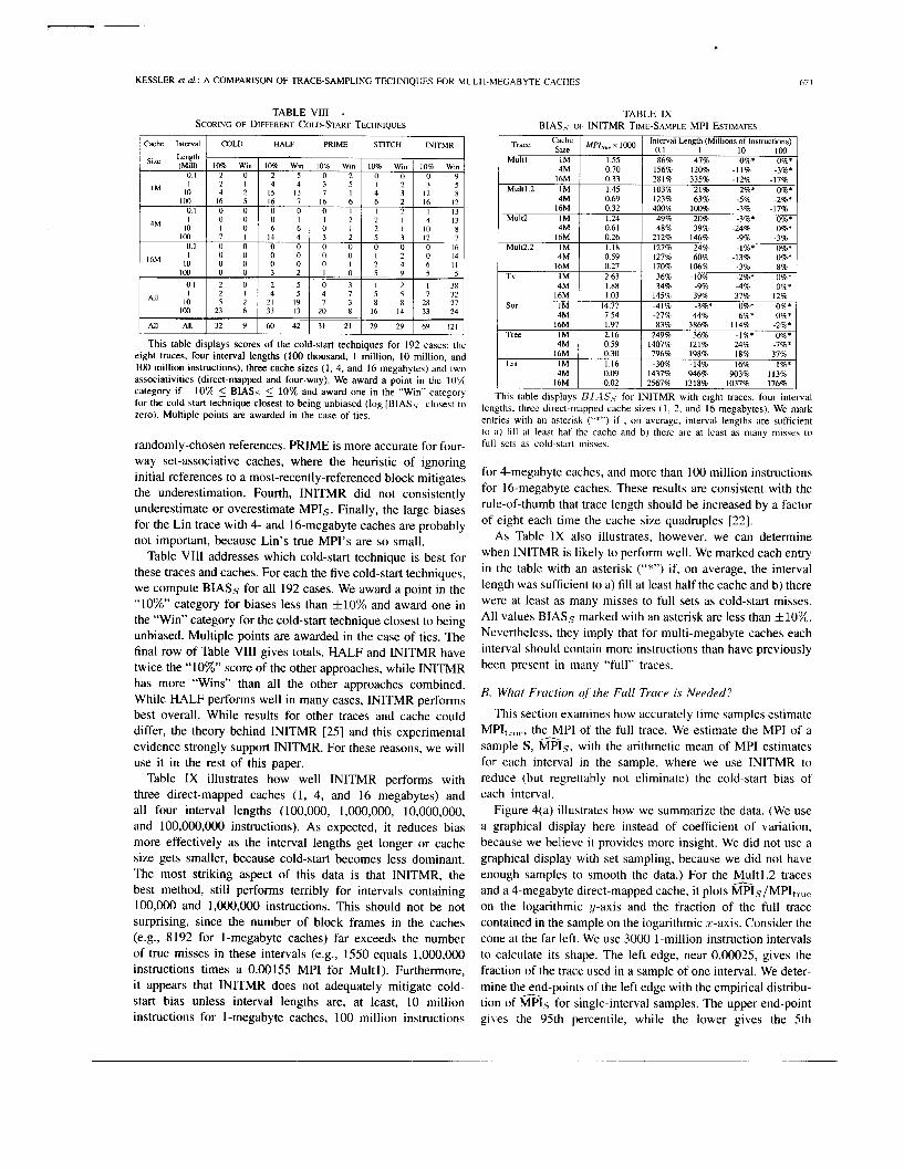
Table VI11 addresses which cold-start technique is best for these traces and caches. For each the five cold-start techniques, we compute BIASs for all 192 cases. We award a point in the “10%” category for biases less than *lo% and award one in the “Win” category for the cold-start technique closest to being unbiased. Multiple points are awarded in the case of ties. The final row of Table VIII gives totals. HALF and INITMR have twice the “10%” score of the other approaches, while INITMR has more “Wins” than all the other approaches combined. While HALF performs well in many cases, INITMR performs best overall. While results for other traces and cache could differ, the theory behind INITMR [25] and this experimental evidence strongly support INITMR. For these reasons, we will use it in the rest of this paper.

Table IX illustrates how well INITMR performs with three direct-mapped caches (1, 4, and 16 megabytes) and all four interval lengths ( 100,000, 1,000,000, 10,000,000, and 100,000,000 instructions). As expected, it reduces bias more effectively as the interval lengths get longer or cache size gets smaller, because cold-start becomes less dominant. The most striking aspect of this data is that INITMR, the best method, still performs terribly for intervals containing 100,000 and 1,O00,000 instructions. This should not be not surprising, since the number of block frames in the caches (e.g., 8192 for 1-megabyte caches) far exceeds the number of true misses in these intervals (e.g., 1550 equals 1,000,000 instructions times a 0.00155 MPI for Multl). Furthermore, it appears that INITMR does not adequately mitigate cold- start bias unless interval lengths are, at least, 10 million instructions for 1-megabyte caches, 100 million instructions

0.70 156% 120% -11% -3%*

1.45 103% 21% 2%* 0%’ 0.69 123% 63% -5% -2%* 0.32 400% 100% -3% -17% 1.24 0.6 I

212% 146% -9% -3% 127% 24% - I % * 0%* 1.18

0.59 127% 60% -13% 0%*

281% 335% -12% -17% 0.33

49% 20% -3%’ o w 48% 39% -24% o s *

0.26

0.27 170% 106% -3% 8% 2.63 36% -10% -2%* n%*

14.77 -41% -3%* o%* n%*

2.16 249% 36% -I%* n%*

1.88 34% -9% 4% O%* I .03 145% 39% 37% 12%

7.54 -27% 44% 6%* 0%* I .97 83% 386% 114% -2%*

0.59 1407% 121% 24% -7%* 0.30 796% 198% 18% -37% 1.16 -30% -14% 16% I%* 0.09 1437% 946% 903% I 1 3 1

67 I

1 6 ~ ih 0.1

All I O

TABLE IX BIAS5 OF INITMR TIME-SAMPLE MPI ESTIMATES

o 0 n n o o I 2 0 1 4 o n n n o i 2 4 6

1 0 0 0 0 3 2 1 o s 9 s 5 2 0 2 5 0 3 I 2 I 3 8

I 2 1 4 5 4 7 5 5 7 3 2 5 2 21 19 7 3 8 X 28 27

100 23 6 33 13 20 8 16 14 33 24

16M I no2 I 2567% 1318% 1037% 176% This table display5 B I 4S5 for INITMR with eight traces, four interval

All All

lengths, three direct-mapped cache sizes ( I , 2, and 16 megabytes). We mark entries with an asterisk (“*”) if , on average, interval lengths are sufficient to a) fill at least haf the cache and h) there are at least as many misses to full sets as cold-start misses.

32 9 60 42 31 21 29 29 69 121

for 4-megabyte caches, and more than 100 million instructions for 16-megabyte caches. These results are consistent with the rule-of-thumb that trace length should be increased by a factor of eight each time the cache size quadruples [22].

As Table IX also illustrates, however, we can determine when INITMR is likely to perform well. We marked each entry in the table with an asterisk (“*”) if, on average, the interval length was sufficient to a) fill at least half the cache and b) there were at least as many misses to full sets as cold-start misses. All values BIASs marked with an asterisk are less than *lo%,. Nevertheless, they imply that for multi-megabyte caches each interval should contain more instructions than have previously been present in many “full” traces.

B. What Fraction of the Full Trace is Needed?

This section examines how accurately time samples estimate MPIt,,,,, the MPI of the full trace. We estimate the MPI of a sample S, =IS, with the arithmetic mean of MPI estimates for each interval in the sample, where we use INITMR to reduce (but regrettably not eliminate) the cold-start bias of each interval.

Figure 4(a) illustrates how we summarize the data. (We use a graphical display here instead of coefficient of variation, because we believe it provides more insight. We did not use a graphical display with set sampling, because we did not have enough samples to smooth the data.) For the %It 1.2 traces and a 4-megabyte direct-mapped cache, it plots MPIs/MPIt,,, on the logarithmic y-axis and the fraction of the full trace contained in the sample on the logarithmic x-axis. Consider the cone at the far left. We use 3000 1 -million-instruction intervals to calculate its shape. The left edge, near 0.00025, gives the fraction of the trace used in a sample of one interval. We determine the end-points of the left edge with the empirical distribu- tion of m1.5 for single-interval samples. The upper end-point gi\es the 95th percentile, while the lower gives the 5th

612

b


j 1 , , tZ"_;t":'\ (,,,,, I , , ,J k,,l , , ,,,,,11 , , , , ,,,, j 100 Million Insrmc~ions - 0 0.001 001 01 1 0001 001 01 I

Fmron of Full Trace Data Fraction of Full Trace Data

(a) (b)

Fig. 4. Cones for time sampling with Multl.2. (akones for M Z s . (b) Cones for MPIs (no hat). This figure displays cones for MPIs (left) and MPIs (right) for the Multl.2 trace and a Cmegabyte direct-mapped cache. For an interval * length and sample size (whose product gives the fraction of the trace used) the height of a cone displays the range of the middle 90% of estimates from many samples. Estimates are unbiased only if they are vertically centered on the horizontalline at 1.0. For an interval length of 1 million instructions, for example, all MPIs displayed here are biased (by cold-start bias not removed by INITMR), while all MPIs am unbiased.

percentile. Thus, thekngth of the left edge is the range of the middle 90% of the MPIs's. We compute other vertical slices similarly. A vertical line (not shown) in the same cone at 0.01 (40 x 0.00025), for example, gives the range of the middle 90% of the MPIs's for samples of 40 intervals each. The other two cones are for interval lengths of 10 million instructions (300 intervals) and 100 million instructions (30 intervals). The right graph gives similar data for MPIs. where we calculate the MPI of each interval with its true initial cache state.

A time sample would meet the 10% sampling goal (Defini- tion 1) if (a) the sample's size times the length of each interval were less than 10% of the trace (e.g., to the left of x-axis value 0.1 in Fig. 4(a) and (b) the cone lies between 0.9 and 1.1 (on the y-axis). Unfortunately, none of the three cones for Multl.2 qualify. The cone for 1-million-instruction intervals is narrow enough but biased too far above 1.0, while the cones of 10 million and 100 million instructions are too wide.

We found similar results for the rest of the traces, displayed in Fig. 5(a) and (b) of Appendix c. The cones for the multiprogrammed traces are similar to those of Multl.2, although Mult2 and Mult2.2 have more cold-start bias. The cones for the single applications, Tree, Tv, Sor, and Lin, are more idiosyncratic, reflecting application-specific behavior. The cones of Sor, for example, are skewed by Sor's behavior of alternating between low and high MPI (with a period of around 300 million instructions [4])

Thus, for these traces and caches (and for direct-mapped and four-way, 1- and 16-megabyte caches [ 101 time sampling fails to meet the 10% sampling goal. Furthermore, even if we eliminate cold-start bias, accurate estimates of MPItrue must use hundred of millions of instructions to capture temporal workload variations. With Multl.2 and a 4-megabyte direct- mapped cache, Fig. 4(b) shows that MPIs is within 10% of MPItrue (for 90% of the samples examined) only with samples of 200 intervals of length 1 million instructions, 65 10-million- instruction intervals, or 20 100-million-instruction intervals. (For much smaller caches, Laha et al. found a sample size of

35 intervals to be sufficient [12].) This is roughly a factor of three decrease in sample size as interval length is multiplied by ten.

Finally, we investigate whether the error in @IS can be estimated from information within the sample itself. We calculate 90% confidence intervals with the same methods as were used for set sampling (Appendix B). These methods, however, provided no information on the magnitude of cold- start bias, because they assume a sample is made up of unbiased observations. Since the cold-start bias (that was not removed by INITMR) is significant in many cases, 90% confidence intervals for time samples often do not contain MPItrue 90% of the time.

Confidence intervals did work in a few cases where samples contained 30 or more intervals and interval lengths were long enough to make cold-start bias negligible [lo]. These cases, however, failed to meet the 10% sampling goal because the samples contained much more than 10% of the trace. Confidence intervals also worked for MPIs (whose expected value is MPItrue because it has no cold-start bias), when samples contain at least 30 intervals.

C. Advantages and Disadvantages of Time Sampling

The major advantage of time sampling is that it is the only sampling technique available for caches with timing-dependent behavior (e.g., that prefetch or are lockup-free [ 111) or shared structures across sets (e.g.. write buffers or victim caching [9]). Furthermore, the cold-start techniques for time sampling can be applied to any full-trace simulation, since a "full" trace is just a single, long observation from a system's workload.

However, in these simulations, time sampling fails to meet the 10% sampling goal for multi-megabyte caches, because it needed long intervals to mitigate cold-start bias and many intervals to capture temporal workload variation. For the cold start techniques we examined, set sampling is more effective than time sampling at estimating the MPI's of our traces with multi-megabyte caches.

V. CONCLUSION

A straightforward application of trace-driven simulation to multi-megabyte caches requires very long traces that strain computing resources. Resource demands can be greatly reduced using set sampling or time sampling. Set sampling estimates cache performance using information from a collection of sets, while time sampling uses information from a collection of trace intervals.

This study is the first to apply set sampling and time sampling to multi-megabyte caches, where they are most useful. We use eight billion-reference traces of large workloads that include multiprogramming but not operating system references [4]. Given a trace and cache, we examine how well both techniques predict the misses per instruction (MPI) of the entire trace. We say a sampling method is effective if it meets the 10% sampling goal: a method meets this goal if, at least 90% of the time, it estimates the trace's true misses per instruction with 5 10% relative error using 5 10% of the trace. Like most trace-driven simulation studies, we do not formally address how our traces relate to the population of

hESFLFR Y I < I / A COMPARISON OF TRACE-SAMPLING TECHNIQUES FOR ULLTl \.ltGABYTE CACHFS

INITMR E\limalcs lor Multl INITMR E w n a i e i tor Mull2 - I ' ' " ' J ' ' 1 ' ' """I ' ' ""'3 t ' ' """I ' ' """I ' ' """I ' ' ""7

Fraction olFull Trace Data

INITMR Esttmales tor Mu112.2

Fracuon of Full Trace Dam

INlTMR Eslimates tar Tree

d I'll - I I I I,,,

= 0001 0 0 1 ( 1 1 I Fraction of Full Trace Data Fraction olFull Tracc Data

Fig. Xa). Cones for time sampling with Multl, Mult2, Mult2.2, and Tree. Similar to Fig. 4(a), these figures display cones for &@IS with the Multl, Mult2, Mult2.2, and Tree traces.

all traces. Readers may accept our results (by assuming our traces are representative of their workload) or re-apply our techniques to their traces.

With our traces and caches, we obtained several results for set sampling. First, how we compute MPI is important. We find that it is much less accurate to normalize misses by the instruction fetches to the sampled sets than by the fraction of sampled sets times all instruction fetches. Second, constructing samples from sets that share some common index bit values works well, since such samples can be used to accurately predict the MPI of multiple alternative caches and caches in hierarchies. Third, sets for our multiprogramming traces behave sufficiently close to normal that confidence intervals are meaningful and accurate. Last and most important, for our traces and caches, set sampling meets the 10% sampling goal.

With our traces and caches, results for time sampling include the following. First, INITMR (Wood et d ' s &,lit [25]) was the most effective technique for reducing cold-start bias, although using half the references in a trace interval to (partially) initialize a cache often performed well. Second, interval lengths must be long to mitigate cold-start bias ( I O million instructions for I-megabyte caches, 100 million instructions for 4-megabyte caches, and more than 100 million instructions for 16-megabyte caches). Third and most important, for these traces and caches, time sampling does not meet the 10%) sampling goal: we needed more than 10% of a trace to get (trace) interval lengths that adequately mitigated cold-start bias and have enough intervals in a sample to make accurate predictions.

Thus, we found that for our traces, set sampling is more effective than time sampling for estimating MPI of the

c d - I , 1 1 1 1 1 1 1 1 I 1 1 1 1 1 1 1 l I 1 1 , 1 , 1

= I l I K l l 001 0 1 I Fraction 111 Full Trxe Data

Fig. 5(b). Cones for time sampling%th Tv, Sor, and Lin. Similar to Fig. 4(a), these figures display cones for MPI5 with the Tv, Sor, and Lin traces. Note that Lin uses a different y-axis scale.

multi-megabyte caches. There are situations, however, when set sampling is not applicable, such as for caches that have time-dependent behavior (e.g., prefetching) or structures used by many sets (e.g., write buffers). In these cases, researchers must choose between using an entire trace and using time sampling. Since any trace can be considered a time sample of size one, either approach requires care to reduce the effect of cold-start bias.

APPENDIX A SYSTEMATIC SAMPLES

This appendix introduces systematic samples with a discus- sion derived from Cochran [5 , ch. 81. We use the notation introduced in Section I11 for consistency.

The variance of the mean of a random sample of size 71

from a population of size s is [8, (2.8)]:

1=1

where mpi, is the ith member of the population and MPItrlle is the population mean.

With systematic sampling, a population of size s is systematically divided into k samples of size 71. By definition, the variance of the mean of a systematic sample, an unbiased estimate of MPItrue, is 18, p. 2081:

where is the mean of the j th systematic sample.

614

TABLE X SET SAMPLING PRECISION FOR 2-wAV

111 6 of Sets 1/64 of Sets Trace Size M ' ' L x 1 ~ cv cv IM 1.19 16/16 2.2% N/A NIA

Multl 4M 0.55 16/16 1.7% 64/64 3.0% 16M 0.26 16/16 1.6% 64/64 2.3% IM 1.18 16/16 1.6% N/A NIA

Multl.2 4M 0.56 16/16 1.2% 64/64 2.2% 16M 0.28 16/16 1.3% 64/64 2.1%

Mult2 4M 0.52 16/16 1.2% 64/64 2.0% 16M 0.24 16/16 1.9% 64/64 3.3% IM 0.98 16/16 1.8% N/A NIA

Mul12.2 4M 0.51 16/16 1.5% 64/64 1.9% 16M 0.22 16/16 2.1% 64/64 3.5% IM 2.31 16/16 0.6% NIA N/A

Tv 4M 1.76 16/16 0.3% 64/64 1.6% 16M 0.98 16/16 0.7% 64/64 1.9% IM 14.66 16/16 0.3% N/A NIA

Sor 4M 7.76 16/16 0.2% 64/64 0.5% 16M 1.92 16/16 0.0% 64/64 0.1%

Tnx 4M 0.49 16/16 1.5% 64/64 3.8% 16M 0.26 16/16 0.4% 64/64 1.1%

IM I .01 16/16 1.9% N/A N/A

IM 1.81 16/16 3.7% NIA N/A

IM 1.10 16/16 2.6% NIA N/A Lin 4M 0.06 16/16 6.0% 44/64 9.8%t

16M 0.02 16/16 0.3% 64/64 0.5%

This table shows the MPI of the full trace for two-way set-associative caches, the fraction of set samples with less than or equal to f10X relative error and the coefficient of variation of the set-sampling MPI estimates, similar to Table IV. Except where marked with a dagger(t), at least 90'A of the samples have relative errors of less than or equal to 610%.

TABLE XI BIAS OF COLD-START TECHNIQUES WITH FOUR-WAY SET-ASSOCIATIVITY

Trace "2: I MPlSx IWO I COLD HALF PRIME STITCH INITMR 1 -.- IM 0.94 +2l% -5% -6% +36% - 1 1 %

Multl 4M 0.44 +106% +29% -51% +80% -4% 16M 0.22 +3l3% +I579 -99% +I678 -81 IM I .20 +15% -5% -9% 6% -7%

Multl.2 4M 0.60 + E l % +21% -40% +43% +I% 16M 0.32 +232% +I186 -57% +IM% -3% IM 0.92 +I496 -5% -18% +33% -16%

Mull2 4M 0.49 +84% +34% -64% +68% +2% 16M 0.22 +3l6% +202% -78% +170% -9% IM 0.96 +16% +IO% -14% +38% -10%

MuIt2.2 4M 0.52 +84% +54% -52% +73% - 1 % 16M 0.25 +285% +221% 415% -161% -14% IM 2.14 +4% -2% -22% +32% -2%

Tv 4M I .53 +14% +6% +I2% +39% -8% I6M 0.82 +99% +75% +195% +87% +32% IM 15.46 +o% -0% +o% - I 1 % -0%

Sor 4M 8.57 +9% - 1 % -12% -8% -2% -. 16M 2 I7 +I585 +34% -81% -4% +60% IM 160 + 1 1 % -3% -9% +35% -6%

Tree 4M 041 +I244 -5% -32% +70% +18% 16M 025 +263% +38% +83% +77% -17% IM 069 +26% +6% +9% +6% +21%

Lin 4M 002 +2763% +I3225 +SI% +778% +I7975 16M 001 +4648% +2248% ---I +873% +I0378

This table displays BZ.4.95 for five cold-start techniques, eight traces, an interval length of I O million instructions, and three four-way set-associative cache sizes ( I , 4, and 16 megabytes).

Since the sample mean for both random and systematic samples are unbiased estimates of the population mean, a sampling method yields a more accurate estimate of the population mean, if and only if the variance of its estimate is less than the variance of the alternative.

Thus, systematic samples obtained by the constant bits method yield more accurate estimates of MPItruc than random samples whenever (Al ) divided by ( A 2 ) is greater than one. Empirical results displayed in Table 111 of Section III-A- 2 show that the ratio is usually greater than one, implying that constant bits samples are generally better than random samples.

We can get more intuition into why systematic samples might be better than random samples by examining the deriva-

. IEEE TRANSACTIONS ON COMPUTERS. VOL. 43. NO. 6. JUNE 1994

tion in [8, p. 2081. Using classical analysis of variance, he shows systematic sampling is more precise, if and only i f

1. n

i = l

where mpi,, is the ith member of the j t h systematic sample. In other words, systematic sampling more precisely estimates the mean of a population if the variance between observations within a systematic sample is greater than the population variance. Thus, we found that systematic samples obtained using constant bits were better than random samples, because systematically sampling sets captured more variation than was present in the population of all sets.

APPENDIX B COMPUTING CONFIDENCE INTERVALS

In this appendix, we describe how we calculate the 90% confidence interval for a sample S containing 71. MPI observations, mpi,, . . . , mpi,,. Since computing confidence intervals for systematic samples is complex [8, Section 8.1 I ] , we compute our confidence intervals by treating our systematic samples as random samples. Because our systematic samples estimate MPItrue with less variance than do random samples (Table 111) the confidence intervals we calculate will tend be larger than necessary. Thus, if sample means are approximately normal, as they are for five of our eight traces (Section III-A- 2), MPItrue should lie within the 90%) confidence intervals of more than 90% of the samples.

We first compute the MPI of sample S , ~ @ I S with:

- 1 M P I ~ = - mpi,,

71, i = l

and estimate MPIs's standard deviation with:

x -L x J-- s - 71,

J;; STDs is the product of three factors: 1 ) the sample standard

deviation of the mpi,'s, given that their true mean is unknown, 2) a 1 adjustment because *Is is the mean of the 71, mpi, 's, and 3) a finite population correction factor [8, (2 .12) ] , which is important only when 76, the sample size, is a substantial fraction of s , the population size. The 90% confidence interval for &@IS is =IS f SFDs . t:'!:, where tE(!< is the value of the student-t statistic that has a tail of 5% (on each end) for 71 - 1 degrees of freedom. We approximate the t-statistic with a normal for most our results, because 71, is large [8, p. 271.

J;;

APPENDIX C ADDITIONAL DATA

In this appendix, we provide additional data to support the claims made in the body of the text. Figures 5(a) and (b) and

KESSLER ef d.: A COMPARISON OF TRACE-SAXIPLISG TECHNIQUES FOR MULTI-MEGABYTE CACHES 675

Tables X and XI are more fully described in the body, where they are referenced.

ACKNOWLEDGMENT

We would like to thank The Western Research Laboratory of Digital Equipment Corporation, especially A. Borg and D. Wall, for the traces used in this study. J . Bartlett, R. De Leone, J . Dion, N. Jouppi, B. Mayo, and D. Stark all were a tremendous help in providing traceable applications. P. Vixie and C. Hawk helped to store the traces. P. Beebe and the Systems Lab were able to satisfy our enormous computing needs. M. Litzkow and M. Livny adapted Condor to the requirements of these simulations. H. Stone gave comments on an earlier version of this work, while S. Adve, V. Adve, G . Gibson and the anonymous referees scrutinized drafts of

paper.

REFERENCES

A. Agarwal, J . Hennessy, and M. Horowitz, “Cache performance of operating system and multiprogramming workloads,” ACM Trans. Computer Syst., vol. 6, no. 4, pp. 393431, Nov. 1988. A. Agarwal and M. Huffman, “Blocking: Exploiting spatial locality for trace compaction,” Proc. Con$ Measurement and Modeling of Computer systems 1990, pp. 48-57. A. Borg, R. E. Kessler, G. Lazana and D. W. Wall, “Long address traces from risc machines: Generation and analysis,” Res. Rep. 89/14, Western Res. Lab., Digital Equipment Corp., Palo Alto, CA, Sept. 1989. A. Borg, R. E. Kessler. and D. W. Wall, “Generation and analysis of very long address traces,” in Proc. 17th Annu. Int. Symp. Comput. Architecture, 1990, pp. 270-279. W. G . Cochran, Sampling Techniques, 3rd ed. New York: John Wiley, 1977. M. C. Easton and R. Fagin, “Cold-start vs. warm-start miss ratios,” Commun. ACM, vol. 21, no. IO, pp. 866-872, Oct. 1978. P. Heidelberger and H. S. Stone, “Parallel trace-driven cache simulation by time partitioning,” IBM Res. Rep. RC 15500, no. 68960, Feb. 1990. M. D. Hill and A. J . Smith, “Evaluating associativity in CPU caches,” IEEE Trans. Comput., vol. 38, no. 12, pp. 16 12- 1630, Dec. 1989. N. P. Jouppi, “Improving direct-mapped cache performance by the addition of a small fully-associative cache and prefetch buffers,’’ in Proc. 17th Annu. Int. Symp. Comput. Architecture, 1990, pp. 364-373. R. E. Kessler, “Analysis of multi-megabyte secondary CPU cache memories,” Ph.D. thesis, Comput. Sci. Tech. Rep. no. 1032, Univ. of Wisconsin-Madison, WI, July 1991. D. Kroft, “Lockup-free instruction fetch/prefetch cache organization,” in Proc. 8th Annu. Int. Symp. Comput. Architecture, 1981, pp. 81-87. S . Laha, J . H. Patel, and R. K. Iyer, “Accurate low-cost methods for performance evaluation of cache memory systems,” IEEE Trans. Comput., vol. 37, no. I I , pp. 1325-1336, Nov. 1988. S . Laha, “Accurate low-cost methods for performance evaluation of cache memory systems,’’ Ph.D. Thesis, Univ. of Illinois Urbana- Champaign, IL, 1988. 1. Miller, J . E. Freund, and R. Johnson, Probability and Staristics for Engineers, fourth ed. M. J . K. Nielsen, “Titan system manual,’’ Res. Rep. 86/1, Western Res. Lab., Digital Equipment Corp., Palo Alto, CA, Sept. 1986. S. A. Przybylski, “Performance-directed memory hierarchy design,” Ph.D. thesis, Tech. Rep. CSL-TR-88-366, Stanford Univ., Stanford, CA, Sept. 1988. S . Przybylski, M. Horowitz, and J . Hennessy, “Characteristics of performance-optimal multi-level cache hierarchies,” in Proc. 16th Annu. Int. Symp. Comput. Architecture. 1989, pp. I 14- I2 1 T. R. Puzak, “Analysis of cache replacement algorithms,” Ph.D. thesis, Univ. of Massachusetts, Amherst. MA, Feb. 1985. A. D. Samples, “Mache: No-loss trace compaction,” in Proc. Int. Conf: Measurement and Modeling of Comput. Sur . , 1989, pp. 89-97. A. J . Smith, “Two methods for the efficient analysis of memory address trace data,” IEEE Trans. Sofncore En?.. vol. SE-3, no. I , pp. Y4-101, Jan. 1977.

Englewood Cliffs, NJ: Prentice Hall, 1990.

121) -, “Cache memories,” Computing Surveys, vol. 14, no. 3 , pp. 473-530, Sept. 1982.

1221 H. S . Stone. High-Performunce Computer Architecture, second ed. Reading, MA: Addison-Wesley, 1990.

[ 2 3 ] W. Wang and J . Baer, “Efficient trace-driven simulation methods for cache performance analysis,” in Proc. Con$ Measurement nnd Modeling of Comput. Sw.. 1990, pp. 27-36.

1241 D. A. Wood, ”The design and evaluation of in-cache address transla- tion,” Ph.D. thesis, Comput. Sci. Division, Tech, Rep, UCBKSD 90/565. Univ. of California, Berkeley, CA, Mar. 1990.

1251 D. A. Wood, M . D. Hill, and R. E. Kessler, “A model for estimating trace-sample miss ratios,” in Proc. ACM SICMETRICS Con$ Meusrrre- ment and Modeling of’ Comput. S.ysr., 199 I , pp. 79-89.

Richard E. Kessler (S’85-M’91) earned the B.S. degree with high distinction in electrical and computer engineering from the University of Iowa, Iowa City, in 1987, and the M.S. and Ph.D. degrees in Computer Science from the University of Wiscon- sin, Madison, in 1989 and 1991, respectively.

He is currently a Senior Architecture Engineer at Cray Research, Inc., Chippewa Falls, WI, special- izing on the Massively-Parallel Processing (MPP) systems. His research interests include the architecture, operating systems, and performance analysis

of computing systems. His recent research focuses largely on the architecture, analysis, and design of large-scale multiprocessing systems.

Dr. Kessler is a member of ACM.

Mark D. Hill (S’81-M’87) earned the B.S.E. degree in computer engineering from the University of Michigan, Ann Arbor, in 1981, and the M.S. and Ph.D. degrees in computer science from the Uni- versity of California, Berkeley, in 1983 and 1987, respectively.

He is currently an Assistant Professor in the Computer Sciences Department at the University of Wisconsin, Madison. He is interested in the design and evaluation of computer architectures. His recent work focuses on the memory systems of high-

performance uniprocessors and shared-memory multiprocessors. J. R. L a m , D. A. Wood and he currently co-lead the ARPA-and NSF-sponsored Wisconsin Wind Tunnel Project that is exploring cost-effective and scalable support for shared memory in parallel supercomputers.

Dr. Hill is a 1989 recipient of the National Science Foundation’s Presiden- tial Young Investigator award and a member of ACM.

David A. Wood (S’81-M’90) received the B.S. degree in electrical engineering and computer science at the University of California, Berkeley, in I98 I . After graduation, he worked on one of the earli- est shared-memory multiprocessors at the Synapse Computer Corporation, where he helped develop a relational database system. He then returned to U.C. Berkeley, where he earned the Ph.D. degree in computer science in 1990 under Prof. R. Katz.

He is currently an Assistant Professor in the Computer Sciences and Electrical and Computer

Engineering Departments at the University of Wisconsin, Madison. His interests range from VLSI design to operating systems, but focus on the design and evaluation of computer architectures, with an emphasis on memory systems for shared-memory multiprocessors. Together with M. D. Hill and J . R. Larus, he co-leads the NSF-sponsored Wisconsin Wind Tunnel Project that is exploring cost-effective and scalable support for shared memory in parallel supercomputers.

Dr. Wood i \ a 1991 recipient of the National Science Foundation‘s Presidential Young Investigator award and a member of the ACM.

Documents

A comparison of trace-sampling techniques for multi