Embed Size (px)
Citation preview

Caroline BAYR, Bakk.techn.
A comparison of the Markowitzportfolio optimization with some
robust counterparts
MASTERARBEIT
zur Erlangung des akademischen Grades einer Diplom-Ingenieurin
Masterstudium Finanz- und Versicherungsmathematik
Technische Universitat Graz
Betreuerin:Ao. Univ.-Prof. Dipl.-Ing. Dr.techn. Eranda DRAGOTI-CELA
Institut fur Optimierung und Diskrete Mathematik (Math B)
Graz, im Mai 2010

Statutory Declaration
I declare that I have authored this thesis independently, that I have not used other thanthe declared sources/resources, and that I have explicitely marked all material whichhas been quotes either literally or by content from the used sources.
. . . . . . . . . . . . . . . . . . . . . . . . . . . . . . . . . .date
. . . . . . . . . . . . . . . . . . . . . . . . . . . . . . . . . . . . . . . . . . .(signature)

Preface
This master thesis is about portfolio optimization considering uncertain input parame-ters.
In the first chapter, we introduce the classical mean-variance optimization model ofHarry Markowitz. We assume that the expected returns and the covariance matrix,which is used as risk measure, are known. Some related portfolio optimization problemsand the corresponding solution methods are discussed.
In the second chapter we define robust optimization in general and describe differentproblems: uncertainty in the objective function, uncertainty in the constraints and theconcept of relative robustness. Further we discuss some strategies like resampling ofdata and solution methods for conic optimization problems needed when dealing withrobust optimization problems.
The robust portfolio optimization is considered in the third chapter. There we assume,that the knowledge about expected returns and the covariance matrix is uncertain; forthese inputs we only have estimations leading to uncertain input data. We include thesedata in the optimization problem by assuming that they lie in so-called uncertainty sets.The resulting optimization problems are formulated and solved.
In the last chapter, the models described in the previous chapters of the thesis are ap-plied to an instance of a portfolio optimization problem focussing on the comparison ofclassical optimization models with their robust counterparts.
I want to thank Ao. Univ.-Prof. Dipl.Ing Dr.techn. Eranda Dragoti-Cela for the faith-ful supervision, the patience and the helpful advices. I also want to thank all people,who helped me with this master thesis, especially my parents for supporting me dur-ing my study time and my boyfriend Andreas Angermann for his motivation all the time.
All errors are my own.
Graz, May 2010 Caroline Bayr

Contents
1 Markowitz: Classical Mean-Variance Optimization 11.1 Introduction . . . . . . . . . . . . . . . . . . . . . . . . . . . . . . . . . . . 11.2 Single-period mean-variance model . . . . . . . . . . . . . . . . . . . . . . 2
1.2.1 Risky assets . . . . . . . . . . . . . . . . . . . . . . . . . . . . . . . 61.2.2 Risky assets and riskless cash . . . . . . . . . . . . . . . . . . . . . 121.2.3 Risky assets, riskless cash and guaranteed total loss . . . . . . . . 171.2.4 The influence of inequalities . . . . . . . . . . . . . . . . . . . . . . 201.2.5 Critical line algorithm . . . . . . . . . . . . . . . . . . . . . . . . . 211.2.6 Downside risk . . . . . . . . . . . . . . . . . . . . . . . . . . . . . . 24
1.3 Multi-period mean-variance model . . . . . . . . . . . . . . . . . . . . . . 271.4 Conclusion . . . . . . . . . . . . . . . . . . . . . . . . . . . . . . . . . . . 30
2 Robust Optimization 322.1 Introduction . . . . . . . . . . . . . . . . . . . . . . . . . . . . . . . . . . . 322.2 Uncertainty sets . . . . . . . . . . . . . . . . . . . . . . . . . . . . . . . . 332.3 Models of robustness . . . . . . . . . . . . . . . . . . . . . . . . . . . . . . 35
2.3.1 Constraint robustness . . . . . . . . . . . . . . . . . . . . . . . . . 352.3.2 Objective robustness . . . . . . . . . . . . . . . . . . . . . . . . . . 362.3.3 Relative robustness . . . . . . . . . . . . . . . . . . . . . . . . . . . 402.3.4 Adjustable robust optimization . . . . . . . . . . . . . . . . . . . . 41
2.4 Strategies . . . . . . . . . . . . . . . . . . . . . . . . . . . . . . . . . . . . 422.4.1 Sampling . . . . . . . . . . . . . . . . . . . . . . . . . . . . . . . . 432.4.2 Conic optimization . . . . . . . . . . . . . . . . . . . . . . . . . . . 43
2.5 Conclusion . . . . . . . . . . . . . . . . . . . . . . . . . . . . . . . . . . . 46
3 Robust portfolio optimization 473.1 Portfolio resampling technique . . . . . . . . . . . . . . . . . . . . . . . . 473.2 Robust portfolio allocation . . . . . . . . . . . . . . . . . . . . . . . . . . 49
3.2.1 Uncertainty in the expected returns . . . . . . . . . . . . . . . . . 493.2.2 Uncertainty in covariance matrix of returns . . . . . . . . . . . . . 52
3.3 Relative robustness . . . . . . . . . . . . . . . . . . . . . . . . . . . . . . . 573.4 Multi-period robustness . . . . . . . . . . . . . . . . . . . . . . . . . . . . 613.5 Conclusion . . . . . . . . . . . . . . . . . . . . . . . . . . . . . . . . . . . 65

4 Portfolio Optimization in Practice 664.1 Data . . . . . . . . . . . . . . . . . . . . . . . . . . . . . . . . . . . . . . . 66
4.1.1 Implementation in R . . . . . . . . . . . . . . . . . . . . . . . . . . 664.1.2 Data Analysis . . . . . . . . . . . . . . . . . . . . . . . . . . . . . . 71
4.2 Comparison of the parameters . . . . . . . . . . . . . . . . . . . . . . . . . 754.2.1 Implementation in MATLAB . . . . . . . . . . . . . . . . . . . . . 80
4.3 Comparison: Classical optimization problems with the robust counterparts 814.3.1 Uncertainty in the expected returns . . . . . . . . . . . . . . . . . 814.3.2 Uncertainty in the expected returns and the covariance matrix:
Simple case . . . . . . . . . . . . . . . . . . . . . . . . . . . . . . . 854.3.3 Uncertainty in the expected returns and the covariance matrix:
General case . . . . . . . . . . . . . . . . . . . . . . . . . . . . . . 894.3.4 Stability of the optimization problems . . . . . . . . . . . . . . . . 92
4.4 Conclusion . . . . . . . . . . . . . . . . . . . . . . . . . . . . . . . . . . . 94

1 Markowitz: Classical Mean-VarianceOptimization
1.1 Introduction
This chapter is based on the paper of Steinbach [1] and the paper of A. and D. Nieder-mayer [2]. The duality theory is from the script of Burkard [3] and the book of Fabozziet al. [5], Chapter 9.
In this chapter we discuss the classical portfolio optimization by Harry Markowitz, theso-called mean-variance optimization. Markowitz proposed an optimization model to geta high reward with low risk. This model is sufficiently simple to be solved numericallyand can be used in practice.First of all we will analyze the single-period mean-variance model. There we show theoptimization problem for several assumptions: First we discuss the problem with riskyassets only. Then we include the possibility to invest in riskless cash and the third stepis to look at the optimization of investing in an account with guaranteed total loss.We will also consider the influence of constraints with inequalities instead of equations.Since the choice of the risk measure influences the solutions of an optimization problem,we want to discuss the downside risk optimization too where we use the semi-varianceinstead of the variance as risk measure. We need some certain assumptions of the returndistributions.Then we want to consider the multi-period mean-variance model. In this context weneed so-called scenario trees.
Throughout this master thesis we assume that short selling is not allowed.
1

1 Markowitz: Classical Mean-Variance Optimization
1.2 Single-period mean-variance model
In our considerations we can invest in n assets over a certain period of time. A portfolioover these n assets is specified by the so-called portfolio vector w ∈ Rn, where wi isthe percentage of capital invested in asset i. Let us denote the random vector of assetreturns by r ∈ Rn. Denote by pi the price of asset i at time ti and by pi+1 the price ofasset i at time ti+1 for 1 ≤ i ≤ n. Then the return of asset i is given as ri = pi+1−pi
pi. At
the end of the period [ti, ti+1] the portfolio return is given as R =n∑i=1
riwi = r′w, where
r′ denotes the transposed vector of r. Assume that the asset returns have expectationµr := E[r] and covariance matrix
Σ := E[(r − µr)(r − µr)′] = E[rr′]− µrµ′r.
The total return of the portfolio is a random variable which depends on the portfoliovector (wi): R = r′w. The aim is to determine a portfolio vector w which leads to a re-turn distribution fullfilling the investor’s needs. In this context we define two importantquantities, reward and risk, as follows:
Definition 1.1: RewardThe reward of a portfolio is the mean of its return,
µ(w) := E[R] = E[r′w] = µ′rw.
Definition 1.2: RiskThe risk of a portfolio is the variance of its return,
σ2(w) := V ar[R] = E[(r′w − E[r′w])2] = E[w′(r − µr)(r − µr)′w] = w′Σw.
We want to maximize the reward and minimize the risk leading to the optimizationproblem:
maxw
{cµ(w)− 1
2σ2(w)
}(1.1)
s.t. e′w = 1,
wi ≥ 0, ∀i,
2

1 Markowitz: Classical Mean-Variance Optimization
where e ∈ Rn denotes the vector of all ones. The investor tries to get a good trade-offbetween reward and risk. The equation e′w = 1 is called the budget equation and spec-ifies the initial wealth.Problem 1.1 can be reformulated as one of the following two optimization problems,which are dual to each other. For understanding we give a short discussion to duality ofoptimization problems (see Fabozzi et al. [5], Chapter 9).The variables of a dual problem are related to variables of the corresponding primalproblem. If the primal optimization problem is a maximization then the dual optimiza-tion problem is a minimization and conversely, if the primal problem is minimizationthen the dual problem will be maximization. The number of variables of the primalproblem is equal to the number of constraints of the dual problem and vice versa. Thereare several advantages of dual optimization problems:
• The dual problem is often better tractable from a theoretical or computationalpoint of view. This can be used to compute the primal and dual solutions.
• If we have a convex optimization problem, then we can solve the dual problem andthe objective value is the same as in the primal problem.
So we use dual problems, because they are often easier to solve than the primal problems.
Dual optimization problems also play a major part in formulations of robust optimizationproblems, which are discussed in the following chapters. Now we want to summarizebriefly how to obtain the dual of a problem given.Consider the following primal optimization problem:
minxf(x) (1.2)
s.t. gi(x) ≤ 0, i = 1, . . . , n.
First we formulate the Lagrangian to put the constraints of the primal problem in theobjective function for which we use n nonnegative multipliers ui:
L(x, u) = f(x)− u′g(x).
Now we construct the dual function:
L∗(u) = minx
{f(x) + u′g(x)
}.
Finally we can formulate the dual optimization problem:
maxu
L∗(u) (1.3)
s.t. u ≥ 0.
3

1 Markowitz: Classical Mean-Variance Optimization
In the following passage we review some basics of duality theory in linear and quadraticoptimization. First consider linear optimization problems:
• Primal problem:maxx
c′x (1.4)
s.t. Ax ≤ b,x ≥ 0.
• Dual problem:minub′u (1.5)
s.t. A′u ≥ c,u ≥ 0.
We can formulate two theorems about the solutions of primal and dual problems:
Theorem 1.1: Weak DualityFor every feasible solution x of the primal problem and every feasible u of the dualproblem holds:
c′x ≤ b′u.
Proof:From A′u ≥ c, x ≥ 0 and Ax ≤ b follows:
c′x ≤ u′Ax ≤ u′b.
�
Theorem 1.2: DualityIf one of two dual linear optimization problems has a finite optimal solution, then theother problem has a finite optimal solution and for the optimal values x∗ and u∗ of theobjective function holds:
c′x∗ = b′u∗.
4

1 Markowitz: Classical Mean-Variance Optimization
For the proof, see Burkard [3], page 87.
Now we consider the duality in quadratic optimization:
• Primal problem:
minx
{1
2x′Qx+ c′x
}(1.6)
s.t. Ax ≥ b.
• Dual problem:
maxu
{u′b− 1
2(c−A′u)′Q−1(c−A′u)
}(1.7)
s.t. u ≥ 0.
Look up the book of Fazozzi et al. [5], Chapter 9.
Now consider the mean-variance optimization Problem 1.1 again. An equivalent formu-lation of Problem 1.1 is the following:
maxw
µ(w) (1.8)
s.t. e′w = 1,
σ2(w) ≤ s.wi ≥ 0, ∀i.
The equivalence of Problem 1.1 and 1.8 will be shown in Section 1.2.1.
In this model we maximize the reward subject to the budget equation and the constraintthat the risk is lower than a fixed level s.
The dual problem is to minimize the risk subject to the budget equation and the con-straint that the reward is fixed at level m.
5

1 Markowitz: Classical Mean-Variance Optimization
minw
1
2σ2(w) (1.9)
s.t. e′w = 1,
µ(w) = m,
wi ≥ 0, ∀i.
Problem 1.8 has a linear objective function and convex quadratic restrictions and Prob-lem 1.9 has a convex quadratic objective function and linear restrictions. The convexityof the quadratic restrictions or the quadratic goal function, follows from the positivesemidefinitness of Σ as a covariance matrix. So numerically Problem 1.9 is easier tosolve than Problem 1.8.
Further in this section the relationship between these optimization problems is discussed.We extend the general single-period model by including riskless cash, guaranteed loss,inequalities and downside risk.
1.2.1 Risky assets
Now consider the simplest situation with a portfolio consisting of n risky assets only.We need two assumptions on the return distribution.
Assumptions:
• (A1) Σ > 0, the covariance matrix is positive definite.:All n assets and any convex combination of them are risky.
• (A2) µr is not a multiple of e: µr 6= ke for k ∈ N:This implies n ≥ 2 and guarantees that the situation does not degenerate. Other-wise the optimal portfolio of Problem 1.1 would always be the same: w = Σ−1e
e′Σ−1eregardless of the trade-off parameter c. Furthermore the constraints of Problem1.9 would be violated except of one specific value of the desired reward, namely
m = µ′ren .
To solve Problem 1.1 we minimize the negative utility function and get the followingoptimization problem:
6

1 Markowitz: Classical Mean-Variance Optimization
minw
{1
2w′Σw − cµ′rw
}(1.10)
s.t. e′w = 1,
wi ≥ 0, ∀i.
The Lagrangian is
L(w, λ; c) =1
2w′Σw − cµ′rw − λ(e′w − 1).
∂L
∂w= w′Σ− cµr − λe = 0. (1.11)
The optimal solution for the portfolio vector w is
w∗ = Σ−1[cµr + λe].
To get the optimal multiplier λ we substitute the optimal w in the budget equation:
e′[Σ−1[cµr + λe]] = 1
λ∗ =1− ce′Σ−1µr
e′Σ−1e. (1.12)
The optimal reward m is obtained by substitution of the optimal w in m = µ′rw:
m∗ = cµ′rΣ−1µr + λe′Σ−1µr =
c(e′Σ−1eµ′rΣ−1µr − [e′Σ−1µr]
2) + e′Σ−1µre′Σ−1e
(1.13)
This solution is unique because the objective is strongly convex and Constraint 1.11 isof full rank.
Thus Problem 1.9 is easier to solve numerically.
7

1 Markowitz: Classical Mean-Variance Optimization
minw
1
2w′Σw (1.14)
s.t. e′w = 1,
µrw = m,
wi ≥ 0, ∀i.
The Lagrangian is
L(w, λ, c;m) =1
2w′Σw − λ(e′w − 1)− c(µrw −m).
∂L
∂w=w′Σ− λe− cµr = 0.
The optimal solution for the portfolio vector w is
w∗ = Σ−1(λe+ cµr).
To get the optimal value c we substitute the optimal value of w in the budget equation:
e′(Σ−1(λe+ cµr)) = 1.
Hence we get λ:
λ =1− e′Σ−1µrc
e′Σ−1e. (1.15)
By substituting the optimal w in the equation m = µ′rw we get
m = µr(Σ−1(λe+ cµr)). (1.16)
In Equation 1.16 we substitute Equation 1.15 for λ and we get the optimal c:
8

1 Markowitz: Classical Mean-Variance Optimization
m =µr(Σ−1((
1− e′Σ−1µrc
e′Σ−1e)e+ cµr)).
m =µ′rΣ
−1e− e′Σ−1µre′Σ−1µrc
e′Σ−1e+ cµ′rΣ
−1µr.
me′Σ−1e− µrΣ−1e =c(−(e′Σ−1µr)2 + µ′rΣ
−1µre′Σ−1e).
c∗ =me′Σ−1e− µrΣ−1e
µ′rΣ−1µre′Σ−1e− (e′Σ−1µr)2
. (1.17)
For the optimal λ we substitute the optimal c from 1.17 in Equation 1.15:
λ =1− e′Σ−1µr(
me′Σ−1e−µrΣ−1eµ′rΣ
−1µre′Σ−1e−(e′Σ−1µr)2)
e′Σ−1e.
λ =µ′rΣ
−1µre′Σ−1e− (e′Σ−1µr)
2 − e′Σ−1µre′Σ−1em+ (e′Σ−1µr)
2
e′Σ−1e(µ′rΣ−1µre′Σ−1e− (e′Σ−1µr)2)
.
λ∗ =µrΣ
−1µr − e′Σ−1µrm
µ′rΣ−1µre′Σ−1e− (e′Σ−1µr)
. (1.18)
Theorem 1.3:Problem 1.10 with parameter c and Problem 1.14 with parameter m are equivalent ifand only if c equals the optimal reward multiplier λ of Problem 1.14, or equivalently, mequals the optimal reward multiplier λ of Problem 1.10.
Proof :The conditions c = e′Σ−1em−e′Σ−1µr
e′Σ−1eµ′rΣ−1µr−[e′Σ−1µr]2
and m = c(e′Σ−1eµ′rΣ−1µr−[e′Σ−1µr]2)+e′Σ−1µr
e′Σ−1e
are equivalent. For the optimal reward multipliers of Problem 1.10 and 1.14 follows thatthey are identical:
9

1 Markowitz: Classical Mean-Variance Optimization
λ1 =1− ce′Σ−1µr
e′Σ−1e
=e′Σ−1eµ′rΣ
−1µr − [e′Σ−1µr]2 − e′Σ−1ee′Σ−1µrm+ [e′Σ−1µr]
2
e′Σ−1ee′Σ−1eµ′rΣ−1µr − [e′Σ−1µr]2
=e′Σ−1eµ′rΣ
−1µr − e′Σ−1ee′Σ−1µrm
e′Σ−1ee′Σ−1eµ′rΣ−1µr − [e′Σ−1µr]2
=µ′rΣ
−1µr − e′Σ−1µrm
e′Σ−1eµ′rΣ−1µr − [e′Σ−1µr]2
= λ2.
So the optimal portfolios are equivalent.
�
To continue we need the following definition of an efficient frontier and a Pareto-optimalsolution.
Definition 1.3: Efficient frontierThe efficient frontier is a curvature containing points (m,σ2) where σ2 is the optimalrisk. For a given level of return all points in this curve correspond to portfolios withlowest risk.
The restrictions of Problem 1.10 are restrictions of Problem 1.14, too. The later problemcontains one more additional restriction, the so-called reward restriction. These n + 2restrictions define for n+ 3 variables w, λ, c,m a one-dimensional affine subspace whichis parametrized by c in Problem 1.10 and by m in Problem 1.14. The optimal risk is aquadratic function of m, σ2(m), which graph is called the efficient frontier.
Definition 1.4: Pareto-optimalityLet X be a feasible set. A solution x∗ ∈ X is called Pareto-optimal, if there exists nox ∈ X : f(x) < f(x∗).
Generally, the efficient frontier refers to the set of all Pareto-optimal solutions of an opti-mization problem. In our considerations it applies to the upper branch corresponding tom ≥ m only, where m is the optimal reward. The lower branch corresponds to m ≤ m.All feasible portfolios are on the right and below the efficient frontier.
10

1 Markowitz: Classical Mean-Variance Optimization
Figure 1.1: Efficient frontier of a portfolio with risky assets
Theorem 1.4:The optimal risk in Problem 1.10 and 1.14 is
σ2(m) =e′Σ−1em2 − 2e′Σ−1µrm+ µ′rΣ
−1µre′Σ−1eµ′rΣ
−1µr − [e′Σ−1µr]2.
It takes the global minimum over all rewards at
m =e′Σ−1µre′Σ−1e
and has the positive value in this case
σ2(m) =1
e′Σ−1e.
The associated solution is
w =Σ−1e
e′Σ−1e, λ =
1
e′Σ−1e, c = 0.
Proof :We use Definition 1.2 of the optimal risk and the solution of Problem 1.14,
11

1 Markowitz: Classical Mean-Variance Optimization
σ2(m) =w′Σw = (λe+ cµr)′Σ−1(λe+ cµr)
=λ2e′Σ−1e+ 2λce′Σ−1µr + c2µrΣ−1µr
=λ(λe′Σ−1e+ ce′Σ−1µr) + c(λe′Σ−1µr + cµrΣ−1µr).
Using the expressions on the right hand sides of Equations 1.12 and 1.13 we get
σ2(m) = λ+ cm.
With Equations 1.17 and 1.18 we get
σ2(m) =e′Σ−1em2 − 2e′Σ−1µrm+ µrΣ
−1µre′Σ−1eµ′rΣ
−1µr − [e′Σ−1µr]2. (1.19)
Differentiating Equation 1.19 with respect to m we obtain
2e′Σ−1em− 2e′Σ−1µr =0
m =e′Σ−1µre′Σ−1e
Substituting this optimal minimum in Equations 1.17 and 1.18 we get the associatedsolution w, λ and c:
w =Σ−1e
e′Σ−1e, λ =
1
e′Σ−1e, c = 0.
�
1.2.2 Risky assets and riskless cash
Consider n risky assets and also a cash account wc with deterministic return rc = E[rc].So the portfolio includes (w,wc) and the variables w, r, µr and Σ belong to the risky part.
Assumptions: We get two similar assumptions as in the previous section, but we replace(A2) by another condition where the portfolio consists just of one risky asset and thecash account.
12

1 Markowitz: Classical Mean-Variance Optimization
• (A1) Σ > 0, the covariance matrix is positive semidefinite.
• (A2) µr 6= rce: No degenerate situations can occur.
We formulate the following optimzation problem
minw,wc
1
2
(wwc
)′(Σ 00 0
)(wwc
)=
1
2w′Σw (1.20)
s.t. e′w + wc = 1,
µ′rw + rcwc = m,
wc ≥ 0, wi ≥ 0, ∀i.
The Lagrangian is
L(w,wc, λ, c;m) =1
2w′Σw − λ(e′w + wc − 1)− c(µ′rw + rcwc −m). (1.21)
By differentiating the Lagrangian 1.21 with respect to w we get
w′Σ− λe− cµr = 0
w = Σ−1(λe+ cµr). (1.22)
By differentiating the Lagrangian 1.21 with respect to wc we get
−λ− crc = 0
λ = −crc. (1.23)
Putting Equation 1.23 in Equation 1.22 we get the optimal solution for w
w∗ = cΣ−1(µr − rce). (1.24)
By using the budget equation and substituting the optimal w from Equation 1.24 in thebudget equation we get
wc = 1− c(e′Σ−1µr − rce′Σ−1e). (1.25)
13

1 Markowitz: Classical Mean-Variance Optimization
By putting Equations 1.24 and 1.25 on the left hand side of the second restriction ofProblem 1.20 we get the optimal c
c∗ =m− rc
(µr − rce)′Σ−1(µr − rce). (1.26)
The optimal risk occurs to using the definition of risk σ2(m) = w′Σw and Equations1.24 and 1.26:
σ2(m) =(m− rc)2
(µr − rce)′Σ−1(µr − rce).
Differentiating with respect to m we get
2(m− rc) = 0
and therefore the global minimum is taken at m = rc with σ2(m) = 0. The associatedsolution is to invest 100% of the capital in cash and the risk vanishes: (w,wc) = (0, 1)and λ = c = 0.
The trade-off version of Problem 1.20 is
minw,wc
{1
2w′Σw − c(µ′rw + rcwc)
}(1.27)
s.t. e′w + wc = 1,
wc ≥ 0, wi ≥ 0, ∀i.
Theorem 1.5:Problem 1.20 with parameter m and Problem 1.27 with parameter c are equivalent ifand only if m = rc + c(µr − rce)′Σ−1(µr − rce).
Proof :Analogous to the proof of Theorem 1.3.
�
14

1 Markowitz: Classical Mean-Variance Optimization
For m = rc the whole capital is invested in cash. Otherwise e′w = c(e′Σ−1µr−rce′Σ−1e)is invested in risky assets, so the risk is positive because the optimal portfolio is a mix-ture of the risky portfolio (Σ−1(µr − rce), 0) and cash (0, 1).
The following theorem shows, how the risk reduces, if we have a portfolio with cashadded.
Theorem 1.6:The risk in Problem 1.20 with cash is lower than in Problem 1.14 without cash as soonas the portfolio invests in risky assets.If e′Σ−1µr 6= rce′Σ−1e: The efficient frontiers touch in the point
m = rc +(µr − rce)′Σ−1(µr − rce)e′Σ−1µr − rce′Σ−1e
,
σ2(m) =(µr − rce)′Σ−1(µr − rce)(e′Σ−1µr − rce′Σ−1e)2
.
If w is an optimal solution of Problem 1.14, then is (w, 0) an optimal solution of Problem1.20. Vice-versa, the optimal solution of Problem 1.20 has the form (w, 0) and w is thenan optimal solution of Problem 1.14.If e′Σ−1µr = rce′Σ−1e: wc = 1, e′w = 0 and risks differ by 1
e′Σ−1e:
(m− rc)2
(µr − rce)′Σ−1(µr − rce)+
1
e′Σ−1e=e′Σ−1em2 − 2e′Σ−1µrm+ µ′rΣ
−1µre′Σ−1eµ′rΣ
−1µr − [e′Σ−1µr]2.
Proof :If e′Σ−1µr 6= rce′Σ−1e: The solution of Problem 1.20 is wc = 0 because we do not investin cash with
c =1
e′Σ−1µr − rce′Σ−1e, λ = − rc
e′Σ−1µr − rce′Σ−1e.
This results in the values of m and σ2(m) by substituting it in m = rc + c(µr −rce)′Σ−1(µr − rce) and σ2(m) = (m−rc)2
(µr−rce)′Σ−1(µr−rce) . If m is substituted in the solu-
tions of Problem 1.14 for λ and c, the values of both problems will be the same. So theportfolios are equivalent. To get the curvatures of the efficient frontiers we derive both
risks twice and get for Problem 1.14 ∂2σ2(m)∂m2 = 2e′Σ−1e
e′Σ−1eµ′rΣ−1µr−[e′Σ−1µr]2
and for Problem
1.20 ∂2σ2(m)∂m2 = 1
(µr−rce)′Σ−1(µr−rce) . We compare these values and get
2e′Σ−1e
e′Σ−1eµ′rΣ−1µr − [e′Σ−1µr]2
− 1
(µr − rce)′Σ−1(µr − rce)> 0.
15

1 Markowitz: Classical Mean-Variance Optimization
Therefore the risk of Problem 1.20 is lower than in Problem 1.14 if wc 6= 0.
If e′Σ−1µr 6= rce′Σ−1e: The efficient frontiers of Problems 1.14 and 1.20 touch in m = rc
and they have identical curvatures.
�
Figure 1.2: Capital market line with the (m,σ2) combination M
In Figure 1.2 we see the capital market line, which corresponds to linear combinationsof the riskless portfolio A and the risky portfolio M. In point M, no capital is investedin cash, so we have wc = 0. The portfolio corresponding to M is called market portfolio.In the point A there is m = rc, so nothing is invested in risky assets and wc = 1.
The following Lemma shows, that it does not make sense to have more than one risklessasset.
Lemma 1.1: (Arbitrage)Any portfolio with two or more riskless assets can realize any desired reward with zerorisk.
16

1 Markowitz: Classical Mean-Variance Optimization
Proof :Consider two riskless assets with different returns rc and rd. For every desired return mwe choose the weights
wc =m− rd
rc − rd, wd = 1− wc,
and invest nothing in other assets. The expected return of this portfolio is m and itsvariance is equal to 0.
wcrc + wdrd =m− rd
rc − rdrc + (1− wc)rd =
mrc − rdrc + rcrd − (rd)2 −mrd + (rd)2
rc − rd= m
�
1.2.3 Risky assets, riskless cash and guaranteed total loss
Consider again a portfolio with n risky assets, a riskless cash account, but include alsoan ”asset” wl with guaranteed total loss and rl = E[rl] = 0. First it seems to be senselessto invest in an asset with guaranteed loss, but we will see, that it makes sense.
Assumptions: We have the same assumptions (A1) and (A2) as before but also a thirdone: we require positive cash return. We also assume that the reward of wl is equal to0.
• (A1) Σ > 0, the covariance matrix of risky assets is positive definite.
• (A2) µr 6= rce.
• (A3) rc > 0 (and rc > rl is reasonable.)
We formulate the following optimization problem
minw,wc,wl
1
2
wwc
wl
′Σ 0 00 0 00 0 0
wwc
wl
=1
2w′Σw (1.28)
s.t. e′w + wc + wl = 1,
µ′rw + rcwc = m,
wc ≥ 0, wl ≥ 0, wi ≥ 0, ∀i.
17

1 Markowitz: Classical Mean-Variance Optimization
The Lagrangian is
L(w,wc, wl, λ, c, η;m) =1
2w′Σw−λ(e′w+wc +wl− 1)− c(µ′rw+ rcwc−m)− η(wl− 0).
(1.29)
By differentiating the Lagrangian we get the optimal solutions according to the followingtheorem.
Theorem 1.7:Problem 1.28 has unique solutions w,wc, wl, λ, c, η, where η is the multiplier of theconstraint wl ≥ 0.
• For m > rc: The solution is identical to the solution of Problem 1.20. We havewl = 0 and η = −λ > 0.
• For m ≤ rc: The optimal solution is to invest in a linear combination of the tworiskless assets:
w = 0, wc =m
rc, wl = 1− m
rc, λ = c = η = 0.
Proof:We differentiate the Lagrangian 1.29 with respect to w and wc and obtain Equations 1.22and 1.23. If we differentiate the Lagrangian with respect to wl we obtain the additionalequation
η = −λ.
If m > rc:Then c > 0, which leads to λ > 0 and −η > 0. With the restriction wlη = 0 followswl = 0 and we obtain Problem 1.20.
If m ≤ rc:Then c = 0 which leads to λ = −η = 0 and w = 0.From the budget equation we get with w = 0: wc + wl = 1 and it follows wl = 1− wc.From the reward equation we get with w = 0: rcwc = m and it follows wc = m
rc andwl = 1− m
rc .
�
The trade-off version of Problem 1.28 is
18

1 Markowitz: Classical Mean-Variance Optimization
minw,wc,wl
{1
2w′Σw − c(µrw + rcwc)
}(1.30)
s.t. e′w + wc + wl = 1,
wc ≥ 0, wl ≥ 0, wi ≥ 0, ∀i.
Theorem 1.8:Problem 1.30 with c > 0 and Problem 1.28 with m > rc are equivalent if and only ifm = rc + c(µr − rce)′Σ−1(µr − rce).Problem 1.30 with c = 0 has the same solutions as Problem 1.28 with m ≤ rc.Problem 1.30 with c < 0 is unbounded and has no solution.
Proof:The restrictions of both problems are nearly the same, only the reward condition inProblem 1.28 is included. The Lagrangian of Problem 1.30 is
L(w,wc, wl, λ, c, η;m) =1
2w′Σw − c(µ′rw + rcwc)− λ(e′w + wc + wl − 1)− η(wl − 0).
Differentiating according to wc we get
−crc = λ. (1.31)
By differentiating with respect to wl we get
η = −λ. (1.32)
Putting Equation 1.31 in Equation 1.32 we get η = rcc.If c > 0: η > 0 and m > rc. If c = 0: η = 0 and m ≤ rc. If c < 0: η < 0 and thereProblem 1.30 has no solution. For these results see Theorem 1.5 where the equationm = rc + c(µr − rce)′Σ−1(µr − rce) holds.
�
At the beginning of this section we pointed out, that it is strange to invest in an assetwith guaranteed loss. But why does it make sense?The model describes that the investor wants to minimize the risk of earning exactlythe prescribed reward. So when the variance is reduced, it is okay to loose money. It
19

1 Markowitz: Classical Mean-Variance Optimization
minimizes the risk for m < m with m as the reward where the risk is minimal.Another interpretation is, that the capital invested in wl is just surplus capital: We getthe desired reward without any risk and without that amount. This interpretation ofthe riskless but inefficient solutions becomes clear in Lemma 1.2.
Lemma 1.2:Problem 1.28 is equivalent to the modification of Problem 1.20 where the budget equa-tion e′w + wc = 1 is replaced by e′w + wc ≤ 1. This means it is allowed to invest lessthan 100% of capital.
Proof:Let s ≥ 0 be a slack variable. We can rewrite the inequality e′w+wc ≤ 1 as e′w+wc+s =1. So Problem 1.20 is identical to Problem 1.28 with the slack variable s = wl.
�
1.2.4 The influence of inequalities
Instead of specifying the restrictions by equalities, the budget equation and the rewardequation, we consider the influence of inequalities. Let m be a lower bound for the de-sired reward. The following theorem is proved in Steinbach [1].
Theorem 1.9:Consider the modification of Problem 1.14 where the reward equation is replaced byµrw ≥ m and the modification of Problem 1.20 and 1.28 where µrw + rcxc = m isreplaced by µrw + rcxc ≥ m. We define the modified problems with 1.14M, 1.20M and1.28M. Then the following holds:
• Let m ≥ m where m is the optimal reward. The solutions of the original Problem1.14, 1.20 or 1.28 is also the unique solution of the modified Problem 1.14M, 1.20Mor 1.28M, respectively.
• Let m ≤ m. The solution of Problem 1.14 or 1.20 with reward m is also the uniquesolution of the Problem 1.14M or 1.20M.
• Any solution of Problem 1.28 with µ(w,wc, wl) ∈ [m, rc] with m < rc is a risklesssolution of the Problem 1.28M. That is, any portfolio (0, wc, 1−wc) with wc ∈ [mrc , 1]is optimal.
20

1 Markowitz: Classical Mean-Variance Optimization
Other inequalities, like upper bounds on the assets, will restrict the range of feasiblerewards and increase the risk. Markowitz handles this case by dummy assets and con-straints Aw = b, w ≥ 0, where A = e′ with w ≥ 0 and µ(w) ≥ m is called the standardcase. He devised an algorithm to trace the segments of the efficient frontier, the so-called”Critical Line Algorithm”, which we discuss in the next section.
1.2.5 Critical line algorithm
This section is based on the paper of A. and D. Niedermayer [2], pages 2-11.
First of all, we recall and define some variables we need in this section.Consider a portfolio with n assets and nonnegative weights:
• Σ: (n× n) positive definite covariance matrix of asset returns.
• µr: n-dimensional vector of the assets’ expected returns.
• w: n-dimensional vector of asset weights.
• K: subset of {1, 2, . . . , n} consisting of indexes of those assets on which a positiveamount of money has been invested.k is the number of elements in K, k := |K|.
• Σk: (k × k) covariance matrix of the returns of non-zero weighted assets.
• µk: k-dimensional vector of expected returns of non-zero weighted assets.
• wk: k-dimensional vector of the non-zero weighted asset weights.
We also need the definition of a turning point.
Definition 1.5: Turning pointA turning point is a point on the efficient frontier with an according portfolio if a pointin its neighborhood (a next lower or higher point on the efficient frontier) with anotheraccording portfolio corresponding to another set of non-zero weighted assets.
We reformulate Problem 1.14 with the notation of the k-dimensional vectors.
21

1 Markowitz: Classical Mean-Variance Optimization
minwk
1
2w′kΣwk (1.33)
s.t. e′wk = 1,
µ′kwk = m,
wi ≥ 0, ∀i.
The Lagrangian is
L(w, λ, c;m) =1
2w′kΣkwk − λ(e′kwk − 1)− c(µ′kwk −m) (1.34)
Now we can start to describe the algorithm:
• Input: Constraints as a system of linear inequalities.
• 1.Step: Find the turning point with the lowest expected return value.
• Next Steps: Calculate the next higher turning points according to the portfoliowith the next higher expected return.
• Output: Weights of the turning points on the efficient frontier. All other port-folios on the efficient frontier can be constructed as a linear combination of theirneighboring turning points which are already found.
To move upwards from a turning point to the next one, c will increase:
c1 < c2 < c3 . . . .
For the starting solution we define for the minimal expected return µmin the weight
wmin1 = 1,
and for the other expected returns µi the weights
wi1 = 0.
When we move from a turning point to the higher one, either one non-zero weightedasset becomes zero, or one zero weighted asset becomes non-zero.
22

1 Markowitz: Classical Mean-Variance Optimization
Consider these two cases separately.
One non-zero weighted asset becomes zero:
Let ccurrent correspond to a turning point. Differentiating the Lagrangian 1.34 withrespect to wk and setting the differential equal to 0 we get
wk = cΣ−1k µk + λΣ−1
k ek.
We can calculate the value c(i) and λ(i) of c and λ for the given subset K and an asseti ∈ K where the weight of asset i is zero:
0 = wi = c(i)(Σ−1k µ)i + λ(i)(Σ−1
k e)i.
Solving this equation for c(i) leads to
c(i) =(Σ−1
k ek)i
e′kΣ−1k µk(Σ
−1k ek)i − e′kΣ
−1k ek(Σ
−1k ek)i
.
The next c > ccurrent where an asset would leave the subset K is
cinside = mini
{c(i)|c(i) > ccurrent
}, i ∈ K.
If we can not find a c(i) > ccurrent then there exists no solution for cinside.
One zero weighted asset becomes non-zero:
In this case we have to redefine the subset K and include in K the index of asset i, whichweight becomes non-zero:
Ki = K ∪ {i} ,
where i /∈ K.Analogously as before setting wi = 0 we get for c(i)
c(i) =(Σ−1
kieki)i
e′kiΣ−1kiµki(Σ
−1kieki)i − e′kiΣ
−1kieki(Σ
−1kieki)i
.
In order to find the next c > ccurrent where the weight of a zero-weighted asset wouldbecome non-zero we define
coutside = mini
{c(i)|c(i) > ccurrent
}, ∀i /∈ K.
23

1 Markowitz: Classical Mean-Variance Optimization
If we can not find a c(i) > ccurrent then there exists no solution for coutside.
Finally we compare the values of cinside and coutside to find out, which of the above casesoccurs.
• If solutions exist for both cinside and coutside, the next turning point has a c definedas
cnew = min{cinside, coutside
}.
• If a solution only occurs for cinside the new c is set to cnew = cinside and if a solutiononly occurs for coutside the new c is set to cnew = coutside.
• We replace K by K\{i} if a non-zero weighted asset becomes zero or we replace Kby Ki if a zero weighted asset becomes non-zero. We also replace ccurrent by cnew
depending on which case occurs .
• If no solution exist for cinside or coutside, we have reached the highest turning pointand the algorithm terminates.
1.2.6 Downside risk
In this section we consider the distribution of returns, define the semi-variance anddiscuss optimization problems involving so-called downside risk measures. The disad-vantage of the variance as risk measure is, that the positive and negative deviation fromthe mean is considered as equally risky. The most common downside risk measures arethe Value at Risk and the Conditional Value at Risk.
Definition 1.6: Downside riskFor a function f of the random vector r with distribution P, the downside risk of orderq > 0 with target τ ∈ R is given as
σqτ (f) := E[|min(f(r)− τ, 0)|q] =
∫Rn|min(f(r)− τ, 0)|qdP.
Thus the downside risk of order 1 with target τ is a partial moment of order 1. Forq = 1 and τ = E(f) we get the downside expected value and for q = 2 and τ = E(f) weget the downside variance or semi-variance.
24

1 Markowitz: Classical Mean-Variance Optimization
We are interested in quadratic downside risk of the portfolio with fw,wc(r, rc) = r′w+rcwc
only. The standard risk is replaced by the downside risk σ2m with target τ = m = µ(w).
Now we define the semi-variance matrix of a portfolio specified by its weights w:
Σ(w) :=
∫µr+H(w,0)
(r − µr)(r − µr)′dP, w 6= 0,
where H(w, 0) := {r ∈ Rn : r′w < 0} is the open half-space.
Now we substitute the objective functions of Problem 1.20 and 1.28 by the downsiderisk version and obtain the following problems.
We minimize downside risk σ2m(w,wc) for risky assets and cash with fixed desired reward
µ(w,wc) = m:
minw,wc
1
2
∫Rn
min(r′w + rcwc −m, 0)2dP (1.35)
s.t. e′w + wc = 1,
µ′rw + rcwc = m,
wc ≥ 0, wi ≥ 0, ∀i.
We minimize downside risk σ2m(w,wc, wl) for risky assets, cash and loss with fixed desired
reward µ(w,wc, wl) = m, where the asset with guaranteed loss has an expected returnof zero:
minw,wc,wl
1
2
∫Rn
min(r′w + rcwc −m, 0)2dP (1.36)
s.t. e′w + wc + wl = 1,
µ′rw + rcwc = m,
wc ≥ 0, wl ≥ 0, wi ≥ 0, ∀i.
25

1 Markowitz: Classical Mean-Variance Optimization
In general, closed solutions of Problem 1.35 and 1.36 cannot be found, because the down-side risk is not linear. But we can discuss some important properties of the solutions andcompare these problems with Problem 1.20 and 1.28. We make the same assumptions(A1), (A2) and (A3) as before. See also Steinbach [1], Lemma 4 and Lemma 8.
Lemma 1.3:
• In Problems 1.35 and 1.36 there exist always optimal solutions.
• The resulting downside risk is nonnegative and not greater than the optimal riskin Problem 1.20 and 1.28.
• The riskless solutions of Problems 1.35 and 1.20, or Problems 1.36 and 1.28, areidentical and the solutions are not unique in general.
Proof: See Steinbach [1].
Theorem 1.10:In Problem 1.35, choose optimal portfolios (w±, w
c±) for m± := rc±1, respectively. Then
(aw±, awc±−a+ 1) is optimal for m = rc±a, if a ≥ 0. Moreover, w± 6= 0 and w+ 6= w−.
Proof: See Steinbach [1].
Theorem 1.11:There exist constants c± ∈ (0, 1) so that the optimal risk in Problem 1.35 is c+ or c−times the optimal risk of Problem 1.20 on the upper or lower branch of the reward.
Proof: See Steinbach [1].
Theorem 1.12:
• For the upper branch in Problem 1.36 holds the same statements as in Theorems1.10 and 1.11.
• On the lower branch one has the unique riskless solution (w,wc, wl) = (0, mrc , 1−mrc ).
Proof: See Steinbach [1].
We have seen, that downside risk behaves similar as standard risk. The difference is,that the uniqueness is not guaranteed any more and the curvatures of upper and lower
26

1 Markowitz: Classical Mean-Variance Optimization
branches of the efficient frontier may differ. The reason for the similarity is that we fixthe reward. The variance and semi-variance become identical if the return distributionis symmetric with respect to its expected value µr. In this case Σ(w) = 1
2Σ for all w andc+ = c− = 1
2 holds.
1.3 Multi-period mean-variance model
In this section we use the previous results of the single-period model in developing multi-period analysis.
Consider a planning horizon of T + 1 periods in discrete time t = 0, . . . , T + 1. At t = 0the portfolio is allocated and at t = 1, . . . , T it is restructured, before the investor fi-nally obtains his reward at time T + 1. The portfolio vector at time t is denoted bywt ∈ Rn and the reward vector at time t is denoted by rt+1 =
{r1t+1, . . . , r
nt+1
}∈ Rn
for t = 0, . . . , T . Just before decision time t we have asset capitals Rt := rtwt−1. Thedecision at time t is taken after the observation of the realizations r1, . . . , rt but beforethe observation of rt+1, . . . , rT+1 and leads finally to a policy w = (w0, . . . , wT ).We suppose, that the distribution of returns is given by a so-called scenario tree whichwe see in Figure 1.3. Each rt has finitely many realizations rj with probabilities pj > 0,j ∈ Lt, where Lt denotes a level set of the tree. By V := ∪Tt=0Lt is denoted the set ofall nodes, by L := LT the set of leaves, by 0 ∈ L0 the root, by j ∈ Lt the current node,by i = π(j) ∈ Lt−1 the parent node and by S(j) ⊆ Lt+1 the set of child nodes.
The conditional expectation of the return is given as µT := E[rT+1|LT ] and its covariancematrix is given as
ΣT := E[(rT+1 − µT )(rT+1 − µT )′|LT ] = E[rT+1r′T+1|LT ]− µTµ′T ,
with realizations µj ,Σj on LT .
27

1 Markowitz: Classical Mean-Variance Optimization
Figure 1.3: Scenario tree with t=2 periods
The discrete decision vector is a vector where the decision takes place at certain timesj ∈ V and is denoted by w = (wj)j∈V , wj ∈ Rn. The expectation of the total returnRT+1 and the risk are defined as follows.
Definition 1.7: Expectation
µ(w) := E[RT+1] = E[r′T+1wT ] = E[E[r′T+1|LT ]]wT = E[µ′T ]wT =∑j∈L
pjµ′jwj .
Definition 1.8: Risk
σ2(w) := V ar[RT+1] = V ar[r′T+1wT ] = E[(r′T+1wT − µ′TwT )2].
Lemma 1.4:The risk is given by
σ2(w) = E[w′T (ΣT + µTµ′T )wT ]− µ(w)2 =
∑j∈L
pjw′j(Σj + µTµ
′T )wj − µ(w)2.
Proof:By Definition 1.8, the risk is
28

1 Markowitz: Classical Mean-Variance Optimization
σ2(w) =E[r′T+1wT − µ(w)2]
=E[w′T rT+1r′T+1wT ]− µ(w)2
=E[E[w′T rT+1r′T+1wT |LT ]]− µ(w)2
=E[w′TE[rT+1rT+1|LT ]wT ]− µ(w)2
=E[w′T (ΣT + µTµ′T )wT ]− µ(w)2
=∑j∈L
pjw′j(Σj + µTµ
′T )wj − µ(w)2.
�
Corollary 1.1:The conditional reward and risk of the final period is µT (wT ) := µ′TwT and σ2
T (wT ) :=w′TΣTwT with realizations µj(wj) := µ′jwj and σ2
j (wj) := w′jΣjwj . The risk can be
separated in a continuous and discrete part σ2(w) = σ2c (w) + σ2
d(w) with
σ2c (w) :=E[σ2
T (wT )] =∑j∈L
pjw′jΣjwj ,
σ2d(w) :=E[µT (wT )2]− µ(w)2 =
∑j∈L
pjµj(wj)2 − µ(w)2.
Proof:By Lemma 1.4 we have
σ2(w) =∑j∈L
pjw′j(Σj + µTµ
′T )wj − µ(w)2
=∑j∈L
pjw′jΣjwj +
∑j∈L
pjw′jµTµ
′Twj − µ(w)2
=σ2c (w) + σ2
d(w).
�
29

1 Markowitz: Classical Mean-Variance Optimization
The continuous part σ2c is the expectation of the conditional variance of RT+1 , which
measures the average final-period risk. The discrete part σ2d is the variance of the condi-
tional expectation, which measures how well the individual scenario returns are balanced.
We would also be able to discuss several optimization problems with risky assets only,with a cash account or guaranteed loss added in the multi-period model, but we do notdo this in this section. Instead we refer to the paper of Steinbach [1].
1.4 Conclusion
In our considerations in this chapter on the classical mean-variance optimization we haveseen, that the single-period and multi-period models are similar in many aspects. It ispossible to avoid overperformance when we allow to remove capital. There is zero riskat small desired rewards m ≤ rc, so that all the capital is invested in cash or removed.The problems of minimizing the variance versus minimizing the semi-variance or anyother downside risk measures are equivalent. We consider the multi-period model withw = (wj , w
cj)j∈V and mj as a fixed value for the reward in every node j ∈ V . The
problem
minwσ2m(w) (1.37)
s.t. µ(w) = m,
e′wj + wcj ≤ mj ∀j ∈ V,
is equivalent to the downside risk problem
minwσ2m(w) (1.38)
s.t. µ(w) ≥ m,e′wj + wcj = mj ∀j ∈ V.
30

1 Markowitz: Classical Mean-Variance Optimization
For m > rc one can not avoid overperformance completely, but Problem 1.37 still tendsto minimize the semi-variance. The discrete part σ2
d approximates its downside versionbecause of the existence of subtrees with zero risk. If m increases the quality of ap-proximation becomes worse and the risk measures becomes a mixture of variance andsemi-variance for large values of m.
31

2 Robust Optimization
2.1 Introduction
In this section we discuss robust optimization problems in general and take a look atportfolio optimization as an example in the subsection of objective robustness. We con-sider robust portfolio optimization problems in Chapter 3 in detail. This chapter isbased on the book of Cornuejols and Tutuncu [4], Chapter 19 and on the book of FrankJ. Fabozzi et al. [5], Chapter 10.
Mostly, inputs with real data are uncertain and optimization solvers are sensitive tosmall fluctuations in the input parameters. Reasons for uncertainty are estimation er-rors, uncertain inputs in the constraints or objective functions. We have to handle theuncertainty in our optimization problems. The oldest method is the sensitivity analysis,where we treat uncertainty after a solution is obtained. There exist also other methodsdealing with uncertainty during the computation:
• stochastic programming,
• dynamic programming,
• robust optimization.
The fields of these methods overlap, but historically they have evolved independently ofeach other.
First we want to consider stochastic and dynamic programming shortly before we putour considerations on robust optimization.In stochastic programming methods the uncertainty is represented by scenarios whichare generated in advance and the objective function over all scenarios is optimized on av-erage. The three most common types of problems are multi-period models, models withrisk measures and chance-constrained models, see Frank J. Fabozzi et al. [5], Chapter10.Dynamic programming is used for multi-period models. The main idea is to solve theproblem recursively. We separate a large problem in smaller ones for each possible stage
32

2 Robust Optimization
and start in the last stage going backward to get the optimal solution.
Our main aspect is the robust optimization. This is an attractive alternative to stochasticand dynamic programming because it is often difficult to obtain exact informationsabout the probabilistic distributions of the uncertain parameters. In the case of robustoptimization we only make general assumptions on these distributions and thus have towork with problem formulations that are more tractable computationally. Uncertaintyof the parameters is described in uncertainty sets where the possible values for theuncertain parameters are contained. These sets are based on statistical estimates andprobabilistic guarantees on the solution. The problems are solved for the worst-caserealization of the uncertain parameters. When they have special shapes the problem canbe solved efficiently. We can distinguish between
• Constraint robustness:The constraints contain uncertain parameters, resulting at the uncertainty of so-lution feasibility.
• Objective robustness:Feasibility constraints are certain and the uncertainty affects the coefficients of theobjective function and hence the optimality of the solutions.
In this chapter, we consider relative robustness and adjustable-robust optimization, too.But first of all we discuss the uncertainty sets.
2.2 Uncertainty sets
As we mentioned before, uncertainty sets can be formed by differences of opinions onfuture values of certain parameters and/or alternative estimates of parameters which aregenerated by statistical techniques from historical data. Let s = (si) be the vector ofuncertain parameters. Some types of uncertainty sets are as follows.
• A finite number of scenarios:
U = {s1, s2, . . . , sk} .
• The convex hull of a finite number of scenarios:
U = conv(s1, s2, . . . , sk).
• Interval description for each uncertain parameter:
U = {s = (si) : li ≤ si ≤ ui, i = 1, . . . , n} .
33

2 Robust Optimization
• Polytopic uncertainty sets with the estimator s = (si) for the vector of uncertainparameters s = (si) of dimension n and with a constant δi:
U = {s = (si) : |si − si| ≤ δi, i = 1, . . . , n} .
• Ellipsoidal uncertainty sets with the estimator s = (si) for the vector of uncertainparameters s = (si) , a constant vector δ = (δi) of dimension n and a positivesemidefinite matrix A:
U ={s = (si) :
√(s− s)′A−1(s− s) ≤ δ, i = 1, . . . , n
}.
The constant δ can be interpreted as the aversion to the uncertainty. If δ is small thenthe investor has a low risk aversion.
The polytopic uncertainty set is also called a box as illustrated in Figure 2.1 for n = 2:
Figure 2.1: Polytopic uncertainty set for n = 2
For example, by using linear factor models in a portfolio optimization problem, themultivariate returns can be estimated by linear regression where the uncertainty setsbecome ellipsoidal sets. The matrix A affects the size and the shape of the uncertaintyset which in turn can significantly affect the robustness of generated solutions. Anotherway to compute uncertainty sets is with the technique of bootstrapping and the use ofaverage returns of historical data. This approach leads to polytopic uncertainty sets.Although polytopic uncertainty sets generally do not contain any second moment infor-mation about the distribution of the uncertain parameters like in the case of ellipsoidal
34

2 Robust Optimization
uncertainty sets, some attractive computational properties of the original optimizationproblem can be inherited by this kind of robust counterpart. Optimization problemswith ellipsoidal uncertainty sets are more difficult to solve than those with polytopicuncertainty sets. Polytopic uncertainty sets are discussed in Chapter 3. For ellipsoidaluncertainty sets see the paper of Sanyal et al. [7].
2.3 Models of robustness
2.3.1 Constraint robustness
Constraint robustness is one of the most important models in robust optimization. Theuncertain parameters are in the constraints and we want to obtain solutions which arefeasible for all possible uncertain parameters. An example are multi-period optimizationproblems where the uncertain solutions of the previous stages influence the decisions ofthe later stages and the decision variables have to satisfy some balance constraints. Inorder to find robust solutions we consider the following optimization problem:
minxf(x) (2.1)
s.t. G(x, s) ∈ K,
where x are the decision variables and f is the certain objective function. G and K arecertain structural elements of the constraints and s are the uncertain parameters. Let Ube an uncertainty set with all possible values of parameters s. Then the constraint-robustoptimization problem is given as follows:
minxf(x) (2.2)
s.t. G(x, s) ∈ K, ∀s ∈ U.
Thus the robust feasible set is the intersection of the feasible set S(s) = {x : G(x, s) ∈ K}for all s ∈ U.If we have an ellipsoidal feasible set, where si is the uncertain center of the ellipse corre-sponding to parameter si, then the robust feasible set is the red intersection in Figure 2.2.
35

2 Robust Optimization
Figure 2.2: Robust feasible set
If there are uncertain parameters in the objective function and in the constraints, theoptimization problem
minxf(x, s) (2.3)
s.t. G(x, s) ∈ K
can be written as
minx,y
y (2.4)
s.t. y − f(x, s) ≥ 0,
G(x, s) ∈ K.
In Problem 2.4 all uncertain parameters are in the constraints.
2.3.2 Objective robustness
Objective robustness is another important part of robust optimization. In this modelwe look for solutions which are close to the optimal solutions for all possible values ofthe uncertain parameters. Such solutions are difficult to obtain, especially when the
36

2 Robust Optimization
uncertainty set is quite large. Thus an alternative aim of objective robustness is tooptimize the worst case, which means finding a solution which is optimal for the worstpossible realization of the uncertain parameters. Consider the following optimizationproblem of objective robustness:
minxf(x, s) (2.5)
s.t. x ∈ F,
where F is a certain feasible set and the objective function f depends on the uncertainparameter s. Again, let U be the uncertainty set. For handling with objective robust-ness we reformulate Problem 2.5 as a constraint-robust optimization problem. Then weconsider the worst case and get the objective-robust optimization problem:
minx∈F
maxs∈U
f(x, s). (2.6)
The reformulation in the end of the previous subsection, Problem 2.4, and Problem 2.6lead to two different classes of optimization problems, called semi-infinite and min-maxoptimization problems.
As an example, we consider a portfolio optimization problem with n risky assets. Wewant to maximize the reward subject to the budget equation. Let w be the vector ofasset weights as in Chapter 1 and let µr := E[r] be the expectation of asset returns. Thevector µr is the vector of uncertain parameters because we do not know the expectedreturns at the moment of portfolio construction. So we discuss the following problemwhere the uncertainty is in the objective function:
maxw
µ′rw (2.7)
s.t. e′w = 1,
wi ≥ 0, ∀i.
In Problem 2.7 we maximize the expected portfolio return depending on the uncertainexpected asset returns. We model the uncertainty in terms of uncertainty sets andmaximize the expected portfolio return for the worst realization of expected asset returnsin the uncertainty set.
37

2 Robust Optimization
We define the uncertainty set with the estimated expected returns µr = (µi)1≤i≤n asfollows:
U(µr) ={µr = (µi) : (µr − µr)′Σ−1(µr − µr) ≤ δ2, i = 1, . . . , n
}, (2.8)
with the covariance matrix Σ. This uncertainty set means that the deviation of theexpected returns from the realized returns scaled with the inverse covariance matrix isbounded by δ, the limit at which the investor wants to be protected from a larger devi-ation from the optimum.
The robust counterpart of Problem 2.7 is
maxw
minµr∈U(µr)
µ′rw (2.9)
s.t. e′w = 1,
wi ≥ 0, ∀i.
Problem 2.9 is hard to be solved by standard software because typically such a softwarecannot solve a two stage optimization problem. So we rewrite Problem 2.9 by usingduality. We consider the first stage of Problem 2.9. We fix w in Problem 2.9 andoptimize for the worst case over the uncertain parameter µr:
minµr
µ′rw. (2.10)
s.t.∥∥∥Σ−
12 (µr − µr)
∥∥∥ ≤ δ,with the Euclidean norm ‖x‖ =
√x2
1 + . . .+ x2n for a n-dimensional vector x and
(Σ−12 )′Σ−
12 = Σ−1.
To find the dual problem of the conic Problem 2.10 we consider the following primal anddual conic problems:
• Primal problem:minxc′x (2.11)
s.t. ‖Cix+ di‖ ≤ c′ix+ ei, ∀i.
38

2 Robust Optimization
• Dual problem:
maxu,v
{−
n∑i=1
u′idi + viei
}(2.12)
s.t.n∑i=1
uiCi + vici = c,
‖ui‖ ≤ vi, ∀i.
For conic optimization and duality theory see Fabozzi et al. [5], Chapter 9.
We see two examples for conic optimization later in this chapter.
With x = µr, c = w, ci = 0, vi = λ, ei = δ, Ci = Σ−12 , di = −Σ−
12 µr and ui = u the dual
problem of Problem 2.10 is
maxu,λ
{−(−u′Σ−
12 µr)− δλ
}(2.13)
s.t. Σ−12u+ 0λ = w,
‖u‖ ≤ λ.
The first constraint of Problem 2.13 leads to the equation
u = Σ12w. (2.14)
Using Equation 2.14 we getmaxλ
{w′µr − δλ
}(2.15)
s.t.∥∥∥Σ
12w∥∥∥ ≤ λ.
By using duality, Problem 2.15 is equivalent to Problem 2.10 and the worst case leadsto the equation
w′µr − δ∥∥∥Σ
12w∥∥∥ = w′µr − δ
√w′Σw, (2.16)
39

2 Robust Optimization
for any fixed set of weights w. Equation 2.16 does not depend on the uncertain param-eter µr. Now we replace the objective function of Problem 2.9 by Equation 2.16 andoptimize over w:
maxw
{w′µr − δ
√w′Σw
}(2.17)
s.t. e′w = 1,
wi ≥ 0, ∀i.
Problem 2.17 can be solved by a nonlinear optimization software.
2.3.3 Relative robustness
The models above are not consistent with the risk tolerances of many decision-makers.We need the worst-case in a relative context to the best possible solution under eachscenario. Therefore we need the relative robustness. Consider Problem 2.3 again. Nowwe want the relative robust optimization problem.For a fixed s ∈ U, let t∗(s) be the optimal value function
t∗(s) = minxf(x, s)
s.t. x ∈ F (s),
where F (s) is the set of feasible solutions of Problem 2.3. Let x∗(s) be the optimalsolution map
x∗(s) = argminxf(x, s)
s.t. x ∈ F (s).
We define a measure of regret which is associated with a decision after the uncertaintyis resolved.
r(x, s) = f(x, s)− f(x∗(s), s) = f(x, s)− t∗(s) ≥ 0.
For a fixed x in the feasible set we maximize the regret function:
R(x) := maxs∈U
r(x, s) = maxs∈U{f(x, s)− t∗(s)} .
The relative robustness model is the minimum of the maximized regret:
40

2 Robust Optimization
minx∈F (s)
maxs∈U{f(x, s)− t∗(s)} . (2.18)
Problem 2.18 contains a three-level optimization problem because t∗(s) involves an op-timization problem itself and is hard to analyze. So relative robustness is more difficultto solve than the two-stage optimization Problem 2.9.There is an easier way to formulate Problem 2.18. By limiting the maximum regret toM we get the following problem where we have to find an x which satisfies G(x) ∈ Ksuch that
f(x, s)− t∗(s) ≤M, ∀s ∈ U. (2.19)
As another possibility of relative robustness we consider the proximity of our chosensolution to the optimal solution set. We need the distance between x and the set ofoptimal solutions for a fixed s.
d(x, s) = infx∗∈x∗(s)
‖x− x∗‖ .
Now we consider the maximum distance of a solution x and the optimal solution x∗(s)for s ∈ U:
D(x) := maxs∈U
d(x, s) = maxs∈U
infx∗∈x∗(s)
‖x− x∗‖ .
We look for a solution x minimizing the above maximum:
minx∈F (s)
maxs∈U
d(x, s). (2.20)
This model is attractive when we have time to revise our decision variables x, if s isrevealed. It can also be used for multi-period problems, where it can be time consumingto revise the decisions from one period to another. Particular examples are portfoliorebalancing problems with transaction costs. These are problems where it is allowed torebalance the portfolio from one period to another while paying transaction costs. Wewill see such a multi-period portfolio optimization problem with transaction costs laterin Chapter 3.
2.3.4 Adjustable robust optimization
In multi-period models some of the uncertain parameters are often revealed during thedecision process. Adjustable robust optimization allows recourse actions, so that solu-tions which are not optimal can be corrected in later stages.
41

2 Robust Optimization
Now we consider a two-stage linear optimization problem with x1 being the decisionvariable of the first stage and x2 being the decision variable of the second stage. Thesecond variable x2 can be chosen after the uncertain parameters A1, A2 and b of thefollowing problem are realized and does not appear in the objective function:
minx1,x2
{c′x1 : A1x1 +A2x2 ≤ b
}. (2.21)
Let U be the uncertainty set for the uncertain parameters A1, A2 and b. Before theuncertain parameters are observed, both sets of variables must be chosen and cannotdepend on these parameters. The standard robust counterpart can be formulated asfollows:
minx1
{c′x1 : ∃x2∀(A1, A2, b) ∈ U : A1x1 +A2x2 ≤ b
}, (2.22)
or equivalentlyminx1,x2
{c′x1 : A1x1 +A2x2 ≤ b, ∀(A1, A2, b) ∈ U
}. (2.23)
In adjustable robust optimization problems the decision variable of the second stage x2
depends on the uncertain parameters A1, A2 and b and the problem can be written asfollows:
minx1
{c′x1 : ∀(A1, A2, b) ∈ U,∃x2 ≡ x2(A1, A2, b) : A1x1 +A2x2 ≤ b
}. (2.24)
The feasible set of Problem 2.24 is larger than the feasible set of Problem 2.22. If the ro-bust counterpart is unnecessarily conservative, adjustable robust optimization problemsare useful. Although these problems are flexible in modeling, the formulations are moredifficult. Another disadvantage is that the feasible sets of the second-period decisionsdepend on the uncertain parameters and pn the decision variable of the first stage. Tochance this for a better we can consider simpler assumptions on the feasible set and thedependence structure.
2.4 Strategies
In this section we discuss some techniques to solve robust optimization problems. Thestrategies are based on reformulating the problems such that no uncertainty occurs. Wewant that the new optimization problem is not much bigger than the original one andthat it can be solved efficiently.
42

2 Robust Optimization
2.4.1 Sampling
Sampling is one of the simplest strategies to find the solution of a robust optimizationproblem. We sample several scenarios for the uncertain parameters from a set withpossible values. It can be done with or without distributional assumptions and we get arobust optimization problem with a finite uncertainty set.If the uncertainty appears in the constraint we copy each such constraint of each scenario.If uncertain parameters are in the objective function we can handle it similarly. ConsiderProblem 2.3 again.For the uncertainty set U = {s1, s2, . . . , sk} we put all uncertain parameters in theconstraints and obtain the robust formulation:
minx,y
y (2.25)
s.t. y − f(x, si) ≥ 0, i = 1, . . . , k,
G(x, si) ∈ K, i = 1, . . . , k.
Since the uncertainty set of Problem 2.25 is finite and the new constraints have the samestructural properties as the constraints of the non-robust original problem, Problem 2.25is not more difficult than Problem 2.3.
2.4.2 Conic optimization
In this section we replace the finite uncertainty sets by continuous sets like intervalsor ellipsoids. There are infinitely many constraints but finitely many variables, so thisleads to a semi-infinite optimization problem. It is possible to formulate semi-infiniteoptimization problems with finite sets of conic constraints. A conic optimization problemhas the form:
minxc′x (2.26)
s.t. Ax− b ∈ C,
with a closed convex cone C.
43

2 Robust Optimization
A special cone is the so-called second-order cone:
C2 =
x ∈ Rn : x1 ≥
√√√√ n∑i=2
x2i
. (2.27)
The cone C2 leads to a second-order cone programming problem which is a special caseof semidefinite programming. A general formulation of semidefinite problems is:
minx〈C,X〉 (2.28)
s.t.⟨A(ij), X
⟩= bij , i, j = 1, . . . , n,
X � 0,
with a matrix A(ij), i, j = 1, . . . , n and 〈C,X〉 as the trace of the matrix product CX oftwo symmetric matrices C and X, which is equal to the sum of the diagonal elements ofthe product CX.
Semidefinite programming is computationally more intensive than second-order coneprogramming, so if it is possible, it is better to formulate a robust problem as a second-order cone programming problem. See also Fabozzi et al. [5], Chapter 9.
Two examples with constraint robustness of conic optimization follow:
• Linear constraint optimization problem:
minxc′x (2.29)
s.t. a′x+ b ≤ 0, ∀a, b ∈ U,with the ellipsoidal uncertainty set for the uncertain parameters a and b:
U =
[a; b] = [a0; b0] +k∑j=1
uj [aj ; bj ], ‖u‖ ≤ 1
,
with the vectors a and b concatenated to a vector [a; b].
This problem is equivalent to the second-order cone programming problem:
44

2 Robust Optimization
minx,t
c′x (2.30)
s.t. a′x+ bj = tj , j = 0, . . . , k,
(t0, t1, . . . , tk) ∈ C2,
where C2 is the second-order cone 2.27.
See Cornuejols and Tutuncu. [4], Chapter 9.
• Quadratically constrained optimization problem:
minxc′x (2.31)
s.t. − x′(A′A)x+ 2b′x+ s ≥ 0, ∀A, b, s ∈ Uwith the ellipsoidal uncertainty set for the uncertain parameters A, b and s
U =
[A; b; s] = [A0; b0; s0] +k∑j=1
uj [Aj ; bj ; sj ], ‖u‖ ≤ 1
.
This problem is equivalent to the semidefinite programming problem:
minx,t0,...,tk,v,λ
c′x (2.32)
s.t. Ajx = tj , j = 0, . . . , k,
(bj)′x = vj , j = 0, . . . , k,
λ ≥ 0,s0 + 2v0 − λ [v1 + 1
2s1 · · · vk + 1
2sk] (t0)′
v1 + 12s
1 (t1)′
... λI...
vk + 12sk (tk)′
t0 [t1 · · · tk] I
� 0,
where A � 0 means that the matrix A is positive semidefinite.
See Cornuejols and Tutuncu. [4], Chapter 9.
45

2 Robust Optimization
2.5 Conclusion
In this chapter we got to know how to handle uncertain input parameters. We have seensome special cases of uncertainty sets:
• A finite number of scenarios,
• the convex hull of a finite number of scenarios,
• interval description for each uncertain parameter,
• polytopic uncertainty sets and
• ellipsoidal uncertainty sets.
We also got to know relative robustness which is very useful when we measure the per-formance relative to ones peers. We minimize the maximized regret function leading toa more difficult problem than usual robust formulations.Finally we discussed strategies for dealing with uncertainty in the optimization prob-lems:
• Sampling and
• conic optimization.
In the next chapter, we see, that we need the resampling technique, the second-ordercone programming and the semidefinite programming in the case of robust portfoliooptimization.
46

3 Robust portfolio optimization
This chapter is based on the book of Cornuejols and Tutuncu. [4], Chapter 20 and onthe book of Fabozzi et al. [5], Chapter 12. For the resampling technique see the masterthesis of Jiao [6], too.
The classical mean-variance optimization by Markowitz which we discussed in the firstchapter, is very sensitive to the uncertainty of the inputs. Especially in finance futurevalues are often used in the optimization problems and have to be estimated or fore-casted. There can occur errors at the estimation and modeling, and we have to make theproblem robust against these risks. The computational overhead of robust optimizationproblems is minimal.
First we consider briefly the technique of resampling a portfolio, then we discuss portfolioallocation with several robustified variations of the mean variance optimization problem.We consider uncertainty in the expected values and the covariance matrix of returns andthe corresponding robust optimization problems.
We discuss an example of relative robust portfolios and finally we consider multi-periodmodels with cash, sales and purchases.
3.1 Portfolio resampling technique
One way to deal with estimation errors is by resampling the estimated inputs.
First we consider the original estimates for the expected return vector µ and the covari-ance matrix Σ and solve the global minimum variance portfolio problem and the maxi-mum return portfolio problem. The standard deviation of the global minimum varianceportfolio is denoted with σGMV and the deviation of the maximum return portfolio isdenoted with σMR. We assume that the inequality σGMV < σMR holds. We partition
47

3 Robust portfolio optimization
the interval [σGMV , σMR] in m points so that σGMV = σ1 < . . . < σm = σMR. Wesolve the maximum return portfolio problem for each standard deviation σi, 1 ≤ i ≤ m.Denote by w1, . . . , wm the corresponding portfolio weights. Now we perform portfolioresampling as follows:
• Step 1: Compute t random samples from the multivariate distribution N(µ, Σ)where t can be seen as a control parameter which reflects the degree of uncertaintyin the inputs. We use these samples to estimate a new expected return vector µiand a new covariance matrix Σi. The details of this procedure will be describedin the next chapter, in Section 4.1.1.
• Step 2: With these new estimates µi and Σi we solve the corresponding global min-imum variance and maximum return portfolio problems and get σGMV,i, σMR,i. Asbefore, partition the interval [σGMV,i, σMR,i] in m points and solve the correspond-ing maximum return portfolios for each standard deviation and get w1,i, . . . , wm,i.
• Step 3: Compute an efficient frontier with the results of step 2.
• Step 4: Repeat Step 1 and Step 2 N times with a large N, for example 100 or 500.
If the resampling is finished for each point in the partition we calculate the resampledweights for a portfolio of rank m as the average:
wrsm =1
N
N∑i=1
wm,i,
where wrsm denotes the resampled weight and wm,i stands for the weight of the mth port-folio of the frontier for the ith resampling.Now consider the efficient frontier with the original inputs µ and Σ and with the resam-pled portfolio weights. The resampled efficient frontier is below the original one. Thereason is, that the weights w1,i, . . . , wm,i are efficient relative to the estimates µi and Σi
but inefficient relative to the estimates µ and Σ. The effect of estimation error is incor-porated into determination of the resampled weights by resampling and reestimation.From the simulated data, we can compute a distribution of the portfolio weights. Forexample, a large standard deviation of the portfolio weights means that the originalportfolio weights are not very precise if the size of random samples t is small. With atest statistic we can check if two portfolios are statistically different or not. Denote byΣ−1rs the inverse covariance matrix of the resampled portfolio weights. Two portfolios
with two different portfolio weights w1 and w2 are statistically equivalent if the followinginequality holds:
48

3 Robust portfolio optimization
d1(w1, w2) = (w1 − w2)′Σ−1rs (w1 − w2) ≤ C
with a constant C. See also the master thesis of Jiao [6], Chapter 3.
3.2 Robust portfolio allocation
Another way to cope with uncertain inputs is to consider them in the optimization pro-cess directly.First we discuss the mean-variance optimization problem, where the uncertainty occursin the expected returns and then we consider the problem with uncertainty in the co-variance matrix, too.
3.2.1 Uncertainty in the expected returns
We assume that the uncertainty occurs in the expected returns and denote the uncer-tainty set by U(µr). The robust formulation of the mean-variance optimization problemis
maxw
minµr∈U(µr)
{µ′rw −
1
2w′Σw
}(3.1)
s.t. e′w = 1,
wi ≥ 0, ∀i.
The objective function can be interpreted as maximization of the expected return in theworst case, i.e., maximization of the smallest expected return. In Problem 3.1 the inneroptimization problem has to be solved first while the vector of weights is fixed. In thiscase we compute the worst case expected return over the uncertainty set. We want tosolve Problem 3.1 with two special uncertainty sets.
49

3 Robust portfolio optimization
• The polytopic uncertainty set:
U(µr) = {µr = (µi) : |µi − µi| ≤ δi, i = 1, . . . , n} , (3.2)
where µr = (µi)1≤i≤n is the estimation of µr.In uncertainty set 3.2 we assume that the realized expected return of asset i doesnot differ more than a small account δi from the estimated expected return of thisasset, ∀i, 1 ≤ i ≤ n.
• The ellipsoidal uncertainty set:
U(µr) ={µr = (µi) : (µr − µr)′Σ−1
µ (µr − µr) ≤ δ2, i = 1, . . . , n}, (3.3)
where µr = (µi)1≤i≤n is the estimation of µr and with a constant δ.Uncertainty set 3.3 can be interpreted as an n-dimensional confidence region for theparameter vector µr with Σµ as the covariance matrix of the errors in the estimation ofthe expected returns. It means that the investor is protected in the case that the totalscaled deviation of the realized average returns from the estimated returns is smallerthan δ.
First we consider the polytopic uncertainty set 3.2.With uncertainty set 3.2 for µr = (µ1, . . . , µn) the robust optimization problem for theworst case of µr can be formulated as
maxw
{µ′rw − δ′w −
1
2w′Σw
}(3.4)
s.t. e′w = 1,
wi ≥ 0, ∀i.
The worst case of the expected return is µr − δ with δ = (δi)1≤i≤n and in this case wewant to loose the smallest possible amount. The computational complexity of Problem3.4 is the same as that of the non-robust mean-variance formulation.The solution of this problem is given as
w∗ = Σ−1(µr − δ − λe) (3.5)
50

3 Robust portfolio optimization
λ∗ =e′Σ(µr − δ)− 1
e′Σ−1e
as we saw in Section 1.2.1.
Now we consider the ellipsoidal uncertainty set 3.3.Again, we consider the worst case of the estimates for the expected returns in Problem3.1. First we solve the inner optimization problem and compute the worst case of µr fora fixed vector of weights w:
minµr
{µ′rw −
1
2w′Σw
}(3.6)
s.t. (µr − µr)′Σ−1µ (µr − µr) ≤ δ2.
The Lagrangian is
L(µr; c) = µ′rw −1
2w′Σw − c(δ2 − (µr − µr)′Σ−1
µ (µr − µr)). (3.7)
By differentiating Equation 3.7 with respect to µr, we get the first-order condition
∂L
∂µr= w + 2cΣ−1
µ (µr − µr) = 0
and obtain
µ∗r = µr −1
2cΣµw (3.8)
as a solution. We obtain the optimal value c∗ by plugging Expression 3.8 in Equation3.7 and get the Lagrangian:
L(µ∗r ; c) = (µr−1
2cΣµw)′w− 1
2w′Σw− c[δ2− (µr−
1
2cΣµw− µr)′Σ−1
µ (µr−1
2cΣµw− µr)]
L(µ∗r ; c) = µ′rw −1
2w′Σw − 1
4cw′Σµw − cδ2. (3.9)
Differentiating the Lagrangian 3.9 with respect to c and putting it equal to zero, we getthe first order condition:
∂L
∂c=
1
4c2w′Σµw − δ2 = 0.
The optimal value c∗ is c∗ = 12δ
√w′Σµw and hence µ∗r = µr − δΣµw√
w′Σµw.
By substituting the optimal value µ∗r of the inner optimization problem in 3.1 we get theouter optimization problem as follows:
51

3 Robust portfolio optimization
maxw
{µ′rw −
1
2w′Σw − δ
√w′Σµw
}(3.10)
s.t. e′w = 1,
wi ≥ 0, ∀i.
The term δ√w′Σµw represents the penalty for estimation risk where δ is the degree of
the investor’s aversion to estimation risk.
The Lagrangian of Problem 3.10 is
L(µr;λ) = µ′rw −1
2w′Σw − δ
√w′Σµw − λ(e′w − 1) (3.11)
Differentiating with respect to w, we get the first order condition:
∂L
∂w= µr − w′Σ−
δw′Σµ√w′Σµw
− λe = 0.
It is difficult to compute the optimal value w∗ from this Lagrangian, but we can solveProblem 3.10 numerically.
Finally a few words about the estimation of Σµ. There exist several methods to estimateΣµ, for example the Bayesian statistics and regression-based methods. Some effectivetechniques include least square regression models, the James-Stein estimator and theBlack-Litterman model. See Fabozzi et al. [5], Chapter 12.
3.2.2 Uncertainty in covariance matrix of returns
In this section we consider the uncertainty in the estimation of the covariance matrix ofreturns, too. Notice that in comparison to errors in the estimates of expected values, theoptimization is less sensitive against errors in the estimates of the covariance matrix ofreturns. Denote by U(µr) and U(Σ) the uncertainty sets of the expected returns and thecovariance matrix, respectively. The robustified mean variance optimization problemcan be written as
52

3 Robust portfolio optimization
maxw
{min
µr∈U(µr)
{µ′rw
}− 1
2max
Σ∈U(Σ)
{w′Σw
}}(3.12)
s.t. e′w = 1,
wi ≥ 0, ∀i.
We consider uncertainty set 3.2 for the expected returns and a confidence interval forthe covariance matrix:
U(Σ) ={
Σ = (Σij) : Σij ≤ Σij ≤ Σij , i, j = 1, . . . , n}. (3.13)
Assume that the matrix Σ = (Σij) is positive semidefinite for i, j = 1, . . . , n. Problem3.12 becomes then
maxw
{(µr − δ)′w −
1
2w′Σw
}(3.14)
s.t. e′w = 1,
wi ≥ 0, ∀i.
This is a classical mean-variance portfolio optimization problem with expected assetreturns given by (µr − δ) and covariance matrix of asset returns by Σ. As such thesolution of this problem is given by
w∗ = Σ−1
(µr − δ − λe) (3.15)
and
λ∗ =e′Σ−1
(µr − δ)− 1
e′Σ−1e
,
see also Section 1.2.1.
In the general case Problem 3.12 cannot be simply reformulated as Problem 3.14, becausethe upper bounds Σij generally do not represent a valid covariance matrix, since (Σij) is
53

3 Robust portfolio optimization
not necessarily positive semidefinite. Therefore we use second-order cone optimizationand duality.
Recall that we have already solved the first inner optimization problem of Problem 3.12as Problem 3.4 with uncertainty set 3.2 for the expected returns. Now we discuss thesecond inner optimization problem of Problem 3.12 in general.We consider the worst case for the risk w′Σw of the portfolio if the estimator of thecovariance matrix Σ lies in uncertainty set 3.13. For a fixed weight vector w the worstcase risk is given by
maxΣ
w′Σw (3.16)
s.t. Σ ≤ Σ ≤ Σ
Σ � 0,
where these order relations have to be understood as component-wise.Problem 3.16 is a semidefinite program.
Recall the general formulation of dual problems in semidefinite programming, for ex-ample see Fabozzi et al. [5], Chapter 9 or Vandenberghe and Boyd [8]. We obtain thisgeneral formulation by rewriting Problem 3.16 as follows:
maxX〈C,X〉 (3.17)
s.t.⟨A(ij), X
⟩≤ b1ij , i, j = 1, . . . , n
−⟨A(ij), X
⟩≤ −b2ij , i, j = 1, . . . , n
X � 0,
54

3 Robust portfolio optimization
with C = ww′, X = Σ, b1ij = Σij , b2ij = Σij and a (n× n) matrix
A(ij) =
0 . . . . . . . . . 0...
. . ....
... 1...
.... . .
...0 . . . . . . . . . 0
with all entries equal to zero except of a one in the i-th row and j-th column. The dualproblem of Problem 3.17 is
minu1ij ,uij2
n∑i=1
n∑j=1
(u1ijb
1ij − u2
ijb2ij)
(3.18)
s.t. − S +n∑i=1
n∑j=1
(u1ijA
(ij) − u2ijA
(ij)) = C,
S � 0, u1ij ≥ 0, u2
ij ≥ 0, i, j = 1, . . . , n
with the dual variables u1ij = Λij , u
2ij = Λij and the dual slack variable S. With this
reformulation we obtain the dual problem of Problem 3.16.
minΛ,Λ
{⟨Λ,Σ
⟩− 〈Λ,Σ〉
}(3.19)
s.t. − S + Λ− Λ = ww′
S � 0, Λ ≥ 0, Λ ≥ 0
wi ≥ 0, ∀i.
with the dual variables Λ = (Λij) and Λ = (Λij). Problem 3.19 can be rewritten as
55

3 Robust portfolio optimization
minΛ,Λ
{⟨Λ,Σ
⟩− 〈Λ,Σ〉
}(3.20)
s.t. Λ− Λ− ww′ � 0
Λ ≥ 0, Λ ≥ 0
wi ≥ 0, ∀i.
Notice that the variable Σ does not occur in Problem 3.20. According to duality theoryof semidefinite programming the optimal values of the primal and the dual problem areequal, provided that one of these problems is strictly feasible and bounded. The dualProblem 3.20 is bounded, because Σ is positive semidefinite and lies between the lowerbound Σ and the upper bound Σ, which are nonnegative matrices and the weights arenonnegative too. For the proof of the feasibility of Problem 3.20 we consider a (n × n)matrix B = αI + J with I as the identity matrix, J as a matrix with all entries equal toone and α as a positive constant. We set B = Λ−Λ with Λ ≥ 0,Λ ≥ 0 (component-wise).So the eigenvalues of −ww′+B are λ(−ww′+B) = λ(−ww′+αI+J) = λ(−ww′+J)+α.If we choose α large, then all eigenvalues λ(−ww′+B) > 0, which means that −ww′+Bis positive definite and B > 0 (component-wise). Thus Problem 3.20 is strictly feasibleand we can substitute the objective function of Problem 3.16
maxΣ
w′Σw
by the objective function of Problem 3.20
minΛ,Λ
{⟨Λ,Σ
⟩− 〈Λ,Σ〉
}in the objective function of Problem 3.12.
Now we use the so-called Schur complements to make the optimization problem amenableto optimization software. The Schur complement of a square matrix D in a larger squarematrix E
E =
(A BC D
)is defined as A−BD−1C.The first constraint of Problem 3.20 can be reformulated in a linear matrix inequality.
56

3 Robust portfolio optimization
Consider the constraints Q(x)−S(x)R(x)−1S(x)′ � 0 and R(x) � 0, where x is a vectorvariable. Then these constraints can be reformulated as a linear matrix inequality:(
Q(x) S(x)S(x)′ R(x)
)� 0,
see also Fabozzi et al. [5], Chapter 9.
In our case Q(x) = Λ − Λ, S(x) = w and R(x) = 1 and the first constraint of Problem3.20 can be reformulated as (
Λ− Λ ww′ 1
)� 0.
Putting things together in Problem 3.12 we get the following optimization problem:
maxw,Λ,Λ
{(µr − δ)′w −
1
2(⟨Λ,Σ
⟩− 〈Λ,Σ〉)
}(3.21)
s.t. e′w = 1,
wi ≥ 0, ∀i,Λ ≥ 0, Λ ≥ 0(
Λ− Λ ww′ 1
)� 0.
Problem 3.21 can be solved by a nonlinear optimization software, for example by usingthe cvx-package in MATLAB 7.8.0.347 (R2009a).
3.3 Relative robustness
In Chapter 2 we have considered relative robust optimization problems in general. Inthis section we discuss the relative robustness of portfolio optimization. We are lookingfor the worst case relative to the best possible solutions in each scenario.For a fixed µr ∈ U(µr), where U(µr) is the uncertainty set for the expected returns µr,we consider the optimal value function t∗(µr).
57

3 Robust portfolio optimization
t∗(µr) = maxw
{µ′rw −
1
2w′Σw
}
s.t. e′w = 1
wi ≥ 0, ∀i.
Let w∗(µr) be the optimal solution map:
w∗(µr) = argmaxw
{µ′rw −
1
2w′Σw
}
s.t. e′w = 1
wi ≥ 0, ∀i.
Let us define the measure of regret as follows:
r(w, µr) = µ′rw∗(µr)−
1
2(w∗(µr))
′Σw∗(µr)−(µ′rw−1
2w′Σw) = t∗(µr)−(µ′rw−
1
2w′Σw) ≥ 0.
For a fixed w we maximize the regret function:
R(w) = maxµr∈U(µr)
r(w, µr) = maxµr∈U(µr)
{t∗(µr)− (µ′rw −
1
2w′Σw)
}.
The relative robust optimization problem is the minimization of the maximized regret:
minw
maxµr∈U(µr)
{t∗(µr)− (µ′rw −
1
2w′Σw)
}. (3.22)
s.t. e′w = 1,
wi ≥ 0, ∀i.
58

3 Robust portfolio optimization
Problem 3.22 is a three level optimization problem and is difficult to solve, see alsoProblem 2.18 in Chapter 2.
A possibility to solve relative robust portfolio optimization problems is to limit themaximized regret to a level M.
Find w (3.23)
s.t. t∗(µr)− µ′rw ≤M, ∀µr ∈ U(µr)
e′w = 1,
wi ≥ 0, ∀i.
Now we consider an example where the objective function is the maximum of the ex-pected returns of a portfolio with two assets and a third one which represents the partof capital which is not invested. A portfolio which invests half of half of the capital ineach asset is considered as a ”benchmark”. If w denotes the vector of weights for theportfolio and wBM denotes the vector of weights for the benchmark, then the trackingerror TE(w) is defined as
TE(w) :=√
(w − wBM )′Σ(w − wBM ),
where Σ is the covariance matrix. Assume that we want a tracking error TE(w) whichis smaller than 10%, while the budget equation holds and no short sellings are allowed.
This optimization problem reads as follows
maxw
µ1w1 + µ2w2 + µ3w3 (3.24)
s.t. TE(w1, w2, w3) ≤ 0.10
w1 + w2 + w3 = 1
w1 ≥ 0, w2 ≥ 0, w3 ≥ 0.
59

3 Robust portfolio optimization
We assume that Σ is given as Σ =
0.1764 0.09702 00.09702 0.1089 0
0 0 0
, then
TE(w1, w2, w3) =
√√√√√w1 − 0.5w2 − 0.5w3
′ 0.1764 0.09702 00.09702 0.1089 0
0 0 0
w1 − 0.5w2 − 0.5w3
.The first asset has a standard deviation of
√0.1764 = 42% and the second asset
a standard deviation of√
0.1089 = 33% and both have a correlation coefficient of0.09702√
0.1764·0.1089= 0.7.
We consider a relative robustness model where the covariance matrix is certain, but theexpected returns are uncertain and their uncertainty set consists of the three possiblescenarios for (µ1, µ2, µ3):
• (6, 4, 0) with the optimal solution w∗(µr) = (0.831, 0.169, 0) and the objective valuet∗(µr) = 5.662.
• (4, 6, 0) with the optimal solution w∗(µr) = (0.169, 0.831, 0) and the objective valuet∗(µr) = 5.662.
• (5, 5, 0) with the optimal solution w∗(µr) = (0.5, 0.5, 0) and the objective valuet∗(µr) = 5.0.
The corresponding relative robust optimization problem can be formulated as follows:
minw,y
y (3.25)
s.t. 5.662− (6w1 + 4w2) ≤ y5.662− (4w1 + 6w2) ≤ y5.0− (5w1 + 5w2) ≤ yTE(w1, w2, w3) ≤ 0.10
w1 + w2 + w3 = 1
w1 ≥ 0, w2 ≥ 0, w3 ≥ 0
60

3 Robust portfolio optimization
For the optimal solution we use MATLAB 7.8.0.347 (R2009a). The optimal value for yis given as y∗ = 0.662 with the optimal weight w∗ = (0.5, 0.5, 0).
An easier strategy is to determine a tolerable level of regret M, for example 0.75, andfind portfolios that do not exceed this level as in Problem 3.23.
Find w (3.26)
s.t. 5.662− (6w1 + 4w2) ≤ 0.75
5.662− (4w1 + 6w2) ≤ 0.75
5.0− (5w1 + 5w2) ≤ 0.75
TE(w1, w2, w3) ≤ 0.10
w1 + w2 + w3 = 1
w1 ≥ 0, w2 ≥ 0, w3 ≥ 0
The optimal weight is given as w∗ = (0.5, 0.5, 0).
3.4 Multi-period robustness
We consider a time horizon of T + 1 periods and try to maximize the total final wealthat the end of the last period. Currently the investor holds a portfolio of n assets withweights w0 = (w0
1, . . . , w0n) and a riskless cash account with weight w0
c . There occursales and purchases too for which we need transaction costs. Let bt = (bt1, . . . , b
tn) be
the percentage of capital invested in the shares of purchases at the beginning of periodt and let st = (st1, . . . , s
tn) be the percentage of capital invested in the shares of sales at
the beginning of period t, t = 0, . . . , T. Denote by wt = (wt1, . . . , wtn) the percentage of
shares at the beginning of period t:
wt = wt−1 − st + bt, t = 1, . . . , T. (3.27)
So the percentage of shares at the beginning of period t is the weight of the beginningof period t− 1 minus the sales plus the purchases at the beginning of period t.Define with P t = (P t1, . . . , P
tn) the price of a share in period t for t = 0, . . . , T and assume
that for the cash account P tc = 1, t = 0, . . . , T., holds. The proportional transaction costsfor the asset sales and purchases αt = (αt1, . . . , α
tn) and βt = (βt1, . . . , β
tn), t = 0, . . . , T ,
61

3 Robust portfolio optimization
respectively, are assumed to be known at the beginning of period 0 and they changefrom period to period and from asset to asset. For the cash account we get the followingequation where the transaction costs are paid from this cash account:
wtc = wt−1c + (1− αt)(P t)′st − (1 + βt)(P t)′bt, t = 1, . . . , T. (3.28)
Thus the cash account at the beginning of period t is obtained from the cash account ofthe previous period t−1 by subtracting or adding the transaction, selling and purchasingcosts, respectively. In our optimization problem we will allow the investor to ”burn” somemoney if he wants and we replace the equation by an inequality:
wtc ≤ wt−1c + (1− αt)(P t)′st − (1 + βt)(P t)′bt, t = 1, . . . , T. (3.29)
The reason for the use of inequalities is that robust problems with equalities constraintsget easily infeasible.
We also do not allow short selling and hence get non-negative constraints for wt. Thusthe multi-period optimization problem reads
maxw,s,b
{P T+1wT+1 + P T+1
c wT+1c
}(3.30)
s.t. wtc ≤ wt−1c + (1− αt)(P t)′st − (1 + βt)(P t)′bt, t = 1, . . . , T
wt = wt−1 − st + bt, t = 1, . . . , T
wtc ≥ 0, wt ≥ 0, t = 1, . . . , T
st ≥ 0, bt ≥ 0, t = 1, . . . , T.
Problem 3.30 could be solved easily as a linear program if we would know the pricesP T+1 and P T+1
c .In reality we do not know the prices P t for t = 1, . . . , T and so we cannot solve Problem3.30 as a linear program. All we have are estimators µtP for the expected values of theprices P t, t = 1, . . . , T . Thus we have to make the problem robust to the uncertainty ofthe prices. We reformulate the problem to get all uncertain prices in the constraints.
62

3 Robust portfolio optimization
maxw,s,b,y
y (3.31)
s.t. y ≤ P T+1wT+1 + P T+1c wT+1
c
wtc ≤ wt−1c + (1− αt)(P t)′st − (1 + βt)(P t)′bt, t = 1, . . . , T
wt = wt−1 − st + bt, t = 1, . . . , T
wtc ≥ 0, wt ≥ 0, t = 1, . . . , T
st ≥ 0, bt ≥ 0, t = 1, . . . , T
We consider a so-called 3-σ approach in order to obtain an uncertainty set for the prices.Denote the expected values of P t with µtP = (µtP1
, . . . , µtPn) and the covariance matrixwith Σt = (Σt
1, . . . ,Σtn) for t = 0, . . . , T .
Now we take a look at the constraints with the uncertain parameters of Problem 3.31.Consider the first constraint:
y ≤ P T+1wT+1 + P T+1c wT+1
c (3.32)
The expected value of the right hand side of Inequality 3.32 is
E[P T+1wT+1 + P T+1c wT+1
c ] = µT+1P wT+1 + wT+1
c (3.33)
and the variance is
V ar[P T+1wT+1 + P T+1c wT+1
c ] = (wT+1)′ΣT+1(wT+1). (3.34)
If the prices are normally distributed and we consider the inequality
y ≤E[P T+1wT+1 + P T+1c wT+1
c ]− 3
√V ar[P T+1wT+1 + P T+1
c wT+1c ]
=µT+1P wT+1 + wT+1
c − 3√
(wT+1)′ΣT+1(wT+1)
the first constraint of Problem 3.31 would be satisfied with a probability larger than99% over all possible realizations of prices P T+1. This is the robust counterpart for thefirst constraint of Problem 3.31.
63

3 Robust portfolio optimization
The second constraint of Problem 3.31 is
wtc ≤ wt−1c + (1− αt)(P t)′st − (1 + βt)(P t)′bt, t = 1, . . . , T. (3.35)
We put the weight of the cash account at the beginning of period t− 1 to the left handside of Inequality 3.35, so that all uncertain parameters are isolated on the right handside:
wtc − wt−1c ≤ (1− αt)(P t)′st − (1 + βt)(P t)′bt, t = 1, . . . , T. (3.36)
Again, let us consider the expected value and the variance of the right hand side ofInequality 3.36:
E[(1− αt)(P t)′st − (1 + βt)(P t)′bt] = (µtP )′Dtαst − (µtP )′Dt
βbt = (µtP )′(Dt
α;−Dtβ)
(st
bt
),
(3.37)
V ar[(1− αt)(P t)′st − (1 + βt)(P t)′bt] =
(st
bt
)′(Dtα
−Dtβ
)Σt(Dt
α;−Dtβ)
(st
bt
), (3.38)
with the diagonal matrices
Dtα :=
(1− αt1)
. . .
(1− αtn)
, Dtβ :=
(1 + βt1)
. . .
(1 + βtn)
.
Using the expected value 3.37 and the variance 3.38, we can replace the second constraintof Problem 3.31 with its robust counterpart:
wtc − wt−1c ≤ (µtP )′(Dt
α −Dtβ)
(st
bt
)− 3
√(st
bt
)′(Dtα
−Dtβ
)Σt(Dt
α −Dtβ)
(st
bt
). (3.39)
Again, assuming that the uncertain parameters are normally distributed, the originalconstraint would be satisfied with a probability of at least 99%.
This approach (the so-called 3-σ approach) we have used, lead to the following uncer-tainty set for the prices:
Ut(P t) =
{P t :
√(P t − µtP )′(Σt)−1(P t − µtP ) ≤ 3
}, t = 1, . . . , T.
64

3 Robust portfolio optimization
The complete uncertainty set U is the Cartesian product U = U1 × . . .×UT+1. See alsoCornuejols and Tutuncu [4], Chapter 20.
Another way to compute an uncertainty set is by assuming that just the covariancematrix of the first period is known. The basic idea is that we know more about theprices of the single-period problem than of prices far in the future. So we get thefollowing uncertainty sets for the prices:
Ut(P 1) =
{P 1 :
√(P 1 − µ1
P )′(Σ1)−1(P 1 − µ1P ) ≤ δ
}(3.40)
andUt(P t) =
{P t : P t ≤ P t ≤ P t, t = 2, . . . , T
}(3.41)
with lower and upper bounds P and P . In the case of uncertainty sets 3.40 and 3.41 weaccount for the risk over the first period and we keep in mind some basic forecasts aboutthe direction of the prices in the following time periods. See the paper of Bertsimas andPachamanova [9], too.
3.5 Conclusion
In this chapter we got to know robust formulations of the mean-variance optimizationproblem with uncertain input parameters. We considered two special cases of uncer-tainty sets for the expected returns: The polytopic and the ellipsoidal uncertainty sets.
We sketched the solution of the problem for expected returns lying in a polytopic un-certainty set and for the covariance matrix lying in an interval. But in general thecovariance matrix of the worst case is not alway positive definite. So we formulated theoptimization problem with the polytopic uncertainty set for expected returns and theinterval for the covariance matrix as a semidefinite program.We also discussed an example of relative robustness and the robust formulation of themulti-period problem.
In the next chapter we want to apply the theory presented in the previous chapters tocompare classical with robust mean-variance optimization problems in terms of a prac-tical example.
65

4 Portfolio Optimization in Practice
4.1 Data
Our portfolio consists of n = 5 indices, namely:
• Nasdaq Composite
• S&P 500
• FTSE 100
• Dax
• Nikkei 225
We consider the weekly historical prices pt from November 26th, 1990, till January 10th,2010, and compute the weekly logarithmic returns defined as µr(t) = log(pt+1
pt), where
pt is the price realized at the t-th week of the above described time window. In this waywe obtain a time series of length N = 996 for each asset.
All statistical computations are done in R 2.10.1. The solution of the optimization prob-lem is done by using the cvx-package of MATLAB 7.8.0.347 (R2009a).
4.1.1 Implementation in R
We use the technique of bootstrapping to estimate the expected returns µr and thecovariance matrix Σ. There we get the 25%, 50% and 75% quantiles for the expectedreturns and the covariances σij . The 50% quantiles are used as estimators for µr andΣ = (Σij) and the 25% and 75% quantiles are used as lower and upper bounds of theuncertainty sets in the robust optimization problem.
66

4 Portfolio Optimization in Practice
As an illustrative example we describe the implementation of the bootstrapping approachin the case of Nasdaq. The R code looks as follows.
Nasdaqres <- lapply(1:3000, function(i)
sample(Nasdaqlog, replace = T))
Nasdaqmean <- sapply(Nasdaqres, mean)
Nasdaqquantil<-quantile(Nasdaqmean, probs=c(0.25,0.5,0.75))
The explanations of the used functions are as follows:
• lapply: returns a list of the same length as Nasdaqlog. Each element is the resultof applying the function sample to the corresponding element of Nasdaqlog.
• sample: samples from the vector Nasdaqlog with replacement (replace=T).
• quantile: returns the sample quantiles for given probabilities. We get the 25%,50% and 75% quantiles (probs=c(0.25,0.5,0.75)).
The resulting vectors are explained below:
• Nasdaqlog: a vector of the expected log returns of Nasdaq.
• Nasdaqres: 3000 vectors of length 996 which are the 3000 resamples of the timeseries of length 996.
• Nasdaqmean: a vector of length 3000 with the means of each resample.
• Nasdaqquantil: the values of the 25%, 50% and 75% quantiles of the expectedreturns (µLr , µr and µUr ).
The same code is used for the indices S&P 500, FTSE 100, DAX and Nikkei 225.
The bootstrapping of the covariance matrix was more complicated. We implement it asfollows.
Nasdaqmat<-matrix(1:2988000, ncol=3000)
SPmat<-matrix(1:2988000, ncol=3000)
FTSEmat<-matrix(1:2988000, ncol=3000)
Daxmat<-matrix(1:2988000, ncol=3000)
Nikkeimat<-matrix(1:2988000, ncol=3000)
67

4 Portfolio Optimization in Practice
for(i in 1:996){for(j in 1:3000){
Nasdaqmat[i,j]<-matrix(Nasdaqres[[j]][i])
SPmat[i,j]<-matrix(SPres[[j]][i])
FTSEmat[i,j]<-matrix(FTSEres[[j]][i])
Daxmat[i,j]<-matrix(Daxres[[j]][i])
Nikkeimat[i,j]<-matrix(Nikkeires[[j]][i])}}
covariance<-matrix(1:75000,ncol=5)
for(j in 1:3000){
l<-((j*5)-4)
k<-(j*5)
covariance[l:k,1:5]<-cov(matrix(c(Nasdaqmat[,j],SPmat[,j],FTSEmat[,j],
Daxmat[,j],Nikkeimat[,j]),ncol=5))}
Figure 4.1: Explanation of the matrix Nasdaqmat
First we initialize 5 matrices Nasdaqmat, SPmat, FTSEmat, Daxmat and Nikkeimat
with 996 rows and 3000 columns each. Then we fill the matrices with the columns ofthe 3000 resampled time series of length 996. Finally we generate a matrix covariance
with 15000 rows and 5 columns. To this end we generate 3000 matrices with 5 columnsand 996 rows filled with the first, second,. . ., 3000th column of Nasdaqmat, SPmat,
FTSEmat, Daxmat and Nikkeimat by callingmatrix(c(Nasdaqmat[,j],SPmat[,j],FTSEmat[,j],Daxmat[,j],Nikkeimat[,j]),ncol=5).
68

4 Portfolio Optimization in Practice
Figure 4.2: Explanation of the 996 x 5 matrix
Then we compute the covariance of all 3000 matrices and obtain 3000 5×5-matrices.These covariance matrices are concatenated in the 1500× 5 matrix covariance.
Next we generate a vector of length 3000 with the first element of each covariancematrix:
for(j in 1:3000){l<-((j*5)-4) vec11[j]<-c(covariance[l,1])}
Figure 4.3: Explanation of the vector vec11
69

4 Portfolio Optimization in Practice
This procedure is repeated for all elements of each covariance matrix resulting in 25vectors called vecij, ∀i, j, 1 ≤ i, j ≤ 5 (the red fields are the vector vec11 of length3000). For each vector we compute the 25%, 50% and 75% quantiles called quantij,∀i, j, 1 ≤ i, j ≤ 5:
quantvec11<-quantile(vec11, probs=c(0.25,0.5,0.75))
We summarize the 25% quantiles in the matrix covlow (Σ), equivalently the 50% quan-tiles and 75% quantiles of the covariance matrix in cov (Σ) and in covup (Σ):
covlow<-matrix(c(quant11[[1]],quant21[[1]],quant31[[1]],quant41[[1]],quant51[[1]],
quant12[[1]],quant22[[1]],quant32[[1]],quant42[[1]],quant52[[1]],
quant13[[1]],quant23[[1]],quant33[[1]],quant43[[1]],quant53[[1]],
quant14[[1]],quant24[[1]],quant34[[1]],quant44[[1]],quant54[[1]],
quant15[[1]],quant25[[1]],quant35[[1]],quant45[[1]],quant55[[1]]),
ncol=5)
The estimations of and the bounds on the covariance matrix obtained by applying thebootstrapping approach described above do not have to be positive definite. If thematrix is not positive definite, that means, if the matrix has negative eigenvalues, thanwe need an approximation to transform the matrix in a positive definite one. Denote byΣ the estimator of a covariance matrix, which is symmetric, but not neccessarily positivedefinite. We look for the ”closest” positive definite matrix to Σ and use the Frobeniusnorm as a measure of closeness:
dF (Σ, Σ) =
√√√√ n∑i=1
n∑j=1
(Σij − Σij)2
with a positive definite covariance matrix Σ. The optimization problem for the nearestcovariance matrix for a given matrix Σ reads as follows:
minΣdF (Σ, Σ) (4.1)
s.t. Σ ∈ Cns ,
with Cns as the cone of n× n symmetric and positive definite matrices
Cns =
X =
x11 . . . x1n...
. . ....
xn1 . . . xnn
∈ Rn×n : X � 0
,
70

4 Portfolio Optimization in Practice
and the notation X � 0 means that the matrix X is positive definite.Now we introduce a dummy variable t and rewrite Problem 4.1 as
min t (4.2)
s.t. dF (Σ, Σ) ≤ tΣ ∈ Cns .
We notice that the first constraint of Problem 4.2 can be written as a second-ordercone constraint and so we can transform Problem 4.2 into a conic optimization problem,which can be solved by a nonlinear optimization software. See also Tutuncu and Koenig[4].
4.1.2 Data Analysis
By bootstrapping we get the 50% quantiles for the covariances and the expected returns.First consider the covariance matrix:
Σ =
0.0011085553 0.0000007558 −0.0000004174 0.0000001376 0.00000068670.0000007558 0.0005599362 0.0000005382 −0.0000003611 0.0000007006−0.0000004174 0.0000005382 0.0005654621 −0.0000003275 0.00000015930.0000001376 −0.0000003611 −0.0000003275 0.0010058322 −0.00000131930.0000006867 0.0000007006 0.0000001593 −0.0000013193 0.0009486372
.
In this case the covariance matrix Σ is positive definite. Thus no approximation isneeded.
The following table shows the variances of the different indices sorted in decreasing order:
index variance
Nasdaq 0.0011085553DAX 0.0010058322
Nikkei 225 0.0009486372FTSE 100 0.0005654621S&P 500 0.0005599362
Table 4.1: Variances of indices
71

4 Portfolio Optimization in Practice
Now consider the 50% quantile of the expected returns:
µr =
0.0018346310.00126504970.00089175820.0014501784−0.0007872628
.
The index with the largest 50% quantile expected return is the Nasdaq, followed by theDax, S&P 500, FTSE 100 and finally the Nikkei 225 with a negative expected return.In the following we see the charts of all indices from November 1990 till January 2010:
Figure 4.4: Prices of Nasdaq Composite
72

4 Portfolio Optimization in Practice
Figure 4.5: Prices of S&P 500
Figure 4.6: Prices of FTSE 100
73

4 Portfolio Optimization in Practice
Figure 4.7: Prices of DAX
Figure 4.8: Prices of Nikkei 225
At this point a natural question arises: To which extent do the values µr (computed as50% quantiles fo the sampled returns) correspond to the realized returns?
74

4 Portfolio Optimization in Practice
Let us compare the realized prices for each index with the expected prices assuming thatthe expected returns are µr computed as above.
The weekly expected returns are given as eµr , where µr is the weekly expected logreturn. The expected returns over the whole time period are given as (eµr)996. Hencethe expected prices of the end of the considered time period are given as po · (eµr)996,where p0 are the initial prices. The results of these comparisons are summarized in thefollowing table:
index realized price expected price
Nasdaq 2317.17 2213.192S&P 500 1144.98 1136.119
FSTE 100 5534.2 5223.799Dax 6037.61 6109.554
Nikkei 225 10198.04 10578.58
Table 4.2: Comparison of realized and expected prices
Table 4.2 shows a gap between the estimated expected return and the returns realized inthe past. So we have to consider the uncertainty of the parameters in the optimizationproblem which leads us to our next considerations.
4.2 Comparison of the parameters
In this section we will consider the classical optimization problems:
maxw
µ′rw (4.3)
s.t. e′w = 1
w′Σw ≤ swi ≥ 0, ∀i
minww′Σw (4.4)
s.t. e′w = 1
µ′rw ≥ mwi ≥ 0, ∀i
maxw
{µ′rw − cw′Σw
}(4.5)
s.t. e′w = 1
wi ≥ 0, ∀i
75

4 Portfolio Optimization in Practice
where µr is the 50% quantile of the resampled returns and Σ is obtained by collectingthe 50% quantiles of the resampled entries of the covariance matrix and eventually ap-proximating by a positive definite matrix.
These problems are parametrized with the parameters s, m and c, respectively. Weconsider their solutions for different values of the parameters. We denote the smallestvalue of s by smin and its largest value by smax. Analogously we denote by mmin andmmax the smallest and the largest value of m, respectively. The smallest value of therisk aversion parameter cmin is equal to 0. We set smin (smax) equal to the smallest(largest) value of Σ = (σij) and mmin (mmax) equal to the smallest (largest) value of µr.The largest value cmax is 3.5 because the solutions do not vary a lot for values largerthan 3.5. In order to get different values for the parameters, we partition the intervals[smin, smax], [mmin,mmax] and [cmin, cmax] in 20 equal parts:
• Interval for the expected return m: [−0.00078726, 0.0018] with stepsize 0.00013109.
• Interval for the variance s: [−0.0000013193, 0.0011] with stepsize 0.000055494.
• Interval for the risk aversion parameter c: [0, 3.5] with stepsize 0.1750.
We compare the solutions of the portfolio optimization problems 4.5, 4.4 and 4.3 fordifferent values of the control parameters c, m and s, respectively. Now we solve theoptimization problems and get the portfolio weights for all problems. Let us denote by
• w1 the percentage invested in Nasdaq,
• w2 the percentage invested in S&P 500,
• w3 the percentage invested in FTSE 100,
• w4 the percentage invested in Dax and
• w5 the percentage invested in Nikkei 225.
The efficient frontiers of all three problems are depicted in the following graphics.
76

4 Portfolio Optimization in Practice
Figure 4.9: Classical efficient frontier of Problem 4.3
Figure 4.10: Classical efficient frontier of Problem 4.4
77

4 Portfolio Optimization in Practice
Figure 4.11: Classical efficient frontier of Problem 4.5
In order to interpret the parameter c of Problem 4.5, we compare the composition of theefficient portfolios of Problem 4.3, Problem 4.4 and Problem 4.5, which are illustratedin the following graphics. For every value of the control parameter (depicted in thehorizontal axis) the length of each monochrome interval represents the percentage ofcapital invested in the corresponding asset.
Figure 4.12: Composition of efficient portfolios of Problem 4.3
78

4 Portfolio Optimization in Practice
Figure 4.13: Composition of efficient portfolios of Problem 4.4
Figure 4.14: Composition of efficient portfolios of Problem 4.5
By comparing Figures 4.12-4.14 we observe that a small risk aversion parameter c inProblem 4.5 corresponds to a high risk upper bound s in Problem 4.3 and a high returnlower bound in Problem 4.4. Vice versa, a large risk aversion parameter c in Problem 4.5corresponds to a low risk upper bound s in Problem 4.3 and a low return lower boundin Problem 4.4.
79
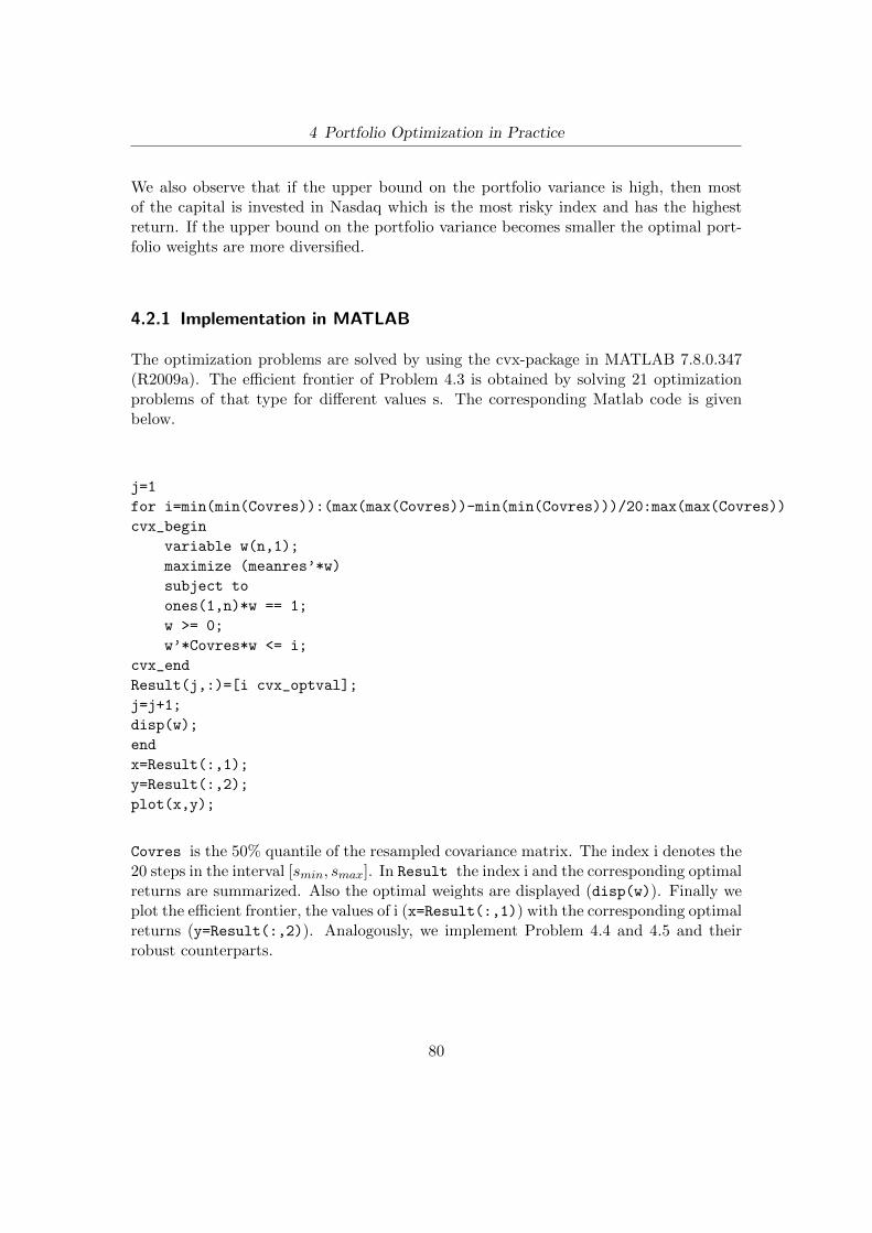
4 Portfolio Optimization in Practice
We also observe that if the upper bound on the portfolio variance is high, then mostof the capital is invested in Nasdaq which is the most risky index and has the highestreturn. If the upper bound on the portfolio variance becomes smaller the optimal port-folio weights are more diversified.
4.2.1 Implementation in MATLAB
The optimization problems are solved by using the cvx-package in MATLAB 7.8.0.347(R2009a). The efficient frontier of Problem 4.3 is obtained by solving 21 optimizationproblems of that type for different values s. The corresponding Matlab code is givenbelow.
j=1
for i=min(min(Covres)):(max(max(Covres))-min(min(Covres)))/20:max(max(Covres))
cvx_begin
variable w(n,1);
maximize (meanres’*w)
subject to
ones(1,n)*w == 1;
w >= 0;
w’*Covres*w <= i;
cvx_end
Result(j,:)=[i cvx_optval];
j=j+1;
disp(w);
end
x=Result(:,1);
y=Result(:,2);
plot(x,y);
Covres is the 50% quantile of the resampled covariance matrix. The index i denotes the20 steps in the interval [smin, smax]. In Result the index i and the corresponding optimalreturns are summarized. Also the optimal weights are displayed (disp(w)). Finally weplot the efficient frontier, the values of i (x=Result(:,1)) with the corresponding optimalreturns (y=Result(:,2)). Analogously, we implement Problem 4.4 and 4.5 and theirrobust counterparts.
80

4 Portfolio Optimization in Practice
4.3 Comparison: Classical optimization problems with therobust counterparts
In this section we compare the classical mean-variance optimization problems with theirrobust counterparts.
4.3.1 Uncertainty in the expected returns
First we consider Problem 4.3. For the robust counterpart, we assume that the expectedreturns are uncertain and lie in the following uncertainty set:
U(µr) ={µr = (µi) : µLi ≤ µi ≤ µUi , i = 1, . . . , n
}(4.6)
with the lower and upper bounds µLi and µUi , ∀i.
The formulation of the robust counterpart of Problem 4.3 is
maxw
minµr∈U(µr)
µ′rw (4.7)
s.t. e′w = 1
w′Σw ≤ swi ≥ 0, ∀i.
See also Problem 3.1, Section 3.2.1.
The worst case for the expected returns is µLr = (µL1 , . . . , µLn) and we get the following
robust optimization problem:
maxw
(µLr )′w (4.8)
s.t. e′w = 1
w′Σw ≤ swi ≥ 0, ∀i.
81

4 Portfolio Optimization in Practice
By bootstrapping from the historical data as described in the beginning of this chapterwe get the following lower bounds of the expected returns as 25% quantiles of the sampleddata
µLr =
0.0011314630.00077159190.00040588090.0007871138−0.0014519829
(4.9)
and the following upper bounds as 75% quantiles of the sampled data
µUr =
0.0025735380.00178142870.00141115490.0021264350−0.0001566744
. (4.10)
We have solved Problem 4.3 and its robust counterpart for 21 values of parameter s lyingin the interval [smin, smax], computed as described above.
The composition of the optimal portfolios for the robust optimization Problem 4.8 isillustrated in the following graphic. The composition of portfolios belonging to the effi-cient frontier of the corresponding Problem 4.3 is depicted in Figure 4.12.
Figure 4.15: Composition of efficient portfolios for Problem 4.8
82

4 Portfolio Optimization in Practice
With the highest level s = 0.0011 for the risk, everything is invested in Nasdaq, themost risky index. If the level for the risk is smaller then the optimal weights are morediversified, but the robust weights are a little bit more concentrated in Nasdaq than theclassical ones. The optimal value for the maximized reward is higher for the classicaloptimization problem than for the robust one, just as expected: in the robust optimiza-tion problem we use the worst case estimations for the asset returns, which clearly leadto a smaller portfolio return. We assume uncertainty in the expected returns only, sothe uncertainty does not affect the feasibility of the solution and there exists no solutionfor a level of risk lower than 0.00016516.
The following picture shows the efficient frontiers where the blue line corresponds tothe classical mean-variance optimization problem and the green one corresponds to therobust counterpart.
Figure 4.16: Classical and robust efficient frontiers for Problem 4.3 (blue) and Problem4.8 (green)
We can see that the robust efficient frontier lies below the classical one which means,that the robust optimal portfolio for a certain level of risk has a smaller reward than theportfolio on the classical efficient frontier. This fact is already commented above.
83

4 Portfolio Optimization in Practice
The following table shows the optimal solutions for the classical optimization Problem4.3 and its robust counterpart for some upper bounds values s on the risk.
classical robusts w optimal return w optimal return
0.00010967 No solution exists! -Inf No solution exists! -Inf
0.00016516
0.18000.30420.26770.17930.0688
0.00115956
0.17340.31080.27570.17430.0658
0.000589611
0.00033164
0.43520.29700.00000.26780.0000
0.00156249
0.44680.34690.00000.20630.0000
0.000935551
0.00083109
0.85470.00000.00000.14530.0000
0.00177877
0.86160.06230.00000.07610.0000
0.00108284
0.00094207
0.91860.00000.00000.08140.0000
0.00180333
0.92010.02280.00000.05710.0000
0.00110359
0.0011
1.00000.00000.00000.00000.0000
0.00183463
1.00000.00000.00000.00000.0000
0.00113146
Table 4.3: Solutions of Problem 4.3 and Problem 4.8
84

4 Portfolio Optimization in Practice
4.3.2 Uncertainty in the expected returns and the covariance matrix:Simple case
Next we compare Problem 4.4 with the robust counterpart:
minw
maxΣ∈U(Σ)
w′Σw (4.11)
s.t. e′w = 1
minµr∈U(µr)
µ′rw ≥ m
wi ≥ 0, ∀i
with the uncertainty set 4.6 for the expected returns and the uncertainty set for thecovariance matrix given as
U(Σ) ={
Σ = (Σij) : Σ ≤ Σ ≤ Σ, i, j = 1, . . . , n}
(4.12)
where the lower bound Σ = (Σij) and the upper bound Σ = (Σij) for the covariancematrix are obtained as 25% and 75% quantiles of the resampled data.
The lower and upper bounds Σ and Σ for the covariance matrix for all i, j = 1, . . . , 5.
Σ =
0.001035060 −0.000017004 −0.000017262 −0.000022645 −0.000021411−0.000017004 0.000524554 −0.000011390 −0.000015934 −0.000014725−0.000017262 −0.000011390 0.000523608 −0.000016311 −0.000015499−0.000022645 −0.000015934 −0.000016311 0.000949508 −0.000021178−0.000021411 −0.000014725 −0.000015499 −0.000021178 0.000892139
(4.13)
Σ =
0.0011901086 0.0000168514 0.0000164742 0.0000222886 0.00002239940.0000168514 0.0005993715 0.0000121208 0.0000152054 0.00001551350.0000164742 0.0000121208 0.0006138156 0.0000160002 0.00001621530.0000222886 0.0000152054 0.0000160002 0.0010674866 0.00001902760.0000223994 0.0000155135 0.0000162153 0.0000190276 0.0010142965
(4.14)
These matrices Σ and Σ are positive definite. So we do not need an approximation.
85

4 Portfolio Optimization in Practice
If we optimize with the worst case of the covariance matrix, which is Σ, we get thefollowing robust optimization problem:
minww′Σw (4.15)
s.t. e′w = 1
µ′rw ≥ mwi ≥ 0, ∀i
This problem is of the same type as a classical variance minimization problem, and canbe solved by standard methods, see also Problem 3.14, Section 3.2.2. We solve thisproblem for 20 different values of parameter m in the interval [−0.00078726, 0.0018] asdescribed in Section 4.2.
The composition of the efficient portfolios of Problem 4.4 is depicted in Figure 4.13.The allocation of the weights of its robust counterpart, Problem 4.11 is illustrated in thefollowing graphic.
Figure 4.17: Composition of efficient portfolios for Problem 4.11
If we compare Figure 4.13 and Figure 4.17 and consider for example the level of m =0.001, we can observe, that the efficient portfolio of the robust mean-variance optimiza-tion problem is less diversified, because we invest in Nasdaq, S&P 500 and Dax only,
86

4 Portfolio Optimization in Practice
whereas in the efficient portfolio of the classical mean-variance optimization problem weinvest in all indices.
The results of the classical and the robust optimization problems are listed in the fol-lowing table.
classical robustm w optimal risk w optimal risk
-0.00078726
0.13860.27420.27190.15330.1620
0.000153829
0.13560.27910.27210.15260.1606
0.000177634
0.00078587
0.13850.27420.27200.15330.1620
0.000153829
0.24230.35280.20770.19720.0000
0.00022433
0.00091697
0.13860.27420.27190.15330.1620
0.000153829
0.39450.38430.00000.22120.0000
0.00033752
0.0010
0.15920.28900.26980.16620.1158
0.00015662
0.76380.13290.00000.10330.0000
0.000723623
0.0012
0.18370.30680.26750.18150.0605
0.000167259 No solution exists! +Inf
Table 4.4: Solutions of Problem 4.4 and Problem 4.11
By comparing Table 4.4 and Table 4.3 we can see that the differences between the robustand the classical efficient portfolios are more pronounced in this case when we take into
87

4 Portfolio Optimization in Practice
account both the uncertainty in expected returns and also in the covariance matrix. Alsoin this case we observe that the optimal weights of the robust optimization problem aremore concentrated on certain indices while the weights of the classical portfolio opti-mization problem are more diversified. If the level of the prescribed reward is low, weinvest in all of the five indices with the most percentages in S&P 500 and FTSE becausethey have the smallest risk. From a level m = 0.0012 upwards there exists no feasiblesolution for the robust problem because we assume that the worst case for the expectedreturns occurs. If we compare the optimal values we can see that the minimized riskof the classical problem is lower than its robust counterpart. This is due to the worstcase assumption for the covariance matrix. We can see these the efficient frontiers of therobust and classical problem in the following picture.
Figure 4.18: Classical and robust efficient frontiers for Problem 4.4 (blue) and Problem4.11 (green)
The efficient frontier of the robust optimization problem is below and to the right of theclassical one.
88

4 Portfolio Optimization in Practice
4.3.3 Uncertainty in the expected returns and the covariance matrix:General case
In our previous chapter we explained that in general lower bounds Σij for the covariancesof asset i and j, 1 ≤ i, j ≤ 5, do not yield a positive definite matrix (Σ)1≤i,j≤5 and henceΣ cannot be used as a worst case approximation for the covariance matrix Σ. Thereforewe consider the robust risk-adjusted optimization problem with the general case for theuncertainty set of the covariance matrix, i.e., the robust counterpart of Problem 4.5.
maxw
{min
µr∈U(µr)µ′rw − c max
Σ∈U(Σ)w′Σw
}(4.16)
s.t. e′w = 1
wi ≥ 0, ∀i.
Consider the uncertainty set 4.6 for the expected returns, the uncertainty set 4.12 forthe covariance matrix and the dual variables Λ and Λ corresponding to the restrictionsΣ ≤ Σ and Σ ≤ Σ. As shown in Section 3.2.2. (Problem 3.22) the robust optimizationProblem 4.16 is equivalent to the following problem.
maxw,Λ,Λ
{(µLr )′w − c(
⟨Λ,Σ
⟩− 〈Λ,Σ〉)
}(4.17)
s.t. e′w = 1
wi ≥ 0, ∀iΛ ≥ 0, Λ ≥ 0(
Λ− Λ ww′ 1
)� 0.
We have solved this optimization problem by using the cvx-package of MATLAB 7.8.0.347(R2009).
For the optimal weights of Problem 4.5, see Figure 4.14, for the composition of efficientportfolios of Problem 4.17 see the following graphic.
89

4 Portfolio Optimization in Practice
Figure 4.19: Composition of efficient portfolios for Problem 4.17
We consider the efficient frontier of Problem 4.5 and 4.17.
Figure 4.20: Classical and robust efficient frontiers for Problem 4.5 (blue) and Problem4.17 (green)
90

4 Portfolio Optimization in Practice
The robust efficient frontier of the general case lies below the classical one, and this issimilar to pictures we have already seen when comparing the robust and classical coun-terpart for other models.
The following table shows the optimal weights of Problem 4.5 and 4.17 with the returnand risk of each efficient portfolio.
classical robustc w return risk w return risk
0.00
1.00000.00000.00000.00000.0000
0.001834631 0.001108555
1.00000.00000.00000.00000.0000
0.001131463 0.001201982
0.25
0.83970.00000.00000.16030.0000
0.001773003 0.00080745
0.70020.17610.00000.12370.0000
0.001025571 0.00062708
0.75
0.47350.25920.00000.26730.0000
0.001584611 0.00035819
0.39410.38460.00000.22130.0000
0.00091685 0.00033737
1.50
0.33450.32340.10050.24160.0000
0.001437368 0.00024715
0.28070.36310.15170.20450.0000
0.00082033 0.00024357
3.50
0.23790.32560.22860.20790.0000
0.001353618 0.00019522
0.21310.34520.25000.19170.0000
0.00075984 0.00021476
Table 4.5: Solutions of Problem 4.5 and Problem 4.17
We can see that the optimal robust portfolio is mainly invested in Nasdaq and a little bit
91

4 Portfolio Optimization in Practice
in S&P 500 while the optimal classical portfolio invests even more in Nasdaq. Nothingis invested in Nikkei 225 because of its negative expected return. If the risk-aversion pa-rameter c is small, the optimal robust and classical portfolios invest most of the capitalin Nasdaq. The weights get more diversified while c increases.
4.3.4 Stability of the optimization problems
The goal of the following numerical experiments is the investigation of the stability ofclassical and robust optimization problems.In practice, it can often happen that we have wrong estimates for the expected returnsand covariance matrices. Since small fluctuations in the input parameters influencethe solutions of the problem, wrong estimations would probably lead to bad solutions.In this context the robust portfolio optimization might be an alternative to classicalmean-variance optimization. To illustrate this alternative, we discuss the solution ofthree types of problems: the classical mean-variance optimization, the robust mean-variance optimization with uncertainty in the asset returns and the robust mean-varianceoptimization with uncertainty in the asset returns and in the covariance matrix (simplecase) as described in Section 4.3.2. The optimal portfolios are denoted by wc, wR1 andwR2, respectively. They are summarized in the following table.
wc wR1 wR2
0.7026 0.7148 0.67870.0776 0.2319 0.25430.0000 0.0000 0.00000.2198 0.0532 0.06710.0000 0.0000 0.0000
Table 4.6: Optimal weights of Problem 4.3 and its robust counterparts
Let us consider the performance of these three portfolios for real values µ0 and Σ0 ofexpected returns and covariance matrix. These values are in general not equal to theestimators. We compare the returns µ′0wc, µ
′0wR1 and µ′0wR2 of the classical and ro-
bust optimal portfolios, respectively. Analogously, we compare the variances w′cΣ0wc,w′R1ΣwR1 and w′R2Σ0wR2 of the classical and robust optimal portfolios. If the robustoptimization problem gets a higher reward and a lower risk, then the robust optimization
92

4 Portfolio Optimization in Practice
would be an alternative to the classical optimization model in this case.
Let us consider different return vectors and covariance matrices from the correspondinguncertainty sets as representatives of real values µ0 and Σ0. We pick up 20 vectorsµi, 1 ≤ i ≤ 20, randomly and uniformly distributed over the (µLr , µ
Ur ) given in 4.9,
4.10 where the selection is done independently for each index. Analogously, we selectσij ∈ (Σij ,Σij) randomly and uniformly distributed for i, j = 1, . . . , 5 and repeat thisprocess 20 times to generate the representatives of the real covariance matrix. The ma-trices (σij) are approximated by positive definite matrices as described in Section 4.1, ifnecessary. The results of this experiment are shown in Table 4.7.
reward risk
µ′iwc µ′iwR1 µ′iwR2 w′cΣiwc w′R1ΣiwR1 w′R2ΣiwR2
0.001061001 0.001073631 0.001058443 0.0005511491 0.0005521375 0.00050663740.001077957 0.001090796 0.001075445 0.0005555832 0.0005563026 0.00051057720.001094931 0.001105641 0.001090337 0.0005595174 0.0005602688 0.00051435300.001106748 0.001117025 0.001101646 0.0005629032 0.0005635259 0.00051746680.001121509 0.001129687 0.001114333 0.0005708408 0.0005711929 0.00052475430.001133438 0.001141012 0.001125579 0.0005792811 0.0005796031 0.00053267980.001149187 0.001155050 0.001139597 0.0005809381 0.0005812734 0.00053426480.001178473 0.001183283 0.001167751 0.0005852538 0.0005855010 0.00053823270.001216752 0.001219548 0.001203668 0.0006000069 0.0005999404 0.00055189120.001245978 0.001246654 0.001230833 0.0006034154 0.0006032613 0.00055506380.001275651 0.001277930 0.001261622 0.0006067427 0.0006065504 0.00055819280.001300774 0.001301317 0.001285071 0.0006162982 0.0006160385 0.0005671602
0.001403578 0.001400707 0.001383792 0.0006180100 0.0006176606 0.00056869960.001479743 0.001471578 0.001454361 0.0006216076 0.0006211292 0.00057200070.001733949 0.001716704 0.001697086 0.0006277695 0.0006271607 0.00057772330.002060558 0.002025411 0.002004609 0.0006342732 0.0006336522 0.00058387260.002160838 0.002123019 0.002102007 0.0006381557 0.0006374667 0.00058749210.002268360 0.002226652 0.002204519 0.0006399795 0.0006393226 0.00058924730.002301245 0.002259318 0.002236671 0.0006456496 0.0006449328 0.00059450410.002365520 0.002320049 0.002297019 0.0006517101 0.0006508782 0.0006000738
Table 4.7: Comparison of return and risk for classical and robust optimal portfolios
In 60% of the considered cases, the portfolio wR1 has the highest reward. When the”real” returns are high, then portfolio wc performs better in terms of total return. This
93

4 Portfolio Optimization in Practice
behavior is understandable and plausible because portfolio wc maximizes the total re-turn assuming that the expected assets returns are equal to the 50% quantiles of thebootstrapped values. By comparing the risk of portfolio wc and wR1, we can see thatin 12 of 20 cases portfolio wR1 has a lower risk. So we can conclude that in most ofthe cases the robust optimal portfolio wR1 outperforms the classical optimal portfoliowc. The reward of portfolio wR2 is the smallest one. In contrast, portfolio wR2 showsthe lowest risk in all cases. Summarizing we can conlude that the robust portfolio wR1
represent a good trade off between low risk and high return.
4.4 Conclusion
In this chapter we applied the models of classical and robust portfolio optimization pre-sented in the previous chapters to a portfolio of 5 assets: Nasdaq Composite, S&P 500,FTSE 100, Dax and Nikkei 225. The test bed and the analysis is similar to the computa-tional study of Tutuncu and Koenig [10]. They also compare the classical mean-varianceoptimization problems with their robust counterparts.
For the estimation of the expected returns and covariances, we apply a bootstrappingapproach similarly as Tutuncu and Koenig do. We use the historical data for bootstrap-ping and compute the sampled means and sampled covariances for the time series. Werepeat this procedure 3000 times, compute the 50%, 25% and 75% quantiles and getthe estimations of expected returns and covariance matrix as well as the correspondinglower and upper bounds for the uncertainty sets 4.6 and 4.12.
When comparing the efficient frontiers of the robust and classical optimization problems,we observe that the robust efficient frontier lies below the efficient frontier of the clas-sical Markowitz optimization. The reason is clear: the robust optimization model takesinto account the worst case realization of expected returns and covariance matrix. Theterms of the composition of optimal robust and classical portfolios we observe that inboth models most of the capital is investd in Nasdaq, if the upper bound on the varianceor the lower bound on the asset return is high. Especially in the optimization problemof minimizing the risk, the classical mean-variance optimal portfolio is more diversifiedthan the optimal robust portfolio.
Another result is that the robust optimal portfolio is more stable in the following sense.We compare the reward and the variance of two optimal robust portfolios and a classical
94

4 Portfolio Optimization in Practice
optimal portfolio for different realizations of return and covariance from the correspond-ing uncertainty sets. In 60% of the considered cases one of the robust portfolios performsbetter than the classical portfolio in terms of reward and/or variance.
Summarizing, our tests confirm that the robust portfolio optimization is a valuablealternative to the classical mean-variance optimization at least for risk-aware investors.
95

Bibliography
[1] Marc C. Steinbach:Markowitz Revisited: Single-Period and Multi-Period Mean-Variance Models,Society for Industrial and Applied Mathematics,Siam Review, 2001, vol. 43 (1), pp. 31-85
[2] Andreas Niedermayer, Daniel Niedermayer:Applying Markowitz’s Critical Line Algorithm,Discussion Paper, University of Bern, Department of Economics, 2006, dp0602
[3] Rainer E. Burkard:Einfuhrung in die mathematische OptimierungLecture notes, summer term 2007, TU Graz
[4] G. Cornuejols, R. Tutuncu:Optimization Methods in Finance.Cambridge University Press, 2007
[5] Frank J. Fabozzi, Petter N. Kolm, Dessislava Pachamanova:Robust Portfolio Optimization and ManagementJohn Wiley and Sons Inc, 2007
[6] Wei Jiao:Portfolio Resampling and Efficiency IssuesMaster thesis, Institute of Statistics and Economics, 2003
[7] Amit K. Sanyal, Teeyoung Lee, Melvin Leok, N. Harris McClamroch:Global optimum attitude estimation using uncertainty ellipsoids,Systems and Control Letters, 2008, vol. 57, pp. 236-245
96

Bibliography
[8] Lieven Vandenberghe, Stephen Boyd:Semidefinite Programming,Siam Rewiew, 1996, vol. 38, pp. 49-95
[9] Dimitris Bertsimas, Dessislava Pachamanova:Robust multiperiod portfolio management in the presence of transaction costs,Computers and Operations Research, 2008, vol. 35, pp. 3-17
[10] R.H.Tutuncu, M. Koenig:Robust Asset Allocation,Annals of Operations Research, Kluwer Academic Publisher, 2004,vol. 132, pp. 157-187
97


![An Exact Solution Approach for Portfolio Optimization ...1 Introduction Since Markowitz’ groundbreaking work in portfolio selection [22], portfolio optimization has been re-](https://img.dokumen.tips/doc/110x75/5f3092539655ea6a094da5aa/an-exact-solution-approach-for-portfolio-optimization-1-introduction-since-markowitza.jpg)