A Comparison of Solving the Poisson EquationUsing Several Numerical Methods

in Matlab and Octave on the Cluster mayaSarah Swatski, Samuel Khuvis, and Matthias K. Gobbert (gobbert@umbc.edu)

Department of Mathematics and Statistics, University of Maryland, Baltimore County

Technical Report HPCF–2014–10, www.umbc.edu/hpcf > Publications

Abstract

Systems of linear equations resulting from partial differential equations arise frequently in manyphenomena such as heat, sound, and fluid flow. We apply the finite difference method to the Poissonequation with homogeneous Dirichlet boundary conditions. This yields in a system of linear equationswith a large sparse system matrix that is a classical test problem for comparing direct and iterative linearsolvers. We compare the performance of Gaussian elimination, three classical iterative methods, and theconjugate gradient method in both Matlab and Octave. Although Gaussian elimination is fastest andcan solve large problems, it eventually runs out of memory. If very large problems need to be solved, theconjugate gradient method is available, but preconditioning is vital to keep run times reasonable. BothMatlab and Octave perform well with intermediate mesh resolutions; however, Matlab is eventually ableto solve larger problems than Octave and runs moderately faster.

Key words. Finite Difference Method, Iterative Methods, Matlab, Octave, Poisson Equation.

AMS subject classifications (2010). 65F05, 65F10, 65M06, 65Y04, 35J05.

1 Introduction

Partial differential equations (PDEs) are used in numerous disciplines to model phenomena such as heat,sound, and fluid flow. While many PDEs can be solved analytically, there are many that cannot be solvedanalytically or for which an analytic solution is far too costly or time-consuming. However, in many appli-cations, a numerical approximation to the solution is sufficient. Therefore, various numerical methods existto approximate the solutions to PDEs.

An ideal way to test a numerical method for PDEs is to use it on a PDE with a known analytical solution.That way, the true solution can be used to compute the error of the numerical method. By testing multiplenumerical methods on the same PDE and comparing their performance, we can determine which numericalmethods are most efficient.

The finite difference method uses finite differences to approximate the derivatives of a given function.After it is applied, we will have a system of linear equations for the unknowns. We will apply this method tothe Poisson equation, which is an elliptic PDE that is linear and has constant coefficients. It can be solvedanalytically using techniques such as separation of variables and Fourier expansions. We will use the systemof linear equations resulting from the finite difference method applied to the Poisson equation to comparethe linear solvers Gaussian elimination, classical iterative methods, and the conjugate gradient method. Thisproblem is a popular test problem and studied in [2, 3, 4, 7].

Matlab is the most commonly used commercial package for numerical computation in mathematics andrelated fields. However, Octave is a free software package that uses many of the same features and commandsas Matlab. Mathematics students typically take at least one course that utilizes a numerical computationsoftware, and Matlab is essentially the software of choice by professors and textbook authors alike. SinceOctave uses many of the same commands as Matlab and is free to the public, utilizing this software couldsave students and universities a significant amount of money paid in licenses to Matlab.

1

2 The Poisson Equation

We will test the methods on the Poisson equation with homogeneous Dirichlet boundary conditions given by

−4 u = f in Ω, (2.1)

u = 0 on ∂Ω, (2.2)

with right-hand side function

f(x, y) = −2π2 cos(2πx) sin2(πy)− 2π sin2(πx) cos(2πy),

on the two-dimensional unit square domain Ω = (0, 1)× (0, 1) ⊂ R2. In (2.1), the Laplace operator is definedby

4u =∂2u

∂x2+∂2u

∂y2

and ∂Ω in (2.2) represents the boundary of the domain Ω. This problem has a closed-form true solution of

u(x, y) = sin2(πx) sin2(πy). (2.3)

This problem is discussed in Section 3 of [1] and Section 8.1 of [7].

3 The Finite Difference Method

We first define a grid of mesh points with uniform mesh spacing h = 1N+1 . Thus, our grid can be represented

by Ωh = (xi, yi) = (ih, jh), i, j = 0, . . . , N + 1. We apply the second-order finite difference approximation(given as (8.1.3) on page 546 of [7]) to the x-derivative at all interior points of Ωh. This results in an equationthat approximates the x-derivative of u at a given (xi, yj) through evaluating u at (xi−1, yj), (xi, yj), and(xi+1, yj). A similar equation results by applying the second-order finite difference approximation to they-derivative at all interior points of Ωh. These equations are explicitly stated as (3) and (4) in Section 3 of [1].Substituting these results in (2.1) produces a system of equations for the approximation of the unknownsui,j ≈ u(xi, yj). Since the boundary conditions give u0,j = ui,0 = uN+1,j = ui,N+1 = 0, we see that

− ui−1,j − ui,j−1 + 4ui,j − ui+1,j − ui,j+1 = h2fi,j i, j = 1, . . . , N, (3.1)

where fi,j = f(xi, yj) for short.When N = 3, we obtain the nine equations

4u1,1 − u2,1 − u1,2 = h2f1,1, (3.2)−u1,1 + 4u2,1 − u3,1 − u2,2 = h2f2,1, (3.3)

− u2,1 + 4u3,1 − u3,2 = h2f3,1, (3.4)−u1,1 + 4u1,2 − u2,2 − u1,3 = h2f1,2, (3.5)

− u2,1 − u1,2 + 4u2,2 − u3,2 − u2,3 = h2f2,2, (3.6)− u3,1 − u2,2 + 4u3,2 − u3,3 = h2f3,2, (3.7)

− u1,2 + 4u1,3 − u2,3 = h2f1,3, (3.8)− u2,2 − u1,3 + 4u2,3 − u3,3 = h2f2,3, (3.9)

− u3,2 − u2,3 + 4u3,3 = h2f3,3. (3.10)

When N = 3, we see that (3.2) through (3.10) are linear in ui,j . Extending this for any N , we see that theN2 equations produced from (3.1) will also be linear in ui,j . Therefore this problem can be organized into

Au = b, with dimension N2 where A ∈ RN2×N2

and u,b ∈ RN2

. Since the boundary values are provided,

2

there will be exactly N2 unknowns. For this system, we see that

A =

S −I−I S −I

. . .. . .

. . .

−I S −I−I S

∈ RN2×N2

, where S =

4 −1−1 4 −1

. . .. . .

. . .

−1 4 −1−1 4

∈ RN×N ,

I is the N × N identity matrix, and bm = h2fi,j where m = i + (j − 1)N . To produce A in Matlab andOctave, we note representation of A as the sum of two Kronecker products. That is, A=I⊗T+T⊗ I whereI is the N ×N identity matrix and T ∈ RN×N is of the same form as S with 2’s on the diagonal instead of4’s.

Clearly, A is symmetric since A = AT . A is also positive definite because all eigenvalues are positive.This is a result of the Gershgorin disk theorem stated on pages 482-483 of [7]. The 1st and Nth Gershgorindisks, corresponding to the 1st and Nth rows of A, are centered at a11 = aNN = 4 on the complex planeand have radius r = 2. The kth Gershgorin disk, corresponding to the kth row of A where 2 ≤ k ≤ N − 1,is centered at akk = 4 on the complex plane with radius r ≤ 4. Since A is symmetric, all eigenvalues arereal, therefore we know that the eigenvalues, λ, satisfy 0 ≤ λ ≤ 8. However, A is non-singular, therefore weknow λ 6= 0 [7]. Therefore, all eigenvalues are positive, thus the matrix A is positive definite.

In order to discuss the convergence of the finite difference method, we must obtain the finite differenceerror. This error is given by the difference between the true solution u(x, y) defined in (2.3) and the numericalsolution uh defined on the mesh points where uh(xi, yj) = ui,j . We will use the L∞(Ω) norm defined by||u − uh||L∞(Ω) = sup(x,y)∈Ω |u(x, y) − uh(x, y)| discussed in [1] to compute this error. The finite difference

theory predicts that the quantity ||u − uh||L∞(Ω) ≤ Ch2 as h → 0, where C is a constant independent ofh [1]. As a result, for sufficiently small values of h, we suspect that the ratio of errors between consecutivemesh resolutions is

Ratio =||u− u2h||L∞(Ω)

||u− uh||L∞(Ω)≈ C(2h)2

Ch2= 4.

Thus, the finite difference method is second-order convergent if the ratio tends to 4 as N increases [1]. Wewill print this ratio in our tables so that we can discuss the convergence of the method.

4 The Computing Environment

The UMBC High Performance Computing Facility (HPCF) is the community-based, interdisciplinary corefacility for scientific computing and research on parallel algorithms at UMBC. The current machine in HPCFis the 240-node distributed-memory cluster maya. The newest part of the cluster are the 72 nodes with twoeight-core 2.6 GHz Intel E5-2650v2 Ivy Bridge CPUs and 64 GB memory that include 19 hybrid nodes withtwo state-of-the-art NVIDIA K20 GPUs (graphics processing units) designed for scientific computing and19 hybrid nodes with two cutting-edge 60-core Intel Phi 5110P accelerators. All nodes are connected viaInfiniBand to a central storage of more than 750 TB. The calculations in this report were performed onone node with two eight-core 2.6 GHz Intel E5-2650v2 Ivy Bridge CPUs and 64 GB memory using MatlabR2014a (8.3.0.532) and GNU Octave version 3.8.1.

4.1 Matlab

“Matlab is a high-level language and interactive environment for numerical computation, visualization, andprogramming,” as stated on its webpage www.mathworks.com. Matlab is available for purchase through itswebpage as a student version or for institutional licensing at considerable cost. The software was createdby Cleve Moler, a numerical analyst at the University of New Mexico’s Computer Science Department. Theinitial goal was to be able to make LINPACK and EISPACK more easily accessible by students, but it grewwhen its potential was recognized and Mathworks was established in 1983 [1]. The key features include itshigh-level language, interactive environment, mathematical functions, and built-in graphics.

3

4.2 Octave

“GNU Octave is a high-level interpreted language, primarily intended for numerical computations,” as statedon its webpage www.octave.org. It can be downloaded for free from http://sourceforge.net/projects/

octave. The software was developed by John W. Eaton, for use with an undergraduate textbook on chemicalreaction design. The capabilities of Octave grew when redevelopment was necessary, and its developmentbecame a full-time project in 1992. The main features of Octave are similar to Matlab, as it has an interactivecommand line interface and graphics capabilities.

5 Matlab Results

We will now solve the linear system produced from the Poisson Equation in Matlab R2014a using thevarious numerical methods. For Gaussian elimination with dense storage, we will use the code availablewith [1]. Since the code is written in sparse storage, for our calculations in dense storage we will simplyinsert A=full(A) after line 12 in the code. Sparse storage is here shorthand for using sparse storage modeof an array, in which only non-zero elements are stored. By contrast, in dense storage mode, all elements ofthe array are stored, whatever their value.

For the classical iterative methods, we will write a function classiter to solve the system using theJacobi method, the Gauss-Seidel method, and the successive overrelaxation (SOR(ω)) method. Each of themethods can be written in the form Mx(k+1) = Nx(k) + b where the splitting matrix M depends on themethod and N = M − A, and x(k) is the kth iterate [7]. As a result, we can set up the splitting matrixM depending on the method and use the same code to compute the iterations. The function classiter

takes the following input: the system matrix A, right-hand side vector b, tolerance tol, maximum number ofiterations maxit, a parameter imeth telling the function which method to use, the SOR relaxation parameterω, and an initial guess x(0). The splitting matrix M is then defined by the following: for the Jacobi method,M contains the diagonal elements of the system matrix A, M=spdiags(diag(A),[0],N,N); for the Gauss-Seidel method, M consists of the lower triangular and diagonal entries of A, M=tril(A); and for the SOR(ω)method, M is defined to be a matrix consisting of the inverse of ω multiplied by the diagonal elementsof A plus the lower triangular elements of A, M=(1/omega)*spdiags(diag(A),[0],N,N)+tril(A,-1) [7].The body of the function computes the iterates using the efficient update formula x=x+M\r, where r is theresidual value r = b −Ax. The function returns the final iterate x(k), a flag stating whether the methodsuccessfully converged to the desired tolerance before reaching the maximum number of iterations, the finalvalue of the relative residual ||r(k)||2/||b(k)||2, the number of iterations taken, and a vector of the residualsresvec where resvec(k)= ||r(k)||2. To run this function, we use the code for the conjugate gradient methodprovided with [1], replacing the call to pcg with a call to our function classiter. Therefore, line 16 of thecode becomes [u,flag,relres,iter,resvec] = classiter(A,b,tol,maxit,imeth,omega,x0).

For the final iterative method, the conjugate gradient method, we will use the code available with [1].For the conjugate gradient method with SSOR(ω) preconditioning, we must send pcg the SSOR splittingmatrix M. However, for an efficient implementation, we will send pcg the lower triangular factor M1 andupper triangular factor M2 such that M = M1M2 with

M1 =

√ω

2− ω

(1

ωD−E

)D−1/2, M2 =

√ω

2− ωD−1/2

(1

ωD− F

),

where D is a diagonal matrix, E is a strictly lower triangular matrix, and F is a strictly upper triangularmatrix such that A = D−E−F [7]. We note that M2 = MT

1 , and use this for more efficient code. Therefore,we obtain the code for the preconditioned conjugate gradient method in the following way. First, we computethe value of ω. Then, we compute the matrices D, D−1/2 and E. We do this by writing d = diag(A),D=spdiags(d,0,N^2,N^2), v = 1./sqrt(d), Ds = spdiags(v,0,N^2,N^2), and E=-tril(A,-1). Then wecompute M1 and M2 by M1 = sqrt(omega/(2-omega))*((1/omega)*D-E)*Ds and M2=M1’. Finally we callpcg with the code [u,flag,relres,iter,resvec] = pcg(A,b,tol,maxit,M1,M2,x0).

4

00.2

0.40.6

0.81

0

0.5

10

0.2

0.4

0.6

0.8

1

xy

u

00.2

0.40.6

0.81

0

0.5

10

1

2

3

4

x 10−3

xy

u−u h

(a) (b)

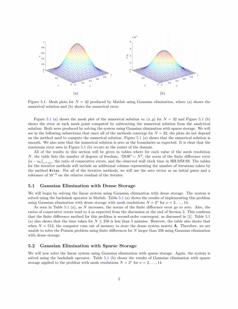
Figure 5.1: Mesh plots for N = 32 produced by Matlab using Gaussian elimination, where (a) shows thenumerical solution and (b) shows the numerical error.

Figure 5.1 (a) shows the mesh plot of the numerical solution vs. (x, y) for N = 32 and Figure 5.1 (b)shows the error at each mesh point computed by subtracting the numerical solution from the analyticalsolution. Both were produced by solving the system using Gaussian elimination with sparse storage. We willsee in the following subsections that since all of the methods converge for N = 32, the plots do not dependon the method used to compute the numerical solution. Figure 5.1 (a) shows that the numerical solution issmooth. We also note that the numerical solution is zero at the boundaries as expected. It is clear that themaximum error seen in Figure 5.1 (b) occurs at the center of the domain.

All of the results in this section will be given in tables where for each value of the mesh resolutionN , the table lists the number of degrees of freedom, “DOF”= N2, the norm of the finite difference error‖u− uh‖L∞(Ω)

, the ratio of consecutive errors, and the observed wall clock time in HH:MM:SS. The tablesfor the iterative methods will include an additional column representing the number of iterations taken bythe method #iter. For all of the iterative methods, we will use the zero vector as an initial guess and atolerance of 10−6 on the relative residual of the iterates.

5.1 Gaussian Elimination with Dense Storage

We will begin by solving the linear system using Gaussian elimination with dense storage. The system issolved using the backslash operator in Matlab. Table 5.1 (a) shows the results of implementing this problemusing Gaussian elimination with dense storage with mesh resolutions N = 2ν for ν = 2, . . . , 14.

As seen in Table 5.1 (a), as N increases, the norms of the finite difference error go to zero. Also, theratios of consecutive errors tend to 4 as expected from the discussion at the end of Section 3. This confirmsthat the finite difference method for this problem is second-order convergent, as discussed in [1]. Table 5.1(a) also shows that the time taken for N ≤ 256 is less than 5 minutes. However, the table also shows thatwhen N = 512, the computer runs out of memory to store the dense system matrix A. Therefore, we areunable to solve the Poisson problem using finite differences for N larger than 256 using Gaussian eliminationwith dense storage.

5.2 Gaussian Elimination with Sparse Storage

We will now solve the linear system using Gaussian elimination with sparse storage. Again, the system issolved using the backslash operator. Table 5.1 (b) shows the results of Gaussian elimination with sparsestorage applied to the problem with mesh resolutions N = 2ν for ν = 2, . . . , 14.

5

(a) Gaussian Elimination using Dense Storage in MatlabN DOF ‖u− uh‖ Ratio Time4 16 1.1673e-1 N/A <00:00:018 64 3.9152e-2 2.9813 <00:00:01

16 256 1.1267e-2 3.4748 <00:00:0132 1024 3.0128e-3 3.7399 <00:00:0164 4096 7.7812e-4 3.8719 <00:00:01

128 16384 1.9766e-4 3.9366 00:00:09256 65536 4.9807e-5 3.9685 00:04:41512 Out of Memory

1024 Out of Memory2048 Out of Memory4096 Out of Memory8192 Out of Memory

16384 Out of Memory

(b) Gaussian Elimination using Sparse Storage in MatlabN DOF ‖u− uh‖ Ratio Time4 16 1.1673e-1 N/A <00:00:018 64 3.9152e-2 2.9813 <00:00:01

16 256 1.1267e-2 3.4748 <00:00:0132 1024 3.0128e-3 3.7399 <00:00:0164 4096 7.7812e-4 3.8719 <00:00:01

128 16384 1.9766e-4 3.9366 <00:00:01256 65536 4.9807e-5 3.9685 <00:00:01512 262144 1.2501e-5 3.9843 <00:00:01

1024 1048576 3.1313e-6 3.9922 00:00:032048 4194304 7.8362e-7 3.9960 00:00:154096 16777216 1.9607e-7 3.9965 00:01:058192 67108864 4.9325e-8 3.9751 00:04:42

16384 Out of Memory

Table 5.1: Convergence results for the test problem in Matlab using Gaussian elimination with (a) densestorage and (b) sparse storage. For N = 8,192 using GE with sparse storage, the job was run on the usernode since it requires 74.6 GB of memory. Running this job on the compute node results in a runtime of6 minutes and 55 seconds.

As seen in Table 5.1 (b), as N increases, the norms of the finite difference error go to zero and theratios of consecutive errors tend to 4 implying convergence. Table 5.1 (b) also shows that the time taken forN ≤ 8,192 is less than 5 minutes. For N = 8,192, 74.6 GB of memory are required. A compute node onlyhas 64 GB of physical memory. If a job exceeds the 64 GB of physical memory then the the node will usethe swap space located on the hard drive. This results in a slower runtime of 6 minutes and 55 seconds. Byrunning on a user node with 128 GB of physical memory we can avoid the use of swap space to obtain aruntime of 4 minutes and 42 seconds. However, when N = 16,384, even the user node with 128 GB runs outof memory in the computation of the solution. Therefore, we are unable to solve the Poisson problem usingfinite differences for N larger than 8,192 using Gaussian elimination with sparse storage.

From the results in Tables 5.1 (a) and (b), we see that Gaussian elimination with sparse storage allows forthe linear system arising from the Poisson equation to be solved using larger mesh resolutions, N , withoutrunning out of memory. For those mesh resolutions for which both methods were able to solve the problem,N ≤ 256, we see that Gaussian elimination with sparse storage is faster than Gaussian elimination with densestorage. Therefore, we see the advantages of storing sparse matrices, namely matrix A from this problem,in sparse storage. Using sparse storage reduces the amount of memory required to store the matrix and

6

operations performed using matrices in sparse storage require less memory and are often faster. Therefore,we will utilize sparse storage for the remainder of the methods tested.

5.3 The Jacobi Method

We will begin by solving the linear system using the first of the three classical iterative methods tested, theJacobi method. Table 5.2 (a) shows the results of implementing this problem using the Jacobi method withmesh resolutions N = 2ν , for ν = 2, . . . , 14.

As seen in Table 5.2 (a), as N increases, the norms of the finite difference error appear to be going tozero and the ratios of consecutive errors appear to tend to 4 implying convergence second order convergence.Table 5.2 (a) also shows that the time taken for N ≤ 512 is less than 1 hour 18 minutes. However, whenN = 1,024, the Jacobi method begins to take an excessive amount of time to solve the problem. Therefore,we are unable to solve the Poisson problem using finite differences for N larger than 512 using the Jacobimethod.

5.4 The Gauss-Seidel Method

We will now solve the linear system using the second of the three classical iterative methods tested, theGauss-Seidel method. Table 5.2 (b) shows the results of implementing this problem using the Gauss-Seidelmethod with mesh resolutions N = 2ν , for ν = 2, . . . , 14.

As seen in Table 5.2 (b), as N increases, the norms of the finite difference error appear to be going tozero and the ratios of consecutive errors appear to tend to 4 implying second order convergence. Table 5.2(b) also shows that the time taken for N ≤ 1,024 is less than 12 hours. However, when N = 2,048, theGauss-Seidel method begins to take an excessive amount of time to solve the problem. Therefore, we areunable to solve the Poisson problem using finite differences for N larger than 2,048 using the Gauss-Seidelmethod.

5.5 The Successive Overrelaxation Method

We will now solve the linear system using the third of the three classical iterative methods tested, thesuccessive overrelaxation method (SOR(ω)). The optimal ω, ωopt = 2/(1 + sin(πh)), defined in [7] and [8]was used. Table 5.2 (c) shows the results of implementing this problem using the SOR(ωopt) method withmesh resolutions N = 2ν , for ν = 2, . . . , 14.

As seen in Table 5.2 (c), as N increases, ωopt tends to 2. We also note that the norms of the finite differenceerror appear to be going to zero while the ratios of consecutive errors appear to tend to 4 implying secondorder convergence. For the two finest mesh resolutions, the reduction in error appears slightly more erratic,which points to the tolerance of the iterative linear solver not being tight enough to ensure a sufficientlyaccurate solution of the linear system. Table 5.2 (c) also shows that the time taken for N ≤ 4,096 is lessthan 2 hours. However, when N = 8,192, the method begins to take an excessive amount of time to solvethe problem. Therefore, we are unable to solve the Poisson problem using finite differences for N larger than4,096 using the SOR(ωopt) method.

From the results in Tables 5.2 (a), (b) and (c), we see that the SOR(ωopt) method allows for the systemto be solved with larger mesh resolutions N than both the Jacobi and Gauss-Seidel methods. This is a resultof the fact that the number of iterations required to solve the linear system for a given mesh resolution Ndecreases when the method is changed from Jacobi to Gauss-Seidel to SOR(ωopt). Therefore, the SOR(ωopt)method is the best method among the three classical iterative methods tested. However, we see that none ofthe classical iterative methods has any advantage over Gaussian elimination, which as able to solve a largerproblem faster, provided sparse storage is used.

5.6 The Conjugate Gradient Method

We will now solve the linear system using the conjugate gradient method. Table 5.3 (a) shows the results ofthe conjugate gradient method applied to the problem with mesh resolutions N = 2ν for ν = 2, . . . , 14.

7

(a) Jacobi Method in MatlabN DOF ‖u− uh‖ Ratio #iter Time4 16 1.1673e-1 N/A 64 00:00:028 64 3.9151e-2 2.9814 214 <00:00:01

16 256 1.1266e-2 3.4751 769 <00:00:0132 1024 3.0114e-3 3.7411 2902 <00:00:0164 4096 7.7673e-4 3.8771 11258 00:00:01

128 16384 1.9626e-4 3.9577 44331 00:00:17256 65536 4.8397e-5 4.0551 175921 00:03:57512 262144 1.1089e-5 4.3646 700881 01:06:10

1024 Excessive Time required2048 Excessive Time required4096 Excessive Time required8192 Excessive Time required

16384 Excessive Time required

(b) Gauss-Seidel Method in MatlabN DOF ‖u− uh‖ Ratio #iter Time4 16 1.1673e-1 N/A 33 <00:00:018 64 3.9151e-2 2.9814 108 <00:00:01

16 256 1.1266e-2 3.4751 386 <00:00:0132 1024 3.0114e-3 3.7411 1452 <00:00:0164 4096 7.7673e-4 3.8771 5630 <00:00:01

128 16384 1.9626e-4 3.9577 22166 00:00:11256 65536 4.8398e-5 4.0551 87962 00:02:44512 262144 1.1089e-5 4.3645 350442 00:46:42

1024 1048576 1.7182e-6 6.4538 1398959 11:23:422048 Excessive Time required4096 Excessive Time required8192 Excessive Time required

16384 Excessive Time required

(c) Successive Overrelaxation Method (SOR(ωopt)) in MatlabN DOF ωopt ‖u− uh‖ Ratio #iter Time4 16 1.2596 1.1673e-1 N/A 14 <00:00:018 64 1.4903 3.9152e-2 2.9813 25 <00:00:01

16 256 1.6895 1.1267e-2 3.4749 47 <00:00:0132 1024 1.8264 3.0125e-3 3.7401 92 <00:00:0164 4096 1.9078 7.7785e-4 3.8729 181 <00:00:01

128 16384 1.9525 1.9737e-4 3.9410 359 <00:00:01256 65536 1.9758 4.9522e-5 3.9856 716 00:00:01512 262144 1.9878 1.2214e-5 4.0544 1429 00:00:12

1024 1048576 1.9939 2.8630e-6 4.2662 2861 00:01:332048 4194304 1.9969 5.5702e-7 5.1399 5740 00:13:224096 16777216 1.9985 4.6471e-7 1.1986 11559 01:48:068192 Excessive Time required

16384 Excessive Time required

Table 5.2: Convergence results for the test problem in Matlab using (a) the Jacobi method, (b) the Gauss-Seidel method, and (c) the SOR(ωopt) method. Excessive time corresponds to more than 12 hours wall clocktime.

8

(a) The Conjugate Gradient Method in MatlabN DOF ‖u− uh‖ Ratio #iter Time4 16 1.1673e-1 N/A 3 00:00:018 64 3.9152e-2 2.9813 10 <00:00:01

16 256 1.1267e-2 3.4748 24 <00:00:0132 1024 3.0128e-3 3.7399 48 <00:00:0164 4096 7.7811e-4 3.8719 96 <00:00:01

128 16384 1.9765e-4 3.9368 192 <00:00:01256 65536 4.9797e-5 3.9690 387 <00:00:01512 262144 1.2494e-5 3.9856 783 00:00:06

1024 1048576 3.1266e-6 3.9961 1581 00:00:462048 4194304 7.8019e-7 4.0075 3192 00:06:444096 16777216 1.9366e-7 4.0287 6452 00:53:308192 67108864 4.7375e-8 4.0878 13033 07:12:30

16384 Excessive Time required

(b) The Conjugate Gradient Method with SSOR(ωopt) Preconditioning in MatlabN DOF ωopt ‖u− uh‖ Ratio #iter Time4 16 1.2596 1.1673e-1 N/A 7 <00:00:018 64 1.4903 3.9153e-2 2.9813 9 <00:00:01

16 256 1.6895 1.1267e-2 3.4748 14 <00:00:0132 1024 1.8264 3.0128e-3 3.7399 19 <00:00:0164 4096 1.9078 7.7812e-4 3.8719 28 <00:00:01

128 16384 1.9525 1.9766e-4 3.9366 40 <00:00:01256 65536 1.9758 4.9811e-5 3.9683 57 <00:00:01512 262144 1.9878 1.2502e-5 3.9842 83 00:00:02

1024 1048576 1.9939 3.1321e-6 3.9917 121 00:00:102048 4194304 1.9969 7.8394e-7 3.9953 176 00:00:554096 16777216 1.9985 1.9620e-7 3.9957 256 00:05:218192 67108864 1.9992 4.9109e-8 3.9952 375 00:30:51

16384 268435456 1.9996 1.2301e-8 3.9923 548 03:07:29

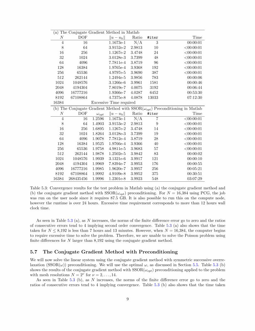
Table 5.3: Convergence results for the test problem in Matlab using (a) the conjugate gradient method and(b) the conjugate gradient method with SSOR(ωopt) preconditioning. For N = 16,384 using PCG, the jobwas run on the user node since it requires 87.5 GB. It is also possible to run this on the compute node,however the runtime is over 24 hours. Excessive time requirement corresponds to more than 12 hours wallclock time.

As seen in Table 5.3 (a), as N increases, the norms of the finite difference error go to zero and the ratiosof consecutive errors tend to 4 implying second order convergence. Table 5.3 (a) also shows that the timetaken for N ≤ 8,192 is less than 7 hours and 13 minutes. However, when N = 16,384, the computer beginsto require excessive time to solve the problem. Therefore, we are unable to solve the Poisson problem usingfinite differences for N larger than 8,192 using the conjugate gradient method.

5.7 The Conjugate Gradient Method with Preconditioning

We will now solve the linear system using the conjugate gradient method with symmetric successive overre-laxation (SSOR(ω)) preconditioning. We will use the optimal ω, as discussed in Section 5.5. Table 5.3 (b)shows the results of the conjugate gradient method with SSOR(ωopt) preconditioning applied to the problemwith mesh resolutions N = 2ν for ν = 2, . . . , 14.

As seen in Table 5.3 (b), as N increases, the norms of the finite difference error go to zero and theratios of consecutive errors tend to 4 implying convergence. Table 5.3 (b) also shows that the time taken

9

0 500 1000 1500 2000 2500 300010

−8

10−6

10−4

10−2

100

102

k−−

||r(k

) || 2/||b|

| 2

Relative Residual versus Iteration Number

Jacobi GS SOR CG PCG−SSOR

0 20 40 60 80 100

10−6

10−4

10−2

100

k−−

||r(k

) || 2/||b|

| 2

Relative Residual versus Iteration Number

Jacobi GS SOR CG PCG−SSOR

(a) (b)

Figure 5.2: The relative residual versus iteration number k for N = 32 for all iterative methods where “GS”represents Gauss-Seidel, “SOR” represents successive overrelaxation, “CG” represents conjugate gradient,and “PCG-SSOR” represents conjugate gradient with symmetric successive overrelaxation preconditioning.Figure (a) shows the graph to the maximum number of iterations required for all methods and (b) shows theplot to k = 100. The dashed black line represents the desired tolerance, 10−6. These figures were producedin Matlab.

for N ≤ 16,384 is less than 3 hours and 8 minutes. For N = 16,384 using PCG, the job required 87.5 GBof memory to run. This was completed in over 24 hours by using the swap space on a compute node. Byusing a user node with 128 GB of memory and thus not requiring the use of swap space, the runtime issignificantly reduced. However, when N = 32,768, the computer runs out of memory to store the systemmatrix A. Therefore, we are unable to solve the Poisson problem using finite differences for N larger than16,384 using the conjugate gradient method with SSOR(ωopt) preconditioning.

From the results in Tables 5.3 (a) and (b), we see that the conjugate gradient method with SSOR(ωopt)preconditioning converges with an order of magnitude reduction in iterations as well as run time. Thisdemonstrates that the added cost of preconditioning in each iteration is worth the cost. The results for con-jugate gradients both without and with preconditioning show that that their decreased memory requirementsallow to solve larger problems than Gaussian elimination. But only the preconditioned conjugate gradientmethod is efficient enough to solve the larger problems in reasonable amount of time.

5.8 A Comparison of the Iterative Methods

To compare all iterative methods graphically, we will plot the relative residuals ||r(k)||2/||b||2 versus theiteration number k for N = 32 in a semi-log plot shown in Figure 5.2 (a) and (b). This plot is produced usingthe semilogy command in Matlab. It is clear from Figure 5.2 (a) that the Jacobi and Gauss-Seidel methodstake far more iterations to converge than the remaining three iterative methods. Figure 5.2 (b) zooms inon the plot so that the behavior between SOR(ωopt), the conjugate gradient method, and the conjugategradient method with SSOR(ωopt) preconditioning can be compared. It is clear from Figure 5.2 (b) that theconjugate gradient method with SSOR(ωopt) preconditioning is superior to the conjugate gradient methodwithout preconditioning, which in turn is superior to SOR(ωopt). Figure 5.2 (b) also shows that the conjugategradient methods experience a slight increase in the relative residual within the first 10 iterations. However,once these iterations are complete, the superiority of the methods shine through in the quick convergencerate.

10

0

0.2

0.4

0.6

0.8

1

x

0

0.2

0.4

0.6

0.8

1

y

0

0.2

0.4

0.6

0.8

1

u

0

0.2

0.4

0.6

0.8

1

x

0

0.2

0.4

0.6

0.8

1

y

-0.001

0

0.001

0.002

0.003

0.004

u-uh

(a) (b)

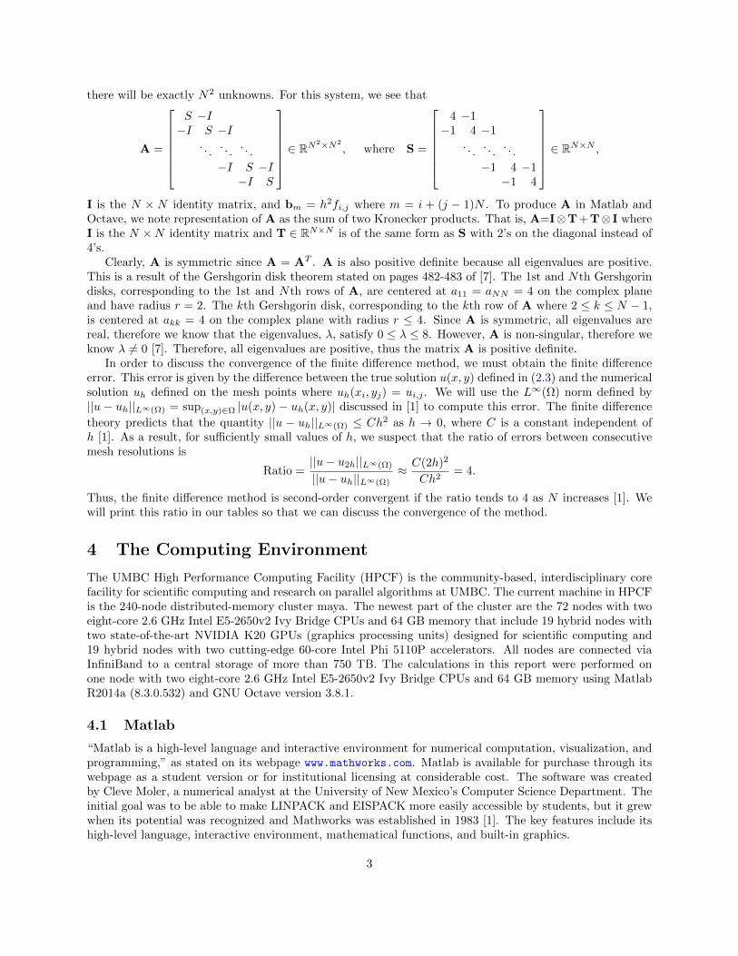
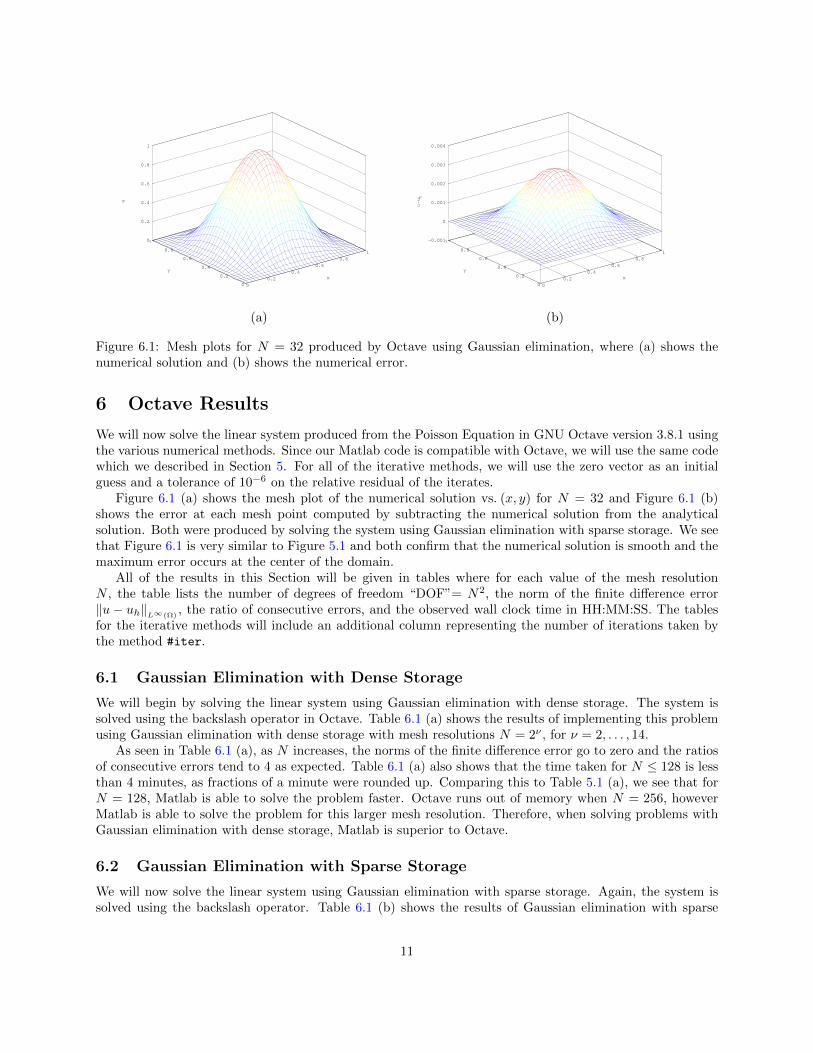
Figure 6.1: Mesh plots for N = 32 produced by Octave using Gaussian elimination, where (a) shows thenumerical solution and (b) shows the numerical error.

6 Octave Results

We will now solve the linear system produced from the Poisson Equation in GNU Octave version 3.8.1 usingthe various numerical methods. Since our Matlab code is compatible with Octave, we will use the same codewhich we described in Section 5. For all of the iterative methods, we will use the zero vector as an initialguess and a tolerance of 10−6 on the relative residual of the iterates.

Figure 6.1 (a) shows the mesh plot of the numerical solution vs. (x, y) for N = 32 and Figure 6.1 (b)shows the error at each mesh point computed by subtracting the numerical solution from the analyticalsolution. Both were produced by solving the system using Gaussian elimination with sparse storage. We seethat Figure 6.1 is very similar to Figure 5.1 and both confirm that the numerical solution is smooth and themaximum error occurs at the center of the domain.

All of the results in this Section will be given in tables where for each value of the mesh resolutionN , the table lists the number of degrees of freedom “DOF”= N2, the norm of the finite difference error‖u− uh‖L∞(Ω)

, the ratio of consecutive errors, and the observed wall clock time in HH:MM:SS. The tablesfor the iterative methods will include an additional column representing the number of iterations taken bythe method #iter.

6.1 Gaussian Elimination with Dense Storage

We will begin by solving the linear system using Gaussian elimination with dense storage. The system issolved using the backslash operator in Octave. Table 6.1 (a) shows the results of implementing this problemusing Gaussian elimination with dense storage with mesh resolutions N = 2ν , for ν = 2, . . . , 14.

As seen in Table 6.1 (a), as N increases, the norms of the finite difference error go to zero and the ratiosof consecutive errors tend to 4 as expected. Table 6.1 (a) also shows that the time taken for N ≤ 128 is lessthan 4 minutes, as fractions of a minute were rounded up. Comparing this to Table 5.1 (a), we see that forN = 128, Matlab is able to solve the problem faster. Octave runs out of memory when N = 256, howeverMatlab is able to solve the problem for this larger mesh resolution. Therefore, when solving problems withGaussian elimination with dense storage, Matlab is superior to Octave.

6.2 Gaussian Elimination with Sparse Storage

We will now solve the linear system using Gaussian elimination with sparse storage. Again, the system issolved using the backslash operator. Table 6.1 (b) shows the results of Gaussian elimination with sparse

11

(a) Gaussian Elimination using Dense Storage in OctaveN DOF ‖u− uh‖ Ratio Time4 16 1.1673e-1 N/A <00:00:018 64 3.9152e-2 2.9813 <00:00:01

16 256 1.1267e-2 3.4748 <00:00:0132 1024 3.0128e-3 3.7399 <00:00:0164 4096 7.7812e-4 3.8719 00:00:05

128 16384 1.9766e-4 3.9366 00:04:00256 out of memory512 out of memory

1024 out of memory2048 out of memory4096 out of memory8192 out of memory

16384 out of memory

(b) Gaussian Elimination using Sparse Storage in OctaveN DOF ‖u− uh‖ Ratio Time4 16 1.1673e-1 N/A <00:00:018 64 3.9152e-2 2.9813 <00:00:01

16 256 1.1267e-2 3.4748 <00:00:0132 1024 3.0128e-3 3.7399 <00:00:0164 4096 7.7812e-4 3.8719 <00:00:01

128 16384 1.9766e-4 3.9366 <00:00:01256 65536 4.9807e-5 3.9685 <00:00:01512 262144 1.2501e-5 3.9843 <00:00:01

1024 1048576 3.1313e-6 3.9922 00:00:062048 4194304 7.8362e-7 3.9960 00:00:374096 16777216 1.9607e-7 3.9966 00:04:218192 out of memory

16384 out of memory

Table 6.1: Convergence results for the test problem in Octave using Gaussian elimination with (a) densestorage and (b) sparse storage.

storage applied to the problem with mesh resolutions N = 2ν for ν = 2, . . . , 14.As seen in Table 6.1 (b), as N increases, the norms of the finite difference error go to zero and the ratios

of consecutive errors tend to 4 as expected. Table 6.1 (b) also shows that the time taken for N ≤ 4,096is less than 5 minutes. Comparing this to Table 5.1 (b), we see that for N ≤ 512, Octave was able tosolve the problem in almost the same amount of time as Matlab. However, for 1,024 ≤ N ≤ 4,096, Octaverequires almost twice the amount of time required by Matlab. Additionally, Octave runs out of memorywhen N = 8,192, but Matlab is able to solve the problem for this larger mesh resolution. Therefore, whensolving problems with Gaussian elimination with sparse storage with large mesh resolutions, Matlab shouldbe used.

From the results in Tables 6.1 (a) and (b), we see that Gaussian elimination with sparse storage allows forthe linear system arising from the Poisson equation to be solved using larger mesh resolutions, N , withoutrunning out of memory and is faster. Therefore, we will utilize sparse storage for the remainder of themethods tested.

12

6.3 The Jacobi Method

We will begin by solving the linear system using the first of the three classical iterative methods tested, theJacobi method. Table 6.2 (a) shows the results of implementing this problem using the Jacobi method withmesh resolutions N = 2ν , for ν = 2, . . . , 14.

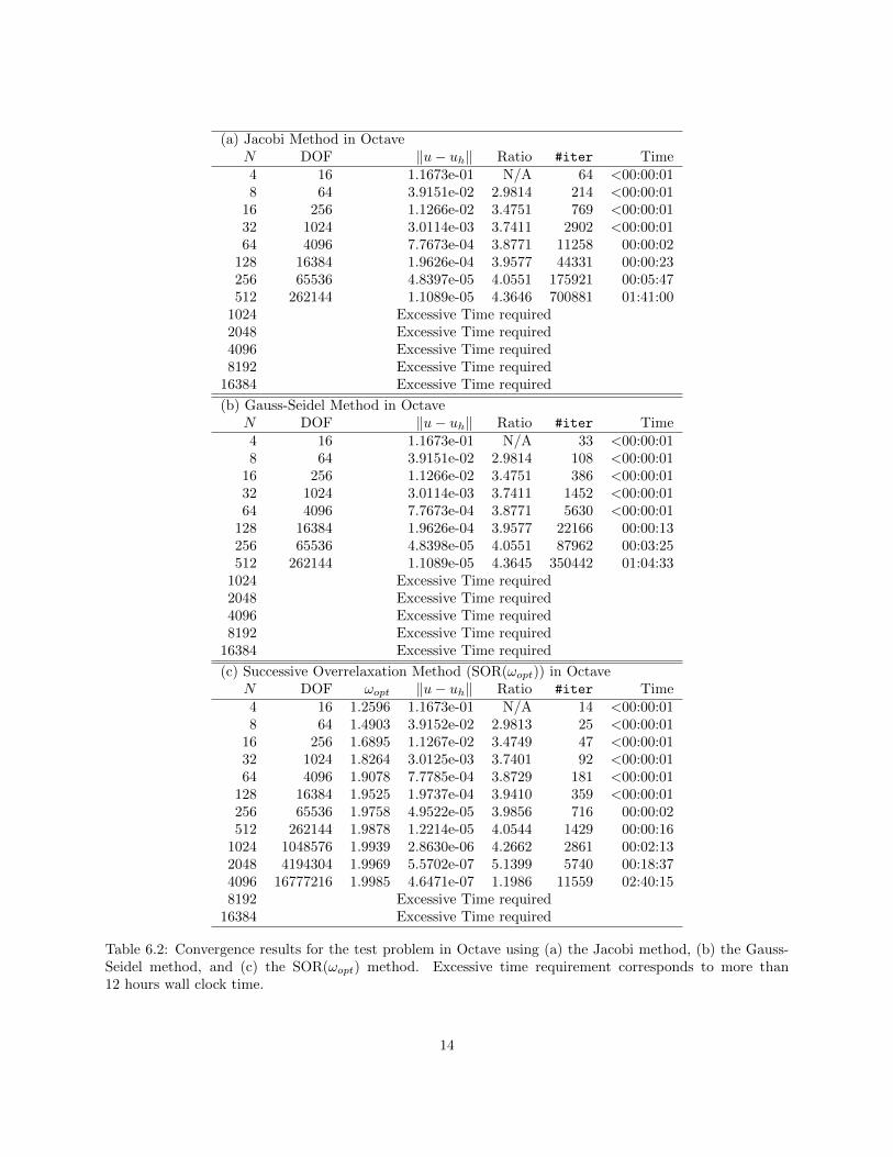
As seen in Table 6.2 (a), as N increases, the norms of the finite difference error appear to be going to zeroand the ratios of consecutive errors appear to tend to 4 implying second order convergence. Table 6.2 (a)also shows that the time taken for N ≤ 512 is less than 1 hour 42 minutes. Comparing this to Table 5.2 (a),we see that for N ≤ 32, Octave was able to solve the problem in almost the same amount of time as Matlab.However, when N ≥ 32, Octave takes almost two times the amount of time taken by Matlab to solve theproblem. Therefore, when solving problems with the Jacobi method using a large mesh resolution, Matlab issuperior to Octave. Also, as with Matlab, the table shows that when N = 1,024, the Jacobi method beginsto take an excessive amount of time to solve the problem.

6.4 The Gauss-Seidel Method

We will now solve the linear system using the second of the three classical iterative methods tested, theGauss-Seidel method. Table 6.2 (b) shows the results of implementing this problem using the Gauss-Seidelmethod with mesh resolutions N = 2ν , for ν = 2, . . . , 14.

As seen in Table 6.2 (b), as N increases, the norms of the finite difference error appear to be going to zeroand the ratios of consecutive errors appear to tend to 4 implying second order convergence. Table 6.2 (b)also shows that the time taken for N ≤ 512 is less than 1 hour and 5 minutes. Comparing this to Table 5.2(b), we see that for N ≤ 128, Octave was able to solve the problem in almost the same amount of time asMatlab. However, when N ≥ 256, Octave takes about one and a half times the amount of time taken byMatlab to solve the problem. Therefore, when solving problems with the Gauss-Seidel method using a largemesh resolution, Matlab is superior to Octave. Also, the table shows that when N = 1,024, the Gauss-Seidelmethod takes more time than we consider reasonable, while Matlab is able to return a result in a reasonableamount of time.

6.5 The Successive Overrelaxation Method

We will now solve the linear system using the third of the three classical iterative methods tested, thesuccessive overrelaxation method (SOR(ω)). The optimal ω, as discussed in Section 5.5ωopt = 2/(1+sin(πh))will be used. Table 6.2 (c) shows the results of implementing this problem using the SOR(ωopt) method withmesh resolutions N = 2ν , for ν = 2, . . . , 14.

As seen in Table 6.2 (c), as N increases, ωopt tends to 2. We also note that the norms of the finite differenceerror appear to be going to zero while the ratios of consecutive errors appear to tend to 4, implying secondorder convergence. For the two finest mesh resolutions, the reduction in error appears slightly more erratic,which points to the tolerance of the iterative linear solver not being tight enough to ensure a sufficientlyaccurate solution of the linear system. Table 6.2 (c) also shows that the time taken for N ≤ 4,096 is lessthan 2 hours 41 minutes. Comparing this to Table 5.2 (c), we see that for N ≤ 512, Octave was able tosolve the problem in almost the same amount of time as Matlab. However, when N ≥ 1,024, Octave takesbetween almost one and a half times the amount of time taken by Matlab to solve the problem. Also, similarto the Matlab results, the table shows that when N = 8,192, the SOR method begins to take an excessiveamount of time to solve the problem.

From the results in Tables 6.2 (a), (b) and (c), we see that the SOR(ωopt) method allows for the system tobe solved for larger mesh resolutions N than the Gauss-Seidel and Jacobi methods. Therefore, the SOR(ωopt)method is the best method among the three classical iterative methods tested.

6.6 The Conjugate Gradient Method

We will now solve the linear system using the conjugate gradient method. Table 6.3 (a) shows the results ofthe conjugate gradient method applied to the problem with mesh resolutions N = 2ν for ν = 2, . . . , 14.

13

(a) Jacobi Method in OctaveN DOF ‖u− uh‖ Ratio #iter Time4 16 1.1673e-01 N/A 64 <00:00:018 64 3.9151e-02 2.9814 214 <00:00:01

16 256 1.1266e-02 3.4751 769 <00:00:0132 1024 3.0114e-03 3.7411 2902 <00:00:0164 4096 7.7673e-04 3.8771 11258 00:00:02

128 16384 1.9626e-04 3.9577 44331 00:00:23256 65536 4.8397e-05 4.0551 175921 00:05:47512 262144 1.1089e-05 4.3646 700881 01:41:00

1024 Excessive Time required2048 Excessive Time required4096 Excessive Time required8192 Excessive Time required

16384 Excessive Time required

(b) Gauss-Seidel Method in OctaveN DOF ‖u− uh‖ Ratio #iter Time4 16 1.1673e-01 N/A 33 <00:00:018 64 3.9151e-02 2.9814 108 <00:00:01

16 256 1.1266e-02 3.4751 386 <00:00:0132 1024 3.0114e-03 3.7411 1452 <00:00:0164 4096 7.7673e-04 3.8771 5630 <00:00:01

128 16384 1.9626e-04 3.9577 22166 00:00:13256 65536 4.8398e-05 4.0551 87962 00:03:25512 262144 1.1089e-05 4.3645 350442 01:04:33

1024 Excessive Time required2048 Excessive Time required4096 Excessive Time required8192 Excessive Time required

16384 Excessive Time required

(c) Successive Overrelaxation Method (SOR(ωopt)) in OctaveN DOF ωopt ‖u− uh‖ Ratio #iter Time4 16 1.2596 1.1673e-01 N/A 14 <00:00:018 64 1.4903 3.9152e-02 2.9813 25 <00:00:01

16 256 1.6895 1.1267e-02 3.4749 47 <00:00:0132 1024 1.8264 3.0125e-03 3.7401 92 <00:00:0164 4096 1.9078 7.7785e-04 3.8729 181 <00:00:01

128 16384 1.9525 1.9737e-04 3.9410 359 <00:00:01256 65536 1.9758 4.9522e-05 3.9856 716 00:00:02512 262144 1.9878 1.2214e-05 4.0544 1429 00:00:16

1024 1048576 1.9939 2.8630e-06 4.2662 2861 00:02:132048 4194304 1.9969 5.5702e-07 5.1399 5740 00:18:374096 16777216 1.9985 4.6471e-07 1.1986 11559 02:40:158192 Excessive Time required

16384 Excessive Time required

Table 6.2: Convergence results for the test problem in Octave using (a) the Jacobi method, (b) the Gauss-Seidel method, and (c) the SOR(ωopt) method. Excessive time requirement corresponds to more than12 hours wall clock time.

14

(a) The Conjugate Gradient Method in OctaveN DOF ‖u− uh‖ Ratio #iter Time4 16 1.1673e-01 N/A 3 <00:00:018 64 3.9152e-02 2.9813 10 <00:00:01

16 256 1.1267e-02 3.4748 24 <00:00:0132 1024 3.0128e-03 3.7399 48 <00:00:0164 4096 7.7811e-04 3.8719 96 <00:00:01

128 16384 1.9765e-04 3.9368 192 <00:00:01256 65536 4.9797e-05 3.9690 387 <00:00:01512 262144 1.2494e-05 3.9856 783 00:00:07

1024 1048576 3.1266e-06 3.9961 1581 00:01:062048 4194304 7.8019e-07 4.0075 3192 00:10:084096 16777216 1.9354e-07 4.0311 6452 01:21:498192 67108864 4.6775e-08 4.1377 13033 11:06:22

16384 Excessive Time required

(b) The Conjugate Gradient Method with SSOR(ωopt) Preconditioning in OctaveN DOF ωopt ‖u− uh‖ Ratio #iter Time4 16 1.2596 1.1673e-01 N/A 7 <00:00:018 64 1.4903 3.9153e-02 2.9813 9 <00:00:01

16 256 1.6895 1.1267e-02 3.4748 14 <00:00:0132 1024 1.8264 3.0128e-03 3.7399 19 <00:00:0164 4096 1.9078 7.7812e-04 3.8719 28 <00:00:01

128 16384 1.9525 1.9766e-04 3.9366 40 <00:00:01256 65536 1.9758 4.9811e-05 3.9683 57 <00:00:01512 262144 1.9878 1.2502e-05 3.9842 83 00:00:02

1024 1048576 1.9939 3.1321e-06 3.9917 121 00:00:092048 4194304 1.9969 7.8394e-07 3.9953 176 00:00:574096 16777216 1.9985 1.9618e-07 3.9961 257 00:05:418192 67108864 1.9992 4.9102e-08 3.9953 376 00:32:07

16384 Excessive Time required

Table 6.3: Convergence results for the test problem in Octave using (a) the conjugate gradient method and (b)the conjugate gradient method with SSOR(ωopt) preconditioning. Excessive time requirement correspondsto more than 12 hours wall clock time.

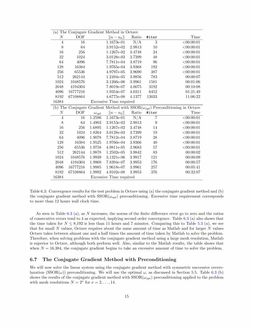
As seen in Table 6.3 (a), as N increases, the norms of the finite difference error go to zero and the ratiosof consecutive errors tend to 4 as expected, implying second order convergence. Table 6.3 (a) also shows thatthe time taken for N ≤ 8,192 is less than 11 hours and 7 minutes. Comparing this to Table 5.3 (a), we seethat for small N values, Octave requires about the same amount of time as Matlab and for larger N valuesOctave takes between almost one and a half times the amount of time taken by Matlab to solve the problem.Therefore, when solving problems with the conjugate gradient method using a large mesh resolution, Matlabis superior to Octave, although both perform well. Also, similar to the Matlab results, the table shows thatwhen N = 16,384, the conjugate gradient begins to take an excessive amount of time to solve the problem.

6.7 The Conjugate Gradient Method with Preconditioning

We will now solve the linear system using the conjugate gradient method with symmetric successive overre-laxation (SSOR(ω)) preconditioning. We will use the optimal ω, as discussed in Section 5.5. Table 6.3 (b)shows the results of the conjugate gradient method with SSOR(ωopt) preconditioning applied to the problemwith mesh resolutions N = 2ν for ν = 2, . . . , 14.

15

(a) (b)

Figure 6.2: The relative residual versus iteration number k for N = 32 for all iterative methods where “GS”represents Gauss-Seidel, “SOR” represents successive overrelaxation, “CG” represents conjugate gradient,and “PCG-SSOR” represents conjugate gradient with symmetric successive overrelaxation preconditioning.Figure (a) shows the graph to the maximum number of iterations required for all methods and (b) showsthe plot to k = 100. The black line represents the desired tolerance, 10−6. These figures were produced inOctave.

As seen in Table 6.3 (b), as N increases, the norms of the finite difference error go to zero and the ratiosof consecutive errors tend to 4 as expected. Table 6.3 (b) also shows that the time taken for N ≤ 8,192 isless than 33 minutes. Comparing this to Table 5.3 (b), we see that for all N values available in Table 6.3 (b),Octave requires about the same time to solve the problem as Matlab. However, Octave requires excessivetime to solve the problem when N = 16,384 regardless of whether it was run on a compute node with 64 GBof memory or an user node with 128 GB of memory, while Matlab could solve this mesh resolution in alittle over 3 hours on the user node. Therefore, when solving problems with the conjugate gradient methodwith symmetric successive overrelaxation (SSOR(ω)) preconditioning for a large mesh resolution, Matlab issuperior to Octave.

From the results in Tables 6.3 (a) and (b), we see that the conjugate gradient method with SSOR(ωopt)preconditioning converges with an order of magnitude fewer iterations and the time to reach convergencedecreases by a factor of ten. Therefore, we see the advantages of using a carefully selected preconditioningmatrix.

6.8 A Comparison of the Iterative Methods

To compare all iterative methods graphically, we will plot the relative residuals ||r(k)||2/||b||2 versus theiteration number k for N = 32 in a semi-log plot shown in Figure 6.2 (a) and (b). This plot is producedusing the semilogy command in Octave. Figures 6.2 (a) and (b) are clearly similar to Figures 5.2 (a) and (b)which were produced by Matlab. It is clear from Figure 6.2 (a) that the Jacobi and Gauss-Seidel methodstake far more iterations to converge than the remaining three iterative methods. It is clear from Figure 6.2 (b)that the conjugate gradient method with SSOR(ωopt) preconditioning is superior to the conjugate gradientmethod without preconditioning, which in turn is superior to SOR(ωopt).

16

7 Comparisons and Conclusions

We will now compare the methods discussed in Sections 5 and 6. We noted that Gaussian elimination wasmore efficient with sparse storage than dense storage. We saw that SOR(ωopt) was the most efficient of thethree classical iterative methods tested; however, it is slower than both Gaussian elimination and conjugategradients without being able to solve larger problems than these. We concluded that the conjugate gradientmethod with SSOR(ωopt) preconditioning was more efficient than the conjugate gradient method withoutpreconditioning. Therefore, we will compare now only Gaussian elimination with sparse storage and theconjugate gradient method with SSOR(ωopt) preconditioning.

Gaussian elimination with sparse storage in Matlab was able to solve the system for mesh resolutions upto N = 8,192 the fastest. Therefore, it is a good method to use for systems with sparse coefficient matricesand relatively small mesh sizes. However, for N = 16,384, this method runs out of memory. Gaussianelimination with sparse storage in Octave was only able to solve the problem for mesh resolutions up toN = 4,096, and ran out of memory when N = 8,192. For those mesh resolutions in which both Matlab andOctave were able to solve the problem, Octave was significantly slower with the highest N value. Thereforewhen solving a system using Gaussian elimination with sparse storage, Matlab should be used when a largevalue of N is needed.

The conjugate gradient method with SSOR(ωopt) preconditioning in Matlab is the best method for solvinga linear system for mesh resolutions larger than N = 8,192. This method did take longer than Gaussianelimination with sparse storage in Matlab for mesh resolutions N ≤ 8,192, however it was quicker than theSOR(ωopt) method. It was able to solve the system with a mesh resolution of N = 16,384 in Matlab in justover 3 hours. The conjugate gradient method with SSOR(ωopt) preconditioning in Octave was only able tosolve the problem for mesh resolutions up to N = 8,192. For those mesh resolutions in which Matlab andOctave were both able to solve the problem, Matlab and Octave required almost the same amount of time.Therefore, if one needs to solve a problem with a very large mesh resolution, the conjugate gradient methodwith SSOR(ωopt) preconditioning in Matlab should be used. Otherwise, if one needs to solve a problem usingthe conjugate gradient method with SSOR(ωopt) preconditioning for a smaller mesh size, both Matlab andOctave are good software choices.

Overall, it is important to consider the size of the mesh resolution used to determine which method andsoftware to use to solve the system. If the mesh resolution is very large, in this case N = 16,384, the onlymethod that will solve the problem is the conjugate gradient method with SSOR(ωopt) preconditioning inMatlab. If N ≤ 8,192, both Matlab and Octave can be used. If N = 8,192, Gaussian elimination with sparsestorage in Matlab will solve the problem the fastest. However, if Octave is used, the conjugate gradientmethod with SSOR(ωopt) preconditioning will solve the problem fastest without running out of memory. Forsmall N values, both Matlab and Octave can be used, and Gaussian elimination with sparse storage shouldbe used since it can solve the problem fastest.

We conclude that for problems of the textbook type typically assigned in a course, Octave would be asufficient software package. However, once one branches into more in-depth mathematics, Matlab should beused to provide faster results for problems.

We return now to the previous report on this test problem by comparing the timings on maya in thisreport with the timings on tara reported in [1]. Precisely, for the results on the conjugate gradient method,we compare Table 5.3 (a) here with Table 3.1 (b) in [1] for Matlab and Table 6.3 (a) here with Table 3.2 (b)in [1] for Octave. The timings for the conjugate gradient method on maya are twice as fast as those wereon tara in each case. For the results on Gaussian elimination with sparse storage, we compare Table 5.1 (b)here with Table 3.1 (a) in [1] for Matlab and Table 6.1 (b) here with Table 3.2 (a) in [1] for Octave. Gaussianelimination in Octave solved the same size of problem on maya as on tara before running out of memory; thespeed improved by a factor of about three in all cases. Gaussian elimination in Matlab was able to solve theproblem on a finer mesh on maya than on tara; the speed improved modestly, starting from already excellenttimings on tara in [1]. The speedup observed here for Matlab and Octave from tara to maya is consistentwith the speedup for serial jobs in the C programming language for this test problem reported in [5].

17

Acknowledgments

The hardware used in the computational studies is part of the UMBC High Performance Computing Facility(HPCF). The facility is supported by the U.S. National Science Foundation through the MRI program (grantnos. CNS–0821258 and CNS–1228778) and the SCREMS program (grant no. DMS–0821311), with additionalsubstantial support from the University of Maryland, Baltimore County (UMBC). See www.umbc.edu/hpcf

for more information on HPCF and the projects using its resources. This project began as the class projectof the first author for Math 630 Numerical Linear Algebra during the Spring 2014 semester [6]. The secondauthor acknowledges financial support as HPCF RA.

References

[1] Ecaterina Coman, Matthew W. Brewster, Sai K. Popuri, Andrew M. Raim, and Matthias K. Gobbert.A comparative evaluation of Matlab, Octave, FreeMat, Scilab, R, and IDL on tara. Technical Re-port HPCF–2012–15, UMBC High Performance Computing Facility, University of Maryland, BaltimoreCounty, 2012.

[2] James W. Demmel. Applied Numerical Linear Algebra. SIAM, 1997.

[3] Anne Greenbaum. Iterative Methods for Solving Linear Systems, vol. 17 of Frontiers in Applied Mathe-matics. SIAM, 1997.

[4] Arieh Iserles. A First Course in the Numerical Analysis of Differential Equations. Cambridge Texts inApplied Mathematics. Cambridge University Press, second edition, 2009.

[5] Samuel Khuvis and Matthias K. Gobbert. Parallel performance studies for an elliptic test problem on thecluster maya. Technical Report HPCF–2014–6, UMBC High Performance Computing Facility, Universityof Maryland, Baltimore County, 2014.

[6] Sarah Swatski. Solving the Poisson equation using several numerical methods, 2014. Department ofMathematics and Statistics, University of Maryland, Baltimore County.

[7] David S. Watkins. Fundamentals of Matrix Computations. Wiley, third edition, 2010.

[8] Shiming Yang and Matthias K. Gobbert. The optimal relaxation parameter for the SOR method appliedto the Poisson equation in any space dimensions. Appl. Math. Lett., vol. 22, pp. 325–331, 2009.

18