Embed Size (px)
Citation preview
Journal of Atmospherrc and Terrestrral Physics, Vol. 50, No. 9, pp. 763-780, 1988. OOZI-9169188 WOO+ 00
Printed in Great Britain. d: 1988 Pergamon Press plc
A comparison of northern and southern hemisphere TEC storm behaviour
J. E. TITHERIDGE and M. J. BUONSANTO*
Department of Physics, The University of Auckland, Private Bag, Auckland, New Zealand
(Received injinalform 4 March 1988)
Abstract-Changes in total electron content during magnetic storms are compared at stations with similar geographic and geomagnetic latitudes and eastward declinations in the northern and southern hemispheres.
Mean patterns are obtained from 58 storms at f 35” and 28 storms at 5 20” latitude. The positive storm phase is generally larger (and earlier) in the southern hemisphere, while negative storm effects are larger in the north. These changes reduce the normal asymmetry in TEC between the two hemispheres. Composition changes calculated from the MSIS86 atmospheric model agree well with the maximum decreases in TEC in both seasons (when changes in the F-layer height are ignored). Recovery occurs with a time constant of about 35 h; this is 50% longer than in the MSIS86 model. There is a marked diurnal variation at 35’S, with a rapid overnight decay and enhanced values of TEC in the afternoon. This pattern is inverted (and weaker) at 35”N, where night-time decay is consistently slower than on undisturbed nights. These results require a diurnal change in composition of opposite sign in the two hemispheres, or enhanced westward winds at night changing to eastward near sunrise. There is some evidence for both these mechanisms. Following a night-time sudden commencement there is a large annual effect with daytime TEC increasing for storms near the June solstice and decreasing near December. Storms occurring between November and April tend to give large, irregular increases in TEC for several days, particularly at low latitudes. In summer and winter at both stations, the mean size of the negative phase does not increase for storms with K, z 6. The size of the positive phase is proportional to the size of the change in ap in winter, while in summer a positive phase is seen only for the larger storms
1. INTRODUCTION
Although the response of the ionosphere to geo- magnetic storms has been studied for many years, there remain many longitudinal and hemispherical differences which are not well understood. In this paper we analyze storm behaviour as seen in total electron content (TEC) at two northern and two sou-
thern hemisphere stations, with similar geographic and geomagnetic conditions. Previous studies of storms at several stations have been carried out using bothfoF2 and TEC, but this is the first study specifi- cally designed to compare TEC storm behaviour in the two hemispheres.
MATSUSHITA (1959) studied storms in NmF2 at 38 stations over a ten year period. The mean storm time variation showed a short increase followed by a larger decrease at the higher latitudes, with little change at low latitudes. This average pattern was affected by season, with the decrease extending to lower latitudes in summer. The local time of maximum decrease was later at decreasing latitudes. Other studies of NmF2 changes at several stations are by RAJARAM and
*Present address : MIT Haystack Observatory, Westford, MA, U.S.A.
RASTOGI (1970), SPURLINC and JONES (1973) and KANE (1973, 1975). Results showed the great varia-
bility and the large longitudinal differences in storm behaviour. KOTADIA (1965) and KOTADIA and JANI (1967) showed that seasonal effects are much smaller at low latitudes.
Early studies of TEC behaviour during storms
(TITHERIDGE and ANDREWS, 1967 ; HIBBERD and Ross, 1967 ; GOODMAN, 1968 ; TAYLOR and EARNSHAW, 1969) showed that the total content behaved similarly to the peak density, except that the slab thickness ( = TEC/NmF2) generally increased, especially in the first few days of the storms. Case studies of the changes in TEC during very large storms, using data from a large number of stations, have been made by KLOBUCHAR et al. (1971), SCHODEL et al. (1974) and ESSEX et al. (1981). TANAKA (1979) studied the changes in foF2 at 41 stations. The importance of the local time of storm commencement and the seasonal differences in TEC variations, were shown by all these case studies.
Using TEC data from Hamilton, Massachusetts, MENDILLO (1971) and HARGREAVES and BAGENAL (1977) calculated mean TEC storm behaviour accord- ing to both local time and storm time (time from the sudden or gradual magnetic storm commencement).
163
164 J. E. TITHERIDGE and M. J. BUONSANTO
Behaviour at Goose Bay, Labrador (L = 4) was com- pared with the Hamilton results by BUONSANTO et al. (1979). This and other work (MENDILLO et al., 1974; MENDILLO and KLOBUCHAR, 1975 ; MENDILLO, 1978) showed the importance of trough dynamics in pro- ducing a negative phase which begins progressively later at sites with lower latitudes.
The most comprehensive experimental study of TEC storm behaviour was presented by M~DILLO (1978), who calculated the average behaviour for a large number of storms at 8 stations. Seasonal differ- ences were also examined where possible. Five of the stations are located in eastern North America, at invariant latitudes of 41”63” and 3 stations (in Greece, Korea and Rhodesia) have invariant latitudes of 27”N, 31”N and 30”s. The importance of trough dynamics was clearly demonstrated in the TEC behav- iour at stations along the latitude chain. Differences were found between the TEC behaviour at the three low latitude stations but mainly increases occurred.
TEC during storms at Arecibo was discussed by NELSON and COGGER (1971) and compared with TEC at Hamilton by LANZEROTTI et al., 1975). TEC gen- erally increased at Arecibo while both increases and decreases were found at Hamilton. TEC and NmF2 data from four very severe storms in the East Asian zone, observed at dip latitudes of 21”N-26”N, have been presented by TIAN-XI (1985). The summer storms showed depletions irrespective of storm com- mencement time and local time.
Of special interest to this work, RAJARAM and RASTOGI (1970) presented NmF2 data from the Maui/ Rarotonga pair of stations. Changes in NmF2 were somewhat more negative at Maui in summer and for the year as a whole.
HUANG et al. (1974) and BASU et al. (1975) described TEC storm variations at Honolulu. MEN- DILLO (1976) calculated TEC local time storm vari- ations at Stanford. JONES (1971) compared TEC at Auckland and NmF2 at Auckland, Norfolk Island (29”S, 16X”E) and Munda~ng (32’S, 116”E). Longi- tudinal differences were interpreted in terms of an asymmetrical local time distribution of storm com- mencements. It has been shown, however, that this longitudinal difference in ionospheric behaviour is closely related to a longidutinal difference in O/N, sto~time changes (Pnij~ss and VON ZAHN, 1974 ; Priilss et at., 1975 ; TRINKS ei af., 1975). Pnfi~ss (1980) reviewed results of satellite measurements of thermospheric density perturbations and their close relationship with NmF2 during storms. MILLER et al. (1984) found a direct correlation between topside electron density and the O/N, ratio during one geo- magnetic storm. Theoretical studies (eg. VOLLAND,
1979; RISHBETH et al., 1985) are also beginning to provide an understanding of the thermospheric storm and allied ionospheric effects.
2. PRESENT UNDERSTANDING
2.1. The positive phase
An ionospheric storm is an extremely complex phenomenon. Changes in the production, loss and movement of ionisation are caused by various factors which depend upon location (latitude, longitude and altitude), season, geomagnetic storm commencement time and local time.
With the onset of the geomagnetic storm, Joule heating due to electric currents (COLE, 1971; MAYR and VOLLAND, 1974) and heating caused by particle precipitation, causes an increase in the atmospheric pressure at high latitudes. This produces gravity waves and causes or enhances an equatorward neutral wind at F-region heights (VOLLAND, 1979 ; BLANC and RICHMOND, 1980; RILLEEN and ROBLE, 1986). Shifts of neutral winds to equatorward (SIPLER and BIONDI, 1979) and enhanced equatorward winds (HERNANDEZ and ROBLE, 1976) have been observed from air- glow observations at night and deduced from in- coherent scatter drift measurements during the day (~AZAUDIER and BERNARD, 1985). These winds will lift the ionisation to regions of lower loss, producing daytime increases in hmF2 (SPURLING and JONES, 1976), in foF2 and in TEC (JONES and RISHBETH, 1971; JONES, 1973).
East-west ionisation drifts during storms may also be important. These drifts of ionisation will be west- ward in the dusk sector and eastward in the dawn sector (e.g. MENDILLO, 1973). By ion drag they might cause westward neutral winds in the evening and east- ward ones in the early morning, opposite to the normai pattern, as observed by YAGI and DYSON (1985a,b). Their possible role in producing observed TEC storm variations is discussed in Section 7.3.
At high and mid-latitudes, the positive phase is restricted to the early stages of a storm. It is limited to the dusk sector in Hamilton TEC (MENDILLO et al., 1970; PAPAGIANNIS et al., 1971) and in Millstone Hill TEC and NmF2 (EVANS, 1970) and coincides with increases in total geomagnetic field intensity. This suggests that enhanced E x B vertical drifts due to magnetospheric convection electric fields, which will be upward during the day, may also be involved in producing the TEC positive phase (EVANS, 1970; MENDILLO, 1975). Theoretical studies (STUBBE and CHANDRA, 1970; DAVIES and RUSTER, 1976) have concluded that both winds and electric fields may be

Northern and southern hemisphere TEC storm behaviour 165
important. An eastward electric field will produce not
only an upward drift but also a poleward one. The poleward drift eventually gives a poleward neutral
wind, such that the ionisation moves horizontally at
a fixed height. This ‘feedback effect’ occurs with a time constant of approximately 1 h (MATUURA, 1972), so electric fields may have only a short-term role in the initial positive phase.
At low latitudes atomic oxygen density is enhanced by a transport from higher latitudes (e.g. VOLLAND,
1979) and/or by a downward flow that balances the upwelling in the aurora1 oval (RISHBETH et al., 1985). This combines with the increase in hmF2 caused by equatorward winds to give prolonged enhancements in F-region electron densities.
2.2. The negative phase
The response time for winds or electric fields to lift the ionisation and produce the initial positive phase of a storm is quite short. The negative phase which
often follows takes longer to develop. SEATON (1956) first suggested that neutral composition changes could cause the decrease in foF2 observed during iono- spheric storms, and this was confirmed theoretically
by JUNG and PR~~LSS (1978). DUNCAN (1969) sug- gested that the thermospheric circulation would be
modified during storms and a number of papers have been published (CHANDRA and SPENCER, 1976 ; NISBET et al., 1977; MAYR and HEDIN, 1977; POTTER et al.,
1979; HEDIN et al., 1981 ; MILLER et al., 1984; PR~~LSS, 1987) giving evidence of composition changes which support this idea. Changes in thermospheric cir- culation and wind-induced diffusion of the neutral constituents act to decrease O/N2 and O/O, at middle and high latitudes and to increase these ratios or keep them fairly constant at low latitudes (e.g. MAYR and
VOLLAND, 1973). Other possible mechanisms for pro- ducing changes in composition are increased atmo-
spheric mixing due to gravity waves (KING, 1971), increased eddy diffusion (CHANDRA and SINHA, 1974)) or particle heating (RISHBETH et al., 1985).
During quiet times the neutral winds blow primarily from the summer to the winter hemisphere (BLUM and HARRIS, 1975; DICKINSON, et al., 1981). During storms the enhanced equatorward winds will oppose the summer to winter circulation in the winter hemi- sphere, but add to it in the summer hemisphere. Thus, the area of enhanced N2/0 extends to lower latitudes in summer and sharp latitudinal gradients of N,/O occur in winter (PR~LSS and VON ZAHN, 1977). This accounts for the confinement of negative storm effects to higher latitudes in winter than in summer (PR~~Lss, 1977).
3. DATA AND METHOD OF ANALYSIS
The TEC data used in this study were discussed in an earlier paper (TITHERIDGE and BUONSANTO, 1983)
which dealt with annual variations in TEC at the same
four stations. Table 1 gives the coordinates of the stations and the periods studied. The Raratonga- Honolulu stations are nearly magnetically conjugate. Both pairs of stations have nearly the same geographic latitudes (north and south of the equator), the same geomagnetic dip latitudes and the same magnetic declination.
Magnetic storms considered in the present work
were selected according to the following criteria. The planetary index K, must be 5 or more for at least two 3 h periods. The magnetic disturbance must be followed by at least 3 days of relative quiet, so that the post storm recovery can be seen. The duration of the disturbance must be less than 48 h, so that the initial and main phases of the ionospheric response will not overlap too much. Large storms with mag- netic activity continuing for several days have not been included in the mean plots, since they give large, irregular fluctuations in TEC, which tend to mask the
pattern obtained from more clearly defined storms. Results for any storm are terminated before the onset of a following storm, so that renewed activity does not hide the normal storm recovery pattern. Thus, in many plots the number of storms averaged at day 5 is less than the number for days 14.
TEC data were available from December 1967 through to December 1971 for part or all of 58 storm periods at Stanford, and 57 storm periods at Auckland. A subset of this number is used to obtain
storm patterns for Honolulu and Raratonga (28
storms) for the period June 197GDecember 1971. Table 2 lists the storms analysed. The table gives the
dates of the storm commencements, the sudden storm
commencement times (if observed) at Honolulu
and/or Apia (two stations in the same longitude zone),
the maximum K, value during the storm, the type of storm (D for ‘December type’, J for ‘June type’) and
the stations at which data were available for part or all of each storm period.
For most plots the data are divided into two
seasons : ‘June’ : April-September and ‘December’ : October-March. Use of more seasons would con- siderably increase the number of plots and decrease the number of storms included in each average. Exam- ination of individual results showed that storms near equinox appeared to be of either the June or December type, with no distinct equinox pattern. Thus, the
storms on 5 April 1968 and 3 April 1971 are of the December type and storms on 2 and 12 October 1968
166 J. E. TITHERIDGE and M. J. BUONSANTO
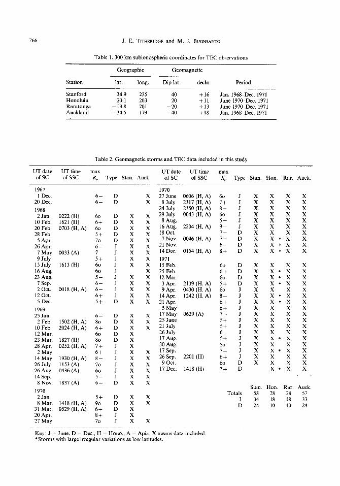
Table I. 300 km subionospheric coordinates for TEC observations
Station
Geographic Geomagnetic
lat. long. Dip lat. decln. Period
Stanford 34.9 235 40 +I6 Jan. 196%Dec. 1971 Honolulu 20.1 203 20 +11 June 197&Dec 1971 Raratonga -19.8 201 -20 f13 June 1970-Dec. 1971 Auckland -34.5 179 -40 +I8 Jan. 1968-Dec. 1971
Table 2. Geomagnetic storms and TEC data included in this study
UT date UT time max UT date UT time max of SC of SSC K, Type Stan. Auck. of SC of ssc Kp
1967 1 Dec.
20 Dec.
1968 2 Jan.
10 Feb. 20 Feb. 28 Feb.
5 Apr. 26 Apr.
7 May 9 July
13 July 16 Aug. 23 Aug.
7 Sep. 2 Oct.
12 Oct. 5 Dec.
1969 25 Jan.
2 Feb. 10 Feb. 12 Mar. 23 Mar. 28 Apr.
2 May 14 May 26 July 26 Aug. 14 Sep. 8 Nov.
1970 2 Jan. 8 Mar.
31 Mar. 20 Apr. 27 May
6- 6-
0222 (H) 60 1621 (H) 6+ 0703 (H, A) 60
5+ 70
6- 0033 (A) 7-
5+ 1613 (H) 60
60 5- 6-
0018 (H, A) 6- 6+ 5+
6- 1502 (H, A) 80 2024 (H, A) 6+
60 1827 (H) 80 0252 (H, A) 7f
6+ 1930 (H, A) 8- 1153 (A) 70 0436 (A) 60
5- 1837 (A) 6-
1418 (H, A) 9’: 0529 (H, A) 6+
8+ 70
D D
D D D D D J J J J J J J J J D
D D D D D J J J J J J D
D D D J J
X X X X X X X X X
X X X X X
X X X X X X X X X X X X
X X X X X
X X
X X X X X X X X X X X X X X X
X X X
X X X X X X
X X
X
1970 27 June
8 July 24 July 29 July
8 Aug. 16 Aug. 18 Oct. 7 Nov.
21 Nov. 14 Dec.
1971 15 Feb. 25 Feb. 12 Mar. 3 Apr. 9 Apr.
14 Apr. 21 Apr.
5 May 17 May 25 June 21 July 26 July 17 Aug. 30 Aug. 17 Sep. 26 Sep.
9 Oct. 17 Dec.
0606 (H, A) 2317 (H, A) 2350 (H, A) 0043 (H, A)
2204 (H, A)
0046 (H, A)
0154 (H, A)
2139 (H, A) 0430 (H, A) 1242 (H, A)
0629 (A)
2201 (H)
1418 (H)
60 7+ 8- 60 5+ 9- 7- 7- 6- 8+
60 6+ 60 5+ 60 8- 6-1 6+ 7- 5+ 5+ 6- 5+ 50 7- 6+ 60 7+
Type Stan. Hon. Rar. Auck.
J J J J J J D D D D
D D D D J J J J J J J J J J J J D D
X X X X X X X X X X
X X X X X X X X X X X X X X X X X
x x x x x x x x x x x x x x x*x x*x x * x
x x x*x x*x x*x x x x*x x*x x x x x x x x x x x x* x x x x* x x x x x x* x
X X X X X X X X X X
X X X X X X X X X X X X X X X X X X
Totals J D
Stan Hon. Rar Auck. 58 28 28 57 34 18 18 33 24 10 10 24
Key : J = June, D = Dec., H = Hono., A = Apia. X means data included. *Storms with large irregular variations at low latitudes.

Northern and southern hemisphere TEC storm behaviour 161
follow the June pattern. This agrees with other obser-
vations which indicate that the change from ‘summer’
to ‘winter’ conditions in the ionosphere commonly occurs about two weeks after the equinoxes.
Hourly data are used throughout, adjusted to the correct local solar time. For all local time plots differ- ent storm periods are combined by placing the main peak of magnetic activity in day 1. This is done regard- less of the time of any sudden commencement since, as discussed in Section 4, the presence or absence of
a sudden commencement does not seem to be of
importance in determining the ionospheric changes. For a given UT the local solar times differ by 4 h at Auckland and Stanford. Thus, about one sixth of the storms are placed in different days for these two stations. If this adjustment is not done then the Stan- ford plots have appreciably higher mean activity on the morning of day 2, leading to some anomalies in the comparison with Auckland data.
To determine the changes caused by magnetic activity other workers have used simple control curves such as the monthly median, the monthly mean, seven days before the storm, or simply one quiet day during the same month. The control curves used in the pre- sent work are designed to give an improved rep-
resentation of the ‘quiet’ ionosphere. They are defined by mean hourly values for 20 days before and 20 days after the storm period, including only those values for
which K, < 4 and the average of Kp over the previous 72 h was less than 3. The first condition (Kp < 4) elim- inates very disturbed periods from the control curve. The second condition omits data corresponding to the aftermath of geomagnetic storms, when the iono- sphere is still recovering. With these conditions the control curves are generally an average of about 3& 35 values at each hour ; in only one case is the number averaged less than 20.
The quiet day data were also used to obtain vari- ations for one standard deviation above and below the control curve for each storm. These results were averaged to give the variations plotted as dotted lines in some figures. For per cent deviation plots the dotted lines are an average over both hemispheres, since the quiet time variability (expressed as a percentage of the mean value) is much the same in both hemispheres. For one storm, a TEC variation which reached the dotted lines would have a significance level of only about 68%. For the average over many storms sig- nificance levels are much higher. In Figs. 1 and 6, variations which reach half way to the dotted lines have a statistical significance exceeding 99%.
Figures showing the per cent deviation of TEC have been smoothed by the application of a digital filter using weights 1, 4, 6, 4, 1. This removes rapid (hour
I . I . I . I .
Day1 ’ Day2 ’ Day3 ’ Doyl - Day5 Local Tame
Fig. 1. Mean values of TEC, averaged over all storms and all seasons, for Stanford (35”N, 58 storms) and for Auckland (35”S, 57 storms). The lower curves (b) show the percentage deviation from the quiet-time reference curve. Changes in the 3 h a,, index, averaged over all storms, are shown at the top of the figure. Dotted lines correspond to one standard deviation above and below the mean for the quiet day vari-
ations.
to hour) fluctuations from the data. Curves at the top of each figure give the mean of the 3 h up indices.
These curves are shown separately for the northern hemisphere (continuous lines) and the southern hemi- sphere (broken lines) when the selection of different storms for the two hemispheres gives an appreciable
difference in the mean activity.
4. MID-LATITUDE RESULTS
4.1. Local time variations
The mean variation of TEC for the mid-latitude
stations, averaged over all storms, is shown in Fig. l(a). Dotted lines give the range (to f 1 standard deviation) covered by the normal day-to-day varia- bility of the ‘quiet’ ionosphere. These plots show clearly higher values of TEC at 35”N than at 35”s during the day, for quiet and disturbed conditions. This effect is due primarily to composition changes, which produce an increase of 80% in the northern

768 J. E. TITHERIDGE and M. J. BUONSANTO
TEC from October to April, and to the effect of neutral winds (TITHERIDGE and BUONSANTO, 1983).
Figure l(b) shows the changes in TEC, caused by magnetic activity, expressed as a percentage of the mean quiet-day values. In both hemispheres TEC increases considerably on the first day of the storm, decreases rapidly after local midnight and remains low for several days. Compared with the northern hemisphere results, changes at 35”s show: (1) a doubled increase by noon on the first day ; (2) a faster overnight decay, giving a sharp minimum near sunrise at all stages of the storm ; (3) increased values of TEC, from about 1000 to 2200 LT, on all disturbed days. This last effect leads to a greater positive phase and a smaller negative phase, in the southern hemisphere.
At both stations the storm recovery is completed by about the end of day 5. On days 14 the TEC deviations are generally more positive (or less nega- tive) at 35”s. The difference is due primarily to the consistent diurnal variation at 35”S, with increased values during the day and a more rapid overnight decay. This behaviour is the reverse of the normal quiet day variations when, compared to 35”N, TEC at 35”s is lower during the day and higher at night. Thus, storm effects tend to reduce the ‘normal’ differ- ence in TEC between the two hemispheres.
The above features are present to some extent in all seasons. This is shown in Fig. 2, where results are presented separately for the summer and winter groups. The summer variation is reasonably smooth with a peak increase of about 10% on the evening of day 1, followed by a rapid decrease to a minimum of about -20% from sunrise to sunset on day 2. This is followed by a steady recovery which is completed by the end of day 5.
The mean winter response (Fig. 2b) shows con- siderable differences from the summer pattern. The positive phase is more than twice as large, exceeding 25% on the evening of day 1. The following decrease is more gradual, extending from roughly 2200 on day 1 to 2200 on day 2. Thus the negative phase is not fully established at both stations until the beginning of day 3. The decrease of about 8% at this time is only half as large as in summer. Recovery is slower in winter so that the mean decrease on day 4 is about the same in both seasons.
In both winter and summer the southern hemi- sphere storms are more positive (or less negative) near noon, throughout the storm period. This daytime increase appreciably reduces the magnitude of the negative phase in summer. In winter the southern hemisphere curves show a rapid night-time decay of ionisation. Combined with the daytime enhancement this gives a very marked diurnal variation, with sharp
i (a) SUMMER
lb) WINTER
V, I I 1 10~2 ’ Day3 ’ DayL ’ Day5
Local Time
Fig. 2. Mean percentage deviations of TEC at mid-latitudes. Summer results (a) include 34 storms at 35”N and 24 storms at 35”s. Winter results (b) are from 24 storms at 35”N and 33 storms at 35”s. Dotted lines show the variations expected from a fixed increase in the loss coefficient at night (Section
7.1.2.).
minima at sunrise and broad maxima shortly after
noon. For the northern hemisphere, the solid curve in Fig. 2(b) shows maximum values near sunrise and minima near sunset. Thus from day 1 to day 4 the winter responses show large diurnal variations, par- ticularly in the southern hemisphere, and these are of opposite phase in the two hemispheres.
4.2. Changes with storm size
Storm patterns also depend to some extent on the size of the magnetic disturbance. To show this, all storms in Table 2 were classified as ‘small’ or ‘large’ on the basis of the 4 largest values of the 3 h index a,,. Eleven storms of intermediate size were omitted to give a clearer separation between the two groups. The maximum value of Kp is greater than 6+ for most of the large storms and < 6- for the small group. As shown by the separate up curves in Fig. 3, the mean storm time increase in up (above the refer- ence value, indicated by a horizontal line) is about twice as large for the ‘large’ storms as for the ‘small’ group.
In summer (Fig. 3a,b) the positive phase cor-

Northern and southern hemisphere TEC storm behaviour 169
Id1 WINTER
39s.
I a ! 1 [ 8 ! 11 8 [ 5 ! 2 ! a I Day 1 clay 2 Day 3 Day& Day 1 Day2 Day 3 Day L
Local Time
Fig. 3. The effect of storm size on the ionospheric response at latitudes of k 35”. Solid and broken lines are for storms with maximum K, values of > 6 - and < 6 +, respectively. The number of storms in each
group is shown by the corresponding a, plot.
responds to an increase of about 15% for the large storms, but only about 3% for the small group. Thus, a doubling of the mean increase in ap gives an increase of roughly 5 times in the size of the positive phase, at
both stations. The large negative phase is, however, almost the same for both groups. The storms in Fig. 3a are quite separate from those in Fig. 3b. The simi- larity of the patterns in these two figures indicates that this unequal dependency of the positive and negative effects on storm size is a real effect.
In winter (Fig. 3c,d) there is a large positive phase under all conditions, with an increase in TEC roughly
proportional to the mean increase in up. The size of the negative phase is, however, almost independent of the size of the disturbance, for both stations and both seasons. Thus, in summer the large negative phase increases by a factor of less than 1.3 when the changes in up are doubled. In winter the mean negative phase is, if anything, slightly less for the larger storms. This may indicate that larger storms carry the same com- position changes to lower latitudes, or that further increases in N2 density are offset by a spread of the
low latitude enhancements of atomic oxygen (MILLER
et al., 1984) to higher latitudes. The dominant diurnal variations, at 35”S, are most
marked for the large winter disturbances in Fig. 3d.
These produce a major increase in TEC throughout the day, maximising in the late afternoon, followed
by a rapid decay from sunset to sunrise. Similar variations are not apparent in any of the northern hemisphere results. Possible causes for this effect are considered in Section 7 below.
4.3. Dependence on storm time
Observed storm effects may depend on the occur- rence of a sudden storm commencement (s.c.) and the time of the S.C. Of the 62 storms considered in this study, 29 had a S.C. recorded at Hawaii or Apia stations near the geographical centre of the observing region. Plotted storm responses showed appreciable differences for groups with and without a S.C. These were, however, due primarily to differences in the size of the magnetic disturbances. The S.C. group included 8 of the 9 largest storms and only 1 of the 12 smallest.
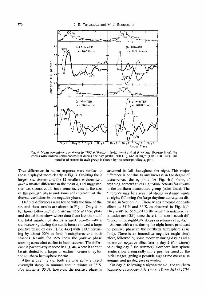
770 J. E. TITHERIDGE and M. J. BUONSANTO
Ic) WINTER
SC. DAY 106.18,
Local Time
Fig. 4. Mean percentage deviations in TEC at Stanford (solid lines) and at Auckland (broken lines), for storms with sudden commencements during the day (060~1800 LT), and at night (1800-0600 LT). The
number of storms in each group is shown by the corresponding aP plot.
Thus differences in storm response were similar to those displayed more clearly in Fig. 3. Omitting the 9 largest S.C. storms and the 12 smallest without s.c., gave a smaller difference in the mean up and suggested that S.C. storms could have some increase in the size of the positive phase and some enhancement of the diurnal variations in the negative phase.
Definite differences were found with the time of the S.C. and these results are shown in Fig. 4. Only data for hours following the S.C. are included in these plots and dotted lines show where data from less than half the total number of storms is used. Storms with a S.C. occurring during the sunlit hours showed a large positive phase on day 1 (Fig. 4a,c) with TEC increas- ing by about 30% in both hemispheres and both seasons. Results for 35”s show the positive phase starting somewhat earlier in both seasons, The differ- ence is particularly marked in Fig. 4a, where it cannot be attributed to a larger or earlier increase in ap for the southern hemisphere storms.
After a daytime S.C. both stations show a rapid overnight decay in summer and in winter at 35”s. For winter at 35”N, however, the positive phase is
sustained in full throughout the night. This major difference is not due to any increase in the degree of disturbance; the aP plots for Fig. 4(c) show, if anything, somewhat less night-time activity for storms in the northern hemisphere group (solid lines). The difference may be a result of strong westward winds at night, following the large daytime activity, as dis- cussed in Section 7.3. These winds produce opposite effects at 35”N and 35”S, as observed in Fig. 4(c). They must be confined to the winter hemisphere (at latitudes near 35”) since there is no north-south dif- ference in the night-time decays in summer (Fig. 4a).
Storms with a S.C. during the night hours produced no positive phase in the northern hemisphere (Fig. 4b,d). There is an immediate negative (night-time) effect, followed by some recovery during day 2 and a maximum negative effect late in day 2 (for winter) or during day 3 (in summer). Southern hemisphere results show a markedly more positive trend in the initial stages, giving a possible night-time increase in summer and no decrease in winter.
On day 2, following a night-time s.c., the southern hemisphere response differs totally from that at 35”N.
Northern and southern hemisphere TEC storm behaviour 771
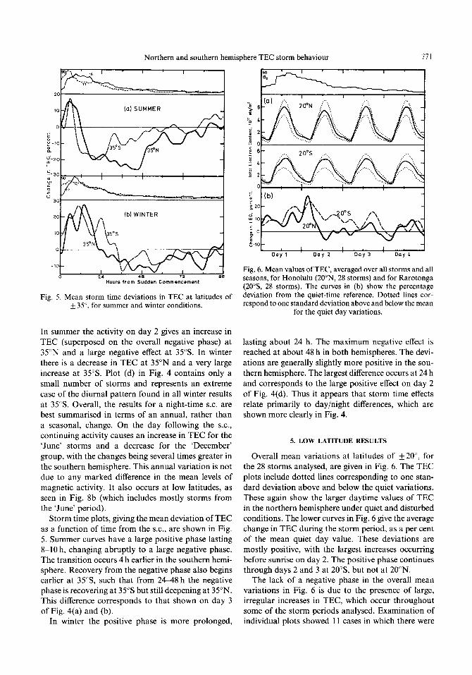
(al SUMMER
Hours from Sudden Commencement
Fig. 5. Mean storm time deviations in TEC at latitudes of + 35”. for summer and winter conditions.
In summer the activity on day 2 gives an increase in TEC (superposed on the overall negative phase) at 35”N and a large negative effect at 35% In winter there is a decrease in TEC at 35”N and a very large increase at 35%. Plot (d) in Fig. 4 contains only a
small number of storms and represents an extreme case of the diurnal pattern found in all winter results at 35% Overall, the results for a night-time S.C. are best summarised in terms of an annual, rather than a seasonal, change. On the day following the s.c., continuing activity causes an increase in TEC for the ‘June’ storms and a decrease for the ‘December’ group, with the changes being several times greater in
the southern hemisphere. This annual variation is not due to any marked difference in the mean levels of magnetic activity. It also occurs at low latitudes, as seen in Fig. 8b (which includes mostly storms from the ‘June’ period).
Storm time plots, giving the mean deviation of TEC as a function of time from the s.c., are shown in Fig. 5. Summer curves have a large positive phase lasting 8-10 h, changing abruptly to a large negative phase. The transition occurs 4 h earlier in the southern hemi- sphere. Recovery from the negative phase also begins earlier at 35”S, such that from 24-48 h the negative phase is recovering at 35”s but still deepening at 35”N. This difference corresponds to that shown on day 3 of Fig. 4(a) and (b).
In winter the positive phase is more prolonged,
I I I
Day1 ’ Day2 ’ Day3 ’ Day L 1
Fig. 6. Mean values of TEC, averaged over all storms and all seasons, for Honolulu (20”N, 28 storms) and for Rarotonga (2O”S, 28 storms). The curves in (b) show the percentage deviation from the quiet-time reference. Dotted lines cor- respond to one standard deviation above and below the mean
for the quiet day variations.
lasting about 24 h. The maximum negative effect is
reached at about 48 h in both hemispheres. The devi- ations are generally slightly more positive in the sou- thern hemisphere. The largest difference occurs at 24 h and corresponds to the large positive effect on day 2
of Fig. 4(d). Thus it appears that storm time effects relate primarily to day/night differences, which are shown more clearly in Fig. 4.
5. LOW LATITUDE RESULTS
Overall mean variations at latitudes of *20”, for the 28 storms analysed, are given in Fig. 6. The TEC
plots include dotted lines corresponding to one stan- dard deviation above and below the quiet variations. These again show the larger daytime values of TEC in the northern hemisphere under quiet and disturbed conditions. The lower curves in Fig. 6 give the average
change in TEC during the storm period, as a per cent of the mean quiet day value. These deviations are mostly positive, with the largest increases occurring before sunrise on day 2. The positive phase continues through days 2 and 3 at 2O”S, but not at 20”N.
The lack of a negative phase in the overall mean variations in Fig. 6 is due to the presence of large, irregular increases in TEC, which occur throughout some of the storm periods analysed. Examination of individual plots showed 11 cases in which there were

J. E. TITHERIDGE and M. J. BUONSANTO 712
40
20
0
-20
Local Time
Fig. 7. Mean percentage deviations of TEC at latitudes of 20”N (solid lines) and 203 (broken lines). Results (a) are for storms showing large, irregular increases in TEC (exceeding
100% after day 2).
large increases in TEC (by more than 100% at one
station and more than 60% at both stations) occurring after the first 2 days of the storm interval. These events are unlike anything observed at higher latitudes, where increases never exceeded 80% at either station
after the first 2 days. The storms concerned are marked with an asterisk in Table 2 and show no clear
dependence on season or on the occurrence of a sud- den commencement. There is however an annual vari- ation. The six month period from May to October had 17 storms (at latitudes of +20”) with only 2 irregular, while in the six months from November to April there were 11 storms with 9 irregular. An exam- ple of the irregular variations is shown in Fig. 10, where TEC increases, on the third day of the storm, reach 200% at 20”s.
The mean TEC deviations for the 11 ‘irregular’ storms are shown in Fig. 7(a). Averaging over both hemispheres, and digitally filtering the result to remove short period variations, gives the fine line which indicates a sustained increase of 2&25% for nearly 4 days. Superimposed on this the results for
20”s show consistent peaks in the late afternoon, with minima before sunrise. This pattern agrees with the common diurnal variations at 35”S. The large vari-
ations at 20”N show no consistent L.T. pattern, but have an apparent periodicity of about 20 h. Many individual storms at 20”N show recurrent large peaks shortly before midnight. The 11 ‘irregular’ storms also show a clear tendency to produce unexpectedly large increases in TEC at latitudes of f 35”, throughout the 5 day storm period. The mean values of up, shown at the top of Fig. 7a, are not significantly larger for this group than for the other storms (in Figs. 7b,c).
The more regular storms were sorted by month,
rather than by season, since individual storms generally gave similar variations at both stations. The small ‘December’ group (Fig. 7b) shows this high correlation between the variations at 20”N and 20”s. At both stations there is a large positive phase, lasting
for about 24 h, followed by a smaller negative phase persisting for about 3 days. This negative phase dis- appears if the ‘irregular’ storms are included, since 7
of these are in the December interval. The mean variations from the June group (Fig. 7c)
show a short lived positive phase on the morning of day 2. This is much larger at 2O”S, where the onset of the negative phase is also more gradual. Thus, as at latitudes of f35”, deviations are consistently more positive (or less negative) in the southern hemisphere. The curves of Fig. 7(b) and (c) show no trace of the sunrise minimum and the afternoon maximum, which was commonly observed at 35”s and is seen at 20”s for the irregular storms.
Mean deviations for all storms with a sudden com- mencement occurring during the day (0600-1800 LT) and at night (1800-0600), are shown in Figs. S(a) and (b). In all cases there is an initial positive phase, increasing throughout the evening to a maximum shortly after midnight. At 20”N this is followed by a negative phase on day 2. At 20”s day 2 is approxi- mately normal after a daytime s.c., but shows a large positive effect after a night-time S.C. Four of the five storms included in Fig. 8(b) correspond to winter conditions in the southern hemisphere and the large daytime increase on day 2 is similar to that observed in winter at 35”s (Fig. 4).
Storm time plots are shown in Fig. 9. At 20”s the
deviations are generally positive in both seasons, while at 20”N there is a definite negative phase in summer. The positive phase lasts for about 18 h from the time of the S.C. Both stations show a large increase in winter, with a maximum at 12 h after the S.C. This appears to be a true seasonal effect. Other features at this latitude display annual differences, partly because of the great variability in the storm effects. Thus the

Northern and southern hemisphere TEC storm behaviour
la) DAY S.C.
10600-18001
(bl NIGHT S.C.
-201 ’ ’ 0 I I I I Day1 ’ Day 2 ’ Day 3 ’ DayL
Local Time
Fig. 8. Mean percentage deviations in TEC at Honolulu and Rarotonga, for storms commencing during the periods (a) 060&1800 LT and (b) 180&0600 LT. Curves (a) are an average over 8 storms (5 near June and 3 near December) while curves (b) include 5 storms (4 June and 1 December).
4 December storms give similar variations at both 20”s (a) and 20”N (b).
6. STORM VARIABILITY
Individual storms can show considerable variations from the mean patterns described above. Two rep- resentative examples are shown in Figs. 10 and 11,
using data from all four stations. On 14 April 1971 (Fig. 10) there is a period of high activity, with Kp reaching 8 -, for only a few hours near local noon. This produces a large positive phase at all stations, with TEC increasing to about 2.5 times the quiet day value. Similar large increases appear at irregular inter- vals for several days at the low latitude stations. The large increases on day 3 put this storm into the ‘irre- gular’ category of Fig. 7(a). There are no obvious features in the up plot to explain these increases, which occur simultaneously at most stations.
Figure 11 gives results for a storm of only moderate size (Kp = 60). Peak activity is at or before local sunset at the 3 southernmost stations, giving a marked increase in TEC. At 35”N the maximum activity
0 24 46 72 96 Hours from Sudden Commencement
Fig. 9. Mean storm time deviations in TEC for summer and winter conditions at latitudes of 20”N (solid lines) and 20”s
(broken lines).
Day of Month IL.T at 16O’WI
Fig. 10. Per cent deviations in TEC, as a function of local time, for the storm of 14 April 1971.
occurs about 2 h after sunset and there is no positive phase. A strong negative phase, lasting for several days, is seen at all stations (except 35”N, where all changes are small). The increases near sunset on 11 October show the quite large storm type response

J. E. TITHERIDGE and M. J. BUONSANTO
I I I I 8 9 ’ 10 ’ 11 ’ 12
Day of Month 1L.T. at 16O’W.l
Fig. Il. Per cent deviations in TEC, as a function of local time, for the storm of 9 October 1971.
which sometimes apppears with only moderate fluc- tuations in magnetic activity.
Both figures indicate strong hour-to-hour cor- relations in the TEC variations at 20”N and 2O”S,
during the main storm period and the following quiet interval. This correlation commonly extends to 35”N, and less commonly to 35”s. Overall variations are quite similar at all stations except for day 2 in Fig. 10, where 35”s shows the sunrise minimum and afternoon maximum which are typical of storm recovery at this station.
7. DISCUSSION
7.1. North-south d@erences at mid-latitudes
The storm responses at 35”N and 35”s show the same basic pattern, with an initial positive phase
(larger in winter) followed by a negative phase (larger in summer) and a recovery in about 5 days. There are, however, several clear differences. The most marked of these is a well defined diurnal variation in the storm response at 35”s. The effect is largest in winter (Figs. 2b and 3d), where the southern hemisphere results show a sharp minimum near sunrise and a broad maximum in the afternoon. At 35”N there is no trace of this diurnal pattern ; rather there is some opposite tendency with lower values of TEC in the afternoon and increased values near sunrise. Production of the diurnal variation at 35”s appears to involve two sep- arate effects, as discussed below.
1.1.1. Daytime enhancements. Compared with the
storm changes at 35”N, results for 35”s show an increased value of TEC from about 1000 to 2200 LT. In the overall mean plot (Fig. lb) this effect doubles
the size of the positive phase near noon on day 1
and almost eliminates the negative effect after noon on days 2-4. The effect is least in summer, when it shows no clear dependence on storm size. It is of major importance for the large winter storms, where it dominates all other effects at 35”s (Fig. 3d).
In a previous paper (TITHERIDGE and BUONSANTO,
1983) we compared the daytime equilibrium values of TEC at Auckland and at Stanford. This showed
an enhancement of about 80% at 35”N, from mid- October to mid-April. The difference was fully
explained by changes in atmospheric composition, as obtained from the MSIS model. The present results
show that, for large winter storms, the daytime values
of TEC at 35”s increase by l&20% relative to the corresponding values at 35”N. This reduces the nor-
mal TEC difference of 80% to about 55%. The sim- plest explanation for this change is that increased
mixing in disturbed conditions reduces the differences in daytime composition between the two hemispheres. The persistence of this effect long after magnetic
activity has returned to normal (e.g. day 4 of Figs. 2b and 3d) tends to confirm that composition changes are involved.
7.1.2. Night decay. The plots in this paper are presented in terms of a quantity D = 100.0
(TEC - TEC,)/TEC,, representing the percentage
change in TEC from a quiet reference value TECo (at

Northern and southern hemisphere TEC storm behaviour 115
the same L.T.). After sunset TEC decays at a rate which depends on the effective loss coefficient /I at the peak of the F-layer. If the value of /I during the disturbed periods is the same as that on the control days, then TEC and TEC,, will decay at the same rate and the per cent deviation D will not change between sunset and sunrise. Increases in the molecular densities (N, or 0,) during the storm gives an increase in fi and a more rapid decay of TEC, so that D decreases (going more negative). For TEC x TEC,,, a fixed increase in b gives a linear decrease in D throughout the night.
The mean summer and winter curves in Fig. 2 show that, after the the first night, the percentage deviation D tends to increase (going more positive) during the night at 35”N. Thus the effective loss coefficient /I, at the peak of the F-layer at night, is less than the undisturbed value. This may indicate some continued uplifting of the ionisation by enhanced equatorward or westward winds at night. However, the persistence of this effect throughout the storm recovery period suggests that composition effects may be involved.
At 35”s the percentage deviation D goes increas- ingly negative during the night, at all times. This is clearest in the mean winter plot of Fig. 2(b), where the dotted lines correspond to a linear decrease in D from sunset to sunrise. These lines are calculated for increases in p, above the undisturbed value, of 1.2, 0.4,0.2 and 0.1 x 10⁻⁵s~ ’ on nights 14, respectively. The decrease by a factor of 2 on successive nights (after the first) corresponds to an exponential recov- ery with a time constant of 35 h. This estimate, obtained from the winter night results at 35”S, applies reasonably well to most measurements. Thus Fig. 2(a) shows a similar recovery rate in summer, with the size of the negative effect decreasing by a factor of about 2 on successive days at both stations.
From the quiet reference curves the normal night- time decay at 35”s corresponds to a loss coefficient jI = 2.0 x lo- 5 s-l. The observed changes therefore indicate an increase in the proportion of N, and O2 near the peak of the F2-layer, of about 60% on the first night and 5% on the last. This change is about twice as large as that expected from the size of the negative daytime storm effect and from the known composition changes (Section 7.2). In the northern hemisphere, however, there is no increase in the effec- tive loss coefficient at night. These results suggest that about half of the observed increase in /3 at 35”s is due to the presence of enhanced westward winds. Because of the large eastward declination, these winds will alter the peak height to give increased loss rates at 35”s and decreased loss rates at 35”N, as observed. The existence of a strong westward wind, for at least the first night of the storm periods, seems likely from the
discussion in Section 7.3. The persistence of abnormal loss rates throughout the storm recovery period sug- gests that the night-time westward winds may also persist for several days.
The loss rate at 35”s decreases abruptly, to less than the quiet reference value, at l-3 h before sunrise. The local times of the diurnal minima were scaled for all winter storms ; 74% occurred between 0330 and 0630 LT, with a mean of 0520 or about 100min before sunrise. Production effects are not significant at this latitude until about 28min before local sunrise (TITHERIDGE, 1974). The observed change therefore requires a sudden uplifting of the ionisation. This effect is observed throughout the recovery period, so is unlikely to be caused by electric fields. If it results from a globally symmetric cause, then eastward winds must be involved. Enhanced eastward winds begin- ning a few hours before sunrise are observed at 37”s during disturbed periods (YAGI and DYSON, 1985a,b). Persistence of these winds to late afternoon could also explain the broad daytime maximum observed at 35”s.
7.2. The effect of composition changes
Negative storm effects are caused primarily by com- position changes, which increase the molecular den- sities (N, and 0,). After sunset the increased loss rates should cause the per cent deviation D to go increasingly negative, as discussed above. At sunrise D should recover rapidly, increasing to approximately the same value as on the previous day if the com- position is similar. The overall result of composition changes should therefore be a diurnal variation of the type which is consistently seen at 35”S, but not at 35”N.
Changes in composition can be calculated from the mass spectrometer/incoherent scatter models (HEDIN et al., 1977; HEDIN, 1983). These give a global rep- resentation of the temperature and composition of the upper atmosphere, based on a large number of satellite and ground based measurements. The 1983 model, called MSIS83, includes a dependence on mag- netic activity defined by the 3 h aP indices. Results depend on individual values of aP for the last 12 h, plus mean values for each of the 2 preceding 24 h periods. These six values were calculated for each hour of local time, during a five day storm period, using the mean variations of a, for summer and winter storms at each of the four stations. The overall mean variation, for all storms, is shown at the top of Fig. 12.
For equilibrium daytime conditions TITHERIDGE and BUONSANTO (1983) showed that TEC is propor- tional to the ratio [O]/([N,] +23[0,]) at the height of
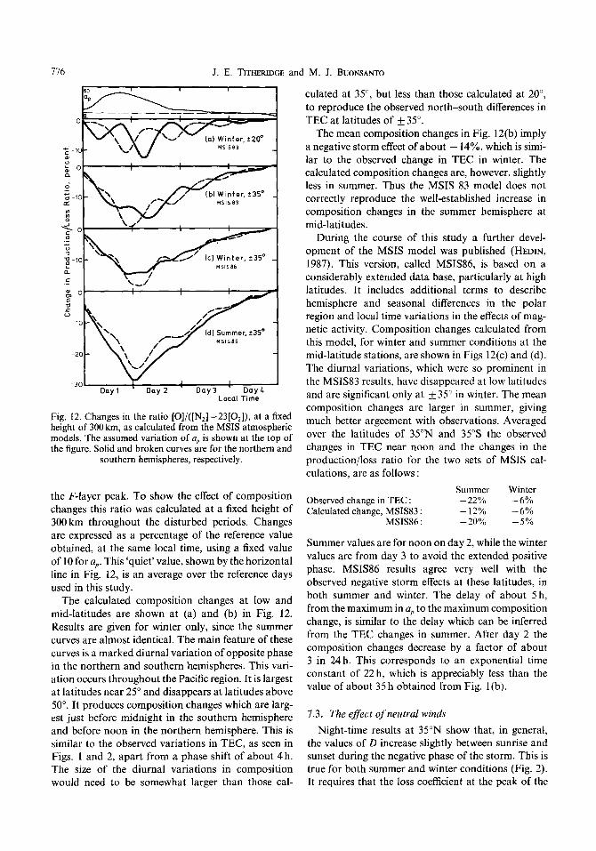
J. E. TITHERIDGE and M. J. BUONSANTO
,_c-‘/’ Icl Winter, +35O
I I ’ Day3 ’ Day6
c
Local Time
Fig. 12. Changes in the ratio [O]/([NZ] +23[0,]), at a fixed height of 300 km, as calculated from the MSIS atmospheric models. The assumed variation of ap is shown at the top of the figure. Solid and broken curves are for the northern and
southern hemispheres, respectively.
the F-layer peak. To show the effect of composition
changes this ratio was calculated at a fixed height of 300 km throughout the disturbed periods. Changes
are expressed as a percentage of the reference value obtained, at the same local time, using a fixed value of 10 for up. This ‘quiet’ value, shown by the horizontal
line in Fig. 12, is an average over the reference days used in this study.
The calculated composition changes at low and
mid-latitudes are shown at (a) and (b) in Fig. 12. Results are given for winter only, since the summer curves are almost identical. The main feature of these curves is a marked diurnal variation of opposite phase in the northern and southern hemispheres. This vari- ation occurs throughout the Pacific region. It is largest at latitudes near 25” and disappears at latitudes above 50”. It produces composition changes which are larg- est just before midnight in the southern hemisphere and before noon in the northern hemisphere. This is similar to the observed variations in TEC, as seen in Figs. 1 and 2, apart from a phase shift of about 4h. The size of the diurnal variations in composition would need to be somewhat larger than those cal-
culated at 35”, but less than those calculated at 20”,
to reproduce the observed north-south differences in TEC at latitudes of _+ 35”.
The mean composition changes in Fig. 12(b) imply a negative storm effect of about - 14%, which is simi- lar to the observed change in TEC in winter. The calculated composition changes are, however, slightly less in summer. Thus the MSIS 83 model does not correctly reproduce the well-established increase in composition changes in the summer hemisphere at mid-latitudes.
During the course of this study a further devel- opment of the MSIS model was published (HEDIN, 1987). This version, called MSIS86, is based on a considerably extended data base, particularly at high latitudes. It includes additional terms to describe hemisphere and seasonal differences in the polar region and local time variations in the effects of mag- netic activity. Composition changes calculated from this model, for winter and summer conditions at the mid-latitude stations, are shown in Figs 12(c) and (d). The diurnal variations, which were so prominent in
the MSIS83 results, have disappeared at low latitudes and are significant only at + 35” in winter. The mean composition changes are larger in summer, giving much better argeement with observations. Averaged
over the latitudes of 35”N and 35”s the observed changes in TEC near noon and the changes in the
production/loss ratio for the two sets of MSIS cal- culations, are as follows :
Summer Winter Observed change in TEC : -22% -6% Calculated change, MSIS83 : - 12% -6%
MSIS86 : -20% -5%
Summer values are for noon on day 2, while the winter
values are from day 3 to avoid the extended positive phase. MSIS86 results agree very well with the observed negative storm effects at these latitudes, in both summer and winter. The delay of about 5 h, from the maximum in a, to the maximum composition change, is similar to the delay which can be inferred from the TEC changes in summer. After day 2 the composition changes decrease by a factor of about 3 in 24 h. This corresponds to an exponential time constant of 22 h, which is appreciably less than the value of about 35 h obtained from Fig. l(b).
1.3. The effect of neutral winds
Night-time results at 35”N show that, in general, the values of D increase slightly between sunrise and sunset during the negative phase of the storm. This is true for both summer and winter conditions (Fig. 2). It requires that the loss coefficient at the peak of the

Northern and southern hemisphere TEC storm behaviour 111
F-layer is less than the value under quiet conditions.
This could be due to large diurnal changes in com-
position, or to lifting of ionisation in the northern hemisphere at night.
The dawn to dusk electric field will cause some
vertical drift, but this is cancelled out within a few hours by ion drag effects which leave a net horizontal motion (MATUURA, 1972; RISHBETH et al., 1978; BEHNKE et al., 1985). Thus appreciable lifting by electric fields will occur only when the fields are chang- ing, and is unlikely to be important during the slow recovery phase. Lifting caused by east-west electric fields will also be similar in both hemispheres, so can- not readily account for the observed north-south differences in storm response.
Lifting of ionisation by enhanced equatorward winds will be similar in both hemispheres. Because of the large eastward declination, however, zonal winds
have opposite effects at 35”N and 35°K Westward winds during the night would produce increased loss
rates in the southern hemisphere and decreased loss rates in the northern hemisphere, as the ionisation is moved to lower or greater heights. Similarly the increased daytime values of TEC in the southern hemisphere could be produced by enhanced eastward
winds. These zonal winds should be large iu winter and reduced by a factor of about 5-10 in summer, to fully account for the observed hemispherical differ- ences in TEC storm response.
Winds blowing from the polar regions will acquire an appreciable westward component, at middle and low latitudes, because of the Earth’s eastward rotation. The model calculations of BLANC and RICH- MOND (1980) show that, at a latitude of 45”, the west- ward velocity becomes greater than the equatorward velocity about 5 h after the onset of aurora1 heating. The winds are larger at night, when ion drag is least, with westward velocities of the order of 1OOm SK’. This agrees with the airglow results of YACI and DYSON (1985b) who found predominantly westward velocities of about 100 m s- ’ for about 4 h near mid- night, at a latitude of 37”s during magnetic distur- bances. HERNANDEZ and ROBLE (1984) found similar westward winds, with velocities of 10@400ms~‘, during a storm at 40”N.
Assuming equal velocities for the equatorward and westward components, and a magnetic declination of 17” (corresponding to the mean value at Auckland and Stanford), we obtain a field aligned wind which is twice as large in the northern hemisphere. Thus we expect the lifting of ionisation by disturbance winds to be twice as large at 35”N as at 35”S, at least during the first night of the disturbance. This provides an adequate explanation for the earlier onset of negative
storm effects at 35”S, near midnight of the first day
(Figs. 1 and 2). If westward winds persist throughout
the storm recovery phase they could also account for the abnormally slow night-time decay at 35”N, and
the rapid decay at 35‘S, noted in Section 7.1.2.
7.4. North-south d$erences in magnetic activity
A hemispherical asymmetry between the geo- magnetic activity indices a, and a,, for the northern and southern hemispheres, was reported by SHAH et al. (1984). The asymmetry was near 60% at the June solstice when, they concluded, the geomagnetic field is also more prone to disturbance. They defined the
percentage asymmetry as lOO(a, - a,)/[(a, + u,)/2], so an asymmetry of 60% implies a, z 1.9 a,.
Using K, and K, data for the 53 storms observed both in Auckland and Stanford TEC, we obtained values for the sums Z K,, and C KS over the first 24 h of
each storm. These results gave mean values for the 32 ‘June’ storms of 91 f3 for K, and 88f4 for KS. For the 21 ‘December’ storms the mean values were K, = 98 + 3 and KS = 97 f 1. The differences between K, and KS are not significant, so a hemispherical asym- metry in geomagnetic activity is not responsible for the observed north-south differences in TEC storm behaviour.
8. CONCLUSIONS
Mean storm response patterns are determined from TEC observations during 58 storms at similar mid-
latitude stations in the northern and southern hemi- spheres. The main features are similar in both hemi- spheres, at latitudes of 235”. The initial positive phase, on the afternoon of day 1, increases TEC by 8-10% in summer and by more than 25% in winter. The following negative phase gives changes in TEC of about -20% in summer and -8% in winter. The
transition from the positive phase to the negative phase is very rapid in summer, occurring in the first 8 h of day 2. In winter the transition takes nearly
24 h. The following recovery phase is approximately exponential with a time constant of 35 h, and is com- plete by about day 5. The size of the negative effect, in
both seasons, is similar to that expected from known composition changes as included in the MSIS86 atmo- spheric model. The recovery time is, however, 50% longer than that of the model composition changes.
The changes with storm size are also similar in the two hemispheres. In winter there is a large positive phase under all conditions, with an increase in TEC which is roughly proportional to the increase in a,. In summer there is an appreciable positive phase only

778 J. E. TITHERIDGE and M. J. BUONSANTO
for the larger storms, with K, > 6. The mean size of the negative phase is independent of the size of the disturbance, for both seasons and both stations. Thus storms with maximum Kp values of about 5 cause large changes in composition at latitudes of f 35”, but these changes show little further increase for larger storms.
There are a number of significant differences between the two hemispheres. Overall the changes at 35”s are more positive (or less negative) than those at 35”N. In undisturbed conditions, winter day values of TEC are about 80% greater in the northern hemi- sphere ; this difference is caused primarily by known differences in atmospheric composition. The overall tendency for more positive storm response patterns at 35”s therefore suggests that increased mixing of the atmosphere, during disturbed conditions, tends to reduce the normal difference in composition between the two hemispheres.
At 35”S, many daytime results (particularly for large winter storms) correspond to a decrease in the loss coefficient 8, to less than the undisturbed value. On all winter nights the results for 35”s show an enhanced loss rate, beginning near sunset. This cor- responds to an increase in the effective loss coefficient /I (at the peak of the layer) of 20%, 10% and 5% on successive nights during the storm recovery phase. These changes are about twice as large as those expected from composition changes included in the MSIS86 atmospheric model. The two effects lead to a diurnal variation which is seen in most of the results at 35”S, and dominates all other effects during large winter storms.
At 35”N there is no increase in the effective loss coefficient at night, in winter or summer, although the daytime results imply a normal increase in fl. Thus the results show a diurnal anomaly which is of opposite phase in the two hemispheres (and is larger at 35”s). The diurnal variations persist throughout the storm recovery phase, so an explanation involving electric fields seems unlikely. The results could be caused by a large diurnal change in composition, of opposite sign in the two hemispheres, persisting throughout the storm period. Variations included in the empirical MSIS83 atmospheric model went some way to fulfil- ling this requirement, but these changes have almost disappeared in the more recent MSIS86 model. Alter- natively the results could be due to enhanced winds, westward at night and eastward during the daytime. Winds of this type have been observed in both hemi- spheres, during the first day of a magnetic storm, but their persistence throughout the storm period is unconfirmed.
The positive storm phase is larger at 35”s and
occurs several hours earlier, so that the mean increase at noon on day 1 is about twice as large in the southern hemisphere. The faster response requires a more rapid lifting of the ionisation in the southern hemisphere. With a large eastward magnetic declination, at both stations, this north/south asymmetry could be pro- duced by a large eastward component in the initial daytime wind. During the following night the winds will acquire a large westward component, as discussed in Section 7.3. This westward wind, in conjuction with the eastward declination, causes the onset of the negative phase to occur a few hours earlier in the southern hemisphere.
Storms with a sudden commencement during the sunlit hours produce an increase of about 30% in TEC at both stations. In summer this is followed by a rapid overnight decay and a large negative effect on day 2. The winter results for 35”s also decay rapidly near midnight. At 35”N, however, the positive effect is sustained throughout the night and to about noon of the next day. This difference probably results from the large westward winds which are expected at night about 5 h after a period of strong magnetic activity.
When a sudden commencement occurs at night, the ionospheric response on the following day is com- pletely different at 35”s and 35”N for corresponding seasons. The observed changes are best described as an annual effect. On the day following a night-time sudden commencement, continuing magnetic activity causes a large increase in TEC for storms near the June solstice and a decrease for storms near December. Both changes are several times larger in the southern hemisphere. The same effect is apparent at latitudes of k 20”. This annual variation may relate to changes in the electron density in the plasmasphere, which is larger by a factor of 2 in June (XIA~TING and CAUDAL, 1987).
Results from 28 storms at latitudes of f20” show an appreciable negative phase only for summer con- ditions at 20”N. Positive effects are generally larger in the southern hemisphere, lasting for about 3 days at 20’S and 1 day at 20”N. TEC is normally larger at 20”N, so storm effects again act to reduce the differ- ence between the two hemispheres. In general the fluctuations in TEC are highly correlated at the two low latitude stations. This correlation often extends to 35”N, and less commonly to 35”s. The variations from storm to storm are also much larger at low latitudes. Eleven of the 28 storms showed large posi- tive effects persisting for 4 days. These storms show the same diurnal variation, with a minimum before sunrise, that was observed at 35”s. They also tend to produce large increases in TEC at 35’S throughout the storm period. This group includes 80% of the

Northern and southern hemisphere TEC storm behaviour 119
storms in the months November-April, but only 12% of the South Pacific, Suva, Fiji. Thanks are also due to of storms in the remaining 6 months. A. V. DAROSA (Stanford University) and T. H. ROELOFS
(University of Hawaii) for making their TEC results avail- able for this study, and to A. E. HEDIN (Goddard Space
Acknowledgements-This research benefited by a grant of Flight Center) and the World Data Center for Rockets and study leave to one of us (M. BUONSANTO) from the University Satellites for providing the MSIS computer program.
REFERENCES
BASU S., GUHATHAKURTA B. K. and BASU S. 1975 Ads GCophys. 31,497. BEHNKE R., KELLEY M., GONZALES C. 1985 J. geophys. Res. 90,4448.
and LARSEN M. BLANC M. and RICHMOND A. D. 1980 J. geophys. Res. 85, 1669. BLUM P. W. and HARRIS I. 1975 J. atmos. terr. Phys. 31,213. BUONSANTO M. J., MENDILLO M. and 1979 Ads Geophys. 35, 15.
KLOBUCHAR J. A. CHANDRA A. and SINHA A. K. CHANDRA S. and SPENCER N. W. DAVIES K. and RUSTER R. DICKINSON R. E., RIDLEY E. C. and ROBLE R. G. DUNCAN R. A. ESSEX E. A., MENDILLO M., SCHODEL J. P.,
KLOBUCHAR J. A., DAROSA A. V., YEH K. C., FRITZ R. B., HIBBERD F. H., KERSLEY L., KOSTEZR J. R., MAT~OUKAS D. A., NAKATA Y. and ROELOFS T. H.
EVANS J. V. GOODMAN J. M. HARGREAVES J. K. and BAGENAL F. HEDIN A. E., SPENCER N. W., MAYR H. G. and
1974 J. geophys. Res. 19, 1916. 1976 J. geophys. Res. 81, 5018. 1976 Planet. Space Sci. 24, 867. 1981 J. geophys. Res. 86, 1499. 1969 J. atmos. terr. Phys. 31, 59. 1981 J. afmos. terr. Phys. 43, 293.
1970 J. atmos. terr. Phys. 32, 1629. 1968 Planet. Space Sci. 16,95 1. 1977 J. geophys. Res. 82,73 1. 1981 J. geophys. Res. 86,3515.
PORTER H. S. HEDIN A. E. HEDIN A. E. HEDIN A. E., BAUER P., MAYR H. G.,
1983 J. geophys. Res. 88, 10 170. 1987 J. geophys. Res. 92,4649. 1977 J. geophys. Res. 82, 3 183.
CARIGNAN G. R., BRACE L. H., BRINTON H. C., PARKS A. D. and PELZ D. T.
HERNANDEZ G. and ROBLE R. G. 1976 J. geophys. Res. 81, 5173. HERNANDEZ G. and ROBLE R. G. 1984 J. geophys. Res. 81,9049. HIBBERD F. H. and Ross W. J. 1967 J. geophys. Res. 72,533l. HUANG Y.-N., NAJITA K., ROELOFS T. H. and 1974 J. atmos. terr. Phys. 36, 9.
YUEN P. C. JONES K. L. JONES K. L. JONES K. L. and RISHBETH H. JUNG M. J. and PR~LSS G. W. KANE R. P. KANE R. P. KILLEEN T. L. and ROBLE R. G. KING G. A. M. KLOBUCHAR J. A., MENDILLO M., SMITH F. L. III,
FRITZ R. B., DAROSA A. V., DAVIS M. J., YUEN P. C.. ROELOFS T. H., YEH K. C. and FLAHERTY B. J.
1971 J. atmos. terr. Phys. 33, 379. 1973 J. atmos. terr. Phys. 35, 1515. 1971 J. atmos. terr. Phys. 33, 391, 1978 J. atmos. terr. Phys. 40, 1347. 1973 J. atmos. terr. Phys. 35, 1953. 1975 J. atmos. terr. Phys. 37, 601. 1986 J. geophys. Res. 91, 11291. 1971 J. atmos. terr. Phys. 33, 1223. 1971 J. geophys. Res. 16,6202.
KOHL H., KING J. W. and ECCLES D. Kotadia K. M. KOTADIA K. M. and JANI K. G. LANZEROTTI L. J., COGGER L. L. and MENDILLO M MATSUSHITA S. MATUURA N. MAYR H. G. and HEDIN A. E. MAYR H. G. and VOLLAND H. MAYR H. G. and VOLLAND H. MAZAUDIER C. and Bernard R. MENDILLO M.
1969 J. atmos. terr. Phys. 31, 1011. 1965 J. atmos. terr. Phys. 21, 723. 1967 J. atmos. terr. Phys. 29, 661. 1975 J. geophys. Res. 80, 1287. 1959 J. geophys. Res. 64, 305. 1972 Space Sci. Rev. 13, 124. 1977 J. geophys. Res. 82, 1227. 1973 J. geophys. Res. 78,225 I. 1974 J. atmos. terr. Phys. 36, 2025. 1985 J. geophys. Res. 90,2885. 1971 Nature Phys. Sci. 234,23.
780 J. E. TITHERIDGE and M J. BUONSANTO
MENDILLO M. and KLOBUCHAR J. A. MENDILLO M., KL~BUCHAR J. A. and
HAJEB-HOSSEINIEH H. MENDILLO M., PAPACIANNIS M. D. and
KLOBUCHAR J. A.
1975 J. geophys. Rex 80,643. 1974 Planet. Space Sci. 22, 223.
1970 Radio Sci. 5, 895.
MILLER N. J., MAYR H. G., SPENCER N. W. 1984 J. geophys. Res. 89,2389. and BRACE L. H.
NELSON G. J. and COGGER L. L. NISBET J. S., WYDRA B. J., REBER C. A.
1971 Planet. Space Sci. 19, 761. 1977 Planet. Space Sci, 25, 59.
and LUTON J. M. PAPAGIANNIS M. D., MENDILLO M. 1971 Planet. Space Sci. 19, 503.
and KLOBUCHAR J. A. POTTER W. E., KAYSER D. C. and NIER A. 0. PR~LSS G. W. PRiiLSS G. W. PRoLSS G. W. PR~LSS G. W. and VON ZAHN U. PR~LSS G. W. and VON ZAHN U. PR~LSS G. W., VON ZAHN U. and RAITT W. J. RAJARAM G. and RASTOGI R. G. RISHBETH H., GORDON R., &ES D. and
1979 J. geophys. Res. 84, 10. I977 J. geophys. Res. 82, 1635. 1980 Rev. Geophys. Space Phys. 18, 183 1987 Planet. Space Sci. 35, 807. I974 J. geophys. Res. ‘79, 2535. 1977 J. geophys. Res. 82, 5629. 1975 J. geophys. Res. 80, 3715. 1970 J. atmos. terr. Phys. 32, 113. 1985 Planet. Space Sci. 33, 1283.
FULLER-R• ~ELL T. J. RISHBETH H., GANCULY S. and WALKER J. C. G. SCHODEL J. P., DAROSA A. V., MENDILLO M.,
KLOBUCHAR J. A., ROELOFS T. H., FRITZ R. B., ESSEX E. A., FLAHERT~ B. J., YEH K. C., HIBBERD F. H., KERSLEY L., KOSTER J. R., LISZKA L. and NAKATA Y.
SEATON M. J.
1978 J. atmos. terr. Phys. 40, 767. I974 J. atmos. terr. Phys. 36, 1121.
SHAH G. N., KAUL R. K., KAUL C. L., RAZDAN H., 1956 J. atmos. terr. Phys. 8, 122. 1984 J. geophys. Res. 89, 295.
MERRYFIELD W. J. and WILCOX J. M. SIPLER D. P. and BIONDI M. A. SONG XIA~TING and CAUDAL G. SPURLING P. H. and JONES K. L. SPURLING P. H. and JONES K. L. STUBBE P. and CHANDRA S. TANAKA T. TAYLOR G. N. and EARNSHAW R. D. S. TIAN-XI H. TITHERIDGE J. E. TITHERIDGE J. E. TITHERIDGE J. E. and ANDREWS M. K. TITHERIDGE J. E. and BUONSANTO M. J. TRINKS H., FRICKE K. H., LAUX U., PR~LSS G. W. and
1979 J. geophys. Res. 84, 37. 1987 J. atmos. terr. Phys. 49, 1351. 1973 J. atmos. terr. Phys. 35,921. 1976 J. atmos. terr. Phys. 38, 1237. 1970 J. atmos. terr. Phys. 32, 1909. 1979 J. atmos. terr. Phys. 41, 103. 1969 J. atmos. terr. Phys. 31,2 11. 1985 J. atmos. terr. Phys. 47, 1031. 1973 Planet. Space Sci. 21, 1775. 1974 J. atmos. terr. Phys. 36, 1249. 1967 Planet. Space Sci. 15, 1157. 1983 J. atmos. terr. Phys. 45, 683. 1975 .I. qeophys. Res. 80, 4571.
VON ZAHN U. VOLLAND H. YAGI T. and DYSON P. L. YACI T. and DYSON P. L.
1979 J. atmos. terr. Phys. 41, 853. 1985a J. atmos. terr. Phys. 47, 1075. 1985b’ Planet. Space Sci. 33,46 1.
Reference is also made to the following unpublished material:
MENDILLO M. 1973
MENDILLO M. 1975
MENDILLO M. 1976
MENDILLO M. 1978
Magnetospheric Convection at Ionospheric Heights, AFCRL Tech. Rep. -73-0358, AFCRL, Hanscom AFB, MA, 1973.
Beacon Satellite Investigations of the Ionosphere Struc- ture and ATS-6 Data, Vol. II, Izmiran, Moscow, p. 60.
Proceedings of COSPAR Symposium on the Geo- physical Use of Satellite Beacon Observations (MEN- DILLO M., ed.), Boston Univ., Boston, MA, 1976, p. 307.
Behavior of the Ionospheric F-Region During Geo- magnetic Storms, AFGL Tech. Rept. -78-0092(11), AFGL, Hanscom AFB, MA, 1978.