A Comparison of Fixed and Variable Block

Allocation in two Java Virtual Machines

by Markus Goffart, Gerhard W. Dueck, and Rainer Herpers

TR 12-218, July 20, 2012

Faculty of Computer Science University of New Brunswick

Fredericton, NB, E3B 5A3 Canada

Phone: (506) 453-4566 Fax: (506) 453-3566 Email: fcs@unb.ca

http://www.cs.unb.ca

1

Abstract

This paper compares the memory allocation of two Java virtual machines,namely Oracle Java HotSpot VM 32-bit (OJVM) and Jamaica JamaicaVM(JJVM). The basic difference of the architectures is that the JJVM uses fixedsize block allocation on the heap. This means that objects have to be split intoseveral connected blocks if they are bigger than the specified block-size. On theother hand, for small objects a full block must be allocated. The paper containsboth theoretical analysis and experimental results on the memory-overhead.The theoretical analysis is based on specifications of the two virtual machines.The experimental analysis is done with a modified JVMTI Agent together withthe SPECjvm2008 Benchmark. The results are summarized in a diagram. Fromthis diagram, it can be seen which block size should be used for a given datasize.

Contents

1 Introduction 2

2 Methodology 42.1 Architecture of Objects in OJVM and JJVM . . . . . . . . . . . 42.2 JVMTI-Tool . . . . . . . . . . . . . . . . . . . . . . . . . . . . . 72.3 Benchmarks . . . . . . . . . . . . . . . . . . . . . . . . . . . . . . 7

3 Results of SPECjvm2008-Benchmarks 9

4 Optimal Parameter Setting 114.1 Comparison of Overhead Between all Block-Sizes . . . . . . . . . 114.2 Block-Size n for Specific Standard Objects . . . . . . . . . . . . . 124.3 Block-Size n for Specific Array Objects . . . . . . . . . . . . . . . 144.4 Which Block-Size for a Specific Program? . . . . . . . . . . . . . 14

5 Conclusion 16

6 Future Work 18

1

Chapter 1

Introduction

A very important part of Java virtual machines is the garbage collector. It isresponsible for the reorganization of the objects on the heap during the runtimeof the JVM.

Two of the most recent developed and standard garbage collectors (GC) (i.e.Java virtual machines) that were developed for real-time applications, are theJJVM of the company aicas [1] and the Concurrent Mark and Sweep Collector(CMS) in the OJVM [13]. The JJVM tries to get short and bounded pause timesin the first step in the GC-process in hard real-time systems [8]. This means thatthere are predictable execution times of stop-the-world phases. Whereas theOJVM avoids long stop-the-world phases with a concurrent garbage collector.This means that most of the garbage collection is done concurrently with theexecution of the program. Most GCs need four steps to clean and compactthe heap. These are the Root Scanning, Mark, Sweep, and Compaction. Thebasic difference between the garbage collectors of OJVM and JJVM is that theJJVM does not have a compaction phase. It becomes redundant due to the useof fixed-size blocks for the allocation of new objects on the heap [5][6]. However,the allocation of objects becomes more complex because the GC needs to trackthe free space and also has to split bigger objects into several fixed-size partsif an object is larger than the fixed-size block. Siebert measured the allocationtime and could show that the time-overhead is low (< 1 µs) [7].

Thus, the runtime of the JJVM seems to be quite good but what are thedisadvantages is this case? The new architecture of the JJVM causes some addedcosts. First, there is wasted space due to the fact that the object may not fillan exact multiple of the fixed-size blocks. Second, links must be kept for splitobjects. These structures also affect the runtime because the GC may need toscan several blocks for one object and keep track of the additional informationin chunks. Although Siebert conducted a first analysis on the JJVM, moreresearch on this topic is necessary. He mentioned that the benchmarks used donot reflect real-time applications and this should be changed in future work.

This paper provides a detailed analysis of the JJVM memory allocationscheme. For this purpose, a profiler tool was implemented with the Java Virtual

2

Machine Tool Interface (JVMTI) [3] to analyze and compare the heap of theboth virtual machines. This paper also describes how it is possible to find thebest block-size n in the JJVM for any object.

The paper starts with some background information necessary to understandthe basic differences between the object-sizes in JJVM and OJVM. Then, ashort description of the modified JVMTI-profiler “hprof” that was used for theanalysis follows. The two benchmarks that were used in this work are presented.After this, the results of the theoretical and experimental analysis are presented.The paper ends with some concluding remarks.

3

Chapter 2

Methodology

2.1 Architecture of Objects in OJVM and JJVM

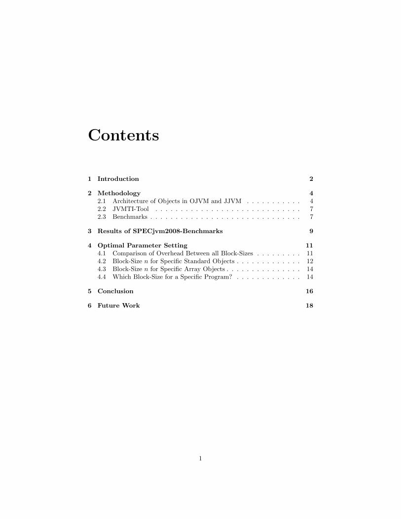
Figures 2.1 and 2.2 show the architecture of objects in the OJVM and JJVMrespectively. There is a difference between standard objects and array objectsin both machines. In the OJVM, the standard object has a two words-headerfollowed by the actual data, whereas the array-objects has a three words-headerfollowed by the data. While the first two fields in both structures containinformation such as hash-code, color-flag and a reference to the class of theobject, the third field of an array object contains the number of elements of thearray itself [4]. Together with the condition that the total size of the objectmust be a multiple of 8 bytes the total size for java objects in the OJVM is asfollows:

ssoOJVM =⌈2·smp+sdata

8

⌉· 8 [B] (standard object)

saoOJVM =⌈3·smp+nel·sdata

8

⌉· 8 [B] (array object)

(2.1)

where smp represents the size of machine-pointer (also known as word), sdatathe size of the actual data, and nel denotes the number of elements in the array.The result is given in bytes [B].

Figure 2.1: Architecture of a standard object and array object in the OJVM.

4

The storage of objects is different in JJVM and OJVM. In JJVM objects aresplit into fixed-size blocks with a length of n words (Part A of Figure 2.2 showsan empty example block). The size of the word is the same as for the OJVM –the size of a machine pointer. If an object is larger than the block-size, the dataof the object has to be split into several blocks. Also, the JJVM stores standardobjects differently than array objects. Both structures do have a so called head-block that contains additional information of the object itself and in case of anarray of the sub-structure. The head-block for standard-objects requires threewords for information such as color-flag of the object (used during the garbagecollection for marking visited objects), type of the object, and monitor of theobject (used for the monitoring-process that is available in the JJVM). Then,the data follows and it can be split over successive blocks that are connectedby a pointer to the next block (see Part B of Figure 2.2). The head-block ofthe array-object contains one more reserved word that has information aboutthe length and depth of the array-structure-tree. The data is separated in fieldsthat are located in blocks at the last level of the tree. Each block is connectedwith link-fields up to the head block (see Part C of Figure 2.2). Only the sizeof the actual data sdata of an object in the OJVM is the same as in an object inJJVM. For standard object the total number of fields (including the head-blockinformation and link-fields) that are used, is as follows:

numOfFieldsTotal =

⌈3 · smp + sdata

smp

⌉(2.2)

The following equation calculates the number of total blocks (TB) that arenecessary to provide enough space for the number of fields of Equation (2.2):

TBso =

⌈numOfFieldsTotal − 1

(n− 1)

⌉(2.3)

where n is the number of fields that has been chosen for the block-size.Then, the total size of a standard object on the heap of the JJVM (ssoJJVM )

is as follows:ssoJJVM = (TBso · n · smp) [B] (2.4)

The memory allocation of array object in the JJVM is a little bit morecomplex. To explain how the equations for the memory-allocation of an array-object in the JJVM were derived, would go beyond the scope of this paper (fordetails see [2]). First the depth of the tree is calculated regarding number offields that are used for the data sdata. The number of fields that is necessaryfor sdata is calculated first:

numOfFieldsData =

⌈sdatasmp

⌉(2.5)

Since the number of necessary fields is known, the depth of the array-structurecan be calculated with the equation as follows:

depth =

⌈log2(numOfFieldsData)− log2(n− 4)

log2(n)

⌉(2.6)

5

with n = number of fields in one block and numOfFieldsData from Equa-tion (2.5).

Now, the number of fields for an array (2.5) and the depth of the array-structure (2.6) are known. With this information it is possible to calculate thetotal number of total blocks (TB) that are used for head-block, linking blocks,and the data blocks for an array-structure as follows:

TBao = getNumBlocks(depth, numOfFieldsData) (2.7)

where getNumBlocks(d, b) = gNB(d, b) is a recursive function as follows:

gNB(d, b) =

{1 (if d = 0)gNB

(d− 1,

⌈bn

⌉)+⌈bn

⌉(if d > 0)

(2.8)

Thus, the total size saoJJVM for one array-object on the heap in the JJVMis then as follows:

saoJJVM = (TBao · n · smp) [B] (2.9)

This looks the same as for the standard object, but the derivation for the num-ber of TotalBlocks is different (TBso 6= TBao). For each block on the heap,the JJVM stores additional information in so called groups. This informationrequires some space that belongs the the size of the object. Thus, if the num-ber of TotalBlocks is known, the additional space used by the groups can becalculated. The additional space is reserved for the reference-flag for each wordin the block (n · 1 bit), the color-flag (4 bit) and the grey-link that shows for 8blocks the reference to the next group that has at least one grey-marked object.The grey link is as big as one machine pointer and is divided by the number ofthe blocks in one group (which is 8). So, the total amount of memory for anobject is:

TotalMemory = TB ·(

(n · smp) +smp + n+ 4

8

)[B] (2.10)

with

TB =

{TBso (for standard object)TBao (for array object)

(2.11)

Compared to the object-size in the OJVM, it should be mentioned that thereis some memory-overhead in the JJVM that is produced by linking fields, re-maining empty fields (because of the fixed-size blocks), and additional groupinformation. The memory-overhead is the TotalMemory minus the three (forstandard objects) or four fields (array objects) of header information, and minusthe data-size of the object itself. This leads to the following memory-overhead-equations for standard objects (ohso) and array objects (ohao):

ohso = (TBso · n− 3− nOFD) · smp [B] + ohgen · TBso [B]ohao = (TBao · n− 4− nOFD) · smp [B] + ohgen · TBao [B]

(2.12)

where ohgen is the general size of memory that is used for each block for thegroup information as follows:

ohgen =

(smp + n+ 4

8

)[B]

6

2.2 JVMTI-Tool

The Java Virtual Machine Tool Interface (JVMTI) provides a library to createso called agents to analyze the states of any program during the runtime ofthe virtual machine. In this paper, the agent “hprof” given by the demos ofthe JVMTI was modified. This agent only needs minor changes to cover thenecessaries for the analysis of the memory between the OJVM and the JJVM. Inthis case is used the possibility to get information such as size and type of eachobject that has been allocated by the profiled application. This information issaved and later used for the recalculation of standard and array object-sizes tothe memory needs of the JJVM because the profiling takes place only duringthe runtime with the OJVM. Since it was not possible to get a runnable JJVM,the recalculation step was necessary to get a comparable base. This means thatthe size of standard objects and array objects in the OJVM is recorded and thenrecalculated to the memory-needs in the JJVM with the help of the theoreticalcalculations in Section 2.1. With the help of the type of the object and theknown header information (2 fields for standard objects and 3 fields for arrayobjects) it is possible to separate the actual data-size sdata and use it for thecalculations of memory used and overhead in the JJVM.

2.3 Benchmarks

The objective of this paper is to check how the memory allocation for dif-ferent block-sizes n looks like for real life applications and for specific caseswhere it is possible to specify the general size of the allocated objects, becauseSiebert did not test with real life benchmarks (as mentioned in the introduc-tion). Two real life applications were found in the SciMark and Sunflow of theSPECjvm2008 Benchmark [11, 12]. This is also the reason why only two of thewhole SPECjvm2008-Benchmark-set were used for this paper. The SciMark isa performance test on the CPU and the Sunflow is a multi-threaded renderer totest graphic visualization.

The memory usage for the two benchmarks (in both virtual machines) andthe memory-overhead for four different block-sizes (n = 8, n = 16, n = 32, andn = 64) in the JJVM are calculated.

7

Figure 2.2: Architecture of a fixed-size block A), standard object B) and arrayC) object in the JJVM.

8

Chapter 3

Results ofSPECjvm2008-Benchmarks

Figure 3.1 shows the results for the Sunflow- and the SciMark-benchmark. Eachfigure shows a diagram with the size of the used memory for the OJVM and foreach defined block-size (n = 8, n = 16, n = 32, and n = 64 fields) in the JJVM.The diagram also shows how much of the used memory is overhead that wascreated by the JJVM (grey bar charts).

There is a small difference of the used data-size together with header-information(black part of the bar charts) between the OJVM and the JJVM because bothtypes of objects in the JJVM (standard object or array object) use one moreword than in the OJVM. In summary, the difference between both machinesbecomes significant. It can also be seen that the memory-overhead increaseswith the size of the blocks. A closer look into the distribution of the size ofthe objects shows that there are much more small object allocations than bigobjects allocations (around 50% of objects are lower than 25 bytes; the restis located in higher ranges up to 20 kilobyte). The logical result is that thereis less memory-overhead for smaller block-sizes than for larger block-sizes. Itshould be noted that the memory-overhead for the block-sizes n = 8 and n = 16is mostly the same in the SciMark-benchmark. The reason for this is explainedin the next Section 4.

9

Figure 3.1: Used memory and memory-overhead of Sunflow and SciMark bench-mark for different block-sizes (n = 8, n = 16, n = 32, and n = 64 fields) andfor both virtual machines. For both cases, the best block-size is n = 8 but incase of the SciMark benchmark it is also possible to use the block-size of n = 16because there are only minor differences in the memory-overhead.

10

Chapter 4

Optimal Parameter Setting

In previous chapter, some results of the memory-overhead investigation accord-ing to specific programs that the agent analyzed during the runtime were pre-sented. Now, the objective is to find the best block-size for any given programso that the memory-overhead stays as small as possible. Thus, this chapter ex-plains how to get the best block-size for a given program. Section 4.1 presentssome further analysis on the memory-overhead for the first four successive block-sizes with n = 8, n = 16, n = 32, and n = 64. It shows that there are someranges that have the same memory-overhead for two or more block-sizes at spe-cific data-sizes. This means that it does not matter which block-size is chosenbecause the memory-overhead would be the same for some data-sizes. This factmakes the exact calculation for the correct block-size a little more challenging.Sections 4.2 and 4.3 show how to get the block-size for a specific data-size foreach type of data structures in the JJVM. Finally, the overview for the firstfour block-sizes is presented and the experimental results are compared to thisdiagram.

4.1 Comparison of Overhead Between all Block-Sizes

The Figures 4.1 and 4.2 show the memory-overhead for both types of datastructures in the JJVM. It can be seen in both cases that in most cases thememory-overhead varies according to the different block-sizes for one specificdata-size but there are also some ranges, where the memory-overhead does notchange for all four tested block-sizes. For example in the range between 416 and440 bytes the memory-overhead for all block-sizes of the standard objects hasmostly the same size for the first four block-sizes (n = 8, n = 16, n = 32, andn = 64 fields). A synthetic test-program that creates objects with the data-sizeof 424 bytes (this data-size lays in the previous mentioned range) showed thatthe overhead indeed became the same size for all four block-sizes.

There are also some data-sizes where the memory-overhead gets smaller for

11

Figure 4.1: Comparison of overhead in standard objects between different block-sizes (n = 8, n = 16, n = 32, and n = 64 fields) and the same data-size. It showsthat it makes no sense to use smaller block-sizes for bigger data-sizes in generalbecause the memory-overhead becomes bigger than for bigger block-sizes (e.g.,an object with the data-size around 3000 bytes creates an memory-overhead ofaround 650 bytes for the block-size of n = 8 and only around 400 bytes forn = 64).

one block-size than for another one, but for the next few data-sizes the size of thememory-overhead for the same block-sizes switches their order. For example,for the data-size of 496 bytes, the memory-overhead for the blocksize n = 32is around 158 bytes and for the block-size n = 64 around 2 bytes, but for thedata-size of 500 bytes, the memory-overhead for the block-size n = 32 is almostconstant and the memory-overhead of n = 64 increases up to around 283 bytes.Thus, in the first case the block-size n = 64 would have been chosen, whereasin the second case the block-size of n = 32 would have been chosen because ofthe lower memory-overhead in both cases.

Because of the previously mentioned overlapping area and the switching ofthe memory-overhead-sizes, it is not possible to predict exactly for which data-size-range the best block-size should be taken. For one specific data size thebest block-size can be chosen but not for a whole range that is actually moreapplicable for general programs because objects of different sizes are usuallyallocated and not only from one specific size. Some more specific analysis onthe memory-overhead and the results for such ranges is explained in the nextSections 4.2 and 4.3.

4.2 Block-Size n for Specific Standard Objects

To get the recommended blocksize n for any data-size sdata, there are severalsteps necessary. First, to evaluate how big the differences between the neigh-bouring block-sizes in the memory-overhead would be, the difference betweenthe memory-overhead of the current block-size n and the memory-overhead of

12

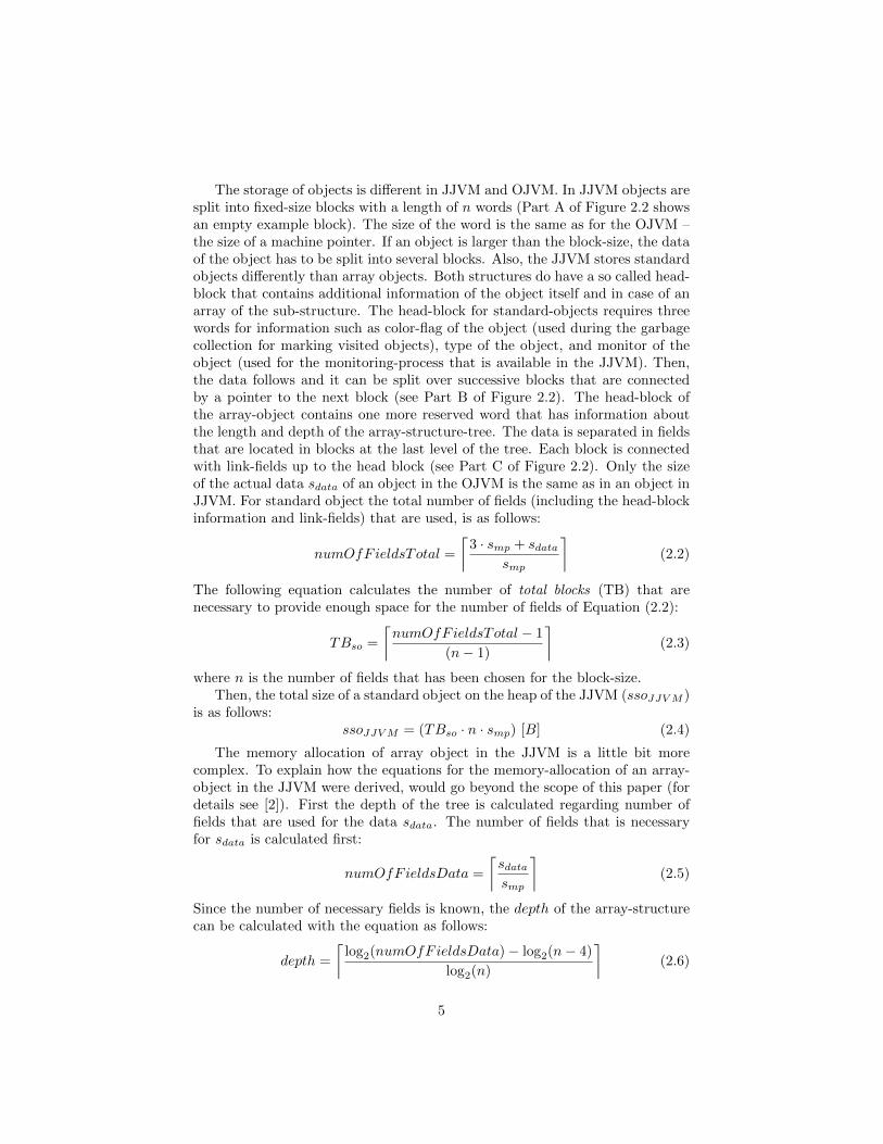
Figure 4.2: Comparison of overhead in array objects between different block-sizes (8, 16, 32, and 64) and the same data-size. It shows that it makes no senseto use smaller block-sizes for bigger data-sizes in general because the memory-overhead becomes bigger than for bigger block-sizes (e.g., an object with thedata-size around 3000 bytes creates an memory-overhead of around 700 bytesfor the block-size of n = 8 and only around 300 bytes for n = 32

the next successive block-size (n · 2) is calculated. If the difference gets belowzero, the memory-overhead of the successive block-size is bigger than the cur-rent one. With this information it can be seen at which data-size it is better toswitch from the smaller block-size n to the next block-size n · 2 to avoid highmemory-overhead. There are always two thresholds that define three operatingregions for block-size allocations:

• All data-sizes up to the first threshold:For all data-sizes up to the first threshold, should definitely be taken thesmaller block-size because then the memory-overhead is also smaller forthe smaller block-size.

• All data-sizes bigger than the second threshold:For this, the memory-overhead never becomes smaller than zero, whichmeans that the bigger block-size (n ·2) has a lower memory-overhead thanthe smaller block-size n and should be taken.

• All data-sizes between the two thresholds:The difference of the memory-overhead of the data-sizes between those twothresholds varies from negative to positive values and vice versa. Thismeans, for this range, a general decision cannot be made if the smalleror bigger block-size should be taken. Usually, implementations do notallocate objects with exactly the same size, but might be located in aspecific range. For this, a more simplified representation of the data isused. One simplified representation is found by the linear regression linethat shows the memory-overhead-difference between two block-sizes aslinear slope. The regression line intersects with the x-axis at one point.

13

This point is chosen as threshold for switching the block-size if the data-size becomes bigger in this paper.

For example, in the analysis to this paper the linear regression of the memory-overhead-difference between the block-sizes n = 8 and n = 16 for standardobjects shows an intersection with the x-axis at 16 bytes (0 = 0.098·x−15.914⇔x = 15.914

0.098 = 163, 4). This is then the recommended maximum of the data-sizefor the block-size n = 8.

4.3 Block-Size n for Specific Array Objects

The same steps as given for the calculation to get the threshold for standardobject apply for the threshold of array objects.

4.4 Which Block-Size for a Specific Program?

Figure 4.3: Recommended maximum block-size n for a specific data-size sdata.For the known distribution of the data-size it can be looked up which block-sizeis recommended regarding the ratio of standard- and array-objects.

Figure 4.3 shows the recommended block-size for a specific data-size forstandard and array objects for the first four block-sizes (n = 8 up to n = 64).The numbers are the intersection points with the x-axis of the regression-linesthat are explained in previous two sections. For any object-size, the suggestedblock-size can be read by following the slope to the next block-size of 2n (withn ∈ N>2). For example, if there is an array object allocation of the size around500 bytes, it is recommended to use the block-size of n = 32. In general,it can be said that for array objects the recommended size of the block-sizeincreased faster than for standard objects. This is because of the differentarchitecture of both types of objects. Standard objects produce less memory-overhead than array objects with the same data-size. To get the correct block-size for a program, it is necessary to analyze first the object allocations of

14

the program. One option is to analyze the distribution of the object sizes forstandard and array objects (i.e., histogram). If the size of the typical allocationof a standard and an array object is known, it can be looked up in the diagramwhich block-size matches the best.

If the problem arises that the analysis for each object type would lead to twodifferent block-size recommendations, it should be weighted which block-size isbetter regarding the memory-overhead for the other object type. For example, ifthe data-size of standard objects would be 200 bytes but for array objects around8000 bytes then the recommended block-size would be n = 8 for standard objectsand n = 64 for array objects. If the block-size of 64 is chosen, the memory-overhead of standard objects is in general too high because there is always a highnumber of unused fields in smaller object-allocations. Otherwise, if the block-size of n = 8 is chosen, the memory-overhead for the array-list increases a lotbecause of additional depths and linking fields that cause a memory-overhead.If the tendency of the object allocations is known (e.g., 25% array objects and75% standard objects or vice versa), it is possible to find the block-size by justusing the assisting lines (e.g., 75% for the previous mentioned case). The higherthe percentage of the distribution between array-object and standard-objectis, the higher is the number of standard object allocations. 50% means thatthe number of allocations for standard and array objects is the same. If thetendency is not known, it is recommended to use the 50% line which is a goodassumption, because this works well for all mentioned examples in this paper.

If larger block-sizes are chosen, the total runtime of the garbage collectioncycle decreases because there are less blocks that has to be marked. This isactually an advantage for the purpose of the JJVM to have small and predictablerun-times in the GC. On the other hand, objects that are smaller than the sizeof the block, create more memory-overhead. So, again, this remains at handsof the programmer to choose a block-size and he has to decide if he wants lessmemory needs or less total GC times.

In general, it can be said that the block-size of n = 8 is a good size becausein most applications, the size of the objects do not increase beyond 37 bytesfor standard objects or 163 bytes for array objects. These are maximum sizesfor the data that fits for the block-size n = 8 for standard and array objects,respectively (compare Figure 4.3). This can also be seen in the two tested reallife applications SciMark and Sunflow. All test results show that the block-sizeof n = 8 is the best because of the smallest memory-overhead. Only in specialcases, it is necessary to choose another block-size or it does not matter (e.g.,the synthetic test program that allocates objects with the size of 424 bytes).

15

Chapter 5

Conclusion

The results presented in this paper lead to the conclusion that the block-size ofn = 8 works the best for the most programs because they usually have manyobjects that are below the size of 163 bytes. This is the upper bound for standardobjects and the block-size n = 8 in the JJVM (see Figure 4.3). The upper boundfor the recommended block-size of standard objects is always higher than for thearray objects. This is because of the higher memory-overhead that array-objectsproduce than for standard-objects for the same data-size.

If the tendency of the distribution between standard and array objects isknown, the programmer can use the assisting lines in Figure 4.3. Unfortunately,objects are seldom uniform, but it turns out that all programs in this paper andthe results of them show that they are good matches for the 50%-line. Moreexperiments are required to confirm that the distribution of standard and arrayobjects is equal for the general case.

Although the JJVM provides a garbage collection for real-time systems withcritical time constrains, the costs for the necessary memory of the garbage col-lection are higher than in the OJVM. There was a minimum average of 20%increase in memory-use in the JJVM when it is compared with OJVM for allprograms and benchmarks used in this paper and when the block-size was chosenthat produces the smallest memory-overhead. This is definitely a disadvantageof the JJVM.

For programs that have more larger size objects, larger block sizes are rec-ommended, since the memory-overhead for accessing large blocks is small. Thismight also be a problem because if there are two main distributions of objects(e.g., one small and one big object-distribution) that actually causes two differ-ent block-size recommendations, the programmer has to decide which block-sizehe should use in his implementation.

Regarding the two tested JVMs the conclusion is as follows: If an imple-mentation does not need a virtual machine that fits the hard real-time goals,it is recommended to use the standard OJVM. The JJVM should be taken inthe other case. The JJVM should also be taken if short and predictable GCpauses are necessary, although more memory is used. Then, the programmer

16

just needs to provide a bigger memory for the heap.

17

Chapter 6

Future Work

Siebert [8] already gave an overview of the runtime-overhead of the GC inthe JJVM but also mentioned that the benchmarks that were used do not re-flect the characteristic of real applications. The benchmarks that were used bySiebert show that the GC of the OJVM runs in average 20% faster than theJJVM [8]. Some future work should be the testing with real applications (orbenchmarks that reflects those ones) on the JJVM and compare the run-timewith the OJVM.

There should also be a more specific performance analysis regarding thechange of the the block-size. For example, it can happen that the programmerchooses a small block-size that leads in case of big objects to many small blocks-divisions that has to be checked during the GC. The bigger the objects are themore connections hast to be checked. This leads to a more time-consuming factthan it would be if the block-size would not have been chosen too small.

18

Bibliography

[1] aicas, JamaicaVM - Java Technology for Realtime, URL:http://www.aicas.com/jamaica.html, Retrieved: 8 July 2011

[2] Markus Goffart Comparison of Memory Allocation in the Jamaicaand Oracle Java Virtual Machine, Master’s Thesis, University of NewBrunswick, Fredericton, January 2012

[3] Oracle, Java Virtual Machine Tool Interface - Version 1.2, URL:http://download.oracle.com/javase/6/docs/platform/jvmti/jvmti.html, Re-trieved: 8 July 2011

[4] Oracle, Whitepaper - The Java HotSpot Performance Engine Ar-chitecture, URL: http://java.sun.com/products/hotspot/whitepaper.html,Retrieved: 25 September 2011

[5] Siebert F., The Impact of Realtime Garbage Collection on Re-altime Java Programming, Journal: Object-Oriented Real-Time Dis-tributed Computing, 2004. Proceedings, Date: 14 May 2004, Page(s): 33- 40, ISBN: 0-7695-2124-X, INSPEC Accession Number: 8302198

[6] Siebert F., Slides to: The Impact of Realtime Garbage Col-lection on Realtime Java Programming, URL: http://www.cs.uni-salzburg.at/announcements/Slides Siebert.pdf, Retrieved: 8 July 2011

[7] Siebert F., Concurrent, Parallel, Real-Time Garbage-Collection,Journal: ISMM ’10 Proceedings of the 2010 International Symposium onMemory Management, Year: 2010, ACM New York, ISBN: 978-1-4503-0054-4

[8] Siebert F., Realtime Garbage Collection in the JamaicaVM 3.0,JTRES’07 - The 5th International Workshop on Java Technologies for Real-time and Embedded Systems - JTRES 2007, 26-28 September 2007, Vienna,Austria

[9] Standard Performance Evaluation Corporation, Java Virtual MachineBenchmark, URL: http://www.spec.org/jvm2008/, Retrieved: 8 July 2011

19

[10] Standard Performance Evaluation Corporation,SPECjvm2008 User Guide; Version 1.0; Last modified: 16 April 2008,URL: http://www.spec.org/jvm2008/docs/UserGuide.html, Retrieved: 2November 2011

[11] Standard Performance Evaluation Corporation, Sunflow - Descrip-tion, URL: http://www.spec.org/jvm2008/docs/benchmarks/sunflow.html,Retrieved: 2 November 2011

[12] Standard Performance Evaluation Corporation, SciMark - Descrip-tion, URL: http://www.spec.org/jvm2008/docs/benchmarks/scimark.html,Retrieved: 2 November 2011

[13] Sun Microsystems, Memory Management in theJava HotSpot(TM) Virtual Machine, Date: April2006, URL: http://java.sun.com/j2se/reference/whitepapers/memorymanagement whitepaper.pdf, Retrieved: 17 October 2011

20