A comparison between the diffusion-reaction and slow axonal transport models for predicting tau distribution along an axon

Mathematical Medicine and Biology (2014) Page 1 of 21doi:10.1093/imammb/dqu003

A comparison between the diffusion–reaction and slow axonal transport modelsfor predicting tau distribution along an axon

I. A. Kuznetsov

Department of Biomedical Engineering, Johns Hopkins University, Baltimore, MD 21218-2694, USA

and

A. V. Kuznetsov∗

Department of Mechanical and Aerospace Engineering, North Carolina State University, Raleigh,NC 27695-7910, USA

∗Corresponding author: [email protected]

[Received on 18 May 2013; revised on 2 January 2014; accepted on 9 January 2014]

This paper developed equations describing steady-state tau distributions for three versions of thediffusion–reaction model of tau transport: a model with constant kinetic rates, a model that additionallyaccounts for tau diffusion along microtubules (MTs) and a model with a modulated rate of tau attachmentto MTs. We demonstrated that, for the model with constant kinetic rates, the concentration of free tau inthe cytoplasm was determined by a single dimensionless parameter that represents the ratio of the diffu-sion time (the time it takes tau to diffuse from the axon hillock to the axon tip) to the half-life of tau. Wealso developed a model based on the hypothesis that tau is actively transported. Analytical solutions forsome special situations were obtained. The model predictions were compared with experimentally mea-sured tau distributions in axons reported in Black et al. (1996, J. Neurosc., 16, 3601–3619), and based onthese comparisons, we discussed the performance of various models. We demonstrated the significanceof modulation of the tau attachment rate to MTs in the diffusion–reaction model. On the other hand,the active transport model predictions were consistent with experimental data even with constant kineticrates. For short axons (up to 600 µm in length) the predicted average transport velocity of tau was inthe experimentally reported range for both the diffusion–reaction and active transport models, but for theactive transport model the average tau velocity was larger.

Keywords: tau protein; diffusion–reaction model; slow axonal transport model; analytical solution.

1. Introduction

Tau is a microtubule(MT)-associated protein that coats and cross-links MT tracks (Conde & Caceres,2009; Peter & Mofrad, 2012). Understanding tau transport in neurons is important since a malfunction intau transport can lead to devastating neurodegenerative diseases. For example, in Alzheimer’s disease,tau, which in healthy neurons is confined to axons, aggregates and is misdirected into dendrites (Stameret al., 2002; Petrucelli et al., 2004; Konzack et al., 2007; Li et al., 2011).

There are different approaches to explaining the tau distribution in axons. Tau interacts with MTs ina highly dynamic manner (Mercken et al., 1995), and thus the tau axonal distribution may be retarded byits dynamic interaction with stationary MTs. Several live cell imaging studies suggest that tau transportis compatible with the cytoplasmic diffusion model (Samsonov et al., 2004; Weissmann et al., 2009).This is supported by Konzack et al. (2007) who suggested that at least for short axonal segments (upto 400 µm) the tau distribution can be explained by cytoplasmic diffusion alone. Hinrichs et al. (2012)

c© The authors 2014. Published by Oxford University Press on behalf of the Institute of Mathematics and its Applications. All rights reserved.

Mathematical Medicine and Biology Advance Access published February 26, 2014 at A

bant Izzet Baysal U

niversity on May 9, 2014

http://imam

mb.oxfordjournals.org/

Dow

nloaded from

http://imammb.oxfordjournals.org/

2 of 21 I. A. KUZNETSOV AND A. V. KUZNETSOV

proposed the importance of diffusion of MT-bound tau. Tau may also be piggybacking on small MTfragments or actin filaments (Wang & Brown, 2002; Baas et al., 2006; Konzack et al., 2007) or bedirectly transported by molecular motors, in particular kinesin (Utton et al. 2002, 2005; Saha et al.,2004; Cuchillo-Ibanez et al., 2008).

Since a diversity of models to describe the dynamics of tau have been suggested in recent literature,a comparison between different models of tau transport is relevant. Various approaches used to explaintau transport can be divided into two broad classes of models: the diffusion–reaction models and slowaxonal transport models; the latter models assume active involvement of molecular motors.

We developed mathematical equations describing tau transport for different versions of thediffusion–reaction model and for the slow axonal transport model. Equations describing slow axonaltransport are based on the extended model of slow axonal transport originally developed in Jung &Brown (2009) for neurofilaments (NFs); the extensions include accounting for tau diffusivity and fora finite tau half-life (Kuznetsov et al., 2011; Kuznetsov, 2012). We analysed tau distributions for asteady-state situation.

In calibrating our models, we were guided by experimentally measured tau distributions reportedin Black et al. (1996). Although axons considered in Black et al. (1996) were growing, the fact thattau accumulates in the growth cone means that the rate of tau transport exceeds the rate of axonalgrowth. This suggests that tau distribution along the axon can be approximated as quasi-steady (sincetau transport outruns the axonal growth, we assumed that at any given moment the tau distribution hadenough time to return to a steady-state distribution for given boundary conditions at the base of the axonand the axon tip).

2. Diffusion–Reaction model with constant kinetic rates

A concentration of tau in a particular kinetic state was characterized by its linear number density, whichis the number of tau molecules residing in a particular kinetic state per unit length (1/µm). Experimentsdescribed in Poppek et al. (2006) suggest that tau degradation mainly occurs in proteasomes. In order tobe degraded, tau must first enter the proteasome’s proteolytic chamber (Kierszenbaum, 2000). In orderto do this, tau must be detached from MTs; therefore, degradation was assumed to occur only in thefree (off-track) state. The kinetic diagram is shown in Fig. 1(b). The governing equations describingsteady-state concentrations of free (n∗

f ) and MT-bound (n∗b) tau are, respectively,

D∗f

d2n∗f

dx∗2− k∗

onn∗f + k∗

offn∗b − n∗

f ln (2)

T∗1/2

= 0, (1)

k∗onn∗

f − k∗offn

∗b = 0, (2)

where D∗f is the diffusivity of free tau (µm2/s); k∗

off and k∗on are the detachment and attachment rates of

tau from/to MTs, respectively, see Fig. 1(b) (s−1); and T∗1/2 is the half-life of tau protein (s). Asterisks

denote dimensional quantities.In order to minimize the number of parameters involved in the model, we introduced the following

dimensionless parameters:

nf = n∗f

n∗x=0

, nb = n∗b

n∗x=0

, x = x∗

L∗ , Df = D∗f

L∗2k∗off

, kon = k∗on

k∗off

, T1/2 = T∗1/2k∗

off, (3)

at Abant Izzet B

aysal University on M

ay 9, 2014http://im

amm

b.oxfordjournals.org/D

ownloaded from


COMPARISON BETWEEN DIFFUSION–REACTION AND SLOW AXONAL TRANSPORT MODELS 3 of 21

(a) (b)

(d)

(c)

Fig. 1. (a) Schematic diagram showing a neuron and a coordinate system in the axon. (b) Diffusion–reaction model. (c) Diffusion–reaction model that additionally accounts for tau diffusion along MTs. (d) Slow axonal transport model. Six kinetic states for tauproteins and kinetic processes between these states (the diagram is based on the kinetic scheme of slow axonal transport suggestedin Fig. 4 of Jung & Brown, 2009 and Fig. 1 of Li et al., 2012). The kinetic processes that are retained in the simplified model thatis used for obtaining the analytical solution are shown by thick arrows.

where L∗ is the length of the axon (µm) and n∗x=0 is the concentration of free tau at the axon hillock

(µm−1).Equation (2) then gives

nb = konnf. (4)

Equation (1), upon elimination of nb, leads to

d2nf

dx2− nf ln (2)

DfT1/2= 0. (5)

We imposed the following boundary conditions on nf (x), which postulate given concentrations of freetau protein at the axon hillock and at the axon tip (precisely, at the transition between the axon shaft and

at Abant Izzet B


ay 9, 2014http://im

amm


ownloaded from



the growth cone):

At x = 0 : nf = 1. (6)

At x = 1 : nf = nx=L. (7)

In Equation (7),

nx=L = n∗x=L

n∗x=0

, (8)

where n∗x=L is the concentration of free (off-track) tau at the axon tip (µm−1).

The number of parameters in Equation (5) can be further reduced by introducing a new dimension-less parameter

ω = 1

2DfT1/2=

(L∗2

2D∗f

)/T∗

1/2. (9)

The physical meaning of ω is the ratio of the diffusion time (the time it takes tau to diffuse from theaxon hillock to the axon tip) to the half-life of tau.

The solution of Equation (5) subject to boundary conditions (6) and (7) is

nf = 1

2exp

[−x

√2ω log (2)

]{exp

[2√

2ω log (2)

]− exp

[2x

√2ω log (2)

]

− exp[√

2ω log (2)

]nx=L + exp

[(1 + 2x)

√2ω log (2)

]nx=L

}(−1 + coth

[√2ω log (2)

]).

(10)

For small ω, taking a power series expansion of the right-hand side of Equation (10) in ω and retainingjust the linear term resulted in

nf = 1 + (−1 + nx=L) x + log (2)

3(−1 + x) x [2 + nx=L + (−1 + nx=L) x] ω. (11)

The total concentration of tau, which in this case is the sum of free and bound tau concentrations, wasthen given by

ntot = nf + nb = (1 + kon) nf, (12)

where

ntot = n∗tot

n∗x=0

. (13)

The flux of tau was calculated as

j∗tot = −D∗f

∂n∗f

∂x∗ . (14)

The average velocity of tau proteins was calculated by dividing the total flux of tau at a certain locationx∗ by the total number density of tau proteins in this location:

v∗av = j∗tot

n∗tot

. (15)

We see that v∗av thus depends on the location in the axon.

at Abant Izzet B


ay 9, 2014http://im

amm


ownloaded from



0 100 200 3000

5

10

15

x*, μm

n tot

(a)

ω=0ω=0.095, Eq. (11)ω=0.095, Eq. (10)Fig. 7B of Black et al.

0 100 200 3000

0.005

0.01

0.015

0.02

x*, μm

v av*, μ

m/s

(b)

ω=0ω=0.095, Eq. (11)ω=0.095, Eq. (10)

0 200 400 6000

5

10

15

x*, μm

n tot

(c)

ω=0ω=0.095, Eq. (11)ω=0.095, Eq. (10)Fig. 7D of Black et al.

0 200 400 6000

0.005

0.01

0.015

0.02

x*, μm

v av*, μ

m/s

(d)

ω=0ω=0.095, Eq. (11)ω=0.095, Eq. (10)

Fig. 2. The diffusion–reaction model with constant kinetic rates. (a) The total concentration of tau protein for a 350 µm-longaxon. Experimental data from Fig. 7B of Black et al. (1996) are also shown. (b) The average dimensional velocity of tau transportfor a 350 µm-long axon. (c) The total concentration of tau protein for a 600 µm-long axon. Experimental data from Fig. 7D ofBlack et al. (1996) are also shown. (d) The average dimensional velocity of tau transport for a 600 µm-long axon.

Weissmann et al. (2009) indicated that 87% of tau is bound to MTs. This gave k∗on/k∗

off = 6.69.Tau is highly dynamic; Konzack et al. (2007) estimated the diffusivity of free tau, D∗

f , to be 3 µm2/s.Poppek et al. (2006) estimated the half-life of tau to be ∼60 h in HT22 cells, which led to the followingestimate: T∗

1/2 = 60 h(2.16 × 105 s

). For L∗ = 350 µm we obtained that ω = 0.095. In the diffusion–

reaction model the only mode of tau transport is diffusion [see Equation (14)]. In order for tau to betransported to the growth cone, its concentration at the axon tip must be smaller than its concentrationat the axon hillock. We used nx=L = 0.1.

The average velocity of tau proteins displayed in Fig. 2(b,d) suggests that, for short axons (up to600 µm), diffusion alone is sufficient to explain the experimentally observed transport velocities of tauprotein (0.001–0.08 µm/s; see Konzack et al., 2007). However, Fig. 2(a,c) demonstrate a possible flawof the diffusion–reaction model with constant kinetic rates. Since tau is transported by diffusion alone,the concentration of tau decays from the axon hillock to the axon tip, which is in sharp disagreementwith experimental findings in Black et al. (1996); the experimental data reported in Black et al. (1996)are shown in Fig. 2(a,c) by circles and triangles, respectively. Black et al. (1996, Fig. 7B) also showsthat a sharp decay of tau concentration occurs when x∗ is in the range 350–400 µm. We did not show

at Abant Izzet B


ay 9, 2014http://im

amm


ownloaded from



this region in Fig. 2(a) because the decay is apparently caused by processes in the growth cone of theaxon, and our Equations (1) and (2) do not include a model of the growth cone.) Experimental datawere normalized such that the average tau concentration in the axon would be same as that predicted bythe model.

Another interesting observation in Fig. 2(a,c) is that, for short axons (up to 600 µm), the tau distribu-tion is almost linear and the more simple Equation (11) does as good of a job in simulating it as Equation(10). In fact, Equation (11) can be further simplified by setting ω = 0 (solid lines in Fig. 2(a,c)).

3. Diffusion–Reaction model that additionally accounts for tau diffusion along MTs

Experiments reported in Hinrichs et al. (2012) indicate that there are two pools of MT-bound tau protein.Approximately half of MT-bound tau molecules can diffuse along MTs, and for a representative situation(row 1 in Table 1 of Hinrichs et al., 2012) their diffusion coefficient, D∗

bm, is equal to 0.153 µm2/s.To model this situation, we proposed a kinetic diagram displayed in Fig. 1(c). There are now threepopulations of tau: free (n∗

f ), MT-bound mobile (n∗bm) and MT-bound stationary (n∗

bs). Conservation ofthese three populations of tau was described by the following equations:

D∗f

d2n∗f

dx∗2− (

k∗on,bm + k∗

on,bs

)n∗

f + k∗off,bmn∗

bm + k∗off,bsn

∗bs − n∗

f ln (2)

T∗1/2

= 0, (16)

D∗bm

d2n∗bm

dx∗2+ k∗

on,bmn∗f − k∗

off,bmn∗bm = 0, (17)

k∗on,bsn

∗f − k∗

off,bsn∗bs = 0, (18)

where k∗off,bm and k∗

off,bs are the detachment rates of mobile and stationary MT-bound tau, respectively(s−1); and k∗

on,bm and k∗on,bs are the transition rates of tau from the free to the mobile and stationary

MT-bound states, respectively (s−1).The dimensionless quantities are now introduced as follows:

nbm = n∗bm

n∗x=0

, nbs = n∗bs

n∗x=0

, Dbm = D∗bm

L∗2k∗off,bm

, kon,bm = k∗on,bm

k∗off,bm

, kon,bs = k∗on,bs

k∗off,bm

, koff,bs = k∗off,bs

k∗off,bm

.

(19)

Parameters Df and T1/2 are redefined as

Df = D∗f

L∗2k∗off,bm

, T1/2 = T∗1/2k∗

off,bm. (20)

The dimensionless equations are

Dfd2nf

dx2− (

kon,bm + kon,bs)

nf + nbm + koff,bsnbs − nf ln (2)

T1/2= 0, (21)

Dbmd2nbm

dx2+ kon,bmnf − nbm = 0, (22)

kon,bsnf − koff,bsnbs = 0. (23)

at Abant Izzet B


ay 9, 2014http://im

amm


ownloaded from



Equations (21)–(23) were solved subject to the following boundary conditions:

At x = 0 : nf = 1, nbm = 1. (24)

At x = 1 : nf = nx=L, nbm = nx=L. (25)

The total concentration of tau is now defined as

ntot = nf + nbm + nbs (26)

and flux of tau is now calculated as

j∗tot = −D∗f∂n∗

f

∂x∗ − D∗bm

∂n∗bm

∂x∗ , (27)

while the average velocity of tau proteins is still found by Equation (15).In order to split the MT-bound tau equally between the mobile and stationary populations, we set

kon,bm = 0.5 × 6.69, kon,bs = 0.5 × 6.69 and koff,bs = 1. We used the same D∗f and T∗

1/2 values as in Fig. 2.All numerical solutions of the boundary value problems were obtained using Matlab 7 (MathWorks,

Natick, MA, USA). Matlab’s solver BVP4C, which is a part of Matlab’s ODE suite, was utilized. Thesolver’s default settings were used. We checked that decreasing the values of parameters that controlthe error tolerance properties (RelTol and AbsTol) did not affect the solutions. This ensured that theobtained solutions were accurate.

The MT-bound tau is now equally split between the mobile and stationary populations. For thisreason the dashed lines displaying nbm and nbs in Fig. 3(a,c) are identical. Since in this model the kineticrates are assumed constant, and all tau populations are in equilibrium, concentrations of free, MT-boundmobile and MT-bound stationary tau decrease from the axon hillock toward the axon tip (Fig. 3(a,c)).A similar linear decrease is exhibited by the total concentration of tau (solid lines in Fig. 3(a,c)), whichagain disagrees with experimental results. The average velocity (Fig. 3(b,d)) is now slightly larger. Thisis due to the fact that half of MT-bound tau can now also be transported by diffusion [see the secondterm on the right-hand side of Equation (27)].

4. Diffusion–Reaction model with a modulated rate of tau attachment to MTs

In order to show how the diffusion–reaction model can be reconciled with experimental results, wereturn to Equations (11) and (12). Since the results presented in Fig. 2(a,c) demonstrated, that for shortaxons (up to 600 µm), the total tau concentration is well approximated by a linear model, we set ω = 0in Equation (11), substituted Equation (11) into Equation (12) and solved for kon. The purpose wasto find kon (x) such that ntot (x) would fit the experimentally obtained tau distribution. In order to dothis, we renormalized the experimental data such that the total concentrations of tau in the model andexperiment were the same at x = 0. In the model nf|x=0 = 1 and nb = konnf [Equation (4)]. Since weassumed that kon|x=0 = 6.69, the normalizing condition for experimental data was ntot|x=0 = 7.69. Thisled to the following equation for kon (x):

kon (x) = −1 + ntot (x)

1 + (nx=L − 1) x. (28)

By plotting Equation (28), we found that in order to fit the experimental results reported in Black et al.(1996, Figs. 7B and 7D), kon has to quickly increase with x∗ (Fig. 4(a,c)). In order to quantify the increase

at Abant Izzet B


ay 9, 2014http://im

amm


ownloaded from



0 100 200 3000

5

10

15

x*, μm

n(a)

n

totn

fn

bmn

bsFig. 7B of Black et al.

0 100 200 3000

0.005

0.01

0.015

0.02

x*, μm

v av*, μ

m/s

(b)

d/r model with diff along MTs

0 200 400 6000

5

10

15

x*, μm

n

(c)

n

totn

fn

bmn

bsFig. 7D of Black et al.

0 200 400 6000

0.005

0.01

0.015

0.02

x*, μm

v av*, μ

m/s

(d)

d/r model with diff along MTs

Fig. 3. Diffusion–reaction model with constant kinetic rates and tau diffusion along MTs. (a) The total concentration of tauprotein and concentrations of free, MT-bound mobile and MT-bound stationary tau for a 350 µm-long axon. Experimental datafrom Fig. 7B of Black et al. (1996) are also shown. (b) The average dimensional velocity of tau transport for a 350 µm-longaxon. (c) The total concentration of tau protein and concentrations of free, MT-bound mobile and MT-bound stationary tau for a600 µm-long axon. Experimental data from Fig. 7D of Black et al. (1996) are also shown. (d) The average dimensional velocityof tau transport for a 600 µm-long axon.

of kon, we compared kon (x∗) with an exponential function kon|x=0 exp (αx∗), where α was found as abest fit parameter using the Mathematica 9.0 (Wolfram Research, Champaign, IL) FindFit operator. Therate of increase of kon (x∗) exceeds that of the exponential function in both Fig. 4(a,c).

At x∗ = 0, kon is relatively small (6.69) while at x∗ = L∗, kon is much larger (∼200) (Fig. 4(a,c)).Physically this was explained as follows. In order for the diffusion flux to be towards the growth cone,the concentration of free tau has to be larger at the axon hillock and smaller at the axon tip. Since,according to experiments, the total concentration of tau must exhibit the opposite trend, the concentra-tion of MT-bound tau has to sharply increase with x. This means that the attachment rate of tau to MTshas to increase with x, so that a decreasing concentration of free tau would be in equilibrium with anincreasing concentration of MT-bound tau [Equation (4)]. Figure 4(b,d) confirms that kon (x) distribu-tions displayed in Fig. 4(a,c) result in agreement with experimental data, even for the nonlinear casespecified by Equation (10). Concerning possible mechanisms of regulation of the tau attachment rate, itis known that MT binding of tau can be regulated by tau phosphorylation (Kanai & Hirokawa, 1995).Mandell & Banker (1996) reported that in nascent axons 80% of tau is phosphorylated in proximal axons

at Abant Izzet B


ay 9, 2014http://im

amm


ownloaded from



0 100 200 3000

100

200

300

x*, μm

k on

(a)k

on(x*)

6.69exp(0.0088x*)

0 100 200 3000

5

10

15

20

25

x*, μm

n tot

(b)ω=0ω=0.095, Eq. (11)ω=0.095, Eq. (10)Fig. 7B of Black et al.

0 200 400 6000

100

200

300

x*, μm

k on

(c)k

on(x*)

6.69exp(0.0053x*)

0 200 400 6000

5

10

15

20

25

x*, μm

n tot

(d)ω=0ω=0.095, Eq. (11)ω=0.095, Eq. (10)Fig. 7D of Black et al.

Fig. 4. The diffusion–reaction model with a modulated rate of tau attachment to MTs. The dependence kon (x∗) is chosen tocurve-fit experimental data reported in Black et al. (1996). (a) kon (x∗) for a 350 µm-long axon; the best fit by an exponentialfunction is also shown. (b) Comparison of modelling results with the experimental result from Fig. 7B of Black et al. (1996) fora 350 µm-long axon. (c) kon (x∗) for a 600 µm-long axon; the best fit by an exponential function is also shown. (d) Comparisonof modelling results the with experimental result from Fig. 7D of Black et al. (1996) for a 600 µm-long axon.

but only 20% is phosphorylated in distal axons and growth cones. The increase of the tau attachmentrate to MTs is consistent with distal trapping of tau reported in Weissmann et al. (2009).

5. Slow axonal transport model

5.1 Dimensional equations

Utton et al. (2002) and Saha et al. (2004) reported that tau is transported in axons at a rate consistentwith slow axonal transport. Data reported in Utton et al. (2005) suggest that transport of tau relies onkinesin and dynein, and that, similar to NFs, particles containing tau exhibit rapid and bi-directionalmovements as well as extended periods of pausing. Utton et al. (2005) also pointed out the similarityof kinetic parameters characterizing movement of tau-containing structures and NFs. For example, tauspends 73% of the time in the pausing state while NFs spend ∼80% of the time in the pausing state.

Based on the above evidence, we hypothesized that transport of tau can be simulated by the modeloriginally developed for NFs (Jung & Brown, 2009; Li et al., 2012). In Sections 2–4, we saw that the taudistribution predicted by the diffusion–reaction model matches experimental data only if the coefficientsof the model are modulated. Here we will investigate whether the slow axonal transport model with

at Abant Izzet B


ay 9, 2014http://im

amm


ownloaded from



constant coefficients can predict the tau distribution that was observed in experiments. We will alsocheck whether the average tau transport velocity predicted by this model will be in the experimentallyreported range (0.001–0.08 µm/s; see Konzack et al., 2007).

A kinetic diagram corresponding to the Jung–Brown model (Jung & Brown, 2009) is displayed inFig. 1(d). Based on Utton et al. (2005), we assume similarity between transport of NFs and tau. As inJung & Brown (2009), we assume that tau protein can be in one of the six kinetic states: anterogradeoff-track, pausing and running (with corresponding tau concentrations n∗

ap, n∗a0 and n∗

a , respectively)and retrograde off-track, pausing and running (with corresponding tau concentrations n∗

rp, n∗r0 and n∗

r ,respectively).

In order to account for the specifics of tau transport, the Jung–Brown model (Jung & Brown, 2009)was extended. The extended model incorporates tau degradation and tau diffusion in the off-track states.These extensions were originally suggested in Kuznetsov et al. (2009, 2010, 2011). The importance ofincluding diffusion into the slow axonal transport model for tau, at least for the relatively short axonsconsidered in this research, is demonstrated by the following calculation. The diffusion time can beestimated as (x∗)2 /2D∗

f , and tau diffusivity in the cytoplasm is ∼3 µm2/s (Konzack et al., 2007). It willthus take tau 2.04 × 104 s to travel a distance of 350 µm by diffusion. Using the value of 0.01 µm/s forthe average tau velocity in slow axonal transport (Konzack et al., 2007), we conclude that it will taketau 3.50 × 104 s to travel the same distance of 350 µm by motor-driven transport.

Similar to the diffusion–reaction model, tau degradation is assumed to occur only in the off-trackstates. The resulting modified equations of the Jung-Brown model (Jung & Brown, 2009), incorporatingthe effects of tau degradation and diffusion, are

∂n∗a

∂t∗= −v∗

a∂n∗

a

∂x∗ − γ ∗10n∗

a + γ ∗01n∗

a0, (29)

∂n∗r

∂t∗= v∗

r∂n∗

r

∂x∗ − γ ∗10n∗

r + γ ∗01n∗

r0, (30)

∂n∗a0

∂t∗= − (

γ ∗01 + γ ∗

ar + γ ∗off

)n∗

a0 + γ ∗10n∗

a + γ ∗ran∗

r0 + γ ∗onn∗

ap, (31)

∂n∗r0

∂t∗= − (

γ ∗01 + γ ∗

ra + γ ∗off

)n∗

r0 + γ ∗10n∗

r + γ ∗arn

∗a0 + γ ∗

onn∗rp, (32)

∂n∗ap

∂t∗= D∗

ap

∂2n∗ap

∂x∗2+ γ ∗

offn∗a0 − (

γ ∗on + γ ∗

ar

)n∗

ap + γ ∗ran∗

rp − n∗ap ln (2)

T∗1/2

, (33)

∂n∗rp

∂t∗= D∗

rp

∂2n∗rp

∂x∗2+ γ ∗

offn∗r0 − (

γ ∗on + γ ∗

ra

)n∗

rp + γ ∗arn

∗ap − n∗

rp ln (2)

T∗1/2

, (34)

where D∗ap and D∗

rp are the diffusivities of tau protein in the off-track state associated with anterograde(kinesin) and retrograde (dynein) motors, respectively (µm2/s); t∗ is the time (s); v∗

a and v∗r are the

velocities of kinesin and dynein motors, respectively (µm/s) (the signs in Equations (29) and (30) arechosen such that both v∗

a and v∗r are positive); γ ∗

10 is a first-order rate constant describing the probabilityof tau transition from the running (anterograde or retrograde) to the corresponding pausing state (s−1);γ ∗

01 is a first-order rate constant describing the probability of tau transition from the pausing (antero-grade or retrograde) to the corresponding running state (s−1); γ ∗

ar is a first-order rate constant describingthe probability of tau transition from the anterograde (pausing or off-track) to the corresponding retro-grade state (s−1); γ ∗

ra is a first-order rate constant describing the probability of tau transition from the

at Abant Izzet B


ay 9, 2014http://im

amm


ownloaded from



retrograde (pausing or off-track) to the corresponding anterograde state (s−1); γ ∗on is a first-order rate

constant describing the probability of tau transition from the off-track (anterograde or retrograde) to thecorresponding pausing state (s−1); and γ ∗

off is a first-order rate constant describing the probability of tautransition from the pausing (anterograde or retrograde) to the corresponding off-track state (s−1).

In our model v∗r is positive. Jung & Brown (2009) and Li et al. (2012) used a negative value for v∗

r .To accommodate this modification, the sign before the first term on the right-hand side of Equation (30)was changed.

The total concentration of tau is now defined as

n∗tot = n∗

a + n∗r + n∗

a0 + n∗r0 + n∗

ap + n∗rp. (35)

The total flux of tau now has contributions from both diffusion and motor-driven transport:

j∗tot = −D∗ap

∂n∗ap

∂x∗ − D∗rp

∂n∗rp

∂x∗ + v∗an∗

a − v∗r n∗

r . (36)

Equations (29)–(34) were solved subject to the following boundary conditions:

At x∗ = 0 : n∗ap = n∗

x=0, n∗rp = n∗

x=0, n∗a = n∗

x=0. (37)

At x∗ = L∗ : n∗ap = n∗

x=L, n∗rp = n∗

x=L, n∗r = 0. (38)

The last condition in Equation (38), n∗r = 0, posits that tau cannot reverse its direction and move back

into the axon. This reflects experimental data indicating that tau is trapped at the distal axon by interac-tion with membrane proteins (Weissmann et al., 2009; Gauthier-Kemper et al., 2011).

5.2 Dimensionless equations for a steady-state situation

To minimize the number of parameters, equations were converted into their dimensionless forms. Forthe steady-state situation the equations are

− dna

dx− γ10na + na0 = 0, (39)

vrdnr

dx− γ10nr + nr0 = 0, (40)

− (1 + γar + γoff) na0 + γ10na + γranr0 + γonnap = 0, (41)

− (1 + γra + γoff) nr0 + γ10nr + γarna0 + γonnrp = 0, (42)

Dapd2nap

dx2+ γoffna0 − (γon + γar) nap + γranrp − nap ln (2)

T1/2= 0, (43)

Drpd2nrp

dx2+ γoffnr0 − (γon + γra) nrp + γarnap − nrp ln (2)

T1/2= 0. (44)

at Abant Izzet B


ay 9, 2014http://im

amm


ownloaded from



Dimensionless quantities are defined as follows:

γon = γ ∗on

γ ∗01

, γoff = γ ∗off

γ ∗01

, γ10 = γ ∗10

γ ∗01

, γar = γ ∗ar

γ ∗01

, γra = γ ∗ra

γ ∗01

, (45)

x = x∗γ ∗01

v∗a

, vr = v∗r

v∗a

, Dap = D∗apγ

∗01

v∗2a

, Drp = D∗rpγ

∗01

v∗2a

, T1/2 = T∗1/2γ

∗01, (46)

na = n∗a

n∗x=L

, nr = n∗r

n∗x=L

, na0 = n∗a0

n∗x=L

, nr0 = n∗r0

n∗x=L

, nap = n∗ap

n∗x=L

, nrp = n∗rp

n∗x=L

. (47)

Here, as a reference concentration, we used the concentration of off-track tau associated with eitherkinesin or dynein motors at the tip of the axon.

Dimensionless versions of boundary conditions (37) and (38) are

At x = 0 : nap = nx=0, nrp = nx=0, na = nx=0. (48a,b,c)

At x = L : nap = 1, nrp = 1, nr = 0, (49a,b,c)

where L = L∗γ ∗01/v∗

a and nx=0 = n∗x=0/n∗

x=L.

5.3 Estimation of parameter values for the slow axonal transport model of tau

As mentioned above, according to Konzack et al. (2007) tau diffusivity is ∼3 µm2/s. Based on thisestimate, it is assumed that D∗

ap = D∗rp = 3 µm2/s. The half-life of tau, T∗

1/2, is estimated to be 60 hours(2.16 × 105 s) (Poppek et al., 2006). Slow axonal transport is characterized by cargo movement in a bi-directional stop-and-go fashion (Brown, 2000), when cargo alternates between rapid runs and pauses. Itis believed that in slow axonal transport rapid anterograde movements are propelled by kinesin motors,while rapid retrograde movements are propelled by dynein motors (Jung & Brown, 2009). According toKonzack et al. (2007), the instantaneous tau velocity depends on tau concentration and ranges between∼1 µm/s (at low tau concentrations) and ∼0.3 µm/s (at high tau concentrations). Here we used valuesreported in Jung & Brown (2009) for slow NF transport (since NFs are propelled by the same fasttransport motors that propel tau proteins). Jung & Brown (2009) estimated the instantaneous anterogradevelocity to be v∗

a = 0.51 µm/s and instantaneous retrograde velocity to be v∗r = 0.52 µm/s. These values

are within the range of instantaneous tau velocities reported in Konzack et al. (2007).Estimating the values of kinetic constants involved in the model is challenging. As a starting point,

we used the values of kinetic constants given in Table 1 of Li et al. (2012). We then performed extensivecomputations (not shown) to find values of γ s that give the best agreement with the measured taudistribution reported in Black et al. (1996, Figs. 7B and 7D). All numerical solutions were obtainedusing the BVP4C solver that is a part of Matlab 7 (MathWorks, Natick, MA, USA). Computations wereperformed in the dimensionless form; in order to convert them back to the dimensional form, Equations(45)–(47) were used.

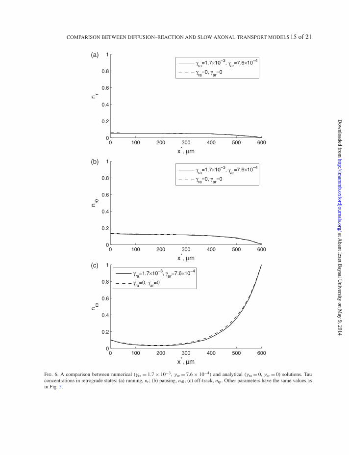
This resulted in the following values of γ s, which gave the best agreement with the tau distributionsreported in Black et al. (1996): γ ∗

01 = 4.10 × 10−2 s−1, γ ∗10 = 9.30 × 10−2 s−1, γ ∗

on = 2.75 × 10−4 s−1,γ ∗

off = 4.45 × 10−6 s−1, γ ∗ra = 6.90 × 10−5 s−1 and γ ∗

ar = 3.10 × 10−5 s−1. The main distinction fromthe set of kinetic constants given in Li et al. (2012) is that the value of γ ∗

off had to be reduced to matchthe profile reported in Black et al. (1996). Smaller γ ∗

off implies a lesser rate of tau transition from thepausing to the off-track states. We also used nx=0 = 0.1. We called the above set of γ s ‘the optimal set’.

at Abant Izzet B


ay 9, 2014http://im

amm


ownloaded from



The corresponding dimensionless values of the last two γ s in the optimal set are γra = 1.68 × 10−3 andγar = 7.56 × 10−4.

5.4 Analytical solution for slow axonal transport model

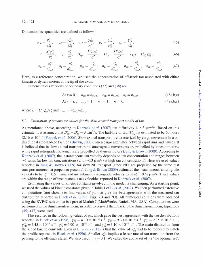
5.4.1 Simplified model Equations (39)–(44) are too complicated to obtain an analytical solution.Because reversals require switching between the type of motor that propels transport (kinesin anddynein), it is expected that reversals will be relatively infrequent, which is manifested by the smallvalues of kinetic constants that control the rates of reversals, γra and γar. We compared numerical solu-tions of Equations (39)–(44) for the optimal set of parameters with the solutions for the modified setof parameters, in which values of γra and γar were set to zero (Figs 5 and 6). The dashed lines in thesefigures correspond to γra = γar = 0. This is the case for which the analytical solution, presented in thenext section, was obtained. The solid lines correspond to γra = 1.68 × 10−3 and γar = 7.56 × 10−4. Thelength of axon was 600 µm. Values of all other parameters are from Section 5.3; dimensionless param-eter values are summarized in the caption of Fig. 5. The results for six tau populations presented inFigs. 5 and 6 suggest that γ ∗

ra and γ ∗ar can be set to zero without a significant loss of accuracy. Physically,

this is equivalent to the assumption that anterograde and retrograde populations of tau proteins remainfixed, although tau can still transition between off-track, pausing and on-track kinetic states. This meansthat, in the simplified model used for obtaining the analytical solution, the change of motors that propeltau proteins (either actual attachment/detachment of motors or possibly their activation/deactivation)can occur only at the axon hillock and the axon tip. The kinetic processes that are retained in the simpli-fied model are shown by thick arrows in Fig. 1(d). Using the approach developed in Zadeh & Montas(2010) we numerically investigated the relative sensitivities of the solutions of Equations (39)–(44) tochanges in the other four kinetic parameters, γ ∗

on, γ ∗off, γ ∗

01 and γ ∗10 (results not shown). We found that

the solutions are much less sensitive to γ ∗ra and γ ∗

ar than to the other four kinetic parameters. Setting γ ∗ra

and γ ∗ar to zero dramatically simplified Equations (39)–(44) and made it possible to obtain an analytical

solution of these equations.The simplified set of Equations (39)–(44) is

− dna

dx− γ10na + na0 = 0, (50)

vrdnr

dx− γ10nr + nr0 = 0, (51)

− (1 + γoff) na0 + γ10na + γonnap = 0, (52)

− (1 + γoff) nr0 + γ10nr + γonnrp = 0, (53)

Dapd2nap

dx2+ γoffna0 − γonnap − nap ln (2)

T1/2= 0, (54)

Drpd2nrp

dx2+ γoffnr0 − γonnrp − nrp ln (2)

T1/2= 0. (55)

5.4.2 Analytical solution for nap, na and na0 Equation (52) was solved for na0:

na0 = naγ10 + napγon

1 + γoff. (56)

at Abant Izzet B


ay 9, 2014http://im

amm


ownloaded from



0 100 200 300 400 500 6000

0.2

0.4

0.6

0.8

1

x*, μm

n a

(a)

γra

=1.7×10−3, γar

=7.6×10−4

γra

=0, γar

=0

0 100 200 300 400 500 6000

0.2

0.4

0.6

0.8

1

x*, μm

n a0

(b)

γra

=1.7×10−3, γar

=7.6×10−4

γra

=0, γar

=0

0 100 200 300 400 500 6000

0.2

0.4

0.6

0.8

1

x*, μm

n ap

(c)

γra

=1.7×10−3, γar

=7.6×10−4

γra

=0, γar

=0

Fig. 5. A comparison between numerical (γra = 1.7 × 10−3, γar = 7.6 × 10−4) and analytical (γra = 0, γar = 0) solutions. Tauconcentrations in anterograde states: (a) running, na; (b) pausing, na0; (c) off-track, nap. Dimensionless values of other parame-ters are: vr = 1.02, γ10 = 2.27, γon = 6.71 × 10−3, γoff = 1.09 × 10−4, Dap = 0.4729, Drp = 0.4729, T1/2 = 8856, L = 48.24 andnx=0 = 0.1; these correspond to dimensional parameter values discussed in section 5.3.

at Abant Izzet B


ay 9, 2014http://im

amm


ownloaded from



0 100 200 300 400 500 6000

0.2

0.4

0.6

0.8

1

x*, μm

n r

(a)

γra

=1.7×10−3, γar

=7.6×10−4

γra

=0, γar

=0

0 100 200 300 400 500 6000

0.2

0.4

0.6

0.8

1

x*, μm

n r0

(b)

γra

=1.7×10−3, γar

=7.6×10−4

γra

=0, γar

=0

0 100 200 300 400 500 6000

0.2

0.4

0.6

0.8

1

x*, μm

n rp

(c)

γra

=1.7×10−3, γar

=7.6×10−4

γra

=0, γar

=0

Fig. 6. A comparison between numerical (γra = 1.7 × 10−3, γar = 7.6 × 10−4) and analytical (γra = 0, γar = 0) solutions. Tauconcentrations in retrograde states: (a) running, nr; (b) pausing, nr0; (c) off-track, nrp. Other parameters have the same values asin Fig. 5.

at Abant Izzet B


ay 9, 2014http://im

amm


ownloaded from



Equation (56) was used to eliminate na0 from Equations (50) and (54). This resulted in the followingequations for nap and na:

(1 + γoff)dna

dx+ γ10γoffna − γonnap = 0, (57)

Dapd2nap

dx2+

(γoffγon

1 + γoff− γon − ln (2)

T1/2

)nap + γ10γoff

1 + γoffna = 0. (58)

Next na was eliminated from Equations (57) and (58) (this is similar to the approach suggested inKuznetsov, 2011). The following equation for nap was obtained:

Dapd3nap

dx3+ Dap

γoffγ10

1 + γoff

d2nap

dx2−

(γon

1 + γoff+ ln (2)

T1/2

)dnap

dx− γ10γoff

1 + γoff

ln (2)

T1/2nap = 0. (59)

The general solution of Equation (59) is

nap = c1 exp (μ1x) + c2 exp (μ2x) + c3 exp (μ3x) , (60)

where μ1, μ2 and μ3 are the roots of

Dapμ3 + Dap

γoffγ10

1 + γoffμ2 −

(γon

1 + γoff+ ln (2)

T1/2

)μ − γ10γoff

1 + γoff

ln (2)

T1/2= 0. (61)

Constants c1, c2 and c3 in Equation (60) are found from boundary conditions given by Equations (48a)and (49a) and the following boundary condition that is obtained by eliminating na from Equation (48c):

At x = 0 : Dapd2nap

dx2−

(γon

1 + γoff+ ln (2)

T1/2

)nap + γ10γoff

1 + γoffnx=0 = 0. (62)

One now obtains na by integrating Equation (57) subject to boundary condition (48c). The result is givenby Equation (A1) in the Appendix. One then finds na0 from Equation (56).

5.4.3 Analytical solution for nrp, nr, and nr0 Equation (53) was solved for nr0:

nr0 = nrγ10 + nrpγon

1 + γoff. (63)

Equation (63) was used to eliminate nr0 from Equations (51) and (55). This resulted in the followingequations for nrp and nr

vr (1 + γoff)dnr

dx− γ10γoffnr + γonnrp = 0, (64)

Drpd2nrp

dx2+

(γoffγon

1 + γoff− γon − ln (2)

T1/2

)nrp + γ10γoff

1 + γoffnr = 0. (65)

at Abant Izzet B


ay 9, 2014http://im

amm


ownloaded from



The elimination of nr from Equations (64) and (65) resulted in

Drpvrd3nrp

dx3− Drp

γoffγ10

1 + γoff

d2nrp

dx2− vr

(γon

1 + γoff+ ln (2)

T1/2

)dnrp

dx+ γ10γoff

1 + γoff

ln (2)

T1/2nrp = 0. (66)

The general solution of Equation (66) is

nrp = d1 exp (λ1x) + d2 exp (λ2x) + d3 exp (λ3x) , (67)

where λ1, λ2 and λ3 are the roots of

Drpvrλ3 − Drp

γoffγ10

1 + γoffλ2 − vr

(γon

1 + γoff+ ln (2)

T1/2

)λ + γ10γoff

1 + γoff

ln (2)

T1/2= 0. (68)

Constants d1, d2 and d3 in Equation (67) are found from boundary conditions given by Equations (48b)and (49b) and the following boundary condition that is obtained by eliminating nr from Equation (49c):

At x = L : Drpd2nrp

dx2−

(γon

1 + γoff+ ln (2)

T1/2

)nrp = 0. (69)

One now obtains nr by integrating Equation (64) subject to boundary condition (49c). The result is givenby Equation (A2) in the Appendix. One then finds nr0 from Equation (63).

The above analytical solution can be utilized to calculate the dimensionless total concentration of tauproteins and the dimensionless total flux of tau by implementing the following equations, respectively:

ntot = na + nr + na0 + nr0 + nap + nrp, (70)

jtot = −Dap∂nap

∂x− Drp

∂nrp

∂x+ na − vrnr, (71)

where

ntot = n∗tot

n∗x=L

, jtot = j∗tot

v∗an∗

x=L. (72)

Since v∗a is used as a velocity scale [see Equation (46)], the coefficient before na in Equation (71) is

equal to 1. The average velocity is still defined by Equation (15). Since the total flux of tau [Equation(71)] now has both diffusion-driven and motor-driven components, both of these components contributeto the average tau velocity.

5.5 Comparison of theory with experimental data

In Fig. 7(a), the total tau concentration obtained from either numerical (solid line) or analytical (dashedline) solutions fits well the experimental results from Figs. 7B and 7D of Black et al. (1996), whichwere normalized by using the condition ntot|x=0 = 1. To show experimental data from both Figs. 7B and7D of Black et al. (1996) such that they can be compared, results from Fig. 7B of Black et al. (1996)were stretched from 350 to 600 µm.

The flux of tau is positive, directed towards the axon tip (Fig. 7(b)). The flux is not constant, butdecreases slightly with x∗. This is due to the protein degradation described by the last two terms on theright-hand side of Equations (33) and (34).

at Abant Izzet B


ay 9, 2014http://im

amm


ownloaded from



0 100 200 300 400 500 6000

0.5

1

1.5

2

2.5

3

3.5

x*, μm

n tot

(a)γra

=1.7×10−3, γar

=7.6×10−4

γra

=0, γar

=0

data from Fig. 7B of Black et al.data from Fig. 7D of Black et al.

0 100 200 300 400 500 6000

0.005

0.01

0.015

0.02

0.025

0.03

x*, μm

j tot

(b)

γra

=1.7×10−3, γar

=7.6×10−4

γra

=0, γar

=0

0 100 200 300 400 500 6000

0.005

0.01

0.015

0.02

0.025

x*, μm

v av*, μ

m/s

(c)

γra

=1.7×10−3, γar

=7.6×10−4

γra

=0, γar

=0

Fig. 7. Numerical (γra = 1.7 × 10−3, γar = 7.6 × 10−4) and analytical (γra = 0, γar = 0) results. (a) The total concentration oftau protein in all six kinetic states. This figure also shows experimental data from Figs. 7B and 7D of Black et al. (1996).Experimental data were normalized such that at the axon hillock, x∗ = 0, ntot was equal to 1; data from Fig. 7B of Black et al.(1996) were stretched over 600 µm. (b) The total dimensionless flux of tau. (c) The average dimensional velocity of tau transport.Other parameters have the same values as in Fig. 5.

at Abant Izzet B


ay 9, 2014http://im

amm


ownloaded from



In order to explain why the slow axonal transport model with constant kinetic rates correctly capturesthe experimentally observed increase of the total tau concentration (Fig. 7(a)) while simultaneouslyshowing the positive flux of tau (Fig. 7(b)), we revisit Figs 5 and 6. The concentrations of off-track tau(Figs 5(c) and 6(c)) suggest that the diffusion-driven flux is negative in most of the axon. However, it iscounteracted by a larger positive motor-driven flux due to anterogradely running tau (Fig. 5(a)).

We again used Equation (15) to define the average velocity of tau transport. The average velocitythat follows from the slow axonal transport model (Fig. 7(c)) is larger than the average velocity thatfollows from the diffusion–reaction model (Figs 2(b,d) and 3(b,d)) and is in the range observed inexperiments (0.001–0.08 µm/s; see Konzack et al. (2007)).

6. Conclusions

We tested the performance of the diffusion–reaction and slow axonal transport models in predicting thedistribution of tau protein in axons. The models have to predict two experimentally observed features:the increase in the total tau concentration towards the growth cone and positive flux of tau towards thegrowth cone. Since tau diffusivity is positive (Konzack et al., 2007; Weissmann et al., 2009), tau cannotbe transported from the location with a low concentration (the axon hillock) to the location with a highconcentration (the axon tip) by diffusion alone, without relying on an additional physical mechanism.

We established that in order to predict these features correctly, the rate of tau attachment to MTsin the diffusion–reaction model must heavily depend on x∗, exhibiting exponential-type dependence.Location-dependent regulation of tau binding to MTs may be one way of achieving a high tau concen-tration at the axon tip. We also established that the slow axonal transport model predicts the above twofeatures even with constant kinetic rates. This is because the diffusion–reaction model totally relies onthe diffusion mechanism of tau transport to deliver tau to the growth cone. The slow axonal transportmodel, on the contrary, has two transport mechanisms, the diffusion-driven and motor-driven, and themotor-driven mechanism requires an energy input. Even if diffusion transports tau away from the axontip, motor-driven transport towards the axon tip can still be larger, thus directing the total flux of tautowards the growth cone.

The average transport velocity of tau predicted by both models is within the experimental range.However, the slow axonal transport model predicts a larger velocity, and it is expected that, for longeraxons, the reliance on motor-driven transport would be essential to sustain a sufficient flux of tau towardthe growth cone.

Acknowledgements

The authors are indebted to the anonymous reviewers for their constructive comments. A.V.K. gratefullyacknowledges the support of the Alexander von Humboldt Foundation through the Humboldt ResearchAward.

References

Baas, P., Nadar, C. & Myers, K. (2006) Axonal transport of microtubules: the long and short of it. Traffic, 7,490–498.

Black, M. M., Slaughter, T., Moshiach, S., Obrocka, M. & Fischer, I. (1996) Tau is enriched on dynamicmicrotubules in the distal region of growing axons. J. Neurosc., 16, 3601–3619.

Brown, A. (2000) Slow axonal transport: stop and go traffic in the axon. Nat. Rev. Mol. Cell Biol., 1, 153–156.

at Abant Izzet B


ay 9, 2014http://im

amm


ownloaded from



Conde, C. & Caceres, A. (2009) Microtubule assembly, organization and dynamics in axons and dendrites. Nat.Rev. Neurosci., 10, 319–332.

Cuchillo-Ibanez, I., Seereeram, A., Byers, H. L., Leung, K., Ward, M. A., Anderton, B. H. & Hanger, D.P. (2008) Phosphorylation of tau regulates its axonal transport by controlling its binding to kinesin. Faseb J.,22, 3186–3195.

Gauthier-Kemper, A., Weissmann, C., Golovyashkina, N., Seboe-Lemke, Z., Drewes, G., Gerke, V.,Heinisch, J. J. & Brandt, R. (2011) The frontotemporal dementia mutation R406W blocks tau’s interac-tion with the membrane in an annexin A2-dependent manner. J. Cell Biol., 192, 647–661.

Hinrichs, M. H., Jalal, A., Brenner, B., Mandelkow, E., Kumar, S. & Scholz, T. (2012) Tau protein diffusesalong the microtubule lattice. J. Biol. Chem., 287, 38559–38568.

Jung, P. & Brown, A. (2009) Modeling the slowing of neurofilament transport along the mouse sciatic nerve.Phys. Biol., 6, 046002.

Kanai, Y. & Hirokawa, N. (1995) Sorting mechanisms of tau and Map2 in neurons—suppressed axonal transit ofMap2 and locally regulated microtubule-binding. Neuron, 14, 421–432.

Kierszenbaum, A. (2000) The 26S proteasome: ubiquitin-mediated proteolysis in the tunnel. Mol. Reprod. Dev.,57, 109–110.

Konzack, S., Thies, E., Marx, A., Mandelkow, E. & Mandelkow, E. (2007) Swimming against the tide: mobil-ity of the microtubule-associated protein tau in neurons. J. Neurosci., 27, 9916–9927.

Kuznetsov, A. V. (2011) Analytical solution of equations describing slow axonal transport based on the stop-and-go hypothesis. Central Eur. J. Phys., 9, 662–673.

Kuznetsov, A. V. (2012) An exact solution describing slow axonal transport of cytoskeletal elements: effect of afinite half-life. Proc. R Soc. A-Math. Phys. Eng. Sci., 468, 3384–3397.

Kuznetsov, A. V., Avramenko, A. A. & Blinov, D. G. (2009) Effect of protein degradation in the axon on thespeed of the bell-shaped concentration wave in slow axonal transport. Internat. Commun. Heat Mass Transfer,36, 641–645.

Kuznetsov, A. V., Avramenko, A. A. & Blinov, D. G. (2010) Effect of diffusion on slowing the velocity of abell-shaped wave in slow axonal transport. Internat. Commun. Heat Mass Transfer, 37, 770–774.

Kuznetsov, A. V., Avramenko, A. A. & Blinov, D. G. (2011) Effect of cytoskeletal element degradation onmerging of concentration waves in slow axonal transport. Central Eur. J. Phys., 9, 898–908.

Li, Y., Jung, P. & Brown, A. (2012) Axonal transport of neurofilaments: a single population of intermittentlymoving polymers. J. Neurosci., 32, 746–758.

Li, X., Kumar, Y., Zempel, H., Mandelkow, E., Biernat, J. & Mandelkow, E. (2011) Novel diffusion barrierfor axonal retention of tau in neurons and its failure in neurodegeneration. Embo J., 30, 4825–4837.

Mandell, J. & Banker, G. (1996) A spatial gradient of tau protein phosphorylation in nascent axons. J. Neurosci.,16, 5727–5740.

Mercken, M., Fischer, I., Kosik, K. & Nixon, R. (1995) Three distinct axonal transport rates for tau, tubulin, andother microtubule-associated proteins: Evidence for dynamic interactions of tau with microtubules in vivo. J.Neurosci., 15, 8259–8267.

Peter, S. J. & Mofrad, M. R. K. (2012) Computational modeling of axonal microtubule bundles under tension.Biophys. J., 102, 749–757.

Petrucelli, L., Dickson, D., Kehoe, K., Taylor, J., Snyder, H., Grover, A., De Lucia, M., McGowan, E.,Lewis, J., Prihar, G., Kim, J., Dillmann, W., Browne, S., Hall, A., Voellmy, R., Tsuboi, Y., Dawson,T., Wolozin, B., Hardy, J. & Hutton, M. (2004) CHIP and Hsp70 regulate tau ubiquitination, degradationand aggregation. Hum. Mol. Genet., 13, 703–714.

Poppek, D., Keck, S., Ermak, G., Jung, T., Stolzing, A., Ullrich, O., Davies, K. J. A. & Grune, T. (2006)Phosphorylation inhibits turnover of the tau protein by the proteasome: influence of RCAN1 and oxidativestress. Biochem. J., 400, 511–520.

Saha, A., Hill, J., Utton, M., Asuni, A., Ackerley, S., Grierson, A., Miller, C., Davies, A., Buchman, V.,Anderton, B. & Hanger, D. (2004) Parkinson’s disease alpha-synuclein mutations exhibit defective axonaltransport in cultured neurons. J. Cell Sci., 117, 1017–1024.

at Abant Izzet B


ay 9, 2014http://im

amm


ownloaded from



Samsonov, A., Yu, J. Z., Rasenick, M. & Popov, S.V. (2004) Tau interaction with microtubuies in vivo. J. CellSci., 117, 6129–6141.

Stamer, K., Vogel, R., Thies, E., Mandelkow, E. & Mandelkow, E. (2002) Tau blocks traffic of organelles,neurofilaments, and APP vesicles in neurons and enhances oxidative stress. J. Cell Biol., 156, 1051–1063.

Utton, M., Connell, J., Asuni, A., van Slegtenhorst, M., Hutton, M., de Silva, R., Lees, A., Miller, C. &Anderton, B. (2002) The slow axonal transport of the microtubule-associated protein tau and the transportrates of different isoforms and mutants in cultured neurons. J. Neurosc., 22, 6394-6400.

Utton, M., Noble, W., Hill, J., Anderton, B. & Hanger, D. (2005) Molecular motors implicated in the axonaltransport of tau and alpha-synuclein. J. Cell Sci., 118, 4645–4654.

Wang, L. & Brown, A. (2002) Rapid movement of microtubules in axons. Curr. Biol., 12, 1496–1501.Weissmann, C., Reyher, H., Gauthier, A., Steinhoff, H., Junge, W. & Brandt, R. (2009) Microtubule binding

and trapping at the tip of neurites regulate tau motion in living neurons. Traffic, 10, 1655–1668.Zadeh, K. S. & Montas, H. J. (2010) A class of exact solutions for biomacromolecule diffusion–reaction in live

cells. J. Theoret. Biol., 264, 914–933.

Appendix

The analytical solution for na, obtained by integrating Equation (57) subject to boundary condition (48c)and using Equation (60), is

na(x) =(

exp

[− γ10γoff

1 + γoffx

] (nx=0(µ1 + γoff(γ10 + µ1))(µ2 + γoff(γ10 + µ2))(µ3 + γoff(γ10 + µ3))

+ γon

(c1

(−1 + exp

[(γ10γoff

1 + γoff+ µ1

)x

])(µ2 + γoff(γ10 + µ2))(µ3 + γoff(γ10 + µ3))

+ (µ1 + γoff(γ10 + µ1))

(c3

(−1 + exp

[(γ10γoff

1 + γoff+ µ3

)x

])(µ2 + γoff(γ10 + µ2))

+(

c2

(−1 + exp

[(γ10γoff

1 + γoff+ µ2

)x

])(µ3 + γoff(γ10 + µ3))

))))

/((µ1 + γoff(γ10 + µ1))(µ2 + γoff(γ10 + µ2))(µ3 + γoff(γ10 + µ3))) (A.1)

while the analytical solution for nr, obtained by integrating Equation (64) subject to boundary condition(49c) and using Equation (67), is

nr(x) =(

exp

[− γ10γoff

vr(1 + γoff)L

]γon

(−d1

(exp

[γ10γoff

vr(1 + γoff)x + λ1L

]− exp

[γ10γoff

vr(1 + γoff)L + λ1x

])

× (γ10γoff − vr(1 + γoff)λ2)(γ10γoff − vr(1 + γoff)λ3) − (γ10γoff − vr(1 + γoff)λ1)

×(

d3

(exp

[γ10γoff


]− exp

[γ10γoff


])(γ10γoff − vr(1 + γoff)λ2)

+d2

(exp

[γ10γoff


]− exp

[γ10γoff


])(γ10γoff − vr(1 + γoff)λ3)

)))

/((γ10γoff − vr(1 + γoff)λ1)(γ10γoff − vr(1 + γoff)λ2)(γ10γoff − vr(1 + γoff)λ3)). (A.2)

at Abant Izzet B


ay 9, 2014http://im

amm


ownloaded from


Documents

A comparison between the diffusion-reaction and slow axonal transport models for predicting tau distribution along an axon