A Comparative Study of Techniques for Energy ... - hcl.ucd.ie

Received July 11, 2020, accepted July 29, 2020, date of publication August 3, 2020, date of current version August 17, 2020.

Digital Object Identifier 10.1109/ACCESS.2020.3013812

A Comparative Study of Techniques for EnergyPredictive Modeling Using PerformanceMonitoring Counters on ModernMulticore CPUsARSALAN SHAHID , MUHAMMAD FAHAD , RAVI REDDY MANUMACHU ,AND ALEXEY LASTOVETSKYSchool of Computer Science, University College Dublin, Dublin 4, D04 V1W8 Ireland

Corresponding author: Arsalan Shahid ([email protected])

This work was supported by the Science Foundation Ireland (SFI) under Grant 14/IA/2474.

ABSTRACT Accurate and reliablemeasurement of energy consumption is essential to energy optimization atan application level. Energy predictive modelling using performance monitoring counters (PMCs) emergedas a promising approach, one of the main drivers being its capacity to provide fine-grained component-levelbreakdown of energy consumption. In this work, we compare two types of energy predictive modelsconstructed from the same set of experimental data and at two levels, platform and application. The firsttype contains linear regression (LR) models employing PMCs selected using a theoretical model of energyof computing. The second type contains sophisticated statistical learning models, random forest (RF)and neural network (NN), that are based on PMCs selected using correlation and principal componentanalysis. Our experimental results performed on two modern Intel multicore processors using a diverse setof applications and a wide range of application configurations, show that the average proportional predictionaccuracy of platform-level LR models is 5.09× and 4.37× times better than the platform-level RF andNN models. We also present an experimental methodology to select a reliable subset of four PMCs forconstructing accurate application-specific online models. Using the methodology, we demonstrate that LRmodels perform 1.57× and 1.74× times better than RF and NN models. The consistent accuracy of LRmodels stress the importance of taking into account domain-specific knowledge for model variable selection,in this case, the physical significance of the PMCs originating from the conservation of energy of computing.The results also endorse the guidelines of the theory of energy of computing, which states that any non-linearenergy model (in this case, the RF and NN models) employing PMCs only, will be inconsistent and henceinherently inaccurate.

INDEX TERMS Energy predictive modelling, energy additivity, linear regression, neural networks, randomforest, matrix multiplication, fast Fourier transform.

I. INTRODUCTIONEnergy of computing is a key environmental concernand optimizing it has become a principal technologi-cal challenge. Information and Communications Technol-ogy (ICT) systems and frameworks are currently utilizingabout 2000 terawatt-hours (TWh) per year that representabout 10% of the worldwide electricity demand [1].Andrae and Edler [2] predict that computing systems and

The associate editor coordinating the review of this manuscript and

approving it for publication was Shadi Alawneh .

devices will consume up to 50% of global electricityin 2030with a contribution towards greenhouse gas emissionsof 23%.

Energy optimization in computing is driven by inno-vative developments both at system-level and application-level. System-level optimization strategies [3]–[9] target toimprove the energy efficiency of the overall execution envi-ronment of applications using methods including DynamicVoltage and Frequency Scaling (DVFS), Dynamic PowerManagement (DPM) and energy-aware task scheduling.Application-level optimization strategies [10]–[14] consider

143306 This work is licensed under a Creative Commons Attribution 4.0 License. For more information, see https://creativecommons.org/licenses/by/4.0/ VOLUME 8, 2020

https://orcid.org/0000-0002-3748-6361

https://orcid.org/0000-0002-3595-8484

https://orcid.org/0000-0001-9181-3290

https://orcid.org/0000-0001-9460-3897

https://orcid.org/0000-0002-3360-9440

A. Shahid et al.: Comparative Study of Techniques for Energy Predictive Modeling Using PMCs on Modern Multicore CPUs

FIGURE 1. Number of research publications on computing energy using PMCs and in other areas ofenergy in computing including frequency scaling, dynamic voltage scaling, power usageeffectiveness, energy proportional computing, and energy-efficient ethernet. The number ofpublications addressing PMC based energy modelling increase by 4.5×. These statistics have beencollected from Google Scholar and Microsoft Academic.

the application-level parameters as model variables in ana-lytic models to improve the energy efficiency of theapplications.

Accurately measuring the energy consumption during theexecution of an application is vital for energy optimiza-tion methods at the software level. The three mainstreamapproaches for energy consumption measurement include:(a) External power meter based system-level measurements,(b) use of on-chip voltage and current sensors, and (c) pre-dictive models using application and system characteristicsas model variables. Fahad et al. [15] present a comprehen-sive study of the three mainstream approaches to providinga measurement of energy consumption during applicationexecution. An overview of the three methods is presented inthe related work. Briefly, power meters based system-levelphysical measurements are reliable, accurate, and is consid-ered the ground truth. The profiles obtained for the dynamicenergy consumption of the applications using on-chip sen-sors exceptionally diverge from the ones obtained using theground truth. This discovery suggested that the use of on-chipsensors based measurements do not capture the full sketch ofthe dynamic energy consumption during an application run.

Energy predictive models using performance monitoringcounters (PMCs) emerged as a promising energy measure-ment approach because of its ability to provide a fine-grainedcomponent-level breakdown of energy consumption. PMCsare special-purpose hardware registers provided in modernprocessor architectures to record the counts of softwareevents, that represent the kernel-level activities such as page-faults, context-switches, etc., and hardware events arising

from the micro-architecture core and the performance moni-toring unit (PMU) such as CPU-cycles, branch-instructions,cache-misses, etc. Figure 1 graphs the number of academicpublications over the years in the field of energy of computingand shows that energy predictive modelling using perfor-mance events has become a dominant research topic.

Modern multicore CPUs deliver a vast set of PMCs. How-ever, the system users can obtain a limited number of PMCs(typically 3-4 at a time) for an application execution becauseof the little number of hardware registers devoted to recordthem. Let us consider the Intel Haswell server (specificationin Table 1). On this platform, the Likwid tool [16] exposes167 PMCs. An application must be run about 53 timesto collect the values of all the representative PMCs. Sinceonly 3-4 PMCs can be collected in a single application run,immense programmingwork and time are needed to automateand record all the PMCs. Therefore, selecting a reliable subsetof PMCs is crucial to the construction and prediction accuracyof the energy predictive models. We now summarize themainstream approaches for selecting the PMCs:• Approaches that take into account all the PMCs providedby a framework or tool for a platform for a given appli-cation with the aim to record all the activities that areviable contributors to energy consumption. Due to thehigh complexity of this approach, we did not find anyresearch works adopting it.

• Approaches that are based on a statistical methodol-ogy for feature selection and feature extraction suchas correlation, principal component analysis (PCA),etc. [17], [18].

VOLUME 8, 2020 143307


TABLE 1. Specification of the Intel Haswell (HCLServer1) and Intel Skylake (HCLServer2) multicore CPU Server.

• Approaches that take into account the expert advice orintuition to select a possibly reliable subset (that may notbe exploited in one application run), which, in experts’opinion, is a dominant contributor to energy consump-tion [19].

• Approaches that select PMCs using a theoretical modelof the energy of computing, which is the manifestationof the fundamental physical law of energy conservation.[20], [21].

The theory of energy of computing has progressivelymatured over the past three years starting with a proposal ofa criterion for selection of PMCs in the research work [20]followed by a formal description of the theory and its practicalimplications in [21]. Shahid et al. [20] propose a novel prop-erty of PMCs called additivity, which is true for all PMCs,whose count for the serial executions of two applications isequal to the sum of counts for the sole execution of eachapplication. The authors study the additivity of PMCs pro-vided by the two mainstream frameworks, Likwid [16] andPAPI [22] on amodern Intel Haswell multicore server. Energyadditivity is based on an experimental observation that theenergy consumption of the serial execution of two or moreapplications is equal to the sum of the energy consumption ofthe individual applications. If a PMC is employed as a modelvariable in an energy predictive model, its must follow therule of additivity. The authors further demonstrate that manyPMCs available on modern processors obtained using Likwidand PAPI that are extensively used in models as crucial model

variables are non-additive. Shahid et al. [21] proposed anovel theory of energy of computing and unified its practicalimplications to increase the prediction accuracy of linearenergy predictivemodels in a consistency test, which containsa suite of properties that include determinism, reproducibility,and additivity to select model variables and constraints formodel coefficients. The authors show that failure to satisfythe requirements of the test worsens the prediction accuracyof linear energy predictive models.

In this work, we compare two types of energy predictivemodels constructed from the same set of experimental dataand at two levels, platform and application. The first typecontains linear regression (LR) models employing PMCsselected using the theoretical model of the energy of com-puting. The second type has sophisticated statistical learningmodels, random forest (RF), and neural network (NN), thatare based on PMCs selected using correlation and principalcomponent analysis.

We divide the experiments in this article into two maingroups: Group 1 and Group 2. In Group 1, we experimentallycompare the prediction accuracy of platform-level energypredictive models on HCLServer1 (Table 1). The models areanalyzed in two configurations. In the first configuration,the models are trained and tested using datasets that containall the applications. In the second configuration, the dataset ofapplications is split into two datasets, one for training modelsand the other for testing models. We demonstrate that LRmodels exhibit better prediction accuracies than RF and NN

143308 VOLUME 8, 2020


models in both the configurations (5.09× and 4.37× timesspecifically for the first configuration).

In Group 2, we examine the accuracy of application-specific energy predictive models. The experiments in thisgroup are performed on HCLServer2 (Table 1) and containmodels of the two types. We choose two well-known andhighly optimized scientific kernels offered by the Intel MathKernel Library (MKL), 2D fast Fourier transform (FFT) anddense matrix multiplication (DGEMM). We select a set ofnine most additive PMCs (PA) and a set of nine PMCs thatare non-additive (PNA) that are common for both the appli-cations. PNA belongs to the dominant PMC groups reflect-ing the energy-consuming activities and has been widelyemployed in the models found in the literature (Section III).We build LR models employing PA and PNA. We demon-strate that the models based on PA have better predictionaccuracy than the models based on PNA. To build onlineenergy predictive models based on four PMCs, we composetwo subsets of PMCs, PA4 and PNA4 from PA and PNA, con-taining four PMCs highly positively correlated with energy.Models that use PA4 exhibit 3.44× and 1.71× better averageprediction accuracy than models using PNA4. We conclude,therefore, that a high positive correlation of model variableswith dynamic energy consumption alone is not sufficient toprovide good prediction accuracy but should be combinedwith methods such as additivity that consider the physicalsignificance of the model variables originating from the the-ory of energy conservation of computing. For the same twoapplications, we compare the LR models based on the setof four most additive and highly positively correlated PMCs(PA4) with the RF and NN models based on four PMCsselected using correlation and PCA. The results show that theLR model performs 1.57× and 1.74 × times better than RFand NN models.

Based on our experiments, we conclude that linear regres-sion models based on PMCs selected using the theoreticalmodel of the energy of computing perform better than RF andNN models using the standard statistical approaches.

To summarize, our key contribution in this work is that wepresent the first comprehensive experimental study compar-ing linear regression models employing PMCs selected usinga theoretical model of the energy of computing with sophis-ticated statistical learning models, random forest and neuralnetwork, that are constructed using PMCs selected based oncorrelation and principal component analysis. We show thatthe LR models perform better than the RF and NN modelsthereby highlighting two important points. First, the consis-tent accuracy of LRmodels highlight the importance of takinginto account domain-specific knowledge for model variableselection, in this case, the physical significance of the PMCsoriginating from the conservation of energy of computing.Second, according to the theory of energy of computing,any non-linear energy model (in this case, the RF and NNmodels) employing PMCs onlywill be inconsistent and henceinherently inaccurate. A non-linear energy model, in order

to be accurate, must employ non-additive model variables inaddition to PMCs.

The rest of this article is organized as follows. Section 2presents the terminology. Section 3 highlights the relatedwork followed by the practical implications of the theoryof energy of computing in Section 4. Section 5 presentsour experimental setup including the platform and applica-tion details, tools, and modelling techniques. In Section 6,we present the experimental results and discussions. Finally,Section 7 concludes the paper.

II. TERMINOLOGY RELATED TO ENERGY, PREDICTIONERROR MEASURES, AND STATISTICAL TECHNIQUESA. ENERGY CONSUMPTIONTotal energy consumption can be represented as a sum ofstatic energy and dynamic energy. We determine the staticenergy consumption by multiplying the base or idle power ofthe system (i.e., with no running application) with the appli-cation’s execution time. However, we calculate the dynamicenergy consumption (energy consumption of the application)by subtracting the static energy from the total energy utilizedby the system during the application execution. In otherwords, if PS represents the base or idle power of the system,ET is the total energy consumption of the system duringan application run for TE seconds, then the dynamic energyconsumption ED can be determined by using Equation 1.

ED = ET − (PS × TE ) (1)

The rationale backing the use of dynamic energy consump-tion rather than total energy consumption is given in theAppendix I.

B. PREDICTION ERROR MEASURESWe compare the prediction accuracy of models using twomeasures: a) Relative error, and b) Proportional error. Therelative error p of a predicted dynamic energy consumption ewith respect to the ground truth dynamic energy consumptionr is given below:

p =|r−e|r× 100 (2)

The measure p gives a lower relative error for a modelthat underestimates than a model that overestimates (forexample: when you consider the same proportion for theunderestimated and the overestimated values of e with r).This can negatively impact the interpretation of the results.Rico-Gallego et al. [23] propose the proportional error µ tocorrect the anomaly. The proportional error for model pre-diction e with the ground truth r is a ratio of a maximumof the two values with the minimum of the two values. It isrepresented by the following equation 3.

µ =max(r, e)min(r, e)

(3)

µ is always greater than 1 if there exists an error, and equalto 1 otherwise.

VOLUME 8, 2020 143309


C. MODEL VARIABLE SELECTION TECHNIQUESWe employ twomodel variable selection methods for randomforest and neural network models. They are: 1). Correlation,and 2). Principal Component Analysis (PCA).

Correlation is a statistical metric to understand the rela-tionship between two variables and is calculated using thefollowing Equation 4.

Cep =

∑(ei − e)(pi − p)√∑

(ei − e)2∑

(pi − p)2(4)

where, Cep is the correlation coefficient between the dynamicenergy consumption e and the PMC pi. ei represents energyconsumption of an application and e is the mean of the energyof all the applications in the data-set. pi is the PMC count andp is it’s mean for all the applications in the data-set. The valueof the correlation coefficient is between −1 to 1. A value of−1 forCepmeans perfect negative correlation, 0 signifying nocorrelation, and+1, a perfect correlation between the energyand the PMC.

Principal Component Analysis (PCA) [24] is applied todetermine the most statistically influential PMCs. It is amultivariate statistical technique for feature extraction and isused for dimensionality reduction in high-dimensional data.It uses a correlation matrix to ease the analysis by selectingthe most valuable features in a data-set. The top principalcomponent captures the maximum variability in the data,and each succeeding component has the highest variabilitysubject to the constraint imposing orthogonality with theprevious principal components.

III. RELATED WORKThis section presents a literature survey of mainstreamenergy measurement methods and highlights their prosand cons, dominant tools used to obtain PMCs, prominentworks towards the construction of energy predictive models,research works that provide a critical review of PMCs, andfinally, recent developments in the energy predictive modelsusing PMCs.

A. ENERGY MEASUREMENT METHODSThe three mainstream methods for energy measurement dur-ing an application execution are: (a). Power meters-basedphysical measurements at platform-level, (b). on-chip sensorsbased voltage and current measurements, and (c). Energy pre-dictivemodels using application and system characteristics asmodel variables.

The first method using the external power meters is knownto be accurate and considered as the ground truth. It hasbeen used for providing the measurements at a system-level.Fahad et al. [25] presented the first methodology (that is,AnMoHA) to measure the component-level energy consump-tion of a platform using external power meters. The authorsdemonstrate that their approach provides accurate energyconsumption decomposition up to socket-level. However,

the core-level granularity for energy consumption decompo-sition has not been achieved.

The second method used on-chip voltage and currentsensors to determine power and are now supported bypopular processor vendors such as Intel, AMD, and IBMPower CPUs, Nvidia GPUs, and Intel Xeon Phis. There arevendor-specific libraries to acquire the power data from thesesensors. For example, Running Average Power Limit (RAPL)[26] is used tomonitor power and control frequency (and volt-age) of Intel CPUs. Similarly, Nvidia NVIDIA ManagementLibrary (NVML) [27] and Intel System Management Con-troller chip (SMC) [28] provide the power consumption byNvidia GPUs and Intel Xeon Phi. NVML provides the instantpower draw values with nominal accuracy up to ±5% [27].The accuracy of Intel SMC is not available. Apart frominsufficient documentation, there are other issues with thepower data values provided by these vendor-specific libraries.For example, it lacks details such as update frequency ofpower readings and also suffers from potential complicationssuch as sampling interval variability of significant sensorlag as reported by [29]. Fahad et al. [15] present the firstdetailed study on the accuracy of on-chip power sensors andshow that deviations of the energy measurements provided byon-chip sensors from the system-level power measurements(considered as ground truth) do not motivate their use in theoptimization of applications for dynamic energy.

The third method using energy predictive models (employ-ing application and hardware parameters as model variables)emerged as a popular alternative to determine the energyconsumption of an application. It is because of the model’sability to provide fine-grained component-level (such as core-level, cache-level, etc.) energy consumption measurements.A vast number of these models are linear andmake use of per-formance monitoring counters (PMCs) as model variables.This approach forms the focus of this work.

B. TOOLS TO OBTAIN PMCsLinux Perf [30] also called perf_events can be used to gatherthe PMCs for CPUs in Linux. It also comes as a perfor-mance profiling tool suite including perf stat, perf record, perfreport, perf annotate, perf top and perf bench.Intel PCM [31] is used for reading PMCs of core and

uncore (which includes the QPI) components of an Intelprocessor. It is exposed to programmers as a C++API and isalso able to provide energy measurements from Intel on-chipsensors. It can further support the statistical analysis of corefrequencies, QPI power, and DRAM activities.

PAPI [22] provides a standard API for accessing PMCsavailable on most modern microprocessors. It provides twotypes of events, native events and present events. Nativeevents correspond to PMCs native to a platform. They formthe building blocks for present events. A preset event ismapped onto one or more native events on each hardwareplatform. While native events are specific to each platform,preset events obtained on different platforms can not becompared.

143310 VOLUME 8, 2020


Likwid [16] provides command-line tools and an API toobtain PMCs for both Intel, POWER8, and AMD proces-sors on the Linux OS. It contains a variety of performancemeasurement and application tunning tools such as likwid-pin and likwid-bench. Furthermore, Likwid is light-weight,which means the performance overheads of Likwid is lessthan 6000 cycles. The recent stable released version is Likwid5.0 with support to extract PMCs of accelerators such asGPUs.

For Nvidia GPUs, CUDA Profiling Tools Interface(CUPTI ) [32] can be used for obtaining the PMCs for CUDAapplications. CUPTI provides the following APIs: ActivityAPI, Callback API, Event API, Metric API, and Profiler API.Sample PMCs that can be obtained using these APIs are totalinstruction count, data rate, memory load, and store counts,cache hits and misses, number of branches instructions, etc.

C. NOTABLE ENERGY PREDICTIVE MODELS FOR CPUsThe concept of exploiting the utilization metrics of activecomputing resources (such as CPU, memory, disks, and I/O)has been widely adopted in dynamic power managementtechniques [33]–[35]. Some of the initial efforts towardsenergy consumption modelling correlating PMCs with powerand energy measurements include [36]–[43]. The frequentlyused parameters include integer operations, floating-pointoperations, memory requests due to cache misses, componentaccess rates, instructions per cycle (IPC), CPU/disk and net-work utilization, etc. were trusted to be highly correlated withenergy utilization. Simple linear models have been developedusing PMCs and correlated features to predict the energyconsumption of platforms. Rivoire et al. [44] and Rivoire [45]study and compare five full-system, real-time power models,using a variety of machines and benchmarks. They report thatthe PMC-based model is the best overall in terms of accuracysince it accounted for the majority of the contributors to thesystem’s dynamic power. Other notable PMC-based linearmodels are [19], [46]–[51].

Rotem et al. [26] present RAPL, in Intel Sandybridge topredict the energy consumption of core and uncore compo-nents (QPI, LLC) based on PMCs (which are not disclosed).Lastovetsky and Reddy [13] present an application-levelenergy model where the dynamic energy consumption of aprocessor is represented by a function of problem size. UnlikePMC-based models that contain hardware-related PMCs anddo not consider problem size as a variable, this model takesinto account the highly non-linear and non-convex nature ofthe relationship between energy consumption and problemsize for solving optimization problems of data-parallel appli-cations on homogeneous multicore clusters for energy.

D. NOTABLE ENERGY PREDICTIVE MODELS FORACCELERATORS AND HPC APPLICATIONSSome of the promising research contributions for theenergy predictive models on GPU accelerators using PMCsinclude [52]–[54]. PMCs counts can be recorded duringthe application run by using the CUDA Profiling Tools

Interface (CUPTI) [32]. An instruction-level energy con-sumption model for Xeon Phi processors forms the basis ofwork presented by Shao and Brooks [55]. Another linearinstruction-level model for predicting the dynamic energyconsumption on the soft processors based on FPGA waspresented by Khatib et al. [56]. Inter-instruction effects andthe operand values of the instructions have been consideredby the proposed model.

Some notable platform-wide power models for HPC ser-vers based on PMCs include [57]–[59]. Gschwandtner et al.[60] presented linear regression models based on hardwarecounters for prediction of energy consumption of HPC appli-cations executing on the IBM POWER7 processor.

E. CRITIQUES OF PMCs FOR ENERGYPREDICTIVE MODELLINGReferences [20], [41], [61]–[63] are research works that crit-ically examine the accuracy of PMC based energy predictivemodels and demonstrate their poor prediction accuracy. Theresearchers in [61] point out the fundamental limitation toobtain all the PMCs simultaneously or in a single applicationrun and argue that the linear regression models yield predic-tion errors as high as 150%.

Fahad [15] demonstrated the state-of-the-art linear energypredictive models employing PMCs that are selected usingstatistical correlations are pruned to errors because they donot consider the physical significance of model variables,coefficients, and intercepts. The authors show average errorbetween platform level PMC models using linear regressionand the ground truth (power-meters) ranges from 14% to 32%and the maximum reaches 100%.

F. RECENT DEVELOPMENTS IN THE ENERGYPREDICTIVE MODELS USING PMCsIn all previous works, the causes of the inaccuracy of energypredictive models or the reported wide variance of the accu-racy of the models have not been studied. Furthermore,a sound theoretical framework to understand the fundamentalsignificance of the model variables concerning the dynamicenergy consumption has been lacking.

The theory of energy of computing has progressivelymatured over the past three years starting with a proposal ofa criterion for selection of PMCs in the research work [20]followed by a formal description of the theory and its prac-tical implications in [21]. Shahid et al. [20] proposed anovel selection criterion for PMCs called additivity, whichcan be used to determine the set of PMCs for accurate andreliable energy predictive modelling. They experimentallydemonstrate that majority of PMCs exposed by Likwid andPAPI on a modern Intel Haswell server are non-additive.Furthermore, the authors argue that non-additive PMCs havebeen employed as key model variables for energy predic-tions thereby questioning the accuracy and reliability of suchmodels.

Shahid et al. [64] show that the accuracy of energy predic-tive models based on three popular mainstream techniques

VOLUME 8, 2020 143311


(linear regression, random forests, and neural networks) canbe improved by selecting PMCs using the property of addi-tivity. They show that the removal of non-additive PMCsimproves the average prediction accuracy of linear regressionmodels from 31% to 18%, random forest models from 38%to 24%, and neural network models from 30% to 24%.

Shahid et al. [21] further proposed a novel theory of energyof computing and unified its practical implications to increasethe prediction accuracy of linear energy predictive models ina consistency test, which contains a suite of properties thatinclude determinism, reproducibility, and additivity to selectmodel variables and constraints for model coefficients. Theauthors conducted a fundamental study showing the rise inthe number of non-additive PMCs along with the increase inthe number of cores employed during the execution of theapplications. The authors attribute the rise in the number ofnon-additive PMCs to the inherent complexities of modernmulticore platforms such as severe resource contention andnon-uniform memory access (NUMA).

IV. THEORY OF ENERGY OF COMPUTING:PRACTICAL IMPLICATIONSA theory of energy of computing has been developed overthe past three years starting with the proposal of a criterionfor selection of PMCs in the research work [20] followed bya formal description of the theory and its practical implica-tions for improving the prediction accuracy of linear energypredictive models in [21].

The theory of energy of computing is a formalism con-taining properties of PMC-based energy predictive modelsthat are manifestations of the fundamental physical law ofenergy conservation. The properties capture the essence ofsingle application runs and characterize the behavior of serialexecution of two applications. They are intuitive and experi-mentally validated and are formulated based on the followingobservations:

• In a fully dedicated and stable environment, with eachexecution of a single application being represented bythe same PMC vector, for any two applications, the PMCvector of their serial execution will always be the same.

• An application run that does not perform any work doesnot consume or generate energy. It is represented by anull PMC vector (where all the PMC values are zeroes).

• An application with a PMC vector that is not nullmust consume some energy. Since PMCs account forenergy-consuming activities of applications, an appli-cation with any energy-consuming activity higher thanzero activity must consume more energy than zero.

• Finally, the consumed energy of compound applicationis always equal to the sum of energies consumed bythe individual applications. The serial execution of twoapplications, say the base applications, forms a com-pound application.

The practical implications of the theory for constructingaccurate and reliable linear energy predictive models are

unified in a consistency test. The test includes the followingselection criteria for model variables, model intercept, andmodel coefficients:• Each model variable must be deterministic and repro-ducible. In the case of PMC-based energy predictivemodels, the multiple runs of an application keeping theoperating environment constant must return the samePMC count.

• Each model variable must be additive. The property ofadditivity is further summarized in the following section.

• The model intercept must be zero.• Each model coefficient must be positive.The first two properties are combined into a additivity test

for the selection of PMCs. A linear energy predictive modelemploying PMCs and which violates the properties of theconsistency test will have poor prediction accuracy.

By definition and intuition, PMCs are all pure countersof energy-consuming activities in modern processor archi-tectures and as such must be additive. Therefore, accordingto the theory of energy of computing, any consistent, andhence accurate, energy model, which only employs PMCs,must be linear. This also means that any non-linear energymodel employing PMCs only, will be inconsistent and henceinherently inaccurate. A non-linear energy model, in orderto be accurate, must employ non-additive model variables inaddition to PMCs.

A. Additivity OF PMCsThe property of additivity is based on an intuitive and simplerule that if a PMC is intended to be employed as a modelvariable in a linear energy predictive model, then its countfor a compound application should be equal to the sum ofits counts for the executions of the base applications formingthe compound application. It is based on the experimentalobservation and a well-known fact that the dynamic energyconsumption of a serial run of two applications is the sumof dynamic energy consumption observed for the sole execu-tions of each application.

The additivity of a PMC is determined as follows. We firstobtain the counts of the PMC for the sole executions of thebase applications. Then, we run the compound applicationand record its count of the PMC. Generally, the main com-putations for the compound application consist of the maincomputations of the base applications executed one after theother. If the PMC of the compound application is equal to thesum of the PMCs obtained for the base applications (withina tolerance of 5.0%), the PMC is categorized as potentiallyadditive. Else, it is labeled as non-additive.

For each PMC, we determine the maximum percentageerror. Since the ground truth between the sum of base appli-cations’ PMCs and the compound application PMCs is notknown, we use Equation 5 instead of Equation 2 to calculatethe percentage error for a compound application, as follows:

Error(%) = |(eb1 + eb2)− ec(eb1 + eb2 + ec)/2

| × 100 (5)

143312 VOLUME 8, 2020


TABLE 2. List of applications employed for studying the prediction accuracy of the models.

where ec, eb1, eb2 are the PMCs for the compound applica-tion and the constituent base applications respectively. Theadditivity test error for a PMC is the maximum of percentageerrors for all the compound applications in the experimentaltest-suite.

V. EXPERIMENTAL SETUPA. PLATFORM AND APPLICATIONSThe experiments are carried out on two modern multicoreplatforms: 1). Intel Haswell dual-socket server, and 2). IntelSkylake single-socket server. The specifications for both aregiven in Table 1.Our test suite (Table 2) contain a broad set of standard

benchmarks with highly memory-bound and compute-boundscientific computing applications such as DGEMM and FFTfrom Intel math kernel library (MKL), scientific applicationsfrom NAS Parallel benchmark suite, Intel HPCG, stress, andtwo unoptimized applications.

B. SOFTWARE TOOLSWe measure the following during an application exe-cution: 1). Dynamic energy consumption, 2). Executiontime, and 3). PMCs. The experimental workflow is shownin Figure 2. The dynamic energy consumption is deter-mined using system-level power measurements providedby WattsUp Pro power meter. The readings are recordedprogrammatically using a detailed statistical methodologyemploying HCLWattsUp API [65]. We periodically calibratethe power meters by using YokogawaWT210 that is an ANSIC12.20 revenue-grade power meter. We detail the usage ofHCLWattsUp API in Appendix II and experiments for cal-ibration of the power-meters are presented in Appendix V.We follow a strict statistical methodology to confirm theexperimental accuracy and reliability where a sample mean

for a response variable is obtained from several experimentalapplication runs (Appendix III).Likwid package [16] has been used to record the PMCs.

On an Intel Haswell platform, it offers 164 PMCs, whereas,385 PMCs are exposed on an Intel Skylake platform. ThePMCs with counts less than or equal to 10 have been elim-inated considering their insignificance for modelling thedynamic energy consumption since they are non-reproducibleover several executions of the same application on our plat-form.

The resultant set of PMCs contains a total of 151 for IntelHaswell and 323 for Intel Skylake. The process of collectionof all the PMCs consumes a lot of time since only fourPMCs can be recorded for one execution of an applicationreason being a small number of available hardware registersstoring them. Furthermore, many PMCs need to be recordedseparately or in sets of two or three for a single applicationrun. Therefore, to record all the PMCs, one must execute anapplication about 53 and 99 times on Intel Haswell and IntelSkylake platform, respectively.

We use a tool called AdditivityChecker (Appendix VII),that automates the determination of the additivity value of aPMC.

C. TYPES OF ENERGY PREDICTIVE MODELSThe types of energy predictive models that we compare in thiswork are described below:

• Linear Regression (LR): A LR based model can bestated as follows:

ED =n∑

k=1

βk × ek (6)

where ED is the dynamic energy consumption, β0 iscalled the model intercept, the β = {β1, . . . , βn} is thevector of regression coefficients or themodel parameters

VOLUME 8, 2020 143313


FIGURE 2. Experimental workflow to determine the PMCs for our HCLServer platforms.

and {e1, . . . , en} are the PMCs. In real life, there usu-ally is stochastic noise (measurement errors). Therefore,the measured energy is typically expressed as

ED =n∑

k=1

βk × ek + ε (7)

where the error term or noise ε is a Gaussian randomvariable with expectation zero and variance σ 2, writtenε ∼ N (0, σ 2).We build a specialized linear model usinga regression technique that constrains the regressioncoefficients (β) to be positive.

• Random Forest (RF): A RF technique is a supervisedlearning algorithm using a decision tree-based approachto train on a data-set and output mean prediction from

individual trees. It is considered for its accuracy inclassification and regression-based tasks [66]. It is anon-linear machine learning model build by construct-ing many linear boundaries. The overall non-linearityis because a single linear function can not be used toclassify and regress on each iteration of the decision tree.

• Neural Networks (NN): A NN model is inspired byneurons of a human brain and contains an interconnectedgroup of nodes where each node computes weights andbiases and give an output prediction. We set the trans-fer/activation function as linear. The learning functionis Bayesian regularization that gives optimal regulariza-tion parameters in an automated fashion [67]. Bayesianregularization updates the weight and biases by using

143314 VOLUME 8, 2020


FIGURE 3. Model training and testing pipelines for LR, RF, and NN models.

the Levenberg-Marquardt algorithm [68], which is usedto train the NN up to 100 times quicker in com-parison with the commonly used gradient-descent andback-propagation method.

The training parameters employed to build the models aregiven in Table 3. Figure 3 explains the machine learningmodel pipeline. It has four main stages: 1). Data collection,2). PMC selection, 3). Model training, and 4). Model test-ing or validation. After the collection of the data-set fromHCLServers, the data is passed through a PMC selectionstage which first normalizes the PMC counts. To constructthe LR models, PMCs are first checked for their additivityusing the Additivity Test, and the topmost additive PMCsare selected as model variables. To build the RF and NNmodels, the PMCs are first evaluated based on their statisticalcorrelation. The set of top positively correlated PMCs is thenfurther pruned using PCA. The correlation and PCAmethodsare explained in detail in the section VI-2. The set of selectedPMCs is then split into two subsets. One for training themodels and the other for testing their accuracy.

D. SELECTION METHODS FOR PMCsWe now summarize the steps to select model variables orPMCs using two approaches as described below:

TABLE 3. Modelling Parameters.

1) PMCs are selected based on the consistency test fromthe theory of energy of computing (Section IV) andemployed as model variables in linear regression (LR)models. The steps for the PMC selection include:

VOLUME 8, 2020 143315


• The most additive PMCs for a set of applicationsare selected.

• During the execution of the applications, the indi-vidually powered computing components (mem-ory and CPU) with activities that result in dynamicenergy-consuming are identified.

• The most additive PMCs that belong to computingcomponents contributing to dynamic energy con-sumption are then selected as model variables.

2) PMCs are selected using correlation and PCA basedstatistical methods and then employed in non-linearmodels such as random forest (RF) and neural net-work (NN). The selection method is composed of twostages:

• In the first stage, we list all the PMCs inthe increasing order of positive correlation withdynamic energy consumption. We select all thePMCs with a correlation coefficient of over 0.90.

• In the second stage, we apply the principal com-ponent analysis (PCA) on the PMCs selected inthe first stage to pick the most statistically influen-tial PMCs. Figure 4 illustrates this PMC selectionprocess.

FIGURE 4. PMC selection process using statistical methods.

VI. EXPERIMENTAL RESULTSWe divide our experiments into two groups, Group 1 andGroup 2, as follows:

• Group 1: We employ this group to study the predictionaccuracy of the platform-level energy predictive models.

We use two experimental configurations. In the firstconfiguration, we split the full data-set representing allthe applications into two subsets, one for the trainingand the other for testing. The training and test data-setscontain data points encompassing all the applications.In the second configuration, the models are trained ona data-set for one set of applications and tested againsta different set of applications. The experiments are per-formed on HCLServer1 (Table 1).

• Group 2: We employ this group to study the accuracylimits of the application-level energy predictive models.Two highly memory-bound and compute-bound scien-tific computing applications, DGEMM and FFT fromIntel MKL, are used for this purpose. The experimentsare performed on HCLServer2 (Table 1).

Group 1: COMPARISON OF PREDICTION ACCURACY OFPLATFORM-LEVEL ENERGY PREDICTIVE MODELSUsing a diverse application set (Table 2), we build platform-level energy predictive models employing model variablesthat are selected using two aforementioned approaches, con-sistency test, and statistical methods.

1) ENERGY PREDICTIVE MODELSUSING CONSISTENCY TESTThe experimental methodology for measuring and selectingthe PMCs follows:• The PMCs are obtained using Likwid tool, which clas-sifies them into performance groups. The list of theperformance groups is given inAppendixVIII.We applythe first step of the consistency test, which is to check ifthe PMCs are deterministic and reproducible using thefollowing two steps:– PMCs with counts less than or equal to 10 are

removed. These PMCs have no statistical sig-nificance on modelling energy consumption ofour platform because we found them to be non-reproducible. Several PMCs with counts equal tozero are also removed. The reduced set contains151 and 298 PMCs on Intel Haswell and Intel Sky-lake, respectively.

– We broadly compare the PMCs obtained using Lik-wid, PAPI, and Linux Perf. We remove PMCs thatshow different counts for different tools. The finalset contains 115 and 224 PMCs on Intel Haswelland Intel Skylake platform.

• We discover that all the work performed during theexecution of the applications in our test suite is due toCPU and memory activities. We run a set of experimentsto evaluate the contribution of both of these componentstowards the dynamic energy consumption. We summa-rize them below:– We execute a synthetic application (app-cpu) per-

forming floating-point operations on all the proces-sor cores for 10 seconds and measure its dynamic

143316 VOLUME 8, 2020


energy consumption. HCLWattsUp reports thedynamic energy consumption to be 1337 joules.

– We then execute another synthetic application (app-mem) performing memcpy() operations on all thememory blocks for 10 seconds and measure thedynamic energy consumption. We find the energyconsumption to be insignificant and can not bemeasured within the statistical confidence of 95%.

– We further execute app-cpu for 20 seconds and30 seconds and found the dynamic energy con-sumption to be equal to 2596 joules and 3821 joules,respectively. However, the execution of app-memfor 20 and 30 seconds results in dynamic energyconsumption less than 5 joules.

• Based on the above experiments, we remove the PMCsthat belong to Likwid main memory group for anyfurther analysis due to two reasons. First, the mem-ory activities do not reflect any contributions to thedynamic energy consumption on our platforms. Second,low counts for memory PMCs add noise that affectsthe training of models and unduly worsen the predictionaccuracy of the models.

• The CPU activities during the application run are repre-sented by PMCs that belong to the following dominantgroups: cache, branch instructions, micro-operations(uops), floating-point instructions, instruction decodequeue, and cycles.

• We then study the additivity of PMCs belonging to thedominant groups.

– We build a data-set of 277 points as base applica-tions by executing the applications from our testsuite with different problem sizes. Each point con-tains the dynamic energy consumption and PMCscorresponding to the base applications.

– We execute another set of 50 compound applica-tions from the serial combination of base applica-tions and record their dynamic energy consumptionand PMCs.

– For all PMCs, we calculate the percentage errors ofeach compound application with the sum of baseapplications. The additivity test error for each PMCis the maximum of the percentage errors for allcompound applications.

• We found no PMC to be absolutely additive (with theadditivity test error of less than 5%), in general, forall applications in the test suite (Table 2). Therefore,we select one top additive PMC for each dominant PMCgroup.

Table 4 list the selected PMCs (PL1,· · · ,PL6) in the orderof increasing additivity test error. The PMC PL1 is highlyadditive compared to the rest.

We construct a data-set of 448 points for different configu-rations for applications in our test suite (Table 2). We split thedata-set into two subsets, 335 points for training the models,and 113 points for testing their prediction accuracy. We used

TABLE 4. List of selected PMCs and their additivity test errors (%).

this division based on best practices and expert opinions inthis domain.

We build six LR models, {LR1, LR2, LR3, LR4, LR5,LR6}. To impose the constraints of the consistency test,the linear models are built using penalized linear regressionusing R programming interface that forces the coefficientsto be non-negative and to have zero intercepts. The modelscontain decreasing number of non-additive PMCs. ModelLR1 employs all the selected PMCs as predictor variables.Model LR2 is based on fivemost additive PMCs. PMCPL6 isremoved because it has the highest non-additivity. ModelLR3 uses four most additive PMCs and so on until ModelLR6 containing the highest additive PMC, which is PL1.

We compare the predictions of the models withsystem-level physical measurements using HCLWattsUp,which we consider to be the ground truth [15]. The minimum,average, and maximum prediction errors for the models aregiven in Table 5. One can see that the accuracy of the modelsimproves as we remove the highest non-additive PMCs oneby one until Model LR5, which exhibits the least average(p, µ) of (21.8%, 1.382), respectively. LR5 employs twomost additive PMCs, PL1 and PL2. PL1 accounts for thefloating-point operations and PL2 accounts for a portion ofmicro-operations executing inside the CPU cores during theexecution of an application. We observe that LR1 has theworst average (p, µ) of (27.9%, 1.703) due to the poor linearfit.

Figures 5a and 5b show the plots for ground truthand predicted dynamic energy consumptions obtained usingHCLWattsUp and LR6 against the top additive PMC (thatis, PL1) for the train and test data-sets, respectively. Sim-ilarly, Figure 5c and 5d shows the plots for ground truthand predicted dynamic energy consumptions obtained usingHCLWattsUp and LR5 against the top two additive PMCs(that are, PL1 and PL2) for train and test data-sets, respec-tively. It can be seen that the training dataset and the testdataset include all the applications. Furthermore, the com-bined use of PL1 and PL2 asmodel variables in LR5 increasesits prediction power and makes it the most accurate andconsistent model. This is because only one PMC (despitebeing most additive) is not able to track all the dynamicenergy-consuming activities for applications in a modernmulticore CPU.

VOLUME 8, 2020 143317


TABLE 5. Linear regression models with their minimum, average, and maximum prediction errors.

FIGURE 5. Real and predicted dynamic energy consumptions using HCLWattsUp and linear regression models versus (a). PMC PL1 for train setapplications, (b). PMC PL1 for test set applications, (c). PMCs, PL1 and PL2, for train set applications, and (d). PMCs, PL2 and PL2, for test set applications.

The model LR5, employing PL1 and PL2 as model vari-ables, is built using a training data set that contains all theapplications and is tested against the test dataset that also con-tains all the applications. Let us denote this split configurationof training and test datasets as A1. We consider a differentsplit configuration, A2. In A2, the test set applications do not

include the training set applications. The training set contains335 points and the test set contains 113 points.

We then build a model LR5-A2 using the training data-setfrom configuration A2. The minimum, average, and maxi-mum p and µ for train and test set using LR5-A2 are givenin Table 6. Comparison of the average p and µ for both test

143318 VOLUME 8, 2020


TABLE 6. Prediction accuracies for linear regression models for configuration A2.

TABLE 7. List of PMCs selected in stage 1 of approach B where the PMCs are listed in the increasing order of positive correlation with dynamic energyconsumption .

sets using LR5 (or LR5-A1) and LR5-A2 shows only a minorincrease from 21.8% to 24% and 1.382 to 1.416, respectively.Therefore, we conclude that the accuracy and consistency ofthe LR model employing the two most additive PMCs aregeneric and therefore the LR model generalizes well.

2) ENERGY PREDICTIVE MODELS USING STATISTICALMETHODSWe first present the experimental methodology to select themodel variables. The data-set used for this purpose includes277 base applications. Each application is represented by adata point that contains the dynamic energy consumption and151 PMCs. We apply the first stage of PMC selection usingstatistical methods shown in Figure 4. We list all the PMCsin the increasing order of positive correlation with dynamicenergy consumption. All the PMCs with a correlation coef-ficient of over 0.90 are then selected. The selected PMCsare listed in Table 7 based on their groups. In the secondstage, we apply the principal component analysis (PCA) onthe selected PMCs from the first stage. The most statisticallyinfluential PMCs obtained after stage 2 are termed as primePMCs, which are shown in Table 8.

We employ prime PMCs in RF and NN models usinga data-set of 448 points. Each point in a data-set containsdynamic energy consumption for an application with partic-ular input and the prime PMCs. We divide the data-set into atraining dataset (335 points) and a test dataset (113 points).

TABLE 8. List of prime PMCs obtained after applying principalcomponent analysis.

The splitting is done using two aforementioned configura-tions, A1 and A2.

We build two sets of models, RFS = {A1-RF, A2-RF},and NNS = {A1-NN, A2-NN}. The RR and NN parametersused to build the models are given in Table 3. We com-pare the predictions of the models with the ground truth.Tables 9 and 10 show the minimum, average, and maximump and µ from RFS and NNS. Figures 6a and 6b compare theaverage prediction accuracies of the most accurate LR modelwith the RF and NN models. The least average p and µ isobtained for the LR model with two model variables, that is,21.80% and 1.38. RF-A2 and NN-A2 for the test set yieldsthe highest average (p, µ) of (37%, 7.21) and (44%, 6.19),respectively.

3) DISCUSSIONFollowing are the salient observations from the results:

• The PMCs selected for training the models should repre-sent the dynamic energy-consuming activities during the

VOLUME 8, 2020 143319


TABLE 9. Prediction accuracies for random forest models.

TABLE 10. Prediction accuracies for neural network models.

FIGURE 6. Comparison of (a). average relative prediction accuracies, and (b). average proportional prediction accuracies, for LR5, RF, and NN.

application execution. We discover that, in our platform,the contribution of memory-centric operations towardsthe dynamic energy consumption is insignificant. There-fore, we use CPU-centric PMCs such as floating-pointoperations and micro-operations originating from pro-cessor core for training the energy predictive models.

• The average relative and proportional prediction errorsfor LR is better than RF andNN for all themodels. Thereis a significant difference in the average prediction errorsfor test applications in the configuration A2 where thetest applications do not include the training set appli-cations. RF and NN models perform poorly for A2.The average relative prediction accuracy of the best LRmodel only degrades by 2%.We conclude that amachinelearning-based platform-level energy predictive modelemploying PMCs selected using statistical methods pro-vide good prediction accuracy when data points in thetrain set and test set belong to the same set of applica-tions. This is because of their ability to memorize wellthe input domain of energy values of the applications.However, their accuracy suffers when the train and test

data sets contain different sets of applications suggestingtheir inability to provide good prediction accuracy for ageneral set of applications (that is, to generalize well).

• The average prediction accuracies (p) for LR is 1.54×and 1.84× better than RF and NN, respectively, for testapplications in A2. The proportional prediction accu-racies (µ) for LR is 5.09× and 4.37× better than RFand NN, respectively. This suggests that µ is better thanp for the interpretation of results.

• The results highlight two important points. First,the consistent accuracy of LRmodels stresses the impor-tance of taking into account domain-specific knowledgefor model variable selection, in this case, the physicalsignificance of the PMCs originating from the conser-vation of energy of computing. Second, according to thetheory of energy of computing, any non-linear energymodel (in this case, the RF and NN models) employingPMCs only, will be inconsistent and hence inherentlyinaccurate. A non-linear energy model, to be accurate,must employ non-additive model variables in additionto PMCs.

143320 VOLUME 8, 2020


TABLE 11. Additive and non-additive PMCs highly correlated with dynamic energy consumption. 0 to 1 represents positive correlation of 0% to 100%.

Group 2: COMPARISION OF PREDICTION ACCURACY OFAPPLICATION-LEVEL ENERGY PREDICTIVE MODELSIn this section, we study the accuracy of application-specificenergy predictive models. The experiments are conductedHCLServer2 (Table 1). We compare the models built usingPMCs selected via the aforementioned approaches, consis-tency test and statistical methods. First, we build LR mod-els that satisfy the properties of the consistency test thatis based on the theory of energy conservation of com-puting. We also build LR models employing non-additivePMCs that belong to the dominant PMCs groups reflectingenergy-consuming activities for application execution andthat have been widely employed by energy models foundin the literature (Section III). Finally, we build RF and NNmodels employing PMCs selected using statistical methodssuch as correlation and PCA.

We now present the experimental methodology using aconsistency test to build LR models:• Out of the 385 PMCs available for this platform,we found no PMC to be additive, in general, withinthe tolerance of 5% for all applications in our test suite(Table 2). We use this tolerance to inline the theoreticalaccuracy of models with the accuracy of measurementsobtained using power-meters. However, many PMCs arehighly additive for each application. We select for twohighly optimized scientific kernels: Fast Fourier Trans-form (FFT) and Dense Matrix-Multiplication applica-tion (DGEMM), from IntelMathKernel Library (MKL).

• We check if the PMCs are reproducible and determinis-tic by running the same application several timeswithoutany change in the operating environment. The PMC isconsidered to be reproducible and deterministic if its

value for multiple executions of the same application lieswithin the confidence interval of 95%. We discover that323 PMCs are reproducible and deterministic.

• A data-set of 50 base applications with a range of prob-lem sizes for DGEMM and FFT is used to study theadditivity of their representative PMCs. For DGEMM,the problem sizes vary from 6500 × 6500 to 20000 ×20000, and for FFT, the range of problem sizes is22400× 22400 to 29000× 29000. These problem sizesare selected because of the applications’ considerableexecution time (> 3 seconds) so that HCLWattsUp canaccurately capture the dynamic energy consumptions.A data-set of 30 compound applications is build usingthe serial execution of base applications. The two datasets are then given as an input to AdditivityChecker thatreturns the additivity test errors as an output. We foundsome PMCs that are additive in common for bothapplications.

• We select nine PMCs that are highly additive withadditivity test errors of less than 1%. We also selectnine PMCs that are non-additive for both the applica-tions but which have been employed as predictor vari-ables in energy predictive models given in the literature(Section III). The set of additive PMCs are denoted byPA and non-additive PMCs by PNA. In both sets, thereare no PMCs from the memory group because of theinsignificant contribution of memory activities towardsthe dynamic energy consumption. The selected PMCswith their correlations are given in Table 11.

• By executing DGEMM and FFT, for the problem sizesranging from 6400 × 6400 to 38400 × 38400 and22400 × 22400 to 41536 × 41536, respectively, with a

VOLUME 8, 2020 143321


TABLE 12. Prediction accuracies of LR models using nine PMCs.

TABLE 13. Prediction accuracies of LR models using four PMCs.

constant step sizes of 64, we build a data-set containing801 points. We record the dynamic energy consumptionand the selected PMCs (Table 11) for each application.The data-set is further divided into two subsets, one fortraining and the other for testing the models. The traindata-set contains 651 points and the test data-set contains150 points.

• We build two linear models, {LR-A, LR-NA}. Themodel LR-A is trained using PMCs belonging to PA andthe model LR-NA is trained using PMCs belonging toPNA. Table 12 show the relative and proportional pre-diction errors of the models. One can see that the modelsbased on PA have better average prediction accuraciesthan the models based on PNA.

• Since only four PMCs can be collected in a single appli-cation run, the selection of such a reliable subset is cru-cial to the prediction accuracy of online energy models.We use PA and PNA to build two sets of fourmost energycorrelated PMCs. The first set PA4, {AL1, AL2, AL4,AL8}, is constructed using PA and the second set PNA4,{AL10, AL12, AL17, AL18}, using PNA. We build twolinear models, {LR-A4, LR-NA4}. The model LR-A4 istrained using PMCs belonging to PA4 and the modelsLR-NA4 is trained using PMCs belonging to PNA4. Thetraining and test data-sets are the same as before.

• Table 13 shows the relative and proportional predic-tion errors of the models. We can see that modelLR-NA4 built using highly correlated but non-additivePMCs do not demonstratemuch improvement in averageprediction accuracies when compared to model LR-NAbased on nine non-additive PMCs. However, LR-A4 per-forms 1.43× and 1.09× better in terms of average rela-tive and proportional accuracies, respectively.

The experimental methodology to select PMCs using sta-tistical methods and building RF and NN models is:

• We select the same two highly optimized scientific ker-nels and remove the PMCs that are not reproducible anddeterministic.

• We build a data-set of 50 applications using differentproblem sizes for DGEMM and FFT. The range of

TABLE 14. List of PMCs obtained for application-specific modelling usingcorrelation.

problem sizes used for DGEMM is 6500 × 6500 to20000 × 20000, and for FFT is 22400 × 22400 to29000× 29000. We select this range because of reason-able execution time (> 3 seconds) of the applications.We remove all the PMCs that have less than 90%positivecorrelation with dynamic energy. We then select thetopmost correlated PMC from each Likwid group. Theselected prime PMCs are {AL19, AL20, . . . , AL27} andlisted in Table 14.

• Since only four PMCs can be employed in an onlinemodel, we select the top four principal PMCs by apply-ing principal component analysis. The final list of primePMCs includes {AL19, AL23, AL26, AL27}.

• We build a data-set containing 801 points representingDGEMM and FFT for a range of problem sizes from6400 × 6400 to 38400 × 38400 and 22400 × 22400 to41536 × 41536, respectively, with a constant step sizeof 64. We record the dynamic energy consumption andthe prime PMCs (AL19, AL23, AL26, and AL27) foreach application. The data-set is further divided into twosubsets, one for training and the other for testing themodels. The train data-set contains 651 points and thetest data-set contains 150 points.

• We build a random forest model (RF-MA) and a neuralnetworkmodel (NN-MA) using the training set. Table 15shows the relative and proportional prediction errorsof the models. The average relative and proportional

143322 VOLUME 8, 2020


TABLE 15. Prediction accuracies of application-specific RF and NN models.

prediction accuracies for RF and NN models are 24.8%and 2.23, and, 23.9% and 2.48, respectively.

• If we compare the average prediction accuracies ofLR-A4 with RF-MA and NN-MA, we do not see muchdifference in their relative prediction accuracies. How-ever, average proportional errors show that LR-A4 is1.57× and 1.74× better than RF-MA and NN-MA,respectively.

4) DISCUSSIONFollowing are the salient observations from the experimentalresults:

• For our experiments, the training data set is constructedby executing the DGEMM and FFT with a constantincrement of workload sizes using a fixed step sizeof 64. The generation of training data is a tedious task.However, once a model with the desired accuracy isconstructed, it represents the relationship of a specificcombination of PMCs and understands the underlyingpattern with dynamic energy consumption. Therefore,the model can be used to predict the energy consumptionfor any workload size for an application or a set ofapplications.

• The statistical methods lack the ability to checkthe physical significance of the model variableswith energy consumption. The PMCs used to buildthe models for using this approach contains mem-ory parameters as model variables (for example,MEM_LOAD_RETIRED_L3_MISS in Table 14). Thepractical implications of the theory of energy of comput-ing incorporate domain knowledge for linear dynamicenergy predictive models by introducing properties forthe selection of model variables, coefficients, and inter-cepts. In order to identify the processor componentsthat are the dominating contributors to dynamic energyconsumption during the application executions, we con-ducted experiments by stressing memory and CPU.We found that the dynamic energy consumption becauseof memory operations is negligible on our platforms.Therefore, linear regression models built using the the-ory of energy of computing do not employ any memoryPMCs as model variables.

• The models based on most additive and highly cor-related PMCs have better average prediction accuracywhen compared to the models based on non-additive andhighly positively correlated PMCs. We conclude, there-fore, that correlation with dynamic energy consumption

alone is not sufficient to provide good average predictionaccuracy but should be combined with methods such asadditivity that take into account the physical significanceof the model variables originating from the theory ofenergy of computing.

• Online LR models that employ PMCs selected usingthe theory of energy conservation of computing performbetter in terms of average proportional accuracy than RFand NN based models that use purely statistical methodsto select PMCs.

• While we do not see much difference in the relativeprediction accuracies (p) of LR-A4, RF-MA, and NN-MA, average proportional errors show that LR-A4 is1.57× and 1.74× better than RF-MA and NN-MA,respectively. This suggests thatµ is a better statistic thanp for accurate interpretation of results.

• The consistent accuracy of LR models highlight theimportance of taking into account domain-specificknowledge for model variable selection, in this case,the physical significance of the PMCs originating fromthe conservation of energy of computing.

• The results also endorse the guidelines of the theory ofenergy of computing, which states that any non-linearenergy model (in this case, the RF and NN mod-els) employing PMCs only, will be inconsistent andhence inherently inaccurate. A non-linear energy model,in order to be accurate, must employ non-additive modelvariables in addition to PMCs.

VII. CONCLUSIONAccurate and reliable measurement of energy consumptionis essential to energy optimization at an application level.Energy predictive modelling using performance monitoringcounters (PMCs) emerged as a promising approach owing toits ability to provide a fine-grained component-level decom-position of energy consumption.

In this work, we compared two types of energy predictivemodels constructed from the same set of experimental dataand at two levels, platform and application. The first typecontains linear regression (LR) models employing PMCsselected using a theoretical model of the energy of computing,which is the manifestation of the fundamental physical law ofenergy conservation. The second type contains sophisticatedstatistical learning models, random forest (RF), and neuralnetwork (NN), that are constructed using PMCs selectedbased on correlation and principal component analysis.

We demonstrated how the accuracy of LR models can beimproved by selecting PMCs based on a theoretical model

VOLUME 8, 2020 143323


of the energy of computing. We compared the predictionaccuracy of LR models with RF and NN models, which arebased on PMCs selected using correlation and principal com-ponent analysis. We employed two different configurationsof train and test datasets. In the first configuration, the trainand test datasets contain all the applications. In the secondconfiguration, the applications are split between the train andtest datasets. We showed that the average prediction accuracyof the best LR model is almost the same in both the experi-mental configurations and its average prediction accuracy isbetter than RF and NN models. This highlights the consistentaccuracy of LR models. The prediction accuracy of RF andNN models is better in the second configuration than the firstconfiguration. It implies that RF and NN models memorizewell the domain of inputs but are not able to predict well andhence generalize well for a new set. This is because they usePMC selection techniques that are domain oblivious and thatdo not take into account the physical significance of the PMCsoriginating from the conservation of energy of computing.

We also studied application-specific energy predictivemodels. We experimentally demonstrated that the use ofhighly additive PMCs results in notable improvements in theaverage prediction accuracy of LR models when comparedto LR models employing non-additive PMCs. We concluded,therefore, that a high positive correlation with dynamicenergy consumption alone is not sufficient to provide goodprediction accuracy but should be combined with selectioncriteria that take into account the physical significance ofthe PMCs originating from fundamental laws such as energyconservation of computing. Finally, we presented an experi-mental methodology to select a reliable subset of four PMCsfor constructing accurate application-specific online models.We showed that the LR models perform better than RF andNN models.

Our results highlight two important points. First, the con-sistent accuracy of LR models stresses the importance oftaking into account domain-specific knowledge for modelvariable selection, in this case, the physical significance ofthe PMCs originating from the conservation of energy ofcomputing. Second, according to the theory of energy ofcomputing, any non-linear energy model (in this case, the RFand NN models) employing PMCs only, will be inconsistentand hence inherently inaccurate. A non-linear energy model,in order to be accurate, must employ non-additive modelvariables in addition to PMCs. In our future work, we willexploremethods to improve the prediction accuracy of energypredictive models that employ high-level model variablessuch as the utilization rates of compute devices, unlike PMCswhich are pure counts.

APPENDIX I. RATIONALE BEHIND USING DYNAMICENERGY CONSUMPTION INSTEAD OF TOTAL ENERGYCONSUMPTIONWe consider only the dynamic energy consumption in ourwork for reasons below:

1) Static energy consumption, a major concern in embed-ded systems, is becoming less compared to the dynamicenergy consumption due to advancements in hardwarearchitecture design in HPC systems.

2) We target applications and platforms where dynamicenergy consumption is the dominating energydissipator.

3) Finally, we believe its inclusion can underestimate thetrue worth of an optimization technique that minimizesthe dynamic energy consumption. We elucidate usingtwo examples from published results.

• In our first example, consider a model that reportspredicted and measured the total energy consump-tion of a system to be 16500J and 18000J. It wouldreport the prediction error to be 8.3%. If it is knownthat the static energy consumption of the systemis 9000J, then the actual prediction error (basedon dynamic energy consumption only) would be16.6% instead.

• In our second example, consider two differentenergy prediction models (MA and MB) with thesame prediction errors of 5% for application execu-tion on two different machines (A andB) with sametotal energy consumption of 10000J. One wouldconsider both the models to be equally accurate.But supposing it is known that the dynamic energyproportions for the machines are 30% and 60%.Now, the true prediction errors (using dynamicenergy consumption only) for the models would be16.6% and 8.3%. Therefore, the second modelMBshould be considered more accurate than the first.

APPENDIX II. APPLICATION PROGRAMMINGINTERFACE (API) FOR MEASUREMENTS USING EXTERNALPOWER METER INTERFACES (HCLWattsUp)HCLServer1 and HCLServer2 have a dedicated power meterinstalled between their input power sockets and wall A/C out-lets. The power meter captures the total power consumptionof the node. It has a data cable connected to the USB port ofthe node. A Perl script collects the data from the power meterusing the serial USB interface. The execution of this script isnon-intrusive and consumes insignificant power.

We useHCLWattsUpAPI function, which gathers the read-ings from the power meters to determine the average powerand energy consumption during the execution of an applica-tion on a given platform. HCLWattsUp API can provide thefollowing four types of measures during the execution of anapplication:

• TIME—The execution time (seconds).• DPOWER—The average dynamic power (watts).• TENERGY—The total energy consumption (joules).• DENERGY—The dynamic energy consumption (joules).

We confirm that the overhead due to the API is very mini-mal and does not have any noticeable influence on the mainmeasurements. It is important to note that the power meter

143324 VOLUME 8, 2020


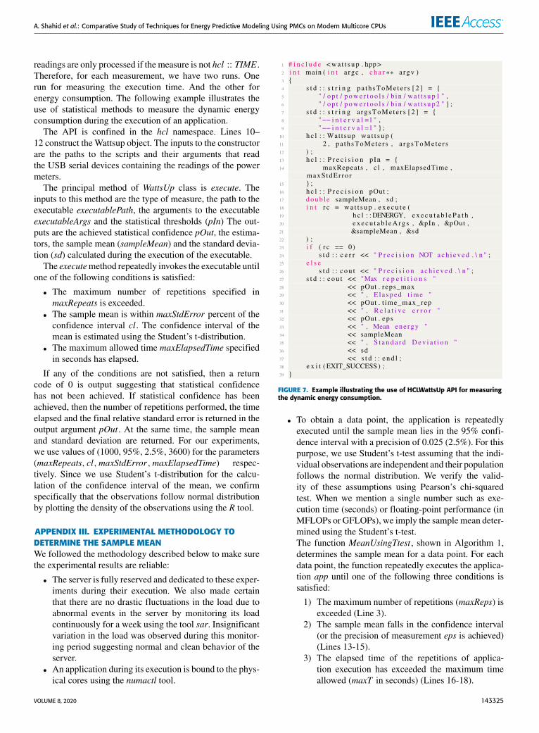
readings are only processed if the measure is not hcl :: TIME .Therefore, for each measurement, we have two runs. Onerun for measuring the execution time. And the other forenergy consumption. The following example illustrates theuse of statistical methods to measure the dynamic energyconsumption during the execution of an application.

The API is confined in the hcl namespace. Lines 10–12 construct the Wattsup object. The inputs to the constructorare the paths to the scripts and their arguments that readthe USB serial devices containing the readings of the powermeters.

The principal method of WattsUp class is execute. Theinputs to this method are the type of measure, the path to theexecutable executablePath, the arguments to the executableexecutableArgs and the statistical thresholds (pIn) The out-puts are the achieved statistical confidence pOut, the estima-tors, the sample mean (sampleMean) and the standard devia-tion (sd) calculated during the execution of the executable.

The executemethod repeatedly invokes the executable untilone of the following conditions is satisfied:

• The maximum number of repetitions specified inmaxRepeats is exceeded.

• The sample mean is within maxStdError percent of theconfidence interval cl. The confidence interval of themean is estimated using the Student’s t-distribution.

• The maximum allowed time maxElapsedTime specifiedin seconds has elapsed.

If any of the conditions are not satisfied, then a returncode of 0 is output suggesting that statistical confidencehas not been achieved. If statistical confidence has beenachieved, then the number of repetitions performed, the timeelapsed and the final relative standard error is returned in theoutput argument pOut . At the same time, the sample meanand standard deviation are returned. For our experiments,we use values of (1000, 95%, 2.5%, 3600) for the parameters(maxRepeats, cl,maxStdError,maxElapsedTime) respec-tively. Since we use Student’s t-distribution for the calcu-lation of the confidence interval of the mean, we confirmspecifically that the observations follow normal distributionby plotting the density of the observations using the R tool.

APPENDIX III. EXPERIMENTAL METHODOLOGY TODETERMINE THE SAMPLE MEANWe followed the methodology described below to make surethe experimental results are reliable:

• The server is fully reserved and dedicated to these exper-iments during their execution. We also made certainthat there are no drastic fluctuations in the load due toabnormal events in the server by monitoring its loadcontinuously for a week using the tool sar. Insignificantvariation in the load was observed during this monitor-ing period suggesting normal and clean behavior of theserver.

• An application during its execution is bound to the phys-ical cores using the numactl tool.

FIGURE 7. Example illustrating the use of HCLWattsUp API for measuringthe dynamic energy consumption.

• To obtain a data point, the application is repeatedlyexecuted until the sample mean lies in the 95% confi-dence interval with a precision of 0.025 (2.5%). For thispurpose, we use Student’s t-test assuming that the indi-vidual observations are independent and their populationfollows the normal distribution. We verify the valid-ity of these assumptions using Pearson’s chi-squaredtest. When we mention a single number such as exe-cution time (seconds) or floating-point performance (inMFLOPs or GFLOPs), we imply the sample mean deter-mined using the Student’s t-test.The function MeanUsingTtest , shown in Algorithm 1,determines the sample mean for a data point. For eachdata point, the function repeatedly executes the applica-tion app until one of the following three conditions issatisfied:

1) The maximum number of repetitions (maxReps) isexceeded (Line 3).

2) The sample mean falls in the confidence interval(or the precision of measurement eps is achieved)(Lines 13-15).

3) The elapsed time of the repetitions of applica-tion execution has exceeded the maximum timeallowed (maxT in seconds) (Lines 16-18).

VOLUME 8, 2020 143325


Algorithm 1 Function Determining the Mean of an Experi-mental Run Using Student’s t-Test1: procedureMeanUsingTtest(app,minReps,maxReps,

maxT , cl, accuracy,repsOut, clOut, etimeOut, epsOut,mean)

Input:The application to execute, appThe minimum number of repetitions, minReps ∈ Z>0The maximum number of repetitions, maxReps ∈ Z>0The maximum time allowed for the application to run,maxT ∈ R>0The required confidence level, cl ∈ R>0The required accuracy, eps ∈ R>0

Output:The number of experimental runs actually made,repsOut ∈ Z>0The confidence level achieved, clOut ∈ R>0The accuracy achieved, epsOut ∈ R>0The elapsed time, etimeOut ∈ R>0The mean, mean ∈ R>0

2: reps← 0; stop← 0; sum← 0; etime← 03: while (reps < maxReps) and (!stop) do4: st ← measure(TIME)5: Execute(app)6: et ← measure(TIME)7: reps← reps+ 18: etime← etime+ et − st9: ObjArray[reps]← et − st

10: sum← sum+ ObjArray[reps]11: if reps > minReps then12: clOut ← fabs(gsl_cdf_tdist_Pinv(cl, reps −

1))× gsl_stats_sd(ObjArray, 1, reps)/ sqrt(reps)

13: if clOut × repssum < eps then

14: stop← 115: end if16: if etime > maxT then17: stop← 118: end if19: end if20: end while21: repsOut ← reps; epsOut ← clOut × reps

sum22: etimeOut ← etime; mean← sum

reps23: end procedure

So, for each data point, the function MeanUsingTtestreturns the sample mean mean. The function Measuremeasures the execution time using gettimeofdayfunction.

• In our experiments, we set the minimum and the max-imum number of repetitions, minReps and maxReps,to 15 and 100000. The values of maxT , cl, and eps are

3600, 0.95, and 0.025. If the precision of measurementis not achieved before the completion of the maximumnumber of repeats, we increase the number of repetitionsand also the allowed maximum elapsed time. Therefore,we make sure that statistical confidence is achieved forall the data points that we use in our experiments.

APPENDIX IV. STEPS TO ENSURERELIABLE EXPERIMENTSTo ensure the reliability of our results, we follow a statisticalmethodology where a sample mean for a response variable isobtained from several experimental runs. The sample meanis calculated by executing the application repeatedly until itlies in the 95% confidence interval and a precision of 0.025(2.5%) has been achieved. For this purpose, Student’s t-testis used assuming that the individual observations are inde-pendent and their population follows the normal distribution.We verify the validity of these assumptions by plotting thedistributions of observations.

The server is fully dedicated for the experiments.To ensure reliable energy measurements, we took followingprecautions:

1) HCLWattsUpAPI [65] gives the total energy consump-tion of the server during the execution of an applicationusing physical measurements from the external powermeters. This includes the contribution from compo-nents such as NIC, SSDs, fans, etc. To ensure that thevalue of dynamic energy consumption is purely dueto CPUs and DRAM, we verify that all the compo-nents other than CPUs and DRAM are idle using thefollowing steps:

• Monitoring the disk consumption before and dur-ing the application run. We ensure that there is noI/O performed by the application using tools suchas sar, iotop, etc.

• Ensuring that the problem size used in the execu-tion of an application does not exceed the mainmemory, and that swapping (paging) does notoccur.

• Ensuring that network is not used by the applica-tion using monitoring tools such as sar, atop, etc.

• Bind an application during its execution toresources using cores-pinning and memory-pinning.

2) Our platform supports three modes to set the fansspeed: minimum, optimal, and full. We set the speedof all the fans to optimal during the execution of ourexperiments. We make sure there is no contribution tothe dynamic energy consumption from fans during anapplication run, by following the steps below:

• We continuously monitor the temperature of serverand the speed of fans, both when the server isidle, and during the application run. We obtain thisinformation by using Intelligent PlatformManage-ment Interface (IPMI) sensors.

143326 VOLUME 8, 2020


• We observed that both the temperature of serverand the speeds of the fans remained the samewhether the given application is running or not.

• We set the fans at full speed before starting theapplication run. The results from this experimentwere the same as when the fans were run at optimalspeed.

• To make sure that pipelining, cache effects, etc,do not happen, the experiments are not executed ina loop and sufficient time (120 seconds) is allowedto elapse between successive runs. This time isbased on observations of the times taken for thememory utilization to revert to base utilization andprocessor (core) frequencies to come back to thebase frequencies.

APPENDIX V. CALIBRATION OF WattsUp PROPOWER-METERSThe dynamic energy consumption during the application exe-cution is measured using a WattsUp Pro power meter onboth servers (HCLServer1 and HCLServer2) and obtainedprogrammatically via the HCLWattsUp interface [65]. Thepower meter is periodically calibrated using an ANSIC12.20 revenue-grade power meter, Yokogawa WT210.In this chapter, we explain our methodology and some resultsto calibrate our power-meters.

We compare theWattsUp Pro power-meter powermeasure-ments with Yokogawa using three methods that are explainedas follows:

1) Naked-eye visual monitoring

• We first attach the WattsUp Pro power-meters toboth servers.

• Once the servers are switched on and are in stablecondition, we monitor the WattsUp pro LCDs andnote the power readings in watts for both servers.

• we carefully plugged off the WattsUp Pro powermeters and plug the servers via Yokogawa powermeter.

• Once the servers are switched on and are in stablecondition, we monitor the Yokogawa LCDs andnote the power readings in watts for both servers.

• On comparison, we find a difference of 2 watts and3 watts for HCLServer1 and HCLServer2, respec-tively.

2) Monitoring server base power

• We connect both power meters to both servers oneby one and once the servers are stable, we program-matically obtain the power readings from bothpower meters.

• For WattsUp Pro, a Perl script provides the powerreadings with a granularity of 1 second. Simi-larly, Yokogawa comes with its own software andallows us to read power readings at the granularityof 1 second.

FIGURE 8. Calibration test for idle power using WattsUp Pro andYokogawa PowerMeter on (a) HCLServer1 and (b) HCLServer2.

• We measure and record the base powers ofboth servers for 3.5 hours using both powermeters. Figure 8 compare the idle power pro-files of HCLServer1 and HCLserver2 using bothpower meters, respectively. It can be seen thatboth profiles are almost the same. However,HCLServer1 has more power variations andHCLServer2 is considerably stable in terms of basepower. For HCLServer2, there are power spikesafter every half an hour for a couple of seconds.This is because of a daemon service being trig-gered by the OS.

• Table 16 show the minimum, average, and max-imum power consumption for both servers andpower meters. If we compare the average,WattsUpPro gives 1-2 watts less power consumption thanYokogawa.

3) Measurement of total energy consumption for twoscientific applications

• We choose two scientific applications: 1) DGEMMand 2) FFT from Intel MKL.

• We execute DGEMM for problem sizes 4096 ×4096 to 30720 × 30720 with a constant stepsize of 1024 on HCLServer1. We then executeDGEMM for problem sizes 15360 × 15360 to30720×30720 with a constant step size of 1024 onHCLServer2. We build the total energy consump-tion profiles using both power meters for theseapplication executions.

• We execute FFT for problem sizes 4096× 4096 to30720×30720 with a constant step size of 1024 onHCLServer1. We then execute FFT for problemsizes 8384 × 8384 to 62880 × 62880 with a con-stant step size of 2096 on HCLServer2. We build

VOLUME 8, 2020 143327


TABLE 16. Minimum, maximum and average of idle power using WattsUp Pro and Yokogawa PowerMeter on HCLServer1 and HCLServer2.

TABLE 17. Comparison of minimum, average, and maximum measurement errors for DGEMM and FFT on HCLServer1 and HCLServer2 using WattsUp Proand Yokogawa.

FIGURE 9. Comparison of total power for Intel MKL DGEMM usingWattsUp Pro and Yokogawa PowerMeter on (a) HCLServer1 and(b) HCLServer2.

the total energy consumption profiles using bothpower meters for these application executions.

• Figure 9 and 10 show the total energy consumptionprofiles for DGEMM and FFT on both servers,respectively.

• Table 17 show the relative error in percent-age for total energy consumptions obtained

FIGURE 10. Comparison of total power for Intel MKL FFT using WattsUpPro and Yokogawa PowerMeter on (a) HCLServer1 and (b) HCLServer2.

using HCLServer1 and HCLServer2. It can beseen that the average measurement error for

143328 VOLUME 8, 2020


DGEMM is 4.95% and 9.25% on HCLServer2 andHCLServer1, respectively. For FFT, the aver-age measurement error is 6% and 7.4% onHCLServer2 and HCLServer1, respectively.

APPENDIX VI. METHODOLOGY TO DETERMINE THECOMPONENT-LEVEL ENERGY CONSUMPTIONUSING HCLWattsUpWe provide here the details of how system-level physicalmeasurements using HCLWattsUp can be used to determinethe energy consumption by a component (such as a CPU)during application execution.

We define the group of components running a givenapplication kernel as an abstract processor. For example,consider a matrix multiplication application running on amulticore CPU. The abstract processor for this application,which we call AbsCPU, comprises of the multicore CPUprocessor consisting of a certain number of physical coresand DRAM. In this work, we use only such configura-tions of the application which execute on AbsCPU anddo not use any other system resources such as solid-statedrives (SSDs), network interface cards (NIC) and so forth.Therefore, the change in energy consumption of the sys-tem reported by HCLWattsUp reflects solely the contribu-tions from CPU and DRAM. We take several precautions incomputing energy measurements to eliminate any potentialinterference of the computing elements that are not part ofthe abstract processor AbsCPU. To achieve this, we take thefollowing precautions:

1) We ensure the platform is reserved exclusively andfully dedicated to our experiments.

2) We monitor the disk consumption before and duringthe application run and ensure that there is no I/Operformed by the application using tools such as sar,iotop, and so forth.

3) We ensure that the problem size used in the executionof an application does not exceed the main memory andthat swapping (paging) does not occur.

4) We ensure that the network is not used by the applica-tion by monitoring using tools such as sar, atop, etc.

5) We set the application kernel’s CPU affinitymask usingSCHED API’s system call SCHED_SETAFFINITY.Consider for example MKL DGEMM application ker-nel running on only abstract processor A. To bind thisapplication kernel, we set its CPU affinity mask to12 physical CPU cores of Socket 1 and 12 physicalCPU cores of Socket 2.

6) Fans are also a great contributor to energy consump-tion. On our platform fans are controlled in two zones:(a) zone 0: CPU or System fans, (b) zone 1: Peripheralzone fans. There are 4 levels to control the speed offans:• Standard: BMC control of both fan zones, withCPU zone based on CPU temp (target speed 50%)and Peripheral zone based on PCH temp (targetspeed 50%)

FIGURE 11. SLOPE-PMC : Towards the automation of PMC collection onModern Computing Platforms.

• Optimal: BMC control of the CPU zone (targetspeed 30%), with Peripheral zone fixed at lowspeed (fixed 30%)

• Heavy IO: BMC control of CPU zone (target speed50%), Peripheral zone fixed at 75%

• Full: all fans running at 100%

In all speed levels except the full, the speed issubject to be changed with temperature and conse-quently, their energy consumption also changes withthe change of their speed. Higher the temperatureof CPU, for example, higher the fans’ speed ofzone 0 and higher the energy consumption to cooldown. This energy consumption to cool the serverdown, therefore, is not consistent and is dependenton the fans’ speed and consequently can affect thedynamic energy consumption of the given applicationkernel.Hence, to rule out the fans’ contribution to dynamicenergy consumption, we set the fans at full speed beforelaunching the experiments. When set at full speed,the fans run consistently at a fixed speed until we do soto another speed level. Hence, fans consume the sameamount of power which is included in the static powerof the platform.

7) We monitor the temperature of the platform and speedof the fans (after setting it at full) with help of Intelli-gent Platform Management Interface (IPMI) sensors,both with and without the application run. We findno considerable difference in temperature and find thespeed of fans the same in both scenarios.

Thus, we ensure that the dynamic energy consumptionobtained using HCLWattsUp reflects the contribution solelyby the abstract processor executing the given applicationkernel.

VOLUME 8, 2020 143329


FIGURE 12. AdditivityChecker : Test PMCs for Additivity.

FIGURE 13. List of PMC groups provided by Likwid tool on HCLServer2.

APPENDIX VII. BRIEF OVERVIEW OF SLOPE-PMC ANDAdditivityCheckerSLOPE-PMC is developed on top of Likwid tool to automatethe process of PMC collection. It takes an input applicationand operates in three steps. First, it identify the availablePMCs on a given platform and list them in a file. In secondstep, the input application is executed several times as ina single invocation of an application only 4 PMCs can be

collected. To ensure reliable results, we also take an averageof each PMC count using multiple executions (atleast 3) ofan application. In the final step, the PMCs are extracted withlabels in a stats file. Figure 11 summarizes the work-flow ofSLOPE-PMC.

Figure 12 describes the AdditivityChecker where it takesas an input: 1). PMCs of two base applications A and B,and a compound application (AB) composed of base applica-tions and 2). user-specified tolerance in percentage. It returnsa list of additive and non-additive PMCs along with theirpercentage errors.

APPENDIX VIII. LIST OF PMC GROUPSPROVIDED BY LIKWIDThe list of PMC groups provided by Likwid tool [16] onHCLServer2 is shown in the Figure 13.

REFERENCES[1] N. Jones, ‘‘How to stop data centres from gobbling up the world’s electric-

ity,’’ Nature, vol. 561, no. 7722, pp. 163–166, 2018.[2] A. Andrae and T. Edler, ‘‘On global electricity usage of communication

technology: Trends to 2030,’’ Challenges, vol. 6, no. 1, pp. 117–157,Apr. 2015.

[3] J. Yang, X. Zhou, M. Chrobak, Y. Zhang, and L. Jin, ‘‘Dynamic thermalmanagement through task scheduling,’’ in Proc. IEEE Int. Symp. Perform.Anal. Syst. Softw. (ISPASS), Apr. 2008, pp. 191–201.

[4] R. Z. Ayoub and T. S. Rosing, ‘‘Predict and act: Dynamic thermal man-agement for multi-core processors,’’ in Proc. ACM/IEEE Int. Symp. LowPower Electron. Design, Aug. 2009, pp. 99–104.

[5] W. Wang, P. Mishra, and S. Ranka, ‘‘Dynamic cache reconfiguration andpartitioning for energy optimization in real-time multi-core systems,’’ inProc. 48th Design Autom. Conf. (DAC), Jun. 2011, pp. 948–953.

[6] S. Zhuravlev, J. C. Saez, S. Blagodurov, A. Fedorova, and M. Prieto, ‘‘Sur-vey of scheduling techniques for addressing shared resources in multicoreprocessors,’’ ACM Comput. Surv., vol. 45, no. 1, pp. 1–28, Nov. 2012.

[7] G. Chen, K. Huang, J. Huang, and A. Knoll, ‘‘Cache partitioning andscheduling for energy optimization of real-time MPSoCs,’’ in Proc.IEEE 24th Int. Conf. Appl.-Specific Syst., Archit. Processors, Jun. 2013,pp. 35–41.

[8] V. Petrucci, O. Loques, D. Mossé, R. Melhem, N. A. Gazala, andS. Gobriel, ‘‘Energy-efficient thread assignment optimization for heteroge-neous multicore systems,’’ ACM Trans. Embedded Comput. Syst., vol. 14,no. 1, pp. 1–26, Jan. 2015.

[9] Y. G. Kim, M. Kim, and S. W. Chung, ‘‘Enhancing energy efficiency ofmultimedia applications in heterogeneous mobile multi-core processors,’’IEEE Trans. Comput., vol. 66, no. 11, pp. 1878–1889, Nov. 2017.

[10] J. Demmel, A. Gearhart, B. Lipshitz, and O. Schwartz, ‘‘Perfect strongscaling using no additional energy,’’ in Proc. IEEE 27th Int. Symp. ParallelDistrib. Process., May 2013, pp. 649–660.

[11] J. Lang and G. Rünger, ‘‘An execution time and energy model for anenergy-aware execution of a conjugate gradient method with CPU/GPUcollaboration,’’ J. Parallel Distrib. Comput., vol. 74, no. 9, pp. 2884–2897,Sep. 2014.

[12] A. Chakrabarti, S. Parthasarathy, and C. Stewart, ‘‘A Pareto framework fordata analytics on heterogeneous systems: Implications for green energyusage and performance,’’ in Proc. 46th Int. Conf. Parallel Process. (ICPP),Aug. 2017, pp. 533–542.

[13] A. Lastovetsky and R. Reddy Manumachu, ‘‘New model-based methodsand algorithms for performance and energy optimization of data parallelapplications on homogeneous multicore clusters,’’ IEEE Trans. ParallelDistrib. Syst., vol. 28, no. 4, pp. 1119–1133, Apr. 2017.

[14] R. R. Manumachu and A. Lastovetsky, ‘‘Bi-objective optimization of data-parallel applications on homogeneous multicore clusters for performanceand energy,’’ IEEE Trans. Comput., vol. 67, no. 2, pp. 160–177, Feb. 2018.

[15] M. Fahad, A. Shahid, R. R. Manumachu, and A. Lastovetsky,‘‘A comparative study of methods for measurement of energy ofcomputing,’’ Energies, vol. 12, no. 11, p. 2204, Jun. 2019. [Online].Available: https://www.mdpi.com/1996-1073/12/11/2204

143330 VOLUME 8, 2020


[16] J. Treibig, G. Hager, and G. Wellein, ‘‘LIKWID: A lightweightperformance-oriented tool suite for x86 multicore environments,’’ in Proc.39th Int. Conf. Parallel Process. Workshops, Sep. 2010, pp. 207–216.

[17] J. Mair, Z. Huang, and D. Eyers, ‘‘Manila: Using a densely populatedPMC-space for power modelling within large-scale systems,’’ ParallelComput., vol. 82, pp. 37–56, Feb. 2019.

[18] Z. Zhou, J. H. Abawajy, F. Li, Z. Hu, M. U. Chowdhury, A. Alelaiwi, andK. Li, ‘‘Fine-grained energy consumption model of servers basedon task characteristics in cloud data center,’’ IEEE Access, vol. 6,pp. 27080–27090, 2018.

[19] J. Haj-Yihia, A. Yasin, Y. B. Asher, and A. Mendelson, ‘‘Fine-grain powerbreakdown of modern out-of-order cores and its implications on skylake-based systems,’’ ACM Trans. Archit. Code Optim., vol. 13, no. 4, p. 56,2016.

[20] A. Shahid, M. Fahad, R. Reddy, and A. Lastovetsky, ‘‘Additivity: A selec-tion criterion for performance events for reliable energy predictive model-ing,’’ Supercomput. Frontiers Innov., vol. 4, no. 4, pp. 50–65, Dec. 2017.

[21] A. Shahid, M. Fahad, R. Reddy Manumachu, and A. Lastovetsky,‘‘Energy of computing on multicore CPUs: Predictive models andenergy conservation law,’’ 2019, arXiv:1907.02805. [Online]. Available:http://arxiv.org/abs/1907.02805

[22] PAPI. (2015). Performance Application Programming Interface 5.4.1.[Online]. Available: http://icl.cs.utk.edu/papi/

[23] J.-A. Rico-Gallego, J.-C. Díaz-Martín, and A. L. Lastovetsky, ‘‘Extendingτ -Lop to model concurrent MPI communications in multicore clusters,’’Future Gener. Comput. Syst., vol. 61, pp. 66–82, Aug. 2016. [Online].Available: https://doi.org/10.1016/j.future.2016.02.021

[24] H. Abdi and L. J. Williams, ‘‘Principal component analysis,’’ Wiley Inter-discipl. Rev., Comput. Statist., vol. 2, no. 4, pp. 433–459, 2010.

[25] M. Fahad, A. Shahid, R. R. Manumachu, and A. Lastovetsky, ‘‘Accurateenergy modelling of hybrid parallel applications on modern heterogeneouscomputing platforms using system-level measurements,’’ IEEE Access,vol. 8, pp. 93793–93829, 2020.

[26] E. Rotem, A. Naveh, A. Ananthakrishnan, E. Weissmann, and D. Rajwan,‘‘Power-management architecture of the intel microarchitecture code-named sandy bridge,’’ IEEE Micro, vol. 32, no. 2, pp. 20–27, Mar. 2012.

[27] Nvidia. (Oct. 2018). Nvidia Management Library: NVML ReferenceManual. [Online]. Available: https://docs.nvidia.com/pdf/NVML_API_Reference_Guide.pdf

[28] I. Corporation, ‘‘Intel xeon phi coprocessor system software developersguide,’’ Tech. Rep., Jun. 2014.

[29] M. Burtscher, I. Zecena, and Z. Zong, ‘‘Measuring GPU power with theK20 built-in sensor,’’ in Proc. Workshop Gen. Purpose Process. UsingGPUs, Mar. 2014, p. 28.

[30] P. Wiki. (2017). perf: Linux Profiling With Performance Counters.[Online]. Available: https://perf.wiki.kernel.org/index.php/Main_Page

[31] IntelPCM. 2012. Intel Performance Counter Monitor—ABetter Way to Measure CPU Utilization. [Online]. Available:https://software.intel.com/en-us/articles/intel-performance-counter-monitor

[32] CUPTI. (2017). CUDA Profiling Tools Interface. [Online]. Available:https://developer.nvidia.com/cuda-profiling-tools-interface

[33] L. Benini, A. Bogliolo, S. Cavallucci, and B. Riccó, ‘‘Monitoring systemactivity for OS-directed dynamic power management,’’ in Proc. Int. Symp.Low Power Electron. Design (ISLPED), 1998, pp. 185–190.

[34] Y.-H. Lu, L. Benini, and G. DeMicheli, ‘‘Operating-system directed powerreduction,’’ in Proc. ISLPED00: Proc. Int. Symp. Low Power Electron.Design, Jul. 2000, pp. 37–42.

[35] L. Benini, A. Bogliolo, and G. DeMicheli, ‘‘A survey of design techniquesfor system-level dynamic power management,’’ IEEE Trans. Very LargeScale Integr. (VLSI) Syst., vol. 8, no. 3, pp. 299–316, Jun. 2000.

[36] F. Bellosa, ‘‘The benefits of event: Driven energy accounting in power-sensitive systems,’’ in Proc. 9th Workshop ACM SIGOPS Eur. Workshop:Beyond PC: New Challenges Operating Syst., 2000, pp. 37–42.

[37] C. Isci and M. Martonosi, ‘‘Runtime power monitoring in high-end pro-cessors: Methodology and empirical data,’’ in Proc. 22nd Digit. AvionicsSyst. Conf., Dec. 2003, p. 93.

[38] T. Li and L. K. John, ‘‘Run-time modeling and estimation of operatingsystem power consumption,’’ ACM SIGMETRICS Perform. Eval. Rev.,vol. 31, no. 1, pp. 160–171, Jun. 2003, doi: 10.1145/885651.781048.

[39] B. C. Lee and D. M. Brooks, ‘‘Accurate and efficient regression mod-eling for microarchitectural performance and power prediction,’’ ACMSIGPLAN Notices, vol. 41, no. 11, pp. 185–194, Nov. 2006.

[40] T. Heath, B. Diniz, E. V. Carrera,W.M. Jr., and R. Bianchini, ‘‘Energy con-servation in heterogeneous server clusters,’’ in Proc. 10th ACM SIGPLANSymp. Princ. Pract. Parallel Program. (PPoPP), 2005, pp. 186–195.

[41] D. Economou, S. Rivoire, C. Kozyrakis, and P. Ranganathan, ‘‘Full-systempower analysis and modeling for server environments,’’ in Proc. WorkshopModel., Benchmarking, Simulation, 2006, pp. 70–77.

[42] X. Fan, W.-D. Weber, and L. A. Barroso, ‘‘Power provisioning for awarehouse-sized computer,’’ in Proc. 34th Annu. Int. Symp. Comput.Archit. (ISCA), 2007, pp. 13–23.

[43] A. Kansal and F. Zhao, ‘‘Fine-grained energy profiling for power-awareapplication design,’’ ACM SIGMETRICS Perform. Eval. Rev., vol. 36,no. 2, p. 26, Aug. 2008.

[44] S. Rivoire, P. Ranganathan, and C. Kozyrakis, ‘‘A comparison of high-levelfull-system power models,’’ in Proc. Conf. Power Aware Comput. Syst.,2008, pp. 32–39.

[45] S. Rivoire, ‘‘Models and metrics for energy-efficient computer systems,’’Ph.D. dissertation, Dept. Elect. Eng., Stanford Univ., Stanford, CA, USA,2008.

[46] K. Singh, M. Bhadauria, and S. A. McKee, ‘‘Real time power estimationand thread scheduling via performance counters,’’ ACM SIGARCH Com-put. Archit. News, vol. 37, no. 2, pp. 46–55, May 2009.

[47] M. D. Powell, A. Biswas, J. S. Emer, S. S. Mukherjee, B. R. Sheikh, andS. Yardi, ‘‘CAMP: A technique to estimate per-structure power at run-time using a few simple parameters,’’ in Proc. IEEE 15th Int. Symp. HighPerform. Comput. Archit., Feb. 2009, pp. 289–300.

[48] B. Goel, S. A. McKee, R. Gioiosa, K. Singh, M. Bhadauria, and M. Cesati,‘‘Portable, scalable, per-core power estimation for intelligent resourcemanagement,’’ in Proc. Int. Conf. Green Comput. Chicago, IL, USA: IEEEPress, 2010, pp. 135–146.

[49] H. Wang, Q. Jing, R. Chen, B. He, Z. Qian, and L. Zhou, ‘‘Distributedsystemsmeet economics: Pricing in the cloud,’’ inProc. 2ndUSENIXConf.Hot Topics Cloud Comput., 2010, pp. 1–7.

[50] R. Basmadjian, N. Ali, F. Niedermeier, H. de Meer, and G. Giuliani, ‘‘Amethodology to predict the power consumption of servers in data centres,’’in Proc. 2nd Int. Conf. Energy-Efficient Comput. Netw. (e-Energy), 2011.

[51] W. Dargie, ‘‘A stochastic model for estimating the power consumptionof a processor,’’ IEEE Trans. Comput., vol. 64, no. 5, pp. 1311–1322,May 2015.

[52] S. Hong and H. Kim, ‘‘An integrated GPU power and performance model,’’ACM SIGARCH Comput. Archit. News, vol. 38, no. 3, pp. 280–289,Jun. 2010.

[53] H. Nagasaka, N. Maruyama, A. Nukada, T. Endo, and S. Matsuoka,‘‘Statistical power modeling of GPU kernels using performance counters,’’in Proc. Int. Conf. Green Comput., Aug. 2010, pp. 115–122.

[54] S. Song, C. Su, B. Rountree, and K. W. Cameron, ‘‘A simplified and accu-rate model of power-performance efficiency on emergent GPU architec-tures,’’ in Proc. IEEE 27th Int. Symp. Parallel Distrib. Process., May 2013,pp. 673–686.

[55] Y. S. Shao and D. Brooks, ‘‘Energy characterization and instruction-levelenergymodel of Intel’s xeon phi processor,’’ in Proc. Int. Symp. Low PowerElectron. Design (ISLPED), Sep. 2013, pp. 389–394.

[56] Z. Al-Khatib and S. Abdi, ‘‘Operand-value-based modeling of dynamicenergy consumption of soft processors in FPGA,’’ in Proc. Int. Symp. Appl.Reconfigurable Comput. Darmstadt, Germany: Springer, 2015, pp. 65–76.

[57] M. Witkowski, A. Oleksiak, T. Piontek, and J. Weglarz, ‘‘Practical powerconsumption estimation for real life HPC applications,’’ Future Gener.Comput. Syst., vol. 29, no. 1, pp. 208–217, Jan. 2013.

[58] M. Jarus, A. Oleksiak, T. Piontek, and J. Weglarz, ‘‘Runtime power usageestimation of HPC servers for various classes of real-life applications,’’Future Gener. Comput. Syst., vol. 36, pp. 299–310, Jul. 2014.

[59] X. Wu, V. Taylor, J. Cook, and P. J. Mucci, ‘‘Using performance-powermodeling to improve energy efficiency of HPC applications,’’ Computer,vol. 49, no. 10, pp. 20–29, Oct. 2016.

[60] P. Gschwandtner, M. Knobloch, B. Mohr, D. Pleiter, and T. Fahringer,‘‘Modeling CPU energy consumption of HPC applications on the IBMPOWER7,’’ in Proc. 22nd Euromicro Int. Conf. Parallel, Distrib., Netw.-Based Process., Feb. 2014, pp. 536–543.

[61] J. C. McCullough, Y. Agarwal, J. Chandrashekar, S. Kuppuswamy,A. C. Snoeren, and R. K. and Gupta, ‘‘Evaluating the effectivenessof model-based power characterization,’’ in Proc. 2011 USENIX Conf.USENIX Annu. Tech. Conf., 2011, pp. 1–14.

VOLUME 8, 2020 143331

http://dx.doi.org/10.1145/885651.781048


[62] D. Hackenberg, T. Ilsche, R. Schone, D. Molka, M. Schmidt, andW. E. Nagel, ‘‘Power measurement techniques on standard compute nodes:A quantitative comparison,’’ in Proc. IEEE Int. Symp. Perform. Anal. Syst.Softw. (ISPASS), Apr. 2013, pp. 194–204.

[63] K. O’brien, I. Pietri, R. Reddy, A. Lastovetsky, and R. Sakellariou,‘‘A survey of power and energy predictive models in HPC systems andapplications,’’ ACM Comput. Surveys, vol. 50, no. 3, pp. 1–38, Oct. 2017.

[64] A. Shahid, M. Fahad, R. R. Manumachu, and A. Lastovetsky, ‘‘Improvingthe accuracy of energy predictivemodels for multicore CPUs using additiv-ity of performance monitoring counters,’’ in Parallel Computing Technolo-gies, V. Malyshkin, Ed. Cham, Switzerland: Springer, 2019, pp. 51–66.

[65] H. C. Laboratory and U. C. Dublin. (2020). HCLWattsUp: API for powerand energy measurements using WattsUp Pro Meter. [Online]. Available:https://csgitlab.ucd.ie/ucd-hcl/hclwattsup

[66] A. Liaw and M. Wiener, ‘‘Classification and regression by randomforest,’’R News, vol. 2, no. 3, pp. 18–22, 2002.

[67] F. Dan Foresee and M. T. Hagan, ‘‘Gauss-Newton approximation toBayesian learning,’’ in Proc. Int. Conf. Neural Netw. (ICNN), vol. 3, 1997,pp. 1930–1935.

[68] J. J. Moré, ‘‘The Levenberg–Marquardt algorithm: Implementation andtheory,’’ in Proc. Conf. Numer. Anal., Dundee, U.K. New York, NY, USA:Springer, 1978, pp. 105–116.

ARSALAN SHAHID received the B.S. degreein electrical engineering from HITEC University,Pakistan, in 2016, and the Ph.D. degree fromUniversity College Dublin, in 2020. His researchinterests include energy-aware high-performanceheterogeneous computing and intelligent cloudcomputing.

MUHAMMAD FAHAD received the B.S. degreefrom International Islamic University, Islamabad,Pakistan, in 2008, and the M.S. degree fromthe KTH Royal Institute of Technology, Swe-den, in 2012. He is currently a Ph.D. Researcherwith the Heterogeneous Computing Laboratory(HCL), University College Dublin, Ireland. Hismain research interests include high-performanceheterogeneous computing, energy-efficient com-puting, and parallel/distributed and peer-to-peercomputing.

RAVI REDDY MANUMACHU received theB.Tech. degree from IIT Madras, in 1997, andthe Ph.D. degree from the School of ComputerScience, University College Dublin, in 2005. Hismain research interests include high-performanceheterogeneous computing, distributed computing,energy-efficient computing, and sparse matrixcomputations.

ALEXEY LASTOVETSKY received the Ph.D.degree from the Moscow Aviation Institute,in 1986, and the Doctor of Science degree fromthe Russian Academy of Sciences, in 1997.He has published over a 100 technical papersin refereed journals, edited books, and interna-tional conferences. He has authored the mono-graphs Parallel Computing on Heterogeneous Net-works (Wiley, 2003) and High-Performance Het-erogeneous Computing (Wiley, 2009). His main

research interests include algorithms, models, and programming tools forhigh-performance heterogeneous computing.

143332 VOLUME 8, 2020

Documents

A Comparative Study of Techniques for Energy ... - hcl.ucd.ie