A COMPARATIVE ANALYSIS OF RECENT EXPORT PERFORMANCES OF CHINA AND INDIA*

Kaliappa Kalirajan Foundation for Advanced Studies on International Development and

National Graduate Institute for Policy Studies 7-22-1 Roppongi

Minato-ku Tokyo 106-8677

Japan and

Kanhaiya Singh National Council of Applied Economic Research

Parisila Bhawan 11, Indraprastha Estate

New Delhi 110 002 India

* Paper presented at the Asian Economic Panel Meeting at the Brookings Institution, Washington, D.C. on 10 April 2007. Comments and suggestions on an earlier version by discussants, Lael Brainard, Brookings Institution, and Zhang Xiaojing, Chinese Academy of Social Sciences, and participants are gratefully acknowledged. A special thanks to Wing Thye Woo for commissioning this study for this Panel Meeting.

2

A COMPARATIVE ANALYSIS OF RECENT EXPORT PERFORMANCES OF CHINA AND INDIA

Abstract

Drawing on the convergence theory, one would expect that as a

latecomer to integrate with the globalised economy India’s export

performance would be at least on par with that of China because

China’s performance has been as predicted by the theory. This study,

using performance measures based on the endogenous growth theory

that internalises the ability to export the maximum possible exports

under the determinants of exports including the existing ‘behind the

border’ and ‘beyond the border’ constraints, shows that India’s export

performance is still far behind that of China. The implication of this

study is that India’s reform measures need to be intensified

effectively to catch up and to overtake China.

JEL Classifications: C24, F10, and F14,

Key words: Export performance, ‘behind the border constraints,

‘beyond the border constraints’, potential exports, China, India.

3

1. Introduction In the ranking of the largest economies of the world measured by their gross domestic

products in terms of 1995 constant US$, China and India stood at the 19th and 20th

positions in 1980, but in 2005 the ranking places them at the 7th and 12th positions

respectively. Such a quantum jump of these two economies, particularly China, over two

and a half decades is remarkable1. What is interesting to know is, measured in terms of

per capita income in current international dollars with purchasing power parity, China

was lagging behind India by $ 223 in 1980, but overtook India with a difference of

$ 1,450 in 2000. Based on the IMF data, the per capita income in current international

dollars with purchasing power parity in 2005 worked out to be $ 3,320 and $ 7,150 for

India and China respectively. Such a dynamic growth performance of China and a

respectable growth performance of India raise several interesting questions2.

For example, is China’s growth miracle different from what we observed in other Asian

countries? While China has demonstrated its potential to grow faster consistently for

several years, why doesn’t India exhibit the same kind of dynamism? As a latecomer,

what can India learn from China’s growth process? These interesting and important

questions have occupied the minds of development economists always. There is now rich

literature on the economic developments of these two countries including their reform

processes and their impacts on macroeconomic policies and overall economic growth.

Though some of the conclusions in these studies are controversial, there is consensus that

1 Sachs and Woo (2000) have provided a comprehensive exposition about the factors behind the successful economic performance of China. 2 In the eyes of many observers, by the end of the 1990s India had moved to being a “six percent growth” economy: not a ‘miracle’ perhaps, but certainly respectable.

4

opening up the economies for export-led-growth through trade liberalization is a crucial

factor among others, which significantly influenced the growth performance3.

Is China’s growth performance anything special? When China’s growth experience is

examined against the growth patterns of other Asian countries, particularly Japan, it is

noticeable that Japan’s growth rate fell 15 years after its catching-up process started in

1955, whereas China has continued its growth for more than 25 years4. However, when

China’s share of global GDP is compared with that of Japan’s, it is evident that the

latter’s share of global GDP grew faster than that of the former during Japan’s catching-

up process. Thus, there does not seem to be any significant miracles in the growth

performances of China when compared it with that of Japan5. Nevertheless, China’s

growth performance looks more impressive, if its integration into the global economy in

terms of international trade in goods is considered.

For example, China’s total merchandise trade increased from $1,155 billion in 2004 to

$1,422 billion during 2005. The surge in China’s exports has drastically changed the

structure of East Asia’s trade surplus with the U.S. and the European Union in favour of

China from Japan. Drawing on the ‘convergence theory’, if, as a latecomer, China has

been able to improve its export performance faster, why not India, which opened up its

economy much later than China? It is in this context, this paper examines merchandise

3 For example, some authors have found differences in the political system as the key instrument creating differences in the performance of the two countries. Sachs and Woo (2000) labeled the competing interpretations of China's post-1978 economic growth process as institutional innovations versus institutional convergence, which are in other words, the Experimentalist School and the Convergence School respectively. Important econometric studies of the linkage between trade reform and the rate of economic growth include Sachs and Warner (1995), and Frankel and Romer (1999). 4 The starting period of the catching-up process for a country is based on the IMF’s notion of having an annual rise in exports of more than 10% for three years continuously (IMF, World Economic Outlook, Chapter II, 2004). 5 In this context, it is worth noting the publication by Garnaut and Huang (2001), which is titled as ‘Growth without Miracles’.

5

export performances of China and India with the following three empirical questions: (a)

If China’s exporting environment is emulated by India, what would be the latter’s export

performance? (c) If India’s exporting environment is duplicated by China, what would be

the latter’s export performance? and (c) How far have been China and India from

reaching their exports potential with their trading partners given the existing ‘behind the

border constraints’ and ‘beyond the border constraints’ to exports?6

The following section briefly describes important trade policy reforms of China and

India. The next section discusses the concept and measurements of potential exports and

data, which is followed by empirical estimations of different measures of potential

exports of China and India with their trading partners. This section also provides the

simulation results of export performances of China and India with the assumption of

China emulating the exporting environment of India and India duplicating the exporting

environment of China respectively. A final section discusses what India can learn from

the export performance of China to shape up its trade policy reforms.

2. Trade Policy Reforms of China and India

2.1. China

Trade policy in China underwent a major change during 1979-1980, when the central

government decided to establish four Special Economic Zones (SEZs) in two coastal

provinces, Guangdong and Fujian, to attract foreign direct investment and new

technologies. This was the beginning of the Open-Door Policy of China. Initial success

6 “Behind the border constraints” to export, within the home country, which mainly include regulatory policies that impede competition, restrictions on foreign trade and investment, tolerance of business cartels, monopoly privileges given to public enterprises, and the cost and performance of infrastructure services that are important to the functioning of businesses, services such as ports, customs and transport, generally affect the domestic costs of production. “Beyond the border constraints” mainly refer to non-tariff barriers and other institutional rigidities of partner countries, which generally influence the shifting of the export frontier.

6

encouraged Chinese policymakers to adopt similar policies in 14 east coastal cities in

1984, which were further extended to a far wider area of China’s east coast region in

1985 and in the following years. It is worth noting that the 12 East Coast provinces, out

of the total 30,7 contributed 2/3 of China’s total exports in 1990. The openness of the

Chinese economy was accelerated in the 1990s, after Deng Xiaoping’s push for

acceleration of economic reform and openness in 1992. Twenty inland cities became

“open cities” that could enjoy a series of preferential policies in 1993. Border areas in the

North and West China, i.e., Xinjiang, Inner Mongolia, Heilongjiang, Yuannan and

Guangxi, were also opened to border trade (Wang, 2004).

FDI increased dramatically in the 1990s, which was only US$ 1.7 billion in 1985. In

1995, FDI increased to 37.5 billion, and then to 40.7 billion in 2000, and to 72.4 billion in

2005. Domestic and foreign trade sectors were opened to FDI in the late 1990s. Foreign

enterprises, which include enterprises with investment from Chinese Hong Kong, Macao

and Taiwan, played more and more important roles in the manufacturing sector of China

(Jiang, 2002).

Trade policy was not immediately shifted from import-substitution to export-orientation.

During a long period of the reform era, it was a mix of both import-substitution and

export-orientation, but gradually shifted towards the East Asian growth model of export-

oriented growth. China remained with high import tariffs, although the real tariff rate was

far lower, due to various preferential policies and smuggling. In 1995, for example, the

average nominal tariff rate on electronic products was 40 percent, but the actual rate (that

7 This includes four Minority Autonomous Regions and three Central-Administrated Municipalities. The total number became 31 later.

7

is, tariffs actually collected as a share of the value of imports) was only 11.8 percent

(Wang, 2004).

There were also trade-related investment measures (TRIMs) in the 1980s and 1990s, such

as domestic component, export performance, and foreign exchange balance requirements,

to ensure the national trade balance. In spite of these, the foreign-invested industries were

not a foreign-exchange earner in the 1980s and early-to-middle 1990s, because their

exports could not exceed their imports before 1998, though it did contribute to economic

growth, employment generation and increase in foreign trade to a large extent (Wang,

2004).

There were more changes in the 1990s. In 1996, joint ventures with foreign investment

were allowed to deal with foreign trade. In 1998, private enterprises were also allowed to

engage in foreign trade. The state monopoly in foreign trade was gradually replaced by

market competition. Deduction, or removal, of tariff and non-tariff barriers was also an

important part of trade policy reform. During the 1982-1992 period, the nominal tariff

rate, as an average, reduced from 56% to 43%. During the 1992-2003 period, it further

reduced from 43% to 11% (Wu, 2003).8 The average tariff in 2005 was 9.9%. Non-tariff

barriers, e.g., import licensing and requirement for special import approvals, were

reduced in the 1990s and basically eliminated in the early 2000s, as the government’s

commitment upon the WTO accession.

There were major changes after the WTO accession in 2001 too. Concerning TRIMs,

mainly requirements on domestic component, export performance and foreign exchange

8 As mentioned earlier, the actual tariff rate in the 1990s should be far below the officially announced rate because of various tariff exemptions and deductions, and smuggling. This should not be the case in the early 1980s, because the coverage of policy preferences on tariff deduction was only limited at the time, and smuggling was less serious.

8

balance of foreign enterprises, were removed. Upon China’s WTO accession in 2001, the

banking and insurance, and telecommunication sectors, which were not opened to FDI

before, were opened.9 Not only the trade policies relating to FDI were changed, trade

liberalization also occurred in the domestic sectors. More and more manufacturers that

producing export goods were also permitted to directly purchase inputs and sell products

overseas. Thus, it is apparent that trade policy reforms significantly contributed to

economic growth in China, which was more or less on average at the two-digit level over

more than two decades.10

Nevertheless, there are rooms for further improvement in China’s trade policies11. Some

analysts have suggested that the imbalance of policy treatment between FDI and domestic

investment, which favours FDI, has resulted in rent-seeking behaviour and inefficiencies.

In addition, there are needs for further policy reform towards transparency and better

business environment (Huang and Khanna, 2003; Sachs and Woo, 2002).

2.2. India

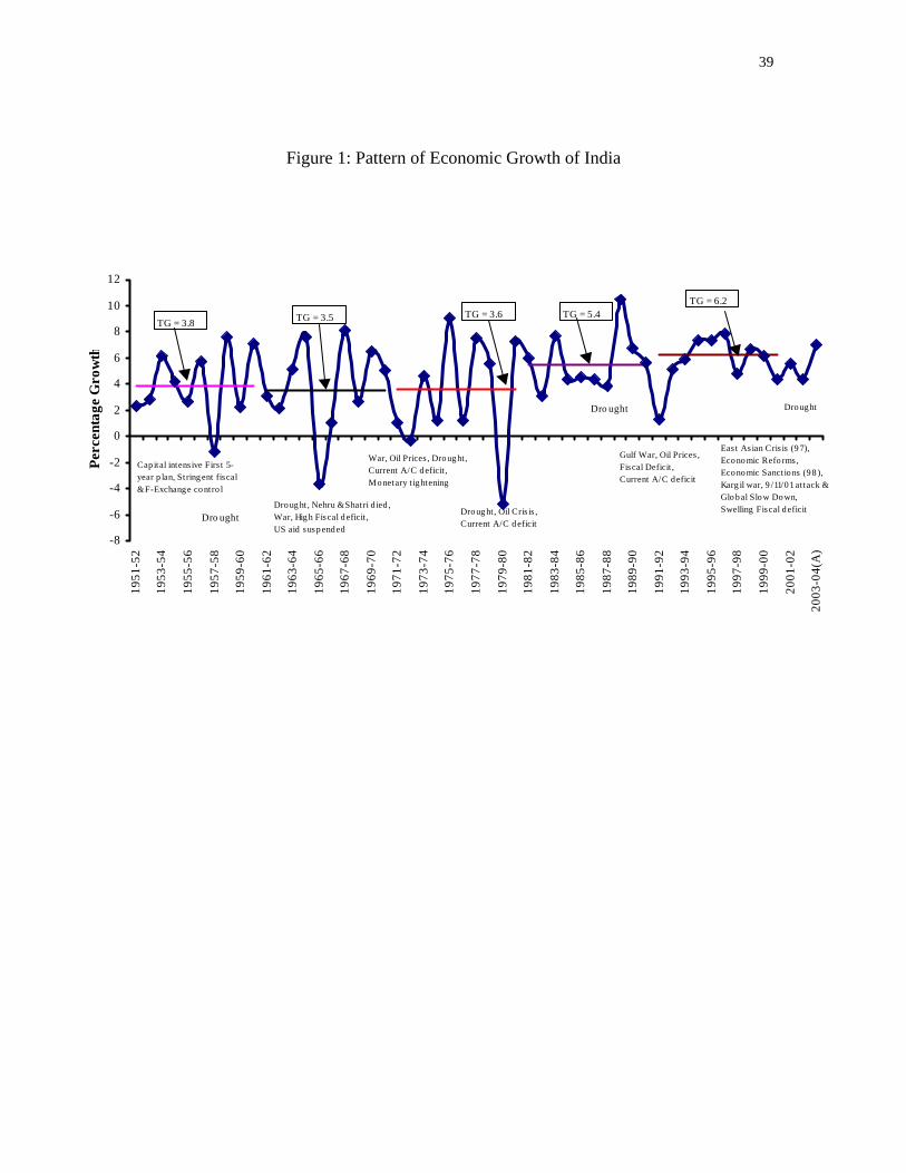
Figure 1 presents a simplified record of India’s aggregate growth (growth in real GDP at

factor cost, 1993-94 prices) performance over the 52 years from 1951-52 to 2002-03. It

also plots trend growth (TG) rates for each decade starting 1951-61 and some of the key

events responsible for slowdown episodes and a summary table indicating the coefficient

of variation across decades and average growths after ignoring the drought and crisis

9 Sachs and Woo (2002) have argued that the Chinese leadership’s opinion has been that in the short-run, there could be significant displacement of Chinese state banks by foreign banks, but in the long run, Chinese banks (most likely private ones) would rise in importance. 10 Literature indicates that countries, which liberalized their trade (raising their trade-to-GDP ratio by an average of 5percentage points) between 1950 and 1998 enjoyed on average 1.5 percentage points higher GDP growth compared with their pre-reform growth rates (Greenaway, et al., 2002; and Baldwin, 2003). 11 Drysdale, Huang, and Kalirajan (2000) have argued for the need for more trade policy reforms to enhance China’s trade efficiency. Gang Fan and Xiaojing Zhang (2003) have discussed how the further reform agenda can be designed to achieve another period of two decades of high growth.

9

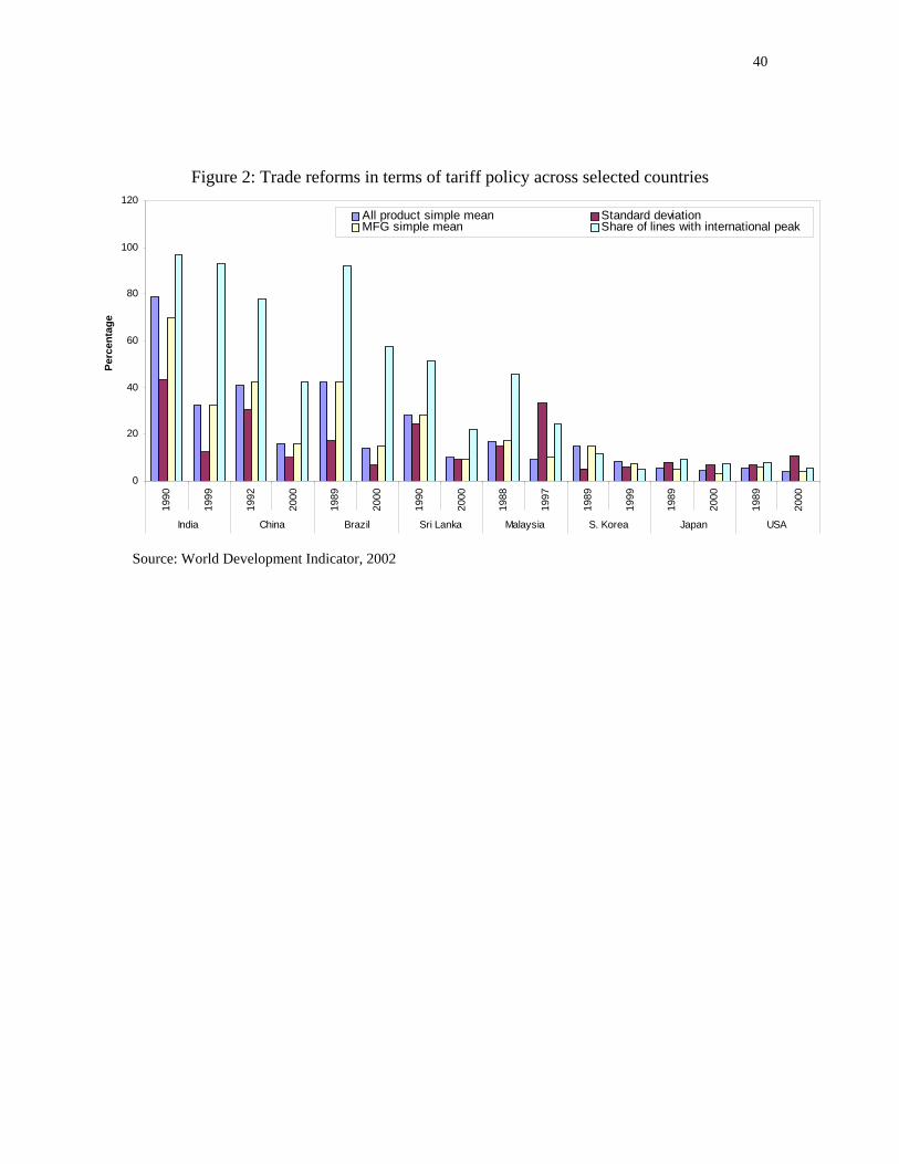
periods. Sweeping policy changes were made in the trade sector during the 1990s in

India, though at a pace slower than in China. Customs tariffs are now lower and

quantitative restrictions on imports have been done away with. Export restrictions have

been reduced along with the implementation of various export promotion measures.

However, the pace of tariff reforms slowed down after 1996-97. While the peak rate of

duty has been reduced gradually, the average tariff rate remained broadly unchanged at

about 30 per cent during 1997-2002, though the average tariff was about 18% in 2005,

which is almost double that of China. This tariff rate is also very high by the current

world standards. Figure 2 shows plots of four indicators of tariff-related trade barriers,

all-products simple mean, standard deviation of tariff lines, simple mean of tariff lines for

manufactured goods, and share of tariff lines with international peaks. When compared

with countries, such as China, Brazil, South Korea, Sri Lanka, Malaysia, Japan and the

United States, India turns out to be an outlier in terms of all-products simple mean tariffs.

What is most disturbing is the number of lines with world peak. It appears that the Indian

authorities simply look at the highest rates prevailing anywhere in the world and adopt

the same as tariff without much analysis.

There are also concerns about the institutional role in determining tariff. At least four

institutions are assigned the role of fixing tariffs in one way or the other. Among them the

most relevant department, the Tariff Commission, which has resources to determine

tariffs with more techno-economic analysis has never been involved in tariff

determination or regulation since its inception in September 1997. Then, there is a tariff

research unit (TRU) in the revenue department of the Ministry of Finance, presumably

most effective in determining tariff, which obviously would be more concerned about

10

short-term effects of changes in tariffs, particularly on revenue than long-term effects on

trade and growth. The Ministry of Agriculture reportedly determines agricultural tariffs.

Besides, there is an anti-dumping directorate in the ministry of commerce to look into

complaints of dumping. Thus, lack of institutional co-ordination may not be overlooked.

Though the medium-term exports strategy (MTES 2002-2007), which was announced in

January 2002, aimed to increasing India’s share in world trade from about 0.7 per cent to

1 per cent by 2006-07, the current target is to reach 1.5% of world trade by 2009.12 Latest

trade figures in the World Trade Report 2006 reveal that in calendar year 2005, India’s

merchandise exports were worth $90billion that is approximately 0.89% of total global

exports worth $10,121billion. China’s share, on the other hand, increased from 6.67% in

2004 to 7.52% in 2005 with the country exporting goods worth $762billion during the

year. While India’s share in world total merchandise exports surged from 0.4% in 1992 to

0.8% in 2002, it took three long years for India to move another step further. At this rate,

the target of reaching 1.5% of world trade by 2009 would not be that easy to achieve. To

keep pace with the growth in world trade and grab a larger share of the world exports

market, India has to strive still more and aim higher.

The five-year Export and Import (EXIM) Policy (2002-2007) announced on

March 31, 2002 aimed to removing all quantitative restrictions on exports except for a

few sensitive items reserved for exports through the state trading enterprises. It also

outlined a farm-to-port approach for exports of agricultural products, special focus on the

cottage sector and handicrafts, and assistance to states for infrastructure development for

exports (ASIDE). New private sector-run special economic zones (SEZs) started coming

12The MTES is a comprehensive exercise, which includes product and market identification for exports and indicated sector-wise strategies for identified potential sectors.

11

up to provide investors an export-friendly environment. The incentives offered under the

SEZ scheme included duty-free importation/domestic procurement of goods for the

development of SEZ and setting up of units, 100 per cent FDI in the manufacturing sector

under the automatic route, 100 per cent income tax exemption for the first five years and

50 per cent tax for two years thereafter. Other incentives included sub-contracting of part

of production abroad, reimbursement/exemption of central sales tax on domestic

purchases by the SEZ units and retention of 100 per cent foreign exchange earnings in the

Exchange Earners Foreign Currency (EEFC) Account. In terms of financing SEZs,

overseas banking units (OBUs) that were exempted from CRR and SLR requirements,

were permitted to set up in SEZs. These OBUs have given access to SEZ units and SEZ

developers to international finance at international rates. SEZ units were exempted from

external commercial borrowing (ECB) restrictions and were allowed to make overseas

investment and carry out commodity hedging. SEZs were exempted from central sales

tax in respect of supplies from domestic tariff area (DTA) and transactions from DTA to

SEZs were treated as exports under the Indian Income Tax and Customs Acts.

The number of goods reserved for the small-scale sector is set to reduce further. The

strategic sectors identified for providing special focus include electronics, electrical

goods and engineering goods referred to as "3Es" (Chadha, 2003). Policy on entry of

direct foreign investment has been greatly eased, but investors continue to face a daunting

regulatory framework beyond the foreign investment regime itself.

While policy initiatives are yielding favourable results to some extent, the foregoing

discussion indicates that there are several concerns and issues that need to be addressed if

exports are to grow faster, which mainly involves ‘behind the border constraints’ issues.

12

How effective these trade policy reforms have been in improving export performances of

China and India? Export performance can be measured in several ways. A simple

conventional method is to work out the growth rate of absolute values of exports between

two time periods and comparing it with another time periods within the country or

comparing it with the growth rate of another country during the same period. Though this

kind of measure is useful in a way, what is more interesting is to measure the country’s

potential exports, given the determinants of exports and comparing it with its own actual

exports. Such a measure provides a better understandable link between trade policies and

export performance, which is explained in the following pages.

3. Measuring Export Performances of China and India

3.1. Methodology I

A common feature of all performance measures is that performance is defined with

respect to a benchmark. Though there are several methods to arrive at a benchmark, the

method of comparing one’s own potential to his or her own actual achievement is more

appealing because any performance improvements come from ‘within’. The endogenous

growth theory popularized by Romer (1986) and Lucas (1988) facilitates the assumption

of internalisation of the ‘within’ aspect through policy measures that increase the

incentive to innovate to have an impact on the long-run growth rate of an economy. In

line with the above arguments, potential exports can be measured by following either a

general equilibrium approach or a disequilibrium framework. In the former approach,

home country’s exports to all its trading partners, which may be exhaustive and represent

a general equilibrium framework, would be estimated and added up to arrive at total

values of exports. Alternatively, drawing on Kalirajan (1999), in a disequilibirum

13

framework in which home country’s actual exports are assumed to differ from its

potential exports with respect to each trading partner and the partner-specific export gap

is explictily included in the model explaining export flows and the specific estimation

method yield potential exports. While there are several studies following the former

approach, studies using the latter approach are scanty in the literature13. The gravity

model has been established in both the approaches as a popular methodology to measure

potential trade between countries.

The gravity model, which is defined following Newton’s Law of Gravitation, explains

trade flows between two countries as directly proportional to the product of each

country's 'economic mass' that can be measured by gross domestic product (GDP) and

inversely proportional to the distance between the countries (Bergstrand, 1985). It is one

of the most frequently estimated empirical relationships in economics. Earlier studies

have estimated the difference between observed values and the predicted values that are

calculated from OLS estimates of the gravity model as potential exports (Baldwin, 1994;

and Nilsson, 2000). A simple baseline gravity model can be written as equation (1).

δγβ −= ijjiij DYYCX (1)

Where C, β, δ, and γ are positive coefficients to be determined empirically. refers to

exports of country to country

ijX

i j . and are the national gross domestic products of

countries and

iY jY

i j respectively; is the distance between country i and country j

relative to the average distance between country i and all its trading partners. For

simplicity of exposition, the time subscript is avoided. Taking logarithm, the base line

ijD

13 Drysdale, Huang, and Kalirajan (2000) have used the disequilibrium framework to evaluate the efficiency of China’s bilateral trade with its 57 trading partners for the period of 1991-1995, while

14

equation (1) can be conveniently represented in log-linear form as equation (2).

ijjiij DYYX lnlnlnln δγβα −++= (2)

The real world situation is too complex to be represented by a simple equation like (2).

The geographical size, population, trade policies and openness to trade of importing

country are also important factors affecting exports from any country. It is a bilateral

relationship and representing such factors by a vector of variables , and an error term

(

ijZ

ijε ) representing other left out variables and the deviation of the selected functional form

from the actual relationship whose impact on export is considered to be on average

negligible. Thus, the gravity equation (2) can be written in a more general form as

equation (3). Thus, equation (3) in general can be estimated taking panel of data across

time and across countries.

ijjijjiij ZDYYX ελδγβα ++−++= lnlnlnln (3)

Researchers have used a number of dummy variables in the set of to augment the

model. An important assumption in this model is that the exporting environment in the

home country does not impose any restrictions on home country’s exports. In other

words, this model while admitting that there are ‘behind the border constraints’ in home

country and also home country faces ‘beyond the border constraints’ in partner countries,

these constraints are not important and are randomly distributed across observations. In

other words, the assumption is equivalent to say that there are no significant ‘behind’ and

‘beyond’ the border constraints for exports of home country. However, effects of regional

trading arrangements, connectivity by road/sea, language affinities, historical

relationships, and product preferences shown through brand names have been included in

ijZ

Kalirajan(2000) used it to examine Australia’s export efficiency with its trading partners in IOR-ARC.

15

the gravity equation (3). OLS methods or variants of OLS have been used to estimate

models such as (3).

3.2. Methodology II

In Methodology I, it was assumed that ‘behind’ and ‘beyond’ the border constraints to

export are not significantly affecting export flows from home country (China and India).

This means that the impact of ‘behind’ and ‘beyond’ the border constraints’ to export on

export flows from China and India are merged with the statistical error term “ε ” with

‘normal’ characteristics in equation (3). However, such an assumption may be restrictive

and may not be in line with reality. We would like to elaborate on this by concentrating

on important means to promote trade flows between countries. One such means is trade

liberalization. Trade liberalization, from a theoretical viewpoint, promotes efficiency by

re-allocating resources to productive uses, stimulates competition, increases factor

productivity, increases trade flows and thereby promotes economic growth (Wacziarg,

1997). However, empirical facts on trade flows across countries do not always support

this theoretical viewpoint. This shows that either the implementation of trade

liberalization policies in home country have fully not removed the constraints that exist

prior to the reforms, which may be named as ‘behind the border constraints’ to export or

trade openness is not effective in partner countries, which may be named as ‘beyond the

border constraints’ to export. The impact of the latter constraints can be divided into two

groups, namely, ‘explicit beyond the border constraints’ and ‘implicit beyond the border

constraints’. Beyond the border constraints, which are explicit, are mainly tariffs and

exchange rate. The impacts of these constraints on home country’s exports may be

measured from the coefficients of variables such as average tariffs and real exchange rate,

16

which can be included directly into the gravity model. On the other hand, identifying and

measuring ‘implicit beyond the border constraints’ that emanate from institutional and

policy rigidities of importing countries are very difficult, which are considered as ‘given’

for the present study. Nevertheless, these ‘implicit beyond the border constraints’ can be

reduced or eliminated through multilateral and bilateral negotiations to a considerable

extent. ‘Behind the border constraints’ in home country could arise due to socio-

economic, institutional and political factors in the home country. For example, large

government size (Rodrik, 1998), weak and inefficient institutions in the home country in

terms of, for example, custom and regulatory environments, port inefficiency and

inadequate e-business (Bhagwati, 1993; Rodrik, 2000; Wilson et al. 2004; Levchenko,

2004), and political influences through powerful lobbying by organised interest groups

(Gawande and Krishna, 2001) have been found to affect export flows, among other

things. Nevertheless, the combined effects of ‘behind the border constraints’ to export,

which may be interpreted as ‘economic distance’ factor referred by Anderson (1979) and

Roemer (1977), on export flows can be measured. This requires that the error term of the

standard gravity model (3) needs to be decomposed into “u” indicating the impact of

‘behind the border constraints’ and “v” indicating ‘normal’ statistical errors and ‘implicit

beyond the border’ constraints.

ijijjijjiij vuZDYYX +−+−++= λδγβα lnlnlnln (4)

Thus, apart from the geographical distance constraint, the ‘behind the border constraints’

and ‘explicit beyond the border’ constraints need to be included explicitly into the

standard gravity model. Unfortunately, most of the empirical trade models do not

17

consider this argument, as they do not incorporate these constraints into their trade

model14.

However, OLS estimation of the gravity equation (4) leads to biased results. Drawing on

Kalirajan (2007), the procedures developed for estimating stochastic frontier production

functions (Aigner, Lovell, and Schmidt, 1977; and Meeusen and van den Broeck, 1977),

which do not require the researchers to have information on the exact components of “u”,

can be used to estimate the modified gravity equation that includes the impact of ‘behind

the border constraints’ and ‘explicit beyond the border’ constraints to export for a given

level of ‘implicit beyond the border constraints.

The estimation procedure requires the assumption, which may be verified statistically,

that “u” is a truncated (at zero) normal with mean µ and variance and takes values

either 0 or greater than 0. When “u” takes the value 0, this means that the impact of

‘behind the border constraints’ are not important and the actual exports and potential

exports are the same, assuming that the influence of “v” is not significant (i.e. “v” = 0).

When u takes the value other than 0, this means that the effects of ‘behind the border

constraints’ are important and they reduce potential exports depending on the value of

“u”. Thus, the term “-u” represents the difference between potential and actual exports in

logarithmic values, which is a function of the inefficiencies that are within the exporting

countries’ control. It is also assumed that error term “v” captures the influence on trade

flows of other variables, including measurement errors and ‘implicit beyond the border’

2uσ

14 Recently, Anderson and van Wincoop (2003) have suggested an approach to tackle the above problem, which they name as ‘multilateral resistance’. However, their suggested method suffers from a number of limitations. For example, they assumed symmetric trade costs to solve their model, which is an unrealistic assumption. Also, their modelling of multilateral resistance as a function of distance and tariffs only, ignores the presence and impact of variation in behind the border trade resisting factors in home country, and the implicit beyond the border constraints in respective importing countries.

18

constraints that are not under the control of the exporting country and are randomly

distributed across observations in the sample.

Maximum likelihood methods can be used to estimate the above modified gravity model

and the magnitude of “u”. The computer programs such as STATA, and FRONTIER 4.1

can be used to estimate the modified gravity model15.

3.3. Data

The trade data is taken from the Direction of Trade Statistics of International Monetary

Fund (IMF). Data on real gross domestic product (GDP), which is a proxy for the size of

the economy; population (POP), area (AREA), and tariff barriers are taken from the

World Development Indicators (WDI) 2004 and WDI-CDROM 2004. The most recent

information on weighted average tariff rate for the primary products (TBPR),

manufactured products (TBMFG) and all products (TBALL) have been used.

Openness to trade is measured by trade in goods taken as fraction of the gross domestic

product (TRDGZ). Perception about prevailing restrictions on imports published in

World Competitiveness Report 2004 of World Economic Forum (WEF) (Sala-i-Martin,

2004) has been used to proxy non-tariff barriers. The non-tariff barrier is calculated as an

index (NTBI) on a scale of one to seven where lower values of index indicate higher non-

tariff barrier. Thus, the expected sign of NTBI is positive. Factors such as

macroeconomic environment, the quality of public institutions, and technology are also

important determinants, which are likely to affect the intensity of import across countries.

WEF publishes growth competitiveness index (GCI) on a scale of 1 to 7 where higher

value indicates higher level of competitiveness. The GCI is founded on the above three

factors and interestingly, GCI and NTBI are highly correlated (Sala-i-Martin, 2004).

19

Therefore, these variables are used selectively. All variables are taken in logarithms or

fractions.

4. Empirical Results and Discussions

4.1. Absence of “Behind the border constraints”

Both models estimated in this study for China and India separately were as follows:

ijjijjij POPDISGDPX εδγβα ++++= lnlnlnln (5)

ij

jijjij

NTBITBPR

LAREATRDGZPOPDISGDPX

εδδ

δδδγβα

+++

+++++=

54

321 lnlnlnln (6)

The variables are as defined earlier. Over a small span of time the relative size of the

trading partners and the exporting environment in home country are not expected to

change significantly. Therefore, for the purpose of analysing trading characteristics of the

countries concerned during the recent period, average values of exports during 2000-03

and average size of economies over 2000-02 is considered appropriate.16 Data on trade

restrictions and openness to trade are also taken for the period 2000-02. Thus, there is an

inbuilt lag in the value of explanatory variables. In the place of NTBI, the variable GCI

was also used in the estimation for India. The selected sample sizes of the partner

countries, which are the same 77 countries for both China and India, represent about 90

percent and 80 percent of exports from China, and India respectively and therefore, the

estimated models can be considered to be representative model for these economies in a

15 Details of the estimation procedure of FRONTIER 4.1 is given in Coelli (1996). 16 Since 2001 is characterised for a number of political and terrorist disturbances, including data of 2000 is expected to provide a better average, while considering the most recent available consistent data for countries of interest. Further, there are statistical advantages in taking average values as it reduces the problems of heteroscedasticity and functional forms leading to more reliable interpretation of the relationships.

20

general equilibrium framework17. All the equations were estimated by OLS and a

complete diagnostic result is provided in the respective tables. A series of estimations

have been done to delineate the strengths and weaknesses of both countries. At the outset,

the basic model (5) with GDP, distance, and population with respect to partner countries

was estimated for China and India and the results are reported in Table 1. The base model

was further expanded to include the proxies of openness and ‘explicit beyond the border’

constraints and the results are presented in Table 2.

Almost all the estimated equations are statistically consistent and the R-square values are

reasonably high. The magnitudes of the coefficients are markedly different between

China and India. Whether the size and significance of these variables are robust or not in

the presence of other variables, is an important issue discussed latter.

The relative distance variables in both models of China have smaller coefficients than

those of India18. It appears that the production process in China, which is characterised by

large manufacturing volumes, is able to absorb the distance effects much more efficiently

than India. The production cost in China is comparatively lower than that in India and the

advantage derived from this is reflected in the size of the relative distance variable. It

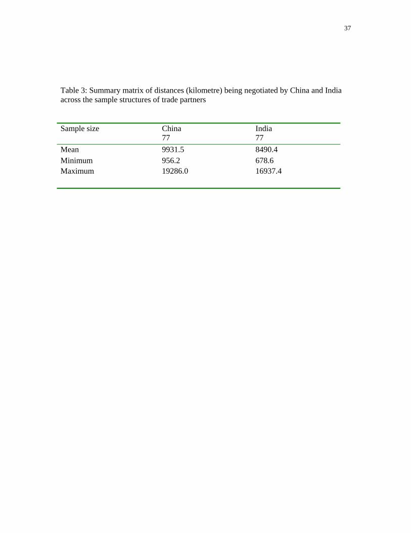
may be noted that the average distance of China from its trading partners is greater than

that of India from its trading partners (Table 3). Therefore, India has to be more efficient

in cost management in order to compete with China in the same product group or else it

has to design alternative strategies related to product and market. For example, empirical

studies examining the costs of doing business in India often have cited that private firms

17 For the purpose of the present study of comparing the performances of China and India emulating the exporting environment of each other, it is necessary to consider the same countries with which both China and India traded during the sample periods.

21

have to have their own power generators in order to avoid the problem of power shortage,

which tend to increase their production costs (Rajan, 2006). Further, China is more

concerned with other barriers to trade rather than distance. For example, in Model CHN-

14 (Table 2), the relative distance variable becomes insignificant, when tariff barrier to

primary sector products is introduced. Also as new variables are added, the coefficient of

relative distance variable in China’s models go on reducing. Therefore, it can be safely

argued that China’s cost advantages are great instruments to boost their exports compared

to India.

The coefficient of size of the economy measured by GDP is consistently significant in all

formulations. The size of this coefficient is larger for China than that for India in both

models. However, when variables such as openness to trade and growth competitiveness

are added in the model, the size of coefficient of GDP reduces for China and India (See

Table 2 in comparison with Table 1). Nevertheless, the coefficient of GDP is larger for

China than for India. This means that clearly India has to go a long way ahead to

manufacture and export premium products consumed in richer countries as compared to

the manufacturing activities in China.

Population is indirectly covered in the size of the economy, it can be argued to have

independent demand side effects also. For example, subsistent economies also need basic

amenities of livelihood such as cheap clothing and food. Countries such as China and

India, which have fairly high degree of mechanised production system with cheap labour

could be potential source of imports provided the importing country has conducive trade

18 The results could have been better, had we disaggregated exports of China and India by commodity categories such as labour-intensive, agriculture-intensive, and resource-intensive. We thank the discussant, Lael Brainard for pointing out this issue.

22

regime. This fact is revealed on comparing the coefficients of population variable across

models.

Openness to trade variable (TRDGZ) is introduced in Models CH14, IN13, and IN14

along with the area variable (Table 2). Clearly, exports flow more from both countries to

those countries, which trade higher proportion of their GDP. The coefficient of TRDGZ

is almost equal for both China and India. In the case of China, GCI is not a significant

variable; instead, tariff barriers to primary sector products are more important in reducing

its exports. Even non-tariff barriers are insignificant in affecting China’s exports. On the

other hand, in the case of India, non-tariff barriers and growth competitiveness index act

alike in affecting its exports growth. It may be recalled that expected sign of coefficient

of NTBI is positive because higher value of NTBI means lesser problems in importing

while lower values mean the opposite.

To calculate potential exports, it is important to estimate the equation in a general

equilibrium framework so that as many trading partners as possible, indicating as much

distances as possible are covered. Nevertheless, such a general equilibrium framework

may not take into account all country-specific characteristics of home country that

influence its exports. Therefore, in this exercise we put each country in the exporting

environment of the other to simulate each other country’s potential exports. The key

difference in export performance is expected to arise due to the change in the values of

the relative distance variable, as all other variables remain more or less the same across

trading countries. Models CHN-14 and IND-14 given in Table 2 were used for

simulating the exports from China and India with the assumption that they switched their

exporting environments between them. Simulations were carried out by applying the

23

coefficient of India, which proxies the exporting environment faced by India, on trade

data concerning China and vice versa. The simulated gain/loss in exports is presented in

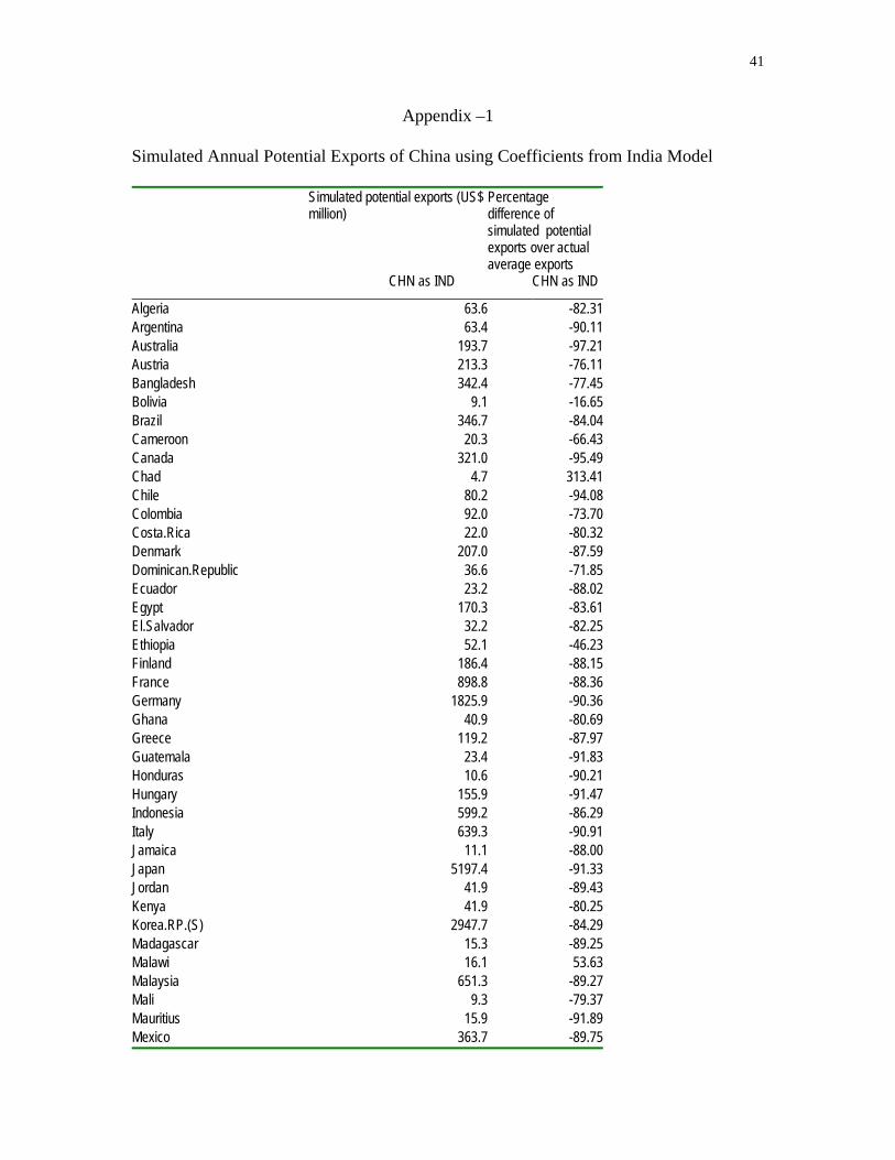
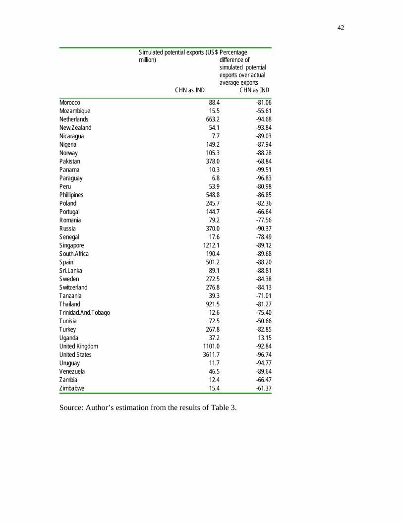
Appendices1 and 2.

As a summary, when the coefficients of China are applied to calculate India’s simulated

potential exports, it results in very high values for India (672.9%) implying that if India

enjoys China’s exporting environment, it would increase its exports drastically. On the

other hand, when India’s coefficients are applied to China, it leads to lowering of exports

from China by 91.7%, clearly indicating that China has been operating at much higher

efficiency levels than India. Thus, there is much for India to learn from China to improve

its export performance. This result also implies that there are significant ‘behind the

border constraints’ to export more in India than in China, which is examined in the next

section.

4.2. Presence of “Behind the border constraints”

The following modified augmented gravity model was estimated using panel data from

2000 to 2003 and the results are presented in Table 4:

ijtijttt

ttjtijtjtijt

uvTNTBITBPR

LAREATRDGZPOPDISGDPX

−++++

+++++=

654

3211 lnlnlnln

δδδ

δδδγβα (7)

The variables are as defined earlier and ‘T’ refers to time, which takes values 1,2, 3,and 4

respectively for data from 2000,2001,2002, and 2003. The variable uij is assumed to be

non-negative truncations of the normal distribution with mean, ,µ and variance, σ2.

Further, the assumption that [ ]{ } ijijitijt uTtuu )(exp −−== ηη means that ‘behind the

border constraints’ to export have been varying over time. This assumption implies that if

the estimate of η , which is provided by the computer program FRONTIER 4.1

24

simultaneously along with the parameters of equation (7), is positive then the ‘behind the

border constraints’ decline exponentially to its minimum value, uij, at the last period, T of

the panel. In this case, the gap between potential and actual exports has been declining.

The coefficient estimates for constant, which is larger than the estimates of equation (6)

as expected due to the specification of equation (7), and most variables are significant at

least at the 5 per cent level. Further, these coefficient estimates have the signs that

concur with the theory. The coefficient γ presents a measure of the total variation that is

due to country specific ‘behind the border constraints’ to export. The γ coefficient is an

average over the time period. That is, γ = [(Σt σ2ut) / (Σt σ2

ut + σ2vt)] / T, where is σ2

ut is

the variance of the one-sided error term at period t, σ2vt is the variance of the random

error term at period t and T is the total number of time periods. The estimate of γ is large

and significant at the 1 per cent level. This means that the decomposition of the error

term into u and v in equation (7) is valid for the present data set and the deviation of

actual exports from potential exports is due to “behind the border constraints” and not by

just random chances. It may be interesting to see how do the γ coefficients vary over

time. This is equivalent to examine whether the influence of ‘behind the border

constraints’ to export within the home country have been decreasing from one period to

another or not. To put it differently, whether policy reforms towards promoting exports

in China and India have been effective during the sample period. Information on the

temporal behaviour of γ can be obtained by examining the η coefficient.

The η coefficient considers whether the impact of country specific ‘behind the

border constraints’ on reaching potential exports have been decreasing from one time

period to another or not. If the η coefficient were positive, then the impact of country

25

specific ‘behind the border constraints’ to export would be decreasing over time. If,

however η were zero or not significant, then the impact of country specific ‘behind the

border constraints’ to export could be considered to be constant over time. In the above

model, the η coefficient is positive and significant for China, while it is positive but not

significant for India. This implies that policy reforms in India do not appear to be

effective in reducing ‘behind the border constraints’ to export during the sample period,

though policy reforms seem to be effective in China.

Overall, from the above results the following can be inferred. ‘Behind the border

constraints’ (measured by “u”) contribute a large and significant proportion to the

variation in the gaps between potential and actual exports in equation (7) for both China

and India. This point is further emphasised by the significance of γ . In other words,

country-specific factors including trade policy are important determinants of potential

and actual exports. The results given in Table 4 indicate that the impact of ‘behind the

border constraints’ to export has reduced over time during the sample period for China

and not for India. With the existing trade resistance between China and its trading

partners, and India and its trading partners, China has been able to reduce the gap

between its potential and actual exports with majority of the member countries more than

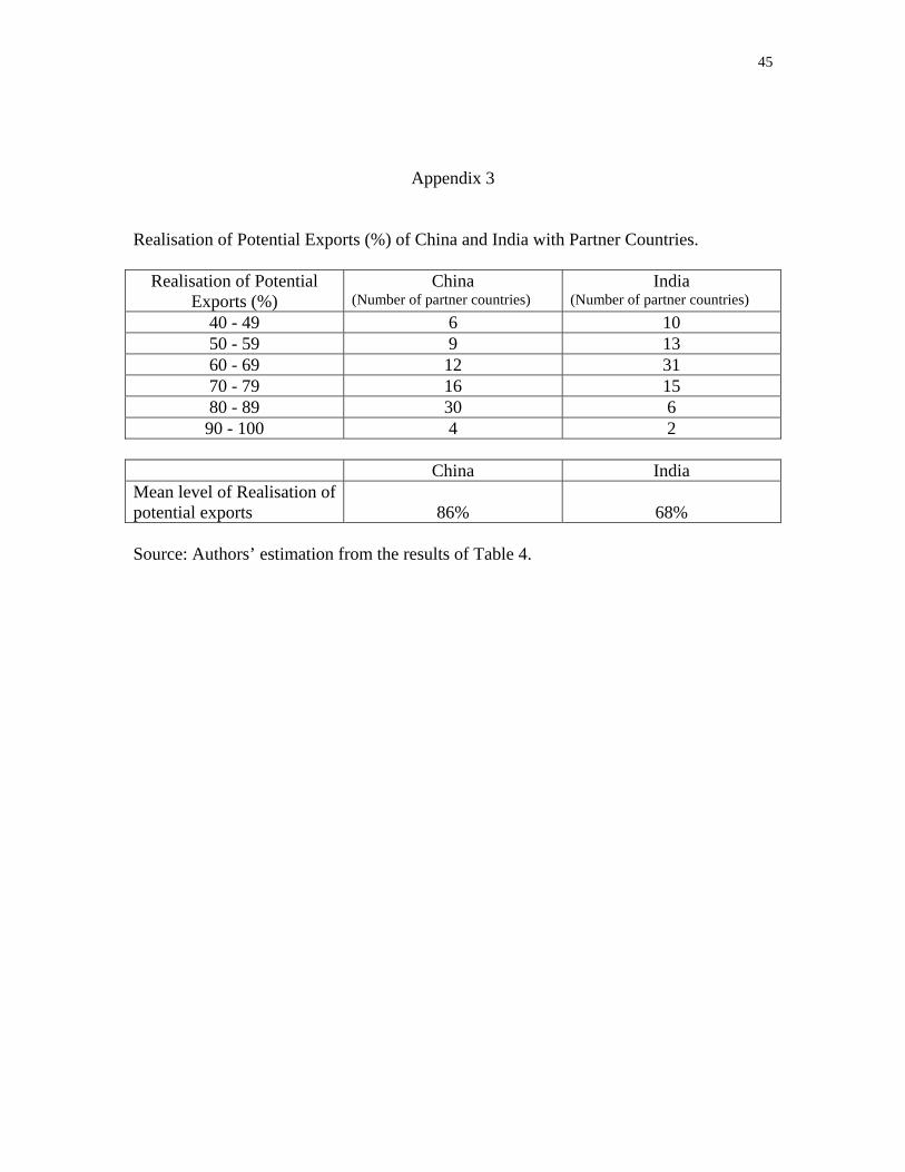
India could do over time. The analysis shows that on an average about 86 percent of

potential exports has been realized by China, while only about 68 percent of potential

exports has been realized by India (Appendix 3). This clearly indicates that there is an

urgent need to design and intensify trade policy reforms to enhance its effectiveness

towards reducing constraints to export in India and in this respect, India certainly can

learn from China’s experience, which requires a detailed study. Nevertheless, India needs

26

to study carefully the recently debated regional income inequality problems created by

China’s surging export revenues in order to avoid the occurrence of such social problems

while increasing India’s exports19.

5. Conclusions

Thus, China’s export performance contrasted with that of India over the years indicate

that an important determinant of the benefits which developing countries can reap from

globalization is whether ‘behind the border constraints’ to export can be decreased

consistently through appropriate policy measures. Though this study did not explore what

kind of ‘behind the border constraints’ need to be eliminated in India to facilitate the

realization of its export potential, conjectures can be made from China’s experience.

Drawing on Hayami (1997) who argued that poor countries could structure their

institutions to bring about rapid development through the borrowing of technologies, the

adoption of technology from abroad is important for India, which appears to be

constrained by mainly lack of infrastructure and proper institutions.

"Catching up with China" is a worthwhile slogan for India's new millennium, along with

a national commitment to grow at 10 percent a year. Both goals may be feasible and

attainable, and within India's grasp, provided infrastructure and institutional reforms are

intensified effectively. China has not only managed a high rate of investment, but has

kept the prime lending rate (PLR) at a relatively low 8 percent; the interest rate spread

between lending and deposit rates was confined to 2.6 per cent. In India, the PLR is 12

per cent, while the interest rate spread is at 3.4 percent. Clearly, China's configurations

are more conducive to high domestic investment. Even though the Indian stock markets

19 We are thankful to Zhang Xiaojing for pointing out this important issue to us.

27

were established much before China's, in terms of market capitalisation, China is ahead at

$231.3 billion, which is 2.20 times that of India's. Chinese banks extend credit, measured

as a ratio of GDP, at a rate of two-and-a-half times India's. Even in fiscal

decentralisation, the Chinese Central government transfers 51.4 percent of the tax

revenue to the provinces, while in India the figure is about 36.1 percent.

The above discussion has revealed important findings, which can be helpful in making

strategies with respect to trade policy in India. The cost competitiveness of China appears

to help its exports in negotiating large distances. India needs to learn from China. It has to

develop cost advantage and product process so that high value markets can be captured.

Duties and taxes are still on the higher side as compared to world standards, and they

need to be reduced further, as higher duties and taxes lead to higher domestic prices and

reduced market size by reducing domestic consumption, and hence deprive the scale-of-

economy effect and make Indian firms less competitive. A larger consumption base will

lead to increase in labour productivity through competition and provide backstop to

domestic producers against external shocks. Duties merit reduction on several other

grounds also. The proven technological potential of the country can best be exploited and

made robust by exposing the economy to external competition by strategically reducing

tariffs. Low-level tariffs have strong signalling effects, besides reducing inefficiencies in

resource allocation and operations. A relatively restrictive foreign investment regime in

India needs review. FDI flows should be viewed as a vehicle of technology transfer,

spillover effects in production processes, and of increasing exports20. Continuation of

small-scale industry reservation in the case of many sectors of production deprives the

28

benefits of scale economy and a strategic decision of de-reservation should be taken for

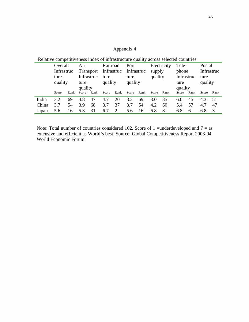
all the products where export potential exists. The poor quality of public infrastructure

including power and transport remains a key problem for business enterprises (See,

Appendix 4). The sooner it is rectified the better and, therefore, it is argued that the

government should continue its efforts in building infrastructure instead of managing

production units. Relatively sluggish clearing at ports and customs houses and rampant

corruption are increasing costs to domestic manufactures and they must be addressed

through technological measures and a greater participation of the private sector. The

state-owned port trust is extremely inefficient and the government has rightly assigned

some responsibilities to international operators recently.

It is not that India has not proved its successful performance in trade sector. As argued by

Rajan (2006) India has proved that it could compete in the services trade sector despite

the poor infrastructure in high-value-added, high-skill industries where the output is

relatively lightweight and relatively less dependent on ports and electricity. For example,

during the 1990s, India’s service sector grew at an average annual rate of 9 percent,

contributing to nearly 60 percent of the overall growth rate of the economy. Further,

India’s exports of services grew annually on average at 17 percent per year in the 1990s,

which is about two and a half times faster than the domestically focused part of the

services sector (Hoekman, 2004).

Thus, it is argued that India should nurture this comparative advantage effectively by

relaxing ‘behind the border constraints’ rather than introducing new constraints such as

over regulation of higher education system. Nevertheless, in order to provide sustained

20 Unlike other studies, which are cross-country based, this study is country-specific (India Vs. its trading partners and China Vs. its trading partners) and therefore, FDI could not be used as an explanatory variable

29

employment to several million people, India can not underestimate the benefits of

following the East Asian growth model of labour intensive manufacturing, which is also

causally linked with the services sector.

in the gravity model estimation.

30

References

Aigner, Dennis, Lovell, Knox, and Schmidt, Peter. 1977. “Formulation and estimation of

stochastic frontier production function models”. Journal of Econometrics 6: 21-37.

Anderson, James. 1979. “A Theoretical Foundation for the Gravity Equation”. American

Economic Review 69: 106-116.

Anderson, James and van Wincoop, Eric. 2003. “Gravity with Gravitas: A Solution to the

Border Puzzle”. American Economic Review 93(1): 170-192.

Baldwin, R. 1994. Towards an Integrated Europe. London: CEPR.

Baldwin, R. 2003. ‘Openness and Growth: What’s the Empirical Relationship?’ NBER

Working Paper 9578, Cambridge MA.

Bergstrand, J. H. (1985), “The Gravity Equation in International Trade: Some

Microeconomic Foundations and Empirical Evidence.” The Review of Economics and

Statistics 67: 478- 481.

Bhagwati, Jagdish. 1993. India in Transition: Freeing the Economy. Oxford: Oxford

University Press.

Chadha, Rajesh. 2003. External Sector in N.N. Vohra (ed). Mid-Year Review of the

Indian Economy 2002-2003. New Delhi:Shipra publishing.

China Custom Statistical Bureau. 2002. China Custom Statistical Yearbook. Beijing.

Coelli, Tim. 1996. ‘A guide to FONTIER version 4.1: A computer program for stochastic

frontier production and cost function estimation’. Centre for Efficiency and Productivity

Analysis Working Paper 96/07, University of New England, Armidale.

Drysdale, Peter, Huang, Yiping, and Kalirajan, Kaliappa. 2000. ‘China’s Trade

Efficiency: Measurement and Determinants’ in Peter Drysdale, Zhang Yunling, and

31

Liagang Song (eds.) APEC and Liberalisation of the Chinese Economy. Canberra: Asia

Pacific Press.

Frankel, J.A. and D. Romer. 1999. “Does Trade Cause Growth?” American Economic

Review 89(3): 379-99.

Gang Fan and Xiaojing Zhang 2003. ‘The Chinese Reform Agenda’ in J.J. Teunissen in

China’s Role in Asia and the World Economy - Fostering Stability and Growth, Fondad,

The Hague.

Garnaut, Ross and Yiping Huang 2001.Growth Without Miracles: Readings on the

Chinese Economy in the Era of Reform. New York: Oxford University Press .

Gawande, K. and Krishna, P. 2001. ‘The Political Economy of Trade Policy: Empirical

Approaches’. Working Papers, Economics Department, Brown University.

Greenaway, D., W. Morgan and P. Wright (2002). “Trade Liberalization and Growth in

Developing Countries”. Journal of Development Economics 67: 229-44.

Hayami, Yujiro. 1997. Development Economics: From the Poverty to the Wealth of Nations, Oxford: Clarendon Press.

Hoekman, Bernard. 2004. ‘The World Bank Trade Research Program: Summary and Synthesis’. Development Economics Research Group (DECRG), Washington, D.C. :The World Bank. Huang, Yasheng, and Khanna, Tarun. 2003. Can India Overtake China? Foreign Policy

Magazine, July-August 2003 URL: http://www.foreignpolicy.com/story/.

Jiang Xiaojuan, 2002, The Foreign Invested Sector in China: its contribution to economic

growth, structure upgrade and power of competitiveness. People’s University Press,

Beijing.

Kalirajan, Kaleeswaran. 1999. “Stochastic Varying Coefficients gravity model: an

approach in trade analysis”. Journal of Applied Statistics 26(2): 185-193.

32

Kalirajan, Kaliappa. 2000. “Indian Ocean Rim Association for Regional Cooperation

(IOR-ARC): Impact on Australia’s Trade”, Journal of Economic Integration 15: 533-

547.

Kalirajan, Kaliappa. 2007. “Regional Cooperation and Bilateral Trade Flows: An

Empirical Measurement of Resistance”, The International Trade Journal XXI: 85-107.

Lardy, Nicholas. 2002. Integrating China into the Global Economy. Washington:

Brookings Institution Press.

Levchenko, A. A. 2004. ‘Institutional Quality and International Trade’. IMF Working

Paper, WP/04/23.

Lucas, Robert. 1988. “On the mechanics of economic development”. Journal of

Monetary Economics 22: 3–42.

Mayer J. 2000. ‘Globalization, technology transfer, and skill accumulation in low-income

countries’. Discussion Paper, No. 150. Geneva: UNCTAD.

Meeusen, William. and van den Broeck, Julian. 1977. “Efficiency estimation from Cobb

Douglas production function with composed error”. International Economic Review 18:

435-444.

NBS(a) (National Statistical Bureau), various years. China Statistical Yearbook. China

Statistics Press, Beijing.

NBS(b) (National Statistical Bureau), various years. China Foreign Economic Statistical

Yearbook. China Statistics Press, Beijing.

Nilsson, L. 2000. “Trade integration and the EU economic membership criteria”.

European journal of Political Economy. 16(4): 807-827.

33

Rajan, Raghuram. 2006. “India: The Past and its Future”. Asian Development Review

23(2): 36-52.

Roberts, Mark and Setterfield, Mark 2006. ‘What is endogenous growth?’, in P. Arestis,

M. Baddeley and J. S. L. McCombie (Eds) Understanding Economic Growth. New

Directions in Theory and Policy. Cheltenham: Edward Elgar.

Rodrik, Danny. 1998. “Why Do More Open Countries Have Large Governments?”

Journal of Political Economy 106 (5): 758-879.

Rodrik, Danny. 2000. Trade Policy as Institutional Reform, Harvard University,

Department of Economics, Cambridge, Mass.

Roemer, J.E. 1977. “The effect of sphere of influence and economic distance on the

commodity composition of trade in manufactures”. The Review of Economics and

Statistics 59: 318-27.

Romer, Paul. 1986. “Increasing returns and long-run growth”. Journal of Political

Economy 94: 1002–1037.

Sachs, Jeffery, and Woo, Wing Thye. 2002. “China's Economic Growth After WTO

Membership”. Journal of Chinese Economic and Business Studies, Volume 1.

Sachs, Jeffrey, and Warner, A. 1995. “Economic Reform and the Process of Global

Integration”. Brookings Papers on Economic Activity 1: 1-95.

Sachs, Jeffrey, and Woo, Wing Thye 2000. “Understanding China’s Economic

Performance”. Journal of Policy Reform 4(1).

Sachs, Jeffrey, and Woo, Wing Thye. 2002. “China's Economic Growth After WTO

Membership”. Journal of Chinese Economic and Business Studies 1.

34

Sala-i-Martin, Xavier. 2004. The Global Competitiveness Report 2003-04. New York:

Oxford University press.

Wacziarg, R. 1997. Trade, Competition and Market Size. Cambridge, Mass: Harvard

University Press.

Wang, Xiaolu. 2004. ‘FDI in People’s Republic of China’ in D. H. Brooks and H. Hill

(eds): Managing FDI in a Globalizing Economy: Asian Experiences. pp.79-117. London:

Palgrave/MacMillan.

Woo, Wing Thye. 1998. ‘Chinese Economic Growth: Sources and Prospects’ in Michel

Fouquin and Francoise Lemoine (ed.). The Chinese Economy. London:Economica.

World Bank. 2003. World Development Report 2003: Sustainable Development in a

Dynamic World, Washington, D.C.: Oxford University Press.

Wu, J. L. 2003. Economic Reform in Contemporary China. Shanghai: Shanghai Far East

Press.

35

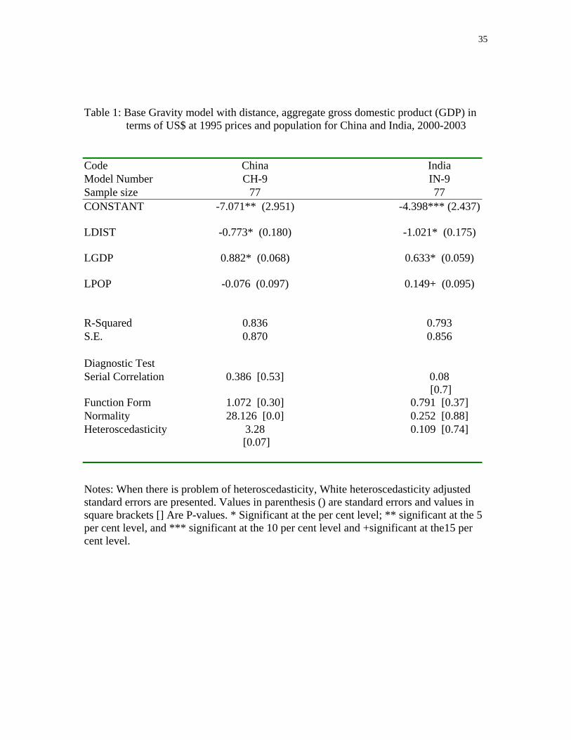
Table 1: Base Gravity model with distance, aggregate gross domestic product (GDP) in

terms of US$ at 1995 prices and population for China and India, 2000-2003 Code China India Model Number CH-9 IN-9 Sample size 77 77 CONSTANT -7.071** (2.951) -4.398*** (2.437)

LDIST -0.773* (0.180) -1.021* (0.175)

LGDP 0.882* (0.068) 0.633* (0.059)

LPOP -0.076 (0.097) 0.149+ (0.095)

R-Squared 0.836 0.793 S.E. 0.870 0.856

Diagnostic Test Serial Correlation 0.386 [0.53] 0.08

[0.7] Function Form 1.072 [0.30] 0.791 [0.37] Normality 28.126 [0.0] 0.252 [0.88] Heteroscedasticity 3.28

[0.07] 0.109 [0.74]

Notes: When there is problem of heteroscedasticity, White heteroscedasticity adjusted standard errors are presented. Values in parenthesis () are standard errors and values in square brackets [] Are P-values. * Significant at the per cent level; ** significant at the 5 per cent level, and *** significant at the 10 per cent level and +significant at the15 per cent level.

36

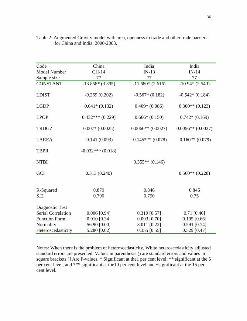
Table 2: Augmented Gravity model with area, openness to trade and other trade barriers

for China and India, 2000-2003. Code China India India Model Number CH-14 IN-13 IN-14 Sample size 77 77 77 CONSTANT -13.858* (3.395) -11.680* (2.616) -10.94* (2.540)

LDIST -0.269 (0.202) -0.567* (0.182) -0.542* (0.184)

LGDP 0.641* (0.132) 0.409* (0.086) 0.300** (0.123)

LPOP 0.432*** (0.229) 0.666* (0.150) 0.742* (0.169)

TRDGZ 0.007* (0.0025) 0.0060** (0.0027) 0.0056** (0.0027)

LAREA -0.141 (0.093) -0.145*** (0.078) -0.160** (0.079)

TBPR -0.032*** (0.018)

NTBI 0.355** (0.146)

GCI 0.313 (0.240) 0.560** (0.228)

R-Squared 0.870 0.846 0.846 S.E. 0.790 0.750 0.75

Diagnostic Test Serial Correlation 0.006 [0.94] 0.319 [0.57] 0.71 [0.40] Function Form 0.910 [0.34] 0.093 [0.70] 0.195 [0.66] Normality 56.90 [0.00] 3.011 [0.22] 0.591 [0.74] Heteroscedasticity 5.280 [0.02] 0.355 [0.55] 0.529 [0.47] Notes: When there is the problem of heteroscedasticity, White heteroscedasticity adjusted standard errors are presented. Values in parenthesis () are standard errors and values in square brackets [] Are P-values. * Significant at the1 per cent level; ** significant at the 5 per cent level, and *** significant at the10 per cent level and +significant at the 15 per cent level.

37

Table 3: Summary matrix of distances (kilometre) being negotiated by China and India across the sample structures of trade partners Sample size China

77 India 77

Mean 9931.5 8490.4 Minimum 956.2 678.6 Maximum 19286.0 16937.4

38

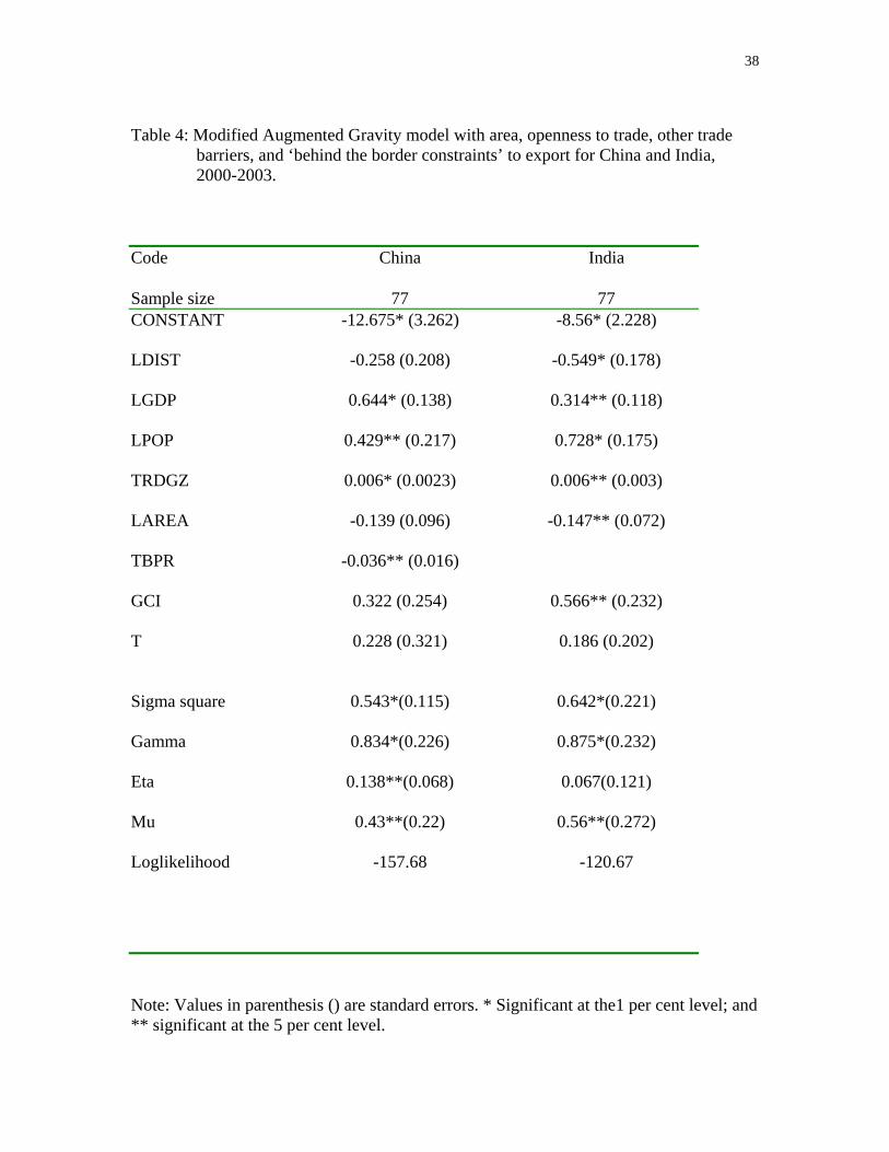
Table 4: Modified Augmented Gravity model with area, openness to trade, other trade

barriers, and ‘behind the border constraints’ to export for China and India, 2000-2003.

Code China India Sample size 77 77 CONSTANT -12.675* (3.262) -8.56* (2.228)

LDIST -0.258 (0.208) -0.549* (0.178)

LGDP 0.644* (0.138) 0.314** (0.118)

LPOP 0.429** (0.217) 0.728* (0.175)

TRDGZ 0.006* (0.0023) 0.006** (0.003)

LAREA -0.139 (0.096) -0.147** (0.072)

TBPR -0.036** (0.016)

GCI T Sigma square Gamma Eta Mu Loglikelihood

0.322 (0.254)

0.228 (0.321)

0.543*(0.115)

0.834*(0.226)

0.138**(0.068)

0.43**(0.22)

-157.68

0.566** (0.232)

0.186 (0.202)

0.642*(0.221)

0.875*(0.232)

0.067(0.121)

0.56**(0.272)

-120.67

Note: Values in parenthesis () are standard errors. * Significant at the1 per cent level; and ** significant at the 5 per cent level.

39

Figure 1: Pattern of Economic Growth of India

-8

-6

-4

-2

0

2

4

6

8

10

12

1951

-52

1953

-54

1955

-56

1957

-58

1959

-60

1961

-62

1963

-64

1965

-66

1967

-68

1969

-70

1971

-72

1973

-74

1975

-76

1977

-78

1979

-80

1981

-82

1983

-84

1985

-86

1987

-88

1989

-90

1991

-92

1993

-94

1995

-96

1997

-98

1999

-00

2001

-02

2003

-04(

A)

Perc

enta

ge G

row

th

Dro ught

Cap ital intens ive Firs t 5-ear p lan, String ent fiscal F-Exchange co ntro l

Droug ht, Nehru & Shatri d ied , War, Hig h Fiscal d eficit ,US aid susp ended

War, Oil Prices , Droug ht, Current A/C deficit , Monetary t ightening

Droug ht, Oil Cris is , Current A/C d eficit

Gulf War, Oil Prices , Fiscal Deficit , Current A/C deficit

Eas t As ian Cris is (9 7), Econo mic Refo rms , Econo mic Sanct ions (98 ), Karg il war, 9 /11/01 attack & Glo bal Slow Do wn, Swelling Fiscal deficit

Dro ught

TG = 3.8 TG = 3.5 TG = 5.4TG = 3.6TG = 6.2

Dro ught

y&

40

Figure 2: Trade reforms in terms of tariff policy across selected countries

0

20

40

60

80

100

120

1990

1999

1992

2000

1989

2000

1990

2000

1988

1997

1989

1999

1989

2000

1989

2000

India China Brazil Sri Lanka Malaysia S. Korea Japan USA

Perc

enta

ge

All product simple mean Standard deviationMFG simple mean Share of lines with international peak

Source: World Development Indicator, 2002

41

Appendix –1

Simulated Annual Potential Exports of China using Coefficients from India Model Simulated potential exports (US$

million) Percentage difference of simulated potential exports over actual average exports

CHN as IND CHN as IND

Algeria 63.6 -82.31Argentina 63.4 -90.11Australia 193.7 -97.21Austria 213.3 -76.11Bangladesh 342.4 -77.45Bolivia 9.1 -16.65Brazil 346.7 -84.04Cameroon 20.3 -66.43Canada 321.0 -95.49Chad 4.7 313.41Chile 80.2 -94.08Colombia 92.0 -73.70Costa.Rica 22.0 -80.32Denmark 207.0 -87.59Dominican.Republic 36.6 -71.85Ecuador 23.2 -88.02Egypt 170.3 -83.61El.Salvador 32.2 -82.25Ethiopia 52.1 -46.23Finland 186.4 -88.15France 898.8 -88.36Germany 1825.9 -90.36Ghana 40.9 -80.69Greece 119.2 -87.97Guatemala 23.4 -91.83Honduras 10.6 -90.21Hungary 155.9 -91.47Indonesia 599.2 -86.29Italy 639.3 -90.91Jamaica 11.1 -88.00Japan 5197.4 -91.33Jordan 41.9 -89.43Kenya 41.9 -80.25Korea.RP.(S) 2947.7 -84.29Madagascar 15.3 -89.25Malawi 16.1 53.63Malaysia 651.3 -89.27Mali 9.3 -79.37Mauritius 15.9 -91.89Mexico 363.7 -89.75

42

Simulated potential exports (US$ million)

Percentage difference of simulated potential exports over actual average exports

CHN as IND CHN as IND

Morocco 88.4 -81.06Mozambique 15.5 -55.61Netherlands 663.2 -94.68New.Zealand 54.1 -93.84Nicaragua 7.7 -89.03Nigeria 149.2 -87.94Norway 105.3 -88.28Pakistan 378.0 -68.84Panama 10.3 -99.51Paraguay 6.8 -96.83Peru 53.9 -80.98Phillipines 548.8 -86.85Poland 245.7 -82.36Portugal 144.7 -66.64Romania 79.2 -77.56Russia 370.0 -90.37Senegal 17.6 -78.49Singapore 1212.1 -89.12South.Africa 190.4 -89.68Spain 501.2 -88.20Sri.Lanka 89.1 -88.81Sweden 272.5 -84.38Switzerland 276.8 -84.13Tanzania 39.3 -71.01Thailand 921.5 -81.27Trinidad.And.Tobago 12.6 -75.40Tunisia 72.5 -50.66Turkey 267.8 -82.85Uganda 37.2 13.15United Kingdom 1101.0 -92.84United States 3611.7 -96.74Uruguay 11.7 -94.77Venezuela 46.5 -89.64Zambia 12.4 -66.47Zimbabwe 15.4 -61.37 Source: Author’s estimation from the results of Table 3.

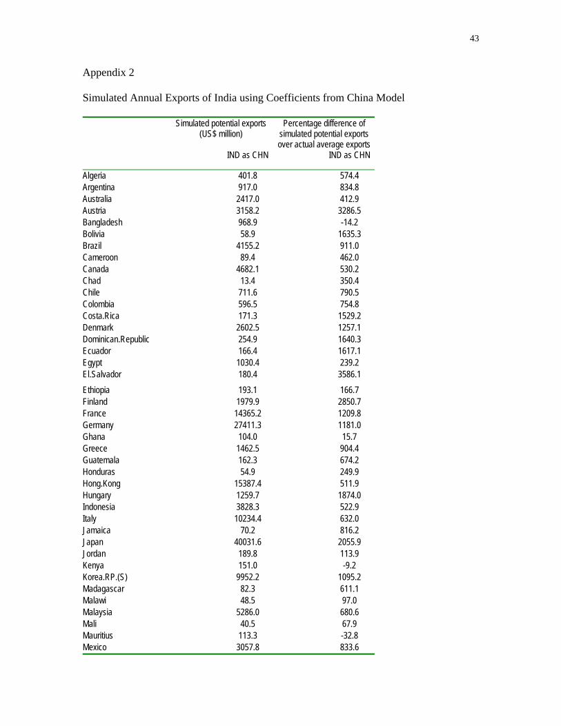
43

Appendix 2

Simulated Annual Exports of India using Coefficients from China Model Simulated potential exports

(US$ million) Percentage difference of

simulated potential exports over actual average exports

IND as CHN IND as CHN

Algeria 401.8 574.4 Argentina 917.0 834.8 Australia 2417.0 412.9 Austria 3158.2 3286.5 Bangladesh 968.9 -14.2 Bolivia 58.9 1635.3 Brazil 4155.2 911.0 Cameroon 89.4 462.0 Canada 4682.1 530.2 Chad 13.4 350.4 Chile 711.6 790.5 Colombia 596.5 754.8 Costa.Rica 171.3 1529.2 Denmark 2602.5 1257.1 Dominican.Republic 254.9 1640.3 Ecuador 166.4 1617.1 Egypt 1030.4 239.2 El.Salvador 180.4 3586.1 Ethiopia 193.1 166.7 Finland 1979.9 2850.7 France 14365.2 1209.8 Germany 27411.3 1181.0 Ghana 104.0 15.7 Greece 1462.5 904.4 Guatemala 162.3 674.2 Honduras 54.9 249.9 Hong.Kong 15387.4 511.9 Hungary 1259.7 1874.0 Indonesia 3828.3 522.9 Italy 10234.4 632.0 Jamaica 70.2 816.2 Japan 40031.6 2055.9 Jordan 189.8 113.9 Kenya 151.0 -9.2 Korea.RP.(S) 9952.2 1095.2 Madagascar 82.3 611.1 Malawi 48.5 97.0 Malaysia 5286.0 680.6 Mali 40.5 67.9 Mauritius 113.3 -32.8 Mexico 3057.8 833.6

44

Simulated potential exports (US$ million)

Percentage difference of simulated potential exports over actual average exports

IND as CHN IND as CHN

Morocco 295.0 331.5 Mozambique 60.2 47.4 Netherlands 9688.7 925.4 New.Zealand 611.2 721.1 Nicaragua 43.0 1725.0 Nigeria 469.9 28.2 Norway 1401.1 1759.7 Pakistan 1962.5 885.1 Panama 82.1 134.3 Paraguay 61.5 704.7 Peru 338.1 861.5 Phillipines 2308.9 695.0 Poland 2004.6 1434.3 Portugal 1655.4 965.9 Romania 477.3 1343.1 Russia 3162.9 392.0 Senegal 92.0 227.4 Singapore 15646.4 1193.6 South.Africa 1996.9 424.8 Spain 6681.6 785.7 Sri.Lanka 425.4 -45.6 Sweden 3210.8 1626.6 Switzerland 3121.1 753.4 Tanzania 117.9 8.7 Thailand 5243.0 698.9 Trinidad.And.Tobago 114.8 843.6 Tunisia 245.6 382.2 Turkey 2353.7 471.8 Uganda 160.7 156.8 United Kingdom 14061.0 453.9 United States 50080.9 388.1 Uruguay 139.0 479.7 Venezuela 377.5 944.5 Zambia 54.9 95.9 Zimbabwe 93.2 510.7 Source: Author’s estimation from the results of Table 3.

45

Appendix 3 Realisation of Potential Exports (%) of China and India with Partner Countries.

Realisation of Potential Exports (%)

China (Number of partner countries)

India (Number of partner countries)

40 - 49 6 10 50 - 59 9 13 60 - 69 12 31 70 - 79 16 15 80 - 89 30 6 90 - 100 4 2

China India Mean level of Realisation of potential exports

86%

68%

Source: Authors’ estimation from the results of Table 4.

46

Appendix 4 Relative competitiveness index of infrastructure quality across selected countries Overall

Infrastructure quality

Air Transport Infrastructure quality

Railroad Infrastructure quality

Port Infrastructure quality

Electricity supply quality

Tele-phone Infrastructure quality

Postal Infrastructure quality

Score Rank Score Rank Score Rank Score Rank Score Rank Score Rank Score Rank

India 3.2 69 4.8 47 4.7 20 3.2 69 3.0 85 6.0 45 4.3 51 China 3.7 54 3.9 68 3.7 37 3.7 54 4.2 60 5.4 57 4.7 47 Japan 5.6 16 5.3 31 6.7 2 5.6 16 6.8 8 6.8 6 6.8 3 Note: Total number of countries considered 102. Score of 1 =underdeveloped and 7 = as extensive and efficient as World’s best. Source: Global Competitiveness Report 2003-04, World Economic Forum.