UNIVERSITY OF CALIFORNIA, SAN DIEGO

A Combinatorial Comparison of Elliptic Curves andCritical Groups of Graphs

A dissertation submitted in partial satisfaction of the

requirements for the degree

Doctor of Philosophy

in

Mathematics

by

Gregg Joseph Musiker

Committee in charge:

Professor Adriano Garsia, ChairProfessor Ronald GrahamProfessor Russell ImpagliazzoProfessor Harold StarkProfessor Nolan Wallach

2007

Copyright

Gregg Joseph Musiker, 2007

All rights reserved.

The dissertation of Gregg Joseph Musiker is ap-

proved, and it is acceptable in quality and form

for publication on microfilm:

Chair

University of California, San Diego

2007

iii

To the memory of my Grandparents Bette and Philip Rosenthal

who continue to inspire me.

iv

TABLE OF CONTENTS

Signature Page . . . . . . . . . . . . . . . . . . . . . . . . . . . . . . . . iii

Dedication . . . . . . . . . . . . . . . . . . . . . . . . . . . . . . . . . . . iv

Table of Contents . . . . . . . . . . . . . . . . . . . . . . . . . . . . . . . v

List of Figures . . . . . . . . . . . . . . . . . . . . . . . . . . . . . . . . . vii

List of Tables . . . . . . . . . . . . . . . . . . . . . . . . . . . . . . . . . viii

Acknowledgements . . . . . . . . . . . . . . . . . . . . . . . . . . . . . . ix

Vita and Publications . . . . . . . . . . . . . . . . . . . . . . . . . . . . x

Abstract of the Dissertation . . . . . . . . . . . . . . . . . . . . . . . . . xi

1 Introduction . . . . . . . . . . . . . . . . . . . . . . . . . . . . . . . . . . 11.1 Background on algebraic curves . . . . . . . . . . . . . . . . . . . . 21.2 Combinatorial definition of primes . . . . . . . . . . . . . . . . . . . 41.3 The Riemann-Roch theorem and rationality of the zeta function . . 91.4 The Weil conjectures . . . . . . . . . . . . . . . . . . . . . . . . . . 201.5 Introduction to symmetric functions . . . . . . . . . . . . . . . . . . 22

2 The zeta function and symmetric functions . . . . . . . . . . . . . . . . . 262.1 Rewriting the zeta function via plethysm . . . . . . . . . . . . . . . 272.2 Plethysm with a different alphabet . . . . . . . . . . . . . . . . . . 282.3 Egecioglu and Remmel’s combinatorial interpretation of formula (2.5) 312.4 Alternative to plethysm . . . . . . . . . . . . . . . . . . . . . . . . 332.5 An inclusion-exclusion interpretation for (2.5) . . . . . . . . . . . . 36

3 Elliptic curves . . . . . . . . . . . . . . . . . . . . . . . . . . . . . . . . . 383.1 Weierstraß form and group law . . . . . . . . . . . . . . . . . . . . 383.2 Rational function representations of morphisms . . . . . . . . . . . 433.3 Division polynomials and the multiplication by n map . . . . . . . . 483.4 Further properties of the Frobenius map . . . . . . . . . . . . . . . 52

4 Combinatorial aspects of elliptic curves . . . . . . . . . . . . . . . . . . . 554.1 First answer to Question 4.2 . . . . . . . . . . . . . . . . . . . . . . 56

4.1.1 The Lucas numbers and a (q, t)-analogue . . . . . . . . . . . 564.1.2 (q, t)−Wheel numbers . . . . . . . . . . . . . . . . . . . . . 614.1.3 First proof of Theorem 4.13: Bijective . . . . . . . . . . . . 63

v

4.1.4 Second proof of Theorem 4.13: Via generating function iden-tities . . . . . . . . . . . . . . . . . . . . . . . . . . . . . . . 66

4.2 More on bivariate Fibonacci polynomials via duality . . . . . . . . . 684.2.1 Duality between the symmetric functions hk and ek . . . . . 684.2.2 Duality between Lucas and Fibonacci numbers . . . . . . . . 72

4.3 Case-Study on N2 = (2 + 2q)N1 −N21 . . . . . . . . . . . . . . . . . 76

4.3.1 Algebraic proof . . . . . . . . . . . . . . . . . . . . . . . . . 794.3.2 The explicit bijection . . . . . . . . . . . . . . . . . . . . . . 804.3.3 Determining when there is an isomorphism . . . . . . . . . . 86

4.4 Geometric interpretations of fractions Nk/N1 . . . . . . . . . . . . . 944.5 Acknowledgement . . . . . . . . . . . . . . . . . . . . . . . . . . . . 101

5 Determinantal formulas for Nk . . . . . . . . . . . . . . . . . . . . . . . . 1025.1 First proof of Theorem 5.1: Via graph theory . . . . . . . . . . . . 103

5.1.1 The Smith normal form of matrices Mk . . . . . . . . . . . . 1055.2 Second proof of Theorem 5.1: Using orthogonal polynomials . . . . 110

5.2.1 Explicit connection to orthogonal polynomials . . . . . . . . 1125.3 Third proof of Theorem 5.1: Using the zeta function . . . . . . . . 116

5.3.1 Combinatorics of elliptic cyclotomic polynomials . . . . . . . 1195.3.2 Geometric interpretation of elliptic cyclotomic polynomials . 124

5.4 Acknowledgement . . . . . . . . . . . . . . . . . . . . . . . . . . . . 125

6 Connections between elliptic curves and chip-firing . . . . . . . . . . . . 1266.1 Introduction to chip-firing games . . . . . . . . . . . . . . . . . . . 1266.2 Connection to elliptic curves . . . . . . . . . . . . . . . . . . . . . . 128

6.2.1 Group structure . . . . . . . . . . . . . . . . . . . . . . . . . 1306.2.2 Analogues of elliptic cyclotomic polynomials . . . . . . . . . 133

6.3 Characterization of critical configurations . . . . . . . . . . . . . . . 1366.4 Connections to deterministic finite automata . . . . . . . . . . . . . 1406.5 Another kind of zeta function . . . . . . . . . . . . . . . . . . . . . 1426.6 Conclusions and topics for further research . . . . . . . . . . . . . . 144

References . . . . . . . . . . . . . . . . . . . . . . . . . . . . . . . . . . . . . 146

vi

LIST OF FIGURES

Figure 4.1: Illustrating proof of Proposition 4.5. . . . . . . . . . . . . 59Figure 4.2: Illustrating definition of Wn(q, t). . . . . . . . . . . . . . . 62Figure 4.3: Illustrating bijection of Theorem 4.13. . . . . . . . . . . . 64

Figure 5.1: A second definition of Wk(q, t). . . . . . . . . . . . . . . . 103

Figure 6.1: Illustrating Propositions 6.9 and 6.10. . . . . . . . . . . . 135Figure 6.2: Deterministic finite automaton MG. . . . . . . . . . . . . . 141

vii

LIST OF TABLES

Table 2.1: Correspondence between algebraic geometric quantities andsymmetric functions. . . . . . . . . . . . . . . . . . . . . . . . . . . 31

Table 2.2: Cyclotomic polynomials Cycd(x) for selected d. . . . . . . . 35

Table 4.1: Nk’s as polynomials for small k. . . . . . . . . . . . . . . . 55Table 4.2: Ek, i.e. F2k−1(q, t)’s for small k for the special case of an

elliptic curve. . . . . . . . . . . . . . . . . . . . . . . . . . . . . . . 69Table 4.3: Plethysm of ek, hk for elliptic curves. . . . . . . . . . . . . 71Table 4.4: Plethystic dictionary for elliptic curves and spanning trees. 72

Table 5.1: Elliptic cyclotomic polynomials ECyck(q,N1) for small k. . 120

Table 6.1: The polynomials WCycd(q, t) for small d. . . . . . . . . . . 133

viii

ACKNOWLEDGEMENTS

First, with much appreciation I thank my advisor, Adriano Garsia, for his

guidance, continual enthusiasm, and unwavering dedication over the last five years.

Adriano has taught me a variety of beautiful mathematical topics, and his passion

for mathematics, the beach, and life in general has been quite contagious. I am also

indebted to Nolan Wallach for aiding me in my studies of representation theory

and algebraic geometry, and appreciate his invaluable feedback during my graduate

school. Many other professors have helped me along my journey, and while I can’t

name them all, I wanted to especially thank Wee Tak Gan, Allen Knutson, Jim

Propp, Christophe Reutenauer, Harold Stark, William Stein, and Richard Stanley.

I am thankful to Sam Buss and Jim Lin for their dedication as Chair and Vice-Chair

and their work initiating new opportunities and support for graduate students; as

well as the excellent staff of the UCSD Mathematics Department, especially Lois

Stewart, Wilson Cheung, and Yi Ling Ng. Additionally, I would like to thank the

San Diego Chapter of the ARCS Foundation for their financial support during my

graduate school.

My colleagues and friends, Jason Bandlow, Arthur Berg, Dave Clark, Mark

Colarusso, Eric Tressler, Jake Wildstrom, Aaron Wong, Scott Cohen, Rick Capella,

Andrew Cosand, German Eichberger, Emmi Olson, Jeff Gold, Emily Anderson,

Lee Lovejoy, and countless others, thank you all for enriching my graduate school

experience with technical and moral support, as well as frisbee, poker, and many

good meals. Most of all, I would like to thank my parents Brian and Lori Musiker

for always inspiring me to learn. This thesis is only possible because of their

continual love, advice, and support.

Much of the material in Chapter 4 and 5 has been submitted for publication

in the paper “Combinatorial Aspects of Elliptic Curves“ by Gregg Musiker. The

dissertation author is the primary investigator and author of this paper.

ix

VITA

1980 Born, Philadelphia, Pennsylvania

2002 B. A., magna cum laude, Harvard University

2002–2006 Teaching assistant, Department of Mathematics, Uni-versity of California San Diego

2004 M. A., University of California San Diego

2006 Associate Instructor, Department of Mathematics,University of California San Diego

2007 Ph. D., University of California San Diego

PUBLICATIONS

J. Bandlow and G. Musiker. Quasi-invariants of S3. J. Combin. Theory Ser. A109 (2005), no 2, 281-298.

G. Musiker and J. Propp. Combinatorial Interpretations for Rank-Two ClusterAlgebras of Affine Type. Electronic Journal of Combinatorics. 14 (2007), no R15,1-23.

A. Garsia and G. Musiker. Basics on Hyperelliptic Curves over Finite Fields.Mongraphies du LaCIM. (To appear.)

G. Musiker. Combinatorial Aspects of Elliptic Curves. (Submitted.)

x

ABSTRACT OF THE DISSERTATION

A Combinatorial Comparison of Elliptic Curves and

Critical Groups of Graphs

by

Gregg Joseph Musiker

Doctor of Philosophy in Mathematics

University of California San Diego, 2007

Professor Adriano Garsia, Chair

In this thesis, we explore elliptic curves from a combinatorial viewpoint. Given

an elliptic curve E, we study here Nk = #E(Fqk), the number of points of E

over the finite field Fqk . This sequence of numbers, as k runs over positive in-

tegers, has numerous remarkable properties of a combinatorial flavor in addi-

tion to the usual number theoretical interpretations. In particular we prove that

Nk = −Wk(q, t)|t=−N1 where Wk(q, t) is a (q, t)-analogue for the number of span-

ning trees of the wheel graph. Additionally we develop a determinantal formula for

Nk where the eigenvalues can be explicitly written in terms of q, N1, and roots of

unity. We also discuss here a new sequence of bivariate polynomials related to the

factorization of Nk, which we refer to as elliptic cyclotomic polynomials because

of their various properties.

The above formula for Nk in terms of Wk motivates a closer examination of

the relationship between points on an elliptic curve E over Fqk and spanning trees

on the wheel graph Wk. An elliptic curve E has an abelian group structure, and

indeed the set of spanning trees of a graph also has an abelian group structure.

Here we study one isomorphic to the critical group of the graph, which has ties to

the theory of chip-firing games and abelian sandpile models of dynamical systems.

While we first focus on the relationship between the integer sequences {Nk} and

{Wk(q,N1)}, we also compare these two group structures, illustrating that the

xi

connections between elliptic curves and spanning trees run even deeper. Numerous

theorems which are true for elliptic curve groups have analogues in terms of critical

groups of the (q, t)-wheel graph.

Additionally, the theory of critical groups will also allow us to re-interpret the

group elements as the set of admissible words for a primitive circuit in a specific

deterministic finite automaton. As an application, we will then compare the zeta

function of an elliptic curve and the zeta function of the corresponding cyclic

language.

xii

1 Introduction

An interesting problem at the cross-roads between combinatorics, number the-

ory, and algebraic geometry is that of counting the number of points on an al-

gebraic curve over a finite field. Over a finite field, the locus of solutions to an

algebraic equation is a discrete subset, but since they satisfy a certain type of

algebraic equation this imposes a lot of extra structure below the surface. One of

the ways to detect this additional structure is by observing that considering field

extensions, the infinite sequence of cardinalities is only dependent on a finite set

of data. Specifically we let Fq denote the unique finite field, up to isomorphism,

which has q elements. Since q is the size of this field, q must be a power of a prime,

e.g. pℓ, and finite algebraic extensions of this field will result in fields with qk = pℓk

elements. In the case of a genus g algebraic curve, the number of points over Fq,

Fq2 , . . . , and Fqg will be sufficient data to determine the number of points over any

other algebraic field extension.

This observation motivates the question of how the points over higher field

extensions relate to points over the first g extensions. In this thesis we explore

this question from a combinatorial point of view. We begin with background on

algebraic curves which includes standard algebraic geometric terminology. This

will include a definition of the zeta function, which is an exponential generating

function defined by considering the sequence of numbers given by the cardinalities

over various extension fields. We will then switch gears, and in Chapter 2 discuss a

more combinatorial way to approach this problem and include connections to the

theory of symmetric functions.

Afterwards, we will analyze in depth the case of elliptic curves, providing back-

ground in Chapter 3. We will utilize combinatorial methods with an eye towards

1

2

future research for higher genus examples, such as the hyperelliptic case; and other

algebraic varieties. However, while spelunking in the elliptic case during the course

of my graduate school, many gems have been uncovered which have led to addi-

tional research directions with connections to critical groups of graph theory and

dynamical systems. It will be this topic with which this thesis will be principally

concerned, as Chapters 4-6 will illuminate. We close with connections to the zeta

functions of rational languages, and in particular cyclic languages.

1.1 Background on algebraic curves

Unless otherwise specified, we will work over the finite field Fq in this section.

We also will assume that we have taken C to be a nonsingular projective curve of

genus g. (If not, our curve of interest is isomorphic to such a curve). Thus we can

embed our curve into P2 and write its defining equation using the variables X, Y,

and Z (or on a standard affine patch C with equation fC in variables x = X/Z and

y = Y/Z). Note that the defining equation for C, fC , will be homogeneous. We

say that curve C is defined over Fq (or more generally defined over field k) if the

coefficients of fC lie in field Fq (resp. k). We note that the background material of

these first few sections (except for Section 1.2) are common to numerous sources,

for example [Ful89], [Lan82, Ch. 1], [Mil06], [Sil92].

Definition 1.1. The coordinate ring for affine curve C is defined as

Fq[x, y]

/

(fC). We will sometimes denote this as Fq[C].

Note that C being a variety implies that fC is irreducible and this coordinate

ring is an integral domain. Thus the notion of prime ideal is sensible. There is in

fact a one-to-one correspondence between prime ideals and irreducible subvarieties

of C. In particular, over an algebraically closed field k, the only prime ideals in

k[x, y]

/

(fC) are maximal ones, which correspond to points on C. For example in

the hyperelliptic case, where fC can be expressed as y2 = f0(x), the prime ideals

will either look like (g(x), y − h(x)) with g(x), h(x) ∈ Fq[x], or will be principal.

The entire curve C can be broken into two affine patches, so by considering

the coordinate ring of both patches, we can catalogue all prime ideals of projective

3

curve C. For example, if C is a nonsingular hyperelliptic curve of odd degree, i.e.

fC = Y 2Z2g−1 −X2g+1 − a2gX2gZ − · · · − a0Z

2g+1,

then the points at infinity correspond to those with Z = 0, for which (0 : 1 : 0) is

the only such projective point. Thus the list of prime ideals consist of the primes

in the coordinate ring of C plus one additional prime, namely (X/Y −0, Z/Y −0)

on the affine patch Y = 1, which corresponds to the ideal which vanishes strictly

on the one point at infinity. In particular, we take such a hyperelliptic curve

to correspond to an affine curve C (on the standard affine patch) of the form

y2 = f0(x), with f0(x) ∈ Fq[x], a polynomial of odd degree with distinct roots.

Definition 1.2. A divisor on curve C is a formal linear combination D =∑

ripi

with ri ∈ Z, pi a nonzero prime ideal, and only finitely many of the ri’s are nonzero.

A divisor is positive if ri ≥ 0 for all i. This is also frequently called effective

in algebraic geometric literature. The degree of p is the degree of the extension

[Fq[C]/p : Fq]. The degree of a divisor is given by deg D =∑

ri deg pi.

We let Fq(C) signify the ring of meromorphic functions on the affine curve C,

which is the fraction field of the coordinate ring. If f 6= 0 ∈ Fq(C), then we can

define the order of f with respect to prime p, denoted ordp(f).

Definition 1.3. We first observe that for p, a prime ideal in Fq[C], we can define

the localization with respect to p as

Fq[C]p =

{

g

h: g, h ∈ fq[C], h 6∈ p

}

.

Here, we really mean this set modulo equivalence of equal fractions. In other words,

prime ideal p signifies a collection of affine points of C since Fq is not algebraically

closed, and Fq[C]p equals the set of rational functions, up to equivalence, which do

not have a pole on the set corresponding to p. Fq[C ]p is a local ring, which means

that there is a unique nonzero prime ideal, namely p. Thus, any f ∈ Fq(C) can be

written as a Laurent series in terms of t, a generator of p, which is referred to as

a local parameter. A Laurent series is simply a power series which might start

with a negative exponent. Furthermore, the lowest power of t appearing in this

4

Laurent series is a well-defined integer which doesn’t depend on the choice of t,

only depends on p. We define ordp(f) as this integer for expressing element f in

terms of the local ring Fq[C]p. Note that this order is ≥ 0 if f ∈ Fq[C]p and < 0

otherwise. This is known as a valuation of the discrete valuation ring Fq[C]p.

Furthermore, for f ∈ Fq(C), f 6= 0, then we can define a corresponding divisor

(f) =∑

ordp(f) · p. We call such a divisor a principal divisor. Note that if p is

a prime ideal of degree one, e.g. (X−a, Y −b) for a, b ∈ Fq, then ordp(f) is defined

as the order of the zero or pole that rational function f has at the point (a, b).

However, the nice thing about this definition in terms of primes, which generalizes

the notion of the order of a function at a point, is that we gain information about all

the extensions of Fq as well. A standard result regarding the divisor of a function

is a restriction on its degree.

Proposition 1.4. If f is a nonzero meromorphic function in Fq(C), then the

degree of (f) is zero.

Proof. See [Ful89, Ch. 8].

Now that we have a way of attaching a divisor to a rational function (with

coordinates in Fq), we are ready to state and use the Riemann-Roch Theorem to

better understand what these divisors look like. Before discussing this theorem

however, we take an interlude to discuss a combinatorialist’s definition of prime

divisor.

1.2 Combinatorial definition of primes

Recall that we defined a divisor on curve C over field k as a formal linear

combination D =∑

ripi with ri ∈ Z, pi a nonzero prime ideal in k[C], and only

finitely many of the ri’s are nonzero. To get some intuition for this definition of

prime ideals, we note that if k is an algebraically closed field instead of Fq, then

the only prime ideals on an affine curve would be the maximal ones, (X−a, Y − b)s.t. a, b ∈ k. (The nonsingular projective curve always has exactly one extra prime

ideal, namely the maximal ideal which vanishes solely at the point at infinity.)

5

Prime ideals exactly correspond to points on C(k) when k is algebraically closed,

and thus all primes are of degree one. Further divisors of such curves can be written

as D =∑

ri · Pi where Pi is a point of C over k. The degree of D is simply given

as∑

ri.

Even though we require k algebraically closed for the above definition of divisors

in terms of points, rather than primes, we now can use this observation and adapt

this definition so it works even when k is not algebraically closed, e.g. k = Fq. For

this, we define an important map from the curve back to itself. We define this map

on the curve over an algebraic closure Fq = Fp of Fq which contains all algebraic

extensions of Fq. (In particular Fq∼=⋃

k≥1 Fqk .)

Definition 1.5. Given a projective curve C defined over Fq, the Frobenius map

π : C(Fq)→ C(Fq)

denotes the point obtained by raising each of the coordinates to the qth power.

We can think of this action in terms of P2, i.e. (X : Y : Z) 7→ (Xq : Y q : Zq),

noting that

(λX : λY : λZ) 7→ (λqXq : λqY q : λqZq) = (λXq : λY q : λZq)

for any scalar λ ∈ Fq. Alternatively, it is clear that π

(

(0 : 1 : 0)

)

7→ (0 : 1 : 0),

i.e. the point at infinity is a fixed point of π, and on the affine patch the Frobenius

map acts as π

(

(x, y)

)

7→ (xq, yq).

Proposition 1.6. The above definition is well defined, in particular, if P ∈ C, i.e.

P ∈ P2 satisfies fC(P ) = 0 then Q = π(P ) also satisfies fC(Q) = 0. Furthermore,

P ∈ C(Fq) is a fixed point of the kth power of π if and only if P ∈ C(Fqk).

Proof. Let P = (X0, Y0, Z0) be a point on C(Fq). For α, β ∈ Fq we have the

property

(αβ)q = αqβq and (α + β)q = αq + βq.

Thus a polynomial fC(x, y, z) satisfies

(

fC(X0, Y0, Z0)

)q

= fC(Xq0 , Y

q0 , Z

q0). In

particular, if fC(P ) = 0, so does fC

(

π(P )

)

. Additionally, αqk= α if and only

6

if α ∈ Fqk and thus πk(P ) = (Xqk

0 , Yqk

0 , Zqk

0 ) = (X0, Y0, Z0) = P if and only if

P ∈ Fqk .

As a consequence of this map, we can think of primes on a curve in a more

combinatorial way as the primitive sets of Fq-points such that the set is invariant

under the Frobenius map. Here, such a set S is primitive if there is no π-invariant

nonempty proper subset of S. It is clear that if a point has coordinates in Fq, it

is fixed by the Frobenius map. This corresponds to the fact that the point is the

geometric analogue of the maximal ideal (x−ax, y−ay), or in the case of the point

at infinity, (0 : 1 : 0)↔ (X − 0, Z − 0).

Otherwise, the collection of points {P1, . . . , Pk} will be such that there exists

a univariate Fq-polynomial g(x) whose roots correspond to the x−coordinates of

points P1 through Pk. In particular, we obtain the following.

Lemma 1.7. If S = {P1, P2, . . . , Pk} is a π-invariant primitive set with P1 =

(x1, y1), . . . , Pk = (xk, yk) then g(x) = (x−x1)(x−x2) · · · (x−xk) is an irreducible

polynomial in Fq[x] on which P1 through Pk vanish.

Proof. It is clear that P1 through Pk vanish on g(x) by construction. Since the

Frobenius map π leaves S = {P1, P2, . . . , Pk} invariant, it therefore induces a

permutation σ of these points. In particular

g(x)q = (xq − xq1)(x

q − xq2) · · · (xq − xq

k)

= (xq − xσ1)(xq − xσ2) · · · (xq − xσk)

= (xq − x1)(xq − x2) · · · (xq − xk) = g(xq)

and thus g(x) has coefficients in Fq. Furthermore, since set S was assumed to be

primitive, polynomial g(x) is irreducible.

Thus P1 through Pk will both lie on the locus of fC as well as g(x). Notice

however that V

(

g(x)

)

, the variety for ideal (g(x)), i.e. the set of points of C

which vanish on g(x) will not generally recover set S, but rather a superset of S.

This is due to the fact that not all prime ideals are principal. However for any such

S, there exist additional bivariate polynomials h1(x, y), h2(x, y), . . . , hr(x, y) such

7

that S does in fact equal V

(

g(x), h1(x, y), h2(x, y), . . . , hr(x, y)

)

. For example, in

the case C = P1, all primes correspond to irreducible polynomials in Fq[x] since

Fq[x] is a principal ideal domain. On the other hand, in the hyperelliptic case,

there are at most two points on C(Fq) with the same x-coordinates. Thus

V (g(x)) = V

(

(x− x1)(x− x2) · · · (x− xk)

)

=

{

(x1, y1), (x1,−y1), (x2, y2), (x2,−y2), . . . , (xk, yk), (xk,−yk)

}

.

Here we have abused notation, and have listed special points of the form

(xi, 0) twice, even though they only appear once in V (g(x)).

Proposition 1.8. In the hyperelliptic case (and in particular char k 6= 2),

V (g(x)) is either a prime divisor or splits into exactly two prime divisors via

V (g(x)) = {(x1, y1), (x2, y2), (x3, y3), . . . , (xk, yk)}

∪ {(x1,−y1), (x2,−y2), (x3,−y3), . . . , (xk,−yk)}.

In particular all prime divisors of hyperelliptic curves (char k 6= 2) arise in this

way.

Proof. Assume S = {(x1, y1), (x2, y2), (x3, y3), . . . , (xk, yk)} is a prime divisor, where

we do not assume the xi’s are necessarily distinct. Since S is a primitive set, the

point (xi, yi) does not appear twice in this list, and so even though the xi’s are

not necessarily distinct, we cannot have i and j so that xi = xj and yi = yj si-

multaneously. Since a hyperelliptic curve has only at most two points with same

x-coordinate, if successive application of the Frobenius map yields xqℓ

i = xi and

yqℓ

i 6= yi, this forces (xq2ℓ

i , xq2ℓ

i ) = (xi, yi). We thus have two cases:

• 1) (x1, y1) ∈ Fqk × Fqk and all the xi and yi are distinct. In this case

V (g(x)) = S ∪ S where S is the set by taking the negative of all the y-

coordinates.

• 2) k = 2ℓ and (x1, y1) ∈ Fqℓ × Fq2ℓ . In this case V (g(x)) = S, and every

x-coordinate appears twice.

8

Note that these are the only two cases because xqk

1 = x1 implies x1 ∈ Fqk and if

x1 ∈ Fqℓ for ℓ < k/2 then set S would contain a repeated a point.

So in particular if P1 = (x1, y1), . . . , Pk = (xk, yk) with no two x-coordinates the

same, then by Lagrange interpolation we have a polynomial L(x) with the proper y-

coordinates. Explicitly, the polynomial L(x) =∑k

j=1 yj

∏ki=1i6=j

x−xi

xj−xisatisfies L(xi) =

yi for all i ∈ {1, . . . , k}. Thus we let h(x, y) = y − L(x) and note that in the case

(g(x)) = S∪S, then depending on our choice of L(x), we have y−L(x) will vanish

at either S or S, but not both.

Thus the Frobenius cycle {P1, . . . , Pk} is the algebraic set for an ideal of the

form

(

g(x)

)

or

(

g(x), h(x, y)

)

for the hyperelliptic case.

Thus we will sometimes refer to these prime ideals as Frobenius cycles, and take

away the algebraic scaffolding and think of primes as these primitive collections.

We partition the set of all points on C(Fq) into an infinite collection of these

primitive subsets. Since all elements α ∈ Fq are also an element of Fqk for some

k, we also obtain that any point P ∈ C(Fq) lies in C(Fqk) for some k. (Take for

example the lowest common multiple of k1 and k2 where P = (α, β) and α ∈ Fqk1

and β ∈ Fqk2 .) Thus Frobenius cycles will always be of finite length. Thinking of

the primes as Frobenius cycles, the degree of p = S = {P1, . . . , Pk} is the number

of points in the cycle, i.e. k in this case.

Map π therefore acts as a permutation of the infinite set C(Fq) which has fixed

points given by the elements of C(Fq), 2-cycles given by the primes of degree 2,

etc. We let Ik denote the number of primitive cycles/prime ideals of degree k. A

divisor is a formal linear combination of such primes, and we still define the degree

of a divisor, as deg D =∑

ri deg pi. However, we can now also view a positive

divisor D as a π-invariant (not necessarily primitive) multiset of points in C(Fq).

(A multiset is a set where repetitions are allowed.) In this case the degree of D is

its cardinality as a multiset. We let Hk denote the number of positive divisors of

degree k.

9

1.3 The Riemann-Roch theorem and rationality

of the zeta function

We now return to the topic at hand, divisors of functions and zeta functions.

Given a rational function f = g/h in lowest terms, where g and h are polynomials

in Fq[x, y], we define the order of point P with respect to f as follows. If P is a

zero of f , then its order is the order of vanishing of g at P . If on the other hand,

P is a pole of f , then its order is the negative of the order of vanishing of h at

P . Otherwise, the order of P with respect to f is defined to be zero. By logic

similar to that of Lemma 1.7, we observe if P is a point of order d (with respect

to f) then so is π(P ). Thus using the viewpoint of the last section, the valuation

at a prime p, i.e. Frobenius cycle S, can be defined as the order of any one of

the representative points Pi ∈ S. This definition also agrees with ordp(f) using

discrete valuations.

For any divisor D, we define the vector space L(D) to be

{

f ∈ Fq(C), f 6= 0 : (f) +D is positive

}

∪{

0

}

.

Considering the case of genus g curves over a not necessarily algebraically closed

field k, the Riemann-Roch Theorem states:

Theorem 1.9. (Riemann-Roch) For any divisor D, L(D) is a finite dimensional

vector space over field k. Furthermore, if deg D < 0 then dimL(D) = 0 and

otherwise

dimL(D) = deg(D) + 1− g − dimL(K −D)

where K is the divisor corresponding to the canonical class, which has degree

2g − 2 in the case of a genus g curve. In particular, if deg D > 2g − 2, then

dimL(D) = deg(D) + 1− g.

This theorem is proven several ways in the literature, either via adeles or as a

corollary of Serre Duality. See for example [Har77, Ch. 3], or [Lan82, Ch. 1]. The

upshot of the the Riemann-Roch theorem is that it is true regardless of the choice

10

of field k, and in particular we can let k = Fq as we have been doing. Consequently,

we can immediately translate a fact about the dimension of a vector space into a

fact about the number of elements in such a space. Namely a d−dimensional space

over Fq has qd elements. This allows us to count the number of positive divisors

of a certain degree by splitting up the problem by linear equivalence classes.

Let P (D) denote the set of all positive divisors D′ that are linearly equivalent

to D, i.e. D′ = D + (f) for some meromorphic function f .

Lemma 1.10. The set of positive divisors equivalent to D, also called the linear

system of divisor D, is a projective space of dimension equal to dim L(D)− 1.

Proof. Notice there is a surjective map φD : (L(D) − {0}) → P (D) via φ(f) =

(f) + D. This map also has the property that φ(g) = φ(h) if and only if there

exists c ∈ F×q such that g = c · h, since (g) = (h) only if g = c · h. Thus

φD : (L(D)− {0})/

F×q → P (D)

is a bijection.

Assuming dimL(D) = m ≥ 1, this bijection implies

|P (D)| = qm − 1

q − 1= 1 + q + q2 + · · ·+ qm−1.

Hence we obtain that

Hm =∑

D∈Picm

qdimL(D) − 1

q − 1(1.1)

where Hm equals the number of positive divisors of degree m, and the sum is taken

over all linear equivalence classes of degree m. (Note that since a principal divisor,

the divisor of a function, always has degree zero, it makes sense to discuss the

degree of a linear equivalence class.) We let Pic denote the divisor class group,

i.e. the quotient group all divisors modulo principal ones. Let Picm denote the set

of all equivalence classes of degree m divisors, and let D be a representative of class

D. To understand this quantity Hm better, we construct an ordinary generating

11

function for it, i.e.∑

m≥0HmTm. We will shortly see that this generating function

is in fact the zeta function Z(C, T ) of the curve C. The Riemann-Roch Theorem

will be used to prove the rationality of this function.

Recall our definitions of primes and points on a curve. More precisely, Ik is the

number of Frobenius cycles of C of length k, i.e. a collection of k distinct pairs in

Fqk × Fqk of the form

{

(α, β), (αq, βq), . . . , (αqk−1

, βqk−1

)}

with fC(α, β) = 0.

We will let Nk denote the number of points on the curve C, defined over Fq, over

finite field Fqk . These two quantities are actually related in a simple way.

Lemma 1.11. For all m, d ≥ 1 we have

Nm =∑

d|md · Id.

Proof. We let {p} be the collection of prime ideals in the function field Fq(C) =

Fq[X, Y, Z]

/

(fC), where fC is the defining equation of curve C over P2. Note that

P = (a : b : 1) ∈ C is a point over Fqm if and only if πm(P ) = P , where π is the

Frobenius map. Consequently, d|m,P ∈ P(Fqd) implies that P also in Fqm .

The points of purely degree m (whose coordinates are not contained in any

smaller subfield) will be contained in some Frobenius cycle of length m, and in

fact the Frobenius cycles of length m will partition the space of such points. Since

each such cycle has m points on it, there are m · Im purely Fqm points on C where

Im is the number of m−cycles. By summing up the number of points of purely

degree d for d|m, we obtain the desired identity.

Note that by Mobius Inversion, we get a formula for the Im’s in terms of Nd’s

as well:

Im =1

m

∑

d|mµ(m/d)Nd

where

µ(n) =

0 if n contains a square

(−1)k if n is squarefree with k prime factors.

12

Definition 1.12. The zeta function, or more precisely the Hasse-Weil zeta func-

tion for a nonsingular projective algebraic variety, is an exponential generating

function for the sequence {Nm} given by

Z(C, T ) = exp

( ∞∑

m=1

NmTm

m

)

. (1.2)

Theorem 1.13. We can also express the zeta function is a number of equivalent

ways.

Z(C, T ) =∏

p

1

1− T deg p, p is a prime

=∏

k≥1

(

1

1− T k

)Ik

=

∞∑

m=0

(# positive divisors on C of deg m) Tm =

∞∑

m=0

HmTm.

Proof. By Lemma 1.11, Nm =∑

d|m d·Id where d·Id equals the number of points on

C over Fqd which are not present over any smaller subfield. This allows us to rewrite∑∞

m=1 NmT m

m, using the notation χ(Expression), which equals 1 if Expression is

true and equals 0 otherwise.

∞∑

m=1

NmTm

m=

∞∑

m=1

∑

d|md · Id

Tm

m=

∞∑

d=1

d · Id∞∑

m=1

Tm

mχ(d|m)

=

∞∑

d=1

d · Id∞∑

k=1

T dk

dk=

∞∑

d=1

Id ·∞∑

k=1

T dk

k

=

∞∑

d=1

log

(

1

(1− T d)Id

)

=∑

p

log

(

1

1− T deg p

)

.

By taking the exponential of both sides we obtain

Z(C, T ) =∏

k≥1

(

1

1− T k

)Ik

=∏

p

1

1− T deg p, p is a prime.

Now, using the fact that

1

1− T deg p= (1 + T deg p + T 2deg p + . . . ),

13

we multiply out this generating function and write it as a sum, getting the terms

corresponding to all possible nonnegative linear combinations of primes. Since each

of these terms contributes Tm where m is the degree of the linear combination (i.e.

divisor), this is exactly the generating function for the Hm’s. More specifically,

Z(C, T ) =∏

p

1

1− T deg p

and so

Z(C, T )

∣

∣

∣

∣

T m

=∏

p of degree ≤m

1

1− T deg p

∣

∣

∣

∣

T m

.

There are a finite number of primes of degree at most m, and so enumerating these

as p1, p2, . . . , pN , this expression gives

Z(C, T )

∣

∣

∣

∣

T m

=∑

n1≥0

∑

n2≥0

· · ·∑

nN≥0

χ

(

n1|p1|+ n2|p2|+ · · ·+ nN |pN | = m

)

= Hm.

We now proceed to prove a result due to Weil [Wei48].

Theorem 1.14 (Rationality).

Z(C, T ) =(1− α1T )(1− α2T ) · · · (1− α2g−1T )(1− α2gT )

(1− T )(1− qT )

for complex numbers αi’s, where g is the genus of the curve C. Furthermore, the

numerator of Z(C, T ), which we will denote as L(C, T ), has integer coefficients

since the Hm’s, have a combinatorial interpretation.

We have already seen, from (1.1), that we can also describe Z(C, T ) =∑∞

m=0Hm

as

∞∑

m=0

∑

D∈Picm(C)

(

qdimL(D) − 1

q − 1

)

Tm.

Using this expression will allow us to apply Riemann-Roch to prove that Z(C, T )

is a rational expression. To get started, we need a couple auxiliary results.

14

Lemma 1.15. Let divisor D of curve C over field k have degree d. If d < 0 then

L(D) = 0. Otherwise, the dimension of L(D) satisfies the bounds

0 ≤ dimL(D) ≤ d+ 1.

Proof. We follow [Was03, Ch. 11]. Firstly, if degree D < 0 but L(D) 6= 0, then

there exists a nonzero rational function f such that (f) +D ≥ 0. However, since

principal divisors have degree zero and degree is linear, this inequality implies deg

D = deg ((f) + D) ≥ 0, a contradiction. Thus we assume we are in the case of

a divisor with nonnegative degree. We prove the bound by induction. If D = 0,

then L(D) is the vector space of rational functions which have no zeros or poles.

As in [Ful89, Ch. 8], the only such functions are the constant functions. Thus

dimL(0) = 1.

Now assume temporarily that k is algebraically closed. We can obtain any

divisor from the zero divisor by adding or subtracting a point at a time. For any

point P we consider the quotient space

L(D + P )

/

L(D).

This vector space has dimension 0 or 1 by the following argument. Assume f1, f2 ∈L(D + P )

/

L(D) and let −n be the multiplicity of point P in D + P . The fact

that f1 and f2 ∈ L(D + P ) means that the order of P must be at least n for both

f1 and f2, but since f1 and f2 6∈ L(D) by assumption, we must have equality, i.e.

functions f1 and f2 must both have order exactly n at P . We let u be a local

parameter at P which enables us to write

f1 = ung1 and f2 = ung2

such that g1 and g2 do not vanish or have a pole at P . Thus g1(P ) = c1 and

g2(P ) = c2 are nonzero elements of k, and observe that function

c2f1 − c1f2 = un(c2g1 − c1g2)

vanishes at point P and so c2f1 − c1f2 has order greater than n at P , hence

c2f1− c1f2 ∈ L(D) and so any two elements f1, f2 ∈ L(D+P )

/

L(D) are linearly

15

dependent. Thus every time we add (subtract) a point to divisor D, we increase

(resp. decrease) the dimension of L(D) by at most one. We now take away the

restriction of algebraically closed by recalling that we can construct any divisor

by subsequent additions (or subtractions) of prime divisors. However, adding a

prime divisor of degree r is tantamount to adding r points, which can change the

dimension by at most r, and so we get the desired bounds even when k is not

algebraically closed.

In fact there is a stronger result in the literature, Clifford’s Theorem [Har77,

pg. 343], which states

dimL(D) > d+ 1− g ⇒ dimL(D) ≤ 1

2d+ 1

(with equality if and only if D = 0, K, or C is hyperelliptic and D is a multiple

of a class D2 satisfying degD2 = 2, dimD2 = 2), but Lemma 1.15 will actually be

sufficient for our needs.

Lemma 1.16. #Picm(C) = #Pic0(C) for all m ∈ Z.

Proof. Recall that two divisors D1 and D2 are equivalent if and only if for some

f ∈ Fq[C] we have D2 = D1 + (f). Now from the Riemann-Roch Theorem we

derive that if deg(D) = m > g then

dim L(D) ≥ m+ 1− g > 1,

and in particular there is an f ∈ L(D) such that

D′ = (f) +D ≥ 0 .

Thus in the equivalence class of D there is a positive divisor, and a trivial bound

for |Picm| in this case is Hm. Moreover, note that if the number of divisor classes

varies with m, i.e. for m 6= m′ we have

Picm ={

D(m)1 , D

(m)2 , . . . , D(m)

rm

}

and Picm′

(C) ={

D(m)1 , D

(m′)2 , . . . , D(m′)

rm′

}

then denoting by P∞ the point at infinity we have that

D(m)1 + (m′ −m)P∞, D

(m)2 + (m′ −m)P∞, . . . , D

(m)rm

+ (m′ −m)P∞

16

are inequivalent divisors of degree m′. This gives

|Picm| ≤ |Picm′|.

The reverse inequality is obtained by considering the divisors

D(m′)1 + (m−m′)P∞, D

(m′)2 + (m−m′)P∞, . . . , D

(m′)rm′

+ (m′ −m′)P∞.

Thus the cardinality of Picm is finite and constant for all m, completing our

argument.

Proof of Theorem 1.14. Armed with Lemmas 1.15 and 1.16 , we let Ai,j equal the

number of divisor classes D which satisfy deg(D) = i and dimL(D) = j. By

Riemann-Roch,

Ai,j = 0 if j < i+ 1− g.

Clearly,∑

j≥0Ai,j = Pici, the number of classes of degree i, since the Ai,j’s are

counting the divisor classes more finely. By Lemma 1.15,

Ai,j = 0 if j > i+ 1

and so we can write more specifically∑i+1

j=0Ai,j = Pici. We therefore derive via

algebra:

Z(C, T ) =

g−1∑

m=0

(

Am,1 + Am,2(q + 1) + · · ·+ Am,m+1(qm + qm−1 + · · ·+ q + 1)

)

Tm

+

2g−2∑

m=g

(

Am,m+1−g

(

qm+1−g − 1

q − 1

)

+ · · · + Am,m+1

(

qm+1 − 1

q − 1

))

Tm

+

∞∑

m=2g−1

|Picm| ·(

qm+1−g − 1

q − 1

)

Tm.

By the observation that m+ 1− i ≥ m + 1− g for all 0 ≤ i ≤ g, we can change

the indices of the last summand and subtract its terms from that of the second

17

summand. This operation reduces the expression to

Z(C, T ) =

g−1∑

m=0

(

Am,1 + Am,2(q + 1) + · · ·+ Am,m+1(qm + qm−1 + · · ·+ q + 1)

)

T m

+

2g−2∑

m=g

(

Am,m+1−(g−1)qm+1−g + · · ·+ Am,m+1(q

m+1−g + qm+2−g + · · ·+ qm+1)

)

T m

+∞∑

m=g

|Picm| ·(

qm+1−g − 1

q − 1

)

T m.

We can reduce this further via

Ai,j = A2g−2−i,j−i+g−1 (1.3)

Hm = Am,1 + Am,2(q + 1) + · · ·+ Am,m+1(qm + · · ·+ q + 1) (1.4)

The reciprocity (1.3) comes from the second statement of Riemann-Roch,

dimL(D) = deg(D) + 1− g − dimL(K −D),

and the fact that the canonical class K, satisfies degL(K) = 2g − 2. The second

identity, (1.4), comes directly from the definitions of Hm and Am,i along with the

bounds of Lemma 1.15. Letting n = 2g−2−m, and applying equation (1.3) yields

Z(C, T ) =

g−1∑

m=0

HmTm

+

g−2∑

n=0

(

An,1qg−1−n + · · ·+ An,g(q

g−1−n + qg−n + · · ·+ q2g−1−n)

)

T 2g−2−n

+∞∑

m=g

|Picm| ·(

qm−g+1 − 1

q − 1

)

Tm.

Since An,j = 0 for j > n+ 1 by Lemma 1.15, we reduce this to

Z(C, T ) =

g−2∑

m=0

Hm

(

Tm + qg−1−mT 2g−2−m

)

+Hg−1Tg−1

+

∞∑

m=g

|Picm| ·(

qm−g+1 − 1

q − 1

)

Tm.

To finish our analysis, we use Lemma 1.16 which describes the number of divisor

classes of various degrees. Based on Lemma 1.16, we can actually replace the

18

superscript m from Picm with zero since the number of divisor classes (of a certain

degree) actually does not depend on the degree. Thus we can rewrite the zeta

function as

Z(C, T ) =

g−2∑

m=0

Hm

(

Tm + qg−1−mT 2g−2−m

)

+Hg−1Tg−1

+|Pic0| · T g

(1− T )(1− qT )

and have thus proven the rationality of the generating function Z(C, T ). Even

better, we can write

Z(C, T ) = W (T ) +|Pic0| · T g

(1− T )(1− qT )

where W (T ) equals∑g−1

m=0HmTm +

∑2g−2m=g H2g−2−mq

m−g+1Tm, a polynomial of de-

gree 2g − 2. Consequently Z(C, T ) is a rational function with the numerator and

denominator as described by the theorem.

This method of proof also allows us to obtain an explicit expression for |Pic0|by taking the coefficient of T g in the latest expression of Z(C, T ).

Corollary 1.17.

|Picm| = Hg − qHg−2

for all m ≥ 0.

Proof. Since Z(C, T )

∣

∣

∣

∣

T g

= Hg by definition of the Hk’s, by comparing this quantity

with the coefficient of T g on the right-hand-side of (1.5) we obtain Hg = qHg−2 +

|Picm| and thus the corollary is proved.

In fact we can write Z(C, T ) in a nice compact form which highlights a func-

tional equation satisfied by Z(C, T ).

Theorem 1.18.

Z(C, T ) =

g−2∑

m=0

HmTm +Hg−1T

g−1 +

2g−2∑

m=g

H2g−2−mqm−g+1Tm

+(Hg − qHg−2)T

g

(1− T )(1− qT ).

19

Furthermore,

Z(C, T ) = qg−1T 2g−2Z(C, 1/qT ).

Proof. We have

qg−1T 2g−2Z(C, 1/qT ) =

g−2∑

m=0

Hmqg−1−mT 2g−2−m +Hg−1q

(g−1)−(g−1)T (2g−2)−(g−1)

+

2g−2∑

m=g

H2g−2−mq(m−g+1)+(g−1)−mT 2g−2−m

+(Hg − qHg−2)q

(g−1)−gT (2g−2)−g

(1− 1qT

)(1− 1T)

.

The rational expression can be simplified by multiplying top and bottom by

(−qT )(−T ) and after changing indices by letting m′ = 2g − 2−m, the two sum-

mands switch roles. Thus, we recover Z(C, T ), as was to be shown.

The functional equation also tells us that the αi’s come in pairs that multiply

to q.

Corollary 1.19. Up to reordering of the αi’s, we have for 1 ≤ i ≤ g, αiαg+i = q.

Proof. By Theorems 1.14 and 1.18 we can write

Z(C, T ) =(1− α1T ) · · · (1− α2gT )

(1− T )(1− qT )

as qg−1T 2g−2Z(C, 1/qT ) which, after multiplying top and bottom by (−qT )(−T ),

equals

qgT 2g(1− α1

qT) · · · (1− α2g

qT)

(1− T )(1− qT ).

Multiplying and dividing through by the product∏2g

i=1−qTαi

we obtain

Z(C, T ) =

∏2gi=1 αi

qg·(1− q

α1T ) · · · (1− q

α2gT )

(1− T )(1− qT ). (1.5)

Before finishing the proof of this corollary, we spend a moment discussing how

we can derive an expression for the numerator of Z(C, T ), i.e. L(C, T ). Namely,

20

by multiplying through the polynomial portion of the expression from Theorem

1.18 by the quantity (1− T )(1− qT ), we obtain

L(C, T ) = (1− T )(1− qT )

( g−2∑

m=0

HmTm +Hg−1T

g−1 +

2g−2∑

m=g

H2g−2−mqm−g+1Tm

)

+ (Hg − qHg−2)Tg.

In particular, the highest term in L(C, T ) is qgT 2g, which is the product of all the

αi’s. Thus in equation (1.5), the constant in front is in fact one. It follows that the

inverse roots have simply been re-ordered, and so for all 1 ≤ i ≤ 2g, there exists

1 ≤ j ≤ 2g such that αi = q/αj. By permuting the αi’s appropriately we get they

pair up as claimed.

1.4 The Weil conjectures

The following four conjectures of Andre Weil [Wei48] (now theorems via Dwork

[Dwo60] and Deligne’s work [Del74]) were instrumental in the theory of algebraic

varieties. In fact these four were proven by Weil for curves, and this work along

with that on other examples, including Fermat hypersurfaces, provided him with

evidence for the conjectures for varieties in general. Here they are without further

adieu.

Theorem 1.20 (The Weil Conjectures). Let V be a smooth projective variety of

dimension n over field Fq. Let Z(V, T ) denote the zeta function of V , defined by

considering the exponential generating function for the Nk’s as defined above for

curves. Then

• Rationality. Z(V, T ) is a rational function of T , i.e. a quotient of polyno-

mials with rational coefficients.

• Functional equation. Let E be the self-intersection number of the diagonal

∆ of V × V . Then Z(V, T ) satisfies a functional equation which will have

the form

Z(1/qnT ) = ±qnE/2TEZ(V, T ).

21

• Riemann hypothesis. It is possible to write

Z(V, T ) =P1(T )P3(T ) · · ·P2n−1(T )

P0(T )P2(T ) · · ·P2n(T )

where P0(T ) = 1 − T , P2n(T ) = 1 − qn and each of the other Pi(T )’s are

polynomials with integer coefficients which are usually written in factored

form Pi(T ) =∏

(1 − αijT ) where the αij are algebraic integers satisfying

|αij| =√

qi.

• Betti numbers. Given the analogue of the Riemann hypothesis, define the

ith Betti number Bi = Bi(V ) to be the degree of the polynomial Pi(T ). Then

the quantity E arising in the functional equation satisfies E =∑2n

i=0Bi. Fur-

thermore, if V is obtained from variety W defined over an algebraic number

ring R, by reduction modulo a prime ideal of R, then the Bi(X)’s equal the

usual Betti numbers of the topological space thinking of W over C.

An exposition of the proof of these is clearly beyond the scope of this thesis, as

Deligne won a Field’s Medal for this work. Nonetheless, observe that in the case of

curves, we have in fact already written out all the details (except for the Riemann-

Roch theorem) for the proof of three of these four conjectures. The remaining one,

analogue of the Riemann hypothesis, is the hardest one and in fact is the conjecture

that was proved last in the general variety case. While Weil’s original proof of the

Riemann Hypothesis for curves, i.e. the fact that the α1,j ’s all satisfy |α1,j| =√q,

uses intersection theory and the theory of correspondences, a more elementary

proof was given by Bombieri [Bom74]. This proof uses only the Riemann-Roch

theorem, properties of the Frobenius map, and a couple facts from Galois theory.

If one is willing to restrict oneself to the case of hyperelliptic curves, which exist

for all genus and include the case of elliptic curves, then one can even avoid the

Galois theory. Such a proof is appealing since the Riemann-Roch theorem and

Frobenius map can both be described in the combinatorial framework, i.e. as in

Section 1.2. While this result will be used later on in Chapter 3, the details of the

proof will not, and thus we refer the interested reader to [Bom74] or Chapter 8 of

[GM]. For more on the history of the Weil conjectures, see [Har77, Appendix C].

22

Note that one of the key steps in proving the Weil conjectures was the devel-

opment of etale cohomology, which provides a sequence of spaces of characteristic

zero on which the Frobenius map acts. Given representations of this space, we can

think of Frobenius as a linear map, and thus compute the characteristic polynomial

1

det(I − Fr · T ). (1.6)

In the case of a curve, we need to consider three cohomologies classes: H0, H1

and H2. H0 and H2 are both one-dimensional in this case; and furthermore the

Frobenius map acts trivially onH0, and as multiplication by q onH2. Additionally,

for at least the elliptic curve case, H1 can be thought of as the Tate Module, which

is isomorphic to Zℓ × Zℓ when ℓ is a prime other than p and Zℓ denotes the ℓ-adic

integers. We will discuss an elementary formulation of this action in Chapter 3.

Additionally, in Chapter 6, we discuss the theory of zeta functions for rational

languages where expressions analogous to (1.6) arise, however in this case, they

have combinatorial interpretations rather than cohomological ones.

1.5 Introduction to symmetric functions

In the next chapter, we will illustrate how the theory of symmetric functions

can be used to analyze the zeta function of an algebraic curve for higher genuses,

subsuming elliptic curves as a special case. Because the zeta function of a curve

is in fact a rational generating function, and moreover one with quite a nice form,

one can use the theory of symmetric functions to analyze coefficients which arise

in this generating function. Before giving these applications, we provide the reader

with a crash course in symmetric functions.

A symmetric polynomial P in the variables x1 through xk is a polynomial

with the property that any permutation of the variables {x1, x2, . . . , xk} maps

polynomial P back to itself. There are special classes of symmetric polynomials

which come up again and again. Since we wish to be able to formally define

these expressions in an infinite number of variables or in the abstract, we will

work with symmetric functions instead, which are these symmetric polynomials

23

with the scaffolding of a specific alphabet taken away. The symmetric functions

that we utilize most often in this thesis are the power symmetric functions pk,

the complete homogeneous symmetric functions hk, and the elementary

symmetric functions ek. Given the alphabet {x1, x2, . . . , xn}, each of these can

be written as

pk = xk1 + xk

2 + · · ·+ xkn,

hk =∑

0≤i1,i2,...,in≤k

i1+i2+···+in=k

xi11 x

i22 · · ·xin

n , and

ek =∑

1≤i1<i2<···<ik≤n

xi1xi2 · · ·xik .

Theorem 1.21. The space of symmetric functions in k variables, as a ring, is

isomorphic to the polynomial ring Z[e1, e2, . . . , ek], Z[h1, h2, . . . , hk], or

Q[p1, p2, . . . , pk].

Proof. See [Sta99, Ch. 7]. The ring isomorphism between the symmetric functions

and the polynomial ring in the ek’s is typically called the fundamental theorem of

symmetric functions. However, as this theorem illustrates, there are other impor-

tant bases for this ring.

To begin, we will use the following well-known symmetric function identity

Lemma 1.22.

∏

k∈I

1

1− tkT= exp

(

∑

n≥1

pnT n

n

)

=∑

n≥0

hnTn

=1

∑

n≥0(−1)nenT n

where en is the nth elementary symmetric function in the variables {tk}k∈I

Proof. See [Sta99, pg. 21, 296].

We will also find the techniques of plethysm useful for both motivating the

significance of various identities as well as providing their proofs.

24

Definition 1.23. In general, a plethystic substitution of a formal power series

F (t1, t2, . . . ) into a symmetric polynomial A(x), denoted as A[E], is obtained by

setting

A[E] = QA(p1, p2, . . . )|pk→E(tk1 ,tk2 ,... ),

where QA(p1, p2, . . . ) gives the expansion of A in terms of the power sums basis

{pα}α.

Some standard plethystic techniques we will use are given in the next lemma.

Note that in this lemma we will utilize ring isomorphism ω which is an involution

on the space of symmetric functions. Since an isomorphism is defined by where it

sends its’ basis elements, it suffices to define

ω(ei) = hi, ω(hi) = ei, or equivalently ω(pi) = (−1)i−1pi.

Lemma 1.24.

pn[X + Y ] = pn[X] + pn[Y ] (1.7)

pn[XY ] = pn[X] · pn[Y ] (1.8)

en[X + Y ] =n∑

k=0

ek[X]en−k[Y ] (1.9)

hn[X + Y ] =

n∑

k=0

hk[X]hn−k[Y ] (1.10)

If f is a (homogeneous) symmetric function of degree d and u represents a single

variable, then

f [Au] = f [A]ud (1.11)

f [−X] = (−1)d(ωf)[X] (1.12)

en[X − Y ] =

n∑

k=0

(−1)n−kek[X]hn−k[Y ] (1.13)

hn[X − Y ] =

n∑

k=0

(−1)n−khk[X]en−k[Y ]. (1.14)

Proof. For a proof, see [Mac95]. We note the (1.7) and (1.8) follow from the

definition of plethystic substitution. The other identities are not as obvious, but

25

(1.9) and (1.10) are actually special cases of the plethystic rule for a basis of

symmetric functions known as the Schur functions. We will not use these elsewhere

in this dissertation, nonetheless for completeness, we provide the plethystic rule

for them:

sλ[X + Y ] =∑

µ⊆λ

sµ[X]sλ/µ[Y ].

Also (1.13) and (1.14) are both special cases of (1.12).

2 The zeta function and symmet-

ric functions

Using the fact that the zeta function of a curve C is defined to be the expo-

nential generating function

Z(C, T ) = exp

(

∑

k≥1

NkT k

k

)

which also can be expressed as

Z(C, T ) =(1− α1T )(1− α2T ) · · · (1− α2gT )

(1− T )(1− qT ), (2.1)

we now apply symmetric function theory to better understand this generating

function. We first observe that (1.2) and (2.1) imply the following expression for

Nk.

Proposition 2.1. For all k ≥ 1 and for any curve C of genus g,

Nk = 1 + qk − αk1 − αk

2 − · · · − αk2g. (2.2)

Proof. Taking the logarithmic derivative of both sides of (2.1) with respect to T ,

we obtain

∂

∂T

(

∑

k≥1

NkT k

k

)

=∂

∂T

( 2g∑

i=1

log(1− αiT )− log(1− qT )− log(1− T )

)

=

∑

k≥1

NkTk−1 =

2g∑

i=1

−αi

1− αiT+

1

1− T +q

1− qT

=∑

k≥1

(1 + qk − αk1 − αk

2 − · · · − αk2g)T

k−1.

26

27

We note that expressions (2.2) can be written in plethystic notation as

pk[1 + q − α1 − α2 − · · · − α2g],

i.e. the Nk’s are an analogue of the power symmetric functions.

2.1 Rewriting the zeta function via plethysm

We now illustrate further applications of this plethystic view of the zeta func-

tion. Namely, we observe Z(C, T ) = exp(∑

k≥1pk[(1+q−α1−α2−···−α2g)T ]

k) and so using

Lemma 1.22, we observe Z(C, T ) also equals∑∞

k=0 hk[(1+q−α1−α2−· · ·−α2g)T ].

Comparing with the original definition of Z(C, T ) as an ordinary generating func-

tion we obtain

Proposition 2.2. For m ≥ 0, the number of positive divisors of degree m on genus

g curve C satisfies

Hm = hm[1 + q − α1 − α2 − · · · − α2g].

(Note that H0 = h0 = 1 since the divisor D = 0 is considered effective or positive.)

Another useful set of coefficients come from considering the sequence of Ek’s

obtained by writing the zeta function as a signed reciprocal.

Proposition 2.3. The sequence of Ek’s defined by

Z(C, T ) =1

∑∞k=0(−1)kEkT k

satisfy Ek = ek[1 + q − α1 − α2 − · · · − α2g].

Just like the Nk’s and Hk’s, the Ek’s also have an algebraic geometric interpreta-

tion.

Proposition 2.4. Ek corresponds to the signed number of sets (i.e. without re-

peats) of prime cycles such that the total number of points is k. Here a set of m

different cycles is given weight (−1)m+k in this count. We can also think of this

as the signed number of positive divisors D of degree k on curve C such that no

prime divisor, or equivalently no point, appears more than once in D.

28

Proof. We write

1∑

k≥0(−1)kEkT k= Z(C, T ) =

∏

p

1

1− T deg p

thus

(−1)kEk =∏

p

(1− T deg p)

∣

∣

∣

∣

T k

=∑

S={p1,...,pm}, deg(p1+···+pm)=k

(−1)m.

Here the right-hand sum is over all sets (not multi-sets) S of prime cycles with

total number of points equaling k. Multiplying the left- and right-hand sides by

(−1)k completes the proof.

Remark 2.5. This result is a manifestation of the fact that the reciprocity between

hk’s and ek’s is analogous to the reciprocity between choose and multi-choose, i.e.

choice with replacement.

We describe a more specific combinatorial interpretation of the Ek’s for the case

of elliptic curves in Section 4.2 of Chapter 4. We also note that the generating

function methods from [Sta97, Sec. 4.7] to analyze monoids can be adapted to

describe the relationship between the generating functions for the pk’s and hk’s.

2.2 Plethysm with a different alphabet

Another way for analogues of the elementary symmetric functions to appear is

if we consider the numerator

L(C, T ) = (1− α1)(1− α2) · · · (1− α2g) =

2g∑

i=1

(−1)iei[α1 + · · ·+ α2g]Ti.

We use Ei to denote ei[α1 + · · · + α2g] for 0 ≤ i ≤ 2g, which also denote the

elementary symmetric functions in the variables α1 through α2g.

Proposition 2.6. The Ek’s satisfy initial conditions E0 = H0 = 1, E1 = H1 −(q + 1), and recursions

Ek = Hk − (1 + q)Hk−1 + qHk−2 for 2 ≤ k ≤ g and (2.3)

Eg+k = qkEg−k for 0 ≤ k ≤ g. (2.4)

29

Proof. We have Z(C, T )

∣

∣

∣

∣

T 0

= L(C, T )

∣

∣

∣

∣

T 0

, so H0 = 1 = E0. Also

Z(C, T )

∣

∣

∣

∣

T 1

= L(C, T )(1 + T )(1 + qT )

∣

∣

∣

∣

T 1

so H1 = E0(1 + q) + E1 which proves the other initial condition. In fact in general

we can rewrite 1(1−T )(1−qT )

as the infinite positive sum (1 + T +T 2 + . . . )(1 + qT +

q2T 2 + . . . ) =∑

0≤i≤j qiT j which can be truncated when we try to find a single

coefficient of L(C, T ) · 1(1−T )(1−qT )

. To prove the recursion we instead use plethysm:

Ek = ek[α1 + · · ·+ α2g] = ek[(1 + q)− (1 + q − α1 − · · · − α2g)]

=

k∑

j=0

(−1)k−jej [1 + q]hk−j[1 + q − α1 − · · · − α2g]

= e0(1, q)Hk − e1(1, q)Hk−1 + e2(1, q)Hk−2

which is the desired recursion. (We note that this recurrence has depth 2 because

the denominator of Z(C, T ) has degree 2.)

To obtain (2.4), we use the fact that the αi’s come in pairs whose product is

q, and the fact that eg+k must contain at least k such pairs, by the pigeon-hole

principle. After replacing each of these pairs by q and factoring them out of each

term, we are left with qk times a sum of terms which are a symmetric collection

of products of distinct monomials. Thus we have obtained elementary symmetric

functions in the same variables, but in a smaller degree, and so Eg+k = qkEg−k for

0 ≤ k ≤ g.

The duality between the hk’s and ek’s allow us to present a dual to this propo-

sition, or more specifically a dual to (2.3).

Proposition 2.7. For m ≥ 0,

Hm = E0(1 + q + · · ·+ qm)− E1(1 + q + · · ·+ qm−1

+ E2(1 + q + · · ·+ qm−2)−+ · · ·+ (−1)m−1Em−1(1 + q) + (−1)mEm.

We can simplify such expressions by keeping in mind that Em = qm−gE2g−m if

g + 1 ≤ m ≤ 2g and Em = 0 for m > 2g.

30

Proof. We use the identity

hm[1 + q − (α1 + · · ·+ α2g)] =m∑

k=0

(−1)kek(α1, . . . , α2g)hm−k(1, q).

Subtracting Hm−1 from Hm cancels most terms on the right-hand side, and so

we get as an application

Corollary 2.8.

Hm −Hm−1 = Em + qEm−1 + . . . qm−1E1 + qm

for m ≥ 1.

We also get analogous identities for writing the Hk = hk[α1 + · · · + α2g]’s in

terms of the Ek’s and vice-versa.

Proposition 2.9. For m ≥ 0,

Hm = E0(1 + q + · · ·+ qm)− E1(1 + q + · · ·+ qm−1

+ E2(1 + q + · · ·+ qm−2)−+ . . .

+ (−1)m−1Em−1(1 + q) + (−1)mEm and

Hm − Hm−1 = Em + qEm−1 + . . . qm−1E1 + qm for m ≥ 0

Similarly, E0 = 1, E1 = 1 + q −N1, and

Ek = Hk − (1 + q)Hk−1 + qHk−2

for k ≥ 2.

Proof. We use hm[α1 + · · ·+ α2g] =∑m

k=0(−1)kek[1 + q − (α1, . . . , α2g)]hm−k(1, q)

and ek[1 + q − (α1 − · · · − α2g)] =∑k

j=0(−1)k−jej [1 + q]hk−j[1 + q − (1 + q − α1 −· · · − α2g)].

We summarize the relationship between coefficients of Z(C, T ) and symmetric

functions in the following table. Hence, another application is a formula for writing

31

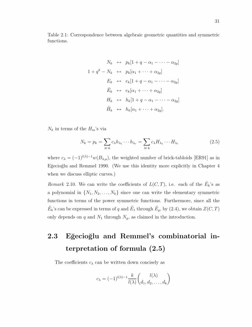
Table 2.1: Correspondence between algebraic geometric quantities and symmetricfunctions.

Nk ↔ pk[1 + q − α1 − · · · − α2g]

1 + qk −Nk ↔ pk[α1 + · · ·+ α2g]

Ek ↔ ek[1 + q − α1 − · · · − α2g]

Ek ↔ ek[α1 + · · ·+ α2g]

Hk ↔ hk[1 + q − α1 − · · · − α2g]

Hk ↔ hk[α1 + · · ·+ α2g].

Nk in terms of the Hm’s via

Nk = pk =∑

λ⊢k

cλhλ1 · · ·hλr =∑

λ⊢k

cλHλ1 · · ·Hλr (2.5)

where cλ = (−1)l(λ)−1w(Bλ,µ), the weighted number of brick-tabloids [ER91] as in

Egecioglu and Remmel 1990. (We use this identity more explicitly in Chapter 4

when we discuss elliptic curves.)

Remark 2.10. We can write the coefficients of L(C, T ), i.e. each of the Ek’s as

a polynomial in {N1, N2, . . . , Nk} since one can write the elementary symmetric

functions in terms of the power symmetric functions. Furthermore, since all the

Ek’s can be expressed in terms of q and E1 through Eg, by (2.4), we obtain Z(C, T )

only depends on q and N1 through Ng, as claimed in the introduction.

2.3 Egecioglu and Remmel’s combinatorial in-

terpretation of formula (2.5)

The coefficients cλ can be written down concisely as

cλ = (−1)l(λ)−1 k

l(λ)

(

l(λ)

d1, d2, . . . , dk

)

32

where l(λ) denotes the length of λ, which is a partition of k with type 1d12d2 · · · kdk .

We give one proof of this using Remmel’s interpretation using weighted brick-

tabloids, which can be derived by an equivalent combinatorial interpretation using

circular brick tabloids. (Note that the individual terms in these weighted counts

will differ, even though the weighted sums themselves are identical.) In Chapter 4

we will give an alternative proof simply using generating functions.

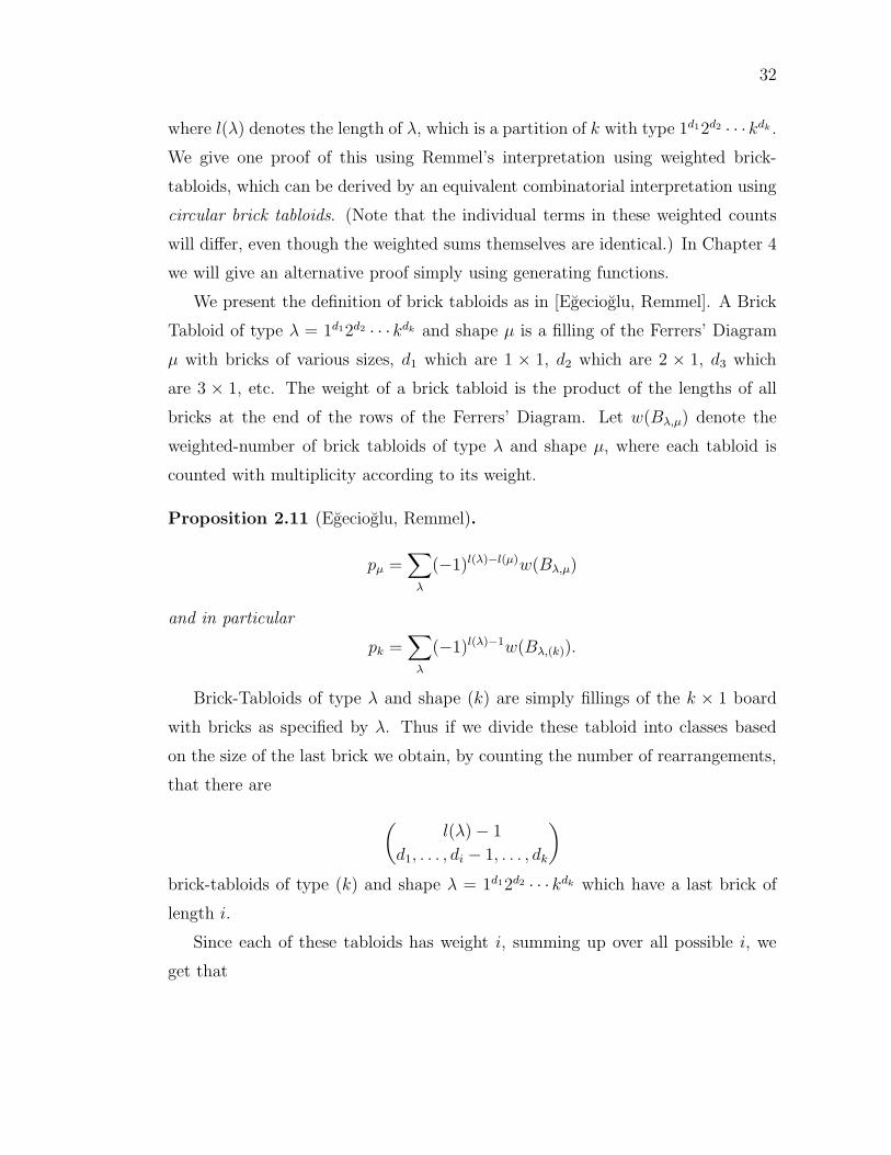
We present the definition of brick tabloids as in [Egecioglu, Remmel]. A Brick

Tabloid of type λ = 1d12d2 · · · kdk and shape µ is a filling of the Ferrers’ Diagram

µ with bricks of various sizes, d1 which are 1 × 1, d2 which are 2 × 1, d3 which

are 3 × 1, etc. The weight of a brick tabloid is the product of the lengths of all

bricks at the end of the rows of the Ferrers’ Diagram. Let w(Bλ,µ) denote the

weighted-number of brick tabloids of type λ and shape µ, where each tabloid is

counted with multiplicity according to its weight.

Proposition 2.11 (Egecioglu, Remmel).

pµ =∑

λ

(−1)l(λ)−l(µ)w(Bλ,µ)

and in particular

pk =∑

λ

(−1)l(λ)−1w(Bλ,(k)).

Brick-Tabloids of type λ and shape (k) are simply fillings of the k × 1 board

with bricks as specified by λ. Thus if we divide these tabloid into classes based

on the size of the last brick we obtain, by counting the number of rearrangements,

that there are

(

l(λ)− 1

d1, . . . , di − 1, . . . , dk

)

brick-tabloids of type (k) and shape λ = 1d12d2 · · · kdk which have a last brick of

length i.

Since each of these tabloids has weight i, summing up over all possible i, we

get that

33

w(Bλ,(k)) =k∑

i=0

i ·(

l(λ)− 1

d1, . . . , di − 1, . . . , dk

)

=

( k∑

i=0

idi

)

·(

l(λ)− 1

d1, . . . , di, . . . , dk

)

= k ·(

l(λ)− 1

d1, d2, . . . , dk

)

=k

l(λ)·(

l(λ)

d1, d2, . . . , dk

)

Note that the formula for cλ also appears elsewhere such as [Mac95]. Thus after

comparing signs, we obtain that cλ equals exactly the desired expression. Since

these formulas include terms with negative signs, we unfortunately cannot decom-

pose the set of points on curve C directly using these summands. Nonetheless, in

Section 2.5, we provide an interpretation of the cλ’s using inclusion-exclusion.

2.4 Alternative to plethysm

In many of the results involving identities of the Nk’s, Hk’s, and Ek’s we have

used the technique of plethystic substitution. In fact, lurking below many of these

proofs is the standard symmetric function identity that we have been using again

and again:∞∑

n=0

hnTn =

∏

k∈I

1

1− tkT= exp

(

∑

n=1

pnT n

n

)

where hn and pn are symmetric functions in the variables in I.So far we have just thought of Z(C, T ) as equal to this expression by letting hn

and pn be defined plethystically in the “alphabet” [1 + q − α1 − · · · − α2g]. While

this is internally consistent and shows why the ordinary generating function of the

Hk’s is equal to an exponential generating function of the Nk’s, it leaves less clear

why these expressions are both equal to

∏

p a prime or Frobenius Cycle

1

1− T deg p.

To see this more directly, we use cyclotomic polynomials. These polynomials will

be used again in Chapter 5 so this introduction provides a good warm-up.

34

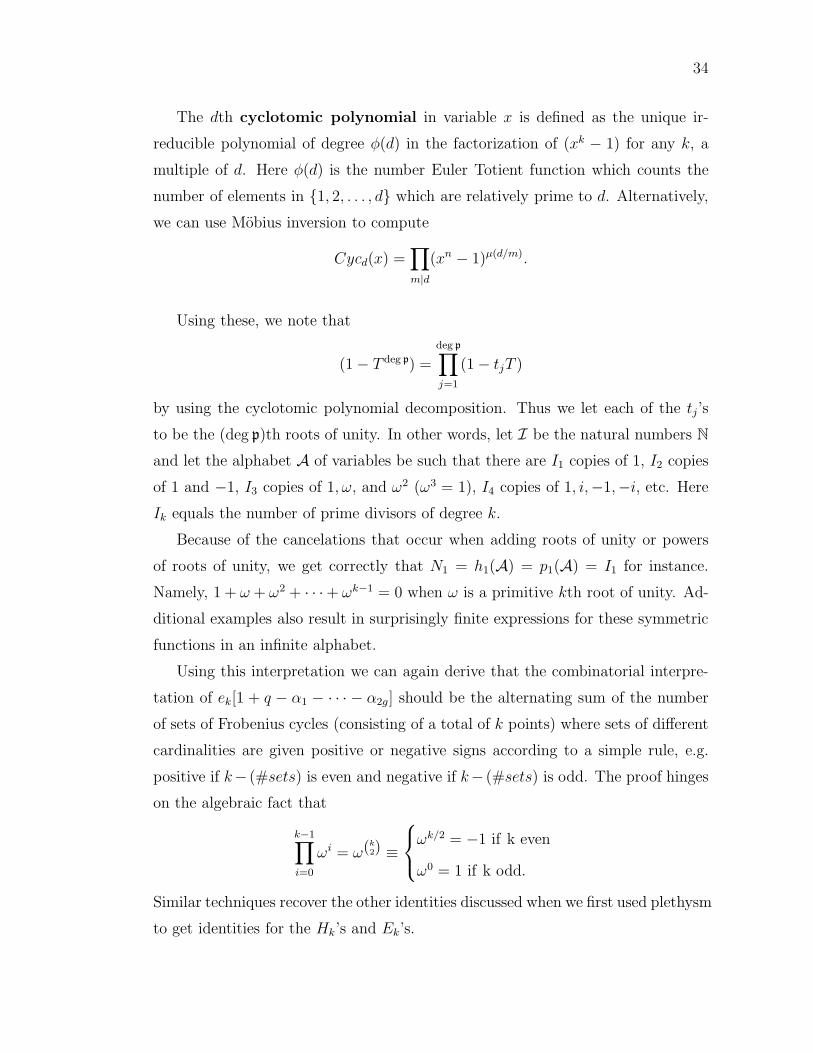
The dth cyclotomic polynomial in variable x is defined as the unique ir-

reducible polynomial of degree φ(d) in the factorization of (xk − 1) for any k, a

multiple of d. Here φ(d) is the number Euler Totient function which counts the

number of elements in {1, 2, . . . , d} which are relatively prime to d. Alternatively,

we can use Mobius inversion to compute

Cycd(x) =∏

m|d(xn − 1)µ(d/m).

Using these, we note that

(1− T deg p) =

deg p∏

j=1

(1− tjT )

by using the cyclotomic polynomial decomposition. Thus we let each of the tj’s

to be the (deg p)th roots of unity. In other words, let I be the natural numbers N

and let the alphabet A of variables be such that there are I1 copies of 1, I2 copies

of 1 and −1, I3 copies of 1, ω, and ω2 (ω3 = 1), I4 copies of 1, i,−1,−i, etc. Here

Ik equals the number of prime divisors of degree k.

Because of the cancelations that occur when adding roots of unity or powers

of roots of unity, we get correctly that N1 = h1(A) = p1(A) = I1 for instance.

Namely, 1 + ω + ω2 + · · ·+ ωk−1 = 0 when ω is a primitive kth root of unity. Ad-

ditional examples also result in surprisingly finite expressions for these symmetric

functions in an infinite alphabet.

Using this interpretation we can again derive that the combinatorial interpre-

tation of ek[1 + q − α1 − · · · − α2g] should be the alternating sum of the number

of sets of Frobenius cycles (consisting of a total of k points) where sets of different

cardinalities are given positive or negative signs according to a simple rule, e.g.

positive if k− (#sets) is even and negative if k− (#sets) is odd. The proof hinges

on the algebraic fact that

k−1∏

i=0

ωi = ω(k2) ≡

ωk/2 = −1 if k even

ω0 = 1 if k odd.

Similar techniques recover the other identities discussed when we first used plethysm

to get identities for the Hk’s and Ek’s.

35

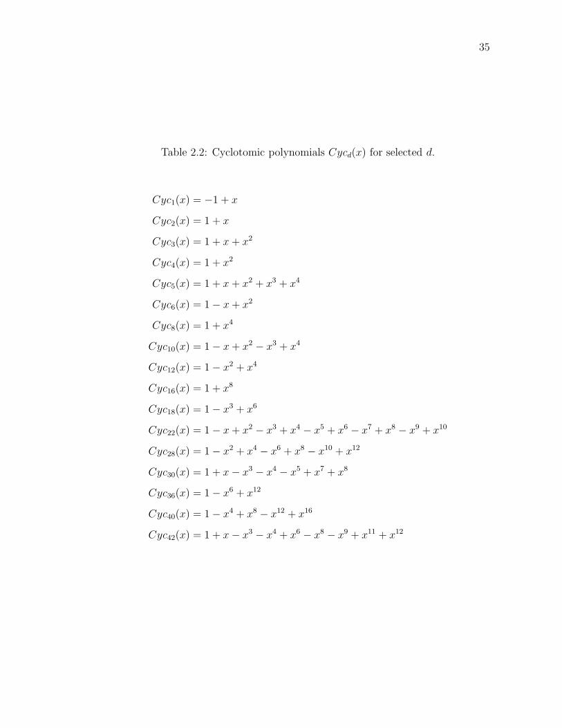
Table 2.2: Cyclotomic polynomials Cycd(x) for selected d.

Cyc1(x) = −1 + x

Cyc2(x) = 1 + x

Cyc3(x) = 1 + x+ x2

Cyc4(x) = 1 + x2

Cyc5(x) = 1 + x+ x2 + x3 + x4

Cyc6(x) = 1− x+ x2

Cyc8(x) = 1 + x4

Cyc10(x) = 1− x+ x2 − x3 + x4

Cyc12(x) = 1− x2 + x4

Cyc16(x) = 1 + x8

Cyc18(x) = 1− x3 + x6

Cyc22(x) = 1− x+ x2 − x3 + x4 − x5 + x6 − x7 + x8 − x9 + x10

Cyc28(x) = 1− x2 + x4 − x6 + x8 − x10 + x12

Cyc30(x) = 1 + x− x3 − x4 − x5 + x7 + x8

Cyc36(x) = 1− x6 + x12

Cyc40(x) = 1− x4 + x8 − x12 + x16

Cyc42(x) = 1 + x− x3 − x4 + x6 − x8 − x9 + x11 + x12

36

2.5 An inclusion-exclusion interpretation for (2.5)

We now describe the alternating formulas Nk =∑

λ⊢k cλHλ1Hλ2 · · ·Hλℓ(λ)by

counting the number of points via inclusion-exclusion on the number of divisors.

As a first example, consider the expression N2 = 2H2 − H1. We can understand

this equality by double-counting all positive divisors of degree two. Such divisors

come in two forms

D1 = P1 + P2, where P1 and P2 are degree one points,

D2 = Π = Q1 +Q2, where Q1 and Q2 are degree two points.

Let |D1| denote the number of divisors of type D1 and |D2| denote the number of

type D2. Consequently, 2H2 = 2|D1| + 2|D2| = 2|D1| + 2I2, where we recall I2

equals the number of prime divisors of degree 2 and 2I2 also equals the number

of points in C(Fq2) of degree 2. Thus we really want to count N2 = N1 + 2I2 but

2|D1| > N1, i.e. we have over-counted. To describe more fully how much we have

over-counted, we note a divisor of type D1 either looks like 2P1 or P1 + P2 with

P1 6= P2. There is a map between ordered pairs (P1, P2) of points in C(Fq) and

degree two divisors of type D1 by letting (P1, P2) 7→ P1 + P2. This map is 1-to-1

when P1 = P2 and 2-to-1 otherwise. Thus N21 , which counts the number of such

ordered pairs, equals N1 + |D1|, and so we subtract N21 , which is H2

1 , and obtain

the desired identity.

In fact we can repeat this same argument for higher cases and get in particular

H1 = I1

H2 = I2 +

((

I12

))

H3 = I3 + I2I1 +

((

I13

))

H4 = I4 + I3I1 +

((

I22

))

+ I2

((

I12

))

+

((

I14

))

, etc.

Here we are decomposing the number of positive divisors, of degree k, into types

of collections of multi-sets according to the possible partitions of k. Additionally,

Nk =∑

d|kd · Id.

37

Thus combining these relations, we get formulas for the Nk’s which illustrate the

above inclusion-exclusion pattern. We will give more explicit details for the elliptic

case in Chapter 4.

As a final comment, we note the resemblance between the above formulas for

Hk and Nk’s in terms of the Ik’s and a class of symmetric functions introduced by

Reutenauer, which are related to Witt vectors and the free Lie algebra. In [Reu95],

he discusses a family of symmetric functions defined by

∏

n≥1

1

1− qntn=∑

n≥0

hntn

which also implies that pi =∑

i=nk nqkn. In such a formula, the power symmetric

functions are called the ghost components of these qn’s.

3 Elliptic curves

The theory of elliptic curves is quite rich, arising in both the areas of complex

analysis and number theory. Such curves can be given a group structure using

the tangent-chord method or the divisor class group of algebraic geometry. This

property makes them not only geometric but also algebraic objects and allows

them to be used for cryptographic purposes. Because of their appearance in such

a varied number of subjects, we now will devote the rest of this thesis to this special

case. In this chapter we present the necessary background material and provide

details of some of the amazing facts that are true for the elliptic case. In particular,

we will discuss (1) the group structure on elliptic curves, (2) the theory of division

polynomials, and (3) how these can be used to prove a characteristic equation for

the Frobenius map. We follow sources such as [Gan], [Sil92], and [Was03] for the

material of this chapter.

3.1 Weierstraß form and group law

We recall from Chapter 1 that the Riemann-Roch Theorem tells us that a genus

g curve has L(D) of dimension given by

dimL(D)− dimL(K −D) = deg D + 1− g

where K is the canonical divisor, which has degree 2g − 2. In the case of genus

one, this gives an explicit description of such curves. Firstly, we have that K is a

divisor of degree 0 in the g = 1 case, and that for a divisor D0 of degree zero, that

L(D0) has dimension equal to the dimension of L(K −D0).

38

39

Proposition 3.1. For genus one curves, the canonical class contains the zero

divisor. Thus we set K = 0, up to class representative.

Proof. Recall by Lemma 1.15 that dimL(D) ≤ degD+1 and so in particular, if D0

has degree zero, L(D0) has dimension 0 or 1. Also during the course of the proof

of this lemma we noted that L(0) has dimension one since the constant functions

have no zeros or poles. Now assume there exists another D′ of degree zero such

that L(D′) also has nonzero dimension. Then there exists positive divisor D′′ and

rational function f such that D′ = D′′ + (f). However, since D′ is of degree zero,

so is D′′. However, we conclude D′′ = 0 since the only positive divisor of degree

zero is the zero divisor. Thus there is a unique class, the ones corresponding to

principal divisors, of degree zero divisors D with dim L(D) = 1. Finally, since

L(0) has the same dimension as L(K − 0) by Riemann-Roch, K must be in this

unique class, i.e. the same divisor class as 0.

Any degree zero divisor D0 besides those equivalent to 0 will have dim L(D0) = 0,

and dim L(0) = 1. Since the constant functions have divisor 0, we obtain for

degree zero D0

L(D0) =

{0} if D0 6≡ 0

k if D0 ≡ 0.

For divisors D of degree greater than 0, we have that deg (K − D) < 0 thus

dim L(D) = deg D. Using this dimension count, we can verify the following bases

for the below vector spaces:

L(P∞) = {1}

L(2P∞) = {1, x}

L(3P∞) = {1, x, y}

L(4P∞) = {1, x, y, x2}

L(5P∞) = {1, x, y, x2, xy}

L(6P∞) = {1, x, y, x2, xy, x3 = y2}

40

The upshot is that the quotient space L(6P∞)

/

L(5P∞) has dimension one but

spanning set {x3, y2}. Thus with respect to the genus one curve, we have the

relation

y2 − x3 = A1xy + A2x2 + A3y + A4x+ A6.

Theorem 3.2. Any genus 1 curve is in fact a hyperelliptic curve. We call such

curves elliptic curves. If the characteristic is not 2 or 3 the equation for the curve

can be written as

y2 = x3 + Ax+B

up to isomorphism. This is called the Weierstraß form of the curve. We call genus

1 curves elliptic curves.

Proof. We have done the heart of the proof above, we need only note that in

characteristic 6= 2, 3 we can algebraically manipulate, using techniques such as

completing the square, and choose x′ = α1x+β1 and y′ = α2y+β2x+γ2 such that

y′2

= x′3+ Ax′ +B.

Remark 3.3. Notice that the fact that L(P∞) is spanned by {1} also implies that

there is no nonconstant function which has a pole at exactly one point on an elliptic

curve. Thus, there are N1 degree one positive divisors and they are all inequivalent.

Another amazing fact about the special case of elliptic curves is the existence

of a group law. Thereby, the curve is not only a geometric object, but also an

algebraic object.

Definition 3.4. If C, over an arbitrary field k, is defined by equation

y2 = x3 + Ax+B

and P1 = (x1, y1), P2 = (x2, y2), then

P1 ⊕ P2 = P3 = (x3, y3)

where

41

1) If x1 6= x2 then

x3 = m2 − x1 − x2 and y3 = m(x1 − x3)− y1 with m =y2 − y1

x2 − x1

.

2) If x1 = x2 but (y1 6= y2, or y1 = 0 = y2) then P3 = P∞.

3) If P1 = P2 and y1 6= 0, then

x3 = m2 − 2x1 and y3 = m(x1 − x3)− y1 with m =3x2

1 + A

2y1.

4) The point at infinity, P∞, acts as the identity element in this addition.

Lemma 3.5. Definition 3.4 yields an associative abelian group on the set of points

on C, including P∞.

We note that since the group law is defined explicitly, the associativity can

be directly verified, though one needs to be careful to include all of the cases.

However, since we have previously proven the Riemann-Roch Theorem, we instead

give a shorter proof using this result. Before proceeding, we need the following

lemma.

As we saw above, there exists a divisor class of degree one for all points on the

curve. In fact we have the stronger result

Lemma 3.6. Any degree m divisor is equivalent to a divisor of the form

D = P +mP∞

where P is a point on the curve, possibly P∞.

Proof. By Rieman-Roch the divisor of a line, which is a rational function, is a

degree zero divisor. Bezout’s Theorem [Har77] tells us that the number of points

on the intersection of a degree three rational function, y2 = x3 + Ax + B, and a

degree one rational function, ay + bx + c = 0 is 3 · 1 = 3 counting multiplicities.

Thus the divisor of a line on a curve is equal to

P +Q+R − 3P∞

42

with P,Q,R, P∞ not necessarily distinct. Thus given divisor

D = D+ −D−

where bothD+ andD− are both positive divisors we can use various lines to reduce

D+ and D− separately.

We have that for every P , Q (including Q = P ) on the curve, their sum is

equivalent to −R + 3P∞. Secondly, we have that the line x = a contains both

the points (a, b) and (a,−b) (and P∞ as the third point). This includes the case

where line x = a is tangent, multiplicity two, to the point (a, 0). Thus the divisor

P(a,b) + P(a,−b) − 2P∞ ≡ 0 and we have that −R + 3P∞ ≡ R + P∞ where R is

the conjugate point (Rx,−Ry). By repeated application, we are left with a single

point plus a multiple of the point at infinity.

Proof of Lemma 3.5. Thus we can define the group law, in fact it is inherited from

the divisor class group, as

P ⊕Q = R ⇐⇒ (P − P∞) + (Q− P∞) ≡ (R − P∞).

Associativity and commutativity thereby come for free. We only need to check this

geometric description using lines is equivalent to the above algebraic description.

By the fact that the three points P1 = (x1, y1), P2 = (x2, y2), and −P3 = (x3,−y3)

lie on the same line, we have by similar triangles that

(−y3)− y1

x3 − x1=y2 − y1

x2 − x1.

Rearranging this equality gives us the formula for y3. To get the expression for x3

takes a little more work.

We first notice that for all (x, y) on the elliptic curve, y = m(x−x1)+y1 where

m is the slope y2−y1

x2−x1. Since we have the equality y2 = x2 +Ax+B, we also obtain

that

0 = x3 −m2x2 + . . . .

The three roots of this equation are exactly the three x-coordinates for the points

in the intersection of line L through P1 and P2 and elliptic curve C. Consequently,

43

since the coefficient of the quadratic term is the negative of the sum of the roots,

m2 = x1 + x2 + x3

and after rearrangement, we have our expression for x3. The case of doubling a

point using tangent lines is analogous.

3.2 Rational function representations of

morphisms

We will define an endomorphism α : E → E of an elliptic curve as a ho-

momorphism, with respect to the group law, that can be represented as a pair of

rational functions gα and hα. In other words, α fixes P∞ and

α(x, y) =

(

gα(x, y), hα(x, y)

)

and (gα+β, hα+β) = (gα, hα)⊕ (gβ, hβ)

since

(α + β)(P ) = α(P )⊕ β(P ).

We will closely follow Section 2.8 of [Was03] in this subsection as we discuss further

properties of endomorphisms.

Since α is a group homomorphism, it maps the identity P∞ to itself. Borrowing

from geometric language, an endomorphism is also sometimes referred to as an

isogeny since it has such a fixed point. We will refer to α as the zero map if it

sends every point of E to P∞ and nontrivial otherwise.

We first note the following algebraic geometric fact concerning endomorphisms.

Theorem 3.7. Let E be defined over Fq (in fact any algebraically closed field).

Then an endomorphism α is either surjective or the zero map.

Proof. See [Gan], [Har77] for a proof, or [Was03, Thm 2.21] for a more elementary

approach.

Lemma 3.8. For elliptic curves, and more generally hyperelliptic curves, we can

rationalize rational functions in k(C) so that they are of the form p1(x)+p2(x)yp3(x)

where

the pi’s are polynomials.

44

Proof. If g is a rational function in k(C) of the form P (x,y)Q(x,y)

, we have the relation

y2 = f0(x), e.g. f0(x) = x3 + Ax+B in the elliptic case. Thus we can rewrite

P (x, y)

Q(x, y)=A(x) + yB(x)

C(x) + yD(x)=

(A(x) + yB(x))(C(x)− yD(x))

C(x)2 − y2D(x)

and the denominator can again be simplified so it is univariate in x.

In fact in the elliptic case, we can describe these rational functions even more

precisely.

Lemma 3.9. If α(x, y) =

(

gα(x, y), hα(x, y)

)

is an endomorphism of an elliptic

curve, then

gα is univariate in terms of x and hα = y hα(x).

where hα(x) is a univariate rational function.

Proof. We obtain these last expressions by using the group law and the fact that

α is a homomorphism to obtain

α(x,−y) = α(⊖(x, y)) = ⊖α(x, y).

Consequently, the x-coordinate of α(x, y), i.e gα(x, y) satisfies gα(x, y) = gα(x,−y)and analogously, hα(x, y) = −hα(x,−y). Thus gα has no y-coordinate and hα has

no x-coordinate.

Notational convention: if we wish to write these rational functions as polynomials

we will write

gα as nα(x)/dα(x) and hα as y nα(x)/dα(x)

such that both pairs nα, dα and nα, dα have no common factors.

Note that since these are rational functions, as opposed to polynomials, there

will exist choices of x ∈ Fq such that the denominators are zero. A priori it might

appear that it would be possible for one of dα(x0), dα(x0) to be zero and not the

other but we will shortly find that we can consistently define α

(

(x0, y0)

)

= P∞

in this case by the following lemma.

45

Lemma 3.10. For any x0 ∈ Fq, either both dα(x0) and dα(x0) 6= 0 or both dα(x0)

and dα(x0) = 0. Thus, in the former case we have α

(

(x0, y0)

)

= (a, b) ∈ Fq2 ∩E,

and the latter we have α

(

(x0, y0)

)

= P∞.

Proof. First we note that the coordinates of α

(

(x, y)

)

, i.e. (gα, hα) = (gα, y hα)

satisfy the defining equation

h2α = g3

α + A gα +B.

Thus

h2α = y2hα

2=

(x3 + Ax+B) nα(x)2

dα(x)2=

˜nα(x)

dα(x)3

for polynomial ˜nα(x) with no common factor with dα(x). More precisely, ˜nα(x) =

n3α(x)+A nα(x) dα(x)2+B dα(x)3 and nα(x) has no factors in common with dα(x).

If dα(x0) = 0 then the denominator of the square of hα is also zero hence

dα(x0) = 0. If, on the other hand, dα(x0) = 0 then we might have that x0 is a root

of both x3 +A x+B and dα(x)2, however the first expression has no multiple roots

since E(Fq) was assumed to be a nonsingular curve, and the second has roots with

multiplicities at least two. Thus the denominator will still be zero in this case,

hence dα(x0) = 0 as well. By the contrapositive, we have that one of these is

nonzero if and only if the other is nonzero too.

Remark 3.11. We will see this relationship between gα and hα again when we study

division polynomials in Section 3.3, namely, that there exists a polynomial Ψα(x)

such that Ψα(x)2 = dα(x) and Ψα(x)3 = dα(x).

With this last lemma in mind, we note that the first coordinate alone deter-

mines whether or not α(P ) = P∞, and in fact only the denominator matters, which

motivates the following definition. We define the degree of nontrivial endomor-

phism α to be

deg(α) = Max{deg nα(x), deg dα(x)}.

The degree of the zero map is set to be 0. This quantity degree is important for

several different reasons.

46

1. The deg(α) serves as an upper bound for the size of the Ker α with equality

in many cases. We will shortly make this rigorous.

2. A map α between curves E1 and E2 induces an contravariant injection α∗

between funciton fields k(E2) and k(E1). In this context, the degree of map

α is equal to the degree of the field extension k(E1)/k(α(E1)).

3. We will see in Section 3.4 that the n-torsion subgroup (when gcd(n, q) = 1)

of an elliptic curve is isomorphic to a lattice and thus endomorphisms can

also be represented as 2−by−2 matrices. In this context, the deg(α) is equal

to the determinant modulo n.

4. Using this 2−by−2 matrix interpretation, or otherwise, we obtain that degree

gives rise to a quadratic form on the space of endomorphisms; more precisely

deg(rα+ sβ) = r2 deg(α) + s2 deg(β) + rs

(

deg(α+ β)− deg(α)− deg(β)

)

.

We now proceed to make precise the relationship between degree and the size

of Ker α. We begin by calling a nontrivial endomorphism α separable if the

derivative of rational function gα(x) is not identically zero. Recall that gα is the

rational function corresponding to the x-coordinate of α((x, y)).

Remark 3.12. One can also formulate the notion of separability using algebraic

language, namely that α is separable if and only if it induces a separable extension

on function fields. In other words,

α : E1 → E2

is separable if and only if

α∗ : k(E2) : k(E1)

induces

k(E1)/α∗(k(E2)) a separable field extension.

While this definition has its advantages, to be able to utilize it properly, we would

have to discuss notions such as ramification degree that would take us away from

our goal. One can find such an approach in [Sil92].

47

We see from the next Lemma, that one need not check separability at the ratio-

nal function level, but that it suffices to check it for the corresponding polynomials.

Lemma 3.13. Using our notation, gα(x) = nα(x)/dα(x) for univariate polynomi-

als nα, dα with no common factors, we have that α is separable if and only if at

least one of ddxnα(x) = n′

α(x) or ddxdα(x) = d′α(x) is not identically zero.

Proof. ddx

(

nα(x)dα(x)

)

= 0 if and only if the numerator, using the quotient rule for

derivation,

dα(x)n′α(x)− nα(x)d′α(x) = 0.

Since dα(x) is assumed to be 6= 0, if we further assume that d′α(x) 6= 0, we get that

nα(x)

dα(x)=n′

α(x)

d′α(x)

where both n′α(x) and d′α(x) have degrees smaller than nα(x) and dα(x), respec-

tively. Since nα(x)/dα(x) had been assumed to be in lowest terms we get a con-

tradiction. Thus we must have d′α(x) is identically zero, and hence n′α(x) = 0 also

from the above equality.

Now that we have reduced the notion of separability to considering polynomials,

we can use the following observation to determine whether or not α is separable.

Lemma 3.14. If the characteristic of our field is zero, then any nonconstant poly-

nomial will have a nonzero derivative. If the characteristic is p, then any polyno-

mial with zero derivative is of the form P (xp), or equivalently P (x)p, for polynomial

P .

Proof. The derivative of a polynomial anxn+· · ·+a1x+a0 is nanx

n−1+· · ·+2a2x+a1

which is the zero polynomial if and only if all the coefficients kak ≡ 0 mod p. Thus

the only terms with nonzero coefficients must be those with exponents a multiple

of p. Since (yp + zp) = (y + z)p in characteristic p, we have the result.

Proposition 3.15. If α 6= 0 is a separable endomorphism of elliptic curve E over

Fq, or another algebraically closed field, then

deg(α) = # Ker(α).

48

If α 6= 0 is not separable, then

deg(α) > # Ker(α).

Proof. See [Was03, Ch. 2].

3.3 Division polynomials and the multiplication

by n map

This section is based on notes from [Cas91], [Lan78], [Was03, pg.77], and

[Was03, Sec. 9.5]. To better understand the group structure of elliptic curves,

we define a sequence of polynomials in Z[x, y, A,B] via the following initial condi-

tions and recurrence equations:

ψ0 = 0

ψ1 = 1

ψ2 = 2y

ψ3 = 3x4 + 6Ax2 + 12Bx− A2

ψ4 = 4y(x6 + 5Ax4 + 20Bx3 − 5A2x2 − 4ABx− 8B2 − A3)

· · ·

ψ2m+1 = ψm+2ψ3m − ψm−1ψ

3m+1 for m ≥ 2

ψ2m = (ψm

2y) · (ψm+2ψ

2m−1 − ψm−2ψ

2m+1) for m ≥ 2

The polynomial ψn is known as the nth division polynomial. These polynomials

turn out to have the remarkable property that all of the finite n-torsion points

(x0, y0), i.e. elements of E[n] \ {P∞}, satisfy ψ2n(x0, y0) = 0. Here E is shorthand

for E(Fq) and E[n] signifies those points in E in the kernel of the multiplication

by n map sending P 7→ P ⊕ P ⊕ · · · ⊕ P . In fact we can describe this property

more precisely.

Proposition 3.16. For the ψn as defined above, we have the alternative definition

that for n ∈ Z, then ψn(x, y) is defined as the unique rational function such that

49

ψn(x, y)2 = n2 ·∏

Pi=(ai,bi)∈E[n]\{P∞}

(x− ai)

and ψn(x, y) has leading term +n.

Additionally, we can define the multiple of a point, r ·(x, y), as a pair of rational

functions in terms of x and y using the ψn’s. In particular, we have the following:

Proposition 3.17. Let P = (x, y) be a point on the elliptic curve y2 = x3+Ax+B

over some field of characteristic 6= 2. Then for any positive integer n, nP =

P ⊕ P ⊕ P ⊕ · · · ⊕ P is given by

nP =

(

φn(x)

ψ2n(x)

,ωn(x, y)

ψ3n(x, y)

)

=

(

x− ψn−1ψn+1

ψ2n(x)

,ψ2n(x, y)

2ψ4n(x)

)

.

−nP =

(

φn(x)

ψ2n(x)

, − ωn(x, y)

ψ3n(x, y)

)

=

(

x− ψn−1ψn+1

ψ2n(x)

, − ψ2n(x, y)

2ψ4n(x)

)

where the polynomials φn and ωn are defined as

φm = xψ2m − ψm+1ψm−1

ωm =ψm+2ψ

2m−1 − ψm−2ψ

2m+1

4y.

Proof. For the proofs of Propositions 3.16 and 3.17, see [Lan78] or [Was03, Ch.

9].

Note that by Proposition 3.16 or via the equivalence relation y2 ≡ x3 +Ax+B

and the recurrence relations for ψ2m and ψ2m+1, we can inductively prove that

ψ2n,

ψ2n

y, ψ2n+1, and φn are all functions in terms of x.

As a corollary, the x-coordinate of nP is a rational function strictly in terms of x,

and the y-coordinate has the form y ·Θ(x).

We can summarize these results as follows: ψ2 is a function in x alone and has

degree n2 − 1, which equals the number of finite n-torsion points. The degree of

ψ2 is easily verified via the above recurrence relations. Furthermore, if n is odd

and (x0, y0) ∈ E \ {P∞}, then

ψn(x0) = 0 if and only if (x0, y0) ∈ E[n].

50

If n is even, E is defined by equation y2 = (x− α1)(x− α2)(x− α3) over Fq, and

(x0, y0) ∈ E \ {P∞, (α1, 0), (α2, 0), (α3, 0)}, then

ψn

y(x0) = 0 if and only if (x0, y0) ∈ E[n].

Corollary 3.18. The degree of the endomorphism of multiplication by n has degree

n2.

Proof. This is simply because the maximum of the degrees of φn(x) and ψ2n(x),

which in fact only depend on x, is n2.

Corollary 3.19. If gcd(n, p) = 1 then α = [n] is a separable endomorphism, thus

the #Ker(α) = deg(α) = n2.

Proof. See [Sil92] or [Was03] for example, for the proof that [n] is separable when

gcd(n, p) = 1.

In particular, when this morphism is separable, it has no multiple roots. Thus

since the degree of the denominator is n2 − 1, we have n2 − 1 values of α ∈ Fp we

can plug in to obtain a zero denominator, i.e. an x-coordinate of ∞.

Hence, if we let P = P∞ or (α, β) where α a zero of φ2n(x), we obtain nP = P∞.

There are n2 such possibilities, thus n2 elements in the kernel of this separable

morphism, and the multiplication by n map has degree n2.

Note in the case gcd(n, p) > 1 the multiplication map is not separable. The

degree is still n2, but the size of the kernel is smaller since there will be multiple

roots.

Corollary 3.20. If gcd(n, p) = 1 then the group E[n] ∼= Z/nZ× Z/nZ.

Proof. Based on [Gan]. We have just proven that the group E[n] satisfies #E[n] =

n2 in this case. By the Fundamental Theorem of Finite Abelian Groups, we have

that

E[n] ∼= (Z/n1Z)d1 × · · · × (Z/nkZ)dk

such that n1|n2| . . . |nk and n2 = nd11 · · ·ndk

k .

Assume that n1 < n. Then E[n] contains a cyclic subgroup of order n1 hence

elements of order n1. Thus E[n] would have E[n1], the [n1]-torsion points as a

51

subgroup. E[n1] inherits its structure from E[n] and since n1 was assumed to be the

smallest we have that E[n1] ∼= (Z/n1Z)d1 which implies that d1 = 2. Furthermore,

every generator of a cyclic subgroup of E[n] would also be a generator for a cyclic

subgroup of E[n1] since n1 divides all thier orders. Thus the cyclic decomposition

of E[n1] tells us that there at most two cyclic subgroup of E[n], and we have that

E[n] ∼= (Z/n1Z)× (Z/n′1Z), and since n1n

′1 = n2, we have n1 = n′

1 = n.

Corollary 3.21. The abelian group E(Fqk), for any elliptic curve E over finite

field Fqk , can be decomposed as a product of at most two cyclic groups, i.e. of form

E(Fqk) ∼= ZN1 × ZN2

where N1|N2.

Proof. Since |E(Fqk)| is finite, there exists an N such that E(Fqk) ⊂ E(Fq)[N ].

Thus E(Fqk) is a subgroup of E(Fq)[N ] ∼= ZN × ZN . Assume that E(Fq)[N ] is

generated by α and β, both of degree N . Then any subgroup of E(Fqk) will have

at most two generators. Lastly, if N1 6 |N2 then N1 = ac, N2 = bc with gcd(a, b) = 1

such that gcd(a, c) = 1 without loss of generality, and a 6= 1. Thus letting N ′1 = c,

N ′2 = abc, we obtain ZN1 × ZN2

∼= ZN ′1× ZN ′

2with N ′

1|N ′2.

Remark 3.22. Division polynomials ψn(x, y) are also an example of an elliptic

divisibility sequence (EDS) [War48], which means

1) ψn|ψm iff n|m.

2) The recurrence

ψn+mψn−m = ψ2mψn−1ψn+1 − ψm−1ψm+1ψ

2n (3.1)

is satisfied. (Note that we proved recurrence (3.1) in the course of proving Propo-

sition 3.16.)

3) Alternatively, we could let m = 2 and shift indices to see that the ψn’s (or

for that matter, any EDS) satisfy

ψnψn−4 = (ψ22)ψn−1ψn−3 + (−ψ1ψ3)ψ

2n−2

This is a special case of the Somos-4 sequence [Pro] which in general looks like:

snsn−4 = αsn−1sn−3 + βs2n−2.

52

4) A proper EDS {sn} satisfies s0 = 0, s1 = 1, s2|s4. Note that the division

polynomials ψn(x, y) satisfy this property.

There has been recent literature regarding this pattern, in particular for specific

curves, the x-coordinates of the rational points form a Somos sequence. We invite

the reader to read [VDPS06], [Pro], or [Swa] for more details. This sequence is a

manifestation of the interplay between elliptic curves and combinatorics. We will

discuss other connections of a different flavor starting in the next chapter.

3.4 Further properties of the Frobenius map

We now describe the remarkable properties of the Frobenius map in the special

case of elliptic curves. One important property of the Frobenius map is its com-

patibility with the group law on elliptic curves over Fq. In particular, we have the

following:

Proposition 3.23. If we let π signify the Frobenius map, then we have the relation

π(P ⊕Q) = π(P )⊕ π(Q) (3.2)

for points P,Q ∈ C(Fq).

Proof. This follows by explicit verification using the algebraic formulas for the

group law, taking care to include the various cases.

Because of the reason that equation (3.2) resembles the distributive law, we

sometimes refer to “acting by” the Frobenius map as multiplication by the Frobe-

nius map. The Frobenius map allows to rephrase our main goal, namely calculating

the order of E(Fqk), as the calculation of #Ker(1− πk). We have that for a ∈ Fq,

πk(a) = a if and only if a ∈ Fqk .

Since π

(

(x, y)

)

= (xq, yq), we easily see that deg(π) = q. However, ddxxq =

qxq−1 ≡ 0 hence the Frobenius map is inseparable. Nonetheless we obtain

Lemma 3.24. The endomorphism

rπ + s

53

(r, s ∈ Z) is separable if and only if gcd(s, q) = 1. In particular, 1− π is separable

and

Nk = #Ker(1− πk) = deg(1− πk).

Proof. See [Was03, Ch. 2].

Recall from Corollary 3.20 that E(Fq)[n] ∼= Z/nZ × Z/nZ if gcd(n, q) = 1.

Since π is a morphism which acts on E(Fq)[n] (since π ◦ [n] = [n] ◦ π implies

that nP = P∞ ⇔ n ◦ π(P ) = P∞), we have that π’s action on E(Fq)[n] can be

represented by a 2× 2 matrix with coefficients in Z/nZ.

As a consequence π satisfies a quadratic characteristic equation

π2 − tnπ + dn = 0

on E(Fq)[n], thus π satisfies

π2 − tnπ + dn ≡ 0 (mod n).

Since we get such a quadratic characteristic equation for an infinite set of n satis-

fying gcd(n, q) = 1, we find a unique t, d ∈ Z such that

π2 − tπ + d = 0

on all points of E(Fq) with order relatively prime to q. There are an infinite number

of such points.

Proposition 3.25. For all points P ∈ E(Fq), we have the identity π2− tπ+d = 0

where t = 1 + q −N1 and d = q.

Proof. See [Was03] for the details on why t and d are specifically 1 + q − N1 and

q respectively. Once this is verified for all n such that gcd(n, p) = 1, we note

that the expression π2 − tπ + d is also a morphism which can be represented by

a pair of rational functions (using the definition of the Frobenius map, division

polynomials, composition, and the group law). Thus there can only be a finite

number of elements in the kernel, unless it is the zero map. Thus we obtain

π2 − tπ + d = 0

on all of E(Fq).

54

In fact, by considering the inverse limit of the sequence {E(Fq)[ℓk]}, where

each term is isomorphic to Z/ℓkZ × Z/ℓkZ, we recover a construction of the Tate

Module, a two dimensional space on which the Frobenius endomorphism acts. See

[Sil92] for more on the Tate Module. One of the surprising and important results of

etale cohomology is that the choice of prime ℓ does not matter for this calculation,

as long as ℓ 6= p. In this respect, the value t is the trace of the Frobenius map, and

d is the determinant of the Frobenius map under this 2-dimensional action.

4 Combinatorial aspects of ellip-

tic curves

Recall that when E is an elliptic curve, Z(E, T ) can be expressed as

1− (α1 + α2)T + α1α2T2

(1− T )(1− qT )

and in particular we have

Nk = 1 + qk − αk1 − αk

2 = pk[1 + q − α1 − α2].

Plugging in k = 1 the relation α1 + α2 = 1 + q −N1 and we note that α1α2 = q is

a special case of the zeta function’s functional equation we saw in Chapter 1.

Hence we can rewrite the zeta function Z(E, T ) totally in terms of q and N1

and as a consequence, all the Nk’s are actually dependent on these two quantities.

This data gives rise to the following observation of Adriano Garsia.

Table 4.1: Nk’s as polynomials for small k.

N2 = (2 + 2q)N1 −N21

N3 = (3 + 3q + 3q2)N1 − (3 + 3q)N21 +N3

1

N4 = (4 + 4q + 4q2 + 4q3)N1 − (6 + 8q + 6q2)N21 + (4 + 4q)N3

1 −N41

N5 = (5 + 5q + 5q2 + 5q3 + 5q4)N1 − (10 + 15q + 15q2 + 10q3)N21

+ (10 + 15q + 10q2)N31 − (5 + 5q)N4

1 +N51

55

56

Theorem 4.1.

Nk =

k∑

i=1

(−1)i−1Pi,k(q)Ni1

where the Pi,k’s are polynomials with positive integer coefficients.

This theorem is proved by Garsia using induction and the fact that the sequence

of Nk’s satisfy a simple recurrence. For the details, see [GM, Chap. 7]. This result

motivates the following combinatorial question:

Question 4.2. What are the objects that the family of polynomials, {Pi,k}, enu-

merate?

We will answer this questions in due course, in multiples ways, thus providing

an alternate proof of Theorem 4.1.

4.1 First answer to Question 4.2

In this section we provide two different combinatorial interpretations for the

coefficients of the Pk’s.

4.1.1 The Lucas numbers and a (q, t)-analogue

Definition 4.3. Let S(n)1 be the circular shift of set S ⊆ {1, 2, . . . , n} modulo

n, i.e. element x ∈ S(n)1 if and only if x − 1 ( mod n ) ∈ S. We define the

(q, t)−Lucas numbers to be the sequence of polynomials in variables q and t

Ln(q, t) =∑

S⊆{1,2,...,n} : S∩S(n)1 =∅

q# even elements in S t⌊n2⌋−#S. (4.1)

Note that this sum is over subsets S with no two numbers circularly consecutive.

These polynomials are a generalization of the sequence of Lucas numbers Ln

which have the initial conditions L1 = 1, L2 = 3 (or L0 = 2 and L1 = 1) and

satisfy the Fibonacci recurrence Ln = Ln−1 + Ln−2. The first few Lucas numbers

are

1, 3, 4, 7, 11, 18, 29, 47, 76, 123, . . .

57

As described in numerous sources, e.g. [BY06], Ln is equal to the number of ways

to color an n−beaded necklace black and white so that no two black beads are

consecutive. You can also think of this as choosing a subset of {1, 2, . . . , n} with

no consecutive elements, nor the pair 1, n. (We call this circularly consecutive.)

Thus letting q and t both equal one, we get by definition that Ln(1, 1, ) = Ln.

We will prove the following theorem, which relates our newly defined

(q, t)−Lucas numbers to the polynomials of interest, namely the Nk’s.

Theorem 4.4.

1 + qk −Nk = L2k(q,−N1) (4.2)

for all k ≥ 1.

To prove this result it suffices to prove that both sides are equal for k ∈ {1, 2},and that both sides satisfy the same three-term recurrence relation. Since

L2(q, t) = 1 + q + t and

L4(q, t) = 1 + q2 + (2q + 2)t+ t2

we have proven that the initial conditions agree. Note that the sets of (4.1) yielding

the terms of these sums are respectively

{1}, {2}, { } and {1, 3}, {2, 4}, {1}, {2}, {3}, {4}, { }.

It remains to prove that both sides of (4.2) satisfy the recursion

Gk+1 = (1 + q −N1)Gk − qGk−1

for k ≥ 1.

Proposition 4.5. For the (q, t)−Lucas Numbers Lk(q, t) defined as above,

L2k+2(q, t) = (1 + q + t)L2k(q, t)− qL2k−2(q, t). (4.3)

Proof. To prove this we actually define an auxiliary set of polynomials, {L2k}, such

that

L2k(q, t) = tkL2k(q, t−1).

58

Thus recurrence (4.3) for the L2k’s translates into

L2k+2(q, t) = (1 + t+ qt)L2k(q, t)− qt2L2k−2(q, t)

for the L2k’s. The L2k’s happen to have a nice combinatorial interpretation also,

namely

L2k(q, t) =∑

S⊆{1,2,...,2k} : S∩S(2k)1 =∅

q# even elements in S t#S.

Recall our slightly different description which considers these as the generating

function of 2-colored, labeled necklaces. We will find this terminology slightly

easier to work with. We can think of the beads labeled 1 through 2k + 2 to be

constructed from a pair of necklaces; one of length 2k with beads labeled 1 through

2k, and one of length 2 with beads labeled 2k + 1 and 2k + 2.

Almost all possible necklaces of length 2k + 2 can be decomposed in such a

way since the coloring requirements of the 2k+2 necklace are more stringent than

those of the pairs. However not all necklaces can be decomposed this way, nor can

all pairs be pulled apart and reformed as a (2k + 2)-necklace.

In Figure 4.1 the first necklace is decomposable but the second one is not since

black beads 1 and 4 would be adjacent, thus violating the rule. It is clear enough

that the number of pairs is L2(q, t)L2k(q, t) = (1+ t+ qt)L2k(q, t). To get the third

term of the recurrence, i.e. qt2L2k−2, we must define linear analogues, Fn(q, t)’s, of

the previous generating function. Just as the Ln(1, 1)’s were Lucas numbers, the

Fn(1, 1)’s will be Fibonacci numbers.

Definition 4.6. The (twisted) (q, t)−Fibonacci polynomials, denoted as Fn(q, t),

are defined as

Fk(q, t) =∑

S⊆{1,2,...,k−1} : S∩(S(k−1)1 −{1})=∅

q# even elements in S t#S.

The summands here are subsets of {1, 2, . . . , k − 1} such that no two elements

are linearly consecutive, i.e. we now allow a subset with both the first and last

elements. An alternate description of the objects involved are as (linear) chains

of k − 1 beads which are black or white with no two consecutive black beads.

59

For example, if k = 2:

Decomposable

1 2

3

45

6

→

6

5 4

3

21

Not Decomposable

1 2

3

45

6

6→

6

5 4

3

21

Figure 4.1: Illustrating proof of Proposition 4.5.

With these new polynomials at our disposal, we can calculate the third term of

the recurrence, which is the difference between the number of pairs that cannot be

recombined and the number of necklaces that cannot be decomposed.

Lemma 4.7. The number of pairs that cannot be recombined into a longer necklace

is 2qt2F2k−2(q, t).

Proof. We have two cases: either both 1 and 2k + 2 are black, or both 2k and

2k+1 are black. These contribute a factor of qt2, and imply that beads 2, 2k, and

2k + 1 are white, or that 1, 2k − 1, and 2k + 2 are white, respectively. In either

case, we are left counting chains of length 2k− 3, which have no consecutive black

beads. In one case we start at an odd-labeled bead and go to an evenly labeled

one, and the other case is the reverse, thus summing over all possibilities yields

the same generating function in both cases.

Lemma 4.8. The number of (2k + 2)-necklaces that cannot be decomposed into a

2-necklace and a 2k-necklace is qt2F2k−3(q, t).

60

Proof. The only ones that cannot be decomposed are those which have beads 1

and 2k both black. Since such a necklace would have no consecutive black beads,

this implies that beads 2, 2k − 1, 2k + 1, and 2k + 2 are all white. Thus we are

reduced to looking at chains of length 2k− 4, starting at an odd, 3, which have no

consecutive black beads.

Lemma 4.9. The difference of the quantity referred to in Lemma 4.8 from the

quantity in Lemma 4.7 is exactly qt2L2k−2(q, t).

Proof. It suffices to prove the relation

qt2L2k−2(q, t) = 2qt2F2k−2(q, t)− qt2F2k−3(q, t)

which is equivalent to

qt2L2k−2(q, t) = qt2F2k−2(q, t) + q2t3F2k−4(q, t) (4.4)

since

F2k−2(q, t) = qtF2k−4(q, t) + F2k−3(q, t). (4.5)

Note that identity (4.5) simply comes from the fact that the (2k − 2)nd bead can

be black or white. Finally we prove (4.4) by dividing by qt2, and then breaking it

into the cases where bead 1 is white or black. If bead 1 is white, we remove that

bead and cut the necklace accordingly. If bead 1 is black, then beads 2 and 2k+2

must be white, and we remove all three of the beads.

With this lemma proven, the recursion for the L2k’s, hence the L2k’s follows

immediately.

Proposition 4.10. For an elliptic curve C with Nk points over Fqk we have that

1 + qk+1 −Nk+1 = (1 + q −N1)(1 + qk −Nk)− q(1 + qk−1 −Nk−1).

Proof. Recalling that for an elliptic curve C we have the identity

Nk = 1 + qk − αk1 − αk

2 ,

61

we can rewrite the statement of this proposition as

αk+11 + αk+1

2 = (α1 + α2)(αk1 + αk

2)− q(αk−11 + αk−1

2 ). (4.6)

Noting that q = α1α2 we obtain this proposition after expanding out algebraically

the right-hand-side of (4.6).

With the proof of Propositions 4.5 and 4.10, we have proven Theorem 4.4.

4.1.2 (q, t)−Wheel numbers

Given that we found the Lucas numbers are related to the polynomial formulas

Nk(q,N1), a natural question concerns how alternative interpretations of the Lucas

numbers can help us better understand Nk. As noted in [BY06], [Mye71], and [Slo,

Seq. A004146], the sequence {L2n−2} counts the number of spanning trees in the

wheel graph Wn; a graph which consists of n+1 vertices, n of which lie on a circle

and one vertex in the center, a hub, which is connected to all the other vertices.

Definition 4.11. An undirected graph G = (V,E) is defined by vertex set V and

an edge set E consisting of pairs (vi, vj) where vi and vj ∈ V . A subgraph of G is

defined as G′ = (V ′, E ′) where V ′ is a subset of V and E ′ is a subset of E consisting

of edges using only vertices of V . A spanning tree of graph G is a connected

subgraph G′ (there exists a path from any vertex to another using the edges of G′)

which contains no cycles, i.e. there is exactly one path from one vertex to another.

We note that a spanning tree T of Wn consists of spokes and a collection of

disconnected arcs on the rim. Further, since there are no cycles and T is connected,

each spoke will intersect exactly one arc. (Since it will turn out to be convenient

in the subsequent considerations, we make the – somewhat counter-intuitive –

convention that an isolated vertex is considered to be an arc of length 1, and more

generally, an arc consisting of k vertices is considered as an arc of length k.) We

imagine the circle being oriented clockwise, and imagine the tail of each arc being

the vertex which is the sink for that arc. In the case of an isolated vertex, the lone

vertex is the tail of that arc. Since the spoke intersects each arc exactly once, if

an arc has length k, meaning that it contains k vertices, there will be k choices

62

of where the spoke and the arc meet. We define the q−weight of an arc to be

q number of edges between the spoke and the tail, abbreviating this exponent as spoke− taildistance. We define the q−weight of the tree to be the product of the q−weights

for all arcs on the rim of the tree. This combinatorial interpretation motivates the

following definition.

Definition 4.12.

Wn(q, t) =∑

T a spanning tree of Wn

qsum of spoke−tail distance in T t# spokes of T .

Here the exponent of t counts the number of edges emanating from the central

vertex, and the exponent of q is as above.

q2t3

dist = 1

dist = 1

dist = 0

q3t3

dist = 0

dist = 1

dist = 2

Figure 4.2: Illustrating definition of Wn(q, t).

This definition actually provides exactly the generating function that we de-

sired.

Theorem 4.13.

Nk = −Wk(q,−N1)

for all k ≥ 1.

Notice that this yields an exact interpretation of the Pi,k polynomials as follows:

Pi,k(q) =∑

T a spanning tree of Wn with exactly i spokes

qsum of spoke−tail distance in T .

We will prove this theorem in two different ways. The first method will utilize

Theorem 4.4 and an analogue of the bijection given in [BY06] which relates perfect

63

and imperfect matchings of the circle of length 2k and spanning trees of Wk.

Our second proof will use the observation that we can categorize the spanning

trees based on the sizes of the various connected arcs on the rims. Since this

categorization will correspond to partitions, this method will exploit formulas for

decomposing power symmetric function pk into a linear combination of hλ’s, as

described in Chapter 2.

4.1.3 First proof of Theorem 4.13: Bijective

There is a simple bijection between subsets (of size at most n−1) of {1, 2, . . . , 2n}with no two elements circularly consecutive and spanning trees of the wheel graph

Wn. We will use this bijection to give our first proof of Theorem 4.13. The bijection

is as follows:

Given a subset S of the set {1, 2, . . . , 2n−1, 2n} with no circularly consecutive

elements, we define the corresponding spanning tree TS of Wn (with the correct q

and t weight) in the following way:

1) We will use the convention that the vertices of the graph Wn are labeled so

that the vertices on the rim are w1 through wn, and the central vertex is w0.

2) We will exclude the two subsets which consist of all the odds or all the evens

from this bijection. Thus we will only be looking at subsets which contain n − 1

or fewer elements.

3) For 1 ≤ i ≤ n, an edge exists from w0 to wi if and only if neither 2i− 2 nor

2i− 1 (element 0 is identified with element 2n) is contained in S.

4) For 1 ≤ i ≤ n, an edge exists from wi to wi+1 (wn+1 is identified with w1) if

and only if element 2i− 1 or element 2i is contained in S.

Proposition 4.14. Given this construction, TS is in fact a spanning tree of Wn

and further, tree TS has the same q−weights and t−weights as set S.

Proof. Suppose that set S contains k elements. From our above restriction, we have

that 0 ≤ k ≤ n−1. Since S is a k-subset of a 2n element set with no circularly con-

secutive elements, there will be (n−k) pairs {2i−2, 2i−1} with neither element in

set S, and k pairs {2i− 1, 2i} with one element in set S. Consequently, subgraph

64

Or Elt 6

Elt 5

Elt 4 Or

Elt 3

Elt 2

Elt 1 Or

Not 5

Not 4

Not 3

Not 2

And Not 6

Not 1

And

And

{ }

←→

{

3

}

←→{

2, 5

}

←→

Figure 4.3: Illustrating bijection of Theorem 4.13.

TS will consist of exactly (n−k)+k = n edges. Since n = (# vertices of Wn)−1, to

prove TS is a spanning tree, it suffices to show that each vertex of Wn is included.

For every oddly-labeled element of {1, 2, . . . , 2n}, i.e. 2i−1 for 1 ≤ i ≤ n, we have

the following rubric:

1) If (2i− 1) ∈ S then the subgraph TS contains the edge from wi to wi+1.

2) If (2i − 1) 6∈ S and additionally (2i − 2) 6∈ S, then TS contains the spoke

from w0 to wi.

3) If (2i−1) 6∈ S and additionally (2i−2) ∈ S, then TS contains the edge from

wi−1 to wi.

Since one of these three cases will happen for all 1 ≤ i ≤ n, vertex wi is incident

to an edge in TS. Also, the central vertex, w0, has to be included since by our

restriction, 0 ≤ k ≤ n−1, there are (n−k) ≥ 1 pairs {2i−2, 2i−1} which contain

no elements of S.

The number of spokes in TS is (n−k) which agrees with the t−weight of a set S

with k elements. Finally, we prove that the q-weight is preserved, by induction on

the number of elements in the set S. If set S has no elements, the q−weight should

65

be q0, and spanning tree TS will consist of n spokes which also has q−weight q0.

Now given a k element subset S (0 ≤ k ≤ n − 2), it is only possible to adjoin

an odd number if there is a sequence of three consecutive numbers starting with

an even, i.e. {2i − 2, 2i − 1, 2i}, which is disjoint from S. Such a sequence of S

corresponds to a segment of TS where a spoke and tail of an arc intersect. (Note

this includes the case of vertex wi being an isolated vertex.)

In this case, subset S ′ = S ∪ {2i − 1} corresponds to TS′ , which is equivalent

to spanning tree TS except that one of the spokes w0 to wi has been deleted and

replaced with an edge from wi to wi+1. The arc corresponding to the spoke from

wi will now be connected to the next arc, clockwise. Thus the distance between

the spoke and the tail of this arc will not have changed, hence the q−weight of TS′

will be the same as the q−weight of TS.

Alternatively, it is only possible to adjoin an even number to S if there is

a sequence {2i − 1, 2i, 2i + 1} which is disjoint from S. Such a sequence of S

corresponds to a segment of TS where a spoke meets the end of an arc. (Note this

includes the case of vertex wi being an isolated vertex.)

Here, subset S ′′ = S ∪{2i} corresponds to TS′′ , which is equivalent to spanning

tree TS except that one of the spokes w0 to wi+1 has been deleted and replaced

with an edge from wi to wi+1. The arc corresponding to the spoke from wi+1 will

now be connected to the previous arc, clockwise. Thus the cumulative change to

the total distance between spokes and the tails of arcs will be an increase of one,

hence the q−weight of TS′′ will be q1 times the q−weight of TS.

Since any subset S can be built up this way from the empty set, our proof is

complete via this induction.

Since the two sets we excluded, of size k had (q, t)−weights q0t0 and qkt0

respectively, we have proven Theorem 4.13.

66

4.1.4 Second proof of Theorem 4.13: Via generating func-

tion identities

For our second proof of Theorem 4.13, we consider writing the zeta function as

an ordinary generating function instead, i.e.

Z(C, T ) = 1 +∑

k≥1

HkTk. (4.7)

In such a form, the Hk’s are positive integers which enumerate the number of

positive C(Fq)-divisors of degree k, as noted in several places, such as [Mor91].

Proposition 4.15.

Nk =∑

λ⊢k

(−1)l(λ)−1 k

l(λ)

(

l(λ)

d1, d2, . . . dm

) l(λ)∏

i=1

Hλi. (4.8)

Proof. Comparing formulas (1.2) and (4.7) for Z(C, T ) and taking logarithms, we

obtain

Nk

k= log Z(C, T )

∣

∣

∣

∣

T k

= log

(

1 +∑

n≥1

HnT n

)∣

∣

∣

∣

T k

=∑

m≥1

(−1)m−1

(

∑kn=1 HnT n

)m

m

∣

∣

∣

∣

T k

.

To obtain the coefficient of T k in(

H1T +H2T2 + · · ·+HkT

k

)m

, (4.9)

we first select a partition of k with length ℓ(λ) = m. In other words, λ is a vector of

positive integers satisfying λ1 ≥ λ2 ≥ · · · ≥ λm. Each occurrence of λi = j in this

partition corresponds to choosing summand HjTj in the ith term in product (4.9).

Secondly, since the order of these terms does not matter, we include multinomial

coefficients. Finally, multiplying through by k yields formula (4.8) for Nk.

As we saw in Chapter 2, these identities between Nk and Hk are equivalent to

those between pk and hk and thus the theory of symmetric functions also supplies

a proof of Proposition 4.15 specializing to the genus one case.

67

We now specialize to the case of g = 1. Here we can write Hk in terms of N1

and q. We expand the series

Z(E, T ) =1− (1 + q −N1)T + qT 2

(1− T )(1− qT )= 1 +

N1T

(1− T )(1− qT )(4.10)

with respect to T , and obtain H0 = 1 and Hk = N1(1 + q + q2 + · · · + qk−1) for

k ≥ 1. Plugging these into formula (4.8), we get polynomial formulas for Nk in

terms of q and N1

Nk =∑

λ⊢k

(−1)l(λ)−1 k

l(λ)

(

l(λ)

d1, d2, . . . dk

)( l(λ)∏

i=1

(1 + q + q2 + · · ·+ qλi−1)

)

Nl(λ)1 .

Consequently, Theorem 4.13 is true if and only if we can replace N1 with −tand then multiply by (−1) and get a true expression for Wk, the (q, t)-weighted

number of spanning trees on the wheel graph Wk. We thus provide the following

combinatorial argument for the required formula.

Proposition 4.16.

Wk =∑

λ⊢k

k

l(λ)

(

l(λ)

d1, d2, . . . dk

)( l(λ)∏

i=1

(1 + q + q2 + · · ·+ qλi−1)

)

tl(λ). (4.11)

Proof. We will construct a spanning tree of Wk from the following choices: First

we choose a partition λ = 1d12d2 · · · kdm of k. We let this dictate how many arcs of

each length occur, i.e. we have d1 isolated vertices, d2 arcs of length 2, etc. Note

that this choice also dictates the number of spokes, which is equal to the number

of arcs, i.e. the length of the partition.

Second, we pick an arrangement of the l(λ) arcs on the circle. After picking

one arc to start with, without loss of generality since we are on a circle, we have

1

l(λ)

(

l(λ)

d1, d2, . . . dm

)

choices for such an arrangement. Third, we pick which vertex wi of the rim to start

with. There are k such choices. Fourth, we pick where the l(λ) spokes actually

intersect the arcs. There will be |arc| choices for each arc, and the q−weight of this

sum will be (1 + q+ q2 + · · ·+ q|arc|) for each arc. Summing up all the possibilities

yields (4.11) as desired.

Thus we have given a second proof of Theorem 4.13.

68

4.2 More on bivariate Fibonacci polynomials via

duality

In this section we explore further properties of various sequences of coefficients

arising from the zeta function of a curve, and also more properties regarding bivari-

ate Fibonacci polynomials. Our tools for such investigations will be two different

manifestations of duality.

4.2.1 Duality between the symmetric functions hk and ek

Recall that in Section 4.1.1, we defined Fk(q, t), i.e. the twisted (q, t)-Fibonacci

polynomials. Here we define Fk(q, t), an alternative bivariate analogue of the

Fibonacci numbers. The definition of Fk(q, t) is identical to that of Fk(q, t) except

for the weighting of parameter t.

Definition 4.17. We define the (q, t)-Fibonacci polynomials to be the sequence

of polynomials in variables q and t given by

Fk(q, t) =∑

S⊆{1,2,...,k−1} : S∩(S(k−1)1 −{1})=∅

q# even elements in S t⌈k2⌉−#S.

From this definition we obtain the following formulas for the Ek’s in the elliptic

case.

Theorem 4.18. If C is a genus one curve, and the Ek’s are as above, then for

n ≥ 1, E−n = 0, E0 = 1, and

En = (−1)nF2n−1(q,−N1)

where Ek and Fk(q, t) are as defined above.

Before proving Theorem 4.18 we develop two key propositions.

Proposition 4.19. F2n+1(q, t) = (1 + q + t)F2n−1(q, t)− qF2n−3(q, t) for n ≥ 2.

69

Table 4.2: Ek, i.e. F2k−1(q, t)’s for small k for the special case of an elliptic curve.

E1 = N1

E2 = −(1 + q)N1 +N21

E3 = (1 + q + q2)N1 − (2 + 2q)N21 +N3

1

E4 = −(1 + q + q2 + q3)N1 + (3 + 4q + 3q2)N21 − (3 + 3q)N3

1 +N41

E5 = (1 + q + q2 + q3 + q4)N1 − (4 + 6q + 6q2 + 4q3)N21

+ (6 + 9q + 6q2)N31 − (4 + 4q)N4

1 +N51

Proof. This follows the similar logic as the proof of Proposition 4.5 except we can

use a more direct method. (One can use the t-weighting of the twisted (q, t)-

Fibonacci polynomials instead to see this recursion more clearly, but we will omit

this detour.) The polynomial F2n+1 is a (q, t)-enumeration of the number of chains

of 2n beads, with each bead either black or white, and no two consecutive beads

both black. Similarly (1+q+t)F2n−1 enumerates the concatenation of such a chain

of length 2n− 2 with a chain of length 2. One can recover a legal chain of length

2n this way except in the case where the (2n−2)nd and (2n−1)st beads are both

black. Such cases are enumerated by qF2n−3 and this completes the proof.

Proposition 4.20. (−1)n+1En+1 = (1+q−N1)(−1)nEn−q(−1)n−1En−1 for n ≥ 2.

Proof. We use the plethystic identity

ek[A +B] =

k∑

i=0

ei[A]ek−i[B]

for any alphabets A and B. Setting A = α1 + α2 and B = 1 + q − α1 − α2, we

derive

en+1[1 + q] = en+1[1 + q − α1 − α2] + (α1 + α2)en[1 + q − α1 − α2]

+ (α1α2)en−1[1 + q − α1 − α2]

= En+1 + (1 + q −N1)En + qEn−1.

Since en+1[1 + q] = 0 for n ≥ 2, we obtain the proposition as desired.

70

This result also follows directly from the generating function for the En’s which

is given by∑

n≥0

(−1)nEnTn =

(1− T )(1− qT )

1− (1 + q −N1)T + qT 2.

The denominator of this series, also known as the series’ characteristic polynomial,

yields the desired linear recurrence for the coefficients of T n+1, whenever n + 1

exceeds the degree of the numerator.

With these two propositions verified, we can also now prove Theorem 4.18.

Proof of Theorem 4.18. It is clear that E1 = −F1(q,−N1), E2 = F3(q,−N1), and

E3 = −F5(q,−N1). Propositions 4.19 and 4.20 show that both satisfy the same

recurrence relations. Thus we have verified that

En = (−1)nF2n−1(q,−N1).

Plethysm is a powerful tool and we utilize it below to obtain results of a similar

flavor to Proposition 4.20.

Lemma 4.21. Letting Ek be defined as ek[1 + q − α1 − α2] where α1 and α2 are

roots of T 2 − (1 + q −N1)T + q, we obtain

hk[α1 + α2] = (−1)kEk+1/N1.

Proof. We have for n ≥ 2 that

N1En = En+1 + (1 + q)En + qEn−1

since (−1)n+1En+1 = (1 + q − N1)(−1)nEn − q(−1)n−1En−1 by Proposition 4.20.

However by

ek[A− B] =k∑

i=0

ei[A](−1)k−ihk−i[B],

we get

En+1 = (−1)n+1

(

hn+1[α1 + α2]− (1 + q)hn[α1 + α2] + qhn−1[α1 + α2]

)

71

using A = 1+ q and B = α1 +α2. After verifying initial conditions and comparing

with

(−1)n+1En+1 = (−1)n+1En+2/N1 − (−1)n(1 + q)En+1/N1 + (−1)n−1qEn/N1

we get

hn+1[α1 + α2] = (−1)n+1En+2/N1

by induction.

With this result in mind, we obtain a table of symmetric function ek and hk in

terms of various alphabets.

Table 4.3: Plethysm of ek, hk for elliptic curves.

poly. \ alphabet 1 + q − α1 − α2 1 + q α1 + α2

ek Ek e1 = 1 + q, e2 = q e1 = 1 + q −N1, e2 = q

hk Hk 1 + q + · · ·+ qk (−1)kEk+1/N1

(We had earlier referred to Ek versus Ek and Hk versus Hk for plethysm in the

alphabets 1 + q− α1 − α2 and α1 + α2, respectively.) Notice that the formulas for

ek[1+ q] and hk[1+ q] are precisely the N1 = 0 cases of ek[α1 +α2] and hk[α1 +α2].

This should come at no surprise since 1 and q are the two roots of T 2−(1+q)T +q.

The plethystic equalities

hk[A+B] =

k∑

i=0

hi[A]hk−i[B]

and

hk[A−B] =k∑

i=0

hi[A](−1)k−iek−i[B],

as well as the expressions for ek[A+B] and ek[A−B] used above, give rise to even

more identities for different choices of A and B. We have focused on the ones that

we have since they appeared most useful.

The above Hk–Ek (i.e. hk–ek) duality generalizes to the case of higher genus

curves. However, considering the genus one case further, we take advantage of

72

the simplicity of this particular generating function. Recall, as in (4.10), that by

rewriting equation (1.14) we obtain

Z(E, T ) = 1 +N1T

(1− qT )(1− T )

when E is an elliptic curve. As an application, we obtain an exponential generating

function for the weighted number of spanning trees of the wheel graph,

W (q,N1, T ) = exp

(

∑

k≥1

Wk(q,N1)T k

k

)

.

Using Wk = −Nk|N1→−N1, and the fact this is an exponential, we obtain

W (q,N1, T ) =1

1− N1T(1−qT )(1−T )

=(1− qT )(1− T )

1− (1 + q +N1)T + qT 2.

Also, rewriting W (q, t, T )as an ordinary generating function, we get

W (q, t, T ) =∑

k≥0

Ek

∣

∣

∣

∣

N1→−N1

(−T )k = 1 +∑

k≥1

F2k−1(q, t)Tk.

Table 4.4: Plethystic dictionary for elliptic curves and spanning trees.

Elliptic Curves Spanning Trees

Generating Function1−(1+q−N1)T+qT 2

(1−qT )(1−T )(1−qT )(1−T )

1−(1+q+N1)T+qT 2

1− (1 + q ∓N1)T + qT 2 = (1− α1T )(1− α2T ) (1− β1T )(1− β2T )

Nk (resp. Wk ) pk[1 + q − α1 − α2] pk[−1− q + β1 + β2]

Hk = N1(1 + q + · · ·+ qk−1) hk[1 + q − α1 − α2] (−1)k−1ek[−1− q + β1 + β2]

(−1)kEk = F2k−1(q,∓N1) (−1)kek[1 + q − α1 − α2] hk[−1− q + β1 + β2]

4.2.2 Duality between Lucas and Fibonacci numbers

In addition to the above discussion of how Hk and Ek are dual, this dic-

tionary also highlights a comparison between elliptic curve–spanning tree dual-

ity and duality between Lucas numbers and Fibonacci numbers. As an appli-

cation, we obtain a formula for Ek, i.e. F2k−1(q, t), in terms of the polyno-

mial expansion for the L2k(q, t)’s. If we recall our definition of Pi,k’s such that

73

Nk =∑k

i=1(−1)i+1Pi,k(q)Ni1, or equivalently L2k(q, t) = 1 + qk +

∑ki=1 Pi,k(q)t

i,

then we have

Proposition 4.22.

Ek =

k∑

i=1

(−1)k+i · ik

Pi,k(q)Ni1.

To verify Proposition 4.22 we need the following combinatorial lemma, which

describes a connection between the sets enumerated by Lucas numbers and those

sets enumerated by Fibonacci numbers.

Lemma 4.23. For 1 ≤ i ≤ k and 0 ≤ j ≤ i, we have the number, which we denote

as ci,j, of subsets S1 of {1, 2, . . . , 2k} with k− i− j odd elements, j even elements,

and no two elements circularly consecutive equals

k

i·#(

subsets S2 of {1, 2, . . . , 2k−2} with k−i−j odd elments, j even elements,

and no two elements consecutive

)

.

This notation might seem non-intuitive, but we use these indices so that the

total number of elements is k − i and the number of even elements is j. Thus the

number of subsets S1 (resp. S2) directly describes the coefficient of qjti in L2k(q, t)

(resp. F2k−1(q, t)).

Proof. To prove this result we note that there is a bijection between the number

of subsets of the first kind that do not contain 2k−1 or 2k and those of the second

kind. Thus it suffices to show that the number of sets S1 which do contain element

2k− 1 or 2k is precisely fraction k−ik

of all sets S1 satisfying the above hypotheses.

Circularly shifting every element of set S1 by an even amount r, i.e. ℓ 7→ℓ + r − 1 (mod 2k) + 1, does not affect the number of odd elments and even

elements. Furthermore, out of the k possible even shifts, (k − i) of the sets, i.e.

the cardinality of set S1, will contain 2k − 1 or 2k. This follows since for a given

element ℓ there is exactly one shift which makes it 2k − 1 (or 2k) if ℓ is odd (or

even), respectively. Since elements cannot be consecutive, there is no shift that

sends two different elements to both 2k−1 and 2k simultaneously and thus we get

the full (k − i) possible shifts.

74

With this lemma proven, we can now show Proposition 4.22.

Proof of Proposition 4.22. We recall that

Wk(q,N1) = L2k − 1− qk =k∑

i=1

Pi,k(q)Ni1 =

k∑

i=1

k∑

j=0

ci,jNi1q

j and

F2k−1(q,−N1) = (−1)kEk.

Furthermore, we just showed via Lemma 4.23 that

F2k−1(q,N1) =k∑

i=1

k∑

j=0

i

kci,jN

i1q

j =k∑

i=1

i

kPi,k(q)N

i1.

Using Theorem 4.18 completes the proof.

Remark 4.24. Alternatively, one can arrive at this result by directly manipulating

the generating function. Namely, using the identities as above, we observe that1

Z(E,T )=∑

n≥0(−1)nEnTn, and so we have

∑

n≥1

(−1)nEnT n =1

Z(E, T )− 1 =

1

1 + N1T(1−qT )(1−T )

− 1 =∑

n≥1

(−1)n

(

N1T

(1− qT )(1− T )

)n

= −N1∂

∂N1

∑

n≥1

(−1)n−1

n

(

N1T

(1 − qT )(1− T )

)n

= −N1∂

∂N1

(

log

(

1 +N1T

(1− qT )(1− T )

))

= −N1∂

∂N1log

(

Z(E, T )

)

,

which equals −N1∂

∂N1

(

∑

k≥1Nk

kT k

)

. Rewriting the Nk’s using the polynomial

formulas of Theorem 4.1, we have

∑

n≥1

(−1)nEnTn = −N1

∂

∂N1

(

∑

k≥1

1

k

k∑

i=1

(−1)i−1Pi,k(q)Ni1T

k

)

=∑

k≥1

k∑

i=1

i

k(−1)iPi,k(q)N

i1T

k.

Comparing the coefficients of T k on both sides completes the proof.

Lemma 4.23 also provides us a way to obtain expressions for Pi,k(q), and in

particular Ek and Nk, in terms of binomial coefficients.

75

Proposition 4.25. For k ≥ 1 and 1 ≤ i ≤ k, we have

Pi,k(q) =

i∑

j=0

k

i

(

k − 1− ji− 1

)(

i+ j − 1

j

)

qj.

Proof. See [Zel07, Theorem 2.2] or [MP07, Theorem 3] which show by algebraic

and combinatorial arguments, respectively, that the number of ways to choose a

subset S ⊂ {1, 2, . . . , 2n} such that S contains q odd elements, r even elements,

and no consecutive elements is(

n− rq

)(

n− qr

)

.

Letting n = k − 1, q = k − i− j and r = j, we obtain

i

kPi,k(q) = F2k−1(q,N1)

∣

∣

∣

∣

N i1

=i∑

j=0

(

k − 1− ji− 1

)(

i+ j − 1

j

)

qj.

Corollary 4.26.

Nk(q,N1) =k∑

i=1

i∑

j=0

(−1)i+1 · ki

(

k − 1− ji− 1

)(

i+ j − 1

j

)

N i1 q

j.

and

Ek =k∑

i=1

i∑

j=0

(−1)k+i

(

k − 1− ji− 1

)(

i+ j − 1

j

)

N i1 q

j .

Remark 4.27. From the proof in Section 4.1.4, we have that

Wk(q,N1) =∑

λ⊢k

k

l(λ)

(

l(λ)

d1, d2, . . . dr

)( l(λ)∏

i=1

(1 + q + q2 + · · ·+ qλi−1)

)

Nl(λ)1

=

k∑

i=1

k

i

(

∑

λ⊢k

l(λ)=i

(

i

d1, d2, . . . dr

) i∏

j=1

(1 + q + q2 + · · ·+ qλj−1)

)

N i1

which implies also that

Pi,k(q) =k

i

∑

λ⊢k

l(λ)=i

(

i

d1, d2, . . . dr

) i∏

j=1

(1 + q + q2 + · · ·+ qλj−1).

Comparing the coefficients of this identity with the coefficients in Proposition 4.25

seems to give a combinatorial identity that seems interesting in its own right.

76

We have just seen how Nk is equal to pk[1 + q − α1 − α2] plethystically and

how this sequence relates to the sequences Hk = hk[1 + q − α1 − α2] and Ek =

ek[1 + q − α1 − α2] via symmetric function theory. We close this section with a

matrix determinant for pk[α1 + α2] = 1 + qk −Nk from [GM, Chapter 7].

Proposition 4.28. 1 + qk −Nk equals

det

1 + q −N1 −1 0 0 0 0

−2q 1 + q −N1 −1 0 0 0

0 −q 1 + q −N1 −1 0 0...

......

. . .. . . 0

0 0 0 · · · 1 + q −N1 −1

0 0 0 · · · −q 1 + q −N1

where this matrix is k-by-k. We denote this matrix as M ′k.

Proof. By the Newton Identities [Sta99], the power symmetric functions pk can

be rewritten in terms of the elementary symmetric functions ek. In particular,

1 + qk −Nk = 1 + qk − pk[1 + q − α1 − α2] = pk[α1 + α2] can be rewritten as

det

e1[α1 + α2] −1 0 0 0

−2e2[α1 + α2] e1[α1 + α2] −1 0 0...

.... . .

. . . 0

(−1)k(k − 1)ek−1[α1 + α2] (−1)k−1ek−2[α1 + α2] · · · e1[α1 + α2] −1

(−1)k+1kek[α1 + α2] (−1)kek−1[α1 + α2] · · · −e2[α1 + α2] e1[α1 + α2]

.

Finally, since e1[α1 + α2] = α1 + α2 = 1 + q − N1, e2[α1 + α2] = α1α2 = q, and

ek[α1 + α2] = 0 for all k ≥ 2, we have proven the proposition.

4.3 Case-Study on N2 = (2 + 2q)N1 −N21

In this section, we investigate a method for understanding an elliptic curve E

over a finite field Fp2k (p prime) by understanding the elliptic curve restricted to

Fpk as well as a second curve over Fpk which is known as the (quadratic) twist of

E(Fpk). For convenience, we will take q to be pk and assume p ≥ 5, i.e. not char

77

2 or 3. This will allow us to write elliptic curve E as defined by the equation

y2 = x3 + ax+ b

where a, b ∈ Fq. We will let f(x) denote x3 + ax + b, E represent the set of

all points with coordinates in the algebraic closure Fq, and let E(Fqn) denote the

subset E∩F2qn . One of the beauties of elliptic curves is that the sets E and E(Fqn)

have additional structure, namely they are abelian groups whose addition we will

denote as ⊕. By abuse of notation, E and E(Fqn) will signify these groups. We

need to define one more operation, and then we will be able to state the main

theorem of this section.

Definition 4.29. If E(Fq) is an elliptic curve with coefficients in Fq and Λ ∈ Fq,

let Et(Λ)(Fq) represent the quadratic twist (with respect to Λ) of E(Fq) defined as

follows: if E has equation y2 = f(x), then Et(Λ) has equation

y2 = Λf(x).

Proposition 4.30. Et(Λ)(Fq) is isomorphic to the curve with equation

y′ 2 = x′ 3 + aΛ−2x′ + bΛ−3.

Proof. If y2 = Λ(x3 + ax+ b), then letting y = Λ2y′, x = Λx′, we obtain

y′ 2Λ4 = x′ 3Λ4 + ax′Λ2 + bΛ

Dividing through by Λ4, this becomes

y′ 2 = x′ 3 + aΛ−2x′ + bΛ−3.

Proposition 4.31. If we have two elliptic curves over Fq in the simplified Weier-

straß form, i.e.

y2 = x3 + Ax+B (4.12)

y2 = x3 + A′x+B′ (4.13)

then curve (4.12) ∼= curve (4.13) if and only if there exists ω ∈ Fq \ {0} such that

A′ = ω4A and B′ = ω6B.

78

Proof. Two curves are isomorphic if we can change coordinates so that

x′ = αx+ β

y′ = γx+ δy + ǫ

but the only way we can do this so that y′ 2 and x′ 3 have the same coefficients

while y′, x′y′ and x′ 2 have coefficients of zero is if β, γ, ǫ all equal 0, and α2 = δ3,

which implies there exists ω = δα

such that ω−2 = δ, ω−3 = α. Thus there

exists ω ∈ Fq \ {0} such that the transformation x′ = ω−2x, y′ = ω−3y yields an

isomorphic curve. After plugging in these into

y2 = x3 + Ax+B

and multiplying through by ω6, we get the desired equation

y2 = x3 + ω4Ax+ ω6B.

Proposition 4.32. If Λ is a square in Fq, then Et(Λ)(Fq) ∼= E(Fq).

Proof. If Λ = λ2 for λ ∈ Fq, then we let y = λy′ and obtain via this change of

coordinates that y′ 2 = f(x) whenever (x, y) satisfy y2 = Λf(x).

Proposition 4.33. If Λ is a non-square in Fq, then Et(Λ)(Fq) 6∼= E(Fq), but

Et(Λ)(Fq) ∼= Et(Λ′)(Fq) for any other Λ′ ∈ Fq which is a non-square.

Proof. The curve Et(Λ)(Fq) is isomorphic to a curve with the equation

y′ 2 = x′ 3 + aΛ−2x′ + bΛ−3.

This is the simplified Weierstraß form, and thus Et(Λ)(Fq) is isomorphic to E(Fq)

if only if there exists ω ∈ Fq \ {0} such that Λ−2 = ω4,Λ−3 = ω6, which implies

that Λ is a square over Fq. ⇒⇐

In light of these results, we will drop the superscript (Λ) from our notation,

and let Et(Fq) represent Et(Λ)(Fq) where Λ is any non-square of Fq. We now come

to the main result of this section.

79

Theorem 4.34. If E is a non-singular elliptic curve with coefficients in Fq, and

Et(Fq) is its quadratic twist over Fq, as defined above, then

|E(Fq2)| = |E(Fq)| · |Et(Fq)|. (4.14)

Furthermore, there is an explicit bijection between sets E(Fq2) and E(Fq)×Et(Fq),

as well as a group isomorphism in many cases.

We will prove this theorem in three steps. First we demonstrate the validity

of equality (4.14) algebraically. Secondly, we provide an alternative proof of this

identity by illustrating an explicit bijection between these two sets. We then

discuss the problem of constructing a natural bijection and give a simple criterion

for determining when we in fact have a group isomorphism. We begin algebraically.

4.3.1 Algebraic proof

Lemma 4.35. |Et(Fq)| = 2q + 2− |E(Fq)|.

Proof. This result appears several places in the literature, for example [Hus04] We

provide a proof of this equality while introducing some new notation that will be

used for the proof of Theorem 4.34.

As we saw previously, f(α) for α ∈ Fq is either (1) a nonzero square modulo q,

(2) a non-square modulo q, or (3) zero. We will let

I1 = #{α ∈ Fq : f(α) = a nonzero square },

I−1 = #{α ∈ Fq : f(α) = a non−square }, and

I0 = #{α ∈ Fq : f(α) = 0}.

Since we have partitioned Fq, I1 + I0 + I−1 = q. Furthermore,

E(Fq) = 2I1 + I0 + 1

since if f(α) is a nonzero square, y2 = f(α) has exactly two solutions, y2 = 0 has

one solution, and y2 = f(α), for f(α) a non-square has no solutions. We add one

for the point at infinity. Additionally, we obtain

Et(Fq) = I0 + 2I−1 + 1

80

since in this case we are solving y2 = Λf(α) for Λ a non-square in Fq, and thus

the roles of I1 and I−1 are switched. Consequently,

|E(Fq)|+ |Et(Fq)| = 2I−1 + 2I0 + 2I1 + 2 = 2q + 2.

See [Sta73] for more exposition on this notation. We now use our formula for

|E(Fq2)| in terms of |E(Fq)| that we earlier obtained via the theory of the zeta

function.

Lemma 4.36. Using the notation of the above sections,

N2 = N1 · (2 + 2q −N1) = (2q + 2)N1 −N21 .

Proof. We can give a quick explicit proof of this fact alone from E(Fq)’s zeta

function. To do so, we use the following three relations:

N2 = 1 + q2 − α21 − α2

2

N1 = 1 + q − α1 − α2

α1α2 = q.

Thus α1 + α2 = 1 + q −N1, and hence

α21 + 2α1α2 + α2

2 = (1 + q −N1)2.

But on the other hand,

α21 + α2

2 = 1 + q2 −N2 and α1α2 = q,

and solving for N2 in terms of N1 and q yields the desired result.

Piecing the last two results together, we obtain |E(Fq)| · |Et(Fq)| = |E(Fq2)|.

4.3.2 The explicit bijection

We now wish to prove the existence of an explicit bijection. There will be small

differences in the definition of the bijection depending on the value of I0, noting

that I0 ∈ {0, 1, 3} since f(x) is a cubic with no multiple roots (E is non-singular).

We will highlight those differences as they come up.

81

Because Fq is a subfield of Fq2, (in fact there are multiple embeddings), this

implies that E1 = E(Fq) is a subgroup of E(Fq2). Let E ′1 denote the subset of

E(Fq2) containing P∞ as well as points of the form (x, Y ) where x ∈ Fq, Y2 ∈ Fq,

but Y ∈ Fq2 \ Fq.

Remark 4.37. We can actually explicitly construct E ′1 by fixing Λ to be a specific

non-square of Fq and considering points of E(Fq2) of the form (x, λ−1y) such that

x, y ∈ Fq and λ ∈ Fq2 \ Fq satisfies λ2 = Λ. If we choose Λ to be a different

non-square (e.g. Λ′ = c2Λ and λ′ = cλ) then (x, λ−1y) would still have the form

(x, λ′−1y′) by letting y′ = cy ∈ Fq. Thus E ′1 does not actually depend on the choice

of Λ.

Lemma 4.38. E ′1 is actually a subgroup, as opposed to simply a subset.

Proof. If P1 = (x1, λ−1y1) and P2 = (x2, λ

−1y2), (with x1 6= x2) then

P1 ⊕ P2 =

(

(y2 − y1)2

(x2 − x1)2λ−2 − (x1 + x2) ,

(x2y2 − x1y1 + 2x1y2 − 2x2y1)

(x2 − x1)λ−1 − (y2 − y1)

3

(x2 − x1)3λ−3

)

and

2P1 =

(

(3x21 + a)2λ2

4y21

− 2x1, −(3x2

1 + a)3λ3

8y31

+3x1(3x

21 + a)λ

2y1− y1λ

−1

)

.

Since λ2 = Λ ∈ Fq, implies that P1⊕P2 and 2P1 both have desired form (x3, λ−1y3)

with x3, y3 ∈ Fq. Lastly, if we add (x, λ−1y1) to (x, λ−1y2) for y1 6= y2, we get P∞.

Lemma 4.39. The group E ′1 is isomorphic to Et(Fq).

Proof. By Proposition 4.30, Et(Fq) is isomorphic to an equation of the form

y′ 2 = x′ 3 + Λ−2ax′ + Λ−3b,

where Λ ∈ Fq is a non-square, via the transformations

y′ = Λ−2y and x′ = Λ−3x.

82

Also Et(Fq2) is isomorphic to E(Fq2) since Λ is a square in Fq2. Thus we have

Et(Fq2) ∼= E(Fq2) which respectively have subgroups Et(Fq) and E ′1. Furthermore

if we let Ψ be the explicit isomorphism (x, y) 7→ (λ−2x, λ−3y) from Et(Fq2) to

E(Fq2), then

Ψ(Et(Fq)) ⊂ E ′1

since λ2 ∈ Fq but λ 6∈ Fq and we get the opposite inclusion as Ψ−1 maps E ′1 onto

Et(Fq). Thus Ψ is an isomorphism between Et(Fq) and E ′1.

We note that E1 and E ′1 are both subgroups of E(Fq2), and thus we can define

another subgroup of E(Fq2), namely E1 ·E ′1, which is the group of elements of the

form P ⊕Q such that P ∈ E1, Q ∈ E ′1. We have a surjective homomorphism

φ : E(Fq)× Et(Fq)→ E1 · E ′1 ≤ E(Fq2)

defined by

(P,Q) 7→ P ⊕Ψ(Q).

It is a homomorphism since Ψ is an isomorphism and P 7→ P is the identity

isomorphism, and it is surjective since by construction, E1 · E ′1 is the set of all

elements of the form P ⊕Ψ(Q).

Proposition 4.40. If I0 = 0, then we have the equality of groups E1 ·E ′1 = E(Fq2),

hence map φ is an isomorphism, and therefore a bijection, between

E(Fq)×Et(Fq) and E(Fq2).

Proof. Since I0 = 0, there are no points of the form (x, 0) in either E1 or E ′1. Thus

all finite points of E1 are different from the finite points of E ′1, and vice-versa.

Hence,

E1 ∩ E ′1 = {P∞},

where P∞ is the identity element of E(Fq2). Consequently, the Cartesian product

E1×E ′1 is isomorphic to E1 ·E ′

1. By the isomorphism E1∼= E(Fq) and E ′

1∼= Et(Fq),

we obtain E(Fq)× Et(Fq) ∼= E1 · E ′1.

83

Since |E1 × E ′1| = |E(Fq)| · |Et(Fq)| = |E(Fq2)|, and E1 · E ′

1 ≤ E(Fq2), the

isomorphism E1×E ′1∼= E1 ·E ′

1 implies that |E1 ·E ′1| = |E(Fq2)|, and consequently

E1 · E ′1 = E(Fq2).

Since |E(Fq) × Et(Fq)| = |E(Fq2)| from earlier results, the surjective homomor-

phism φ between E(Fq)×Et(Fq) and E(Fq2) must be an isomorphism.

In the case of I0 = 1, the cubic f(x) factors as (x − x0)g(x) where g is an

irreducible quadratic over Fq, but over Fq2 the quadratic g splits and there exist

x1, x2 ∈ Fq2 \ Fq such that (x1, 0) and (x2, 0) ∈ E(Fq2) \ E(Fq). Also (x0, 0) is an

element of E(Fq), and all three of these have order 2 since the inverse of (x, y) is

defined as (x,−y) over E(Fq) or E(Fq2).

Proposition 4.41. If I0 = 1 then φ is a 2-to-1 map. This is equivalent to proving

E1 · E ′1 has index 2 in E(Fq2), or that φ has kernel {(P∞, P∞), ((x0, 0), (x0, 0))}.

Furthermore, we can use surjective homomorphism φ to construct a map φ from

E(Fq)× E(Fq2) into all of E(Fq2) which is a bijection.

Proof. We first show that if R = P ⊕ Q ∈ E1 · E ′1 ≤ E(Fq2), then there exist

unique P ′ 6= P and Q′ 6= Q such that R = P ′ ⊕ Q′. We let P ′ = (x0, 0)⊕ P and

Q′ = (x0, 0) ⊕ Q. It is clear that P ′ 6= P and Q′ 6= Q are both satisfied since E1

and E ′1 are groups with identity P∞. Furthermore E1 ∩ E ′

1 = {P∞, (x0, 0)} since

E1 ∋ (x0, 0) = (x0, 0 · λ) ∈ E ′1, but (x, λy) 6∈ E1 for all nonzero y ∈ Fq. (Note that

this gives an alternate proof that the point (x0, 0) has order two since E1 ∩ E ′1 is

a closed subgroup.)

The group E1 · E ′1 is abelian so we can rewrite P ′ ⊕Q′ as

(x0, 0)⊕ P ⊕ (x0, 0)⊕Q = (x0, 0)⊕ (x0, 0)⊕ P ⊕Q = P ⊕Q.

If P ′′ and Q′′ also satisfied R = P ′′ ⊕ Q′′ then P ⊖ P ′′ would equal Q′′ ⊖ Q.

However, one of these is an element of E1 and one is an element of E ′1, which

implies P ⊖ P ′′ = Q′′ ⊖ Q ∈ {P∞, (x0, 0)}. Hence P ′′ = P or P ′, and similarly

Q′′ = Q or Q′.

Picking α ∈ E(Fq2) \E1 ·E ′1, we next find that E(Fq2) decomposes as E1 ·E ′

1 ⊔α⊕ E1 · E ′

1. Note that this is a disjoint union since if there exists P, P ′ ∈ E1 and

84

Q,Q′ ∈ E ′1 such thatR = P⊕Q = α⊕P ′⊕Q′, then α = (P⊖P ′)⊕(Q⊖Q′) ∈ E1·E ′

1,

a contradiction. Furthermore, this union actually contains all of E(Fq2) since

|E1 · E ′1| = |E(Fq2)|/2.

Thus we can construct a bijection φ between E(Fq) × Et(Fq) and E(Fq2) by

the following: for every coset of E(Fq) × Et(Fq)

/{

(P∞, P∞), ((x0, 0), (x0, 0))

}

,

we pick one of the elements ∈ {(P,Q), (P ⊕ (x0, 0), Q ⊕ (x0, 0))} and distinguish

it from the other one. Let Γ be the set of distinguished elements. Then we define

φ piece-meal:

Γ → E1 · E ′1

(

(x0, 0), (x0, 0)

)

⊕ Γ → α⊕ E1 · E ′1 via the maps

β 7→ φ(β) ∈ E1 · E ′1

(

(x0, 0), (x0, 0)

)

⊕ β 7→ α⊕ φ(β) ∈ α⊕ E1 · E ′1

for β ∈ Γ.

Proposition 4.42. If I0 = 3 then φ is a 4-to-1 map. This is equivalent to proving

E1 · E ′1 has index 4 in E(Fq2), or that φ has kernel

{(P∞, P∞), ((x0, 0), (x0, 0)), ((x1, 0), (x1, 0)), ((x2, 0), (x2, 0))}.

Furthermore, we can use surjective homomorphism φ to construct a map φ from

E(Fq)× E(Fq2) into all of E(Fq2) which is a bijection.

Proof. For this case, we will prove the result by computing the kernel of φ. We find

that φ((P,Q)) = P∞ if and only if P ⊕ Ψ(Q) = P∞, where P ∈ E1,Ψ(Q) ∈ E ′1.

Since E1 and E ′1 are closed under inverses, both P and Ψ(Q) must also be in

E1∩E ′1. Thus P,Ψ(Q) ∈ {P∞, (x0, 0), (x1, 0), (x2, 0)}. However, P and Ψ(Q) must

be inverses and each of these choices are the identity or an involution, and thus we

have the kernel as desired.

Picking α ∈ E(Fq2) \ E1 · E ′1, β ∈ E(Fq2) \ (E1 · E ′

1 ∪ α ⊕ E1 · E ′1), and

γ ∈ E(Fq2) \ (E1 ·E ′1∪α⊕E1 ·E ′

1∪β⊕E1 ·E ′1), we get that E(Fq2) decomposes as

E1 · E ′1 ⊔ α⊕ E1 · E ′

1 ⊔ β ⊕E1 · E ′1 ⊔ γ ⊕ E1 · E ′

1.

85

Note that it is clear that we can successively pick α, β, and γ since E1 · E ′1 has

index 4 in E(Fq2) This four-tuple is a disjoint union since if an element were in the

intersection of any two of them, we would have an element of the form α, (respec-

tively β, γ, β ⊖ α, γ ⊖ α, or γ ⊖ β) would be in E1, (respectively E1, E1, αE1, αE1,

or βE1), which would be a contradiction. Thus it is a union which spans E(Fq2)

by comparing the sizes of E1 ·E ′1 and E(Fq2).

Thus we can construct a bijection φ between E(Fq)×Et(Fq) and E(Fq2) anal-

ogous to the above construction: for every coset Ci of

E(Fq)× Et(Fq)

/{

(P∞, P∞), ((x0, 0), (x0, 0)), ((x1, 0), (x1, 0)), ((x2, 0), (x2, 0))

}

,

we pick one of the elements of Ci and distinguish it from the other three. Let Γ

be the set of distinguished elements. Then we define φ piece-meal:

Γ → E1 · E ′1

(

(x0, 0), (x0, 0)

)

⊕ Γ → (x1, 0)⊕ E1 · E ′1

(

(x1, 0), (x1, 0)

)

⊕ Γ → (x1, 0)⊕ E1 · E ′1

(

(x2, 0), (x2, 0)

)

⊕ Γ → (x1, 0)⊕ E1 · E ′1 via the maps

ω 7→ φ(ω) ∈ E1 ·E ′1

(

(x0, 0), (x0, 0)

)

⊕ ω 7→ α⊕ φ(ω) ∈ α⊕ E1 · E ′1

(

(x1, 0), (x1, 0)

)

⊕ ω 7→ β ⊕ φ(ω) ∈ β ⊕E1 · E ′1

(

(x2, 0), (x2, 0)

)

⊕ ω 7→ γ ⊕ φ(ω) ∈ γ ⊕E1 · E ′1

for ω ∈ Γ.

Thus putting the last three propositions together, corresponding to the three

cases I0 = 0, 1, or 3, we have proven Theorem 4.34, illustrating an explicit bijection

yielding equality (4.14).

However, except for the case when I0 = 0, the bijection constructed was not

necessarily an isomorphism, and was not natural (since it depends on the choice

86

of coset representatives to place in distinguished set Γ). Consequently, in the next

section we address this issue, providing a simple criterion for when an isomorphism

between E(Fq2) and E(Fq)×Et(Fq) exists, how to construct it in these cases, and

what goes wrong in the other cases.

4.3.3 Determining when there is an isomorphism

Theorem 4.43. If I0 = 0 or 1, then not only do we have a bijection but we have

that

|E(Fq)|2 = |Et(Fq)|2 ⇐⇒ E(Fq)× Et(Fq) ∼= E(Fq2).

Here the notation |G|p signifies the exponent of p in cardinality |G| (if group G

contains pkm elements, with p and m relatively prime, then |G|p = k). If I0 = 3,

then E(Fq) × Et(Fq) is never isomorphic to E(Fq2), though we always have an

explicit bijection between them.

We prove this theorem by dividing it into cases. We begin, my noticing that

in the case I0 = 0, that neither E(Fq) nor Et(Fq) contain any points of the form

(x, 0), i.e. no elements of order two. Thus |E(Fq)|2 = 0 = |Et(Fq)|2 in this case,

and the hypotheses of Theorem 4.43 are satisfied for every elliptic curve E with

I0 = 0. Furthermore, as seen in the proof of Proposition 4.40, we indeed have an

isomorphism in this case. Turning our attention to the I0 = 1 case, the groups

E(Fq) and Et(Fq) both have a single element of order two, and thus have cyclic

decompositions as

E(Fq) ∼= Z2k ×G and Et(Fq) ∼= Z2k′ ×G′

where |G| and |G′| are both odd.Using the notation as above, we have subgroups

of E(Fq2), E1 and E ′1, such that E(Fq) ∼= E1, E

t(Fq) ∼= E ′1. We use these decom-

positions of E1 and E ′1 to describe the possible group structures for E1 · E ′

1 and

E(Fq2) explicitly.

Proposition 4.44. If I0 = 1 and E(Fq) ∼= Z2k ×G and Et(Fq) ∼= Z2k′ ×G′ where

87

|G| and |G′| are both odd, then

E1 · E ′1∼=

(

Z2k · Z2k′

)

×G×G′ (4.15)

∼= Z2k−1 × Z2k′ ×G×G′. (4.16)

Furthermore,

E(Fq2) ∼= Z2k × Z2k′ ×G×G′ or (4.17)

E(Fq2) ∼= Z2k−1 × Z2k′+1 ×G×G′. (4.18)

Proof. Since E1 ∩ E ′1 = {P∞, (x0, 0)} contains elements of order one and two, we

have that the subgroups G and G′ of odd order satisfy G ∩ G′ = {P∞}, hence

G ·G′ ∼= G×G′. So after distributing the · over the ×, we obtain (4.15).

Let α signify a generator of Z2k , and let β be a generator of Z2k′ . We then

define element γ ∈ E1 · E ′1 to be α ⊕ (2k′−k)β. Notice that if 0 < d < 2k−1 then

dα ∈ E1, 6∈ E ′1, and (d · 2k′−k)β 6∈ E1,∈ E ′

1. Thus dγ = dα ⊕ (d · 2k′−k)β is not

the identity element of E(Fq2) in this case. However, if d = 2k−1, then (2k−1)α

is an element in E1 of order two, hence (x0, 0), and 2k−1(2k−k′

)β = (2k′−1)β is an

element in E ′1 of order two, hence (x0, 0). Thus dγ = (x0, 0) ⊕ (x0, 0) = P∞, and

we conclude γ has order 2k−1.

Let 〈α〉 denote the cyclic subgroup of E1 generated by α, 〈β〉 denote the cyclic

subgroup of E ′1 generated by β, and 〈γ〉 denote the cyclic subgroup of E1 · E ′

1

generated by γ. We now need to show that

〈α〉 · 〈β〉 = 〈γ〉 · 〈β〉 ∼= 〈γ〉 × 〈β〉.

We shall use multiplicative notation for our group to do so, i.e. we now write αd

to denote dα, etc. We get the first equality since if we choose i between 0 and

2k−1 − 1, and j′ = j − i(2k′−k) mod 2k′

between 0 and 2k′ − 1, then γi ⊕ βj′ =

αi ⊕ βi(2k′−k)+j′ = αi ⊕ βj . Furthermore, β2k′−1= (x0, 0) = α2k−1

, thus restricting

i so that 0 ≤ i ≤ 2k−1 − 1 still includes all elements of 〈α〉 · 〈β〉.We get the second equality since γd = αd ⊕ βd(2k′−k) 6= βe for any value of d, e

other than γ0 = P∞ = β0 since more generally αd ⊕ βd′ = βe implies αd = βe′ and

〈α〉 ∩ 〈β〉 = {(x0, 0), P∞}. However, since the order of γ is 2k−1, we presume d <

88

2k−1 in which case P∞ is the only point in the intersection, i.e. 〈γ〉 ∩ 〈β〉 = {P∞}.Thus we have proven (4.16).

Now, since E1 · E ′1 has index two in E(Fq2), after doubling, we find that

E(Fq2) ∼= Z2k × Z2k′ ×G×G′ or

E(Fq2) ∼= Z2k−1 × Z2k′+1 ×G×G′ or

E(Fq2) ∼= Z2k−1 × Z2k′−1 × Z2 ×G×G′.

However the third case is not actually possible since such a decomposition would

imply that E(Fq2) would have more than three elements of order two, contradicting

Corollary 3.21. Note that we do not encounter such a problem in (4.17) or (4.18)

since even though these expressions are written as the decomposition of four or

more cyclic subgroups, since |G| and |G′| are odd, G and G′ can absorb Z2k and

Z2k′ into them respectively.

We recall that in Section 4.3.2, in the case I0 = 1, we defined bijection φ as

Γ → E1 · E ′1

(

(x0, 0), (x0, 0)

)

⊕ Γ → α⊕ E1 · E ′1 via the maps

β 7→ φ(β) ∈ E1 · E ′1

(

(x0, 0), (x0, 0)

)

⊕ β 7→ α⊕ φ(β) ∈ α⊕ E1 · E ′1

for β ∈ Γ, where α is an element of E(Fq2) \E1 ·E ′1 and Γ is a set of distinguished

representatives of the cosets of E(Fq)×Et(Fq)

/{

(P∞, P∞), ((x0, 0), (x0, 0))

}

. In

fact, we can say more.

Proposition 4.45. If I0 = 1 and |E(Fq)| ≡ 2 mod 4 then we can pick Γ and α

accordingly so that φ is not only a bijection but an isomorphism of groups.

Proof. Since 2q + 2 ≡ 0 mod 4 for q odd we obtain |Et(Fq)| ≡ 2 mod 4 if and

only if |E(Fq)| ≡ 2 mod 4. Note that we know that |E(Fq)| (and |Et(Fq)|) are

even when I0 = 1 since |E(Fq)| = 2I1 + I0 + 1 and |Et(Fq)| = 2I−1 + I0 + 1.

Thus |E(Fq)| = 2k for k odd, and |Et(Fq)| = 2k′ for k′ odd. Hence as groups,

E(Fq) ∼= Z2 ×G and Et(Fq) ∼= Z2 ×G′ with |G| and |G′| odd. Furthermore, since

89

the only element of order two in either E(Fq) or Et(Fq) is (x0, 0), we can write

these explicitly as

E(Fq) =

{

P∞, (x0, 0)

}

·G

Et(Fq) =

{

P∞, (x0, 0)

}

·G′.

Hence E(Fq)× Et(Fq) equals{

(P∞, P∞), (P∞, (x0, 0)), ((x0, 0), P∞), ((x0, 0), (x0, 0))

}

·(

G×G′)

.

Consequently E(Fq)×Et(Fq)

/{

(P∞, P∞), ((x0, 0), (x0, 0))

}

is isomorphic to

{

(P∞, P∞), (P∞, (x0, 0))

}

·(

G×G′)

,

and we can choose the distinguished set Γ to be{

(P∞, P∞), (P∞, (x0, 0))

}

·(

G×G′)

for G and G′ subgroups of E(Fq) and Et(Fq) as defined above. Thus in this case

Γ is not only a set but a group, thus φ : E(Fq)× Et(Fq)→ E1 · E ′1 restricts to an

isomorphism φ|Γ from Γ to E1 · E ′1.

We can extend φ|Γ to an isomorphism φ from E(Fq) × Et(Fq) → E(Fq2) by

setting

φ

(

((x0, 0), (x0, 0))

)

= (x1, 0) 6∈ E1 · E ′1,

i.e. let α = (x1, 0).

Note firstly that Γ and E1 ·E ′1 are isomorphic, and so the number of elements of

order two in each of them are the same. Since G×G′ has odd order, Γ has only one

element of order two, and consequently, (x0, 0) must be the only element of order

two in E1·E ′1. Hence (x1, 0), (x2, 0) 6∈ E1·E ′

1. Secondly, we have the decompositions

E(Fq)×Et(Fq) = Γ⊔ ((x0, 0), (x0, 0))⊕ Γ and E(Fq2) = E1 ·E ′1 ⊔ (x1, 0)⊕E1 ·E ′

1,

and that map φ is a bijection from earlier arguments. Thus to prove φ is an

isomorphism, it suffices to prove that φ is a homomorphism, and since Γ is a

group, φ is a homomorphism if and only if

φ

(

((x0, 0), (x0, 0))⊕ β)

= (x1, 0)⊕ φ(β) = (x1, 0)⊕ φ(β)

90

and

φ

(

((x0, 0), (x0, 0))⊕ β ⊕ ((x0, 0), (x0, 0))

)

= φ(β).

Map φ satisfies both of these since ((x0, 0), (x0, 0)) and (x1, 0) both have order two

in their respective groups.

Alternatively, we could have mapped ((x0, 0), (x0, 0)) 7→ (x2, 0) since

(x1, 0) 6∈ E1 · E ′1 ⇐⇒ (x2, 0) 6∈ E1 · E ′

1

by (x0, 0)⊕ (x1, 0) = (x2, 0) and the fact each of these three elements have order

two.

Proposition 4.46. If I0 = 1, |E(Fq)| ≡ 0 mod 4, and |E(Fq)|2 = |Et(Fq)|2, then

E(Fq) × Et(Fq) ∼= E(Fq2) via the isomorphism ϕ which maps E(Fq) × {P∞} to

E1 ≤ E(Fq2), and sends β ∈ Et(Fq) to γ ∈ E1 · E ′1, where β, γ are generators as

described in the proof of Proposition 4.44.

This case takes more work then the |E(Fq)| ≡ 2 mod 4 case. Namely, we begin

with the following auxiliary results. For any group G and n ∈ N, let G[n] denote

the subgroup of G consisting of elements with order dividing n, i.e. the n-torsion

elements.

Lemma 4.47. Let |E(Fq)|2 = k and |Et(Fq)|2 = k′, and assume without loss

of generality that k ≤ k′. Then E(Fq)[2k] ⊂ E(Fq2) if and only if the group

decomposition of E(Fq2) is as in case (4.17).

Proof. If we have (4.17), then E(Fq2)[2k] ∼= Z2k × Z2k , which contains all (2k)2

elements of E(Fq)[2k]. Thus E(Fq2)[2k] is not only a subset of E(Fq)[2

k], but is

actually equal to it. Thus

E(Fq2) ⊃ E(Fq2)[2k] = E(Fq)[2k].

On the other hand, if we do not have (4.17), then by above arguments, we must

have (4.18), which implies that

E(Fq2)[2k] =

(

Z2k−1 × Z2k′+1

)

[2k] = Z2k−1 × Z2k

91

since k ≤ k′. Thus

∣

∣

∣

∣

E(Fq2)[2k]

∣

∣

∣

∣

= 2k−1 · 2k. However,

∣

∣

∣

∣

E(Fq)[2k]

∣

∣

∣

∣

= (2k)2, and so

E(Fq)[2k] 6⊂ E(Fq2)[2k], hence E(Fq)[2

k] 6⊂ E(Fq2).

Lemma 4.48. If I0 = 1 and k, k′ signify |E(Fq)|2, |Et(Fq)|2 respectively, then

k = k′ if and only if (4.17).

Proof. We assume that k = k′ and that (4.18) holds. Subgroup E1 · E ′1 has index

two in E(Fq2) and is isomorphic to Z2k−1 × Z2k∼= 〈γ〉 · 〈β〉 ∼= 〈γ〉 × 〈β〉. However

E(Fq2) is isomorphic to Et(Fq2), this is a quadratic twist over Fq which is always

a square in Fq2 regardless of whether or not it is a square in Fq, and so we have

E1 ·E ′1∼= 〈γ〉·〈α〉 ∼= 〈γ〉×〈α〉 as well, switching the roles of 〈β〉 and 〈α〉. In the case

(4.18), β (resp. α), which has order 2k, must have a square root in E(Fq2)\E1 ·E ′1,

since E(Fq2) ∼= Z2k−1 × Z2k+1 .

This implies that there exists δ, ǫ ∈ E(Fq2) \ E1 · E ′1 such that δ2 = β and

ǫ2 = α. Consequently, δǫ is the square-root of αβ, which is γ when k = k′. Since

γ has order 2k−1, the element δǫ has order 2k. Matching orders, equation (4.18)

implies that E(Fq2) ∼= 〈γ〉 · 〈δ〉 = 〈γ〉 · 〈ǫ〉, and we can write δ (resp. ǫ), which are

elements of E(Fq2), in the form γiβj, for j odd (resp. γi′αj′ for j′ odd).

However, we have now reached a contradiction since

δ2ǫ2 = γ = γ2i+2i′β2jα2j′ = γ2i+2i′+2jα2(j′−j)

assuming without loss of generality that j ≤ j′. However, 〈γ〉∩〈α〉 = {P∞}, hence

j = j′ and

γ = γ2i+2i′+2j.

But this is impossible since γ has even order and so γ1 cannot be equal to γ2m for

any m.

Going the other direction, (4.17) implies that E(Fq2) ∼= Z2k × Z2k′ . The order

of γ is 2k−1 and E1 · E ′1∼= 〈γ〉 × 〈β〉, so there exists δ ∈ E(Fq2) \ E1 · E ′

1 such

that δ2 = γ = αβ2k′−k. Now assume k < k′, which implies the exponent of β is

even, and there exists element ǫ ∈ E(Fq2) \ E1 · E ′1 satisfying ǫ2 = α (namely we

let ǫ = δ/β2k′−k−1). Element ǫ 6∈ E1 · E ′

1 since β ∈ E ′1 and E1 · E ′

1 is a subgroup of

E(Fq2).

92

Thus δǫ ∈ E1 · E ′1∼= 〈γ〉 × 〈β〉, and δ of order 2k, ǫ of order 2k+1, so δǫ has

order 2k+1. Hence δǫ = βiγj for i 6= 0. Also from definition of δ and ǫ, we get

δ2ǫ2 = α2β2k′−khence we get the alternate representation

δǫ = αβ2k′−k−1

= γβ2k′−k−1−1,

which has an odd exponent of β and hence we get a contradiction analogous to

the last case since elements in 〈γ〉 × 〈β〉 have unique representations.

Proof of Proposition 4.46. We summarize these various results as follows.

Claim 4.49. Given that I0 = 0 or 1 and E(Fq) ∼= Z2k ×G, Et(Fq) ∼= Z2k′ ×G′, the

following are equivalent:

• k = k′

• E(Fq2) ∼= Z2k × Z2k′ ×G×G′.

• E(Fq2) ∼= E(Fq)× E(Fq)

• E(Fq)[2k] ⊂ E(Fq2)

Claim 4.50. Given the same hypotheses, the following are equivalent:

• k < k′

• E(Fq2) ∼= Z2k−1 × Z2k′+1 ×G×G′.

• E(Fq2) 6∼= E(Fq)× E(Fq)

• E(Fq)[2k] 6⊂ E(Fq2)

93

In the literature [MOV93], an elliptic curve E satisfying E(Fq)[2k] ⊂ E(Fq2) is

known as a curve with a certain embedding degree. Consequently Claims 4.49 and

4.50 therefore clearly delineate equivalent conditions and the ramifications on the

group structure.

To make this clearer, we note that if I0 = 1, |E(Fq)| ≡ 0 mod 4, and |E(Fq)|2 6=|Et(Fq)|2, then E(Fq) × Et(Fq) 6∼= E(Fq2). Nonetheless, we obtain a bijection be-

tween them, and furthermore we know that

E(Fq) ∼= Z2k ×G

E(Fq)t ∼= Z2k′ ×G′

for some k, k′ ≥ 2, such that k 6= k′ and |G|, |G′| odd based on the hypotheses.

Then

E(Fq2) ∼= Z2k−1Z2k′+1 ×G×G′.

This follows since we proved previously that a bijection existed between them.

However, in the case where k 6= k′, we have (4.18) by the above arguments and

claims.

In the case where I0 = 3, the cubic f(x) factors as (x − x0)(x − x1)(x − x2)

over Fq and

E1 ∩E ′1 = {P∞, (x0, 0), (x1, 0), (x2, 0)}.

Note that as a group E1 ∩ E ′1∼= Z2 × Z2.

Proposition 4.51. The groups E(Fq)×Et(Fq) and E(Fq2) are never isomorphic

when I0 = 3, but we do always obtain the bijection as previously seen.

Proof. When I0 = 3, both E(Fq) and Et(Fq) have three elements of order two.

In fact E(Fq) ∩ Et(Fq) =

{

P∞, (x0, 0), (x1, 0), (x2, 0)

}

where (x0, 0), (x1, 0), and

(x2, 0) are the three elements of order two. Thus

E(Fq) ∼= Z2a × Z2b ×G and

Et(Fq) ∼= Z2c × Z2d ×G′

94

for a, b, c, and d ≥ 1. This means that E(Fq)×Et(Fq) cannot be decomposed into

less than four cyclic subgroups, but that contradicts Corollary 3.21.

Conjecture 4.52. Just as in the I0 = 1 case, we can explicitly describe how

to choose the representatives for the bijection. Namely, we can actually choose

α, β, and γ to be elements of order 4 such that their squares are respectively

(x0, 0), (x1, 0), and (x2, 0) so that each of these square roots will live in disjoint

cosets of E1 · E ′1.

With these special cases complete, the proof of Theorem 4.43 is complete.

Conjecture 4.53. In the case I0 = 3 the author conjectures that we still can

describe the group decomposition explicitly, namely if we write

E1∼= Za × Zb and

E ′1∼= Zc × Zd

with a ≤ b and c ≤ d, then

E(Fq2) ∼= Zad × Zbc.

4.4 Geometric interpretations of fractions Nk/N1

We now generalize the techniques of the previous section. The expressions for

Nk, in terms of q and N1, are always divisible by N1 nd in the case k = 2 we saw

N2 = N1(2q+ 2−N1) and 2q+ 2−N1 = |Et(Fq)|, the number of points (over Fq)

on the twist of elliptic curve E. This motivate the following query.

Question 4.54. Is there a geometric way to understand Nk

N1in general?

Theorem 4.55. The quantity Nk/N1 has a geometric interpretation as the number

of points occurring in a prime divisor D such that d·D is linear equivalent to k ·P∞

for some d|k. Alternatively, we can think of this as the number of points P ∈ E(Fq)

which satisfy the identity

P + π(P ) + π2(P ) + · · ·+ πk−1(P ) ≡ kP∞.

95

However, before discussing how to prove this theorem via exact sequences and

elliptic cyclotomic polynomials, as we will later on and in Section 5.3.2, we spend

this section giving intuition and providing examples for small values of k.

We start by re-examining the k = 2 case. In this instance, the result states that

N2/N1 should be the number of points P ∈ E(Fq) such that P + π(P ) is linearly

equivalent to 2P∞.

In the case where P ∈ E(Fq), we have π(P ) = P and this relation is equivalent

to 2P ≡ 2P∞, which is true if and only if P = P∞ or (x0, 0) for some x0 ∈ Fq. In

other words, 2P ≡ 2P∞ if and only if P is a point of order 1 or 2 in the group of

the elliptic curve.

For a point P ∈ E(Fq \ Fq2), P is not contained in any 1− or 2−Frobenius

cycle, and thus it would be impossible for such a point to satisfy P +π(P ) ≡ 2P∞.

Thus the only other possible points we have to consider are those contained in

E(Fq2 \ Fq) satisfying P + π(P ) ≡ 2P∞. However, since P ∈ E(Fq2 \ Fq) implies

that π(P ) = −P , i.e. π

(

(x, y)

)

= (x,−y), the only way this is true is if P lies on

a vertical line x = a for some a ∈ Fq. This implies that P has an x−coordinate in

Fq but a y−coordinate in Fq2 \ Fq.

Taking the union which includes the point at infinity, points of the form (x0, 0)

and points of the form (a, β), we have exactly described the elements of Et(Fq).

Hence the theorem exactly agrees with the case we have previously discussed.

Looking at

N3/N1 = 3(1 + q + q2)− 3(1 + q)N1 +N21

we note that the terms on the right are three different ways of constructing a line

in P2(Fq) whose defining equation has coefficients in Fq.

1 + q + q2 = The number of projective lines of form aX + bY + cZ = 0 with a, b, c ∈ Fq

(1 + q)N1 = The number of ways to pick an Fq−point, and slope, which determines a line

N21 = The number of ways to pick two points over Fq, which will determine a line.

There are five kinds of lines we can have (analogous to the three kinds of vertical

lines x = a we had in the case k = 2, which were delineated by I−1, I0, and I1). Let

J111 denote the number of lines (with defining equation having coefficients in Fq)

which go through three distinct points in E(Fq). Let J21 denote the number of lines

96

which go through two distinct points in E(Fq), and is tangent with multiplicity

two at one of them. Let J3 denote the number of lines which go through one point

in E(Fq), and is an inflection point with multiplicity three. Let J 21 denote the

number of lines which go through one point in E(Fq) and two distinct points in

E(Fq2 \ Fq). Finally, let J 3 denote the number of lines which go through three

distinct points in E(Fq3 \ Fq).

By comparing our three constructions of lines, we obtain

1 + q + q2 = J111 + J21 + J3 + J 21 + J 3

(1 + q)N1 = 3J111 + 2J21 + J3 + J 21

N21 = 6J111 + 3J21 + J3

Consequently,

3(1 + q + q2)− 3(1 + q)N1 +N21 = J3 + 3J 3

and by noting the definitions of J3 and J 3, we have now proven the theorem in

the case of k = 3.

It appears the proof should work in general via this inclusion-exclusion- con-

struction of rational functions technique. For example, in the case of k = 4, we

should be computing the number of quadratics aXZ + bX2 + cY Z + dZ2 = 0 that

can be constructed in various ways. To figure out which constructions we need to

compare, we break-up the expression for N4/N1 according to partition, i.e.

N4/N1 = 4(1 + q + q2 + q3)− 4(1 + q + q2)N1 − 2(1 + q)2N1 + 4(1 + q)N21 −N3

1

It is clear that there are eleven types of quadratics, depending on the number of

points (with multiplicities) over the various subfields. Further (1 + q + q2 + q3)

and N31 clearly count quadratics (3 points determine a quadratic), but not as clear

why the other terms count the number of ways to construct a certain family of

quadratics. Nonetheles, based on algebraic (as opposed to geometric) enumeration

of these quantities based on their role as counting the number of positive divisors,

we obtain

97

(1 + q + q2 + q3) = A1 + A2 + A3 + A4 + A5 + A6 + A7 + A8 + A9 + A10 + A11

(1 + q + q2)N1 = A1 + 2A2 + 2A3 + 3A4 + 4A5 + 2A6 + A7 + A10

(1 + q)2N1 = A1 + 2A2 + 3A3 + 4A4 + 6A5 + 2A6 + 2A7 + 2A8 + A9

(1 + q)N21 = A1 + 3A2 + 4A3 + 7A4 + 12A5 + 2A6 + A7

N31 = A1 + 4A2 + 6A3 + 12A4 + 24A5.

Thus using the previous expression for N4/N1 as a weighted signed sum of these

terms, we obtain

N4/N1 = A1 + 2A9 + 4A11.

Here we enumerate the eleven types of quadratics in the following order:

A1 through A5 counts the number with all points in E(Fq) but varying multi-

plicities (all possible partitions of 4 in usual order 4, 31, 22, 211, 1111).

A6 counts the number with one 2−cycle and two distinct points in E(Fq),

A7 counts the number with one 2−cycle and one point in E(Fq) with multi-

plicity two,

A8 counts the number with two distinct 2−cycles,

A9 counts the number with one 2−cycle with multiplicity two,

A10 counts the number with one 3−cycle and one point in E(Fq), and

A11 counts the number with one 4−cycle.

Again, the definitions of A1, A9, and A11 immediately imply the result for

k = 4. For k = 5, there are 17 kinds of curves with equation

aZ2 + bXZ + cY Z + dX2 + eXY = 0.

There are seven partitions of five, and the matrix of expansion coefficients in this

case is

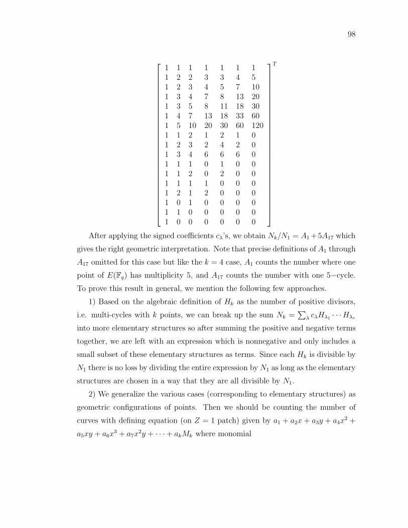
98

1 1 1 1 1 1 11 2 2 3 3 4 51 2 3 4 5 7 101 3 4 7 8 13 201 3 5 8 11 18 301 4 7 13 18 33 601 5 10 20 30 60 1201 1 2 1 2 1 01 2 3 2 4 2 01 3 4 6 6 6 01 1 1 0 1 0 01 1 2 0 2 0 01 1 1 1 0 0 01 2 1 2 0 0 01 0 1 0 0 0 01 1 0 0 0 0 01 0 0 0 0 0 0

T

After applying the signed coefficients cλ’s, we obtain Nk/N1 = A1 +5A17 which

gives the right geometric interpretation. Note that precise definitions of A1 through

A17 omitted for this case but like the k = 4 case, A1 counts the number where one

point of E(Fq) has multiplicity 5, and A17 counts the number with one 5−cycle.

To prove this result in general, we mention the following few approaches.

1) Based on the algebraic definition of Hk as the number of positive divisors,

i.e. multi-cycles with k points, we can break up the sum Nk =∑

λ cλHλ1 · · ·Hλr

into more elementary structures so after summing the positive and negative terms

together, we are left with an expression which is nonnegative and only includes a

small subset of these elementary structures as terms. Since each Hk is divisible by

N1 there is no loss by dividing the entire expression by N1 as long as the elementary

structures are chosen in a way that they are all divisible by N1.

2) We generalize the various cases (corresponding to elementary structures) as

geometric configurations of points. Then we should be counting the number of

curves with defining equation (on Z = 1 patch) given by a1 + a2x+ a3y + a4x2 +

a5xy + a6x3 + a7x

2y + · · ·+ akMk where monomial

99

Mk =

1 if k = 1

xk2 if 2|k

xk−32 y if 2 6 |k and k ≥ 3

.

Each of the terms in the expansion of Nk/N1 according to partitions signifies a

way of designating a subset of such curves, with some curves being designated

multiple times with different data. Then an inclusion-exclusion argument or alge-

braic formula for such multiplicities should be able to prove that Nk/N1 equals a

nonnegative sum of a small subset of the terms with the right form.

We obtain general expressions Nk = N1 · |Vk| where Vk equals the variety of

points satisfying P + π(P ) + · · · + πk−1(P ) ≡ kP∞. This is called the trace-zero

variety in the literature, e.g. [Fre01]. We provide the following explicit proof of

this identity.

Proposition 4.56. We have

Nk/N1 =

∣

∣

∣

∣

Ker (1 + π + π2 + · · ·+ πk−1)

∣

∣

∣

∣

.

Proof. One can prove this result simply by observing

(1− πk) = (1− π)(1 + π + π2 + · · ·+ πk−1)

and since these maps are group homomorphisms, we obtain∣

∣

∣

∣

Ker (1− πk)

∣

∣

∣

∣

=

∣

∣

∣

∣

Ker(1− π)

∣

∣

∣

∣

·∣

∣

∣

∣

Ker (1 + π + π2 + · · ·+ πk−1)

∣

∣

∣

∣

, i.e

Nk = N1 ·∣

∣

∣

∣

Ker (1 + π + π2 + · · ·+ πk−1)

∣

∣

∣

∣

.

In the literature, this is also commonly cited by appealing to Weil descent or

Weil restriction. Because of the importance of this particular variety, we provide

a second elementary proof of this equality.

Alternate proof of Corollary 4.56. Since π(P∞) = P∞ = π−1(P∞), we have that

any element P in the kernel of Trk = 1 + π + · · ·+ πk−1 must also satisfy

(1 + π + · · ·+ πk−1)π(P ) = (π + π2 + · · ·+ πk)(P ) = P∞.

100

Putting these two together, we get that such a P will satisfy (1−πk)(P ) = P∞. In

particular, P ∈ E(Fqk), and we conclude Ker Trk ⊆ E(Fqk). On the other hand, if

R is in the image of 1 + π + · · ·+ πk−1 acting on Q ∈ E(Fqk), then

(1 + π + · · ·+ πk−1)π(Q) = (π + π2 + · · ·+ πk)(Q) = (1 + π + · · ·+ πk−1)(Q),

hence (1− π)R = P∞, i.e. R ∈ E(Fq), and so Im Trk ⊆ E(Fq).

We wish to prove the following sequence

0 −→ Ker (1 + π + · · ·+ πk−1) −→ E(Fqk)1+π+···+πk−1

−−−−−−−−−−→E(Fq) −→ 0

is exact; which would imply

|E(Fqk)||E(Fq)|

=

∣

∣

∣

∣

Ker (1 + π + π2 + · · ·+ πk−1)

∣

∣

∣

∣

.

The only part we have left to prove is the fact that Trk : E(Fqk) → E(Fq) is

surjective. This can be verified by Hilbert’s Theorem 90. [DF91].

Theorem 4.57 (Additive Version of Hilbert’s Theorem 90). Let L/K be a finite

cyclic Galois extension (of degree k) with Gal(L/K) = 〈σ〉. An element y ∈ L

satisfies

∑

τ∈Gal(L/K)

τ(y) =

k−1∑

i=0

σi(y) = φk(y) = 0

if and only if there exists x ∈ L such that y = x− σ(x).

By this Theorem, we rephrase the problem of finding the image of Trk as

finding the kernel of operator 1− π, which is E(Fq). However, we can also prove

surjectivity by elementary means, as done in [GM, Ch. 1] for Fqk −→Trk Fq. We

thus use this proof by considering how π : E(Fqk) → E(Fqk) acts on each of two

coordinates. By abuse of notation we now use π to denote the map from Fqk 7→ Fqk

which sends α to αq. Similarly Trk will be 1 + π+ π2 + · · ·+ πk−1. The trace map

is linear over Fq, satisfying Trk(c1α+c2β) = c1Trk(α)+c2Trk(β) for all c1, c2 ∈ Fq

and α, β ∈ Fqk . Also we have that for α ∈ Fqk the property

Trk(αx) = 0 for all x ∈ Fqk if and only if α = 0

101

since the equation Trk(x) = 0 is of degree qk−1 and thus cannot have more than

qk−1 solutions in Fqk . Since Fqk has qk elements, we can certainly find α ∈ Fqk

such that Trk(α) 6= 0. Thus we let Trk(α) = c1 for c1 ∈ Fq \ {0}, and by using

linearity of the trace map, we have Trk(c2α/c1) = c2 for all c2 ∈ Fq . Thus

Trk = 1 + π + π2 + · · ·+ πk−1 is surjective from Fqk onto Fq.

While the author has not worked out the details, this numeric identity should

also give rise an explicit bijection for higher k via coset decomposition, as in the

k = 2 case. Unfortunately, as seen even in that case, hope for a natural bijection

is doubtful since the most natural type of bijection, a group isomorphism, cannot

be constructed in general.

4.5 Acknowledgement

Much of the material in Chapter 4 has been submitted for publication in the

paper “Combinatorial Aspects of Elliptic Curves” by Gregg Musiker. The disser-

tation author is the primary investigator and author of this paper.

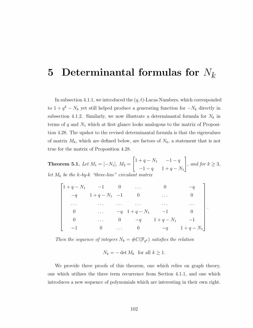
5 Determinantal formulas for Nk

In subsection 4.1.1, we introduced the (q, t)-Lucas Numbers, which corresponded

to 1 + qk − Nk yet still helped produce a generating function for −Nk directly in

subsection 4.1.2. Similarly, we now illustrate a determinantal formula for Nk in

terms of q and N1 which at first glance looks analogous to the matrix of Proposi-

tion 4.28. The upshot to the revised determinantal formula is that the eigenvalues

of matrix Mk, which are defined below, are factors of Nk, a statement that is not

true for the matrix of Proposition 4.28.

Theorem 5.1. Let M1 = [−N1], M2 =

[

1 + q −N1 −1− q−1− q 1 + q −N1

]

, and for k ≥ 3,

let Mk be the k-by-k “three-line” circulant matrix

1 + q −N1 −1 0 . . . 0 −q−q 1 + q −N1 −1 0 . . . 0

. . . . . . . . . . . . . . . . . .

0 . . . −q 1 + q −N1 −1 0

0 . . . 0 −q 1 + q −N1 −1

−1 0 . . . 0 −q 1 + q −N1

.

Then the sequence of integers Nk = #C(Fqk) satisfies the relation

Nk = − detMk for all k ≥ 1.

We provide three proofs of this theorem, one which relies on graph theory,

one which utilizes the three term recurrence from Section 4.1.1, and one which

introduces a new sequence of polynomials which are interesting in their own right.

102

103

5.1 First proof of Theorem 5.1: Via graph theory

In subsection 4.1.3, we proved that Nk can be written as −Wk(q,−N1) where

Wk is a (q, t)-analogue of the number of spanning trees of Wk, where each tree

is given a certain (q, t)-weighting. An alternative definition of Wk(q, t) uses a

deformation of the wheel graph such that each edge incident to the central hub is

replaced with t bi-directed edges, and every two adjacent vertices along the rim

are connected via q edges going clockwise and 1 edge going counter-clockwise.

q2t3

dist = 1

dist = 1

dist = 0

t = 2q = 3

Figure 5.1: A second definition of Wk(q, t).

With this definition of the (q, t)-Wk, we no longer have to weight the spanning

trees to obtain Wk(q, t); instead the (q, t)-weighting is implicit in the definition of

the (q, t)-wheel graph. More precisely we obtain

Lemma 5.2. Wk(q, t) as defined in Section 4.13 is equal to the (without weighting)

number of directed rooted spanning trees of (q, t)-Wk which are rooted at the central

hub.

104

Having dispensed with the weightings, we can appeal to the directed multi-

graph version of the Matrix-Tree Theorem to count (in the ordinary sense) the

number of spanning trees of (q, t)-Wk with root v0. Before describing this theorem,

we provide some necessary terminology that will also be used again in Chapter 6.

A directed multi-graph, as the name and picture implies, is a directed version of

the simple graphs we earlier defined which also allow multiple edges between a

given pair of vertices. We call the number of outgoing edges of a given vertex, the

outdegree, and denote this quantity as d(vi). Additionally, we will let d(vi, vj)

denote the number of directed edges from vi to vj . The Laplacian matrix L of a

graph is defined by entries Lii = d(vi) and Li,j = −d(vi, vj). Finally we define a

rooted spanning tree, with root v0, to be an oriented spanning tree such that all

edges flow away from v0.

Theorem 5.3 (Matrix-Tree Theorem). The number of rooted spanning trees, with

root v0, of graph G is given as the determinant of the matrix L0 where L0 is the

reduced Laplacian matrix, i.e. matrix L with the column and row corresponding to

root v0 removed.

Proof. See [Sta99, Ch. 5].

In the case of the (q, t)-wheel graph Wk, we obtain Laplacian matrix

L =

1 + q + t −1 0 . . . 0 −q −t−q 1 + q + t −1 0 . . . 0 −t. . . . . . . . . . . . . . . . . . −t0 . . . −q 1 + q + t −1 0 −t0 . . . 0 −q 1 + q + t −1 −t−1 0 . . . 0 −q 1 + q + t −t−t −t −t . . . −t −t kt

where the last row and column correspond to the hub vertex, which happens to

be the root. By the Matrix-Tree theorem, the number of directed rooted spanning

trees is detL0 where L0 is matrix L with the last row and last column deleted. We

105

have the identities

Nk = −Wk(q,−N1) (5.1)

Mk = L0

∣

∣

∣

∣

t=−N1

and thus (5.2)

Wk(q, t) = detL0 implies (5.3)

−Wk(q,−N1) = − detL0

∣

∣

∣

∣

t=−N1

so we get (5.4)

Nk = − detMk. (5.5)

Thus we have proven Theorem 5.1.

5.1.1 The Smith normal form of matrices Mk

Before discussing the other proofs of Theorem 5.1, and related topics, we stop to

discuss a combinatorially interesting feature of these matrices. As we have written

the Mk’s, they are sparse circulant matrices with very simple entries. However, the

Smith normal forms of these matrices are also quite nice. Recall that the Smith

normal form of an integral matrix is unchanged by

1. Multiplication of a row or a column by −1.

2. Addition of an integer multiple of a row or column to another.

3. Swapping of two rows or two columns.

In particular, the determinant of the matrix is unchanged by these operations. To

be precise a matrix has a Smith normal form when its entries are defined over a

principal ideal domain R such as Z or F [x] where F is a field. In general, operation

(1) would be expressed as “multiplication of a row or a column by a unit in R,”

however when R = Z the only units are ±1. The matrices we consider have entries

which are integral polynomials in the constants q and N1 (or t). Thus to obtain

the Smith normal form, we must fix q and N1 (resp. t) to be specific integers

before proceeding. Nonetheless, even with this caveat, we will be able to provide

a combinatorial description of the Smith normal form of our matrices.

106

Theorem 5.4. The Smith normal form of Mk is equivalent to

1 0 . . . 0 0 0

0 1 . . . 0 0 0

. . . . . . . . . . . . . . . . . .

0 0 . . . 1 0 0

0 0 . . . 0 qEk−1/N1 − 1 −qEk/N1

0 0 . . . 0 Ek/N1 −Ek+1/N1 − 1

where the Ek’s are the signed bivariate Fibonacci polynomials from subsection 4.2.

Note that the lower-right 2-by-2 block will reduce to

[

m1 0

0 m2

]

such that m1|m2 as

integers once q and N1 are evaluated as specific numbers.

Before proving this theorem, we provide the following Lemma that will be a key

step in our proof. This Lemma describes a matrix identity which is an immediate

corollary to Proposition 4.20.

Lemma 5.5.

[

0 −q1 1 + q −N1

]n

=

[

q · (−1)n−1En−1/N1 q · (−1)nEn/N1

(−1)n−1En/N1 (−1)nEn+1/N1

]

for all n ≥ 2.

Proof. We prove this by induction on n. The initial conditions

[

0 −q

1 1 + q − N1

]2

=

[

−q −q(1 + q − N1)

1 + q − N1 (1 + q − N1)2 − q

]

=

[

−q · E1/N1 q · E2/N1

−E2/N1 E3/N1

]

[

0 −q

1 1 + q − N1

]3

=

[

−q(1 + q − N1) q2 − q(1 + q − N1)2

−q + (1 + q − N1)2 −E4/N1

]

=

[

q · E2/N1 −q · E3/N1

E2/N1 −E4/N1

]

are clear. Furthermore,

[

0 −q1 1 + q −N1

]

×[

q · (−1)n−1En−1/N1 q · (−1)nEn/N1

(−1)n−1En/N1 (−1)nEn+1/N1

]

=

[

q · (−1)nEn/N1 q · (−1)n+1En+1/N1

a2 b2

]

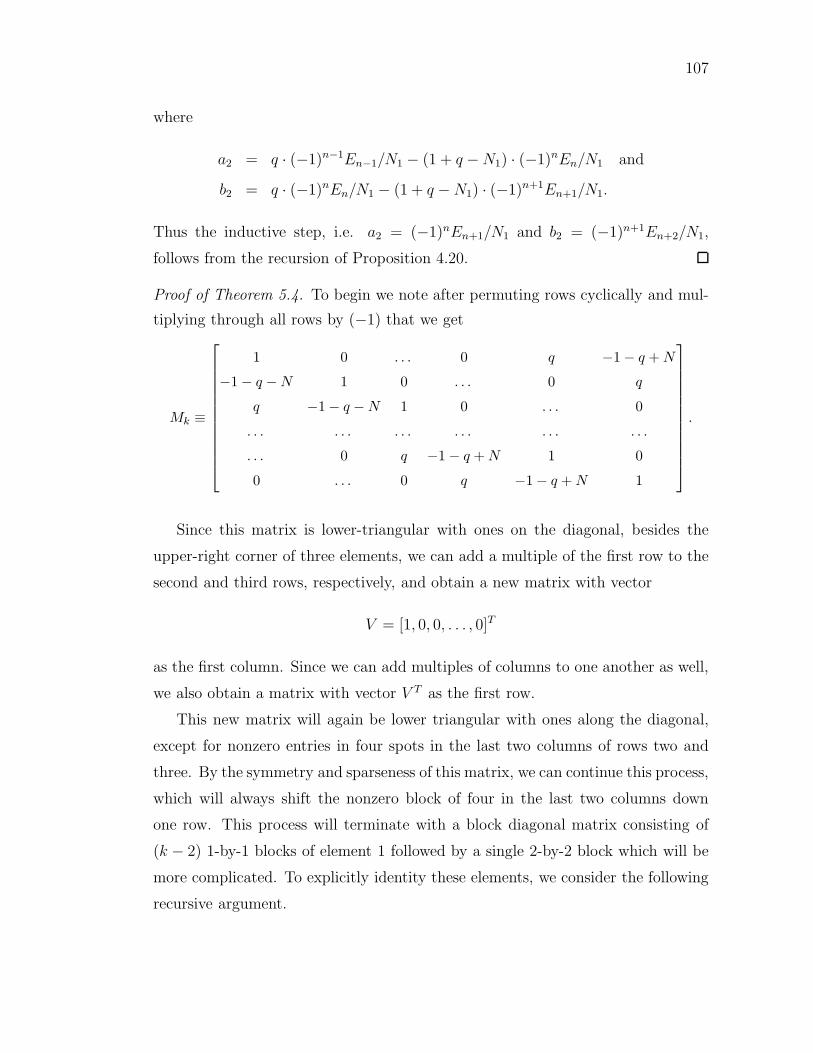
107

where

a2 = q · (−1)n−1En−1/N1 − (1 + q −N1) · (−1)nEn/N1 and

b2 = q · (−1)nEn/N1 − (1 + q −N1) · (−1)n+1En+1/N1.

Thus the inductive step, i.e. a2 = (−1)nEn+1/N1 and b2 = (−1)n+1En+2/N1,

follows from the recursion of Proposition 4.20.

Proof of Theorem 5.4. To begin we note after permuting rows cyclically and mul-

tiplying through all rows by (−1) that we get

Mk ≡

1 0 . . . 0 q −1− q + N

−1− q −N 1 0 . . . 0 q

q −1− q −N 1 0 . . . 0

. . . . . . . . . . . . . . . . . .

. . . 0 q −1− q + N 1 0

0 . . . 0 q −1− q + N 1

.

Since this matrix is lower-triangular with ones on the diagonal, besides the

upper-right corner of three elements, we can add a multiple of the first row to the

second and third rows, respectively, and obtain a new matrix with vector

V = [1, 0, 0, . . . , 0]T

as the first column. Since we can add multiples of columns to one another as well,

we also obtain a matrix with vector V T as the first row.

This new matrix will again be lower triangular with ones along the diagonal,

except for nonzero entries in four spots in the last two columns of rows two and

three. By the symmetry and sparseness of this matrix, we can continue this process,

which will always shift the nonzero block of four in the last two columns down

one row. This process will terminate with a block diagonal matrix consisting of

(k − 2) 1-by-1 blocks of element 1 followed by a single 2-by-2 block which will be

more complicated. To explicitly identity these elements, we consider the following

recursive argument.

108

Let

a′′1 b′′1

a′2 b′2

a3 b3

a4 b4

a5 b5...

...

ak bk

signify the last two columns of matrix Mk. Following the above

construction, we obtain

0 0

a′′2 b′′2

a′3 b′3

a4 b4

a5 b5...

...

ak bk

after one iteration, and

0 0

0 0

a′′3 b′′3

a′4 b′4

a5 b5...

...

ak bk

after the next, where

a′′i = (1 + q −N1)a′′i−1 + a′i

b′′i = (1 + q −N1)b′′i−1 + b′i

a′i+1 = −qa′′i−1 + ai+1

b′i+1 = −qb′′i−1 + bi+1

for 2 ≤ i ≤ k − 1. Consequently,

[

a′′m

a′′m+1

]

=

[

0 1

−q 1 + q −N1

][

a′′m−1

a′′m

]

+

[

0

am+1

]

and (5.6)

[

b′′m

b′′m+1

]

=

[

0 1

−q 1 + q −N1

][

b′′m−1

b′′m

]

+

[

0

bm+1

]

. (5.7)

Since we have a′′1 = q, b′′1 = −1− q +N1, b′2 = q, ak−1 = 1, ak = −1− q +N1,

109

bk = 1, and the rest of the ai and bi equal 0, we obtain[

a′′k−2

a′′k−1

]

=

[

0 1

−q 1 + q −N1

]k−3 [

a′′1

a′′2

]

+

[

0

ak−1

]

=

[

0 1

−q 1 + q −N1

]k−3 [

q

q(1 + q −N1)

]

+

[

0

1

]

.

Analogously,[

b′′k−2

b′′k−1

]

=

[

0 1

−q 1 + q −N1

]k−3 [

b′′1

b′′2

]

+

[

0

bk−1

]

=

[

0 1

−q 1 + q −N1

]k−3 [

−1− q +N1

q − (1 + q −N1)2

]

+

[

0

0

]

.

Putting this together we get

a′′k−2 b′′k−2

a′′k−1 b′′k−1

=

0 1

−q 1 + q −N1

k−3

q −1− q + N1

−1− q + N1 q − (1 + q −N1)2

+

0 0

1 0

which simplifies to[

a′′k−2 b′′k−2

a′′k−1 b′′k−1

]

= (−1)

[

0 1

−q 1 + q −N1

]k−1

+

[

0 0

1 0

]

.

Finally we get[

a′′k−1 b′′k−1

a′′k b′′k

]

= (−1)

[

0 1

−q 1 + q −N1

]k

+

[

0 1

−q 1 + q −N1

][

0 0

1 0

]

+

[

0 ak

0 bk

]

= (−1)

[

0 1

−q 1 + q −N1

]k

+

[

1 0

0 1

]

.

At this point we recall Lemma 5.5 which states[

0 −q1 1 + q −N1

]k

=

[

q · (−1)k−1Ek−1/N1 q · (−1)kEk/N1

(−1)k−1Ek/N1 (−1)kEk+1/N1

]

for all k ≥ 2. To finish the proof we multiply the last two rows by a power of (−1)

and take the transpose, neither of which effects the Smith normal form.

Besides showing another connection between the Fibonacci numbers and the

Nk’s, this theorem will be used again in Chapter 6.

110

5.2 Second proof of Theorem 5.1: Using orthog-

onal polynomials

Recall from the zeta function of an elliptic curve, Z(E, T ), we derived a three

term recurrence relation for the sequence {Gk = 1 + qk −Nk}:

Gk+1 = (1 + q −N1)Gk − qGk−1. (5.8)

Such a relation is indicative of an interpretation of the 1 + qk−Nk’s as a sequence

of orthogonal polynomials. In particular, any sequence of orthogonal polynomials,

{Pk(x)}, satisfies

Pk+1(x) = (akx+ bk)Pk(x) + ckPk−1(x) (5.9)

where ak, bk and ck are constants that depend on k ∈ N. Additionally, it is usual

to initialize P−k(x) = 0, P0(x) = 1, and P1(x) = a0x+ b0.

Since we can think of the bivariate Nk(q,N1) as univariate polynomials in

variable N1 with constants from field Q(q), it follows that recurrence (5.8) is such

an example, with

ak = −1 for k ≥ 0

bk = 1 + q for k ≥ 0,

c1 = −2q and

ck = −q for k ≥ 2

in the case. (Note that we must take c1 to be 2q because we originally defined

L0(q, t) as 2.) One of the properties of a sequence of orthogonal polynomials is an

interpretation as the determinants of a family of tridiagonal k-byk matrices. In

particular, we obtain a second proof of Proposition 4.28.

Proof. Given a sequence of orthogonal polynomials satisfying P0(x) = 1, P1(x) =

111

a0x+ b0 and recurrence (5.9), we have the formula [IPS00]

Pk(x) = det

a0x+ b0 c1 0 0 0 0

−1 a1x+ b1 c2 0 0 0

0 −1 a2x+ b2 c3 0 0...

......

. . .. . . 0

0 0 0 · · · ak−2x+ bk−2 ck

0 0 0 · · · −1 ak−1x+ bk−2

.

Plugging in the ai, bi, and ci’s as above yields the formula.

Recall that we obtained these same formulas, i.e. determinants of matrices M ′k

in Section 4.2. We can prove Theorem 5.1 by an algebraic manipulation of matrix

Mk followed by use of Proposition 4.28. Namely, by using the multilinearity of the

determinant, and expansions about the first row followed by the first column, we

obtain

det(Mk) = det(Ak) + det(Bk) + det(Ck) + det(Dk)

where Ak, Bk, Ck, and Dk are the following k-by-k matrices:

Ak =

1 + q −N1 −1 0 0 0 0

−q 1 + q −N1 −1 0 0 0

0 −q 1 + q −N1 −1 0 0...

......

. . .. . . 0

0 0 0 · · · 1 + q −N1 −1

0 0 0 · · · −q 1 + q −N1

.

Bk =

0 0 0 0 0 −q−q 1 + q −N1 −1 0 0 0

0 −q 1 + q −N1 −1 0 0...

......

. . .. . . 0

0 0 0 · · · 1 + q −N1 −1

0 0 0 · · · −q 1 + q −N1

.

112

Ck =

0 −1 0 0 0 0

0 1 + q −N1 −1 0 0 0

0 −q 1 + q −N1 −1 0 0...

......

. . .. . . 0

0 0 0 · · · 1 + q −N1 −1

−1 0 0 · · · −q 1 + q −N1

.

Dk =

0 0 0 0 0 −q0 1 + q −N1 −1 0 0 0

0 −q 1 + q −N1 −1 0 0...

......

. . .. . . 0

0 0 0 · · · 1 + q −N1 −1

−1 0 0 · · · −q 1 + q −N1

.

Cyclic permutation of the rows of Bk and the columns of Ck yield upper-triangular

matrices with −1’s (resp. −q)’s on the diagonal. Given that the sign of such a

cyclic permutation is (−1)k−1, we obtain det(Bk)+det(Ck) = −q−1. Additionally,

by expanding det(Dk) about the first row followed by the first column, we obtain

det(Dk) = −q det(Ak−2). In conclusion

1 + qk + det(Mk) = det(Ak)− q det(Ak−2).

By analogous methods we obtain

detM ′k = det(Ak)− q det(Ak−2)

and thus the desired formula detMk = −Nk.

5.2.1 Explicit connection to orthogonal polynomials

We now push the analysis of the last section further, writing the {1+qk−Nk}’sexplicitly in terms of a sequence of classical orthogonal polynomials. We let Tk(x)

denote the kth Chebyshev (Tchebyshev) polynomials of the first kind, which are

113

defined as cos(kθ) written out in terms of x such that θ = arccos x. Equivalently,

we can define Tk(x) as the expansion of αk + βk in terms of powers of cos θ where

α = cos θ + i sin θ

β = cos θ − i sin θ.

Theorem 5.6. Considering the (1 + qk − Nk)’s as univariate polynomials in N1

over the field Q(q), we obtain

1 + qk −Nk = 2qk/2Tk

(

(1 + q −N1)/2q1/2

)

.

Proof. We note that Chebyshev polynomials satisfy initial conditions T0(x) = 1,

and T1(x) = x and the three-term recurrence

Tk+1(x) = 2xTk(x)− Tk−1(x)

for k ≥ 1 since

Tk+1(x) = αk+1 + βk+1

= (α+ β)(αk + βk)− αβ(αk−1 + βk−1)

= 2 cos θ Tk(x)− Tk−1(x)

= 2xTk(x)− Tk−1(x).

Let x = 1+q−N1

2√

q. Clearly Theorem 5.6 holds for k = 1, and additionally the

1+qk−Nk

2qk/2 ’s satisfy the same recurrence as the Tk(x)’s. Namely

1 + qk+1 −Nk+1

2q(k+1)/2=

(1 + q −N1)(1 + qk −Nk)− q(1 + qk−1 −Nk−1)

2q(k+1)/2

= 2

(

1 + q −N1

2q1/2

)(

1 + qk −Nk

2qk/2

)

−(

1 + qk−1 −Nk−1

2q(k−1)/2

)

.

Another way to foresee the appearance of Chebyshev polynomials is by noting

that in the case that we plug in q = 0 or q = 1, we obtain a family of univariate

polynomials Nk with the property Nmk = Nm(Nk) = Nk(Nm). It is a fundamental

theorem of Chebyshev polynomials that families of univariate polynomials with

114

such a property are very restrictive. In particular, from [BT51] as described on

page 33 of [BE95]: If {Nk} is a sequence of integral univariate polynomials of

degree k with the property

Nmn = Nm(Nn) = Nn(Nm)

for all positive integers m and n, then Nk must either be a linear transformation

of

1. xk or

2. Tk(x), the Chebyshev polynomial of the first kind,

where a linear transformation of a polynomial f(x) is of the form

A · f(

(x− B)/A

)

+B or equivalently

(

f(Ax+B)− B)/

A.

In particular we get formulas forWk(0, N1) andWk(1, N1) (resp. Nk(0, N1) and

Nk(1, N1)) which are indeed linear transformations of xk and Tk(x) respectively.

Proposition 5.7.

Nk(0, N1) = −(1−N1)k + 1, (5.10)

Nk(1, N1) = −2Tk(−N1/2 + 1) + 2. (5.11)

Proof. The coefficient of Nm1 inWk(0, N1) is the number of directed spanning trees

of Wk with m spokes and arcs always directed counter-clockwise. In particular it

is only the placement of the spokes that matter at this point since the placement

of the arcs is now forced. Thus the coefficient of Nm1 in Wk(0, N1) is

(

km

)

for all

1 ≤ m ≤ k. Thus the generating function Wk(0, N1) satisfies

Wk(0, N1) = (1 +N1)k − 1

since the constant term of Wk(0, N1) is zero. Using the relation Nk(q,N1) =

−Wk(q,−N1) completes the proof in the q = 0 case. We also note that −(1−x)k+1

is a linear transformation of xk via A = −1 and B = 1. The case for q = 1 is a

corollary of Theorem 5.6.

115

For higher values of q, we lose some of the symmetry and thus cannot apply

the Fundamental Theorem of Chebyshev polynomials. However, it seems fruit-

ful to consider the theory of Chebyshev polynomials when considering alternate

polynomial expressions or expansions ofWk(q,N1). For example, putting together

Proposition 5.7 with a result of [ZYG05], namely Theorem 12, we get the following

result.

Theorem 5.8. For n = N1 ≥ k ≥ 3, let T (Kn−Ck) signify the number of spanning

trees in the graph Kn − Ck formed by taking the complete graph on n vertices and

removing the k edges of a k-cycle. Then we have as a formal expression

T (Kn − Ck) = (−1)k−1nn−k−2Nk(1, n).

Proof. In [ZYG05], the authors develop a formula in terms of Chebyshev polyno-

mials for the number of spanning trees of various graphs. In particular, they find

that

T (Kn − Ck) = nn−k−2

[(√

n

4+

√

n− 4

4

)k

−(

−√

n

4+

√

n− 4

4

)k]2

which after several steps of algebra is found to be equal to

nn−k−2(−1)k(2Tk(−n/2 + 1)− 2).

More specifically, we use relation

Tk(x) =1

2

[(

x+√x2 − 1

)k

+

(

x−√x2 − 1

)k]

from Equation (19) of [BP86]. Plugging in x = −n/2 + 1, we get

(−1)k

(

2Tk(−n/2 + 1)− 2

)

=

(

n/2− 1−√

n(n− 4)

4

)k

+

(

n/2− 1 +

√

n(n− 4)

4

)k

+ 2(−1)k−1.

On the other hand, expanding

[(√

n

4+

√

n − 4

4

)k

−(

−√

n

4+

√

n − 4

4

)k]2

=

(√

n

4+

√

n − 4

4

)2k

+

(

−√

n

4+

√

n − 4

4

)2k

− 2

(√

n

4+

√

n − 4

4

)k(

−√

n

4+

√

n − 4

4

)k

,

116

we obtain

−2

(√

n

4+

√

n− 4

4

)k(

−√

n

4+

√

n− 4

4

)k

= −2

(

n− 4

4− n

4

)k

= 2(−1)k−1

and

(√

n

4+

√

n− 4

4

)2k

=

(

n

4+2

√

n(n− 4)

16+n− 4

4

)k

=

(

n/2−1+

√

n(n− 4)

4

)k

.

Analogously

(

−√

n

4+

√

n− 4

4

)2k

=

(

n

4−2

√

n(n− 4)

16+n− 4

4

)k

=

(

n/2−1−√

n(n− 4)

4

)k

.

We thus have T (Kn − Ck) = nn−k−2(−1)k

(

2Tk(−N1/2 + 1) − 2

)

which equals

nn−k−2(−1)k

(

−Nk(1, n)

)

by Proposition 5.7.

5.3 Third proof of Theorem 5.1: Using the zeta

function

Alternatively, we note that we can factor

Nk = 1 + qk − αk1 − αk

2

using the fact that q = α1α2. Consequently,

Nk = (1− αk1)(1− αk

2)

and we can factor each of these two terms using cyclotomic polynomials. We recall

that (1− xk) factors as

1− xk =∏

d|kCycd(x)

where Cycd(x) is a monic irreducible polynomial with integer coefficients. We can

similarly factor Nk as

Nk =∏

d|kCycd(α1)Cycd(α2).

117

These factors are therefore bivariate analogues of the cyclotomic polynomi-

als, and we will refer to them henceforth as elliptic cyclotomic polynomials,

denoted as ECycd.

Definition 5.9. We define the elliptic cyclotomic polynomials to be a sequence of

polynomials in variables q and N1 such that for d ≥ 1,

ECycd = Cycd(α1)Cycd(α2),

where α1 and α2 are the two roots of

T 2 − (1 + q −N1)T + q.

We verify that they can be expressed in terms of q and N1 by the following propo-

sition.

Proposition 5.10. Writing down ECycd in terms of q and N1 yields irreducible

bivariate polynomials with integer coefficients.

Proof. Firstly we have

αj1 + αj

2 = (1 + qj −Nj) ∈ Z

for all j ≥ 1 and expanding a polynomial in α1 multiplied by the same polynomial

in α2 yields terms of the form αi1α

i2(α

j1 + αj

2). Secondly the quantity Nj is an

integral polynomial in terms of q and N1 by Theorem 4.1 and αi1α

i2 = qi. Putting

these relations together, and the fact that Cycd is an integral polynomial itself, we

obtain the desired expressions for ECycd.

Now let us assume that ECycd is factored as F (q,N1)G(q,N1). The polynomial

Cycd(x) factors over the complex numbers as

Cycd(x) =d∏

j=1

gcd(j,d)=1

(1− ωjx)

where ω is a dth root of unity. Thus F (q,N1) =∏

i∈S(1−ωiα1)∏

j∈T (1−ωjα2) for

some nonempty subsets S, T of elements relatively prime to d. The only way F can

be integral is if F equals its complex conjugate F . However, α1 and α2 are complex

118

conjugates by the Riemann hypothesis for elliptic curves [Has34, Sil92] (Hasse’s

Theorem), and thus F = F implies that the sets S and T are equal. Since Cycd(x)

is known to be irreducible, the only possibility is S = T = {j : gcd(j, d) = 1}, and

thus F (q,N1) = ECycd, G(q,N1) = 1.

Remark 5.11. Alternatively, the integrality of the ECycd’s follows from the Funda-

mental Theorem of Symmetric Functions that states that a symmetric polynomial

with integer coefficients can be rewritten as an integral polynomial in e1, e2, . . . .

In this case, Cycd(α1)Cycd(α2) is a symmetric polynomial in two variables so

e1 = α1 +α2 = 1+q−N1, e2 = α1α2 = q, and ek = 0 for all k ≥ 3. Thus we obtain

an expression for ECycd as a polynomial in q and N1 with integer coefficients.

We can factor Nk, i.e. the ECycd’s even further, if we no longer require our

expressions to be integral.

Nk =

k∏

j=1

(1− α1ωjk)(1− α2ω

jk)

=

k∏

j=1

(1− (α1 + α2)ωjk + (α1α2)ω

2jk )

= (−1)

k∏

j=1

(−ωk−jk )(1− (1 + q −N1)ω

jk + (q)ω2j

k )

= −k∏

j=1

(

(1 + q −N1)− qωjk − ω

k−jk

)

.

Furthermore, the eigenvalues of a circulant matrix are well-known, and involve

roots of unity analogous to the expression precisely given by the second equation

above. (For example Loehr, Warrington, and Wilf [LWW04] provide an analy-

sis of a more general family of three-line-circulant matrices from a combinatorial

perspective. Using their notation, our result can be stated as

Nk = Φk,2(1 + q −N1,−q)

where Φp,q(x, y) =∏p

j=1(1 − xωj − yωqj) and ω is a primitive pth root of unity.

It is unclear how our combinatorial interpretation of Nk, in terms of spanning

trees, relates to theirs, which involves permutation enumeration.) In particular,

119

we prove Theorem 5.1 since detMk equals the product of Mk’s eigenvalues, which

are precisely given as the k factors of −Nk in second equation above.

5.3.1 Combinatorics of elliptic cyclotomic polynomials

In this subsection we further explore properties of elliptic cyclotomic polyno-

mials, noting that they are more than auxiliary expressions that appear in the

derivation of a proof. To start with, by Mobius inversion, we can use the identity

Nk =∏

d|kECycd(q,N1) (5.12)

to define elliptic cyclotomic polynomials directly as

ECyck(q,N1) =∏

d|kN

µ(k/d)d (5.13)

in addition to the alternative definition

ECyck(q,N1) =k∏

j=1

gcd(j,d)=1

(

(1 + q −N1)− qωjk − ω

k−jk

)

. (5.14)

In particular, ECyc1 = N1 and ECycp = Np/N1 if p is prime. We note several

commonalities among these polynomials, as described in the following propositions.

These properties are further rationale for our choice of name for this family of

polynomials.

Proposition 5.12. We have

ECycd|N1=0 = C(d)Cycd(q) (5.15)

ECycd|N1=2q+2 = C ′(d)Cycd(−q) (5.16)

where C(d) and C ′(d) are the functions from Z>0 to Z≥0 such that

C(d) =

0 if d = 1

p if d = pk for p prime

1 otherwise

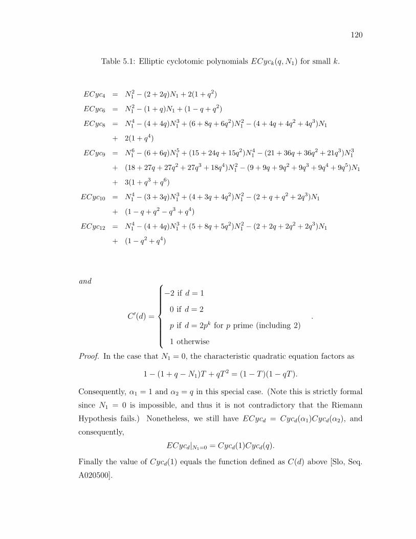
120

Table 5.1: Elliptic cyclotomic polynomials ECyck(q,N1) for small k.

ECyc4 = N21 − (2 + 2q)N1 + 2(1 + q2)

ECyc6 = N21 − (1 + q)N1 + (1− q + q2)

ECyc8 = N41 − (4 + 4q)N3

1 + (6 + 8q + 6q2)N21 − (4 + 4q + 4q2 + 4q3)N1

+ 2(1 + q4)

ECyc9 = N61 − (6 + 6q)N5

1 + (15 + 24q + 15q2)N41 − (21 + 36q + 36q2 + 21q3)N3

1

+ (18 + 27q + 27q2 + 27q3 + 18q4)N21 − (9 + 9q + 9q2 + 9q3 + 9q4 + 9q5)N1

+ 3(1 + q3 + q6)

ECyc10 = N41 − (3 + 3q)N3

1 + (4 + 3q + 4q2)N21 − (2 + q + q2 + 2q3)N1

+ (1− q + q2 − q3 + q4)

ECyc12 = N41 − (4 + 4q)N3

1 + (5 + 8q + 5q2)N21 − (2 + 2q + 2q2 + 2q3)N1

+ (1− q2 + q4)

and

C ′(d) =

−2 if d = 1

0 if d = 2

p if d = 2pk for p prime (including 2)

1 otherwise

.

Proof. In the case that N1 = 0, the characteristic quadratic equation factors as

1− (1 + q −N1)T + qT 2 = (1− T )(1− qT ).

Consequently, α1 = 1 and α2 = q in this special case. (Note this is strictly formal

since N1 = 0 is impossible, and thus it is not contradictory that the Riemann

Hypothesis fails.) Nonetheless, we still have ECycd = Cycd(α1)Cycd(α2), and

consequently,

ECycd|N1=0 = Cycd(1)Cycd(q).

Finally the value of Cycd(1) equals the function defined as C(d) above [Slo, Seq.

A020500].

121

For the reader’s convenience we also provide a simple proof of this equality. It

is clear that Cyc1(q) = 1− q and Cycp(q) = 1+ q+ q2 + · · ·+ qp−1 so by induction

on k ≥ 1, assume that Cycpk(1) = p.

1− qpk

1− q = 1 + q + q2 + · · ·+ qpk−1 =k∏

j=1

Cycpj(q).

Plugging in q = 1, and by induction we get pk = pk−1 · Cycpk(1), thus we have

Cycpk(1) = p. We now proceed to show Cycd(1) = 1 if d = pk11 p

k22 · · · pkr

r for any

r ≥ 2. For this we use k such that d|k. We assume k = pk′1

1 pk′2

2 · · ·pk′

rr .

1− qk

1− q = 1 + q + q2 + · · ·+ qk−1

=

( k′1∏

j1=1

Cycp

j11

(q)

)( k′2∏

j2=1

Cycp

j22

(q)

)

· · ·( k′

r∏

jr=1

Cycpjrr

(q)

)

×(

∏

d is another divisor of k

Cycd(q)

)

.

The expression 1−qk

1−q

∣

∣

∣

∣

q=1

equals k, and the first r products on the right-hand-side

equal pk′1

1 , pk′2

2 , . . . , pk′

rr respectively. Thus the last set of factors, i.e. the cyclotomic

polynomials of d with two or more prime factors, must all equal the value 1.

We prove (5.16) analogously. When N1 = 2q+ 2 (again this is strictly formal),

the characteristic equation factors as

1− (1 + q −N1)T + qT 2 = (1 + T )(1 + qT )

implying α1 = −1 and α2 = −q. Additionally, C ′(d) = Cycd(−1) was observed by

Ola Veshta on Jun 01 2001, as cited on [Slo, Seq. A020513].

Proposition 5.13. For d ≥ 2,

degN1ECycd = degq ECycd = φ(d),

where the Euler φ function which counts the number of integers between 1 and d−1

which are relatively prime to d.

122

Proof. As noted in Remark 5.11, we can write ECycd as an integral polynomial

in e1 = α1 + α2 = 1 + q − N1 and e2 = α1α2 = q. The highest degree of N1 in

ECycd is therefore equal to the highest degree of e1 = α1+α2, which is the same as

the largest m such that αm1 α

02 (resp. α0

1αm2 ) is a term in Cycd(α1)Cycd(α2). Thus

degN1ECycd(q,N1) = degα1

Cycd(α1) = φ(d). Analogously, the degree of q comes

from the highest power of (α1α2)m in Cycd(α1)Cycd(α2). Thus we have shown

degq ECycd ≤ φ(d).

Equality follows from the first half of Proposition 5.12 when d ≥ 2 since the

constant term with respect to N1, which equals C(d)Cycd(q), has degree φ(d).

Finally, if one examines the expressions for ECycd(q,N1), one will note that

they appear alternating in sign just as the polynomials for Nk, except for the

constant term which equals C(d)Cycd(q) by Proposition 5.12. More precisely, the

author finds the following empirical evidence for such a claim:

Proposition 5.14. For d between 2 and 104, we obtain

ECycd(q,N1) = Cycd(1) · Cycd(q) +

φ(d)∑

i=1

(−1)iQi,d(q)Ni1

where Qi,d is a univariate polynomial with positive integer coefficients.

However, the conjecture fails for d = 105. In particular,

ECyc105(q,N1) = Cyc105(1) · Cyc105(q) +

φ(d)∑

i=1

(−1)iQi,d(q)Ni1

+

(

2q40 + 18q39 + 33q38 + 33q37 + 33q36 + 21q35 + 10q34

+ 10q13 + 21q12 + 33q11 + 33q10 + 33q9 + 18q8 + 2q7

)

N1

where the Qi,d’s are univariate polynomials with positive integer coefficients. (Note

that there are 46 coefficients of N1 in the expansion of ECyc105(q,N1), only 14 of

which have the unexpected sign.)

The number 105 = 3 · 5 · 7 is significant and interesting from a number theo-

retic point of view. This number is also the first d such that ordinary cyclotomic

polynomial Cycd has a coefficient other than −1, 0, or 1.

123

Cyc105 = 1 + x+ x2 − x5 − x6 − 2x7 − x8 − x9 + x12 + x13 + x14

+ x15 + x16 + x17 − x20 − x22 − x24 − x26 − x28 + x31 + x32

+ x33 + x34 + x35 + x36 − x39 − x40 − 2x41 − x42 − x43

+ x46 + x47 + x48.

Despite this counter-example, we still can prove that the coefficients of the

ECycd’s alternate in sign for an infinite number of d’s. Specifically, we note that

ECyc2m resemble the coefficients of N2m−1 , and moreover the pattern we find is

Proposition 5.15.

ECyc2m = 2Cyc2m−1(q)−N2m−1 . (5.17)

In particular, for i between 1 and φ(2m) = 2m−1, we get

Qi,2m = Pi,2m−1 (5.18)

where the Pi,k are the coefficients of Nk.

Note that in our proof we will use the fact that ECycd can be written as

Cycd(1) · Cycd(q) +

φ(d)∑

i=1

(−1)iQi,d(q)Ni1

where the Qi,d’s are univariate polynomials with possibly negative coefficients.

Therefore, our proof of Proposition 5.15 will actually extend Proposition 5.14 to

the case where d is a power of 2 since we previously showed that the Pi,d’s alternate.

Proof. We note that Cyc2m−1 = 1+q2m−1and that (5.18) follows from (5.17). Also,

ECyc2m = N2m/N2m−1 and thus it suffices to prove

N2m = (2 + 2q2m−1

)N2m−1 −N22m−1 .

However, this is a special case of

N2(q,N1) = (2 + 2q)N1(q,N1)−N1(q,N1)2

where we plug in q2m−1in the place of q.

124

Unfortunately, formulas for Qi,d’s in terms of Pi,k’s when d is not a power of

2 are not as simple. On the other hand, the last part of this proof highlights a

principle that has the potential to open up a new direction. Namely, Nk(q,N1) is

defined as the number of points on E(Fqk) where q itself can also be a power of p.

Consequently,

Nm·k(q, N1) = #E(Fqm·k) = Nm

(

qk, Nk

)

. (5.19)

While this relation is immediate given our definition of Nk = #E(Fqk), when we

translate this relation in terms of spanning trees, the relation

Wmk(q, t) =Wm

(

qk,Wk(q, t)

)

(5.20)

seems much more novel. Furthermore, in this case, this relation involves only

positive integer coefficients and thus motivates exploration for a bijective proof. As

noted in Section 5.2.1, such a compositional formula is indicative of the appearance

of a linear transformation of xk or Tk(x), which is also clear from the three-term

recurrence satisfied by the 1 + qk −Nk’s.

5.3.2 Geometric interpretation of elliptic cyclotomic poly-

nomials

Despite the fact that the above expressions of elliptic cyclotomic polynomials

do not have positive coefficients nor coefficients with alternating signs, we can

nonetheless describe a set of geometric objects which the elliptic cyclotomic poly-

nomials enumerate.

Theorem 5.16. We have

ECycd =

∣

∣

∣

∣

Ker

(

Cycd(π)

)

: E(Fq)→ E(Fq)

∣

∣

∣

∣

where π denotes the Frobenius map, and Cycd(π) is an element of End(E) =

End(E(Fq)).

Proof. One of the key properties of the Frobenius map is the fact that E(Fqk) =

Ker(1− πk), where 1− πk is an element of End(E). See [Sil92] for example. The

125

map (1 − πk) factors into cyclotomic polynomials in End(E) since the endomor-

phism ring contains both integers and powers of π.

Since the maps Cycd(π) are each group homomorphisms, it follows that the car-

dinality of

∣

∣

∣

∣

Ker

(

Cycd1Cycd2(π)

)∣

∣

∣

∣

equals

∣

∣

∣

∣

Ker Cycd1(π)

∣

∣

∣

∣

·∣

∣

∣

∣

Ker Cycd2(π)

∣

∣

∣

∣

. Thus

∏

d|kECycd = Nk =

∣

∣

∣

∣

Ker (1− πk)

∣

∣

∣

∣

=

∣

∣

∣

∣

Ker∏

d|kCycd(π)

∣

∣

∣

∣

=∏

d|k

∣

∣

∣

∣

Ker Cycd(π)

∣

∣

∣

∣

,

and since the last equation is true for all k ≥ 1, we must have the relations

ECycd =

∣

∣

∣

∣

Ker Cycd(π)

∣

∣

∣

∣

. (5.21)

for all d ≥ 1.

5.4 Acknowledgement

Much of the material in Chapter 5 has been submitted for publication in the

paper “Combinatorial Aspects of Elliptic Curves” by Gregg Musiker. The disser-

tation author is the primary investigator and author of this paper.

6 Connections between elliptic

curves and chip-firing

In Chapter 4 we explored elliptic curves from a combinatorial viewpoint, find-

ing that Nk = #E(Fqk), the number of points over Fqk , could be written as an

integral polynomial only depending on q and N1. This motivated the main topic

of that chapter, which was the search for a combinatorial interpretation of these

coefficients, one such interpretation involving spanning trees of wheel graphs.

In this chapter, we continue this journey. As discussed in Chapter 3, an elliptic

curve E has an abelian group structure, and in this chapter we describe a family

of abelian groups whose orders are given by the sequence {Wk(q,N1)}, i.e. groups

that are equinumerous with the weighted number of spanning trees of the wheel

graph.

6.1 Introduction to chip-firing games

We now step away from elliptic curves momentarily and discuss some funda-

mental results from the theory of chip-firing games on graphs. The main source for

these details is [Big99], though there is an extensive literature on the subject, for

example [Mer05, Wag00]. At first glance, this topic might appear totally unrelated

to elliptic curves, but we will shortly flesh out the connection. Given a directed

(loop-less) graph G, we define a configuration C to be a vector of nonnegative

integers, with a coordinate for each vertex of the graph, letting Ci denote the in-

teger corresponding to vertex vi. One can think of this assignment as a collection

of chips placed on each of the vertices. We say that a given vertex vi can fire if

126

127

the number of chips it holds, Ci, is greater than or equal to its out-degree. If so,

firing leads to a new configuration where a chip travels along each outgoing edge

incident to vi. Thus we obtain a configuration C ′ where C ′j = Cj + d(vi, vj) and

C ′i = Ci − d(vi). Here d(vi, vj) equals the number of directed edges from vi to vj ,

and d(vi) is the out-degree of vi, which of course equals∑

j 6=i d(vi, vj).

Many interesting problems arise from this definition. For example, it can be

shown [LP01] that the set of configurations reachable from an initial choice of

a vector forms a distributive lattice. Thus one can ask combinatorial questions

such as examining the structure of this lattice as a poset. Other computations

such as the minimal number or expected number of firings necessary to reach

configuration C ′ from C are also common in dynamical systems. In this field,

critical configurations are often referred to as the abelian sandpile model [Mer05].

In this classical model, we consider the Z-by-Z lattice, and presume we are given

an initial configuration where each lattice point (site) has a collection of grains of

sand on top of it. We further suppose that once a site contains ≥ 4 grains of sand,

it topples, sending one grain of sand to each of its neighbors. In this way, by adding

sand to this system at a given point, one can cause an avalanche. Namely that

particular pile of sand will topple onto its neighbors, which in turn might now have

too much sand and there will be a smoothing out process of this nature until an

equilibrium is achieved. This is known as the abelian sandpile model because if two

grains are added at two different sites, the resulting equilibrium is independent of

the order in which the grains are added. This same notion can be applied in more

generality for any graph where we place chips on the vertices, as we will shortly

discuss.

For the purposes of relating this topic to an elliptic curve, we will not need the

theory of chip-firing games in generality, but consider a variant of the standard

chip-firing game, known as the dollar game, due to Biggs [Big99]. This game is

also a special case of a game with boundary studied by Chung and Ellis [CE02].

In the dollar game, we have the same set-up as before with three changes.

1. We designate one vertex v0 to be the bank, and allow C0 to be negative. All

the other Ci’s still must be nonnegative.

128

2. To limit extraneous configurations, we presume that the sum∑#V −1

i=0 Ci = 0.

(Thus in particular, C0 will be non-positive.)

3. The bank, i.e. vertex v0, is only allowed to fire if no other vertex can fire.

Note that since we now allow C0 to be negative, v0 is allowed to fire even

when it is smaller than its outdegree.

With this set-up in mind, we define a configuration to be stable if v0 is the only

vertex that can fire. We define a configuration C to be recurrent if there is a

firing sequence which leads back to C. Note that this will necessarily require the

use of v0 firing. We call a configuration critical if it is both stable and recurrent.

Proposition 6.1. For any initial configuration satisfying rules (1) and (2) above,

there exists a unique critical configuration that can be reached by a firing sequence,

subject to rule (3).

Proof. See [Big99].

We define the critical group of graph G, with respect to vertex v0 to be the

set of critical configurations, with addition given by C1 ⊕ C2 = C1 + C2. Here +

signifies the usual pointwise vector addition and C3 represents the unique critical

configuration reachable from C3. When v0 is understood, we will abbreviate this

group as the critical group of graph G, and denote it as C(G).

Theorem 6.2 (Biggs 1999, [Big99]). C(G) is in fact an abelian (associative) group.

Proof. If we consider the initial configuration C3 = C1 + C2, then by Proposition

6.1, there is a unique critical configuration reachable from C3. Additionally, we

can compute (C0 ⊕ C1)⊕ C2 or C0 ⊕ (C1 ⊕ C2) by adding together C0 + C1 + C2

pointwise, and then reducing once at the end, rather than reducing twice. Thus

associativity and commutativity follow.

6.2 Connection to elliptic curves

In this section, we describe an alternative definition for the critical group which

expresses it in a form more closely resembling the definition of the Picard group

129

or Jacobian of an algebraic variety. Recall that divisors on elliptic curve E over

Fq are formal integral linear combinations of points on E(Fp) which are invariant

under Frobenius endomorphism π which fixes finite field Fq (q = pk). We consider

relations of the form D =∑

i niPi ∼ 0 whenever D is the divisor of a rational

function. For an elliptic curve, this simply includes relations generated by those of

the form P +Q+R− 3P∞ ∼ 0. Furthermore, for elliptic curves, the Abel-Jacobi

map provides an isomorphism between the set of equivalence classes [P −P∞] and

the set of points P ∈ E(Fq) [Lan82]. We thus encode all of these relations as a

matrix, L0, and then the Picard group or Jacobian of the elliptic curve is given as

Z#E(Fq)/Im L0.

Returning to the theory of chip-firing games, the literature for this subject

occasionally uses the terms Picard group or Jacobian for the critical group as well,

e.g. [Lor00]. Let Z#V be the set of divisors on the set of vertices V . That is, we

consider formal integral (possibly negative) linear combinations of v1 through v#V .

Alternatively we can think of these as the set of homomorphisms from V to Z or

integral vectors of length #V . Let L represent the Laplacian matrix for directed

graph G, as defined in Section 5.1., that is Lii = d(vi) and Li,j = −d(vi, vj). The

Laplacian will be a singular matrix with a nontrivial nullspace. However, if we

take the minor which omits the row and column corresponding to v0, then we get

a nonsingular matrix L0. The critical group of the graph (V,E) is isomorphic to

Z#V −1/Im L0.

While it is more economical to define the group structure in terms of this

cokernel, the advantage of the definition via chip-firing is that distinguishing the

critical configurations allows us to canonically select coset representatives thereby

writing down the explicit elements for this group presentation. Nonetheless, the

definition as Z#V −1/Im L0 allows us to use the Matrix-Tree Theorem, as described

in Section 5.1, to identify |C(G)| as the number of spanning trees in G.

In particular, we now have a family of groups, i.e. the critical groups of the

(q, t)-wheel graphs, whose orders equal Wk(q, t) = −Nk(q,−t), We thus turn our

attention to the critical group of the (q, t)-wheel graph for q ≥ 0 and t ≥ 1, and

compare and contrast these groups with the group on elliptic curve E(Fqk) for

130

k ≥ 1 and various E’s.

Remark 6.3. While it now suffices to work in terms of these groups of critical con-

figurations, for completeness we provide here a natural bijection between spanning

trees of the (q, t)-wheel graphs and critical configurations. Such a natural bijection

does not exist in general, although Biggs and Winkler have an algorithmic bijec-

tion, as appears in [BW] and also reproduced in [EI02]. Nonetheless, in this case,

one could define the desired group structure directly on (colored) spanning trees.

Proposition 6.4. There exists an explicit bijection between critical configurations

and spanning trees (at least in the case of the directed (q, t)-wheel multi-graph).

This map induces an isomorphism of groups.

Specifically pick one of the vertices on the rim to be v1, and label v2 through vk

clockwise. Label the central hub as v0. For i between 1 and k, if 1 ≤ Ci ≤ q, then

fill in the arc between vi−1 and vi, labeling it with the number Ci. (In the case of

i = 1 we use the arc between vk and v1 instead.) If 1 + q ≤ Ci ≤ q + t then fill in

the spoke between v0 and vi and label it with number Ci. After filling in the edges

as indicated we will get a subgraph of a spanning tree. To complete this subgraph to

a tree, fill in additional arcs using the following rule: one may fill in an arc from

vi−1 to vi, and label it with a q, if and only if Ci ∈ {1 + q, . . . , q + t}. In other

words, if Ci = 0 then this will contribute no arc nor a spoke.

Proof. We defer the proof of this theorem until Section 6.3 where we precisely

describe which critical configurations actually arise. It will then be clear that the

list of configurations that show up as the image of a spanning tree, and the list of

possible critical configurations, are equivalent. Since the described map is injective

by construction, we have the desired bijection.

6.2.1 Group structure

We now return to the main topic at hand, namely elliptic curves. An ellip-

tic curve over a finite field has a well-known group structure. In fact, it is the

product of at most two cyclic groups. One way to prove this is by showing that

131

for gcd(N, p) = 1, the [N ]-torsion subgroup of E(Fp) (also denoted as E[N ]) is

isomorphic to Z/NZ× Z/NZ and that E[pr] is either 0 or Z/prZ.

Since we know that the critical group of graphs are also abelian groups, this

motivates the question: what is the group decomposition of the C(G)’s? The case

of a simple wheel graph Wk was explicitly found by Biggs to be

Z/LkZ× Z/LkZ or Z/Fk−1Z× Z/5Fk−1Z

depending on whether k is odd or even, respectively [Big99]. Here Lk is the kth

Lucas number and Fk is the kth Fibonacci number.

Determining such structures of critical groups has been the subject of several

papers recently, e.g. [JNR03, Max06], and a common tool is the Smith normal

form of the Laplacian. Fortunately, we already know the Smith normal form for

the case we care about, namely for the (q, t)-wheel graphs.

Theorem 6.5. C(Wk(q,N1)) is isomorphic to at most two cyclic groups, a property

that this sequence of critical groups shares with the family of elliptic curve groups

over finite fields.

Proof. By Theorem 5.4, the Smith Normal form of the reduced Laplacian L0 for

the graphs Wk(q, t) consists of a diagonal of ones followed by at most two integers

greater than one. Since the Smith normal form ofM gives the cyclic decomposition

of the group defined by coker M = Zk/Im M , we conclude these critical groups

can be decomposed into at most two cyclic groups.

In addition to a presentation for C(Wk(q,N1)), we also get a more explicit

presentation of E(Fqk) in certain cases.

Theorem 6.6. If E(Fq) ∼= Z/N1Z, as opposed to the product of two cyclic groups,

and End(E) ∼= Z[π], then

E(Fkq )∼= Zk

/

MkZk

for all k ≥ 1. That is, E(Fqk) is the cokernel of the image of Mk. Furthermore,

there exists a point P ∈ E(Fqk) with property πm(P ) 6= P for all 1 < m < k

such that we can take Zk as being generated by {P, π(P ), . . . , πk−1(P )} under this

presentation.

132

Proof. A theorem of Lenstra [Len96] says that an ordinary elliptic curve over Fq

has a group structure in terms of its endomorphism ring, namely,

E(Fqk) ∼= End(E)

/

(πk − 1).

Wittman [Wit01] gives an explicit description of the possibilities for End(E), given

q and E(Fq). It is well known, e.g. [Sil92], that the endomorphism ring in the

ordinary case is an order in an imaginary quadratic field. This means that

End(E) ∼= Og = Z⊕ gδZ

for some g ∈ Z≥0 and δ =√D or 1+

√D

2according to d’s residue modulo 4. Wittman

shows that for a curve E with conductor f , the possible g’s that occur satisfy g|fas well as

n1 = gcd(a− 1, g/f).

The conductor f and constant a are computed by rewriting the Frobenius map

as π = a + fδ, and n1 is the unique positive integer such that E(Fq) ∼= Z/n1Z ×Z/n2Z (n1|n2).

We focus here on the case when g = f and End(E) ∼= Z[π]. In particular, n1

must be equal to one in this case, and so the condition that End(E) = Z[π] is

actually a sufficient hypothesis. Since E(Fqk) ∼= Z[π]/(1− πk) in this case, we get

E(Fqk) ∼= Z[x]/(x2 − (1 + q −N1)x+ q, xk − 1)

with x transcendent over Q. Thus

E(Fqk) ∼= Z{1, x, x2, . . . , xk−1}/

(

x2 − (1 + q −N1)x + q, x3 − (1 + q −N1)x2 + qx, . . . ,

xk−1 − (1 + q −N1)xk−2 + qxk−3, 1− (1 + q −N1)x

k−1 + qxk−2,

x− (1 + q −N1) + qxk−1

)

and using matrix Mk, as defined above, we obtain the desired presentation for

E(Fqk) in this case.

Question 6.7. What can we say in the case of another endomorphism ring, or the

case when E(Fq) is not cyclic?

133

6.2.2 Analogues of elliptic cyclotomic polynomials

We found for elliptic curves that ECycd(q,N1) counted the number of points

in the kernel of the isogeny Cycd(π) where π is the Frobenius isogeny. Since

Nk =∏

d|kECycd(q,N1)

and Wk(q, t) = −Nk

∣

∣

∣

∣

N1→−t

, it also makes sense to consider the decomposition

Wk(q, t) =∏

d|kWCycd(q, t)

where WCycd(q, t) = −ECycd|N1→−t.

Table 6.1: The polynomials WCycd(q, t) for small d.

WCyc1 = t

WCyc2 = t + 2(1 + q)

WCyc3 = t2 + (3 + 3q)t + 3(1 + q + q2)

WCyc4 = t2 + (2 + 2q)t + 2(1 + q2)

WCyc5 = t4 + (5 + 5q)t3 + (10 + 15q + 10q2)t2 + (10 + 15q + 15q2 + 10q3)t

+ 5(1 + q + q2 + q3 + q4)

WCyc6 = t2 + (1 + q)t + (1− q + q2)

WCyc8 = t4 + (4 + 4q)t3 + (6 + 8q + 6q2)t2 + (4 + 4q + 4q2 + 4q3)t + 2(1 + q4)

WCyc9 = t6 + (6 + 6q)t5 + (15 + 24q + 15q2)t4 + (21 + 36q + 36q2 + 21q3)t3

+ (18 + 27q + 27q2 + 27q3 + 18q4)t2

+ (9 + 9q + 9q2 + 9q3 + 9q4 + 9q5)t + 3(1 + q3 + q6)

WCyc10 = t4 + (3 + 3q)t3 + (4 + 3q + 4q2)t2 + (2 + q + q2 + 2q3)t

+ (1− q + q2 − q3 + q4)

WCyc12 = t4 + (4 + 4q)t3 + (5 + 8q + 5q2)t2 + (2 + 2q + 2q2 + 2q3)t + (1 − q2 + q4)

We ask the same question as before, namely does there exist a combinatorial

or geometric interpretation of these polynomials.

134

Remark 6.8. The coefficients of the WCycd’s are always integers, but not necessar-

ily positive, as seen in the constant coefficient, as well as in the counter-example

WCyc105. Nonetheless, plugging in specific integers q ≥ 0 and t ≥ 1 do in fact

result in positive expressions, which factor Wk(q, t). It is these values that we are

interested in understanding.

Indeed, we consider the following properties of the C(Wk(q, t))’s that allow us

to derive a result analogous to the elliptic cyclotomic case.

Proposition 6.9. The identity map induces an injective group homomorphism

between C(Wk1(q, t)) and C(Wk2(q, t)) whenever k1|k2. More precisely, we let

C(Wk1(q, t)) embed into C(Wk2(q, t)) by letting w ∈ C(Wk1(q, t)) map to the word

www . . . w ∈ C(Wk2(q, t)) using k2

k1copies of w.

Define ρ to be the rotation map on C(Wk(q, t)). If we consider elements of the

critical group to be configuration vectors, then we mean circular rotation of the

elements to the right. On the other hand, ρ acts by rotating the rim vertices of

Wk clockwise if we view elements of C(Wk(q, t)) as spanning trees.

Proposition 6.10. The kernel of (1 − ρk1) acting on C(Wk2(q, t)) is subgroup

C(Wk1(q, t)) whenever k1|k2.

Proof. We prove both of these propositions simultaneously, by noting that chip

firing is a local process. Namely, if k1 divides k2 and we add two configurations

of Wk1(q, t) together pointwise to get configuration C, then lift C to a length k2

configuration C ′ of Wk2(q, t) by periodically extending length k1 vector C. Then

the claim is that if C reduces to unique critical configuration C, then C ′ also

reduces to C’s periodic extension. To see this, observe that every time vertex

v ∈ Wk1(q, t) fires in the reduction algorithm, then we could simultaneously fire

the set of vertices of Wk2(q, t) in the image of v after lifting. In other words, if

vi ∈ Wk1(q, t) fires, we fire {v′i, v′i+k2/k1, v′i+2k2/k1

, . . .} ∈ Wk2(q, t) thus obtaining

the lift of the configuration reached after v fires.

We therefore can define a direct limit

C(W (q, t)) ∼=∞⋃

k=1

C(Wk(q, t))

135

Example: [2, 4, 2]⊕ [0, 4, 1] ≡ [1, 0, 4] in W3(q = 3, t = 2) versus

22

4

⊕ 0

4

1

=1

0

4

[2, 4, 2, 2, 4, 2]⊕ [0, 4, 1, 0, 4, 1] ≡ [1, 0, 4, 1, 0, 4] in W6(q = 3, t = 2)

4

4

22

22

⊕1

4

0

1

4

0

=

4

0

1

4

0

1

Figure 6.1: Illustrating Propositions 6.9 and 6.10.

where ρ provides the transition maps.

Another view of C(W (q, t)) is as the set of bi-infinite words which are (1)

periodic, and (2) have fundamental subword equal to a configuration vector in

C(Wk(q, t)) for some k ≥ 1. In this interpretation, map ρ acts on C(W (q, t)) also.

In this case, ρ is the shift map, and in particular we obtain

C(Wk(q, t)) ∼= Ker(1− ρk) : C(W (q, t))→ C(W (q, t)).

We now can describe our variant of Theorem 5.16.

Theorem 6.11.

WCycd =

∣

∣

∣

∣

Ker

(

Cycd(ρ)

)

: C(W (q, t))→ C(W (q, t))

∣

∣

∣

∣

where ρ denotes the shift map, and C(W (q, t)) is the direct limit of the sequence

{C(Wk(q, t))}∞k=1.

Proof. The proof is analogous to the elliptic curve case. Since the maps Cycd1(ρ)

and Cycd2(ρ) are group homomorphisms, we get

|Ker Cycd1(ρ) Cycd2(ρ)| = |Ker Cycd1(ρ)| · |Ker Cycd2(ρ)|

and the rest of the proof follows as in Chapter 4.

136

Thus we identify shift map ρ as being the analogue of the Frobenius map

π on elliptic curves. In addition to ρ’s appearance in Theorem 6.11, two other

comparisons with π are highlighted below.

1.

C(Wk(q, t)) ∼= Ker(1− ρk) : C(W (q, t))→ C(W (q, t)) just as

E(Fqk) = Ker(1− πk) : E(Fq)→ E(Fq).

2. We get the equation

ρ2 − (1 + q + t)ρ+ q = 0,

which can be read off from matrix Mk and the configuration vectors’ images

under clockwise and counter-clockwise rotation. This is a simple analogue of

the characteristic equation

π2 − (1 + q −N1)π + q = 0

of the Frobenius map π.

6.3 Characterization of critical configurations

In this section we completely characterize critical configurations of the (q, t)-

wheel graph. Furthermore, we will shortly see a deterministic finite automaton

which admits such critical configurations. As an added bonus, we can construct a

zeta function of such a system which is intimately connected to the zeta function

of the elliptic curve.

This new characterization of critical configurations also proves Theorem 6.4,

giving a bijection between critical configurations and spanning trees.

Proposition 6.12. A configuration C = [c1, c2, . . . , ck] of the wheel graph Wk(q, t)

is stable if and only if 0 ≤ ci ≤ q + t for all 1 ≤ i ≤ k.

Proof. It is clear that we disallow ci < 0 as a legal configuration by our definition.

If such a configuration were to come up, we could add t to every value ci, simulating

137

the firing of the central vertex. If on the other hand, there exists ci ≥ 1+q+t, with

all other ci ≥ 0, then vertex vi can fire resulting in a new nonnegative configuration.

Otherwise, if all ci are in the specified range, we have a stable configuration where

no vertex except the hub can fire.

We recall that any stable configuration C is critical if and only if it is recurrent,

meaning that after adding t to every ci and applying the chip-firing rules, we arrive

back at stable configuration C.

Proposition 6.13. There exists a unique critical configuration reachable from a

given stable configuration in the case of the (q, t)-wheel graph.

Proof. This is a corollary of Proposition 6.1 but we will give the details of the

proof for this special case.

Lemma 6.14. Let C be a stable configuration, with∑k

i=1 ci = N . If C is reachable

from some configuration C ′ (which is not necessarily stable) with∑k

i=1 c′i > N , then

C is actually critical.

Proof. We need only check that if we add t to all values ci and apply the chip-firing

rules, we will reach C again. Given the sum of the rows of the Laplacian matrix,

there will be some firing sequence such that every vertex will fire, and thus the

result being the subtraction of t from every ci, thus we obtain C again. See [Big99]

for more details in the case of a general graph.

Lemma 6.15. While we apply the chip-firing rules, every stage will decrease the∑k

i=1 ci by t. In particular, if there are two stable configurations which are equiva-

lent, we will reach the configuration with the biggest∑k

i=1 ci first. Thus, this vector

will be the critical configuration out of this equivalence class.

Proof. This claim follows from the definition of the Laplacian and Lemma 6.14.

Thus we have proven Proposition 6.13 for the case of the (q, t)-wheel graph. For a

more general proof, see [Big99].

Lemma 6.16. Any critical configuration [c1, . . . , ck] will have at least one element

ci = B such that B ∈ {1 + q, . . . , q + t}.

138

Proof. Assume otherwise. Then ci ∈ {0, 1, . . . , q} for all 1 ≤ i ≤ k. Consequently,

we may add t to every ci and still obtain a stable configuration. Thus the initial

configuration is smaller and cannot be critical.

Theorem 6.17. Any configuration C is critical if and only if it consists of a

circular concatenation of blokcs of the form

B,M1, . . . ,Mr

with the properties (1) B ∈ {q + 1, . . . , q + t}, (2) Mi ∈ {0, 1, . . . , q}, and (3) if

Mj = 0, then Mj+1 = · · · = Mr = q.

Proof. We have already shown that there exists at least one ci = B with B > q.

Thus we prove this Theorem by induction on n, the number of such elements.

Consider such a block in context, and presume it is of form

· · · ,Mknn | B1,M

11 ,M

21 , . . . ,M

k11 | B2, · · ·

where M ip ∈ {0, 1, . . . , q} and Bp ∈ {1 + q, . . . , q + t}. Here Mkn

n and B2 represent

the end of the previous block and the beginning of the next block, respectively.

The heart of the proof is the verification of the following claim.

Claim 6.18. Such a configuration cannot be recurrent unless Mjpp = 0 implies that

the remaining M ip’s, i.e. M

jp+1p through M

kpp , are equal to q.

Without loss of generality, we will work with p = 1 and let j1 = j, k1 = k,

Mknn = M0. Assume that M1

1 through M j−11 ∈ {1, 2, . . . q}. We add t to every

element of C, getting C + [t], and then reduce via the chip-firing rules whenever

we encounter an element with value greater or equal to 1 + q + t. Configuration

C + [t] contains element B1 + t, with value ≥ 1 + q + t, but all other elements of

the block are < 1+ q+ t. Once we replace B1 + t with B1−1−q, and its neighbors

with M0 + t+ 1 and M11 + q+ t, respectively, we reduce M1

1 + q+ t since its entry

is now ≥ 1+ q+ t. We continue inductively until we reach M j1 + q+ t which is less

than 1 + q + t since M j1 = 0 by assumption. At this point, the block looks like

M0 + t+ 1 | B1 − q,M11 , . . . ,M

j−11 − 1, q + t,M j+1

1 + t, . . . ,Mk1 + t | B2 + t.

139

Since B2 + t ≥ 1 + q + t, we can reduce this block further as

M0 + t+ 1 | B1− q,M11 , . . . ,M

j−11 − 1, q+ t,M j+1

1 + t, . . . ,Mk1 + t+ 1 | B2− 1− q.

By propagating the same reductions to the rest of the configuration, we reduce to

a configuration C ′ which is made up of blocks of the form

Bp − q,M1p , . . . ,M

jp−1p − 1, q + t,M jp+1

p + t, . . . ,Mkpp + t+ 1

in lieu of

Bp,M1p , . . . ,M

jp−1p , 0,M jp+1, . . . ,Mkp .

Since M ip ≤ q, all elements of C ′ are less than 1 + q+ t except possibly for the last

elements of each block, e.g. Mkp + t + 1. If all of the Mk

p ’s are less than q, then

C ′ is stable, and thus the original configuration C is not recurrent, nor critical as

assumed.

Thus, without loss of generality, assume that Mk1 = q. We then can reduce

block∣

∣

∣

∣

B1−q,M11 , . . . ,M

j−11 −1, q+t,M j+1

1 +t,M j+21 +t, . . . ,Mk−1

1 +t, q+t+1

∣

∣

∣

∣

B2−1−q

on the right-hand-side and obtain∣

∣

∣

∣

B1− q,M11 , . . . ,M

j−11 − 1, q+ t,M j+1

1 + t,M j+21 + t, . . . ,Mk−1

1 + t+ 1, 0

∣

∣

∣

∣

B2− 1.

By analogous logic, we must have that Mk−11 = q and continuing iteratively, we

reduce to

M0 + t+ 1

∣

∣

∣

∣

B1 − q,M11 , . . . ,M

j−11 − 1, q + t+ 1, 0, q, . . . , q, q

∣

∣

∣

∣

B2 − 1

which is equivalent to

M0 + t+ 1

∣

∣

∣

∣

B1 − q,M11 , . . . ,M

j−11 , 0, q, q, . . . , q, q

∣

∣

∣

∣

B2 − 1.

Finally, M0 = Mknn so we indeed obtain

q

∣

∣

∣

∣

B1,M11 , . . . ,M

j−11 , 0, q, q, . . . , q, q

∣

∣

∣

∣

B2

after iterating over all the blocks to the right and wrapping around.

140

Considering these as elements of C(Wk(q, t)) ⊂ C(W (q, t)), we identity

C1, . . . , Ck with periodic string

. . . Ck, C1, C2, . . . Ck−1, Ck, C1, . . . .

Thus we have in fact simultaneously given criteria for testing criticality in

C(Wk(q, t)) for length arbitrary length k, as well as for an element in direct limit

C(Wk(q, t)).

6.4 Connections to deterministic finite automata

A deterministic finite automaton (DFA) is a finite state machine M built to

recognize a given language L, i.e. a set of words in a specific alphabet. To test

whether a given word ω is in language L we write down ω on a strip of tape and

feed it into M one letter at a time. Depending on which state the machine is in,

it will either accept or reject the character. If the character is accepted, then the

machine’s next state is determined by the previous state and the relevant character

on the strip. As the machine changes states accordingly, and the entire word is fed

into the machine, if all letters of ω are accepted, then ω is an element of language

L.

For our purposes we consider an automaton MG with three states, which we

label as A,B, and C. In state A we either accept a character in {1 + q, . . . , q + t}and return to state A, accept a character in {1, . . . , q} and move to state B, or

accept the character 0 and move to state C.

On the other hand, in state B we either accept a character in {1+ q, . . . , q+ t}and move to state A, accept a character in {1, . . . , q} and return to state B, or

accept character 0 and move to state C.

Finally, in state C we either accept a character in {1 + q, . . . , q + t} and move

to state A, or accept character q and return to state C. A character in {1, . . . , q}is not accepted while in state C. This DFA is illustrated here, with its transition

matrix also given.

We consider the set of words L(q, t) which are accepted by MG with the prop-

erties (1) the initial state of MG is the same as its final state, and (2) MG is in

141

{1+q, 2+q, ... , q+t}

{0}

{0}

{1, 2, ... , q}

{q}

{1+q, 2+ q, ... , q+t}

{1, 2, ... , q}

{1+q, 2+q, ... , q+t}

t 0 1

t q 1

t q 1C

B

A

Figure 6.2: Deterministic finite automaton MG.

state A at some point while verifying ω. Comparing definitions, we observe that

the set of such words is in fact the set of critical configurations, as described in

Section 6.3. We can in fact characterize this set even more concretely.

Proposition 6.19. The set L(q, t) is a regular language, i.e. a set of words

which can be described by a DFA DL. In particular, word ω is in L(q, t) if and only

if ω is admissible by DL.

Proof. Regular languages can be built by taking complements, the Kleene star,

unions, intersections, images under homomorphisms, and concatenations. Thus

we can prove L(q, t) is regular by decomposing it as the union over all cyclic shifts,

a homomorphism, of concatenation of the blocks of form B,M1,M2, . . . ,Mk.

More explicitly, we can also use MG to build a DFA recognizing L(q, t), thus

giving a second proof. First, machine MG as described is not technically a DFA

since we are not specifying which of the three states is the initial state and

what state the DFA moves to from state C when it encounters a character in

{0, 1, 2, . . . , q− 1}. We also have the added restrictions that a word is only admis-

sible if the DFA goes through state A along its path, and that words admitted by

closed paths in this DFA.

However, this can be easily rectified. First, we add four additional states: a

initial state I, two states B C, and a dead state D. Start state I connects to states

142

A, B and C, moving to A if the first letter is ≥ 1+q, moving to C if the first letter

is 0, and moving to B otherwise. Additionally, state B connects to A, B, and C

just as B connects to A, B, and C; similarly, C connects to A and C just as C

connects to A and C. When the machine is in state C or C, and a character from

{0, 1, 2, . . . , q − 1} is read, the machine moves to the dead state D which always

loops back to itself. Letting states A, B, and C be the only final/terminal states

of this DFA, we now have the property that a word is only admissible if the DFA

goes through state A at some point along its path.

We now have to deal with the restriction that a word is admissible only if

the word induces a cycle of states in the DFA. To this end, we expand the DFA

even further essentially copying it three times and making sure the terminal states

correspond to the first state reached, i.e. immediately following the start state.

6.5 Another kind of zeta function

Returning to the original formulation, critical configurations correspond to

closed paths in DFA MG which go through state A. Since a cycle involving both

states B and C but not state A is impossible, the only cycles we need to disallow

are those containing only state B and those cycles containing only state C. Such

words, i.e. the set L(q, t) is a cyclic language since the set is closed under circular

shift (more precisely uv ∈ L(q, t) if and only if vu ∈ L(q, t) for all u, v).

Regular cyclic languages such as L(q, t) were studied in [BR90], and we can

even define a zeta function for them. The zeta function of a cyclic language L is

defined as

ζ(L, T ) = exp

( ∞∑

k=1

WkT k

k

)

where Wk is the number of words of length k. Alternatively, this can be written

as

ζ(L, T ) = exp

(

∑

allowed closed paths P

(# words admissible by path P ) T k

)

.

Theorem 6.20 (Berstel and Reutenauer). The zeta function of a cyclic and regular

language is rational.

143

Proof. See [BR90] or [Reu97].

The trace of an automaton A is the language of words generated by closed

paths in A. Such a language is always cyclic and regular by construction, and in

fact has a zeta function with an explicit formula.

Proposition 6.21.

ζ(trace(A)) =1

det(I −M · T ),

where M encodes the number of directed edges between state i and state j in A.

This matrix is in fact the transition matrix provided above with the example

of automaton MG.

Proof. We omit this proof, again referring the reader to [BR90]. However, we also

take this opportunity to mention that the proof is an application of MacMahon’s

Master Theorem [Mac60] which relates the generating function of traces to a de-

terminantal formula, or more precisely the characteristic polynomial of a matrix.

Moreover, analogies between the zeta function of a language and the zeta func-

tion of a variety are even clearer since the proof of the Weil conjectures via etale

cohomology also involve such determinantal expressions.

Using this terminology, we can describe the set of critical configurations of

(q, t)-Wk as the language obtained by taking the trace of MG minus the trace of

cycles only containing state B minus the trace of cycles only containing state C.

We again note that all other circuits with the same initial and final state necessarily

need to contain state A since there are no cycles containing both state B and C

but not A. There is no way to go from state C to state B without going through

state A first, given the definition of MG.

Thus the zeta function of this cyclic language is given as

det([1− qT ]) det([1− T ])

det(I −MT )

where the factor of det([1− qT ]) correspond to the trace of cycles containing state

B alone, and det([1 − T ]) corresponds to the trace of cycles containing state C

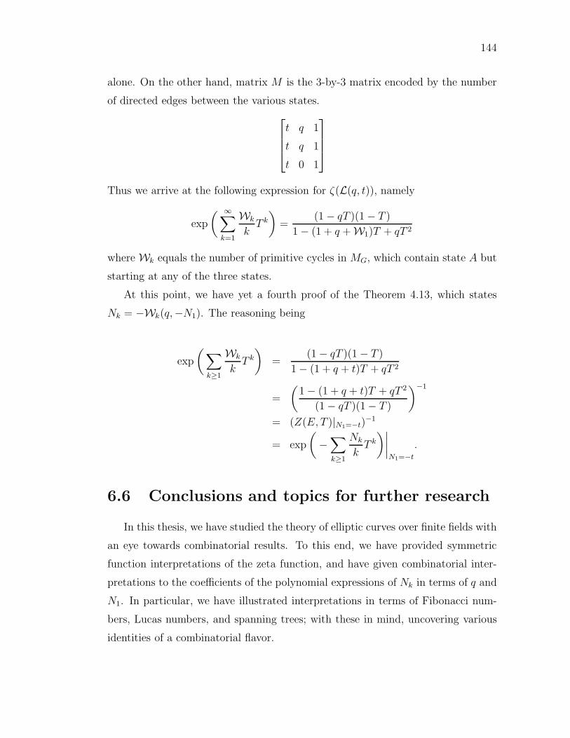
144

alone. On the other hand, matrix M is the 3-by-3 matrix encoded by the number

of directed edges between the various states.

t q 1

t q 1

t 0 1

Thus we arrive at the following expression for ζ(L(q, t)), namely

exp

( ∞∑

k=1

Wk

kT k

)

=(1− qT )(1− T )

1− (1 + q +W1)T + qT 2

where Wk equals the number of primitive cycles in MG, which contain state A but

starting at any of the three states.

At this point, we have yet a fourth proof of the Theorem 4.13, which states

Nk = −Wk(q,−N1). The reasoning being

exp

(

∑

k≥1

Wk

kT k

)

=(1− qT )(1− T )

1− (1 + q + t)T + qT 2

=

(

1− (1 + q + t)T + qT 2

(1− qT )(1− T )

)−1

= (Z(E, T )|N1=−t)−1

= exp

(

−∑

k≥1

Nk

kT k

)∣

∣

∣

∣

N1=−t

.

6.6 Conclusions and topics for further research

In this thesis, we have studied the theory of elliptic curves over finite fields with

an eye towards combinatorial results. To this end, we have provided symmetric

function interpretations of the zeta function, and have given combinatorial inter-

pretations to the coefficients of the polynomial expressions of Nk in terms of q and

N1. In particular, we have illustrated interpretations in terms of Fibonacci num-

bers, Lucas numbers, and spanning trees; with these in mind, uncovering various

identities of a combinatorial flavor.

145

As a bonus, as described in Chapter 6, the relationship between elliptic curves

and spanning trees appears even more pronounced than one would have guessed

from the motivation of Theorem 4.13. Not only do we have formal identities

relating the number of spanning trees of wheel graphs and number of points on

elliptic curves, but we also have connections between the corresponding group

structures of these two families of objects. The connections described here inspire

further exploration for connections between these two topics. In addition, future

research will consider more techniques from areas such as combinatorics on words

and dynamical system and use these to ask or answer questions about elliptic

curves.

In Chapter 2, we also discussed combinatorial aspects of algebraic curves in

general, using symmetric function theory for the general case. With such tech-

niques in mind, the study of higher genus curves such as hyperelliptic curves, or

other classes of abelian varieties will provide many other interesting topics for

exploration.

References

[BY06] Arthur T. Benjamin and Carl R. Yerger, Combinatorial interpretationsof spanning tree identities, Bull. Inst. Combin. Appl. 47 (2006), 37–42.

[Big99] N. L. Biggs, Chip-firing and the critical group of a graph, J. AlgebraicCombin. 9 (1999), no. 1, 25–45.

[BW] N. L. Biggs and P. Winkler, Chip-firing and the chromatic polynomial,CDAM Research Report Series, 97–03.

[Bom74] Enrico Bombieri, Counting points on curves over finite fields (d’apresS. A. Stepanov), Seminaire Bourbaki, 25eme annee (1972/1973), Exp.No. 430, Springer, Berlin, 1974, pp. 234–241. Lecture Notes in Math.,Vol. 383.

[BP86] F. T. Boesch and H. Prodinger, Spanning tree formulas and Chebyshevpolynomials, Graphs Combin. 2 (1986), no. 3, 191–200.

[BR90] Jean Berstel and Christophe Reutenauer, Zeta functions of formal lan-guages, Trans. Amer. Math. Soc. 321 (1990), no. 2, 533–546.

[BT51] H. D. Block and H. P. Thielman, Commutative polynomials, Quart. J.Math., Oxford Ser. (2) 2 (1951), 241–243.

[BE95] Peter Borwein and Tamas Erdelyi, Polynomials and polynomial inequal-ities, Graduate Texts in Mathematics, vol. 161, Springer-Verlag, NewYork, 1995.

[Cas91] J. W. S. Cassels, Lectures on elliptic curves, London Mathematical So-ciety Student Texts, vol. 24, Cambridge University Press, Cambridge,1991.

[CE02] Fan Chung and Robert B. Ellis, A chip-firing game and Dirichlet eigen-values, Discrete Math. 257 (2002), no. 2-3, 341–355, Kleitman andcombinatorics: a celebration (Cambridge, MA, 1999).

146

147

[Del74] Pierre Deligne, La conjecture de Weil. I, Inst. Hautes Etudes Sci. Publ.Math. (1974), no. 43, 273–307.

[DF91] David S. Dummit and Richard M. Foote, Abstract algebra, Prentice HallInc., Englewood Cliffs, NJ, 1991.

[Dwo60] Bernard Dwork, On the rationality of the zeta function of an algebraicvariety, Amer. J. Math. 82 (1960), 631–648.

[EI02] R.B. Ellis III, Chip-Firing Games with Dirichlet Eigenvalues and Dis-crete Greens Functions, Ph.D. thesis, UCSD, 2002.

[ER91] Omer Egecioglu and Jeffrey B. Remmel, Brick tabloids and the con-nection matrices between bases of symmetric functions, Discrete Appl.Math. 34 (1991), no. 1-3, 107–120, Combinatorics and theoretical com-puter science (Washington, DC, 1989).

[Fre01] Gerhard Frey, Applications of arithmetical geometry to cryptographicconstructions, Finite fields and applications (Augsburg, 1999), Springer,Berlin, 2001, pp. 128–161.

[Ful89] William Fulton, Algebraic curves, Advanced Book Classics, Addison-Wesley Publishing Company Advanced Book Program, Redwood City,CA, 1989, An introduction to algebraic geometry, Notes written withthe collaboration of Richard Weiss, Reprint of 1969 original.

[Gan] Wee Tak Gan, Lecture notes, UCSD 2005.

[GM] Adriano Garsia and Gregg Musiker, Basics on hyperelliptic curves overfinite fields, Mongraphies du LaCIM, To appear.

[Har77] Robin Hartshorne, Algebraic geometry, Springer-Verlag, New York,1977, Graduate Texts in Mathematics, No. 52.

[Has34] H. Hasse, Abstrakte Begrundung der komplexen Multiplikation und Rie-mannsche Vermutung in Funktionenkorpern, Abh. Math. Sem. Univ.Hamburg 10 (1934), 250–263.

[Hus04] Dale Husemoller, Elliptic curves, second ed., Graduate Texts in Math-ematics, vol. 111, Springer-Verlag, New York, 2004, With appendicesby Otto Forster, Ruth Lawrence and Stefan Theisen.

[IPS00] Mourad E. H. Ismail, Helmut Prodinger, and Dennis Stanton, Schur’sdeterminants and partition theorems, Sem. Lothar. Combin. 44 (2000),Art. B44a, 10 pp. (electronic).

148

[JNR03] Brian Jacobson, Andrew Niedermaier, and Victor Reiner, Criticalgroups for complete multipartite graphs and Cartesian products of com-plete graphs, J. Graph Theory 44 (2003), no. 3, 231–250.

[Lan78] Serge Lang, Elliptic curves: Diophantine analysis, Grundlehren derMathematischen Wissenschaften [Fundamental Principles of Mathe-matical Sciences], vol. 231, Springer-Verlag, Berlin, 1978.

[Lan82] , Introduction to algebraic and abelian functions, second ed.,Graduate Texts in Mathematics, vol. 89, Springer-Verlag, New York,1982.

[Len96] H. W. Lenstra, Jr., Complex multiplication structure of elliptic curves,J. Number Theory 56 (1996), no. 2, 227–241.

[Lor00] Dino Lorenzini, Arithmetical properties of Laplacians of graphs, Linearand Multilinear Algebra 47 (2000), no. 4, 281–306.

[LP01] Matthieu Latapy and Ha Duong Phan, The lattice structure of chipfiring games and related models, Phys. D 155 (2001), no. 1-2, 69–82.

[LWW04] Nicholas A. Loehr, Gregory S. Warrington, and Herbert S. Wilf, Thecombinatorics of a three-line circulant determinant, Israel J. Math. 143(2004), 141–156.

[Mac60] Percy A. MacMahon, Combinatory analysis, Two volumes (bound asone), Chelsea Publishing Co., New York, 1960.

[Mac95] I. G. Macdonald, Symmetric functions and Hall polynomials, seconded., Oxford Mathematical Monographs, The Clarendon Press OxfordUniversity Press, New York, 1995, With contributions by A. Zelevinsky,Oxford Science Publications.

[Max06] Molly Maxwell, Enumerating bases of self-dual matroids, 2006.

[Mer05] Criel Merino, The chip-firing game, Discrete Math. 302 (2005), no. 1-3,188–210.

[Mil06] J. S. Milne, Elliptic curves, BookSurge Publishers, Charleston, SC,2006.

[Mor91] Carlos Moreno, Algebraic curves over finite fields, Cambridge Tracts inMathematics, vol. 97, Cambridge University Press, Cambridge, 1991.

[MOV93] Alfred J. Menezes, Tatsuaki Okamoto, and Scott A. Vanstone, Reducingelliptic curve logarithms to logarithms in a finite field, IEEE Trans.Inform. Theory 39 (1993), no. 5, 1639–1646.

149

[MP07] G. Musiker and J. Propp, Combinatorial Interpretations for Rank-TwoCluster Algebras of Affine Type, the electronic journal of combinatorics14 (2007), no. R15, 1.

[Mye71] B. Myers, Number of spanning trees in a wheel, Circuits and Systems,IEEE Transactions on [legacy, pre-1988] 18 (1971), no. 2, 280–282.

[Pro] Jim Propp, Somos sequence website,http://www.math.wisc.edu/~propp/somos.html.

[Reu95] Christophe Reutenauer, On symmetric functions related to Witt vectorsand the free Lie algebra, Adv. Math. 110 (1995), no. 2, 234–246.

[Reu97] , N-rationality of zeta functions, Adv. in Appl. Math. 18 (1997),no. 1, 1–17.

[Sil92] Joseph H. Silverman, The arithmetic of elliptic curves, Graduate Textsin Mathematics, vol. 106, Springer-Verlag, New York, 1992, Correctedreprint of the 1986 original.

[Slo] N.J.A. Sloane, The on-line encyclopedia of integer sequences,http://www.research.att.com/∼ njas/sequences/index.html.

[Sta73] H. M. Stark, On the Riemann hypothesis in hyperelliptic function fields,Analytic number theory (Proc. Sympos. Pure Math., Vol. XXIV, St.Louis Univ., St. Louis, Mo., 1972), Amer. Math. Soc., Providence, R.I.,1973, pp. 285–302.

[Sta97] Richard P. Stanley, Enumerative combinatorics. Vol. 1, CambridgeStudies in Advanced Mathematics, vol. 49, Cambridge University Press,Cambridge, 1997, With a foreword by Gian-Carlo Rota, Correctedreprint of the 1986 original.

[Sta99] Richard P. Stanley, Enumerative combinatorics. Vol. 2, CambridgeStudies in Advanced Mathematics, vol. 62, Cambridge University Press,Cambridge, 1999, With a foreword by Gian-Carlo Rota and appendix1 by Sergey Fomin.

[Swa] C. Swart, Elliptic curves and related sequences, Ph.D. thesis, PhD The-sis, Royal Holloway and Bedford New College, University of London,2003.

[VDPS06] A.J. Van Der Poorten and C.S. Swart, Recurrence relations for ellipticsequences: every Somos 4 is a Somosk, Bulletin of the London Mathe-matical Society 38 (2006), no. 04, 546–554.

150

[Wag00] D.G. Wagner, The critical group of a directed graph,arXiv:math.C0/0010241 (2000).

[War48] Morgan Ward, Memoir on elliptic divisibility sequences, Amer. J. Math.70 (1948), 31–74.

[Was03] Lawrence C. Washington, Elliptic curves, Discrete Mathematics and itsApplications (Boca Raton), Chapman & Hall/CRC, Boca Raton, FL,2003, Number theory and cryptography.

[Wei48] Andre Weil, Sur les courbes algebriques et les varietes qui s’endeduisent, Actualites Sci. Ind., no. 1041 = Publ. Inst. Math. Univ.Strasbourg 7 (1945), Hermann et Cie., Paris, 1948.

[Wit01] Christian Wittmann, Group structure of elliptic curves over finite fields,J. Number Theory 88 (2001), no. 2, 335–344.

[Zel07] A. Zelevinsky, Semicanonical basis generators of the cluster algebra oftype, the electronic journal of combinatorics 14 (2007), no. 4, 1.

[ZYG05] Yuanping Zhang, Xuerong Yong, and Mordecai J. Golin, Chebyshevpolynomials and spanning tree formulas for circulant and related graphs,Discrete Math. 298 (2005), no. 1-3, 334–364.