A COINTEGRATION ANALYSIS OF HOUSEPRICE FORMATION IN THE HELSINKI

METROPOLITAN AREA

Lauri Saarinen

University of HelsinkiFaculty of Social SciencesEconomicsMaster’s thesisNovember 2013

Tiedekunta/Osasto – Fakultet/Sektion – Faculty

Faculty of Social Sciences

Laitos – Institution – Department

Department of Political and Economic Studies

Tekijä – Författare – Author

Lauri Saarinen

Työn nimi – Arbetets titel – Title

A cointegration analysis of house price formation in the Helsinki metropolitan area

Oppiaine – Läroämne – Subject

Economics

Työn laji – Arbetets art – Level

Master’s thesis

Aika – Datum – Month and year

November 2013

Sivumäärä – Sidoantal – Number of pages

57

Tiivistelmä – Referat – Abstract The thesis examines house price formation in the Helsinki metropolitan area. Especially the price appreciation following financial liberalisation of the late 1980’s and the subsequent price decline of the early 1990’s recession mark the development of house prices. During the 2000’s house prices have increased rapidly with the exception of the slump during the financial crisis. This thesis focuses on explaining the aforementioned development with emphasis on the long-run aspect in both theoretical and empirical examinations. The primary goal is in studying long-run interdependence between house prices and fundamental determinants mentioned in theoretical and empirical literature. Based on the achieved results it is possible to draw conclusions on the sustainability of the price level as well as study the effects of various fundamentals on the metropolitan area price level. The thesis is separated into a theoretical and an empirical section which makes use of econometric methods in modelling house prices. The long-run relationship between house prices and selected fundamental variables is examined using cointegration analysis. The fundamentals and house prices are modelled in a vector error correction framework central to cointegration analysis. Alongside house prices, household disposable income, mortgage interest rates, metropolitan area total net migration and the stock of housing loans describing household indebtedness are introduced into the system. The quarterly data are compiled from Statistics Finland and Bank of Finland databases for the time period 1983–2012. The central result of the thesis is a long-run equilibrium model between house prices and the fundamental determinants. The model is found to work satisfactorily as the results accord with theory and the results are statistically significant. In addition, the results are in line with previous empirical studies conducted in Finland. Furthermore it is discovered that mortgage interest rates, household indebtedness and migration patterns have been notable factors in determining house prices, especially towards the end of the examination period. The achieved results on short-run dynamics also provide support to the estimated long-run model. A key finding considering the short-run dynamics is the sluggish adjustment of house prices towards their long-run level. Based on the results of this thesis, house prices in the Helsinki metropolitan area have exceeded the estimated long-run equilibrium price level for a prolonged period. This phenomenon can be explained by demand side factors including high net migration to the region as well as low mortgage rates encouraging mortgage lending. On the other hand, inelastic supply and scarcity of land specific to urban areas restrain the rapid unravelling of excess demand in the housing market. It is thus possible, that in the future house prices will adjust downward toward their long-run equilibrium level.

Avainsanat – Nyckelord – Keywords

House prices, cointegration, error correction

Tiedekunta/Osasto – Fakultet/Sektion – Faculty

Valtiotieteellinen tiedekunta

Laitos – Institution – Department

Politiikan ja talouden tutkimuksen laitos

Tekijä – Författare – Author

Lauri Saarinen

Työn nimi – Arbetets titel – Title

Yhteisintegroituvuusanalyysi asuntojen hintojen muodostumisesta pääkaupunkiseudulla

Oppiaine – Läroämne – Subject

Taloustiede

Työn laji – Arbetets art – Level

Pro gradu -tutkielma

Aika – Datum – Month and year

Marraskuu 2013

Sivumäärä – Sidoantal – Number of pages

57

Tiivistelmä – Referat – Abstract Pro gradu -tutkielma tarkastelee asuntojen hintojen muodostumista pääkaupunkiseudulla. Erityisesti Suomen rahoitusmarkkinoiden vapautumista seurannut hintatason nousu 1980-luvun lopulla sekä 1990-luvun alun laman aikainen hintojen lasku leimaavat hintakehitystä. Asuntojen hinnat ovat nousseet vauhdikkaasti 2000-luvun puolella, lukuun ottamatta finanssikriisin aikaista hintatason notkahdusta. Tämä tutkielma keskittyy selittämään kuvattua kehitystä keskittyen pitkän aikavälin tarkasteluihin niin asuntojen hintojen muodostumisen teorian kuin empiiristen tarkastelujen osalta. Työn ensisijainen tavoite on tutkia pitkän aikavälin riippuvuussuhteita asuntojen hintojen sekä teorian mukaisten fundamentaalisten muuttujien välillä. Saatujen tulosten avulla on mahdollista tehdä johtopäätöksiä hintatason kestävyydestä sekä eri tekijöiden vaikutuksista pääkaupunkiseudun asuntojen yleiseen hintatasoon. Tutkielma jakaantuu teoreettiseen tarkasteluun sekä empiiriseen osioon, joka hyödyntää ekonometrisiä menetelmiä asuntojen hintojen mallintamisessa. Tutkimuksessa tarkastellaan asuntohintojen ja muiden muuttujien välistä pitkän aikavälin tasapainoriippuvuutta eli niin sanottua yhteisintegroituvuutta. Keskeisenä ekonometrisenä menetelmänä tutkimuksessa muotoillaan ja estimoidaan asuntojen hintojen sekä muiden muuttujien välistä käyttäytymistä kuvaava vektorivirheenkorjausmalli. Asuntojen hintojen ohella muita analysoitavia muuttujia ovat kotitalouksien käytettävissä olevat tulot, asuntoluottojen korot, pääkaupunkiseudun kokonaisnettomuutto sekä kotitalouksien velkaantumista kuvaava asuntoluottojen kanta. Käytetty aineisto on koottu Tilastokeskuksen ja Suomen Pankin aineistosta ja sisältää neljännesvuosittaiset aikasarjat edellä mainituista muuttujista aikavälillä 1983–2012. Tärkeimpänä tuloksena saadaan pitkän aikavälin riippuvuussuhde pääkaupunkiseudun asuntojen hintojen ja edellä mainittujen muuttujien välille. Mallin havaitaan toimivan hyvin, sillä tulokset ovat teorian mukaisia ja tilastollisesti merkitseviä. Tulokset ovat myös pääpiirteittäin linjassa aiempien Suomessa tehtyjen tutkimusten kanssa. Jatkotarkastelussa havaitaan erityisesti asuntoluottojen korkojen, asuntoluottokannan sekä muuttoliikkeen olleen merkitseviä tekijöitä hintojen määräytymisessä etenkin tutkimusperiodin loppuvaiheessa. Lyhyen aikavälin hintadynamiikkaa koskevat tulokset tukevat osaltaan estimoitua pitkän aikavälin tasapainorelaatiota. Tärkeimpänä lyhyen aikavälin dynamiikkaa koskevana löydöksenä voidaan pitää havaittua asuntojen hintojen hidasta sopeutumista estimoidun pitkän aikavälin mallin mukaiseen tasoon. Tulosten perusteella pääkaupunkiseudun asuntojen hinnat ovat olleet tutkielman kirjoitushetkellä jo pitkään estimoidun pitkän aikavälin riippuvuussuhteen mukaista tasoa korkeammalla. Ilmiön voidaan todeta johtuvan kysyntäpuolen tekijöistä, joihin lukeutuvat vahva muuttoliike seudulle sekä luotonottoon kannustava alhainen korkotaso. Toisaalta kaupunkialueille ominainen pula tonttimaasta yhdistettynä tuotannon jäykkyyteen estää liikakysyntätilanteen nopean purkautumisen. On näin ollen mahdollista, että tulevaisuudessa asuntojen hinnat sopeutuvat alaspäin kohti pitkän aikavälin tasapainoa.

Avainsanat – Nyckelord – Keywords

Asuntojen hinnat, yhteisintegroituvuus, virheenkorjausmalli

Contents

1 Introduction 1

2 Introduction to the housing markets 32.1 Housing market characteristics . . . . . . . . . . . . . . . . . . . . 32.2 Housing markets and the macroeconomy . . . . . . . . . . . . . . 52.3 The Finnish and the Helsinki Metropolitan Area

housing market developments . . . . . . . . . . . . . . . . . . . . 62.4 Recent demographic developments . . . . . . . . . . . . . . . . . . 9

3 Theoretical models of house price formation 153.1 The asset market approach . . . . . . . . . . . . . . . . . . . . . . 153.2 The present value approach . . . . . . . . . . . . . . . . . . . . . 19

4 Studies on house price dynamics 214.1 House prices and fundamentals . . . . . . . . . . . . . . . . . . . 224.2 Short-run dynamics . . . . . . . . . . . . . . . . . . . . . . . . . . 29

5 Research Methodology 315.1 Cointegration . . . . . . . . . . . . . . . . . . . . . . . . . . . . . 315.2 Deterministic terms . . . . . . . . . . . . . . . . . . . . . . . . . . 335.3 Testing for cointegration . . . . . . . . . . . . . . . . . . . . . . . 36

6 Data 386.1 House prices . . . . . . . . . . . . . . . . . . . . . . . . . . . . . . 386.2 Income . . . . . . . . . . . . . . . . . . . . . . . . . . . . . . . . . 396.3 Household indebtedness . . . . . . . . . . . . . . . . . . . . . . . 396.4 Interest rates . . . . . . . . . . . . . . . . . . . . . . . . . . . . . 416.5 Demography . . . . . . . . . . . . . . . . . . . . . . . . . . . . . . 41

7 Econometric Analysis 43

8 Conclusions 49

9 Appendix 58

1 Introduction

Over the past three decades price fluctuations in the Finnish housing markets

have been very significant. In the Helsinki Metropolitan Area (HMA)1 real house

prices rose by 66 percent between the final quarter of 1986 and the first quarter

of 1989. In the housing market literature this housing price bubble has been

associated with the deregulation of Finnish financial markets which eased bank

lending constraints and lead to higher household debt. Low real interest rates

and favourable tax conditions for owner occupied housing also contributed to ris-

ing house prices. Similarly, a rapid decline in the housing markets was recorded

from the peak of 1989 to the final quarter of 1992, as real prices plummeted 57

percent. This collapse has in turn, been associated to the severe recession that

hit the Finnish economy in the early 1990’s which prolonged the stagnation in

the housing markets. Large scale unemployment combined with tightened bank

lending and rising real interest rates as well as tax reforms had the effect of push-

ing down housing demand and prices. Despite these fluctuations real house prices

in the HMA have risen by 99 percent between 1983 and the end of 2012.

This thesis is an attempt on explaining these housing price patterns in the period

1983 to 2012 by means of econometric analysis. As housing markets are highly

regional in nature, the analysis is restricted to the HMA. For example, Oikarinen

(2007, 12) notes that regional housing price development in Finland has diverged

extensively since the early 1990’s due to increased migration from peripheral to

central areas. Previous studies have determined a wide range of fundamental

economic factors underlying house price fluctuations in the long-run. These fun-

damental factors include household incomes, bank lending, constructions costs,

demographics, real interest rates and tax treatment of owner-occupied housing

1The Helsinki Metropolitan Area consists of Espoo, Helsinki, Kauniainen and Vantaa.

1

to mention a few. In this thesis, the main focus is on analysing the long-run de-

terminants of housing prices and on constructing a long-run equilibrium model.

The model will also be used to the analysis of short-run dynamics and can be

used to draw conclusions on the sustainability of recent house price developments

in the HMA.

The thesis will begin with a brief introduction to the characteristics of the markets

for housing and the significance of housing markets to the macroeconomy. Specific

characteristics and recent history of the Finnish and the HMA housing markets

are also presented. The section finishes with a look into demographic changes

which have affected the housing markets and trends in housing production. In

the second section theoretical models of house price formation are reviewed. The

section ends with a remark on empirical application. The third section surveys

recent housing market studies focusing especially on the estimated long-run rela-

tionship between house prices and fundamentals. Short-run price dynamics are

also reviewed. The next section introduces the research methodology. Section five

presents and discusses the data. The empirical results are presented and discussed

in section six. The final section summarises the main findings and concludes.

2

2 Introduction to the housing markets

This section begins with an introduction to the housing market and more par-

ticularly on what separates the housing market from markets for other goods

and services. The macroeconomic implications of the housing markets will be

discussed right after. Next, the key developments and institutional changes of

HMA and Finnish housing markets from the previous three decades are covered.

The section is finished with a brief look into the metropolitan area demographic

changes which have undoubtedly influenced the HMA housing markets.

2.1 Housing market characteristics

The operation of housing markets differs significantly from other markets for

goods and services. Housing is in itself consumed by households as any other

good or service, but notably dwellings can simultaneously form a major part of

household wealth. Laakso & Loikkanen (2004) review some of the characteris-

tics of the housing markets. First of all, housing is a necessity and very often

fixed to a location. This obviously does not imply the ownership of a dwelling

as renting is an option. Housing is also a particularly expensive good. The mar-

ket price of a medium sized dwelling is approximately fourfold the income of an

average household in Finland (Laakso & Loikkanen 2004, 251). Third, housing

is a heterogeneous good as a particular dwelling is a combination of structural,

quantitative and qualitative characteristics. For example, the surrounding envi-

ronment is of importance when the choice of dwelling is made. In addition, it is

not only the dwellings that are heterogeneous but also the households demanding

housing services vary in their characteristics, income and preferences.

3

Another characteristic of the housing markets are high transaction costs related

to search, migration, taxation and other costs. Because of these high transac-

tion costs, households move from a dwelling to another relatively rarely. High

informational asymmetry is also a feature of the housing market. The seller is

presumably more aware of the true characteristics of the dwelling than the buyer.

Potential buyers have to evaluate the market value of a particular dwelling with

respect to sales made in the nearby area which poses difficulties due to the het-

erogeneity of housing.

As noted above, households have a choice when consuming housing services: typ-

ically the choice is between owner-occupied and market rental dwellings. In both

cases the household occupying the dwelling consumes the housing service. How-

ever, in the case of owner-occupancy, the dwelling forms a part of the residents’

stock of wealth. The household then receives return from ownership and bears

costs of housing and risk from possible future price and cost fluctuations. In

case of rental dwellings, the household simply receives a housing service and pays

compensation to the owner in the form of rent. The owner carries risk and other

costs as in the case of owner-occupied housing.

Finally, housing is a particularly long-term consumption good. The planning and

construction period of new dwellings is approximately two years at the shortest.

In addition, the production of new dwellings is low compared to the existing

stock of dwellings, varying between 1-3 % per annum (Laakso & Loikkanen 2004,

252). This implies that a large portion of the housing supply consists of existing

dwellings, further implying that households occupy the housing markets as both

buyers and sellers. Thus, housing supply is inelastic in nature and house prices

may be significantly autocorrelated at least in the short to medium run. As some

4

of the above suggests, the housing markets are of macroeconomic importance.

The necessity of housing and the high cost of housing consumption alone cause

housing markets to affect the whole economy.

2.2 Housing markets and the macroeconomy

Oikarinen (2007) reviews key interdependencies of the housing market and the

macroeconomy. First, for the reason that housing is an expensive good and

dwellings comprise the majority of many households’ wealth, changes in house

prices have major implications for household consumption. For example, in 2005

approximately 29 % of Finland’s national wealth was tied in residential buildings.

Altogether all buildings and constructs accounted for nearly 60 % of the national

wealth (Niemi & Sandstrom 2007). Benjamin et al. (2004) study the high con-

centration of household wealth in housing rather than in financial assets in the

United States. They find that the marginal propensity to consume from housing

wealth exceeds that for financial assets. Case, Quigley & Shiller (2001) find for

their international sample that propensity to consume from housing wealth varies

between 11 and 17 cents per dollar of wealth for each additional dollar of wealth,

whereas the corresponding figures for financial wealth are between zero and two

cents. Thus, fluctuations in house prices and housing wealth have significant ef-

fects on total consumption.

Second, falling housing price level has a negative impact on the housing con-

struction, which in turns has a negative impact on output and employment.

Third, housing price developments have considerable effects on the financial sec-

tor. There is a clear link between house prices and bank lending as banks relax

lending constraints when house prices are high. Similarly, a dip in housing prices

causes losses on mortgage lenders which can cause a negative shock for the fi-

5

nancial system. Goodhart & Hoffman (2007) note that houses are often used as

collateral for loans and thus a large share of financial sector assets are tied to

housing values. Therefore housing price fluctuations can have major impacts on

economic activity and the soundness of the financial sector as was shown in the

event of the financial crisis of 2007-2009.

2.3 The Finnish and the Helsinki Metropolitan Area

housing market developments

In 2012 the total Finnish stock of housing was approximately 2,556,000 dwellings.2

Owner-occupied housing accounted for about 65 % of the stock of dwellings.

Rental dwellings accounted for 30 %. About 1.4 % consisted of right of oc-

cupancy dwellings which is a specific tenure status introduced to the Finnish

housing markets in the early 1990’s to promote the supply of reasonably priced

dwellings. According to Oikarinen (2007, 57) institutional investors (inc. the

public sector) own approximately one half of the stock of rental dwellings. In

the HMA, the composition of the housing stock differs from the national stock.

In 2011, owner-occupied dwellings accounted for 52.6 %, rental dwellings for 42

% and right of occupancy dwellings for 3 % of total housing stock in the HMA.

The share of rental dwellings of the total stock decreased until the early 1990’s.

After a brief period of increase, the share of rental dwellings has further decreased

from the late 1990’s onward (Laakso & Loikkanen 2004, 248). Nevertheless, the

share of rental dwellings compared to owner-occupancy differs notably between

the HMA and the rest of the country. In addition, the share of multi-storey

housing companies of the total stock is higher in the HMA than in the rest of the

country.

2Source: Statistics Finland (a)

6

0

20

40

60

80

100

120

140

1983 1986 1989 1992 1995 1998 2001 2004 2007 2010

20

05

= 1

00

HMA

Finland

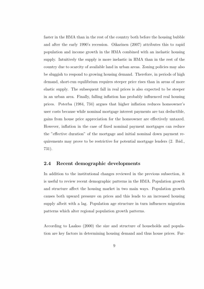
Figure 1: Real house prices in the HMA and in Finland 1983Q1-2012Q4(Source: Statistics Finland)

Figure 1 depicts the development of real house prices in the HMA and in Finland

from 1983 onward. The indices describe the evolution of the price of old dwellings

from 1983 to present.3 The two years of relatively stable real prices from 1984

to 1986 were followed by a period of rapid growth which lasted until the third

quarter of 1989. This period of rapid house price growth is generally associated

with the deregulation of the Finnish financial markets. Until the mid-1980’s bank

lending was strictly controlled along with foreign capital controls which lead to

credit rationing. In 1986 the Bank of Finland deregulated the banking system

and ceilings on lending rates were abolished. This improved the accessibility to

mortgages, especially as down payment ratios were relaxed. Deregulation rapidly

increased bank lending and caused a housing market boom.

The housing bubble burst at the end of 1989. Real prices declined until the end

3Section six presents a more precise description of the data

7

of 1992. In 1993 real housing prices were lower than in 1986 in the whole coun-

try. The fall in real prices was further deepened by the recession of the Finnish

economy in the early 1990’s. Kosonen (1997, 2) notes that falling or stagnating

household real income and mass unemployment further depressed the demand for

housing and accelerated price falls. As mentioned in the previous section, falling

house prices negatively impact new construction which reflected back into total

output. Increasing real interest rates also discouraged mortgage lending and re-

duced the demand for owner-occupied housing.

Furthermore, apart from strict regulation of the banking sector until the mid-

1980’s housing prices in Finland have been affected by rental controls and tax

deductibility of interest payments on mortgages. Real rents declined from early

1970’s to late 1980’s. Rent controls were abandoned in the period 1992-95 and

free market rents have increased since.4 The deductibility of interest payments

on mortgages in taxation implies a lower after-tax mortgage rate. This has the

effect of increasing demand for housing services. In Finland, interest payments

on mortgages were fully tax deductible up to 1974, then until 1992 the interest

payments were deductible in income taxation at marginal income tax rate. In

1993 the tax deductibility was further reduced. From then on interest payments

multiplied by the capital income tax rate have been deductible. Since 2012, the

deductible share has been lowered to 85% and in 2013 to 80% of interest pay-

ments. The tendency in tax treatment is clearly moving toward eliminating this

tax benefit encountered by mortgage lenders.

After the recession of the early 1990’s real prices have increased almost contin-

uously with the exception of the slowdown in 2008-09. Real prices have risen

4Removing rent controls should make owner-occupied housing more attractive and may havefed to house prices

8

faster in the HMA than in the rest of the country both before the housing bubble

and after the early 1990’s recession. Oikarinen (2007) attributes this to rapid

population and income growth in the HMA combined with an inelastic housing

supply. Intuitively the supply is more inelastic in HMA than in the rest of the

country due to scarcity of available land in urban areas. Zoning policies may also

be sluggish to respond to growing housing demand. Therefore, in periods of high

demand, short-run equilibrium requires steeper price rises than in areas of more

elastic supply. The subsequent fall in real prices is also expected to be steeper

in an urban area. Finally, falling inflation has probably influenced real housing

prices. Poterba (1984, 734) argues that higher inflation reduces homeowner’s

user costs because while nominal mortgage interest payments are tax deductible,

gains from house price appreciation for the homeowner are effectively untaxed.

However, inflation in the case of fixed nominal payment mortgages can reduce

the ”effective duration” of the mortgage and initial nominal down payment re-

quirements may prove to be restrictive for potential mortgage lenders (2. Ibid.,

731).

2.4 Recent demographic developments

In addition to the institutional changes reviewed in the previous subsection, it

is useful to review recent demographic patterns in the HMA. Population growth

and structure affect the housing market in two main ways. Population growth

causes both upward pressure on prices and this leads to an increased housing

supply albeit with a lag. Population age structure in turn influences migration

patterns which alter regional population growth patterns.

According to Laakso (2000) the size and structure of households and popula-

tion are key factors in determining housing demand and thus house prices. Fur-

9

thermore, migration also causes significantly greater fluctuations in the size and

structure of population at regional than at national level (Laakso 2000, 28). The

main reason for inter-regional variation in population development in Finland in

the recent decades has been migration. Mobility to the Helsinki region and other

major urban areas has increased from the countryside and smaller towns. In the

1980’s population growth in the Helsinki region accelerated due to employment

and income growth. Correspondingly the rural areas lost population to urban

areas (2. Ibid, 29).

-2000

0

2000

4000

6000

8000

10000

12000

14000

1980 1983 1986 1989 1992 1995 1998 2001 2004 2007 2010

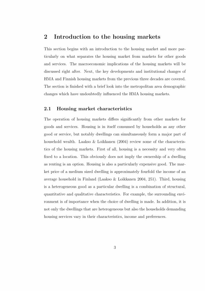
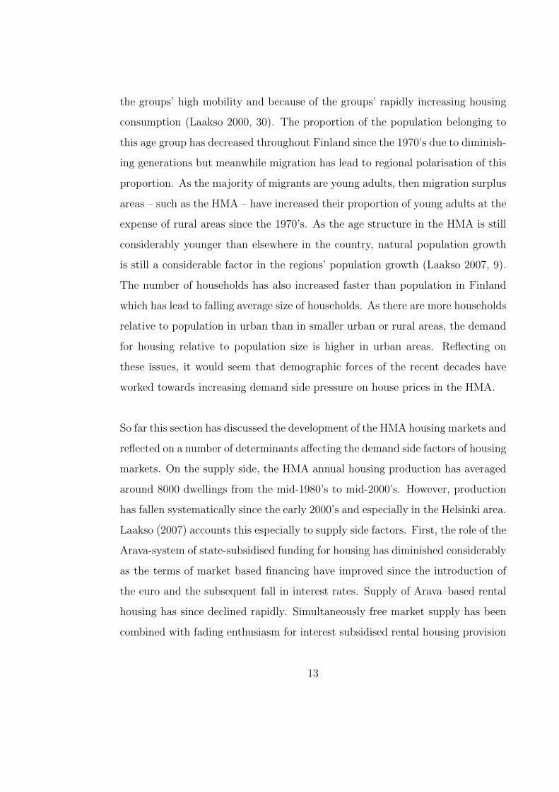
Figure 2: Annual net migration in HMA (Source: Statistics Finland)

The population trend changed in 1988-89, thus slowing down growth in Helsinki

region and decelerating the decline in rural areas. Migration from former Soviet

Union again shifted the falling population trend in the Helsinki region during

the recession era in 1991-93. Statistics show a notable increase in net migration

observed in most large urban areas in Finland from 1994 on (see Figure 2). This

is largely explained by the introduction of a new home municipality law which

came into effect beginning 1994, allowing students to be registered as residents

10

of the municipality in which they studied. Previously they had been registered

in the municipality of their parents’ home.

0

0,4

0,8

1,2

1,6

2

1980 1983 1986 1989 1992 1995 1998 2001 2004 2007 2010

%

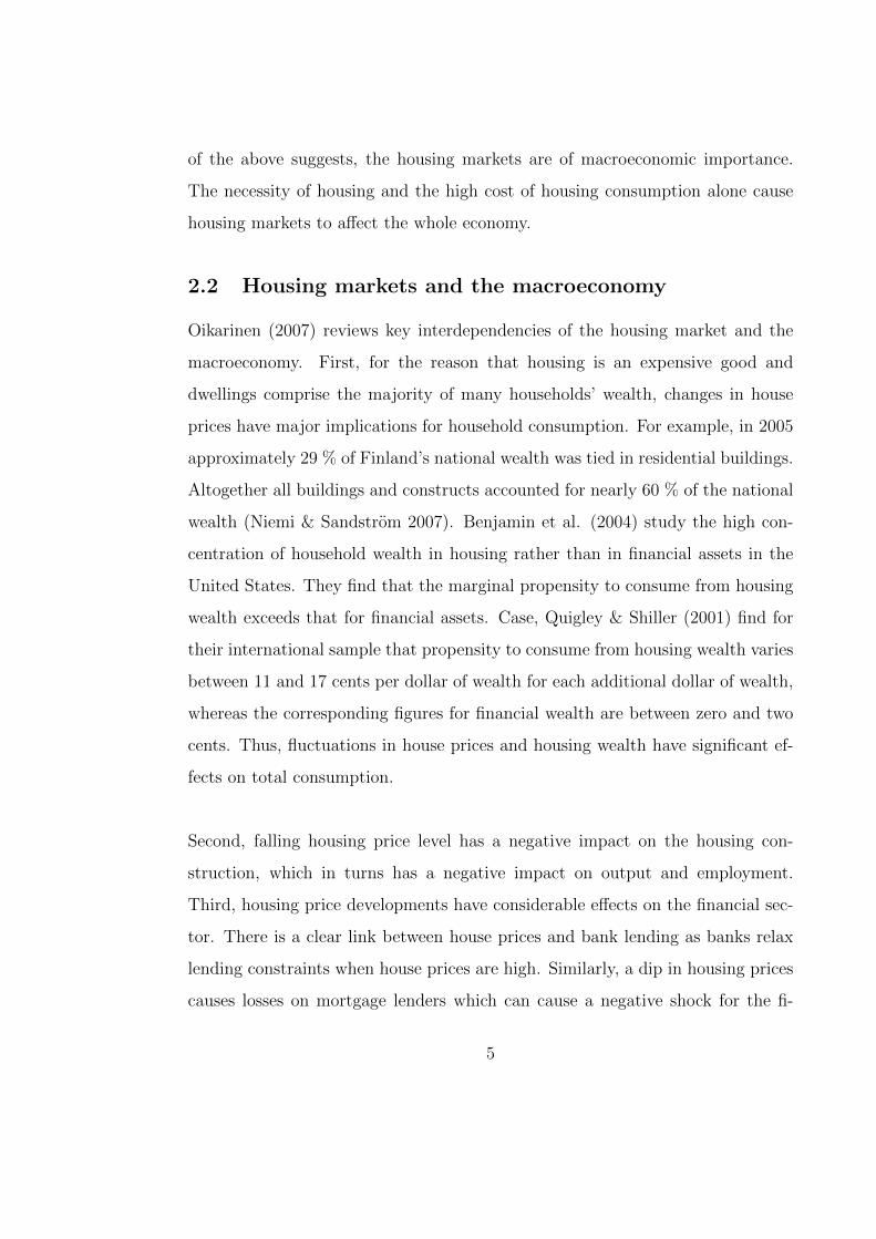
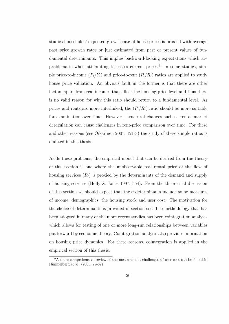
Figure 3: Annual population growth in the HMA (Source: Statistics Finland)

The population growth in HMA was fairly rapid in the late 1990’s and the first

years of the 2000’s. Figure 3 shows that growth slowed down between 2002 and

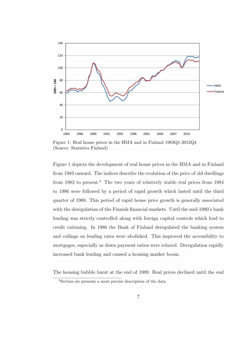
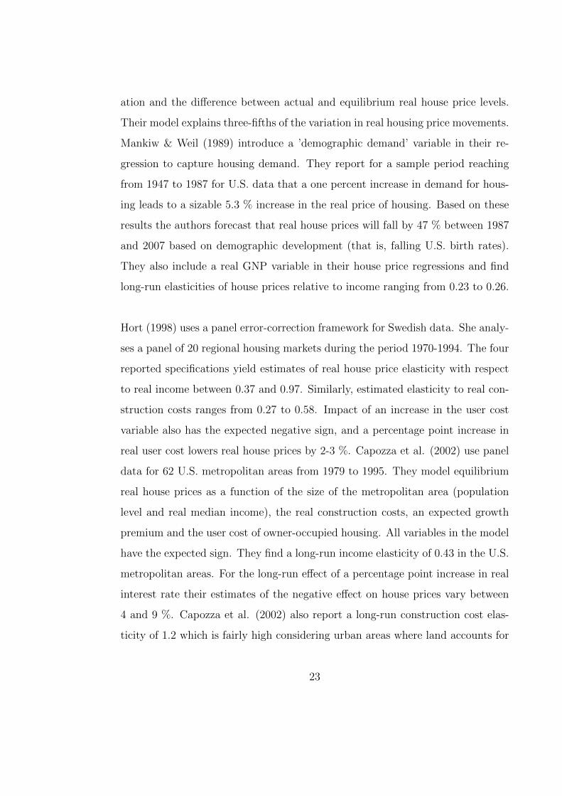
2004, but accelerated again in the years that followed. Figure 4 in turn shows

that the area was actually subject to negative net migration between 2003-05

when considering only Finnish citizens.5 Nivalainen & Vuori (2012, 162) recog-

nise two main reasons for the negative net migration of Finnish citizens to the

area in this period. Firstly, the depression in the technology sector in the early

2000’s tested areas with large concentration of employment in the sector such as

the HMA. Second, the decline in the rate of population growth for the period is

further explained by increased outward migration from the HMA to the so called

‘outer labour market area’ - or neighbouring municipalities - as a consequence

of declining interest rates which allowed especially families with children to con-

5Foreign citizens displayed in red, Finnish citizens in blue. Figure from Laakso (2007, 10)

11

struct affordable one-family housing in these areas. Nevertheless, the impact of

these migration patterns on Helsinki and the HMA was short lived as domestic

migration to the area increased post-2005 combined with the new coming of for-

eign in-migration beginning in 2005. In the 2000’s total net migration growth in

the Helsinki region has actually increasingly been down to foreign citizens and

less so down to Finnish citizens as is shown in figure 4.

Figure 4: Net migration of Finnish and non-Finnish citizens 1999-2006(Laakso 2007)

Laakso (2000) emphasizes the role of age structure of population as another key

determinant of housing demand alongside population size. Studies by Mankiw

& Weil (1989) for US data and Kuismanen et al. (1999) for HMA have shown

that housing consumption per capita with respect to age increases most rapidly

within the 20 to 29 year-old age group. In context of the housing markets, these

studies show the importance of this age group for the housing demand because of

12

the groups’ high mobility and because of the groups’ rapidly increasing housing

consumption (Laakso 2000, 30). The proportion of the population belonging to

this age group has decreased throughout Finland since the 1970’s due to diminish-

ing generations but meanwhile migration has lead to regional polarisation of this

proportion. As the majority of migrants are young adults, then migration surplus

areas – such as the HMA – have increased their proportion of young adults at the

expense of rural areas since the 1970’s. As the age structure in the HMA is still

considerably younger than elsewhere in the country, natural population growth

is still a considerable factor in the regions’ population growth (Laakso 2007, 9).

The number of households has also increased faster than population in Finland

which has lead to falling average size of households. As there are more households

relative to population in urban than in smaller urban or rural areas, the demand

for housing relative to population size is higher in urban areas. Reflecting on

these issues, it would seem that demographic forces of the recent decades have

worked towards increasing demand side pressure on house prices in the HMA.

So far this section has discussed the development of the HMA housing markets and

reflected on a number of determinants affecting the demand side factors of housing

markets. On the supply side, the HMA annual housing production has averaged

around 8000 dwellings from the mid-1980’s to mid-2000’s. However, production

has fallen systematically since the early 2000’s and especially in the Helsinki area.

Laakso (2007) accounts this especially to supply side factors. First, the role of the

Arava-system of state-subsidised funding for housing has diminished considerably

as the terms of market based financing have improved since the introduction of

the euro and the subsequent fall in interest rates. Supply of Arava–based rental

housing has since declined rapidly. Simultaneously free market supply has been

combined with fading enthusiasm for interest subsidised rental housing provision

13

by the municipalities, and these supply channels have been unable to compensate

for the supply reduction in the Helsinki area which has traditionally been the core

region of state supported housing supply. The availability of vacant lots for new

construction has also decreased since the 1990’s. Vacancy is further undermined

because possessors of privately owned sites hold on to land as increasing prices

of existing housing stock promote an optimal strategy of refraining from selling

in search of higher future returns. Interestingly, empirical literature on housing

price dynamics largely neglects the supply side of housing markets because sup-

ply side variables are hard to account for in empirical studies or provide little

additional explanatory power to empirical models. Potential supply side data

include a housing stock variable and real construction cost index, which is most

often used in empirical applications.6

6For additional information, see section 6 and Oikarinen (2007)

14

3 Theoretical models of house price formation

This section will review two theoretical models of house price formation which

have very similar implications for empirical estimation. As housing markets can

differ significantly regionally in terms of price level, growth and dynamics, it

should be noted that the following models are best thought of in a regional con-

text. A metropolitan area should be a suitable choice as dwellings in HMA can

be regarded as relatively close substitutes for each other. The section finishes

with a brief motivation for the methodological choice of section five.

3.1 The asset market approach

When attempting to determine a price for a dwelling, it is crucial to calculate

correctly the financial return associated with an owner-occupied property. Such

a calculation compares the value of living in that property for a year (”imputed

rent”, or what it would have cost to rent an equivalent property) with the lost

income that one would have received if the owner had invested the capital in an al-

ternative investment (”the opportunity cost of capital”). This comparison should

take into account differences in risk, tax benefits from owner-occupancy, property

taxes, maintenance expenses and any anticipated capital gains from owning the

house (Himmelberg et al. 2005, 74). This approach is known as the asset market

approach to owner-occupied housing introduced by Poterba (1984). The model

allows an economically justified way of assessing whether house prices are too

high or too low by comparison of user cost of owning a dwelling to renting. The

original article by Poterba (1984) considers only the price of house structures, but

the theory can be applied to situations were house price is an entity including

the structures and the land. The presentation follows Himmelberg et al. (2005).

15

The annual cost of homeownership or the ”imputed rent” is comprised of six com-

ponents which represent both costs and offsetting benefits to owner occupancy.

First, the homeowner incurs the cost of foregone interest that the homeowner

could have earned by investing in something other than a house. The one year

cost can be expressed as a multiplication of the price of a house Pt and the risk-

free interest rate rftt . Next, the one-year cost of property taxes is computed as

house price Pt times property tax rate ωt. Third, an offsetting benefit to owning,

namely the tax deductibility of mortgage interest and property tax is introduced.

This is estimated as the house price Pt times effective tax rate on income τt,

multiplied by estimated mortgage and property tax rates rmt and ωt, respectively.

In the Finnish case, τt should be viewed more broadly as tax benefit of mort-

gage payments, as the rules of tax deductibility of mortgage rates have changed

multiple times in the recent decades and interest on mortgage payments has not

been fully deductible after 1974 as discussed in section 2.3. The fourth term is δt

which reflects depreciation as a share of house value. The term can be thought of

as maintenance and repair costs required to retain a constant quality of dwelling

structures. Fifth, gt+1 is the expected capital gain or loss during a year and finally

Ptγt represents the additional risk premium to compensate homeowners for the

higher risk of owning versus renting. The resulting equation for the annual cost

of homeownership is

Cost of onwnership = Pt·rftt +Pt·ωt−Pt·τt·(rmt +ωt)+Pt·δt−Pt·gt+1+Pt·γt (3.1)

Oikarinen (2007, 28) notes that in Finland, property tax rate is not tax deductible

in the case of owner-occupancy, thus the equation can be simplified and assumed

that the term δt also includes the property tax. The equation becomes

Cost of onwnership = Pt · rftt − Pt · τt · rmt + Pt · δt − Pt · gt+1 + Pt · γt (3.2)

16

Housing market equilibrium requires that expected annual cost of ownership equal

the annual cost of renting. Thus, if annual ownership costs rise without corre-

sponding increases in rents, house prices must fall to attract potential buyers to

ownership rather than to rent. Obviously, the opposite applies in case ownership

costs fall without matching reductions in rental prices. This ”no arbitrage” con-

dition then implies that the sum of annual costs of housing must equal annual

rent. Equation (3.2) can be used to present this logic and to equate annual rent

Rt with the annual cost of ownership

Rt = Pt · ut (3.3)

where ut is the user cost of housing defined as

ut = rftt − τt · rmt + δt − gt+1 + γt

The user cost of housing is just the annual cost of ownership per dollar of house

value. Again, rearranging gives Pt/Rt = 1/ut, which states that the equilibrium

price-to-rent ratio should equal the inverse of user cost. Then, fluctuations in

the user cost lead to predictable changes in the price-to-rent ratio that reflect

changes in fundamental determinants. Comparing price-to-rent ratios over time

does not provide information about over- or undervaluation if user costs are not

taken into account in such an evaluation.

The role of inflation is key to house prices. As noted in the previous section, higher

inflation rates reduce homeowners’ user costs because while nominal mortgage

interest payments are tax deductible, the capital gains from house appreciation

are essentially untaxed (Poterba 1984, 734-5). This implies that an increase in

the rate of inflation, holding housing stock constant, increases real house prices.

However, inflation works in the opposite direction as well. Rising inflation raises

17

nominal interest rates, which implies a real rise in repayment of a usual annuity

mortgage in the early years of the loan. Tighter liquidity constraints in the be-

ginning of the lending period reduce demand for housing and depress house prices.

Real interest rate is also an important determinant for user cost of housing. A

lower real interest rate reduces the cost of a mortgage and simultaneously low-

ers the opportunity cost of residential investment. As mortgage interest is tax-

deductible and the opportunity cost of the equity in the house is taxable return,

a percentage point fall in real interest rate reduces the user cost by 1− τ (Him-

melberg et al. 2005, 76). The user cost formula also implies that a percentage

point decrease in real interest rates in a low interest rate environment causes a

larger percentage increase in real house prices than a similar percentage point

decrease would in a high real interest rate environment.7 As with real interest

rates, a higher income tax rate - when applicable - lowers the user cost of housing

as higher income taxation raises the tax-subsidy to owner-occupied housing. The

effect should be more pronounced for high tax rate households as their marginal

costs for housing also change the most (Poterba 1991, 152).

A metropolitan area where expected house price appreciation (expected inflation

and real expected appreciation rate of housing) is high has a lower user cost

than an area where expected appreciation is low. Himmelberg et al. (2005,

78) note that if the long-run supply of housing were perfectly elastic, then house

prices would be determined solely by construction costs and expected appreciation

would be determined by expected growth in real construction costs. However, the

long-run growth of house prices has historically exceeded growth in construction

costs. This suggests that land value is appreciating faster than the value of

7Empirical studies report an average sensitivity of house prices to interest rate changes, asit is difficult to account for different interest rate regimes.

18

structures. This is no surprise as especially in densely populated urban areas

land is in short supply, so demand growth capitalises into land prices.

3.2 The present value approach

The present value condition is very similar to the user cost view presented in the

previous section. The main idea behind the present value approach is that the

price of housing is the present discounted value of future net housing services.

Equation (3.3) of the previous subsection can be used to form an asset price

formula to describe the present value of housing.

Pt = Et

h∑t=1

[Rt − δt + τt · rmt

(1 + θt,t+η)η

]+ Et

[Ph

(1 + θ)h

](3.4)

where Pt is the price of a dwelling at time t and Et is the expectations operator.

θt,t+η denotes the required rate of return from time t to η and h is the length

of the planned investment horizon. The risk premium (γt) and the risk-free rate

(rftt ) are incorporated in θ. In this formulation δt and rmt refer to absolute values

of depreciation and mortgage payment.8 The present value formula as presented

in (3.4) consists of two components: the expected net rental capital income (im-

plicit rents) and expected house price appreciation. The analogy is the same as

in financial assets such as shares where total yield is composed of dividends and

price appreciation.

In empirical applications measurement problems arise with both methods as prob-

lems of evaluation of expected appreciation and rate of return still remain. It is

equally challenging to determine appropriate values for depreciation of a struc-

ture, not to mention the risk premium which also enters the formula. In many

8This manner of representation follows Oikarinen (2007)

19

studies households’ expected growth rate of house prices is proxied with average

past price growth rates or just estimated from past or present values of fun-

damental determinants. This implies backward-looking expectations which are

problematic when attempting to assess current prices.9 In some studies, sim-

ple price-to-income (Pt/Yt) and price-to-rent (Pt/Rt) ratios are applied to study

house price valuation. An obvious fault in the former is that there are other

factors apart from real incomes that affect the housing price level and thus there

is no valid reason for why this ratio should return to a fundamental level. As

prices and rents are more interlinked, the (Pt/Rt) ratio should be more suitable

for examination over time. However, structural changes such as rental market

deregulation can cause challenges in rent-price comparison over time. For these

and other reasons (see Oikarinen 2007, 121-3) the study of these simple ratios is

omitted in this thesis.

Aside these problems, the empirical model that can be derived from the theory

of this section is one where the unobservable real rental price of the flow of

housing services (Rt) is proxied by the determinants of the demand and supply

of housing services (Holly & Jones 1997, 554). From the theoretical discussion

of this section we should expect that these determinants include some measures

of income, demographics, the housing stock and user cost. The motivation for

the choice of determinants is provided in section six. The methodology that has

been adopted in many of the more recent studies has been cointegration analysis

which allows for testing of one or more long-run relationships between variables

put forward by economic theory. Cointegration analysis also provides information

on housing price dynamics. For these reasons, cointegration is applied in the

empirical section of this thesis.

9A more comprehensive review of the measurement challenges of user cost can be found inHimmelberg et al. (2005, 79-82)

20

4 Studies on house price dynamics

Most of the empirical research in the field of housing price dynamics concen-

trates on two major issues. First, most studies estimate a long-run equilibrium

price level. Often estimation results are compared with actual price dynamics

to draw conclusions on the possible under- or overvaluation of house prices in

specific periods. Secondly, studies analyse the short-run dynamic adjustment of

house prices after deviations from long-run equilibrium. In more recent studies

the methodology used is often cointegration analysis. Most studies acknowledge a

long-run relation towards which house prices adjust and find adjustment sluggish.

Similarly, there seems to be widespread consensus on the determinants of house

prices. However, there are large differences in empirical results largely due to

imperfect data and because housing markets have region-specific features. This

chapter reviews a selection of studies from the recent decades.

As discussed in the previous section, the user cost formula implies that the price

per unit of housing services is the user cost per dollar of house value multiplied by

the price level of houses. Then a change in the user cost per dollar of house value

should leave the cost of housing services unaffected and be offset by a proportion-

ate change in house prices. Thus, the elasticity of house price with respect to per

unit user cost should theoretically be equal to one. Then, building a regression

with house prices as a dependent variable and supply, user cost and possibly other

demand side variables as explanatory variables should provide estimates for the

price, income and other (long-run) elasticities. Since the supply side is harder to

measure, it is often omitted or replaced with an ’indirect’ measure of supply such

as construction cost index in empirical applications.

21

4.1 House prices and fundamentals

Most housing price studies find a statistically significant positive relationship be-

tween house prices and some measure of disposable income or GDP. Noting that

although income as such does not enter the theoretical models of the previous

section, it is almost always included in studies. Englund (2011, 43-44) argues that

since income is a major determinant of housing consumption and since supply

is constrained by scarcity of land, one would expect a close relationship between

household disposable income and house prices. Girouard et al. (2006) review

a large selection of studies conducted mainly in European countries or the U.S.

The panel studies and regional studies find elasticities of real house prices rel-

ative to real disposable income reaching from as low as 0.1 to 0.2 for Ireland

(McQuinn 2004) to 8.3 for Parisian markets (Bessone et al. 2005). Most of the

studies reviewed use an error-correction model to analyse price dynamics. Case

& Shiller (2003) use a rare methodology in the field of housing price studies as

they conduct a questionnaire survey for homebuyers in four U.S. metropolitan

areas in 2002. They find that for more than forty U.S. states income growth

alone explains almost all of the house price increase, however they find evidence

for the existence of a speculative bubble in some cities as well.

Some of the pioneering work on econometric house price modelling is introduced

in Hendry (1984). The ADL model specification is set up between average house

price to household income ratio, loan to income ratio, real income per house-

hold, inflation and after-tax interest rates. All coefficients have the expected

sign. Abraham & Hendershott (1996) employ a regression model to explain cross-

sectional annual variation in real house price movements in 30 U.S. cities over

the 1972-92 period. In the model real house appreciation is explained by changes

in the equilibrium price and adjustment dynamics including lagged real appreci-

22

ation and the difference between actual and equilibrium real house price levels.

Their model explains three-fifths of the variation in real housing price movements.

Mankiw & Weil (1989) introduce a ’demographic demand’ variable in their re-

gression to capture housing demand. They report for a sample period reaching

from 1947 to 1987 for U.S. data that a one percent increase in demand for hous-

ing leads to a sizable 5.3 % increase in the real price of housing. Based on these

results the authors forecast that real house prices will fall by 47 % between 1987

and 2007 based on demographic development (that is, falling U.S. birth rates).

They also include a real GNP variable in their house price regressions and find

long-run elasticities of house prices relative to income ranging from 0.23 to 0.26.

Hort (1998) uses a panel error-correction framework for Swedish data. She analy-

ses a panel of 20 regional housing markets during the period 1970-1994. The four

reported specifications yield estimates of real house price elasticity with respect

to real income between 0.37 and 0.97. Similarly, estimated elasticity to real con-

struction costs ranges from 0.27 to 0.58. Impact of an increase in the user cost

variable also has the expected negative sign, and a percentage point increase in

real user cost lowers real house prices by 2-3 %. Capozza et al. (2002) use panel

data for 62 U.S. metropolitan areas from 1979 to 1995. They model equilibrium

real house prices as a function of the size of the metropolitan area (population

level and real median income), the real construction costs, an expected growth

premium and the user cost of owner-occupied housing. All variables in the model

have the expected sign. They find a long-run income elasticity of 0.43 in the U.S.

metropolitan areas. For the long-run effect of a percentage point increase in real

interest rate their estimates of the negative effect on house prices vary between

4 and 9 %. Capozza et al. (2002) also report a long-run construction cost elas-

ticity of 1.2 which is fairly high considering urban areas where land accounts for

23

a sizeable portion of the house price.

Meese & Wallace (2003) survey house price dynamics in Paris using monthly

transaction-level data for the period 1986 to 1992. They estimate an error-

correction model with prices, a construction cost variable, the cost of capital,

employment and real income. They find a long-run income elasticity of 0.65 and

estimate that a percentage point increase in real after-tax interest rate leads to a

7 % fall in real house prices. Meese & Wallace (2003) find a long-run construction

cost elasticity of up to 6.5 which seems overly high. Moreover, the length of the

time period considered is very short for a housing market study. Holly & Jones

(1997) use a particularly long data set from 1939 to 1994 of annual observations

for the UK. They model real house prices with cointegration analysis using real

income, demography, interest rate, the housing stock and other variables and

find that the most important determinant of real house prices has been real in-

come. Hofmann (2004) uses a cointegrating VAR to analyse determinants of bank

credit to the private non-financial sector in 16 industrialised countries including

Finland. For Finland, Hofmann (2004) finds elasticity of real house prices with

respect to real GDP equal to 0.3. Similarly, for a credit-to-GDP ratio he finds an

elasticity of 0.6 with respect to prices. The estimated effect of a percentage point

change in real interest rates is a mere 0.5 % in real house prices, which is low com-

pared to other studies. Borowiecki (2009) uses a VAR framework to study Swiss

house prices between 1991-2007 and finds that real house prices are most sensitive

to changes in population and construction costs. A 1 % increase in population

aged 20 to 64 increases house prices by 2 %. An appreciation in construction

costs leads to roughly similar increase in house prices. GDP turned out to have

limited explanatory power which may be explained by the specification employed.

24

Hilbers et al. (2008) use a yearly panel of 16 European countries between 1985

and 2006 to estimate house price equations. They split the data into three groups

based on the rate of house price appreciation during the sample period. For the

’fast lane’ group they find that a percentage point increase in per capita output

raises house prices by 2.5 % which is three times more than for the slow growth

group. They report similar stronger effects for the fast lane group for a demo-

graphic variable, however the estimates have an unexpected negative effect and

are partially insignificant. Ganoulis & Giuliodori (2010) estimate a panel error-

correction model for a sample of European countries over the period 1970-2004.

In the long-run, the elasticity of real house prices with respect to real income is

found to lie between 0.9 and 1.5. Estimates of the semi-elasticity with respect

to interest rates range from -1.2 to -2.6. They also find that mortgage debt

enters the long-run relation albeit with a lower elasticity of approximately 0.3.

Ganoulis & Giuliodori (2010) split the sample to check for the effects of financial

liberalisation to find that the impulse effect of interest rates on house prices has

strengthened post-liberalisation and the effect of income and mortgage debt has

weakened.

Adams & Fuss (2010) construct a panel error-correction model for quarterly data

for 15 OECD countries between 1975-2007. They set up an economic activity

measure, which is composed of real money supply, real consumption, real indus-

trial production, real GDP and employment. In addition to the economic activity

variable, long-term interest rates and construction costs are added to the model.

The results indicate that the elasticity of house prices with respect to economic

activity is on average 0.34 for the panel group. For interest rates they find a

coefficient of -0.4 and the estimate for construction costs is 1.3.

25

Research of house price dynamics in the Finnish and HMA markets is quite lim-

ited. Kuismanen et al. (1999) use the approach introduced by Mankiw & Weil

(1989). They regress real housing prices for the HMA for the period 1962-1997 on

a demographic housing demand variable, a one period lagged real income variable

and others. They find that the long-run income elasticity of housing price level

is 0.81. Kosonen (1997) uses a methodology similar to Abraham & Hendershott

(1996) and uses quarterly data for Finland between 1979-1995. The ADL model

between real house prices, real disposable income and real after-tax interest rates

yields a long-run elasticity of real house prices with respect to income of approxi-

mately 1.4. Similarly, a one percentage point decrease in the real after-tax interest

rate increases real house prices by 9 % in the long-run equation. Barot & Takala

(1998) set up a model to find house prices and inflation cointegrated implying

stationary real house prices in Finland and Sweden. The authors admit that the

cointegrating relationship may seem puzzling, but find significant evidence.

Laakso (2000) employs annual panel data for 85 Finnish sub-regions from 1983 to

1997. The price model specification follows Abraham & Hendershott (1996). The

growth in equilibrium real housing prices in a specific region or city is a linear

function of the growth in real construction costs, real income per working age

adult, change in employment, vacancy rates and the change in real after-tax real

interest rates. Variables related to local demography are left out as they do not

add to the explanatory power when used with jobs and income. The estimation

results suggest that income and employment variables are positive and significant.

Real after-tax interest rate and the lagged vacancy rate have a strong negative

effect on real housing prices. The study also finds that basic trends of housing

markets were very similar in all regions in Finland during 1980’s and 1990’s.

Laakso (2000, 63) distinguishes a straight forward solution to this phenomenon:

26

“. . . the most crucial external effects on housing markets – changes in

interest rates, taxation rules, and income, employment and inflation

development - took place at national level and were transmitted to all

local housing markets approximately at the same time. Only years

after the depression, from 1997 on, there seem to have appeared clear

deviations between regions with respect to housing market develop-

ments: This is a consequence of recently increasing polarisation of

regional employment and population development.”

Oikarinen (2007) estimates a cointegrating long-run model between real house

prices, real aggregate income, a loan-to-GDP variable and real after-tax lending

rate using quarterly observations between 1975-2006 in the HMA. The real ag-

gregate income variable thus includes the effect of population growth on house

prices. The study finds that the combination of real disposable income growth and

population growth combined with loosening liquidity constraints have increased

long-run equilibrium housing prices in the area. Results indicate that a one per-

cent increase in real disposable income raises real house prices by approximately

0.4 %. Similarly, a percentage increase in the loan stock variable reflecting loosen-

ing liquidity constraints would yield a 0.5 % increase in house prices. Somewhat

surprisingly the real interest rate is not significant in the model. The model finds

no evidence for substantial overpricing in the HMA market in 2006. For Finnish

national-level data, Adams & Fuss (2010) find a 0.78 house price elasticity with

respect to their economic activity variable. Similarly to Oikarinen (2007) they

find the interest rate variable not significant for long-term house prices. A per-

centage increase in construction costs feeds a 0.93 % rise in house prices in the

long-run in their estimation.

To sum up evidence from these studies, there is strong evidence that house prices

27

are increasing functions of income, population growth and loosening credit con-

straints. Similarly, higher real after-tax interest rate which also tracks user cost

has a significant negative impact on real house prices in most studies. On aver-

age, the income elasticity of house prices is around one, though there is a lot of

variation in results. According to Englund (2011, 45) this implies that in order

to meet the growing housing demand, the housing stock would have to grow at

the same rate as income is growing in a society. Otherwise, house prices will have

to rise to guarantee a balance between demand and supply. Even though only a

few results for the Finnish markets were reviewed some thoughts can be weighed

in. It would seem that older studies like Kosonen (1997) and Laakso (2000) find

stronger effects of income and interest rate variables on real house prices than the

more recent studies by Oikarinen (2007) and Adams & Fuss (2010). The observa-

tion of long-run de-linking of house prices and income seems somewhat surprising

as international studies find no evidence of changes in the long-run relation over

time.10 The results on the semi-elasticities of house prices with respect to real

interest rates seem equally confusing. As argued in the previous section, Himmel-

berg et al. (2005) suggested stronger effects of real interest rates on real house

prices in a low interest rate environment. However, the aforementioned recent

studies on Finnish and the HMA housing markets find very moderate effects of

interest rates on house prices despite the fact that the interest rate environment

is notably lower when compared to the data period considered in the older studies.

10See for example Ganoulis & Giuliodori (2010) who split the sample period to pre- and postfinancial liberalisation periods.

28

4.2 Short-run dynamics

Short-run price movements can deviate from the long-run trends for at least three

reasons: supply inertia, expectations formation and credit constraints. Therefore,

we should expect cyclicality of house prices in the short to medium-run, but in

the long-run housing supply should lead prices towards an equilibrium level de-

termined by fundamentals (Englund 2011, 49). This reasoning is behind the use

of the error-correction models in a majority of studies. Some results concerning

adjustment dynamics are reviewed below. A connective factor to almost all the

studies is that they find adjustment in the housing markets sluggish.

Holly & Jones (1997) find that the dynamic adjustment of house prices has been

asymmetric depending on whether house prices are above or below their long-

run path: adjustment to long-run equilibrium is faster, if prices are above their

long-run level. Hort (1998) finds for Swedish data that the speed of adjustment

is as fast as 84 % per annum towards the long-run equilibrium. In their analysis,

Capozza et al. (2002) find slow adjustment towards fundamental house price

level after occurrence of shocks: actual prices converge only 25 % towards the

fundamental level every year. Dipasquale & Wheaton (1994) find that prices

converge 29 % per year in their backward-looking expectations specification and

in their rational forecast model for U.S. data, the rate of price adjustment is just

16 %. Meese & Wallace (2003) find the speed of dwelling price adjustment to be

30 percent per month for the period 1986-1992 using monthly data. Comparing

this to, for example, the results of Dipasquale & Wheaton (1994), the difference

in the rate of convergence to the long-run price level is striking. Wilhelmsson

(2008) utilises panel data for Sweden and finds that depending on the region, the

speed of adjustment toward the equilibrium varies between 16 % and 78 %. He

also finds that the rate of convergence is negatively correlated with population

29

density. Even more interesting is the finding that house prices converge toward

equilibrium faster in an economic upturn compared to a slowdown where it can

take 5-6 years before prices adjust. This result is contrary to the findings of

Holly & Jones (1997) for UK housing markets. Finally, Adams & Fuss (2010)

find for the panel of 15 OECD countries a very sluggish adjustment speed of 4

% per quarter implying that half of the equilibrium gap remains after 17 quarters.

For the Finnish markets, evidence points toward equally sluggish adjustment.

Pere & Takala (1991) find cointegration between Finnish house and stock prices

and estimate an error-correction model for quarterly observations between 1970-

1990. The analysis for national level data indicates that the speed of adjustment

is 6.9 % per quarter towards the long-run fundamental level. The error-correction

model introduced by Kosonen (1997) implies that approximately 15 % of the de-

viation between current prices and equilibrium prices is removed within a quarter.

Oikarinen (2007) finds that less than 10 % of the deviation between the actual

price level and the estimated long-run relation disappears within a quarter due

to house price adjustment.

The above review suggests that variation in results is equally great for short-

run dynamics in housing markets. This paper will adopt the cointegration ap-

proach used in most studies to analyse the existence of a long-run relation for real

dwelling prices and fundamentals in the HMA. Further, an error-correction model

will be utilised to study short-run dynamics. The upcoming section presents re-

search methodology in more detail.

30

5 Research Methodology

The following section presents the methodology used to conduct the econometric

analysis. The presentation follows Lutkepohl & Kratzig (2004). First, the con-

cept of cointegration is introduced followed by the vector error-correction model

(VECM) presentation. The most commonly used model specifications are intro-

duced in the following subsection. Finally, two common tests for cointegration

are introduced.

5.1 Cointegration

Cointegration refers to a situation where certain linear combinations of the vari-

ables of the vector process are integrated of lower order than the process itself

(Juselius 2006, 80). That is, should two or more variables have common stochas-

tic trends, they tend to move together in the long-run. Engle & Granger (1987)

define cointegration by stating that the variables of vector yt = (y1t, y2t, ..., yKt)′

are cointegrated of order d, b (denoted yt ∼ CI(d, b)) if

1. All variables of yt are integrated of order d and

2. A vector β = (β1, β2, ..., βK) exists such that the linear combination

βyt = β1y1t + β2y2t + ... + βKyKt is integrated of order (d− b) where

b > 0

then β is the cointegrating vector. More generally, variables are cointegrated of

order (d, b) if two or more variables are I(d) but at least one linear combination

of the variables exists which is of order (d − b) and the coefficient on the I(d)

variables are non-zero. Given that yt has K non-stationary components, there

may be as many as K−1 linearly independent cointegrating vectors. The number

31

of cointegrating vectors is called the cointegrating rank of yt.

Lutkepohl & Kratzig (2004) introduce the basic VAR(p) model of the form

yt = A1yt−1 + A2yt−2 + ...+ Apyt−p + ut (5.1)

where:

yt = (y1t, ..., yKt)′ set of K time series variables

ut = (u1t, ..., uKt)′ unobservable error term

Ai = (K x K) coefficient matrices

The error term is assumed to be a zero-mean independent white noise process with

time-invariant, positive definite covariance matrix E(utu′t) =

∑u. The stability

of the VAR process requires that the polynomial defined by the determinant of

the autoregressive operator has no roots inside and on the complex unit circle,

i.e. that det(Ik−A1z− ...−Apzp) 6= 0 for |z| ≤ 1. If however the polynomial has

a unit root (i.e. det = 0 for z=1), then some or all of the variables are integrated.

If, for convenience, it is assumed that the variables are at most I(1) then it is

possible that there are linear combinations of the variables that are I(0), which

in turn implies that the variables are cointegrated. For the reason that in (5.1)

the cointegration relations do not appear explicitly, Lutkepohl & Kratzig (2004)

present a more suitable model for cointegration analysis

∆yt = Πyt−1 + Γ1∆yt−1 + ...+ Γp−1∆yt−p+1 + ut (5.2)

where:

Π = −(Ik − A1 − ...− Ap)

Γi = −(Ai+1 + ...+ Ap) for i = 1, ..., p− 1.

32

The VECM form in (5.2) is a result of subtracting the term yt−1 from both sides

of the VAR(p) model in (5.1) and rearranging terms. The term ∆yt does not con-

tain stochastic trends, because of the assumption that all variables are at most

I(1). This implies that the term Πyt−1 is the only term in (5.2) that includes

I(1) variables. However, given that all the other terms in the equation are I(0),

it must be that Πyt−1 is I(0) as well, thus it includes the cointegrating relations.

The Γj parameters (j = 1, ..., p − 1) are commonly referred to as the short-run

parameters of the VECM. Πyt−1 in turn is referred to as the log-run relation.

The rank of matrix Π - denoted rk(Π) - reveals the number of cointegration

relations among the components of yt. Supposing that rk(Π) = r, then Π can be

written as a product of two (K x r) matrices α and β (and rk(α) = rk(β) = r),

i.e. Π = αβ′. Remembering from above that Πyt−1 is I(0) implies that βyt−1

is I(0) as well. Premultiplying an I(0) vector by some matrix results in an I(0)

process. Then because βyt−1 can be obtained by multiplying Πyt−1 = αβ′yt−1

by the matrix (α′α)−1α′, the resulting βyt−1 remains an I(0) process. βyt−1 then

contains rk(Π) = r cointegrating relations among yt. The rank of Π is then the

cointegrating rank of the system, β is a cointegration matrix and α is known

as the loading matrix which contains the weights attached to the cointegrating

relations in the individual equations of the model (Lutkepohl & Kratzig 2004,

90).

5.2 Deterministic terms

The basic VECM model in (5.2) usually requires extensions in the form of de-

terministic terms in order to be able to represent the data generating process.

Deterministic terms cover the intercept, linear trends and (seasonal) dummy vari-

33

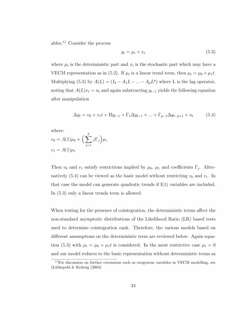
ables.11 Consider the process

yt = µt + xt (5.3)

where µt is the deterministic part and xt is the stochastic part which may have a

VECM representation as in (5.2). If µt is a linear trend term, then µt = µ0 +µ1t.

Multiplying (5.3) by A(L) = (Ik −A1L− ...−ApLp) where L is the lag operator,

noting that A(L)xt = ut and again substracting yt−1 yields the following equation

after manipulation

∆yt = v0 + v1t+ Πyt−1 + Γ1∆yt−1 + ...+ Γp−1∆yt−p+1 + ut (5.4)

where:

v0 = A(1)µ0 +( p∑j=1

jΓj

)µ1

v1 = A(1)µ1

Then v0 and v1 satisfy restrictions implied by µ0, µ1 and coefficients Γj. Alter-

natively (5.4) can be viewed as the basic model without restricting v0 and v1. In

that case the model can generate quadratic trends if I(1) variables are included.

In (5.3) only a linear trends term is allowed.

When testing for the presence of cointegration, the deterministic terms affect the

non-standard asymptotic distributions of the Likelihood Ratio (LR) based tests

used to determine cointegration rank. Therefore, the various models based on

different assumptions on the deterministic term are reviewed below. Again equa-

tion (5.3) with µt = µ0 + µ1t is considered. In the most restrictive case µt = 0

and our model reduces to the basic representation without deterministic terms as

11For discussion on further extensions such as exogenous variables in VECM modelling, see(Lutkepohl & Kratzig (2004)

34

in (5.2). The model could be applied in a situation without linear trends in the

levels of yt and if the variables in yt had equal means in levels. In a more realistic

setting µ1 = 0 is chosen. Following the reasoning in (5.4) above, we arrive at the

VECM form for yt

∆yt = Π(yt−1 − µ0) +

p−1∑j=1

Γj∆yt−j + ut

= v∗0 + Π(yt−1) +

p−1∑j=1

Γj∆yt−j + ut

= Π∗

yt−11

+

p−1∑j=1

Γj∆yt−j + ut

(5.5)

where Π∗ =[Π v∗0

]and v0∗ = −Πµ0. The intercept is included in the cointe-

grating vector (long-run relationship). This corresponds to the case where the

series have no trends in levels, but the means of the series are unequal. As above,

the intercept term can be absorbed into the cointegrating relation or left outside

(unrestricted). If however there is a linear deterministic trend in yt then µ1 6= 0.

If this trend is absent from the cointegrating relations but included in some in-

dividuals variable(s), then β′µ1 = 0 and thus Π(yt−1 − µ0 − µ1(t− 1)) reduces to

Π(yt−1 − µ0). The VECM form (5.2) now gives

∆yt = v0 + Πyt−1 +

p−1∑j=1

Γj∆yt−j + ut (5.6)

where v0 = −Πµ0 +( p∑j=1

jΓj

)µ1

Thus (5.6) assumes that the linear trend is orthogonal to the cointegration re-

lations. Finally, if an unrestricted linear trend term is allowed in equation (5.2)

35

the following VECM form is obtained

∆yt = v + Π∗

yt−1t− 1

+

p−1∑j=1

Γj∆yt−j + ut (5.7)

where Π∗ = α[β′ − β′µ1

]and v = −Πµ0 + (IK − Γ1 − ...− Γp−1)µ1

In (5.7) both the variables and the cointegrating relations are allowed to have lin-

ear trends. The reason a trend term may be required in the cointegrating relations

is that the growth rates of the variables in yt may differ. Finally, in addition to the

considered models, structural changes or breaks in the data generating process

have to be considered in model construction. Ignoring breaks in modelling may

lead to rejection of cointegration even if the variables are cointegrated. Therefore

including dummy variables for structural breaks in the deterministic part of the

VAR or VECM process may be justified especially in the case of a break at a

known point in time. This implies changes in the asymptotic distributions for

Johansen trace test for cointegration rank which have to be accounted for.

5.3 Testing for cointegration

As noted earlier, the rank of the matrix Π in the error correction model (5.2)

reveals the number of cointegrating vectors in the process yt. If rk(Π) = K,

all variables in the system are I(0) and the system is stationary. Similarly, if

rk(Π) = 0 then the term Πyt−1 disappears from (5.2) and the equation reduces to

an ordinary VAR in differences. In intermediate cases, i.e. when 0 < rk(Π) < K,

cointegration is present and a VECM presentation is suitable for cointegration

analysis.

36

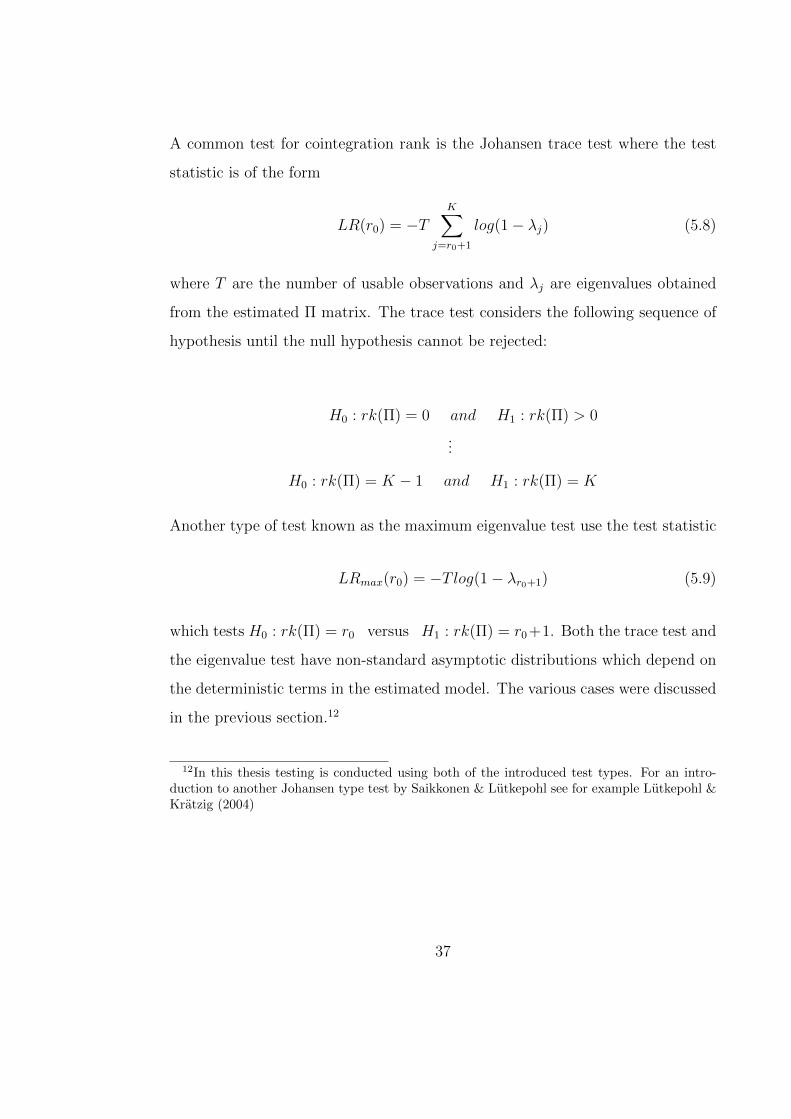
A common test for cointegration rank is the Johansen trace test where the test

statistic is of the form

LR(r0) = −TK∑

j=r0+1

log(1− λj) (5.8)

where T are the number of usable observations and λj are eigenvalues obtained

from the estimated Π matrix. The trace test considers the following sequence of

hypothesis until the null hypothesis cannot be rejected:

H0 : rk(Π) = 0 and H1 : rk(Π) > 0

...

H0 : rk(Π) = K − 1 and H1 : rk(Π) = K

Another type of test known as the maximum eigenvalue test use the test statistic

LRmax(r0) = −T log(1− λr0+1) (5.9)

which tests H0 : rk(Π) = r0 versus H1 : rk(Π) = r0+1. Both the trace test and

the eigenvalue test have non-standard asymptotic distributions which depend on

the deterministic terms in the estimated model. The various cases were discussed

in the previous section.12

12In this thesis testing is conducted using both of the introduced test types. For an intro-duction to another Johansen type test by Saikkonen & Lutkepohl see for example Lutkepohl &Kratzig (2004)

37

6 Data

This section introduces the data used in the empirical analysis. Sections three

and four presented motivation for the choice of house price determinants in em-

pirical modelling. Some additional arguments are presented below. The vector of

endogenous variables yt = (Pt Yt Lt IRt MIGt) consists of variables for dwelling

prices, household disposable income, household indebtedness, interest rates and

total net migration respectively. The data are quarterly observations reaching

from 1983/Q1 to 2012/Q4. The base year for all the index series is standard-

ised. The series for house prices, income and loan stock were transformed using

natural logarithms. The series were deflated by the cost-of-living index with the

exception of the total net migration.

6.1 House prices

The house price indices for the HMA are published by Statistics Finland.13 The

hedonic price indices separate the true price developments as opposed to price

developments originating from changes in dwelling characteristics over time. The

final index used in this thesis was constructed by linking three different indices

of old dwellings prices. The drawback is that the first of the series reaching from

1983 to 2001 considers flats where as the latter two include terraced housing as

well. Nevertheless, the constructed index should be a fairly good description of

the development of HMA housing prices in the sample period.

13Precise data sources concerning Statistics Finland data on house price and disposable in-come indices, the stock of house loans and total net migration presented in the references underStatistics Finland (b)-(f)

38

6.2 Income

Household (permanent) income is considered a major determinant of housing con-

sumption in most studies and is also included in this thesis. The quarterly series

for household disposable income is constructed by combining two index series

published by Statistics Finland. The first is the ’mean disposable monetary in-

come of a household-dwelling unit’ for each of the HMA municipalities separately.

The corresponding yearly figures for the HMA are computed by applying weights

according to the population size of each area and then summing over the four

municipalities. Since the regional-level data was unavailable for the entire period

of interest, national account data for disposable net income is used to extend the

series for the HMA disposable income between 1983 and 1995. The discontinuity

is obviously problematic, however presumably the development of inter-regional

income inequality between the HMA and the rest of the country was moderate

before the IT sector boom of the late 1990’s. Furthermore, the data for 2012 is

unavailable and the series was lengthened using again national level disposable

income data. Finally, the index of wage and salary earnings was used to estimate

the quarterly observations from the yearly income data.

6.3 Household indebtedness

Oikarinen (2007) argues that the stock of housing loans is an important source of

information concerning fundamentals that affect housing prices. First, increases

in perceived permanent income induce households to smooth consumption over

lifetime which leads to increased borrowing. Similarly, income uncertainty re-

flects into borrowing behaviour because of precautionary saving. In addition,

current and expected interest rate levels should reflect on household borrowing.

Finally, borrowing should reflect changes in the household liquidity constraints as

39

improved availability of credit should relax these constraints. For these reasons

it is justified to add a variable describing household indebtedness and the degree

of liquidity constraints faced by households.

0

20

40

60

80

100

120

140

160

1983 1986 1989 1992 1995 1998 2001 2004 2007 2010

2005

=100

Disposable income

Dwelling prices

Household debt-to-equity

Figure 5: Dwelling prices, disposable income & household debt-to-equity

A variable describing the household debt-to-equity ratio is constructed using data

on quarterly stock of household mortgage loans provided by Statistics Finland.

The data is only available at national level, thus it has to be assumed that HMA

borrowing behaviour resembles national level development.14 The stock of mort-

gage loans is in proportion to the household disposable net income in order to

scale the proportion of credit in housing transactions.

14Support for this assumption is provided in Oikarinen (2007, 106)

40

6.4 Interest rates

The interest rate series provided by the Bank of Finland describe the average

interest rates on mortgages to households and non-profit organisations. The

after-tax nominal mortgage rate is computed as i(1− T ) where i is the nominal

mortgage rate and T is the tax rate. The capital tax rate is used as T from

1993 onwards. Before the year 1993 an average marginal income tax rate was

computed to represent T . The average marginal income tax rate was constructed

by dividing collected taxes from labour income and social security payments by

employee compensation from the annual national accounts by Statistics Finland.

6.5 Demography

Englund (2011, 45) notes that the stock of housing has two main dimensions: the

number of dwellings and the quality and size of the average dwelling. An increase

in income would primarily affect the demand for quality, whereas a growing pop-

ulation would demand more units. Then, income and demography should have a

separate influence on dwelling prices. In this thesis, the total net migration in the

Helsinki region is chosen as the ’demographic’ variable. Supposedly, migration

has caused pressure on house prices in the metropolitan area, especially due to

increased immigration to Finland in the recent years. Moreover, total net mi-

gration should reflect the ’pull’ of the metropolitan area labour markets and the

effect of this workforce on HMA dwelling prices especially in the 1990’s. Instead

of the HMA, the Helsinki region is selected as it is considered an employment area

rather than HMA alone. The quarterly total net migration figures were provided

by Statistics Finland.15

15The total net migration series used in the econometric model was seasonally adjusted usingDemetra+

41

The series for real dwelling prices (Pt), household disposable income (Yt) and

the household debt-to-equity (Lt) are presented in figure 5. The average real

mortgage rates (IRt) and the non-adjusted total net migration series (MIGt) are

pictured in figure 6.

-4

-2

0

2

4

6

8

-1000

0

1000

2000

3000

4000

5000

6000

1983 1986 1989 1992 1995 1998 2001 2004 2007 2010

Rea

l mo

rtga

ge r

ate,

%

Tota

l net

mig

rati

on

Total net migration Real mortgage rate

Figure 6: Real mortgage rate & total net migration

All the above variables used in the empirical analysis are demand side variables.

As noted in previous sections, the supply side is often hard to account for. At-

tempts to model house prices with a construction cost index were made, but the

variable was eventually left out since it added no information to the cointegrated

system. On the contrary, inclusion of construction costs produced nonsensical

results for the econometric model. According to test results, the two variable

system of real dwelling prices and real construction costs is not cointegrated.

The result is not surprising since real construction costs have been fairly stable

throughout the sample period.

42

7 Econometric Analysis

This section presents the results from the cointegration analysis.16 The analysis

is conducted using the methodology introduced in section five on the time series

vector described in the previous section

yt = [Pt Yt Lt IRt MIGt]′

The stationarity of the variables in vector yt was first studied both via visual

inspection and the augmented Dickey-Fuller (ADF) unit root test. None of the

time series seem stationary (see figures 5 & 6). The original series for total net

migration exhibits notable seasonal variation and was seasonally adjusted prior

to estimation. Due to the shape of the time series, a constant and a trend were

added to the test regressions for Pt, Yt and Lt. Similarly, the IRt and MIGt series

were modelled with a constant. Selected unit root test results are summarised

in Table 1. Optimal lag length was chosen according to AIC, BIC and Hannan-

Quinn criteria. The results of the tests indicate that unit roots cannot be rejected

in the levels of any of the variables. With the differenced series, Pt, Yt and Lt

were now estimated with a constant and IRt and MIGt without deterministic

terms. The differenced series tested stationary with the exception of the Lt series.

With variation of the lag length around the initial value of ρ = 3, the tests clearly

rejected unit root. Thus, modelling could continue by treating all the variables

as I(1) variables. Given these integration and trending properties, cointegration

between the variables is possible.

16JMulTi & gretl software were used for estimation

43

Table 1: Augmented Dickey-Fuller tests

Variable Deterministic Lags Test CVterms 1% 5% 10%

P constant + trend 1 -2.2357 -3.96 -3.41 -3.13∆ P constant 0 -4.6504 -3.43 -2.86 -2.57

Y constant + trend 4 -2.6096 -3.96 -3.41 -3.13∆Y constant 3 -3.4349 -3.43 -2.86 -2.57

L constant + trend 4 -1.4486 -3.96 -3.41 -3.13∆L constant 3 -2.4923 -3.43 -2.86 -2.57∆L constant 2 -4.6106 -3.43 -2.86 -2.57

IR constant 1 -2.3091 -3.43 -2.86 -2.57∆ IR none 0 -8.3301 -2.56 -1.94 -1.62

MIG constant 1 -2.0359 -3.43 -2.86 -2.57∆ MIG none 0 -14.7612 -2.56 -1.94 -1.62

Asymptotic critical values from Davidson & MacKinnon (1993)

A VAR model with a lag length of two, a constant but no trend and with centered

seasonal dummy variables was estimated for yt. Lag length was again chosen by

appropriate information criteria. The specification was used to test for cointegra-

tion employing both the Johansen trace test and the maximum eigenvalue test.

The Likelihood Ratio (LR) based tests for cointegration rank are based on a

VAR model where all short-run dynamics, dummy variables and other determin-

istic components have been concentrated out (Juselius 2006, 131). Further, the

distribution of the test statistic is non-standard and based on simulations. Thus,

including a deterministic term (unrestricted constant) in the VAR process implies

changes in the asymptotic distributions for Johansen trace test for cointegration

rank. The critical values and p-values for the trace test are obtained by comput-

ing the respective response surface according to Doornkik (1998). The results are

summarised in Table 2. Both test statistics indicate a cointegrating rank of one

44

Table 2: Cointegration test results for VAR(2)

Trace test L-max test

H0 Test statistic p-value Test statistic p-value

r = 0 89, 927 [0, 0004] 44, 624 [0, 0009]r = 1 45, 302 [0, 0840] 25, 798 [0, 0817]r = 2 19, 504 [0, 4680] 11, 282 [0, 6290]r = 3 8, 2226 [0, 4492] 7, 3811 [0, 4539]r = 4 0, 84156 [0, 3590] 0, 84156 [0, 3590]

implying that there is one stationary linear vector between the variables.17 Next,

a VECM(1) based on the VAR(2), that is, with one lag in differences under a rank

restriction r = 1 was estimated. The estimated cointegrating vector normalised

with respect to Pt is shown in Table 3. The estimated β vector can be written as

a long-run relation of the form

Pt = 0, 468 Yt + 0, 430 Lt − 0, 027 IRt + 0, 00006 MIGt (7.1)

The long-run real house price equilibrium equation presents expected results.

First, all the coefficients on the cointegrating vector are significant. The coeffi-

cients have the expected sign and magnitude, meaning that they are in line with

findings from previous studies. According to (7.1), a one per cent increase in real

disposable income Yt increases prices by 0.47 %, holding all else constant. This

result is almost identical to Oikarinen (2007). This is no surprise since the data

and time period in the study are very similar to this thesis. For example, Kuis-

manen et al. (1999) and Kosonen (1997) found notably higher long-run income

17Detailed results in Appendix A1

45

elasticity of housing price level of around 0.81 and 1.4, respectively. The elastic-

ity of house prices with respect to household debt-to-equity (Lt) is 0.43 implying

that the impact of loosening liquidity constraints is equally important as house-

hold income in explaining dwelling prices. Furthermore, house price increases

obviously require higher mortgage loans, thus the close connection between the

variables comes as no surprise.

Table 3: The cointegrating vector (β) and loading parameters (α) for VECM(1)

Pt Yt Lt IRt MIGt

β 1 -0,468 -0,430 0,027 -0,00006(-2,4) (-5,9) (2,9) (2,0)

α -0,094 -0,054 0,063 -0,477 48,019(-5,2) (-3,0) (3,4) (-1,2) (0,17)

*t-values in parentheses; full model summary in Appendix A2

According to the relation a percentage-point increase in the real mortgage rate

reduces prices by 2.7 %. The moderate effect of real mortgage rates - a key

component of user cost - is somewhat surprising. On the other hand, more re-

cent evidence on Finnish data (Hofmann (2004), Oikarinen (2007) and Adams &

Fuss (2010)) find equivalently weak impact for real interest rates. It is possible

that the debt-to-equity ratio captures some of the effect. Moreover, Oikarinen

(2007, 136) evaluates that especially if the effect of expected future interest rates

on house prices is notable, then the anticipated effect of current interest rate is

relatively small. Finally, the coefficient on MIGt implies that an increase of one

person in total net migration to the Helsinki region results in a 0.003 % increase

in HMA housing prices, ceteris paribus. Equivalently an increase of 1000 in total

net migration on a given quarter would raise housing prices by 3 %. Considering

46

the migration flow of the previous decades, it would therefore seem that HMA

house prices have been significantly affected by migration. For comparison, a

model excluding total net migration was also estimated. The results were very

similar to the ones presented with the exception that, expectedly, the coefficient

for disposable income now captured some of the effect previously included in the

migration variable. This suggests that multicollinearity between these variables

might be significant and the estimates of the price relation have to be considered

with caution.

The loading parameters α reported in Table 3 provide some support to the long-

run model. The result for Pt suggests that dwelling prices adjust 9.4% per quarter

towards the long-run relationship following a shock to the system. This equals to

annual adjustment of approximately 33%. The estimate of sluggish house prices

adjustment is well in line with other housing market studies. Similarly the debt-

to-equity ratio (Lt) converges slowly towards long-run equilibrium, at a rate of

6.3% per quarter. This amounts to 23% annually. The remaining loading pa-

rameters are either insignificant or of the wrong sign. Finally, an error-correction

model for real house price movements presented in Appendix A3 shows that

roughly 60% of the variation in quarterly house prices can be explained by the

lagged explanatory variables.

Multiple diagnostic tests were conducted on the specification (see Appendix A4).

Visual inspection of the individual residual series, autocorrelation and partial au-

tocorrelation functions gives no reason for major concern. The single equation

Ljung-Box tests indicate some signs of residual autocorrelation for the disposable

income series. The autocorrelation functions do not cross the ±2√T approxi-

mate 95 % confidence bounds at lower lags for the other series and therefore do

47

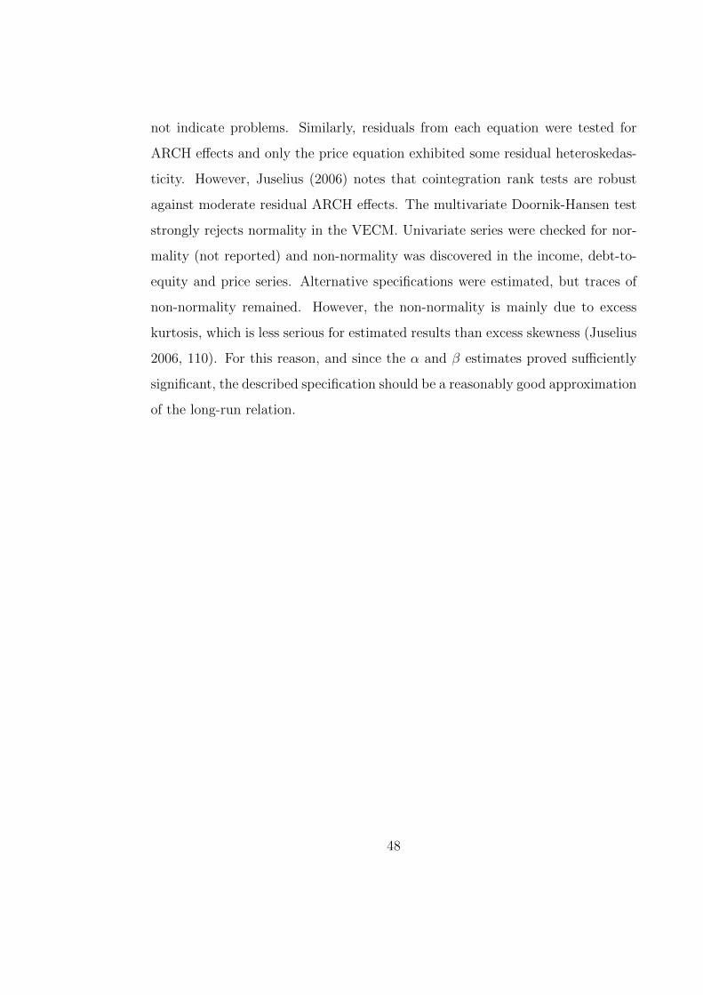
not indicate problems. Similarly, residuals from each equation were tested for

ARCH effects and only the price equation exhibited some residual heteroskedas-

ticity. However, Juselius (2006) notes that cointegration rank tests are robust

against moderate residual ARCH effects. The multivariate Doornik-Hansen test

strongly rejects normality in the VECM. Univariate series were checked for nor-

mality (not reported) and non-normality was discovered in the income, debt-to-

equity and price series. Alternative specifications were estimated, but traces of

non-normality remained. However, the non-normality is mainly due to excess

kurtosis, which is less serious for estimated results than excess skewness (Juselius

2006, 110). For this reason, and since the α and β estimates proved sufficiently

significant, the described specification should be a reasonably good approximation

of the long-run relation.

48

8 Conclusions

Real house prices in the HMA have risen by approximately 99 percent between

1983 and the end of 2012. The rapid increases in house prices especially after the

early 1990’s depression has regularly brought forward the topic of overheating

in the housing market. Even though the speed of real house price appreciation

has not been as fast as during the bubble of the late 1980’s, it is understandable

that the unprecedented price bubble is still remembered in discussion. In Fin-

land, discussion concerning house prices is especially centred around the Helsinki

metropolitan area where the highest price rises have often been witnessed. Dur-

ing the recent years, real dwelling prices in the HMA have actually bypassed the

peak levels recorded in 1989. The question then remains, whether the price level

in the HMA is sustainable in the long-run.

The cointegration analysis of section seven presented a long-run equilibrium real

house price level towards which real house prices should adjust. To answer the

question on possible overvaluation in the HMA housing markets, figure 7 plots

the actual real house prices and the fit from the estimated long-run relation from

section seven for the period under consideration. Clearly, the actual prices have

far exceeded the long-run price level determined by fundamental factors of house

prices applied in this thesis for most of the sample period. At the peak of 1989,

the actual price level in the HMA was around 80% above the estimated equi-

librium level. Conversely, actual prices were well in line with the fundamentals

between 1992 and 1996, the time period which roughly coincides with economic

downturn in Finland. Since 1997, actual prices have exceeded the long-run fun-

damental level by approximately 45% on average. By the end of 2012, real house

prices were 32% above the estimated long-run level. Based on these numbers, it

seems that real dwelling prices in the HMA have been significantly overvalued

49

for a prolonged period. Actual prices have been significantly above the level sug-

gested by fundamental determinants thus fulfilling the definition of a price bubble.

0

20

40

60

80

100

120

140

1983 1986 1989 1992 1995 1998 2001 2004 2007 2010

Real house prices

Estimated long-run equilibrium

Figure 7: HMA real house prices & the estimated long-run equilibrium prices

It should be emphasized that a high price level on its own does not imply over-

valuation. As shown in figure 7, more recently the long-run equilibrium level has

risen at approximately the same rate as the actual price level, despite having

been nearly constant between 1983 and 2004. This rise of the last decade or

so in the long-run level is attributable to notable decreases in real interest rates

and equivalently rapid expansion in household indebtedness signalling loosening

household liquidity constraints. As shown by the econometric analysis, household

real disposable income seems to be an important determinant of house prices, but

it has been fairly constant or even declining in the previous years. Therefore it

has not been the major ’push’ behind real house price rises. On the other hand,

increasing total net migration to the HMA has caused notable growth in the long-

run price level.

50

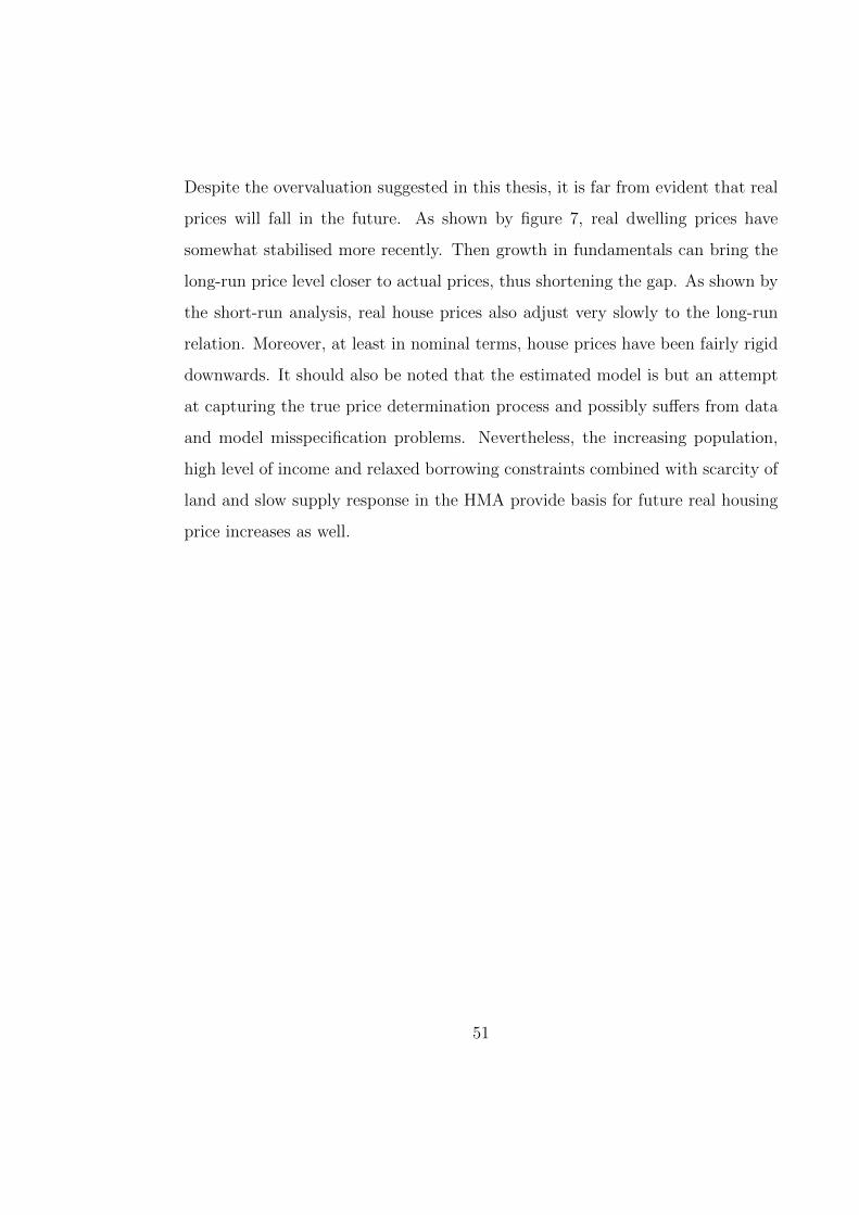
Despite the overvaluation suggested in this thesis, it is far from evident that real

prices will fall in the future. As shown by figure 7, real dwelling prices have

somewhat stabilised more recently. Then growth in fundamentals can bring the

long-run price level closer to actual prices, thus shortening the gap. As shown by

the short-run analysis, real house prices also adjust very slowly to the long-run

relation. Moreover, at least in nominal terms, house prices have been fairly rigid

downwards. It should also be noted that the estimated model is but an attempt

at capturing the true price determination process and possibly suffers from data

and model misspecification problems. Nevertheless, the increasing population,

high level of income and relaxed borrowing constraints combined with scarcity of

land and slow supply response in the HMA provide basis for future real housing

price increases as well.

51

References

[1] Abraham, J. M. & Hendershott, P. H. 1996. Bubbles in Metropolitan Housing

Markets. Journal of Housing Research 7 (2), 191-207.

[2] Adams, Z. & Fuss, R. 2010. Macroeconomic determinants of international

housing markets. Journal of Housing Economics 19 (1), 38-50.

[3] Benjamin, John D., Chinloy, Peter & Jud, G. Donald 2004. Why Do House-

holds Concentrate Their Wealth in Housing? Journal of Real Estate Re-

search 26 (4), 329-343.

[4] Bessone, A.-J., Boissinot J. & Heitz, B. 2005. Marche immobilier: voit-on

une bulle? Note de Conjoncture, INSEE.

[5] Borowiecki, Karol J. 2009. The Determinants of House Prices and Con-

struction: An Empirical Investigation of the Swiss Housing Economy Inter-

national Real Estate Review 12 (3), 193-220.

[6] Barot, Bharat & Takala, Kari. 1998. House Prices and Inflation: A Cointe-

gration Analysis for Finland and Sweden Bank of Finland Discussion Papers

12/98.

[7] Capozza, D. R., Hendershott, P. H., Mack, C. & Mayer, C. J. 2002. Deter-

minants of Real House Price Dynamics NBER Working Paper, 9262.

[8] Case, Karl E., Quigley, John M. & Shiller, Robert J. 2001. Comparing wealth

effects: the stock market versus the housing market. National Bureau of Eco-

nomic Research. Working Paper No. 8606.

[9] Case, Karl E. & Shiller, Robert J. 2003. Is There a Bubble in the Housing

Market? Brookings Papers on Economic Activity 2, 299-362.

52

[10] Davidson, R. & MacKinnon, J. 1993. Estimation and Inference in Econo-

metrics. Oxford University Press, London.

[11] DiPasquale, Denise & Wheaton, William C. 1994. Housing Market Dynamics

and the Future of Housing Prices. Journal of Urban Economics 35, 1-27.

[12] Doornik, J.A. 1998. Approximations to the asymptotic distributions of coin-

tegration tests. Journal of Economic Surveys 12, 573-593.

[13] Engle, Robert E. & Granger Clive W. J. 1987. Cointegration and Error

Correction: Representation, Estimation, and Testing. Econometrica, vol. 55,

No. 2, 251-276.

[14] Englund, Peter 2011. Swedish house prices in an international perspective. In

The Riksbank’s inquiry into the risks in the Swedish housing market. Sveriges

Riksbank, 23-66.

[15] Ganoulis, Ioannis & Giuliodori, Massimo 2010. Financial liberalization and

house price dynamics in Europe. Applied Economics, 1-18, (iFirst) Rout-

ledge.

[16] Girouard, Nathalie, Kennedy, Mike, van den Noord, Paul & Andre,

Christophe 2006. Recent House Price Developments: The Role of Funda-

mentals. OECD, Economic Department Working Paper No. 475

[17] Goodhart, Charles & Hofmann, Boris 2007. House Prices and the Macroe-

conomy: Implications for Banking and Price Stability. Oxford University

Press: Oxford.

[18] Hendry, D.F. 1984. Econometric modelling of house prices in the United

Kingdom. In Hendry, D.F. & Wallis, K.F. (Ed.), Econometrics and Quanti-

tative Economics. Oxford: Basil Blackwell, 211-252.

53

[19] Hilbers, Paul, Hoffmaister, Alexander W., Banerji, Angana & Shi, Haiyan

2008. House price developments in Europe: A comparison. IMF working

paper, WP/08/211.

[20] Himmelberg, Charles, Mayer Christopher & Sinai, Todd 2005. Assessing

High House Prices: Bubbles, Fundamentals and Misperceptions. The Journal

of Economic Perspectives, Vol. 19, No. 4, 67-92.

[21] Hofmann, Boris 2004. The Determinants of Bank Credit in Industrialized

Countries: Do Property Prices Matter?. International Finance, 7(2), 203-

234.

[22] Holly, Sean & Jones, Natasha 1997. House prices since the 1940s: cointegra-

tion, demography and asymmetries. Economic Modelling 14 (4), 549-565.

[23] Hort, Katinka 1998. The Determinants of Urban House Price Fluctuations

in Sweden 1968-1994. Journal of Housing Economics 7, 93-120.

[24] Juselius, Katarina 2006. The Cointegrated VAR model: Methodology and

Applications. Oxford Univeristy Press.

[25] Kosonen, Katri 1997. House Price Dynamics in Finland. Labour Institute

for Economic Research, Discussion Papers 137: Helsinki.

[26] Kuismanen, Mika, Laakso, Seppo & Loikkanen, Heikki A. 1999. Demographic

Factors and the Demand for Housing in the Helsinki Metropolitan Area. Gov-

ernment Institute for Economic Research, Working Papers No. 191.

[27] Laakso, Seppo 2000. Regional Housing Market in Boom and Bust: the Ex-

perience of Finland. Pellervo Economic Research Institute Reports No. 169.

[28] Laakso, Seppo & Loikkanen, Heikki A. 2004. Kaupunkitalous. Gaudeamus,

Helsinki.

54

[29] Laakso, Seppo 2007. Tonttitarjonta ja asuntomarkkinat

paakaupunkiseudulla. Helsingin kaupungin talous- ja suunnittelukeskuksen

julkaisuja 3/2007.

[30] Lutkepohl, Helmut & Kratzig, Markus 2004. Applied Time Series Econo-

metrics, Cambridge University Press.

[31] Mankiw, Gregory N. & Weil, David N. 1989. The baby boom, the baby bust,

and the housing market. Regional and Urban Economics 19 (2), 235-258.

[32] McQuinn, K. 2004. A model of the Irish housing sector. Central Bank of

Ireland Technical paper, 1/RT/04 .

[33] Meese, Richard & Wallace, Nancy 2003. House Price Dynamics and Market

Fundamentals: The Parisian Housing Market. Urban Studies 40 (5-6), 1027-

1045.

[34] Niemi, Erkki & Sandstrom, Taru 2007. Suomen kansallisvarallisuuden

rakenne on muuttunut. Tieto & Trendit 12/2007. Tilastokeskus.

[35] Nivalainen, Satu & Vuori, Pekka 2012. Metropolialueen vaesto ja muut-

toliike. In Loikkanen, Heikki A., Laakso Seppo & Susiluoto Ilkka (Ed.),

Metropolialueen talous - Nakokulmia kaupunkitalouden ajankohtaisiin ai-

heisiin. Helsingin kaupunki. Tietokeskus, 157-183.

[36] Oikarinen, Elias 2007. Studies on housing price dynamics. Doctoral Thesis.

Turku School of Economics. Series A-9:2007.

[37] Pere, Pekka & Takala, Kari 1991. Testing the cointegration of house and

stock prices in Finland. Finnish Economic Papers, 4 (1), 33-51.

55

[38] Poterba, James M. 1984. Tax Subsidies to Owner-Occupied Housing: An

Asset-Market Approach. The Quarterly Journal of Economics 99 (4), 729-

752.

[39] Poterba, James M. 1991. House Price Dynamics: The Role of Tax Policy

and Demography. Brookings Papers on Economic Activity 2, 143-203.

[40] Statistics Finland (a), PX-Web databases: Household-dwelling units by num-

ber of persons and type of building 1985-2012.

http://pxweb2.stat.fi/database/StatFin/asu/asas/asas_en.asp

[41] Statistics Finland (b), PX-Web databases: Prices of dwellings in housing

companies.

http://193.166.171.75/Database/StatFin/Asu/ashi/ashi_fi.asp

[42] Statistics Finland (c), PX-Web databases: Mean disposable monetary income

of a household-dwelling unit 1995-2011.

http://pxweb2.stat.fi/database/StatFin/tul/tjkt/tjkt_en.asp

[43] Statistics Finland (d), PX-Web databases: Gross domestic product and -

national income at current prices 1975-2012.

http://pxweb2.stat.fi/database/StatFin/kan/vtp/vtp_en.asp

[44] Statistics Finland (e), PX-Web databases: Credits by purpose of use and

sector of lender and borrower by quarter.

http://pxweb2.stat.fi/database/StatFin/rah/lkan/lkan_en.asp

[45] Statistics Finland (f), PX-Web databases: General government’s total rev-

enue and -expenditure 1975-2012.

http://pxweb2.stat.fi/database/StatFin/kan/vtp/vtp_en.asp

56

[46] Wilhelmsson, M. 2008. Regional house prices: An application of a two-

equation model to the Swedish housing market. International Journal of Hous-

ing Markets and Analysis, 1 (1), 33-51.

57

9 Appendix

A1: Cointegration tests

Johansen test:

Number of equations = 5

Lag order = 2

Estimation period: 1983:3 - 2012:4 (T = 118)

Case 3: Unrestricted constant

Log-likelihood = 358,8 (including constant term: 23,9303)

Rank Eigenvalue Trace test p-value L-max test p-value

0 0, 31489 89, 927 [0, 0004] 44, 624 [0, 0009]

1 0, 19638 45, 302 [0, 0840] 25, 798 [0, 0817]

2 0, 091179 19, 504 [0, 4680] 11, 282 [0, 6290]

3 0, 060635 8, 2226 [0, 4492] 7, 3811 [0, 4539]

4 0, 0071065 0, 84156 [0, 3590] 0, 84156 [0, 3590]

Corrected for sample size (df = 104)

Rank Trace test p-value

0 89, 927 [0, 0007]

1 45, 302 [0, 1013]

2 19, 504 [0, 4845]

3 8, 2226 [0, 4580]

4 0, 84156 [0, 3651]

eigenvalue 0,31489 0,19638 0,091179 0,060635 0,0071065

A2: Summary of estimated VECM system

VECM system, lag order 2

Maximum likelihood estimates, observations 1983:3–2012:4 (T = 118)

Cointegration rank = 1

Case 3: Unrestricted constant

Cointegrating vectors (standard errors in parentheses)

PPPt−1 1,00000

(0,000000)

YYYt−1 −0,468241

(0,192910)

LLLt−1 −0,430294

(0,0728385)

IRt−1 0,0272662

(0,00937487)

MIGMIGMIGt−1 −6,10978e–005

(3,02370e–005)

Adjustment vectors

PPPt−1 1,00000

YYYt−1 0,575431

LLLt−1 −0,669913

IRt−1 5,09357

MIGMIGMIGt−1 −512,730

Log-likelihood = 1,27916

Determinant of covariance matrix = 6,73306e–007

AIC = 1, 1648

BIC = 2, 8084

HQC = 1, 8321

A3: ECM for Pt

Equation 1: ∆P

Coefficient Std. Error t-ratio p-value

const 0,0222188 0,00479780 4,6310 0,0000

∆Pt−1 0,663906 0,0741064 8,9588 0,0000

∆Yt−1 0,489090 0,194858 2,5100 0,0136

∆Lt−1 0,893878 0,187691 4,7625 0,0000

∆IRt−1 −0,00844838 0,00427764 −1,9750 0,0508

∆MIGt−1 −8,14252e–007 5,79394e–006 −0,1405 0,8885

S1 0,0245732 0,00649477 3,7835 0,0003

S2 0,0168664 0,00726083 2,3229 0,0221

S3 0,0197093 0,00671300 2,9360 0,0041

EC1 −0,0936540 0,0178754 −5,2393 0,0000

Mean dependent var 0,005752 S.D. dependent var 0,037218

Sum squared resid 0,059421 S.E. of regression 0,023456

R2 0,633355 Adjusted R2 0,602802

ρ −0,044641 Durbin–Watson 2,082316

A4: Diagnostic tests

Equation 1 (Pt): Ljung-Box Q’ = 1,17792 with p-value = 0,882

Equation 2 (Yt): Ljung-Box Q’ = 12,4779 with p-value = 0,0141

Equation 3 (Lt): Ljung-Box Q’ = 9,36776 with p-value = 0,0525

Equation 4 (IRt): Ljung-Box Q’ = 5,58595 with p-value = 0,232

Equation 5 (MIGt): Ljung-Box Q’ = 1,91022 with p-value = 0,752

Test for ARCH of order 4

Equation 1 (P):

coefficient std. error t-ratio p-value

alpha(0) 0,000372682 0,000111820 3,333 0,0012 ***

alpha(1) 0,199974 0,0948074 2,109 0,0372 **

alpha(2) 0,188053 0,0966682 1,945 0,0543 *

alpha(3) 0,0238752 0,0966305 0,2471 0,8053

alpha(4) -0,139651 0,0948140 -1,473 0,1437

Null hypothesis: no ARCH effect is present Test statistic: LM = 11,4346 with

p-value = 0,0220905

Test for ARCH of order 4

Equation 2 (Y):

coefficient std. error t-ratio p-value

alpha(0) 0,000432972 0,000177692 2,437 0,0164 **

alpha(1) 0,0230314 0,0950306 0,2424 0,8090

alpha(2) -0,0410366 0,0949563 -0,4322 0,6665

alpha(3) 0,0488027 0,0949450 0,5140 0,6083

alpha(4) 0,127884 0,0950550 1,345 0,1813

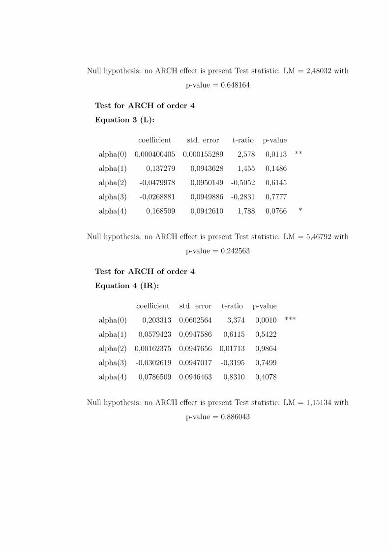
Null hypothesis: no ARCH effect is present Test statistic: LM = 2,48032 with

p-value = 0,648164

Test for ARCH of order 4

Equation 3 (L):

coefficient std. error t-ratio p-value

alpha(0) 0,000400405 0,000155289 2,578 0,0113 **

alpha(1) 0,137279 0,0943628 1,455 0,1486

alpha(2) -0,0479978 0,0950149 -0,5052 0,6145

alpha(3) -0,0268881 0,0949886 -0,2831 0,7777

alpha(4) 0,168509 0,0942610 1,788 0,0766 *

Null hypothesis: no ARCH effect is present Test statistic: LM = 5,46792 with

p-value = 0,242563

Test for ARCH of order 4

Equation 4 (IR):

coefficient std. error t-ratio p-value

alpha(0) 0,203313 0,0602564 3,374 0,0010 ***

alpha(1) 0,0579423 0,0947586 0,6115 0,5422

alpha(2) 0,00162375 0,0947656 0,01713 0,9864

alpha(3) -0,0302619 0,0947017 -0,3195 0,7499

alpha(4) 0,0786509 0,0946463 0,8310 0,4078

Null hypothesis: no ARCH effect is present Test statistic: LM = 1,15134 with

p-value = 0,886043

Test for ARCH of order 4

Equation 5 (MIG):

coefficient std. error t-ratio p-value

alpha(0) 120208 34010,9 3,534 0,0006 ***

alpha(1) 0,233980 0,0956925 2,445 0,0161 **

alpha(2) -0,0559097 0,0979680 -0,5707 0,5694

alpha(3) -0,0878121 0,0979412 -0,8966 0,3719

alpha(4) -0,0226585 0,0956874 -0,2368 0,8133

Null hypothesis: no ARCH effect is present Test statistic: LM = 7,45238 with

p-value = 0,113827

Test for normality of residual

Residual correlation matrix, C (5 x 5)

1,0000 0,083020 0,099304 0,12541 -0,093908

0,083020 1,0000 -0,86979 0,19012 -0,16650

0,099304 -0,86979 1,0000 0,0045213 0,098181

0,12541 0,19012 0,0045213 1,0000 -0,035448

-0,093908 -0,16650 0,098181 -0,035448 1,0000

Eigenvalues of C

0,0942675 0,834918 0,962147 1,17908 1,92959

Doornik-Hansen test

Chi-square(10) = 113,633 [0,0000]

4.3

4.4

4.5

4.6

Diagram of fit and residuals for Y

0 20 40 60 80 100 120

−0.

10−

0.05

0.00

0.05

0 2 4 6 8 10 12

−0.

20.

40.

8

Lag

ACF Residuals

2 4 6 8 10 12

−0.

10.

1

Lag

PACF Residuals

3.8

4.0

4.2

4.4

4.6

4.8

Diagram of fit and residuals for P

0 20 40 60 80 100 120

−0.

050.

000.

05

0 2 4 6 8 10 12

−0.

20.

40.

8

Lag

ACF Residuals

2 4 6 8 10 12

−0.

10.

1

Lag

PACF Residuals

4.2

4.4

4.6

4.8

5.0

Diagram of fit and residuals for L

0 20 40 60 80 100 120

−0.

050.

000.

050.

10

0 2 4 6 8 10 12

−0.

20.

40.

8

Lag

ACF Residuals

2 4 6 8 10 12

−0.

10.

1

Lag

PACF Residuals

−2

02

46

Diagram of fit and residuals for IR

0 20 40 60 80 100 120

−1.

00.

00.

51.

01.

5

0 2 4 6 8 10 12

−0.

20.

41.

0

Lag

ACF Residuals

2 4 6 8 10 12

−0.

20.

0

Lag

PACF Residuals

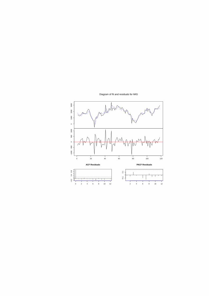
010

0020

0030

00

Diagram of fit and residuals for MIG

0 20 40 60 80 100 120

−10

00−

500

050

010

00

0 2 4 6 8 10 12

−0.

20.

40.

8

Lag

ACF Residuals

2 4 6 8 10 12

−0.

10.

1

Lag

PACF Residuals