ANOTHER INCONVENIENT TRUTH:

Climate change and migration in sub-Saharan Africa∗

Luca Marchiori † Jean-François Maystadt‡ Ingmar Schumacher§

June 21, 2010

Abstract

This paper analyzes the effects of climate change on international migration. Theoretically, we

show how climate change induces rural-urban migration that subsequently triggers international

migration. Empirically, based on annual, cross-country panel data for sub-Saharan Africa, our re-

sults suggest that climate change increased internal and international migration. Moreover, when

endogeneity is dealt with, urbanization mitigates the effect of climate change oninternational mi-

gration. Temperature and rainfall variations caused a total displacement of 2.35 million people in

net terms over the period 1960-2000 in sub-Saharan Africa, and predicted climate variations would

lead to anadditional annualdisplacement of 1.4 million people.

Keywords: International migration, urbanization, rural-urban migration, climate change, sub-Saharan Africa.

JEL Classification: F22, Q54, R13.

∗For helpful suggestions and comments we would kindly like tothank Luisito Bertinelli, Frédéric Docquier, Gilles Du-ranton, Giordano Mion, Dominique Peeters, Eric Strobl, Jacques Thisse as well as the participants at the Annual Conferenceof the European Society for Population Economics (June 2010).

†CREA, University of Luxembourg, and IRES, Université catholique de Louvain.E-mail: luca.marchiori@uni.lu.‡International Food Policy Research Institute (IFPRI), Washington DC.E-mail: J.F.Maystadt@cgiar.org.§Central Bank of Luxembourg, 2 Boulevard Royal, L-2983 Luxembourg.E-mail: ingmar.schumacher@bcl.lu.

1 Introduction

The analysis of the impacts of climate change has brought to light many inconvenient truths, ranging from a

reduction in biodiversity over melting ice caps to an increasing amount of extreme events. However, out of these

many inconvenient truths, none has yet seen as much media coverage as the impact of climate change on human

migration. To lose ones homeland to the forces of nature which mankind battled so eagerly against during the last

centuries seems to induce a sense of helplessness and dependency thatwas almost to be forgotten. Indeed, the

amount of people that have to leave their homes due to changes in local climatesis reported to be everything else

but negligible. Early works by El-Hinnawi (1985, 4) have first advanced the figure of 15 million people annually

that had to move as a result of floods during the 70s. Following the revision to10 million given by Jacobson

(1988), Myers (1996) increased the number of environmental refugees to 25 million for the sole year of 1995, of

which 18 million would originate from Africa. These authors also predict increasing risk in the future. A sea level

rise of one meter would produce between 50 million (Jacobson, 1988) to 200million environmental refugees

(Myers, 1996).1 In addition to flooding, climate change induces much broader phenomena, including the change

in the levels and the variability of precipitations and average temperature as well as the increased occurrence of

extreme weather events (Boko et al., 2007). Despite the very comprehensive overview of the Intergovernmental

Panel on Climate Change (IPCC) fourth report, the lack of robust evidence regarding the relationship between

migration and climate change is unfortunate (Boko et al., 2007, 450). In its 2010 World Development Report on

Development and Climate Change, the World Bank (2010 : 108-109) underlines that these “estimates are based

on broad assessments of people exposed to increasing risks rather thananalyses of whether exposure will lead

them to migrate.” The general knowledge of the effect of climate change onmigration is indeed surprisingly

limited, especially for a topic which is so very much at the heart of the modern, international debate. The only

studies that investigate environmental motives for migration in Africa are Barrios et al. (2006) and those that

analyze other motives are Hatton and Williamson (2003). It is, therefore, the objective of this article to provide

a theoretical and empirical analysis of the impact of climate change on migration.Based upon the empirical

analysis we also forward a tentative estimate of the number of environmental refugees in Africa between 1965

and 2000, as well as predictions until 2099.

What are the stylized facts that a study of rural-urban and urban-international migration should integrate?

Firstly, it is well-known that gradual climate change bears the strongest direct impacts on the agricultural activi-

ties, whereas the manufacturing sector is less hurt (IPCC, 2007). Thus, countries with a large dependency on the

agricultural sector are particularly vulnerable to climate change (Deschenes and Greenstone, 2007; World Bank,

2010). We should expect migration from the rural to the urban areas, together with mobility from the agricultural

to the non-agricultural sector. Climate change is, therefore, likely to fosterurbanization (Barrios et al 2006). As

1The term “environmental refugee” is itself a debate. The distinction between refugee and migrant is an importantpolicy debate, notably in terms of assistance and protection, see Black (2001), McGregor (1993), Kibreab (1997) or Suhrke(1994). In the rest of the paper, the term “environmental migrant” will be used. In the data, the people crossing a borderas a result of environmental damage would not be considered as refugee given the mandate given to the UNHCR by the 51Convention of Geneva but they would be counted as migrants innational statistics.

1

this internal migration implies that more workers are now available in the urban sector, this will exert a down-

ward pressure on the urban wage, providing incentives for the urbanworkers to move across borders (Hatton and

Williamson, 2003). Thus, we expect to see a sectoral re-allocation of workers as a major means of adaptation to

climate change (Barrios et al 2006, Collier et al 2008). Secondly, one should be able to account for the fact that

climate change could affect international migration, independently of the wage and urbanization channels. Such

a direct impact is consistent with studies emphasizing how climate variability may affect amenities (Rappaport,

2007) or pure non-market costs such as the spread of diseases or higher probability of death due to flooding

or excessive heat waves (World Bank, 2010). In line with these stylizedfacts, our framework encompasses the

above mechanisms.

We then collect a new cross-country panel dataset which helps us in testing the predictions forwarded by the

theoretical model. Our focus here is on Africa for several particular reasons. Inhabitants of most sub-Saharan

countries already live on the brink of starvation, with often more than 60% ofpeople living below the poverty

line (see UN Human Development Report 2007/2008). Since many of these countries are relying heavily on

agricultural production (in several countries up to 90% of the population work in the agricultural sector, see FAO

2004), even small changes in the local climates can have significant impacts on peoples’ chances of survival.

For example, in 2004 around 800 million people were at risk of hunger (FAO2004) leading to around four

million deaths annually. Around half of those deaths are believed to have arisen in sub-Saharan Africa. Given

several very likely scenarios of the IPCC (2007) that predict increases in temperature and declines in rainfall

for most of sub-Saharan Africa, the number of those deaths could easilydouble (Warren et al. 2006). In

the light of these drastic changes one would wonder which are the most important driving forces behind the

migration decisions in the sub-Saharan region. To our knowledge, Hatton and Williamson (2003) are the first

to have conducted an empirical analysis on the determinants of migration in Africa. Their study underlines

the importance of the wage gaps between sending and receiving regions as well as demographic booms in the

low-wage sending regions in explaining net migration within sub-Saharan Africa. While taking into account

economic and political determinants of migration, their study does not accountfor a potential environmental push

factor that may be important in determining African migration. The articles that look into part of this question

are Barrios et al. (2006, 2008). In their 2006 article, the authors find that climate change in sub-Saharan Africa

leads to displacement of people internally. However, our theoretical modelpredicts further effects from climate

change, namely that changes in urban wages provide motivation for international migration, too. In addition,

increased urbanization following climate change is likely to mitigate the impact of the climatic phenomenon

on international migration. One of our motivations, therefore, is to understand the importance of these further

effects for migration in sub-Saharan Africa.

Though most previous studies only proxy climate change by changes in rainfall (Barrios et al., 2006, 2008),

it is also well-known that a significant part of climate change in sub-Saharan Africa is related to increases in

temperature. Even small changes in temperature can very often be decisive for whether a region is semi-arid like

Italy or arid like Namibia. Dell et al. (2008) show that the detrimental impact of climate change on economic

2

performances is mainly driven by annual variations in temperature. Therefore, our aim here is to look specifically

at both temperature and rainfall variations which provide a fairly complete picture of the true extent of climate

change (IPCC 2007).

Our results are as follows. When we study the effect of climate variables oninternational migration directly,

we are unable to retrieve a robust and significant effect of climate change on international migration. However,

guided by the theoretical model, we study the indirect effects of climate change on wages and urbanization, both

of which the theoretical model predicts to be the main variables that drive international migration decisions.

We find that climate change is, especially for agriculturally-dominated countries, an important determinant for

international migration over the period 1960-2000. Our interpretation of theempirical results in the light of the

theoretical model are as follows. We find that a worsening of climate changeleads to a lower wage. This induces

migration into the cities since cities are generally not directly (or as severely asrural areas) affected by climate

change. Increases in urban centres lead to agglomeration externalities. However, a worsening climate change

also (indirectly) induces lower urban wages. We find that, overall, the reduction in the wages outweighs the

benefits of urban concentrations (or agglomeration forces) and, therefore, climate change induces out-migration.

This paper is organized as follows. Section 2 introduces the theoretical framework. Section 3 presents the

empirical results of our study. Section 4 concludes.

2 A Theoretical Framework

In this section, we introduce a simple theoretical model that helps in motivating themodeling choices in the

subsequent empirical analysis. The model is used as a roadmap to understand the impact of climate change on

migration flows. Our aim is to build a simplified model that is able to describe the motivations underlying the link

from climate change to rural-urban and urban-international migration, allowing for direct effects, agglomeration

effects and wage effects.

In the following framework, a change in any variablext over time is denoted byxt, the derivative by a

subscript. We assume that there exists a mass 1 rural workers that may work in the rural sector or in the urban

sector. These workers are thus mobile across sectors. A shareLt ∈ [0, 1] constitutes rural workers who work in

the urban sector, while1−Lt work in the rural sector. There areNt ∈ [0, 1] urban workers that only work in the

urban sector but are mobile across countries. There are two sectors, the rural sector with production technology

Y a(c, 1 − Lt) and the urban sector withY u(Nt + Lt, Nt). Both productions exploit decreasing returns to

scale in labor. Climate change, denoted byc > 0, is assumed to negatively affect total productivity in the

rural sector. We take capital and knowledge as given and being encompassed in the total factor productivities.

Both sectors price competitively and prices in each sector are given. Therural sector produces according to

wa(1 − Lt, c) = paY a1−L, with wa1−L < 0, wac < 0 and limL→1w

a = ∞. The optimal wage in the urban

sector is given bywu(Lt +Nt, Nt) = puY uL , with wuL < 0,wuN < 0. While the first part ofwu reflects the total

3

amount of workers active in the urban sector, the second part stands for a Marshallian externality on productivity

that arises from labor sharing, input-output linkages or information (Duranton and Puga, 2004). It represents

agglomeration effects.2 Workers compare their wages across sectors and countries and migrate incase they

obtain higher wages elsewhere. Within this framework, workers then decide to move from the rural to the urban

region according to

Lt = wu(Lt +Nt, Nt) − wa(1 − Lt, c). (1)

Thus, the amount of rural workers that work in the urban sector increases if the wage in the urban sector is higher

than in the rural one.

As for international migration, we assume that urban workers compare theirwage at home with the wage of

the country they intend to migrate to, denoted byw∗(1 − Nt); and a direct climate effect, given byg(c), with

gc > 0.

We assume that workers that migrate have a negative impact on the other country’s wage, such thatw∗

1−N <

0. The termg(c) assumes that climate change also has a direct impact on urban workers through a change in

the amenity value of the home climate. For sub-Saharan Africa, we expect such amenities to reflect non-market

costs induced by climate change such as poor environmental quality, possible spread of diseases like malaria,

denge or meningitis and consequently increasing numbers of deaths (WorldBank, 2010).

Thus, workers from the urban region migrate internationally according to

Nt = wu(Lt +Nt, Nt) − w∗(1 −Nt) − g(c). (2)

As such, urban workers migrate if the net international wage exceeds thewage they would otherwise obtain in the

urban sector at home or if the direct effect is very strong. From now, the subscriptt is dropped for presentation

purpose.

Assumption 1. We assume that(1) limL→0wa(1 − L, c) < w∗(1 −N) + g(c); (2) wu(L, 0) > w∗(1) + g(c);

and(3) wu(L+ 1, 1) < w∗(0) + g(c).

The first part of this assumption basically means that, if all rural workers were to stay in the rural sector,

then the international wage must be higher than the rural wage. If it were lower, then there would be no reason

for moving into the urban sector and we would see a corner solution inL. The second and third parts of the

assumption simply require the national wage to be sufficiently responsive to international migration. All three

conditions are very weak and straight-forward.

We are now ready to study this rather intuitive model of climate change inducingrural-urban and urban-

2Functional forms consistent with these assumptions are, e.g., Y a = A(c)(1 − Lt)α, α ∈ (0, 1), A(c) > 0 with

A′(c) < 0, whereA denotes total factor productivity in the agricultural sector that is negatively affected by climate change,represented byc > 0. Also, Y u = B(Nt)(Lt + Nt)

β , whereBN > 0 is the marginal effect ofN on the Marshallianexternality,β ∈ (0, 1) is the elasticity of labor.

4

international migration.

Proposition 1. At equilibrium, a stronger climate change induces international migration through rural-to-

urban migration.

Proof. We assume thatN = L = 0. Combining then (1) with (2) gives the equilibrium conditionw∗(1 −N) +

g(c) = wa(1−L, c). Sincew∗(1−N) + g(c) > 0, by Assumption 1 andlimL→1wa = ∞, then there exists an

interior solution inL. Taking now the interior solution ofL as given, then Assumption 1 also assures an interior

solution inN . Deriving the climate change’s impact on the equilibrium locational decisions gives us

dL

dc=

wac (wuN + w∗

1−N ) − gcwuN

wuNwa1−L + w∗

1−N (wuL + wa1−L)> 0, (3)

dN

dc=

gcwuN + w∗

1−N

−wuL

wuN + w∗

1−N

dL

dc< 0. (4)

Thus, climate change increases rural-to-urban migration as well as urban-to-international migration. Addi-

tionally, a stronger amenity effect induces a larger international migration directly, which increases the wage in

the urban sector at home and therefore gives further incentives for rural-urban migration. The larger the effect

of climate change in the rural sector, the more pronounced will be the rural-urban migration, and the larger will

be the international migration.

The next proposition derives the equilibrium dynamics of this model.

Proposition 2. The system of equations(1) and (2) has an asymptotically stable equilibrium point{L, N}.

Proof. By Proposition 1 we know that there exists an interior equilibrium solution inL andN that we denote as

{L, N}, where{L, N} solvesN = 0 andL = 0. We derive the Jacobian around the steady state{L, N}. This

is given by

J

∣

∣

∣

∣

(L,N)

=

[

wuL + wa1−L wuN

wuL wuN + w∗

1−N

]

,

The trace is trJ = wuL + wa1−L + wuN + w∗

1−N < 0 and the determinant isdetJ = wuNw∗

1−N + wa1−L(wuN +

w∗

1−N ) > 0. Since the eigenvalues are given by

λ1,2 =1

2

(

trJ ±√

(trJ )2 − 4 detJ

)

,

we know that either both eigenvalues are negative or complex with negativereal part. Thus, the equilibrium

point {L, N} is asymptotically stable. Disregarding complex dynamics for simplicity, this implies thatλ1 < 0

andλ2 < 0.

5

As a consequence, we know that, given a change in the climate condition, both L andN will converge to a

unique, interior steady state.

The storyline that we suggest here is capturing what we believe to be the most reasonable underlying decision

processes for climate-induced migration decisions. Figure 1 illustrates the migration mechanisms graphically.

Assume we are at the equilibrium point{L,N}, and now the climate condition in the sending country worsens,

such thatdc > 0. This has two immediate effects. Firstly, the wage in the agricultural sector shrinks, thus

shifting thewa curve down. This brings forth incentives for rural-urban migration. Atthe same time, there

is a direct effect from the amenity value of the environment which induces incentives for urban-international

migration. However, due to the inflow of rural workers into the urban sector, the wage in the urban sector

decreases (per unit ofN ), and therefore the curvewu shifts down. Due to the Marshallian externality, this effect

is not as pronounced as it otherwise would be. This gives further incentives for urban-international migration.

International factor price equalization is then achieved via two channels. International migration has a positive

effect on international wage via agglomeration forces and a negative effect via decreasing returns to scale to

labor. Conversely, the urban wage will raise, as shown by the shift of the wu curve in the left panel. Given

assumption 2, the later effect will dominate the former, leading to a decrease inthe foreign country’s wage. We

thus arrive at a new equilibrium point that is given by{L′, N ′}.

Figure 1: Rural-urban and international migration

a. Rural sector b. Urban sector

Simple comparative statics furthermore suggest that a stronger agglomeration effect would flatten the curve

wu and thereby diminish the change in international wages. Without the direct effect of the amenity value of

climate, the curvew∗(1 − N) + g(c) would not shift up and therefore international migration would be lower.

Similarly, with little international migration, the curvewu in the left part of Figure 1 would shift up by less, the

effect being a lower amount of sectoral migration.3

3The direction of the changes presented here rests cruciallyon the assumption thatwuN < 0. If agglomeration forces

6

To complete the analysis we now derive the effect of climate change on several variables that give us crucial

hints for the way we should set up the empirical analysis.

We, firstly, derive the effect of climate change on urbanization. We heredefine urbanization asψ = (L +

N)/(1 +N).

Proposition 3. Climate change increases equilibrium urbanization if the direct effect is small enough and ag-

glomeration forces are sufficiently weak.

Proof. Since urbanization is defined asψ = (L+N)/(1 +N), then we can easily calculate

dψ

dc=

1 +N

(1 +N)2dL

dc+

1 − L

(1 +N)2dN

dc.

Substituting fordNdc , assuminggc → 0, gives

dψ

dc=

1

(1 +N)2(1 +N)(wuN + w∗

1−N ) − (1 − L)wuLwuN + w∗

1−N

dL

dc.

Then(1 +N)(wuN + w∗

1−N ) − (1 − L)wuL < 0 implies dψdc > 0.

This result may be explained as follows. Since climate change induces rural-urban migration, then the

subsequent decrease in the urban wage will induce international migration. As a consequence, we see an increase

in urbanization, since both the number of inhabitants decreases and the number of rural workers in the rural

sector decreases. This holds unless the direct effect ofg(c), the amenity effect, is too strong or if the residual of

wuN − wuL, representing the effect ofN on the agglomeration externality, is too large.

The next proposition derives a direct effect.

Proposition 4. The direct effect of climate change leads to out-migration.

Proof. The direct effect is given by the effect ofg(c) onN only. By equation (4), this effect is negative.

Therefore, the stronger the effect of climate change on the amenity value at home, the more will urban

workers be inclined to migrate abroad. We dub this the direct effect since itexplains how climate change affects

migration directly without going through other variables like urbanization or wages.

Our final proposition is related to a country’s exposure to climate change. We define a country that is

depending on one sector as one where that sector produces a relatively larger share of GDP.

were stronger than the diminishing returns to labor in production, then it could be possible that some effects are reversed.However, it seems rather natural for us to assume that wages are more responsive to migration than to agglomeration effects.This is also what we confirm in the subsequent empirical analysis.

7

Proposition 5. The more depending a country is on the agricultural sector, the strongerthe impact of climate

change on migration.

Proof. From the profit functions we know that a higherc implies a lowerY a versusY u. Furthermore, from

equation (3) we know thatL at steady state is increasing inc. From equation (4), the proposition thus follows.

This result seems rather intuitive. Take any country whose GDP is highly exposed to climate change, then

one will also see a larger impact of climate change on the country that is more exposed. This exposure term

might be very low for countries that are more urbanized and thus whose production is mostly independent of

climate change, like the manufacturing sector. It could, however, also be very large for those countries that

are very dependent on the agricultural sector and where thus even small changes in the climate might lead to a

significant exposure of a large share of GDP.

This framework is, admittedly, very simplified. For example, Greenwood and Hunt (1984) already em-

phasized the self-reinforcing and cumulative nature of migration phenomena. It has also been established that

migrants move with their demands and can affect consumer prices (Saiz, 2007; Lach, 2007) as well as profitabil-

ity of locally provided goods and services. In addition, migrants can also constitute complementary factors in the

production of the receiving countries and strengthen agglomeration economies (Ottaviano and Peri, 2006). We,

furthermore, did not allow for changes in prices, (costly) trade in goodsor firm re-allocations, and introduced

agglomeration effects as well as consumer surplus considerations in a somewhat stylized way.

To address these admittedly complex issues we developed a general equilibrium model of rural-urban-

international migration, with two sectors and two countries, mobile workers andfirms, as well as flexible prices

and agglomeration effects. This model is available as a companion note. It is aNew Economic Geography

(NEG) model based on the work by Picard and Zeng (2005). Due to its complexity we decided to only present

a reduced form model here that, nevertheless, is able to capture the most important interplays between climate

change and rural-urban-international migration. In the NEG model we show that adding these complexities,

while allowing for various kinds of endogeneities, would not fundamentally alter the results that we established

above.

3 Empirical analysis

Since Todaro (1980) and the review of Yap (1977), it has become standard in the literature to relate, in an

aggregate migration form, the migration rate to changes in expected income and tochanges in the degree of

urbanisation. We will not depart from this tradition (Taylor and Martin, 2001). However, Propositions 1, 3 and 4

of our theoretical framework not only point to the direct (via amenities) impact but also to the indirect (via income

and urbanization) channels through which climate change could affect international migration. The theoretical

8

model and its discussion also shed light on possible risks of endogeneity. As discussed above, the self-reinforcing

and cumulative nature of migration makes economic wealth and the level of urbanisation potentially endogenous

variables. Therefore, we develop a three-equation model, with one equation for the net migration rate, one

for GDP per capita and a last one for the level of urbanisation. We collecta new dataset of 43 sub-Saharan

African countries with yearly data from 1960-2000 (T=41). This cross-country panel data consists of variables

on migration, variables describing the climatic characteristics, the economic anddemographic situations, as well

as several country-specific variables. The country list can be foundin Table 1 in the Appendix. Our three-

equation model is formulated as follows:

MIGRr,t = β0 + β1 CLIM r,t + β2 (CLIM r,t ∗ AGRIr) + β3

log

(

GDPpcr,tGDPpc

−r,t

)

+ β4log(URBr,t) + β Xr,t + βR,t + βr + εr,t (5)

log

(

GDPpcr,tGDPpc

−r,t

)

= γ0 + γ1 CLIM r,t + γ2 (CLIM r,t ∗ AGRIr) + γZr,t + γR,t + γr + εr,t

log(URBr,t) = θ0 + θ1 CLIM r,t + θ2 (CLIM r,t ∗ AGRIr) + θZr,t + θR,t + θr + εr,t

This baseline model suggests thatMIGRr,t, which represents average net migration rates, can be explained

by a set of climatic variablesCLIMr,t; by per capita GDP (GDPpcr,t) as a proxy for domestic wage; by

the foreign per capita GDP, i.e. average per capita GDP in the other SSA countries weighted by the distance

to country r (GDPpc−r,t); by the share of the urban population (URBr,t) as well as by a vector of control

variables (Zr,t), described below. As suggested by Propositions 1 and 3, we also allow climate change to affect

international migration indirectly through its effect on per capita GDP and the level of urbanisation. Proposition

5 also invites us to assess, via the introduction of interaction terms,(CLIM r,t ∗ AGRIr), the differentiated impact

of climatic variables in countries whose economies largely depend on the agricultural sector. In all equations, we

also control for any time-constant source of country heterogeneity by the use of a country fixed effectαr and for

phenomena common to all countries across time through the introduction of time dummies,αt. We also follow

Dell et al (2009) in introducing a time-region fixed effect,αR,t, thus controlling for the importance of changes

in the regional patterns of migration in sub-Saharan Africa (Adebusoye,2006).

3.1 Variables description

Data are collected from several sources (see Table 2 in the Appendix) tocompute the variables introduced in

equation (5). Descriptive statistics are provided in Table 3.

• MIGRr,t: Thenet migration rateis defined as the difference between immigrants and emigrants per thou-

9

sands of population, corrected by net refugee flows (see below). Typically research on international mi-

gration uses bilateral data on migration inflows to analyze migration into developed countries. However,

such data is barely available for developing countries and particularly difficult to obtain for Africa. The

reason is that cross-border migration in sub-Saharan Africa is poorly documented (Zlotnik, 1999).4 Thus

we do not use directly observable data for international migration. Therefore, as Hatton and Williamson

(2003), we rely on net migration flows, provided by the US Census Bureau, as a proxy for cross-border

migration.5 Moreover, as Hatton and Williamson (2003) we account for refugees, who are driven by non-

economic factors and included in the net migration estimates. To do so we subtract the refugee movement

from the net migration rate. The refugee movement, expressed per thousand of the country’s population,

is constructed by taking the difference between the change in the stock of refugees living in a country and

the change in the stock of refugees from that country living elsewhere.Nevertheless, it can be noticed that

proceeding or not to such a correction leaves our main findings unchanged (see Section 3.2.2).

• CLIMr,t: Climatic variablesshould capture the incentives induced by climate change to migrate. In line

with the climatology literature (see for example, Nicholson, 1986, 1992; Munoz-Diaz and Rodrigo, 2004),

we use anomalies in precipitations and in temperature. The anomalies are computed as the deviations from

the country’s long-term mean, divided by its long-run standard deviation.Like Barrios et al. (2008), we

take the long-run to be the 1901-2000 period and write the climate anomaly CLIM, which represents

either rainfall anomaly (RAIN) or temperature anomaly (TEMP), as follows

CLIM r,t =CLIM level,r,t − µLRr (CLIM level)

σLRr (CLIM level)(6)

where CLIMlevel,r,t stands for the level of either rainfall or temperature of counrtyr in year t, and

µLRr (CLIM level) andσLRr (CLIM level) are countryr’s mean value and standard deviation, respectively,

in rainfall or temperature over the long-run (LR) reference period. Aspointed out by Barrios et al. (2008),

anomalies allow one to eliminate possible scale effects and take account of the likelihood that for the more

arid countries variability is large compared to the mean (Munoz-Diaz and Rodrigo, 2004). The long-term

mean should give some idea of the “normal” climatic conditions of a particular region. Anomalies thus

describe any particular year of climate conditions in terms of the departure from this normal. Although

the anomaly transformation provides a partial correction to year-to-year fluctuations, widely used in eco-

nomics, we should acknowledge that climate deviations (even compared to the normal conditions) may

4Directly observable cross-border migration data for Africa can be found in the United Nations Demographic Yearbooksand in the ILO’s International Migration Database, but the number of entries are very scarce.

5This data consists of residuals from a demographic accounting methodology rather than directly registered migrationflows and is available for the 1960-2000 period. Still, our dataset still shows an important number of missing observations.In order to deal with the lack of bilateral migration data andto control for possible spatial dependency introduced by suchdata constraint, we exploit spatial weighting matrices in order to capture the influence of some variables in neighboringcountries. In line with the seminal work of Ravenstein (1885) on the role of distance in migration flows, such a weightingalso constitutes a way to take into account the costs of migration across borders, which should be positively correlatedwithdistance (Clark, 1986).

10

differ from the -broadly defined- climate change phenomenon. Response to a permanent climate change

may trigger larger population movements. We will test the robustness of our results to alternative climatic

variables, including the use of lagged values. However, our baseline results and the predictions presented

in section 3.3 are likely to provide lower-bound estimates.

Our theoretical model suggests that rainfall and temperature anomalies affect the incentives to migrate as

follows. Firstly, we expect that a sufficiently strong climate change reduces agricultural wages and also

provides an incentive for rural workers to move into the cities. Obviously,the larger the dependency on

agricultural production (e.g. for a larger rural population), the more important is this channel. The large

agricultural dependency of many sub-Saharan countries (agricultural population in Africa is around 60%

of total population, according to FAO estimates) would suggest that this effect may be very important to

account for. Kurukulasuriya et al. (2006) estimate a substantial impact from climate change on agricultural

productivity in Africa (see also Maddison et al. (2007)). We also expect a direct impact of the climatic

variables reflecting changes in the amenity value of the home climate or pure externality effects.

• GDPpcr,t: GDP per capitais used as a proxy for the domestic wage. A comparison with the “foreign”

wage should reflect an individual’s economic incentives to migrate. We expect climate change to have a

detrimental effect on domestic wage, which, in turn, should increase the incentives to leave the country.

In the tables we use the short hand notationsy for this variable.

• GDPpc−r,t: Foreign GDP per capitaproxies the “foreign” wage, i.e. the wage outside the home country,

is measured as average GDP per capita in the other countries of the sample weighted by a distance function∑N

s=1 f(dr,s)wages,t, wheref(dr,s) = 1/(dr,s)2. 6 In the tables we use the short hand notationsyF for

this variable.

• URBr,t: Urban populationis defined as the ratio of urban to total population in each country. Given the

results of our theoretical model as well as those in Barrios et al. (2006) we are well-aware that the size of

the urban population is likely to be endogenous to wages, climate change and several control variables.

An increase in urbanization should theoretically increase the incentives to further migrate as migrants

move with their income and strengthen agglomeration forces. This is what is usually referred to as the

home market effect (Krugman, 1991).

• Zr,t: Our baseline regression includes a basic set ofcontrol variables. The occurrence of war seeks

to capture the political motivations to migrate. Data on the number of internal armedconflicts(WAR)

are used. This is particularly relevant in the case of Africa where internal conflict had been by far the

6Although Head and Mayer (2004) warn us against giving a structural estimation to this proxy, the “foreign” wagecould be interpreted as the Real Market Potential introduced by Harris (1954). It is unfortunately not possible to proceedto the Redding and Venables (2004) estimation of the real market potential on the investigated period, given the lack ofbilateral trade data availability before 1993 (Bosker and Garretsen, 2008). We use distance data from the CEPII (Mayerand Zignago, 2006), and more specifically the simple distance calculated following the great circle formula, which useslatitudes and longitudes of the most important city (in terms of population).

11

dominant form of conflict since the late 1950s (Gleditsch et al., 2002). We expect a negative sign, as war

should lead to out-migration. Forced migration is undeniably an important featureof migration in Africa.

Between the early 80’s and the mid 90’s, Africa hosted 30% to 45% of the world total refugee stock.

The number of refugees in Africa has increased from 1960 to 1995, but due to resolution of conflicts,

important repatriations were made possible since the 1990’s. Nevertheless, refugees accounted for an

important share of the total migrant stock in Africa passing from 25% in 1980, to 33% in 1990 and to

22% in 2000 (Zlotnik, 2003).7 We also follow Hatton and Williamson (2003) in introducing four country-

specific policy dummies. For example, Hatton and Williamson (2003) suggest to control for the large

expulsion of Ghanaian migrants by the Nigerian government in 1983 and 1985.

• Time-regional dummiesare introduced using the grouping described in the Table 1 in the appendix.This

should capture the regional pattern of migration underlined by several authors. In fact, across-border

migration in sub-Saharan African is not distributed evenly across regions.In 2000, 42% of the interna-

tional migrants in Africa lived in countries of Western Africa, 28% in EasternAfrica, 12% in Northern

Africa, and 9% in each Middle and Southern Africa (Zlotnik, 2003:5). Moreover, trans-boundary mi-

gration occurs often among countries of the same region, as regions havetheir own attraction poles and

economic grouping, e.g. the Economic Community of West Africa States, the Southern African Develop-

ment Community and the Common Market of East and Southern Africa (Adebusoye, 2006). Surveys of

the population aged 15 years and older carried out showed that, in 1993,92% of all the foreigners in Ivory

Coast, which is a main attraction pole for migrants in the region, originated from seven other countries in

Western Africa (Zlotnik, 1999).

Figures 2 and 3 plot net migration rate against rainfall and temperature anomalies, respectively, for the 43

sub-Saharan African countries of the sample over the period 1960-2000. Temperature is on an increasing track

whereas rainfall exhibits a decreasing pattern, indicating that sub-Saharan Africa is experiencing strong climate

change. Moreover, Barrios et al. (2006) stress that rainfall in sub-Saharan Africa remained constant during the

first part of the 20th century until the 1950s, peaking in the late 1950s and being on a clear downward trend since

that peak. While climatic variables indicate clear trends, average net migrationdoes not. Thus, judging purely

based on correlation, it is difficult to state whether net migration rate and rainfall/temperature anomalies move

together. Furthermore, our identification strategy exploits year-to-year variations of temperature and rainfall

anomalieswithin countries that cannot be observed in the averaged series of Figures 2and 3.

7Given the fact that migration data incorporate refugee figures, we do not follow Hatton and Williamson (2003) inintroducing net numbers of refugee flows as an explanatory variable. It would generate an obvious endogeneity problemdue to the simultaneity between this additional variable and the dependent variable. We prefer to substract the net refugeeflows directly from our dependent variable. Still, we will show that results are not fundamentally changed when we followHatton and Williamson (2003) approach. Our estimation alsodiffers from the one of Hatton and Williamson (2003) in thesense that we include a country fixed effect while their paperuses a Pooled Ordinary Least Squares (POLS) estimation. AChow test unambiguously confirms the presence of an unobserved (time-constant) effect that could threaten the consistencyof the POLS estimation by introducing an endogeneity bias. The F version of the Hausman tests also unambiguouslysupport the use of a FE estimation, given the fact that a Random Effect model appears to be inconsistent.

12

Given the relatively long time period used, the non-stationary nature of ourvariables may be a point of

concern, leading to possible spurious relationships. Using unit root testsextended to panel data by Maddala and

Wu (1999), Table 4 presents results of Fisher tests on the dependent and the explanatory variables. Such Fisher

tests have the advantage to be most appropriate when the panels are not balanced, to allow for cross-sectional

dependency and to be more powerful than other panel unit root tests (Levin et al., 2002; Im et al., 2003). The

tests show that all series are stationary at any reasonable level of confidence.

3.2 Results

3.2.1 The direct channel

Columns (1)-(3) in Table 5 are estimated by means of a pooled estimation. We usethis method as it is likely

to capture the long-term relationship between our explanatory variables and net migration rates in sub-Saharan

Africa, provided standard assumptions are fulfilled (see also Hatton and Williamson (2003)). Regressions (1)

and (2) of Table 5 start by introducing the environmental, political and economic incentives to migrate, without

any reference to our theoretical framework. We also correct our standard errors for heteroskedasticity and serial

correlation. Using Pooled Ordinary Least Squares estimation (POLS), models (1) and (2) show that neither

rainfall nor temperature seem to affect the incentives to migrate.8 Moreover, in model (3) we introduce an

interaction term between the climatic variables and an “agricultural” dummy (AGRI), which as in Dell et

al. (2009) equals 1 for an above median agricultural GDP share in 1995.9 At least two reasons motivate the

choice of such an explanatory variable. First, our theoretical model suggests that the effect of climate change

should be conditional on an exposure term, where a more dominant agricultural sector in the national economy

implies a larger exposure. Second, this interaction term corresponds to thecommon sense view that agriculture-

dependent countries will be particularly vulnerable to climate variability (Collieret al., 2008; World Bank,

2010). In regressions (1)-(3), climate change appears not to affect net migration flows in neither of the three

POLS regressions. The dummies proposed by Hatton and Williamson (2003) are significant and capture the

policy-induced expulsion of Ghanaian migrants by the Nigerian government.

Nevertheless, it is well known that our POLS estimation may suffer from an endogeneity bias due to unob-

served heterogeneity among the countries of our sample. For example, this would be the case if a long tradition

of labor migration (Adepoju, 1995) affects the dependent variable and the GDP per capita ratio variable but does

not follow the regional patterns captured by our regional-time dummies. A morepromising approach is to get rid

of the possible presence of a (time-constant) unobserved effect by using a fixed-effects estimation (FE). Unlike

the POLS estimations, the FE models indicate that economic incentives have an effect on migration behavior,

8For consistency reasons, we also include temperature and rainfall anomalies separately, but the effect of these climaticvariables remains insignificant.

9We follow Dell et al. (2008, footnote 10) in using 1995 data for agricultural share because data coverage for earlieryears is sparse.

13

since as expected, domestic per capita GDP turns out to affect net in-migration positively. However, as reported

in regressions (4), (5) and (6) of Table 5, and even when introducingfurther lags in regressions (7) and (8),

climatic variables do not seem to have an impact on migration.

3.2.2 The indirect channel

It would, however, be hasty to conclude from this that climate change doesnot impact migration behavior. For

example, we consistently find that the GDP per capita ratio determines migration (see FE models in Table 5).

At the same time, climatic variables are known to affect GDP per capita as shownin Barrios et al. (2008)

and Dell et al. (2009). Although no direct effect from climate change to migration is identified, our theoretical

framework also suggests that climate change mayindirectlyaffect migration through wages in the home country.

Furthermore, our theoretical model also points to a possible endogeneity bias threatening the economic variables.

Despite the introduction of region-time dummies which are likely to capture some time-specific and time-region-

specific events, we might be in trouble if an unobserved effect is both country-specific and time-variant. For

example, the reputation of migrants or the presence of people with the same nationality could accumulate over

time and be specific to some countries. There is some evidence of what is calledthe “friends and relative”

argument, i.e. the fact that migrants are attracted to locations to which they already have some relations (see

Hatton and Williamson, 2003). Assume that the presence of migrants from the same nationality would negatively

affect GDP per capita, it means that our estimates might be biased downward. Another source of time-varying

unobserved effect could result from some form of “selective” migration policy introduced both in terms of skills

and countries of origin by some OECD countries. Such factor could impact GDP per capita and potentially

affect migration through another channel than these economic variables.Also, a causal interpretation could be

problematic given the potential simultaneity problems that threaten the estimation of some variables. Although

empirically the causality from migration to wages is at best weak, we cannot neglect this possibility.10 Our

theoretical framework clearly points to a potential simultaneity, since migrants move with their demand for

goods and affect the production in the receiving countries, and thereby alter relative prices and wages in both the

country of origin and the destination country.

One approach to deal with this simultaneity issue is by resorting to instrumental variables in order to deal

with unobserved and time-varying effects in a fixed effect framework that copes with unobserved time-constant

and time-region heterogeneity. One of the difficulties is to find a valid instrumental variable that will not affect

net migration rate by another channel than the potentially endogenous variable. In regression (1), GDP per

capita is instrumented with the absolute growth inmoney supply. The relevance of this candidate rests on the

importance of monetary variables in determining GDP variation. Although the channels of transmission remain

a subject of debate, the symposium in the Journal of Economic Perspectives (1995, 9 (4)) gives evidence for a

10Among others, Card (1990), Friedberg and Hunt (1995), Hunt (1992), also Ottaviano and Peri (2006) cannot findempirical evidence supporting this causal link. With the exception of Maystadt and Verwimp (2009) who study the issue inthe particular context of refugee hosting, no similar assessment has been undertaken in the African context.

14

strong association between monetary tightening and a fall in output. Our first-stage regression confirms that a

decline in the growth of money is statistically associated with a fall in GDP per capita. A decrease by a standard

deviation in money growth should reduce relative GDP per capita by about 11%. Our results in regressions

(9) and (10) confirm the way climatic variables affect the economic incentives to migrate. In agriculturally

dominated country, rainfall and temperature anomalies increase the incentives to leave the country, through the

indirect channel of a change in GDP per capita compared to the level in neighboring countries.

Given the agglomeration effect underlined in our theoretical model and also described in the NEG alterna-

tive model in appendix, we may also suspect the urbanization variable to be equally threatened by endogeneity

bias. In regressions (11), (12) and (13), we show results under overidentifying restrictions by introducing two

additional instruments. We use a dummy indicating whether a country experienced the two first years of inde-

pendence, as well as the interaction of this variable with a dummy that takes the value one if that country has

been colonized by the UK colonial power. According to Miller and Singh (1994)’s catch-up hypothesis and

consistent with the results of Barrios et al. (2006), restrictions on internal movements during colonial times have

been followed by a strong urbanization flow after independence.11 This has been particularly the case in former

British colonies whose administration favored the establishment of new colonial urban centers (Falola and Salm,

2004). Although Figure 2 does not seem to depict a different trajectoryin net migration in the years where most

African countries became independent, we cannot exclude a priori the possibility that state independence has af-

fected cross-border migration by another channel than rural-urban migration. However, using three instruments

with two endogenous variables allows us to test the exogenous nature of these instruments (overidentification

test). Beyond the reasonable nature of the overidentifying restrictions, statistical tests support our confidence

in the validity of these instrumental variables. The Hansen overidentification test fails to reject the null hypoth-

esis of zero correlation between these instrumental variables and the error terms, while the Kleibergen-Paap

rk LM statistic is also fully satisfying. As shown in regression (13), we cannot reject with more confidence

than a 80% level the risk of weak identification. Furthermore, the F-tests on excluded instruments suggest that

the use of two additional instruments minimizes the risk of weak instrumentation associated with the use of a

single instrument.12 As suggested by Angrist and Pischke (2009), we also test the robustness of the results un-

der overidentifying restrictions to the Limited Information Maximum Likelihood (LIML) estimator. Regression

11Hance (1970, p.223) documents that restrictions on movements to the cities under colonial regimes greatly explain thelow urban levels of less than 10% in the three main Eastern African countries (Ethiopia, Somalia and Kenya). Accordingto Njoh (2003), colonial authorities worked fervently to discourage Africans from living in urban areas. Governments incolonial Africa, and South Africa during the apartheid era,crafted legislation to prevent the rural-to-urban migration ofnative or indigenous Africans. The covert goals of this policy were to preserve the “white” character of the cities and keepthe black population in the rural areas. As reported by Roberts (2003) “colonial relationships between core countries andtheir dependencies set the stage for differences in urbanization among less-developed countries. In the colonial situation,provincial cities often served mainly as administrative and control centers to ensure the channeling for export of minerals,precious metals or the products of plantations and large estates; but wealth and elites tended to concentrate in the major city.When countries became independent and began to industrialize, it was these major cities that attracted both population andinvestment. They represented the largest and most available markets for industrialists producing for the domestic market.They also were likely to have the best infrastructure to support both industry and commerce in terms of communicationsand utilities.”

12F-tests on excluded instruments equal 28.09 in first-stage regression (11) and 14.91 in first-stage regression (12).

15

(14) indicates that our results are unaltered with the LIML estimator and that we can reject the null hypothesis of

weak instruments. In regressions (15), (16) and (17), we also follow Angrist and Pischke (2009) in checking the

robustness of our results to a just-identified estimation. Just-identified 2SLS isindeed approximately unbiased

while the LIML estimator is approximately median-unbiased for overidentified models. When just-identified

estimation is implemented, results do not change whether the dummy for the first twoyears of independence is

introduced as an exogenous explanatory variable or not.

We present the main results of this article in Table 6. As predicted by the theoretical model we find a robust

and significant effect of the climate variables on wages (proxied by relative GDP per capita). Furthermore, sub-

Saharan African countries that have a large agricultural sector are particularly vulnerable. In regressions (11) and

(15), temperature anomalies have a negative impact on the GDP per capita ratio. The interaction term of rainfall

anomalies and the dummy for above-median agricultural added value (AGRI) has the expected positive sign.

Given the significant and positive coefficient of the GDP per capita ratio inthe second stage of the estimation

procedure (see (13), (14) and (17)), climate change increases the incentives to migrate out of one’s country

of origin, particularly in countries that are highly dependent on the agricultural sector. Regressions (13) and

(17) also indicate a direct and negative impact of temperature anomalies in agriculturally-dominated countries.

This suggests the existence of environmental non-economic (non-market)pure externalities that exacerbate the

incentives to move to another country.

In line with Barrios et al. (2006), climate change proxied by an increase in temperature anomalies strengthens

the urbanization process in agriculturally-dominated countries. Given the role of agglomeration economies, such

an urbanization boost constitutes an attraction force for international migrants. This is consistent both with

NEG empirical studies on the role of urbanization in attracting migrants (Head and Mayer, 2004) and more

descriptive evidence on the importance of international migrants in African cities (Beauchemin and Bocquier,

2004). Given its positive and significant coefficient in the second-stage of the regressions, urbanization softens

the impact of climate change on international migration. This is consistent with the mechanism described in our

theoretical framework where decreased rural wages lead to fiercer urban concentration, while in turn, stronger

agglomeration forces provide incentives for in-migration. Section 3.3 discusses which channels outweigh for

international migration and provides local estimates of the effect of climate change on international migration.

Tables 7 and 8 show the robustness of our results, when rainfall and temperature anomalies are introduced

separately in our estimation procedure. Table 9 presents other robustness checks. For comparability reasons with

Hatton and Williamson (2003), regressions (36) to (38) replicate the over-identified estimation of Table 6 without

subtracting the net refugee flows from the migration rate but introducing them as an explanatory variable. Since

now the dependent variable incorporates the movement of refugees, thenet refugee flows (NetREF) exhibit a

positive coefficient which is close to 1. Although it unduly increases the risk of endogeneity, our results are

unaltered by this inclusion. Moreover, Hatton and Williamson (2003) point out that demographic pressure is an

important determinant of international migration. We introduce such a demographic variable in our specifications

(39) to (41) with the lagged value of population density, which is significant and affects net migration negatively.

16

In addition, our main results remain valid. However, potential endogeneity issues induced by the introduction of

population density require to be cautious with this specification. Finally, we testthe robustness of our findings

to an alternative definition of our variables of interest. Regressions (42)to (44) indicate that similar results are

obtained when rainfall and temperature are expressed in levels rather than in anomaly terms. The same results

are obtained when the levels are transformed into logarithm.

Lastly, several robustness checks are not reported but can be obtained on request. In addition to treating

net refugee flows like Hatton and Williamson (2003) in regressions (36) to (38), we also replace the depen-

dent variable by the net refugee flows. Our results are not valid anymore. This is actually consistent with

environmental-induced movers as being accounted as migrants and not as refugees (see footnote 1). Second, our

results are unaltered when alternative definitions are adopted for our explanatory variables. For the climatic vari-

ables, in addition to the robustness shown in regressions (42) to (44), theinclusion of a foreign-defined version or

of lagged values for climatic variables does not change our main results. Nevertheless, these additional variables

are far from being significant. Results are also robust to alternative definitions for the GDP per capita. Replacing

GDP per capita by the GDP per worker, using the Chain transformation instead of the Laspeyres index in the

real terms transformation, or exploiting alternative weights in the spatial decay function to compute the foreign

wage do not change the main results of the paper. Finally, one should note that the coefficients of the Hatton and

Williamson (2003) dummies are significant in tables 5 and 6 and of similar magnitude.However, the inclusion

of the four dummies suggested by Hatton and Williamson (2003) does not constitute a necessary condition for

our main results.

3.3 Discussion

Overall, our results suggest that climate change raises the incentives to migrate to another country. In this

section we shall derive a tentative estimation of climate-induced migration flows insub-Saharan Africa. We

first compute the migration flows induced by climatic variations over the period 1960-2000. Subsequently, we

provide an estimate of thechangein migration flows due to predicted changes in climatic variables for the

21st century. The following formula gives the average of the annual migration flow over the period 1960-2000,

µ1960−2000(MIGR), due to variations in rainfall and temperature:

µ1960−2000(MIGR) = APERAIN µ1960−2000(RAIN) + APETEMP µ1960−2000(TEMP)

whereµ1960−2000(RAIN) andµ1960−2000(TEMP) are the average rainfall and temperature anomalies, respec-

tively, over the period 1960-2000. The average partial effects (APE) of rainfall anomalies and of temperature

anomalies on net migration combine the direct effect and the indirect effectsvia the GDP per capita ratio and the

level of urbanization of climate change. We use for this computation the coefficients of the most precise results

17

of regressions (11)-(13) of Table 6.13

Applying this formula and relying on the observed climate changes in the 43 countries of our sample yields

that 0.015% of the sub-Saharan African population living in the countries most exposed to climate change (i.e.

highly dependent upon the agricultural sector), was displaced on average each year due to changes in temperature

and precipitations during the second half of the 20th century (see first column of Table 11). This estimate

correspondsin net figuresto 59’000 individuals having been displaced on average every year due to changing

climatic factors over the period 1960-2000, i.e. a total of about 2.35 million people.14 Such a figure may seem

rather low. However, this number corresponds to 22% of the totalnetmigration in sub-Saharan African over that

period and, given the net nature of our dependent variable, it certainly represents a lower bound estimation.

Such a minimum figure also paves the way for dramatic consequences giventhe changes in climate expected

in sub-Saharan African. To give a rough estimate of the possible consequences of further climate change on

migration flows in sub-Saharan Africa, we can make use of the IPCC climate projections, which provide pre-

dictions of the change in regional temperature and precipitation between the periods 1980-1999 and 2080-2099.

The futurechangein net migration flows due to predicted climate variations,∆MIGR, can be computed by

adopting the following strategy:

∆MIGR = APERAIN (∆RAIN) + APETEMP (∆TEMP) (7)

where a change in any variable V refers to the change between the average value of V over the period 2080-

2099 and the average over the period 1980-2000,∆V = µ2080−2099(V)−µ1980−1999(V).∆RAIN and∆TEMP

are thus future changes in climate variable anomalies. The average future rainfall anomaly, µ2080−2099(RAIN),

is given by the difference in the average rainfalllevel during period 2080-2099 and the one over the long-run

period,µLR, divided by the long-run standard deviation,σLR, in the rainfall level:

µ2080−2099(RAIN) =µ2080−2099(RAINlevel) − µLR(RAINlevel)

σLR(RAINlevel).

The rainfall level during the period 2080-2099 corresponds to average level during the period 1980-1999plus

the future changes in the rainfall level as predicted by the IPCC:

µ2080−2099(RAINlevel) = µ1980−2000(RAINlevel) + ∆RAINIPCClevel.

The future change in temperature anomalies,∆TEMP, is calculated in an analoguous way. We can then com-

pute the additional net migration flows induced by future climate change via equation (7) and by using our

13To be precise, we compute the APE’s basing on the coefficientson climate variables of regressions (11)-(13) and thecoefficients on the per capita GDP differential and on urbanization of regression (13).

14Relying on the same regressions, an increase in temperatureanomalies and a decrease of rainfall anomalies by theirrespective standard deviations (corresponding to 0.6◦C and 144 millimeters in levels, respectively) would result yearly inabout 44’000 environmental migrants in net terms or, over the period 1960-2000, in 1.8 million environmental migrantsliving in the countries most exposed to climate change (i.e.highly dependent upon the agricultural sector).

18

preferred estimates in regressions (9)-(11) of Table 6 for theAPE’s and the IPCC predictions for∆RAINIPCClevel

and∆TEMPIPCClevel (see Table 10 for climate predictions under various scenarios).

According to our results, an additional 0.151% to 0.394% of the sub-Saharan African population will be

induced to migrate annually due to varying weather conditions towards the endof the 21st century (see columns

2 to 4 of Table 11). Further climate change should then leadevery yearto anadditionalnet exodus of 750’000 to

2 million individuals in respectively the best and worst climate change scenarios (i.e. the IPCC’s most optimistic,

medium, and less optimistic climate change scenarios).15 Table 12 ranks the countries of our sample according

to highestadditionalnet out-migration expected by future climate change in the median scenario of the IPCC

projections. It also offers thevariation in yearly net migration for the worst and best climate changes, and

also as a comparison, the yearly average net migration induced by observed climate variations over the period

1960-2000 for every country in the sample.

We also construct two maps illustrating the observed and predicted impacts of climate change on net migra-

tion flows. Such a mapping gives an idea of the potential centripetal process induced by environmental migra-

tion. While there has been a long tradition of migration to the coastal agglomerations in Africa (Adepoju 2006),

coastal areas could experience a significant proportion of their population fleeing toward African mainland due

to climate change by 2099. In West Africa, Benin, Ghana, Guinea, Guinea-Bissau, Nigeria and Sierra Leone

may be among the most affected countries. In Eastern Africa, Kenya, Madagascar, Mozambique, Tanzania and

Uganda may constitute a cluster of sending countries of environmental migrants. In Southern Africa, Angola

and Botswana could become important sources of environmental migrants while Congo and Gabon could also be

pointed out in Central Africa. Without jumping too quickly to predictive conclusions, such a centripetal pattern

of flows could warn about some potential destabilizing effects. On the one hand, massive population movements

could speed up the transmission of epidemic diseases such as e.g. malaria (Montalvo and Reynal-Querol, 2007)

in areas where the population has not yet developed protective genetic modifications (Boko et al., 2007). On the

other hand, the expected move towards mainland Africa where population density has been recognized as a fac-

tor enhancing conflict could become a major geopolitical concern; for instance, North-Kivu in Congo, Burundi

(Bundervoet, 2009), Rwanda (Andre and Platteau, 1998), and Darfur (Fadul, 2006). Naturally, such conse-

quences remain to be theoretically and empirically proven in order to be more affirmative on the relationship

between migration flows and conflict onset.

15The IPCC provides projections on the change in regional temperature and precipitation between the periods 1980-1999 and 2080-2099. Table 10 shows the best, median and worstlong term climate changes in terms of temperature (◦C)and precipitation (%) for 4 African regions (Saharan, Western, Eastern and Southern Africa). These changes stem fromdifferences between the 1980-1999 period and the 2080-2099period. To obtain these predictions, the IPCC relies on amulti-model data set which makes use of information from allavailable realisations for the 1980 to 1999 period and plotsthe evolution of projected changes for a specific scenario for the period 2080-2099. The best, median and worst cases -representing the 25%, 50% and 75% quartile values for changes in temperature (◦C) and the 75%, 50% and 25% quartilevalues for changes in precipitation (%) - are reported basedon 21 models (Christensen et al., 2007, p.854). Since climaticpredictions by the IPCC are based on realizations over the period 1980-1999, we computed the impact on net migration ofa change in climatic variables with respect to the average climatic situation over the period 1980-1999. The predicted netnumbers of migrants are calculated based on the average population over the period 1980-2000.

19

4 Conclusion

Climate change certainly ranks as one of the most pressing issues of our times. However, very few evidence

has been provided regarding one of its most often heard consequences, namely human migration. In this article

we propose a theoretical framework able to feature rural-urban and international migration as a consequence of

climate change. We then collect a new dataset for African countries and use the results of our theoretical work

as guidance for an empirical analysis of the impact of climate change on international migration.

Our initial regressions show that climate change does supposedly not affect international migration. How-

ever, the theoretical model predicts that climate change should work its way into international migration through

rather subtle channels which, if not correctly studied, would make one believe the results of the initial regres-

sions. When taking account of those subtle channels, we find that the results from the theoretical model have

proven to be important in helping to understand which channels one has to study in order to assess the climate’s

impact on international migration.

These channels are as follows. Firstly, the theoretical model predicts thatclimate change will lead to lower

wages, particularly if the effect of climate change on agricultural production is sufficiently strong. This will

then induce agricultural workers to move into the cities in order to find work. Climate change is therefore a key

determinant of urbanization. Such a rural-urban flow, by decreasing the urban wage, magnifies the incentives

of the internationally mobile worker to move to another country. However, dueto agglomeration economies, an

increase in urbanization tends to mitigate the impact of climate change on international migration.

Accounting for those subtle channels, our three-equation model shows that climate change has a significant

and robust impact on average wages. We then find that wages are robust and significant determinants of interna-

tional migration. We also obtain that climate change directly affects international migration, reflecting possible

pure externality effects of climate change. This result therefore supports the works by Barrios et al. (2008) and

Dell et al. (2009), who show that climate change bears an important impact on GDP per capita. Second, we ob-

serve that climate change increases incentives to move to the cities. Such a channel of transmission is consistent

with the paper of Barrios et al. (2006) who show that climate change in Africa displaces people internally. We

also find that urban centres represent an attraction force, thus urbanization softens the impact of climate change

on international migration.

Overall we conclude that a minimum of about 2.35 million people have migrated between 1960 and 2000

due to climate change in sub-Saharan Africa. We then predict the impact of climate change on the future rates

of migration in sub-Saharan Africa. Our main results are that, in sub-Saharan Africa towards the end of the 21st

century,every yearroughly 1.4 million inhabitants will move as a consequence of climate change, representing

roughly 0.28 per cent of the total population.

This definitely imposes serious and challenging questions for policy makers.After all, African countries ac-

count for only approximately 5% of world emissions, suggesting that climate change is nearly exclusively driven

20

by the developed world. This externality thus imposed on the sub-Saharan countries requires international atten-

tion based on equity and fairness criteria. On the African side, a focus should be given on improving adaptation

to such a phenomenon. As argued by Collier et al. (2008), policies aiming atmaking crops less sensitive to

climate change is the most obvious policy recommendation. Easing the market reallocation from agriculture

to manufacturing sectors and emphasizing the absorption role of urban areas will also reduce the social costs

of climate change. However, our paper also qualifies the market-oriented solution promoted by Collier et al.

(2008). Specific policies easing the factor absorption capacity at national level or compensation mechanisms

at supra-national level should help countries in dealing with the human capital depletion that threatens some of

the most affected countries. Our predictions also warn us about possibleconsequences in terms of health and

security that such population movements could have on their hosting nations. Provided one is concerned about

the security consequences of environmental migration, strengthening the buffering role of urban centers may

constitute a policy option. In that respect, reducing congestion costs and improving transport infrastructure may

enhance the absorption capacity of agglomeration centers.

That being said, our analysis also faces some limitations. First of all, the nature of our data, and, in partic-

ular, the dependent variable expressed in net terms, makes the interpretation of our results somehow difficult.

Improvement in migration statistics would certainly pave the way for a more straight-forward interpretation of

the results. Another option could be to study the phenomenon for a single country for which observable data

on migratory movements is available. Second, further research would be needed to better capture the differen-

tiated impact of a permanent climate shock compared to year-to-year climatic fluctuations (even compared to

the normal conditions like with the anomaly transformation). Third, our paper isa first attempt to understand

environment-based internal and international migrations in a common framework of analysis. On the theoretical

side, endogenizing the type of migration chosen by those affected by climate change could constitute a way

forward in our understanding of the phenomenon. In this regard, incorporating coping strategies adopted by

households facing climate change such as risk diversification could be another path worth investigating. Empir-

ically, this would require to work with more detailed data, allowing to distinguish different migratory behaviors

and eventually, to take the household as the main unit of analysis.

References

Adebusoye, P. (2006). Geographic Labour Mobility in Sub-Saharan Africa. Technical report, IDRC Working

Papers on Globalization, Growth and Poverty.

Adepoju, A. (1995). Emigration dynamics in Sub-Saharan Africa.Int Migr, 33(3-4):315–90.

Andre, C. and Platteau, J.-P. (1998). Land relations under unbearable stress: Rwanda caught in the Malthusian

trap. Journal of Economic Behavior and Organization, 34:1–47.

21

Angrist, J. and Pischke, J.-S. (2009).Mostly Harmless Econometrics: An empiricist’s companion. Princeton

University Press.

Anselin, L. (2002). Under the hood : Issues in the specification and interpretation of spatial regression models.

Agricultural Economics, 27(3):247–267.

Barrios, S., Bertinelli, L., and Strobl, E. (2006). Climatic change and rural-urban migration: the case of sub-

saharian Africa.Journal of Urban Economics, 60(357-371).

Barrios, S., Bertinelli, L., and Strobl, E. (2008). Trends in rainfall and economic growth in Africa: A neglected

cause of the African growth tragedy.The Review of Economics and Statistics.

Beauchemin, C. and Bocquier, P. (2004). Migration and Urbanization in Africa: An Overview of the Recent

Empirical Evidence.Urban Studies, 41(11):2245–2272.

Black, R. (2001). Environmental refugees: Myth or reality?UNHCR Working Paper, 34.

Boko, M., Niang, I., Nyong, A., Vogel, C., Githeko, A., Medany, M., Osman-Elasha, B., Tabo, R., and Yanda, P.

(2007). Africa. Climate change 2007: Impacts, adaptation and vulnerability. Contribution of working group II.

In Parry, M., Canziani, O., Palutikof, J., van der Linden, P. J., and Hanson, C., editors,Fourth assesment report

of the intergovernmental panel on climate change, pages 433–467. Cambridge University press, Cambridge

UK.

Bosker, M. and Garretsen, H. (2008). Economic Geography and Economic Development in Sub-Saharan Africa.

CESifo Working Paper Series No. 2490.

Bundervoet, T. (2009). Livestock, land and political power: The 1993 killings in Burundi. Journal of Peace

Research, 46(3):357–376.

Card, D. (1990). The Impact of the Mariel Boatlift on the Miami labour markets.Industrial and Labor Relations

Review, 43(2):245–257.

Christensen, J., Hewitson, B., Busuioc, A., Chen, A., Gao, X., Held, I., Jones, R., Kolli, R., Kwon, W.-T.,

Laprise, R., Rueda, V. M., Mearns, L., Menndez, C., Rsissnen, J., Rinkeand, A., Sarr, A., and Whetton, P.

(2007). Regional Climate Projections. In: Climate Change 2007: The Physical Science Basis. Contribution

of Working Group I to the Fourth Assessment Report of the Intergovernmental Panel on Climate Change.

Cambridge University Press.

Clark, W. (1986).Human migration. Sage Publications Beverly Hills.

Collier, P., Hoeffler, A., and Soderbom, M. (2008). Post-Conflict Risks. Journal of Peace Research, 45(4):461–

478.

22

Dell, M., Jones, B. F., and Olken, B. A. (2008). Climate Change and Economic Growth: Evidence from the last

half century.NBER Working Paper, (14132).

Dell, M., Jones, B. F., and Olken, B. A. (2009). Temperature and Income: Reconciling New Cross-Sectional and

Panel Estimates.The American Economic Review, 99(2):198–204.

Deschenes, O. and Greenstone, M. (2007). The economic impacts of climate change : evidence from agricultural

output and random fluctuations.The American Economic Review, 97(1):354–355.

Duranton, G. and Puga, D. (2004). Micro-foundations of urban agglomeration economies. In Henderson, V. and

Thisse, J.-F., editors,Handbook of Regional and Urban Economics, volume IV, chapter 48, pages 2063–2117.

Amsterdam: North Holland.

El-Hinnawi, E. (1985). Environmental Refugees. United Nations Environment Programme, Nairobi.

Fadul, A. A. (2006). Natural Resources Management for SustainablePeace in Darfur. In King, M. E. and

Osman, M. A., editors,Environmental degradation as a cause of conflict in Darfur. University for Peace,

Addis Ababa, Ethiopia.

Falola, T. and Salm, S. J. (2004).Globalization and Urbanization in Africa. Africa World Press.

Fearon, J. D. and Latin, D. D. (2003). Ethnicity, Insurgency, and Civil War. American Political Science Review,

97(1):75–90.

Food and Agricultural Organization (2004). The State of Food and Agriculture 2003-2004. FAO Food and

Agricultural Organization, Agriculture Series (SOFA).

Friedberg, R. and Hunt, J. (1995). The impact of immigration on host country wages, employment and growth.

Journal of Economic Perspectives, 9(2):23–44.

Gleditsch, N. P., Wallensteen, P., Eriksson, M., Sollenberg, M., and Strand, H. (2002). Armed Conflict 1946-

2001: A new Dataset.Journal of Peace Research, 39(5):615–637.

Greenwood, M. and Hunt, G. (1984). Migration and Interregional Employment Redistribution in the United

States.The American Economic Review, 74(5):957–969.

Hance, W. (1970).Population, migration, and urbanization in Africa. Columbia University Press.

Harris, C. (1954). The market as a factor in the localization of industry in the United States.Annals of the

Association of American Geographers, 64:315–348.

Hatton, T. J. and Williamson, J. G. (2003). Demographic and economic pressure on emigration out of Africa.

Scandinavian Journal of Economics, 105(3):465–486.

23

Head, K. and Mayer, T. (2004). The Empirics of Agglomeration and Trade. In Henderson, V. and Thisse, J.-F.,

editors,Handbook of Regional and Urban Economics, volume IV. Amsterdam: North Holland.

Hunt, J. (1992). The Impact of the 1962 repatriates from Algeria on the French labor market.Industrial and

Labor Relations Review, 45(3):556–572.

Im, K. S., Pesaran, M. H., and Shin, Y. (2003). Testing for Unit Roots in Heterogenous Panels.Journal of

Econometrics, 115:53–74.

IPCC (2007).Climate Change 2007 - Impacts, Adaptation and Vulnerability. Cambridge University Press.

Jacobson, J. (1988). Environmental Refugees: a Yardstick of Habitability. Bulletin of Science, Technology &

Society, 8(3):257.

Kibreab, G. (1997). Environmental Causes and Impact of Refugee Movements: A Critique of the Current

Debate.Disasters, 21(1):20–38.

Krugman, P. (1991). Increasing returns and economic geography.Journal of Political Economy, 99:483–499.

Kurukulasuriya, P., Mendelsohn, R., Hassan, R., Benhin, J., Deressa, T., Diop, M., Eid, H., Fosu, K., Gbetibouo,

G., Jain, S., et al. (2006). Will African agriculture survive climate change? The World Bank Economic Review,

20(3):367.

Lach, S. (2007). Immigration and prices.Journal of Political Economy, 115(4):548–587.

Levin, A., Lin, C. F., and Chu, C. S. J. (2002). Unit Root Tests in PanelData: Asymptotic and Finite Sample

Properties.Journal of Econometrics, 108(1):1–24.

Maddala, G. S. and Wu, S. (1999). A comparative Study of Unit Root Tests With Panel Data and A New Simple

Test.Oxford Bulletin of Economics and Statistics, 61:631–652.

Maddison, D., Manley, M., and Kurukulasuriya, P. (2007). The Impactof climate change on African agriculture:

A Ricardian approach.World Bank Policy Research Working Paper, 4306:1–22.

Mayer, T. and Zignago, S. (2006). Notes on CEPII’s distances measures. CEPII distance data.

Maystadt, J.-F. and Verwimp, P. (2009). Winners and Losers Among a Refugee-Hosting Population.CORE

Discussion Paper, 2009/34.

McGregor, J. (1993). Refugees and the environment.Geography and Refugees: Patterns and Processes of

Change, pages 157–170.

Miller, H. M. and Singh, R. N. (1994). Urbanization during the Postcolonial Days. In Traver, J. D., editor,

Urbanization in Africa. Greenwood press, London.

24

Montalvo, J. G. and Reynal-Querol, M. (2007). Fighting against Malaria: Prevent wars while waiting for “mirac-

ulous” vaccine .The Review of Economics and Statistics, 89(1):165–177.

Munoz-Diaz, D. and Rodrigo, F. (2004). Spatio-Temporal Patterns ofSeasonal Rainfall in Spain (1912-2000)

Using Cluster and Principal Component Analysis: Comparison.Annales Geophysicae,, 22:1435–1448.

Myers, N. (1996). Environmentally-induced displacements: the state of theart. Technical report,

Environmentally-Induced Population Displacements and Environmental Impacts Resulting from Mass Mi-

gration, International Symposium.

Nicholson, S. (1986). The Spatial Coherence of African Rainfall Anomalies: Interhemispheric Teleconnections.

Journal of Applied Meteorology, 25(10):1365–1381.

Nicholson, S. (1992). An Overview of African Rainfall Fluctuations of the Last Decade.Journal of Climate,

6(7):1463–1466.

Njoh, A. J. (2003). Urbanization and development in sub-Saharan Africa. Cities, 20(3):167–174.

Ottaviano, G. and Peri, G. (2006). Rethinking the effects of immigration on wages.NBER Working Paper 12497.

Picard, P. M. and Zeng, D.-Z. (2005). Agricultural sector and industrial agglomeration.Journal of Development

Economics, pages 75–106.

Rappaport, J. (2007). Moving to nice weather.Regional Science and Urban Economics, 37(3):375–398.

Ravenstein, E. (1885). The Laws of Migration.Journal of the Statistical Society of London, 48(2):167–235.

Redding, S. and Venables, A. J. (2004). Economic geography and international inequality.Journal of Interna-

tional Economics, 62:53–82.

Roberts, B. (2003). Comparative Systems: An Overview. InConference on African Migration in Comparative

Perspective, Johannesburg, South Africa, pages 4–7.

Saiz, A. (2007). Immigration and Housing Rents in American Cities.Journal of Urban Economics, 61:345–371.

Suhrke, A. (1994). Environmental Degradation and Population Flows.Journal of International Affairs, 47(2).

Taylor, E. and Martin, P. (2001). Human capital : migration and rural population change. In Gardner, B. and

Rausser, G., editors,Handbook of Agricultural economics, pages 457–511. Elsevier Science B V.

Todaro, M. (1980). Internal Migration in Developing Countries : A Survey. In Easterlin, R., editor,Population

and Economic Change in Developing Countries, chapter 6, pages 361–402. University of Chicago Press.

United Nations (2008).Fighting climate change: Human solidarity in a divided world. UN Human Development

Report 2007/2008.

25

United Nations High Commissioner for Refugees (2007).Statistical Online Population Database. United Na-

tions’ High Commission for Refugees.

Warren, R., Arnell, N., Nicholls, R., Levy, P., and Price, J. (2006). Understanding the regional impacts of climate

change. Technical report, Tyndall Centre for Climate Change Research Working Paper 90.

World Bank (2010).World Development Report 2010: Development and Climate Change. Washington, DC:

World Bank.

Yap, L. (1977). The attraction of cities : A review of the migration literature.Journal of Development Economics,

4(3):239–264.

Zlotnik, H. (1999). Trends of International Migration since 1965: WhatExisting Data Reveal.International

Migration, 37(1):21–61.

Zlotnik, H. (2003). Migrants’ rights, forced migration and migration policy in Africa. Migration in Comparative

Perspective conference, Johannesburg.

Appendix: List of Figures and tables

Table 1: Countries

Regions CountriesCentral Burundi, Cameroon, Central African Republic, Chad, Congo Brazzaville, Congo Kin-

shasa, Gabon, RwandaEast Comoros, Djibouti, Ethiopia, Kenya, Madagascar, Mauritius, Somalia, Sudan, Tanzania,

UgandaSouth Angola, Botswana, Lesotho, Malawi, Mozambique, Namibia, South Africa, Swaziland,

Zambia, ZimbabweWest Benin, Burkina Faso, Cape Verde, Côte d’Ivoire , Gambia , Ghana, Guinea, Guinea Bis-

sau, Liberia, Mali, Mauritania, Niger, Nigeria, Senegal, Sierra Leone, Togo

26

Table 2: Variable definition and sources

Main Variables

CODE Definition Characteristics Source

MIGR Net migration flows Difference between numbers of immigrantsand emigrants per thousands of populationfrom 1960 to 2000, on a yearly basis, cor-rected by the refugee movement

US Census Bureau and United Na-tions High Commissioner for Refugees(2007)

RAIN Rain Anomalies deviations from the country’s long-termmean, divided by its long-run standard de-viation

Inter-Governmental Panel on ClimateChange (IPCC)

TEMP Temperature Anomalies deviations from the country’s long-termmean, divided by its long-run standard de-viation

Inter-Governmental Panel on ClimateChange (IPCC)

y/yF GDP per capita over GDPper capita in other Africancountries weigthed by thedistance. To build this ra-tio, we excluded from thenumerator the country forwhich there was a missingvalue for GDP per capita,and thus correspondinglyalso excluded its distanceto country r in the de-nominator. (This is tokeep the sum of rows inthe weighting matrix equalto 1, see Anselin (2002)).The distance function usedis f(d) = 1/d2, wheredis distance of other coun-tries to countryr.

available 1960-2000 Income per capita from Penn World Ta-bles and World Bank data and data fordoriginates from CEPII (Mayer and Zig-nago, 2006).

WAR war onset 1 for civil war onset. Fearon and Latin (2003).WARF War onsets in other coun-

tries weigthed by distanceValue between 0 and 1; war onsets in anothersub-Saharan African country weigthed by adistance function.

Fearon and Latin (2003) and CEPII.

URB Urban population Share of urban population in total populationThe World Bank (2006), World Devel-opment Indicators.

AGRI Whether a country has anagricultural value addedabove the median in 1995(similar to Dell, 2009)

Dummy variable The World Bank (2006), World Devel-opment Indicators for agricultural valueadded.

∆ Money Money plus Quasi-Money Absolute growth in money supply, available1960-2000

Robert Bates’ Economic Database.

New State Independence 1 if country is in the two first years of inde-pendence, available 1960-2000

Fearon and Latin (2003).

POPden Population density People per square meter, available 1960-2000

Robert Bates’ Database.

27

Table 3: Descriptive statistics

Mean Std DevMIGR 0.2027329 9.107758RAIN -0.3706629 0.970431TEMP 0.5624089 1.064774RAIN*AGRI -0.1579469 0.6456273TEMP*AGRI 0.2157635 0.7609442RAINlevel 1047.974 575.128TEMPlevel 24.45858 3.362689log(y/yF ) -1.173281 0.8193508URBAN(%) 28.18197 14.56722URBAN (log) 3.178692 0.617918AGRI 0.4357542 0.4962019WAR 0.0321229 0.1764497WARF 0.030123 0.0599318MIGRa 0.1348045 21.0891NetREF -0.0000679 0.0189095POPden 66.05771 109.3193Money Supply 0.0254964 0.1319774New State 0.0055866 0.0745865New State UK 0.0041899 0.0646392

MIGRa stands for net migration rate without the correction for the refugee movement.

Figure 2: Rainfall and net migration in sub-Saharan Africa

Source: IPPC and US Census.

28

Figure 3: Temperature and net migration in sub-Saharan Africa

Source: IPPC and US Census.

Table 4: Panel unit root test (Maddala and Wu, 1999)

Variable Panel UnitRoot Test

MIGR(all) 540.531***MIGRa 471.344***RAIN 304.494***TEMP 272.7366***RAIN*AGRI 147.143***TEMP*AGRI 104.518*WAR 169.1671***WARF 501.557***Log(URB) 171.481***Log(y/yF ) 192.325***∆ Money 108.742**NetREF 514.185***

* significant at 10%; ** significant at 5%; *** significant at 1%.MIGRa stands for net migration rate without the correction for the refugee movement.

Fisher statistics are given by the test of Maddala and Wu (1999).

29

Table 5: Basic Regressions

Regression (1) (2) (3) (4) (5) (6) (7) (8)Models POLS POLS POLS FE FE FE FE FESE robust robust robust robust robust robust robust robustRAIN 0.141 0.146 1.085 0.339 0.408 1.443 0.452 1.544

[0.896] [0.937] [1.111] [1.059] [1.058] [1.503] [1.052] [1.562]TEMP -0.116 -0.139 -0.541 0.769 0.748 0.521 0.947 0.769

[0.691] [0.697] [0.724] [0.974] [0.925] [1.046] [1.066] [1.060]RAIN*AGRI -2.396* -2.634 -2.827

[1.301] [1.587] [1.753]TEMP*AGRI 0.767 0.3 0.187

[1.221] [1.352] [1.645]RAINt−1 -0.453 -0.96

[0.692] [0.851]TEMPt−1 -1.986 -1.112

[2.464] [0.928]RAINt−1*AGRI 1.307

[1.134]TEMPt−1*AGRI 0.517

[1.085]log(y/yF ) 1.774 1.714 3.967** 4.260*** 3.843*** 4.055**

[1.773] [1.773] [1.483] [1.510] [1.415] [1.510]log(URB) -1.026 -0.961 -3.138 -4.081 -3.03 -3.873

[2.012] [2.076] [4.824] [5.065] [4.885] [4.725]WARt−1 4.243 4.061 4.127 4.021 4.303 4.414

[4.493] [4.392] [5.654] [5.567] [5.753] [5.614]WARF

t−10.0744 0.00591 -0.079 0.0745 0.485 0.797[8.067] [7.961] [10.04] [10.26] [10.33] [10.44]

Constant -1.984 -0.373 -0.811 -10.60*** 8.829 11.54 -3.211 -1.631[1.836] [5.598] [5.034] [2.025] [12.97] [13.36] [13.37] [12.81]

HW Dum Incl. Incl. Incl. Incl. Incl. Incl. Incl. Incl.Region-Time Incl. Incl. Incl. Incl. Incl. Incl. Incl. Incl.Obs. 887 887 887 887 887 887 887 887R2 0.113 0.142 0.148 0.117 0.146 0.15 0.147 0.152

* significant at 10%; ** significant at 5%; *** significant at 1%.Standard errors are in square brackets.y stands for GDP per capita.

30

Table 6: Two-stage regressions

Regression (9) (10) (11) (12) (13) (14) (15) (16) (17)

Models FE2SLS FE2SLS FE2SLS FE2SLS FE2SLS FE2SLS FE2SLS FE2SLS FE2SLSLIML

SE robust robust robust robust robust robust robust robust robustStage 1st 2nd 1st 1st 2nd 2nd 1st 1st 2nd

Dependent log(y/yF ) MIGR log(y/yF ) log(URB) MIGR MIGR log(y/yF ) log(URB) MIGRVariable

RAIN -0.0215 1.425 -0.0217 0.003 0.472 0.473 -0.0217 0.00292 0.473[0.0142] [1.158] [0.0146] [0.00789] [0.790] [0.790] [0.0145] [0.00787] [0.791]

TEMP -0.0384** 2.855* -0.0437*** -0.0221** 2.840** 2.841** -0.0436*** -0.0221** 2.847**[0.0152] [1.574] [0.0153] [0.00873] [1.285] [1.285] [0.0153] [0.00873] [1.296]

RAIN*AGRI 0.0484** -3.030* 0.0441** -0.00214 -0.929 -0.929 0.0442** -0.00204 -0.93[0.0188] [1.704] [0.0195] [0.00943] [0.876] [0.876] [0.0195] [0.00941] [0.877]

TEMP*AGRI -0.0108 -0.307 0.00821 0.0469*** -4.198** -4.199** 0.00817 0.0468*** -4.210**[0.0209] [1.356] [0.0220] [0.00981] [1.718] [1.719] [0.0219] [0.00980] [1.736]

WARt−1 -0.0775 6.834 -0.0769 0.0134 2.821 2.821 -0.0769 0.0134 2.821[0.0872] [8.399] [0.0878] [0.0266] [5.709] [5.710] [0.0877] [0.0266] [5.715]

WARFt−1

-0.191 9.929 -0.168 0.0236 0.236 0.236 -0.168 0.0237 0.237[0.153] [11.32] [0.154] [0.0856] [7.186] [7.187] [0.154] [0.0855] [7.199]

log(y/yF ) 60.97** 21.07*** 21.07*** 21.11***[30.13] [7.554] [7.557] [7.620]

log(URB) 0.383*** -24.46* 64.45*** 64.46*** 64.69***[0.0976] [12.88] [24.29] [24.29] [24.58]

Instruments∆ Money 0.113* 0.113* 0.0798** 0.112* 0.0791**

[0.0617] [0.0635] [0.0344] [0.0633] [0.0342]New State UK -0.631*** 0.234*** -0.658*** 0.196***

[0.0917] [0.0490] [0.0735] [0.0313]New State -0.027 -0.0373

[0.0529] [0.0359]HW Duma Incl. Incl. Incl. Incl. Incl. Incl. Incl. Incl. Incl.Region-Timea Incl. Incl. Incl. Incl. Incl. Incl. Incl. Incl. Incl.Observations 750 750 715 715 715 715 715 715 715Underid test 4.228** 12.95*** 12.95*** 12.65***Weak id stat 3.344e 4.702e 4.702b 6.918b

P-value Hansen 0.886 0.886Endo stat 13.02*** 14.08*** 14.08*** 12.74***

* significant at 10%; ** significant at 5%; *** significant at 1%. Standard errors are in square brackets.y stands for GDP per capita.HWdum represent the 4 dummies of Hatton and Williamson (2003)

for Ghana and Nigeria for the years 1983 and 1985,Time − region are time-region dummies.a value above 10% of maximal IV/LIML size,b between 10% and 15% size,c between 15% and 20%

size,d between 20% and 25% size,e below 25% maximal IV/LIML size.

31

Table 7: Two-stage regressions: only Temperature Anomalies

Regression (18) (19) (20) (21) (22) (23) (24) (25) (26)

Models FE2SLS FE2SLS FE2SLS FE2SLS FE2SLS FE2SLS FE2SLS FE2SLS FE2SLSLIML

SE robust robust robust robust robust robust robust robust robustStage 1st 2nd 1st 1st 2nd 2nd 1st 1st 2nd

Dependent log(y/yF ) MIGR log(y/yF ) log(URB) MIGR MIGR log(y/yF ) log(URB) MIGRVariable

TEMP -0.0344** 2.669* -0.0402*** -0.0225*** 2.773** 2.775** -0.0402*** -0.0225*** 2.789**[0.0151] [1.532] [0.0153] [0.00850] [1.268] [1.269] [0.0153] [0.00850] [1.284]

TEMP*AGRI -0.0222 0.453 -0.00136 0.0471*** -3.970** -3.972** -0.00145 0.0470*** -3.991**[0.0201] [1.459] [0.0212] [0.00960] [1.679] [1.680] [0.0212] [0.00959] [1.700]

WARt−1 -0.0688 6.468 -0.0697 0.0134 2.716 2.717 -0.0696 0.0134 2.718[0.0890] [8.643] [0.0895] [0.0262] [5.784] [5.786] [0.0894] [0.0261] [5.796]

WARFt−1

-0.172 9.209 -0.152 0.0234 0.00191 0.00417 -0.152 0.0234 0.0104[0.160] [11.91] [0.159] [0.0856] [7.146] [7.150] [0.158] [0.0855] [7.173]

log(y/yF ) 63.31** 21.61*** 21.63*** 21.73***[32.00] [7.629] [7.641] [7.746]

log(URB) 0.384*** -25.38* 63.87*** 63.92*** 64.31***[0.0983] [13.72] [24.33] [24.36] [24.71]

Instruments∆ Money 0.109* 0.111* 0.0797** 0.110* 0.0791**

[0.0618] [0.0649] [0.0342] [0.0647] [0.0340]New State UK -0.590*** 0.230*** -0.636*** 0.195***

[0.0907] [0.0478] [0.0727] [0.0308]New State -0.0456 -0.0354

[0.0549] [0.0356]HW Duma Incl. Incl. Incl. Incl. Incl. Incl. Incl. Incl. Incl.Region-Timea Incl. Incl. Incl. Incl. Incl. Incl. Incl. Incl. Incl.Observations 750 750 715 715 715 715 715 715 715Underid test 4.045** 13.06*** 13.06*** 12.9***Weak id stat 3.089e 4.499e 4.499b 6.595b

P-value Hansen 0.786 0.786Endo stat 13.04*** 14.04*** 14.04*** 12.79***

* significant at 10%; ** significant at 5%; *** significant at 1%. Standard errors are in square brackets.y stands for GDP per capita.HWdum represent the 4 dummies of Hatton and Williamson (2003)

for Ghana and Nigeria for the years 1983 and 1985,Time − region are time-region dummies.a value above 10% of maximal IV/LIML size,b between 10% and 15% size,c between 15% and 20%

size,d between 20% and 25% size,e below 25% maximal IV/LIML size.

32

Table 8: Two-stage regressions: only Rainfall Anomalies

Regression (27) (28) (29) (30) (31) (32) (33) (34) (35)

Models FE2SLS FE2SLS FE2SLS FE2SLS FE2SLS FE2SLS FE2SLS FE2SLS FE2SLSLIML

SE robust robust robust robust robust robust robust robust robustStage 1st 2nd 1st 1st 2nd 2nd 1st 1st 2nd

Dependent log(y/yF ) MIGR log(y/yF ) log(URB) MIGR MIGR log(y/yF ) log(URB) MIGRVariable

RAIN -0.0177 1.097 -0.0175 0.00561 0.149 0.149 -0.0176 0.00554 0.149[0.0141] [1.065] [0.0146] [0.00781] [0.726] [0.726] [0.0146] [0.00779] [0.725]

RAIN*AGRI 0.0531*** -2.983* 0.0443** -0.0142 0.126 0.126 0.0444** -0.0141 0.125[0.0186] [1.730] [0.0194] [0.00974] [0.821] [0.822] [0.0193] [0.00973] [0.820]

WARt−1 -0.0859 7.021 -0.0814 0.0225 2.069 2.069 -0.0814 0.0225 2.07[0.0864] [8.243] [0.0869] [0.0262] [5.421] [5.422] [0.0868] [0.0261] [5.416]

WARFt−1

-0.215 10.9 -0.19 0.0332 -0.435 -0.434 -0.19 0.0333 -0.437[0.161] [11.86] [0.163] [0.0793] [6.735] [6.737] [0.163] [0.0792] [6.723]

log(y/yF ) 59.14** 17.87*** 17.88*** 17.81***[29.24] [5.922] [5.928] [5.920]

log(URB) 0.374*** -24.09* 55.81*** 55.84*** 55.57***[0.101] [12.41] [20.05] [20.07] [20.04]

Instruments∆ Money 0.114* 0.116* 0.0930*** 0.115* 0.0925***

[0.0618] [0.0642] [0.0333] [0.0640] [0.0330]New State UK -0.700*** 0.235*** -0.725*** 0.207***

[0.0898] [0.0477] [0.0701] [0.0320]New State -0.0251 -0.0275

[0.0530] [0.0334]HW Duma Incl. Incl. Incl. Incl. Incl. Incl. Incl. Incl. Incl.Region-Timea Incl. Incl. Incl. Incl. Incl. Incl. Incl. Incl. Incl.Observations 750 750 715 715 715 715 715 715 715Underid test 4.136** 14.11*** 14.11*** 14.1***Weak id stat 3.371e 6.235c 6.235b 9.203a

P-value Hansen 0.763 0.763Endo stat 12.76*** 13.72*** 13.72*** 12.49***

* significant at 10%; ** significant at 5%; *** significant at 1%. Standard errors are in square brackets.y stands for GDP per capita.HWdum represent the 4 dummies of Hatton and Williamson (2003)

for Ghana and Nigeria for the years 1983 and 1985,Time − region are time-region dummies.a value above 10% of maximal IV/LIML size,b between 10% and 15% size,c between 15% and 20%

size,d between 20% and 25% size,e below 25% maximal IV/LIML size.

33

Table 9: Robustness

Regression (36) (37) (38) (39) (40) (41) (42) (43) (44)

Models FE2SLS FE2SLS FE2SLS FE2SLS FE2SLS FE2SLS FE2SLS FE2SLS FE2SLSSE robust robust robust robust robust robust robust robust robustStage 1st 2nd 1st 1st 2nd 2nd 1st 1st 2nd

Dependent log(y/yF ) log(URB) MIGRa log(y/yF ) log(URB) MIGR log(y/yF ) log(URB) MIGRVariable

RAIN -0.0212 0.00314 0.465 -0.00843 0.00397 0.279[0.0142] [0.00790] [0.797] [0.0146] [0.00783] [0.846]

TEMP -0.0442*** -0.0223** 2.961** -0.0389** -0.0221** 2.731**[0.0154] [0.00876] [1.364] [0.0155] [0.00872] [1.325]

RAIN*AGRI 0.0441** -0.00214 -0.961 0.0331* -0.00321 -1.024[0.0195] [0.00942] [0.931] [0.0196] [0.00962] [0.977]

TEMP*AGRI 0.00917 0.0471*** -4.373** 0.0137 0.0486*** -4.176**[0.0220] [0.00986] [1.875] [0.0221] [0.0101] [1.759]

WARt−1 -0.0792 0.0128 2.938 -0.102 0.00891 5.011 -0.0754 0.0148 2.545[0.0880] [0.0267] [5.940] [0.0909] [0.0256] [6.539] [0.0860] [0.0271] [5.437]

WARFt−1

-0.159 0.0263 -0.0557 -0.255 0.013 5.977 -0.168 0.0229 -0.0711[0.152] [0.0844] [7.322] [0.171] [0.0837] [7.642] [0.157] [0.0825] [6.945]

log(y/yF ) 21.94*** 31.41*** 18.52***[8.262] [11.31] [6.807]

log(URB) 67.22** 55.97*** 63.25***[26.89] [21.35] [23.58]

NetREF 0.000411 0.000116 0.984***[0.000952] [0.000289] [0.0499]

POPdenst−1 0.00339*** 0.000426 -0.142**[0.000849] [0.000560] [0.0664]

RAINlevel -0.0204** 0.00432 0.234[0.0103] [0.00438] [0.459]

TEMPlevel -0.0946** -0.0417 5.950*[0.0422] [0.0254] [3.043]

RAINlevel*AGRI 0.0283** -0.00703 -0.277[0.0138] [0.00589] [0.577]

TEMPlevel*AGRI 0.0334 0.115*** -10.92**[0.0656] [0.0319] [4.422]

Instruments∆ Money 0.104 0.0775** 0.101* 0.0779** 0.108* 0.0853**

[0.0658] [0.0349] [0.0603] [0.0351] [0.0634] [0.0341]New State UK -0.632*** 0.234*** -0.385*** 0.261*** -0.687*** 0.235***

[0.0919] [0.0491] [0.101] [0.0609] [0.0944] [0.0496]New State -0.0256 -0.0369 -0.0435 -0.0393 -0.0383 -0.0376

[0.0533] [0.0360] [0.0535] [0.0363] [0.0525] [0.0358]HW Duma Incl. Incl. Incl. Incl. Incl. Incl. Incl. Incl. Incl.Region-Timea Incl. Incl. Incl. Incl. Incl. Incl. Incl. Incl. Incl.Observations 715 715 715 700 700 700 715 715 715Underid test 11.37*** 7.592** 12.42***Weak id stat 3.926e 4.463e 4.698e

P-value Hansen 0.872 0.749 0.818Endo stat 12.67*** 13.96*** 13.84***

* significant at 10%; ** significant at 5%; *** significant at 1%. Standard errors are in square brackets.y stands for GDP per capita.HWdum represent the 4 dummies of Hatton and Williamson (2003)

for Ghana and Nigeria for the years 1983 and 1985,Time − region are time-region dummies.a value above 10% of maximal IV/LIML size,b between 10% and 15% size,c between 15% and 20%

size,d between 20% and 25% size,e below 25% maximal IV size.

34

Table 10: IPCC predicted changes in rainfall and temperature

predicted change in rainfall predicted change in temperaturebest median worst best median worst

Saharan 57% -6% -44% 2.6 3.6 5.4West 13% 2% -9% 1.8 3.3 4.7East 25% 7% -3% 1.8 3.2 4.3South 6% -4% -12% 1.9 3.4 4.8

Columns “worst”, “median” and “best” correspond to the less optimistic, medium and mostoptimistic climate change scenarios, i.e. 75%, 50%, and 25% quartile values for predictedchanges in precipitation (%) and to the 25%, 50%, and 75% quartile values for predictedchanges in temperature (◦C) between the period 1980-1999 and the period 2080-2099.

Source:IPCC (Christensen et al., 2007).

Table 11: Climate change induced migration

1960-2000 Predictions for the end of the 21st centurybest median worst

Annual net migration rate (per 1000 of population) -0.15 -1.51 -2.78 -3.94Annual number of net migrants (average) -58’635 -752’667 -1’383’662 -1’957’766

The table shows the net migration rate and the net number of migrants displaced out of SSA countriesdue to climate change for the period 1960-2000 and predictions for the end of the 21st century.

35

Table 12: Predicted changes in net migration

A. Net Migrants (numbers) B. Net Migrants (per thousand of population)(1) (2) (3) (4) (5) (6) (7) (8)

2080-2099 1960-2000 2080-2099 1960-2000Country median best worst Country median best worstNigeria -484316 -255821 -698093 -16807 Congo Brazzav. -7.41 -3.94 -10.65 0.04Tanzania -177134 -96579 -239826 -9049 Tanzania -7.16 -3.90 -9.69 -0.47Kenya -145110 -79706 -196122 -4530 Gabon -6.89 -3.68 -9.89 0.15Mozambique -96036 -52978 -136112 -3557 Madagascar -6.77 -3.73 -9.60 0.05Uganda -82070 -44189 -111446 -8828 Mozambique -6.50 -3.58 -9.21 -0.25Ghana -79154 -42097 -113807 -4872 Sierra Leone -6.36 -3.40 -9.13 -0.23Madagascar -77142 -42457 -109410 452 Kenya -6.28 -3.45 -8.48 -0.25Angola -59611 -32925 -84455 -141 Angola -6.21 -3.43 -8.80 -0.02Guinea -33822 -18061 -48557 -1992 Guinea -5.99 -3.20 -8.60 -0.41Niger -33169 -22553 -50554 -1240 Ghana -5.48 -2.91 -7.88 -0.42Mali -32408 -21387 -49764 -3519 Djibouti -5.24 -2.91 -7.07 -0.43Sierra Leone -25588 -13658 -36740 -760 Nigeria -5.12 -2.71 -7.39 -0.22Benin -20237 -10705 -29153 -1351 Uganda -5.05 -2.72 -6.86 -0.67Congo Brazzav. -16275 -8657 -23399 75 Benin -4.37 -2.31 -6.29 -0.37Gabon -7184 -3837 -10312 120 Niger -4.36 -2.97 -6.65 -0.21Botswana -4353 -1615 -5822 -608 Guinea-Bissau -4.35 -2.33 -6.23 -0.66Guinea-Bissau -4212 -2259 -6037 -594 Mali -3.86 -2.55 -5.92 -0.52Gambia -3397 -1830 -4861 -439 Gambia -3.84 -2.07 -5.50 -0.62Djibouti -2444 -1355 -3295 -191 Botswana -3.52 -1.30 -4.70 -0.60Cape Verde 2533 1536 3455 99 Lesotho 3.37 1.99 4.67 0.36Swaziland 2732 1579 3817 332 Somalia 3.55 1.63 5.06 0.32Lesotho 5741 3396 7960 529 Swaziland 3.59 2.08 5.02 0.51Mauritania 7298 6091 10479 419 South Africa 3.69 2.18 5.11 0.53Namibia 7454 4251 10457 758 Mauritania 3.70 3.09 5.32 0.26Mauritius 7847 4505 10985 244 Sudan 3.78 3.72 5.11 0.36Liberia 14329 8346 19881 142 Senegal 3.91 2.23 5.47 0.30Togo 15738 9279 21725 731 Burkina Faso 4.05 2.38 5.59 0.15Central Afr. Rep. 19399 11493 26721 398 Zimbabwe 4.25 2.45 5.94 0.24Somalia 26303 12066 37539 1781 Togo 4.50 2.65 6.21 0.27Chad 27004 24247 37799 1074 Chad 4.74 4.26 6.64 0.23Senegal 28111 16009 39364 1732 Namibia 4.85 2.77 6.81 0.49Burundi 28605 17887 37379 3051 Zambia 4.90 2.89 6.79 0.37Rwanda 33797 21340 44042 3366 Rwanda 5.21 3.29 6.79 0.65Burkina Faso 35496 20923 49002 1046 Burundi 5.36 3.35 7.01 0.69Zambia 37670 22223 52277 2317 Cape Verde 5.39 3.27 7.35 0.28Zimbabwe 40127 23141 56097 1892 Ethiopia 5.56 3.49 7.25 0.24Malawi 46902 27178 65467 1766 Malawi 5.68 3.29 7.93 0.26Côte d’Ivoire 70502 40891 97989 731 Liberia 5.95 3.47 8.26 0.08Cameroon 73325 44091 100357 -158 Côte d’Ivoire 6.20 3.60 8.62 0.09Sudan 90744 89201 122613 6875 Cameroon 6.49 3.90 8.88 -0.02South Africa 133055 78727 184469 15462 Central Afr. Rep. 6.67 3.95 9.19 0.17Congo Kingshasa 253076 174598 321080 11541 Congo Kingshasa 6.94 4.79 8.80 0.41Ethiopia 274136 172353 357679 9326 Mauritius 7.38 4.24 10.33 0.25

The countries of our sample are ranked according to highestadditionalnet out-migration expected by the median climate change predictions of the IPCCprojections.

Columns (1) to (3) display future changes in the number of net migrants as a consequence of predicted variations in climate variables, while columns (5)to (7) show these future changes in terms of the net migration rate. Column (4) displays the yearly average number of net migrants induced by climate

variations over the period 1960-2000.and column (8) shows the yearly average net migration rate due to climate variations over the same period.

Columns (1) to (3) evaluate the additional number of net migrants compared to the average population for the period 1980-1999.

36

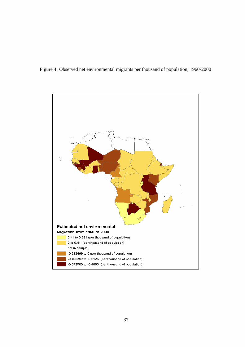
Figure 4: Observed net environmental migrants per thousandof population, 1960-2000

37

Figure 5: Predicted net environmental migrants per thousand of population, 2000-2099

38