A CGE Model for Tax Policy in Colombia

7/28/2019 A CGE Model for Tax Policy in Colombia

http://slidepdf.com/reader/full/a-cge-model-for-tax-policy-in-colombia 1/66

República de ColombiaDepartamento Nacional de Planeación

Dirección de Estudios Económicos

ARCHIVOS DE ECONOMÍA

A dynami c general equil i bri um model for t ax pol i cy

anal ysi s i n Colombi a

Thomas F. RUTHERFORDMiles K. LIGHTGustavo Adolfo HERNANDEZ

Documento 18915 de Mayo de 2002

La serie ARCHIVOS DE ECONOMIA es un medio de la Dirección de Estudios Económicos, no es un órganooficial del Departamento Nacional de Planeación. Sus documentos son de carácter provisional, deresponsabilidad exclusiva de sus autores y sus contenidos no comprometen a la institución.



A Dynamic General Equilibrium Model for

Tax Policy Analysis in Colombia

Thomas F. Rutherford and Miles K. LightEconomics Department

University of Colorado

Gustavo Hernandez∗

National Department of Planning

May 10, 2002

Abstract

The paper documents a dynamic general equilibrium model for Colombiabased on national accounts from 1999. The paper is part of a project in-tended to develop a capacity for the the design, specification, and applicationof computable models within the Colombian Ministry of Finance and Depart-ment of National Planning. Our analytical framework includes both forward-looking expectations and Harris-Todaro labor markets. In the present paperwe compare numerical results from the dynamic model with simpler static andsteady-state formulations to highlight the importance of transitional effectsin evaluating tax policy reform. Our applications include measurement of themarginal cost of funds from different tax bases and the evaluation of discretechanges in tariff structure. The structure of the labor and intermediate credit

markets have important implications for the ranking alternative tax reformproposals.

∗The authors would like to thank Sergio Prada and Juan Mauricio Ramırez from Ministry of Finance and Andres Escobar, and Omer Ozak from National Department of Planning for a numberof helpful comments. This is a working paper for discussion, the views expressed in this paper arethose of the authors and not necessarily those of the Ministry of Finance and National Departmentof Planning.



1 Introduction

This paper introduces a multi-sectoral, dynamic general equilibrium model for taxpolicy analysis in Colombia. The model incorporates Harris-Todaro migration and

unemployment and two alternative representations of international capital flows,

issues which are important considerations for tax reform in developing countries such

as Colombia. While the analysis presented in the paper provides policy-relevant

insights, the primary objective of the paper is pedagogic. We have developed a

template model which can provide a starting point for a variety of future studies of

the Colombian tax system.

There are two illustrative calculations reported in this paper. The first compares

the marginal cost of funds (MCF) from Colombia’s major tax streams. Here we find

that one peso of public funds costs 1.2 to 5 or more pesos of foregone current and

future consumption, depending on the tax instrument used to raise the revenue,

the time horizon of the model, and the labor market formulation. In a second set

of illustrative calculations we evaluate two alternative tariff-reform policies. The

first policy provides tariff exemptions for capital- and high-tech imports which is

intended to foster capital accumulation while the second moves toward a more uni-

form tariff structure, lowering tariff rates on some goods and raising rates on others.

In a second best context, economic theory does not indicate which of these policies

would be preferred, but our computable framework indicates that a movement to-

ward uniformity presents substantial efficiency gains while the movement away from

uniformity results in a loss of efficiency and fails to promote growth.

We do not put forward these policies as a particular tax reform agenda. Our

intent is only to illustrate how the model might be applied to evaluate specific

tax reforms. We leave future applications of the modeling framework to specific

tax proposals to our colleagues in the Ministry of Finance and the Department of

National Planning.

In order to highlight the role of the intertemporal margin on capital taxes, we

compare the results from the forward-looking dynamic model with the same policy

experiment analyzed in the context of the static and steady-state models.1 The

1See Rutherford and Tarr [2001] for a similar analysis for Chile of the differences between policy

conclusions based on static and dynamic models.

1



dynamic model tracks a transition between the short and long-run equilibria. For

many experiments, the cost of a distortionary tax policy is larger in a dynamic

model than a static model because capital accumulation increases the distortionaryeffect. Conversely, the transitional impacts are typically smaller than in a steady-

state model because the framework accounts for the cost of capital accumulation,

while this is only partially accounted for in the steady-state model.

We work in the framework of a classical Ramsey analysis of optimal economic

growth with perfect foresight. This is a natural starting point because of the generic

representation of financial markets. The model represents an open economy with

perfect competition in all markets, a representative consumer, and a constant rate

of technological progress. The underlying theoretical model is well studied in the

economics literature.2 This model is intended to provide a starting point for future

quantitative policy analysis, and we therefore have made a number of simplifying

assumptions to maintain transparency.

This paper compares results from a collection of related yet distinct models, it

is helpful to lay out the logical framework in some detail so that the similarities

and differences in model structure are readily apparent. We therefore begin with a

schematic overview of the equilibrium structure and benchmark data for the static

model.3 Thereafter we lay out the equations which characterize the steady-state and

dynamic extensions of the static model. After going through the model formulations,we consider two illustrative applications of the model for policy analysis. Appendices

are provided which cover programming details related to the implementation of

dynamic models in GAMS/MPSGE and instructions for running the model.

2See, for example, Blanchard and Fischer [1989], and Barro and Sala-i Martin [1995]. The

numerical representation of this model is less common in textbooks. See Lau et al. [2002] for an

introduction to dynamic equilibrium modeling in a complementarity format. Harrison et al., eds

[2000] contains a collection of papers based on policy-oriented dynamic general equilibrium model-

ing. The present analysis does not address the connection between tariff reform and productivity

growth as in Rutherford and Tarr [2002], but such an extension of the present model could be quite

useful.3Algebraic details of the static model are presented in Rutherford and Light [2002]

2



2 The Static and Steady-State Models

The static model for Colombia represents an Arrow-Debreu economy with constantreturns-to-scale and perfect competition. The model is based on 1999 Colombian

national accounts which distinguish 16 industries, government, and a single repre-

sentative household. Equilibrium in this model is characterized by a set of prices

and levels of production in each industry such that the market demand equals sup-

ply for all commodities. Producers are assumed to maximize profits, there is free

entry, and production exhibits constant returns to scale, hence no activity earns a

positive economic profit at equilibrium prices. Following Mathiesen (1985) we for-

mulate and solve as a complementarity problem in which three types of equations

define an equilibrium: market clearance, zero profit, and income balance.

The relationship between different blocks of a typical model is shown in Figure 1.

Taxes are discussed in the next section and therefore, for simplicity, do not appear

in this figure.

E i

TROW

T

M i

Y i

DiA ji

RA

G I C

'

E

c

'

T

'

r r r r r r r r r

t t

t t

¡ ¡

¡ ¡ !

c c c

K, LF , LI , N

Fig. 1. Flows in a static model

Sector’s i output (denoted Y i) is produced using capital K i, formal labor LF i ,

informal labor LI i , land N , and intermediate inputs described by A ji , an aggregate

3



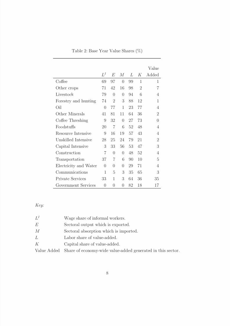
of domestic goods D j and imports M j. This same composite good enters private

consumption C , government consumption G, and investment I . Output from Y i

includes Di and E i. A representative agent RA represents a collective decisionprocess for allocating income to households and to a government. The representative

agent has an endowment of capital K , two types of labor (LF and LI ) and tax

revenue (not shown). The same consumer demands C, I and G.

Production sector Y i produces two types of commodities: domestic goods Di

and goods for export E i. These goods are assumed to be imperfect substitutes,

produced with a constant elasticity of transformation. For production, each sector

uses capital, labor, land and intermediate goods. As such, the sector’s i production

function is

Y i = g(Di, E i) = f (K i, LI i , LF

i , N i, A ji) (1)

where g is a constant-elasticity-of-transformation function for outputs, and f is a

nested Leontief - Cobb-Douglas production function for inputs. Capital, labor and

land enter as a Cobb-Douglas value-added aggregate. Intermediate inputs and the

value-added composite enter as a Leontief aggregate at the top level.

The representative consumer demands investment, private and government goods,

and receives transfers from the government. In the static model investment is ex-

ogenous, while private demand is determined by utility-maximizing behavior. (Con-

sumer utility consists of a Cobb-Douglas utility index defined over Armington ag-

gregations of domestic and imported commodities.) In the static model investment

is exogenously fixed. In all the models, the level of public provision is held constant,

and all tax policy analysis is undertaken subject to an equal yield constraint. When

one tax rate is reduced, another tax flow is increased to compensate for the lost

revenue.

Figure 2 provides an overview of the static model structure in which σ signifies

an elasticity of substitution and η is the elasticity of transformation.

4



K LF LI N

v v

v

d d

d

A1 ... A j

v v

v

d d

d 3 3 3 3 3

Y i

3 3 3 3 3

E i Di M i

T

row

Ai

T

row

3 3 3 3 3

E

T

C,G,I

σ = 1 σ = 0

σ = 0

η = 4

σ = 4

cRA

T T T T

Fig. 2. Structure of the static model

Table 1 presents a perspective on the sectoral shares of economic activity in 1999.

Here we see that as in many developing countries, GDP is generated primarily in

agriculture, resource-intensive and and service sectors. High tech / capital intensive

manufacturing accounts for only 3% of value-added but 57% of imports. The key

exports in 1999 were agricultural goods plus coffee (25% of export earnings) and oil

(22%). Over half of formal labor is employed in service sectors, a third of which is

in the public sector. Informal labor is largely employed in agricultural sectors (40%)and private service sector (45%).

The input-output data indicate that capital formation is based on inputs of con-

struction services and high technology/capital-intensive manufactured goods. Final

demand is composed of services (33%), foodstuffs (19%) and various manufactured

goods (27%).

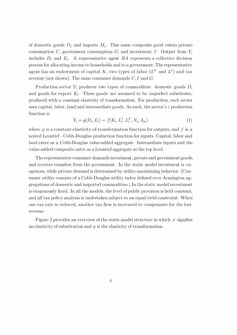
Table 2 describes the primary factor and trade content of various sectors in the

economy. Informal labor earns a relatively large share of aggregate wage payments

in agricultural sectors which are highly export-oriented. For example, 69% of wagepayments in the coffee sector are to informal workers, and 97% of coffee output is

exported.

When we look at trade exposure, we see a few highly export-oriented sectors

including oil (77%), other minerals (81%), and coffee (97%). Export shares for

manufactured goods range from 16 to 33%, while service sector goods are largely

5



untraded.

The capital value share column indicates the relative importance of capital in

the oil sector (77%) and for selected services (electricity is 71%, communications

65%). The manufactured goods have capital value shares ranging from 20 to 50%.

In the model implementation we include the option to distinguish base year

capital earnings between returns to physical capital and returns to sector-specific

resources. For example, it would not be appropriate to assume that all capital

earnings in the oil sector necessarily accrue to physical capital, otherwise we would

be assuming that an expansion of the sector only would require additional oil wells

and not new oil fields on which to place the wells. The scenarios described here do

not utilize this feature.Tables 3 and 4 describe the structure of direct and indirect taxes. Table 3 fo-

cuses on sectoral tax rates as they apply to value-added, output and inputs. The

term “VAT” is used somewhat loosely, as the model and actual application of this

tax is on agggregate demand rather than on sectoral value-added. While the posted

value-added tax rate is 16%, the base year data suggest that the VAT tax is applied

primarily on manufactured goods and communication services. Agricultural prod-

ucts, oil and most services are exempt, yet (as indicated in Table 4), this tax base

contributed nearly half of all indirect tax revenues in 1999.

Excise taxes apply on the value of production, both on sales in the domestic

economy and on exports. Excise taxes apply at the highest rate on natural resource-

intensive manufactures (15%) and coffee (11%). Looking at tax revenue (Table 4),

we find that given the relative size of sectors, the single most important indirect

tax in the economy is the excise tax on natural resource intensive production, a tax

which generated 2.6 billion pesos in 1999.

In 1999 tariffs were applied at a 5% rate on manufactured goods imports and

16% on agricultural goods. In terms of collected revenue, the tariff instrument

contributes a relatively small amount, only 11% of all indirect tax revenue.

There are direct taxes in Colombia. The nominal labor income tax is 17%, and

the nominal tax on capital gains is 32%. Our base year data indicate, however that

the collected rate on formal labor is 4% and the effective capital tax rate is 16%. In

the model we assume that informal labor is untaxed.

6



Table 1: Shares of Economy-Wide Totals (%)

ValueAdded LF LI K E M G I C

Coffee 1 1 4 0 8 0 0 -2 0

Othercrops 7 4 18 0 17 5 0 5 4

Livestock 4 1 13 1 0 0 0 4 1

Forestry and fishing 1 0 2 0 0 0 0 3 0

Oil 4 2 0 5 22 0 0 0 0

OtherMinerals 2 1 3 1 9 0 0 0 0

CoffeeThreshing 0 0 0 0 1 0 0 2 0

Foodstuffs 4 3 3 6 5 4 0 4 19

Natural Resources 4 5 1 3 10 14 0 3 10

Unskilled Intensive 2 3 2 2 7 9 0 4 9

Capital and High Tech 3 3 0 4 14 57 0 29 8

Construction 4 4 1 8 0 0 0 43 0

Transportation 5 7 8 2 3 3 0 0 8

Electricity, Gas, Water 4 3 0 9 0 0 0 0 3

Communications 3 3 0 7 1 1 0 0 4

Private Services 35 27 45 42 1 6 0 6 33

Government Services 17 33 0 10 0 0 100 0 2

Key:

Value Added Value Added generated in this sector

LF Formal labor

LI Informal labor

K Capital earningsE Exports

M Imports

G Aggregate public expenditure

I Investment demand

C Final consumption demand

7



Table 2: Base Year Value Shares (%)

Value

LI E M L K Added

Coffee 69 97 0 99 1 1

Other crops 71 42 16 98 2 7

Livestock 79 0 0 94 6 4

Forestry and hunting 74 2 3 88 12 1

Oil 0 77 1 23 77 4

Other Minerals 41 81 11 64 36 2Coffee Threshing 9 32 0 27 73 0

Foodstuffs 20 7 6 52 48 4

Resource Intensive 9 16 19 57 43 4

Unskilled Intensive 28 25 24 79 21 2

Capital Intensive 3 33 56 53 47 3

Construction 7 0 0 48 52 4

Transportation 37 7 6 90 10 5

Electricity and Water 0 0 0 29 71 4

Communications 1 5 3 35 65 3Private Services 33 1 3 64 36 35

Government Services 0 0 0 82 18 17

Key:

LI Wage share of informal workers.

E Sectoral output which is exported.

M Sectoral absorption which is imported.

L Labor share of value-added.

K Capital share of value-added.

Value Added Share of economy-wide value-added generated in this sector.

8



Table 3: Benchmark Tax Rates (%)

vat ty tm

Coffee 0 11 0

Othercrops 0 0 16

Livestock 0 0 2

Forestryfishing and hunting 0 0 5

Oil 0 2 0

OtherMinerals 0 0 3CoffeeThreshing 0 1 0

Foodstuffs 0 2 7

NaturalResources Intensive Industries 6 15 5

UnskilledLabor Intensive Industries 8 2 5

Capitaland High Technology Industries 6 2 5

Construction 0 1 0

Transportation 1 1 0

Communications 15 2 0

Private Services 2 1 1Government Services 0 1 0

Key:

vat “Value-added tax” applies to all sales of

domestic and imported goods .

ty Excise tax applies to sectoral output (both

domestic sales and exports).

tm Import tariff.

9



Table 4: Tax Revenue

vat ty tm Total %

Coffee 0 0.26 0 0.26 2

Other crops 0 0 0.21 0.22 2

Livestock 0 0 0 0 0

Forestry fishing and hunting 0 0 0 0 0

Oil 0 0.12 0 0.12 1

Other Minerals 0 0.01 0 0.01 0

Coffee Threshing 0 0.01 0 0.01 0

Foodstuffs 0.12 0.34 0.09 0.55 4

Natural Resources Intensive Industries 1.41 2.60 0.21 4.21 31

Unskilled Labor Intensive Industries 0.96 0.19 0.14 1.28 9

Capital and High Technology Industries 1.95 0.26 0.82 3.03 22

Construction 0 0.15 0 0.15 1

Transportation 0.07 0.18 0 0.25 2

Electricity Gas and Water 0 0.04 0 0.04 0

Communications 1.06 0.13 0 1.19 9

Private Services 1.00 0.93 0.01 1.93 14

Government Services 0 0.40 0 0.40 3

Total Indirect Revenues 6.56 5.61 1.49 13.66

% 48 41 11 100

Labor Tax Revenues 2.23

Capital Tax Revenues 6.95

Billions of 1999 Colombian Pesos.

10



2.1 The Steady-State Model

The steady-state model evaluates the long-run impact of a policy change after in-vestment and capital stock have fully adjusted. We assume that for a given rate of

return and cost of investment, the capital stock is initially optimal. After a policy

reform, the model is based on the presumption that investment and capital stocks

readjust to a level which re-equalibrates the present value earnings of a unit of new

capital and the cost of a unit of new capital (Tobin’s q , the ratio of market value

to replacement cost, is equal to unity). For example, a trade reform may lead to

a new equilibrium in which the rate of return on capital increases relative to the

cost of investment. This implies that in a dynamic sense, a fixed capital stock is

no longer optimal for the new equilibrium – investment should be forthcoming untilthe marginal productivity of capital is reduced to the long run equilibrium where

the rate of return on capital is again proportional to the cost of capital.

In a comparative static model we allow the price of capital to vary while holding

constant the aggregate stock of capital. The steady-state calculation essentially re-

verses this: we allow the capital stock (and investment demand) to be endogenously

determined while holding constant the price of capital (see Hansen and Koopmans

[1972] and Dantzig and Manne [1974]).

Since the steady-state calculation ignores the forgone consumption required tomove from the initial capital stock to the new steady-state level, in policy experi-

ments which foster capital accumulation this calculation provides an upper bound

on potential welfare gains in a long run classical Solow type growth model. This ap-

proach to steady-state evaluation in a multi-regional trade model was implemented

in Harrison et al. [1996] and has also been used by Francois et al. [1997].

The steady-state equilibrium is characterized by the static model with an ad-

ditional variable which represents the equilibrium size of the capital stock. In the

benchmark equilibrium, total capital and capital returns are fixed. In the steady-

state, κ alters the endowment of physical capital: 4

i

K i = κK,

4Table 5 provides definitions for the symbols used in this and the subsequent section of the

paper.

11



and investment demand is scaled proportionally:

Ai = j X

d

ij + C + G + κa

I

i

¯I.

Both of these effects enter into the representative consumer’s budget constraint:

max U (C )

s.t.

κ rK K + wI Li + wF LF +

i pN i N i + T =

i pi C i + κpI I

Let pI represent the marginal cost of a unit of new investment. In our model this

cost function has the form:

pI =

i

aI i pi

In the steady-state, capital stock adjusts so that the ratio of the rental rate on

capital to the cost of producing a unit of the capital good is constant:

rK

pI = r + δ

implying that in the long-run equilibrium, the return to capital is equal to the sum

of the discount rate on future consumption plus depreciation.

2.2 Labor Markets

The base model assumes: (i) labor taxes apply only to formal sector employment,

(ii) there is unemployment in the formal sector associated with downward rigidity of

the wage rate, and (iii) migration between the formal and informal sectors is driven

by both a wage differential and the formal-sector unemployment rate as it affects the

probability of an informal worker finding a job in the formal sector, and (iv) labor

is measured in the model in efficiency units – in the social accounting framework

the labor input is the wage bill, which represents wages plus benefits. We do not

attempt to account for differences in per-capita wages across sectors.

The following sets of equations apply in every period t. for notational simplicity

the t subscript is surpressed.

12



The formal-sector unemployment rate is determined by a wage equation , in which

a wage elasticity parameter, θ, relates the wage rate to the unemployment rate:

wF

pC = φu−1/θ. (2)

In this expression wF is the formal sector wage rate, pC denotes a consumer goods

price index and u is the formal sector unemployment rate , equal to 16% in 1999. In

specifying this model θ is specified exogenously, and φ is calibrated to match the

base year data.

This type of wage equation can be derived from trade union or efficiency wage

models (see Hutton and Ruocco [1999]). In our calculations we investigate two

alternative specifications of this wage equation, one in which θ = 1 and a second inwhich θ = ∞.

Following Todaro [1969], we link the formal-informal labor migration rate to

the real-wage differential and the rate of unemployment. Migration occurs when

the expected real wage for formal employment increases relative to the informal

wage. Workers migrate into the formal labor sector until informal wages are equal

to expected formal wages:

wI = (1 − u) · wF (3)

Labor supply for the formal and informal sectors is determined by the migrationrate and the unemployment rate. First, the supply of formal labor is equal to the

employed fraction of the workers who chose to migrate to the formal sector:

LF = (1 − u) m L (4)

where m is the migration rate between the informal and formal labor sectors, and

L is the total workforce. Then the informal labor supply is equal to those workers

who did not migrate:

LI = L(1 − m) (5)

When θ = ∞, the formal sector wage is fixed. In addition to the θ = 1 andθ = ∞ variants of the wage-curve model, we also investigate a flexible wage model

in which aggregate employment of formal and informal workers are exogenous and

the associated wages adjust to clear each market. The flexible wage model assumes

no induced changes in the formal or informal sector unemployment rate as a result

of policy measures.

13



Table 5: Notation for Static and Steady-State Models

Static Model:

i Sectoral identifier

Di Domestic output

E i Exports

K i Capital stock

LF i Formal labor

LI i Informal labor

Aij Intermediate demand

Y i Aggregate output

C i Private demand for ith good

I i Investment demand

Gi Government demand

Steady-State Model:

K Aggregate Capital Stock

κ Capital stock level in steady-state equilibrium(κ = 1 in the base year)

I Aggregate base-year investment

aI i Capital formation coefficient - units of good i per

unit of aggregate investment (I i = κaI i I )

rk Rental price on physical capital

wI , wF Formal and Informal wage (net of tax)

pN i , N i Price and supply of sector i-specific resources

pi Price of a unit of new investment

ρ Steady-state interest rateδ Steady-state depreciation rate

pC Aggregate consumption price index

u Unemployment rate

u(·) Instantaneous utility factor

θ Formal sector wage-unemployment elasticity

φ Wage-curve scale factor

14



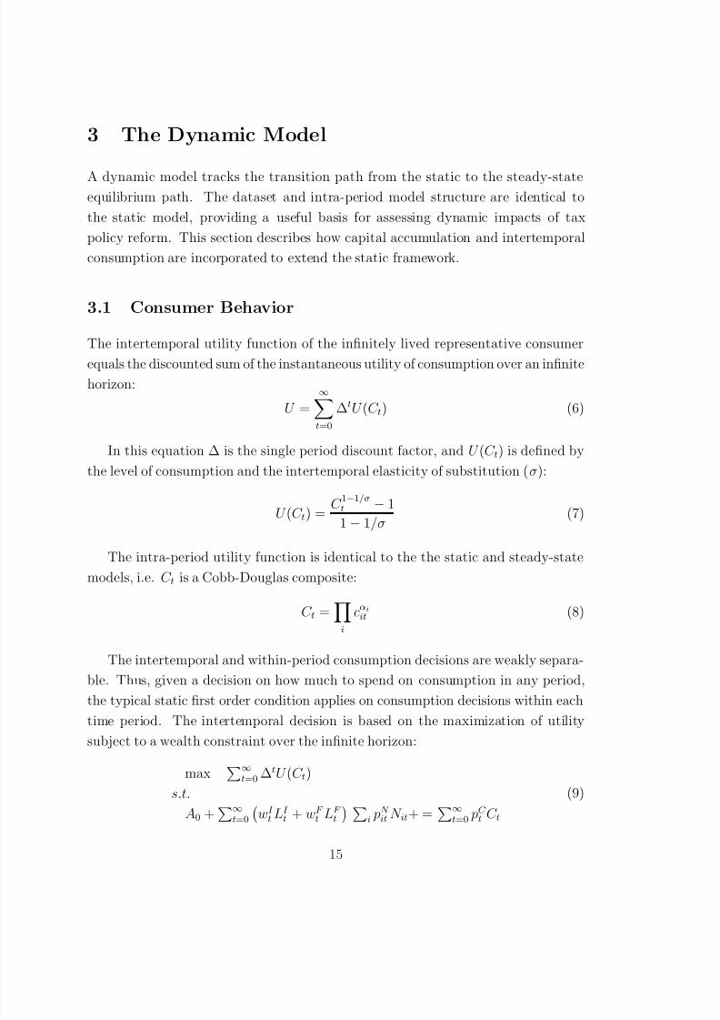
3 The Dynamic Model

A dynamic model tracks the transition path from the static to the steady-stateequilibrium path. The dataset and intra-period model structure are identical to

the static model, providing a useful basis for assessing dynamic impacts of tax

policy reform. This section describes how capital accumulation and intertemporal

consumption are incorporated to extend the static framework.

3.1 Consumer Behavior

The intertemporal utility function of the infinitely lived representative consumer

equals the discounted sum of the instantaneous utility of consumption over an infinite

horizon:

U =∞

t=0

∆tU (C t) (6)

In this equation ∆ is the single period discount factor, and U (C t) is defined by

the level of consumption and the intertemporal elasticity of substitution (σ):

U (C t) =C 1−1/σt − 1

1 − 1/σ(7)

The intra-period utility function is identical to the the static and steady-state

models, i.e. C t is a Cobb-Douglas composite:

C t =

i

cαi

it (8)

The intertemporal and within-period consumption decisions are weakly separa-

ble. Thus, given a decision on how much to spend on consumption in any period,

the typical static first order condition applies on consumption decisions within each

time period. The intertemporal decision is based on the maximization of utility

subject to a wealth constraint over the infinite horizon:

max∞

t=0 ∆tU (C t)

s.t.

A0 +∞

t=0

wI t LI

t + wF t LF

t

i pN it N it+ =

∞

t=0 pC t C t

(9)

15



The budget constraint contains the value of the initial asset holdings, A0. This

includes the value of the base year capital stock, pK 0 K 0, as well as the net value of

asset holdings outside the country. All prices in the budget constraint are definedin present value terms, discounted to period 0 (1999). The present value of wealth

includes the value of the entering (period 0) capital stock, the value of sector-specific

resource rents, the present value of (formal and informal) wage income and all other

taxes and transfers.

3.2 Baseline Growth Path

In order to calibrate the dynamic model, we assume that the economy is initially on

the steady-state growth path. This allows us to describe the evolution of capital and

labor. A steady-state is defined as a situation in which all quantity variables grow at

a constant rate, g and all present-value prices decline with a constant interest rate,

r. In this model labor, capital and sector-specific resources are assumed to grow at

a constant rate g:

Lt = L(1 + g)t, (10)

N it = N i(1 + g)t, (11)

and the capital evolves through geometric depreciation

K t+1 = (1 − δ )K t + I t = K t (1 + g) (12)

where I t is investment and δ is the depreciation rate.

Equation (3.2) implies that on the steady-state growth path I t = (g + δ )K t.

Investment takes place at a level which covers growth plus depreciation.

When relative factor prices are constant, output for each sector also grows at the

same rate g:

Y it = Y i(1 + g)t (13)

All future prices (including the price of labor and capital) in terms of present

value are:

pi,t+1 =pit

1 + r(14)

16



3.3 Capital Accumulation

In our dynamic equilibrium framework, there are two prices for capital. p

K

t is thepurchase price for new capital, and rK

t is the rental price for capital. Total capital

returns for a given period, V K t are equal to the capital stock times the capital rental

rate:

V K t = K t · rK

t . (15)

Capital markets are assumed to operate competitively which implies that the

period t purchase price for capital equals the period t rental earnings plus the value

of the remaining capital sold in the subsequent period:

pK t = rK t + (1 − δ ) pK t+1. (16)

The Euler condition equates the marginal utility of consumption and investment.

It implies that the capital purchase price equals 1 + r times the current cost of

consumption.

pK t = pI t−1 = (1 + r) pI t . (17)

Substitution of pK t from equation (17) for pK

t+1 into (16) defines prices over time.

The rental price is for capital in terms of the cost of investment is:

rK t = (δ + r) pI t (18)

This equation states that the steady-state rental price of capital equals the cost of

interest and depreciation.

If we observe initial returns to capital as V K from the social accounts for 1999,

then the initial level of investment which is consistent with these returns should be:

I 0 =δ + g

δ + rV K 0 . (19)

The 1999 social accounts for Colombia report capital returns and investmentas shown in Table 6. This indicates that the base year data are inconsistent with

a balanced growth path. At this point, one could compute a baseline equilibrium

growth path, based on assumptions about future developments in productivity and

the transition to a steady state after a given number of years. In order to avoid

the complication of collecting baseline growth-path forecasts, in the present analysis

17



Table 6: 1999 Capital Returns and Investment for Colombia

Private Public Combined

Investment Demand 21.1 - 21.1

Adjusted Investment Demand 25.3 - 25.3

Capital Receipts (V K ) 30.4 3.2 33.7

we have instead chosen to adjust the base year value shares in order to impose a

steady-state growth path. This approach is advisable during the initial stages of

model development in order to simplify testing the model for logical consistency.

We leave the construction of a baseline forecast to future model development work.

When adjusting the base year social accounts to achieve steady-state consistency,

there are several degrees of freedom in the computation of an aggregate capital

stock. The capital stock can be computed based upon either the capital earnings or

investment. If we evaluate the capital stock on the basis of returns, with an assumed

5% interest rate and a 7% depreciation rate we find:

K 0 =V K

r + δ =

(30.4 + 3.2)

0.05 + 0.07= 280.7

Accordingly, the steady-state investment level is calculated as:

I 0 = (g + δ ) K 0 = 25.3

In the base-year data we find I 1999 = 21.1, a value nearly 20% lower than that

implied under the steady-state assumptions. The fact that 1999 investment is below

the steady-state level suggests that the economy-wide capital stock is above the

steady-state level. This seems implausible and leads us to conclude that future

model development should more carefully examine the capital earnings data in the

social accounts. In Input-Output data, capital returns are often computed as a

residual and can deviate substantially from the long-run value shares. We have

therefore adjusted investment by solving a least-squares reallocation of investment

and consumption demands, subject to the constraint that aggregate investment

equals 25.3.

18



3.4 Financial Capital Flows

An open economy with unrestricted borrowing is characterized by equalization of the domestic and international interest rates. In many countries, this is a coun-

terfactual assumption. In the present model, we explore the role of international

financial capital mobility by implementing two alternative representations of the

current account constraint.

In the “Balance of Payments” model, the real exchange rate is computed within

each period and adjusts to equalize the value of exports and imports in that year.

That is:

i

¯ pX it X it(µt) =

i

¯ pM it M it(µt)

where ¯ pX it and ¯ pM it are the international prices of imports and exports, X it and M it

are the trade volumes, and µt is the real exchange rate in period t. In this model

the domestic interest rate is endogenous, rDt = µt+1/µt − 1.

The “Capital Flows” model allows for net changes to the balance of payments

accounts within each period. A single, infinite-horizon intertemporal budget replaces

the period-by-period constraints:

∞

t=0i

¯ pX it X it(µt) =∞

t=0i

¯ pM it M it(µt) = 0 (20)

and the time path of the real exchange rate is determined by the international

interest rate:

µt+1 =µt

1 + r(21)

In the open capital markets model the real exchange rate may adjust only in period

0 following a policy shock.

In the T -period model, the intertemporal trade balance is written:

T

t=0

i

¯ pX it X it(µt) − ¯ pM

it M it(µt)

= AT +1 − pK T +1K T +1 (22)

where AT +1 is the level of terminal assets and K T +1 is the terminal capital stock,

both of which are approximated as described in the subsequent section.

19



3.5 Approximating an Infinite Horizon

Approximation of infinite horizon equilibria in this model follows the strategy pro-posed by Lau et al. [2002]. At an intuitive level, there are two issues in the ap-

proximation method. First, we need to choose a terminal (period T + 1) capital

stock which is consistent with smooth growth in investment in the final periods of

the model (state variable targeting ). Second, we need to determine an estimate of

terminal assets which is consistent budget balance and steady-state growth from

period T onwards. The terminal asset approximation decomposes the consumer

choice problem for the infinitely-lived agent into one choice problem for periods 0 to

T , and a second problem from period T + 1 to ∞. An assumption of steady-state

growth permits us to solve for period T + 1 assets using the budget constraint forthe post-terminal utility maximization problem.5

Algebraically, the terminal capital stock is determined through two equations.

The first is a simple capital stock evolution equation applied to the post-terminal

year:

K T +1 = (1 − δ )K T + I T (23)

This constraint is associated with a price variable pK T +1 which rewards investment

and depreciated capital carried over to the post-terminal year. The second con-

straint selects the value of K T +1 at a level which assures steady-state growth in theassociated control variable in the terminal period:

I T = (1 + g)I T −1 (24)

This equation replaces the zero profit condition (16) which is associated with capital

stocks in the earlier periods of the model.6

5The determination of a reasonable value of T is based on numerical experimentation. We felt

that for the experiments reported in this paper, a 60 year horizon provides a reasonable trade-off

between run time and numerical precision. The dynamic model solves in about 5 minutes on a 1.8

GHz PC with an asset approximation error of less than 0.2%.6Equation (24) represents a primal termination condition . An alternative approach which may

sometimes provide better results is a dual termination condition , such as: pK T +1 =pKT

1+r. This

adjusts the terminal capital stock to a level such that the capital price is moving on it steady-state

growth path between periods T and T + 1. When T is sufficiently long, the model results are

virtually identical for either approach.

20



In a model with international capital flows, the terminal assets of the household

need not equal the value of the domestic capital stock, even if these values are equal

in the initial year of the model. In order to understand our method of calculatingterminal assets, it is helpful to think of the consumer utility maximization problem

as two separate optimizations which are linked through the period T + 1 assets:

maxT

t=0 ∆tU (C t)

s.t.

A0 +T

t=0

i pN it N it + wI

t LI t + wF

t LF t

=T

t=0 pC t C t + AT +1

(25)

andmax

∞

t=T +1 ∆tU (C t)

s.t.AT +1 +

∞

t=T +1

i pN it N it + wI

t LI t + wF

t LF t

=∞

t=T +1 pC t C t(26)

Separability of the intertemporal utility means that when AT +1 is chosen at the op-

timal value for the ∞-horizon program, then the two subproblems together produce

a consumption path which is identical to the infinite horizon program.

Suppose that T is chosen to be sufficiently long that the economy is virtually

in the steady-state growth path from T + 1 onwards. In this case we can use the

budget constraint from equation (26) to approximate AT +1:

AT +1 =∞

t=T +1

i pC t C t −

i p

N it N it − w

I t L

I t − w

F t L

F t

≈ pC T C T −

i pN iT N iT − wI

T LI T + wF

T LF T

1+gr−g

(27)

Using a complementarity format permits us to include this constraint in the

T -horizon model to simultaneously compute the transition path and determine the

terminal asset position.7

7We do several calculations in the following with an equal yield public sector budget constraint.

In these experiments, there is an immediate and permanent change in some set of taxes and we

calculate the level of a replacement tax such that the present value of tax revenue over an infinitehorizon remains unchanged. For these calculations we use a terminal asset equation for the public

sector analogous to the household asset calculation in order to compute changes in tax revenue

over the infinite-horizon, including changes induced in year T + 1 and thereafter:

AGT +1 ≈

pGT GT − T LT − T K T − T Y T − T M

T − T vatT

1 + g

r − g,

in which the T kt denotes tax revenue from instrument k ∈ {L,K,Y,M,V AT } in period t.

21



4 Illustrative Applications

We present two sample applications. In the first we estimate the marginal cost of funds (MCF) under alternative model specifications. The objective of this exer-

cise is develop an understanding for the relative importance of labor market and

intertemporal features for the MCF. As a second sample application of the model

we evaluate a seemingly beneficial proposal to reduce tariffs on High Tech/Capital

intensive imports, goods which represent a large share of new investment. The log-

ical appeal of such a policy is that it could promote growth through lowering the

cost of capital formation. While the policy proposal seems reasonable and logical,

the model reveals that the reasoning is flawed. The numerical model shows that an

exemption of tariffs on this sector generates a substantial welfare loss rather than again. As an alternative reform, we consider the economic effect of applying a uni-

form tariff and we find under a wide range of assumptions that this could provide a

substantial improvement in growth and welfare.

4.1 The Marginal Cost of Funds

The marginal cost of funds is a computed value which approximates the efficiency

cost of increasing public expenditure. This is computed by making a small increase

in tax rates and assessing the resulting changes in tax revenue and consumer welfare.

We do this calculation in the static, steady-state and dynamic models in order to

evaluate the importance of the intertemporal margin. In this analysis, we compare

the cost of tax revenue from each of five major revenue sources, ty, tm,vat,tl, and tk.

(See Tables 3 and 4 for the rates and revenue contributions from these tax bases.)

The marginal cost of funds computed in the static, steady-state, and dynamic

models are listed in Tables 7, 8 and 9. We calculate the MCF as the total dollar

change in Hicksian equivalent variation divided by the total dollar change in govern-

ment revenues, based on model calculations in which there is a marginal proportional increase in the tax base. In the dynamic model we use discounted present values

over an infinite horizon to measure both the EV and the change in tax revenue.

Intuitively, the MCF is higher in a the long-run model because capital is no longer

a fixed factor. Households have more options to substitute away from taxed goods,

22



which increases the distortion of a tax. This line of thought is generally consistent

with the “Ramsey rule” for optimal taxation [Ramsey 1928], which suggests that

taxes are more distortionary as the elasticity of demand increases.

We find that in spite of the labor market impacts, direct taxes on labor are a

relatively efficient source of additional revenues. One reason this may be the case

for Colombia is that existing effective taxes on labor income are low in our dataset

(around 4%).

While the wage tax is relatively efficient, we find that labor market imperfections

have a extremely important impact on the estimated MCF, potentially even greater

than the intertemporal margin. In the current set of calculations the rigid wage

model has an MCF ranging from 8 for the labor tax to infinity for the import tariff.8

What are we to conclude from these results?

1. Labor market imperfections could make public funds expensive in Colombia.

A more careful assessment of the empirical evidence and appropriate theory

which characterize labor markets in Colombia is required before we can assess

the MCF with any degree of precision. Empirical estimation of θ is useful and

relatively easy to do.

2. A conservative lower bound on the MCF for nearly any of the tax instruments

is around 1.5. This has important implications for cost-benefit analysis of

public projects in Colombia.

3. MCF estimates based on the static model provide a reasonable tight lower

bound on MCF estimates from a dynamic model, and MCF estimates for the

steady-state model provide a loose upper bound.

8In the rigid-wage, steady-state model, benchmark tariff rates are on the back side of the Laffer

curve. A marginal increase in τ M produces a net decrease in tax revenue.

23



Table 7: MCF Estimates from the Flexible Wage Model

static steady bopcon capflow

VAT 1.16 1.68 1.24 1.29

TY 1.57 1.78 1.48 1.51

TM 1.78 2.50 1.75 1.82

TL 1.16 1.28 1.11 1.12

TK 1.13 2.69 1.43 1.57

Table 8: MCF Estimates from the Wage Curve Model (θ = 1)


VAT 1.30 2.18 1.51 1.60

TY 1.83 2.23 1.78 1.83

TM 2.08 3.38 2.19 2.32

TL 1.38 1.68 1.37 1.40

TK 1.11 3.50 1.65 1.90

Table 9: MCF Estimates from the Rigid Wage Model (θ = ∞)


VAT 2.15 16.25 4.16 5.93

TY 4.12 18.78 5.51 7.24TM 5.16 ∞ 11.76 30.11

TL 2.81 8.10 3.86 4.63

TK 1.03 146.54 3.22 6.01

24



4.2 Evaluating a Tariff Reform Proposal

A common policy goal for developing countries is increased capital formation andGDP growth. Examining Table 2, it might seem that one means of encouraging

capital formation would be to lessen the tariff burden on goods which are used

intensively in investment. The base year statistics indicate that capital/high tech

goods (htc) comprise 29% of investment and 57% of htc supply was imported in

1999.

While the tariff rate on capital imports is only 5%, it seems (ex-ante) plausible

that eliminating this tariff might expand growth. The benefits of lowering this tax

must be considered in light of the costs related to raising revenues from other sources.

Tariff revenues from htc imports were 0.82 billion Colombian pesos in 1999, justover half of total tariff revenues.

When we compute the comparative dynamic growth path in the model with

free capital flows, we find that eliminating the htc nearly eliminates the domestic

htc industry, particularly when the tariff is replaced by an increase in value-added

taxes. Figure 1 indicates that there a slight positive impact on investment when

revenues are replaced using an excise or labor tax, but the net impact is negative

when the lost tariff reveue is recovered through value-added taxes. The degree to

which investment is adversely affected also depends on financial capital flows. Whenthere is unrestricted access to international credit markets, high-technology imports

are rapidly substituted for domestically produced htc goods. In the model with

period-by-period trade balance constraints, the decline of domestic htc production

takes place over many more years.

The tariff policy is shown to reduce the rate of domestic investment, but it is

not completely clear why investment falls. Figure 2 helps diagnose these results.

Here we have shown the absolute declines in capital demand for those sectors that

experience a fall in capital use. Here we see that htc itself is responsible for the

fall in investment: htc import competition drives down the demand for domestichtc, and this leads to a decrease in the htc demand for capital. The tariff makes

investment less expensive, but cripples the domestic industry which is most capital

intensive.

Figure 1 indicates that revenue recycling through the existing excise taxes or the

25



labor tax could lead to an increase in investment, yet Figure 3 shows that no matter

which replacement tax is applied, the tariff exemption for htc is welfare worsening.

The least adverse impact is in the balance of payments constrained case, where thebalance of payments constraint limits htc import substitution. This implies that it

takes time for the policy to have an adverse impact.

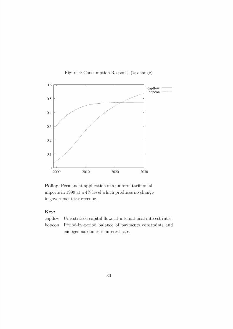
The final figure, Figure 4, indicates that a movement toward tariff uniformity

is more beneficial than piecemeal tariff exemptions. In this scenario, a uniform 4%

tariff achieves an equal yield with no change in other domestic taxes. These results

are consistent with findings from previous work in Chile [Harrison et al. 2002] as

well as the theoretical literature [Hatta 1977].

26



Figure 1: Investment Response (% change)

-2

-1.5

-1

-0.5

0

0.5

1

2000 2010 2020 2030

capflowbopcon

exciselabor

Policy: Permanent elimination of the tariff on high-

technology and capital-intensive goods in 1999.

Key:

capflow Unrestricted capital flows at international

interest rates. (revenue replacement:

VAT)

bopcon Period-by-period balance of payments con-

straints and endogenous domestic interest

rate. (Revenue replacement: VAT)

excise Unrestricted capital flows at internationalinterest rates. (Revenue replacement: TY)

labor Unrestricted capital flows at international

interest rates. (Revenue replacement: TL)

27



Figure 2: Change in Sectoral Capital Demand (%)

-0.5

-0.45

-0.4

-0.35

-0.3

-0.25

-0.2

-0.15

-0.1

-0.05

0

0.05

2000 2010 2020 2030

HTC

ELE

COM

SER



Key:

htc Capital and High Technology Industries

ele Electricity, Gas and Water

com Communications

ser Private Services

28



Figure 3: Consumption Response (% change)

-0.35

-0.3

-0.25

-0.2

-0.15

-0.1

-0.05

0

0.05

0.1

0.15

2000 2010 2020 2030

capflowbopcon

exciselabor



Key:

capflow Unrestricted capital flows at international

interest rates. (revenue replacement:

VAT)

bopcon Period-by-period balance of payments con-

straints and endogenous domestic interest

rate. (Revenue replacement: VAT)

excise Unrestricted capital flows at internationalinterest rates. (Revenue replacement: TY)

labor Unrestricted capital flows at international

interest rates. (Revenue replacement: TL)

29



Figure 4: Consumption Response (% change)

0

0.1

0.2

0.3

0.4

0.5

0.6

2000 2010 2020 2030

capflowbopcon

Policy: Permanent application of a uniform tariff on all

imports in 1999 at a 4% level which produces no change

in government tax revenue.

Key:

capflow Unrestricted capital flows at international interest rates.

bopcon Period-by-period balance of payments constraints and

endogenous domestic interest rate.

30



5 Conclusions

We use this section to reflect on aspects of the modeling work which are not empha-sized in the paper

Data Work Substantial effort and experience were leveraged to construct and

interpret the base year data for use with a CGE model. In many cases, this work is

far more difficult that the actual implementation of the model equations. Although

the present paper does not emphasize data issues, we caution the reader not to

discount the difficulty and importance of this type of work.

Tax Interpretation The representation of tax margins in the current analysis is

stylized. We have identified the key components of the direct and indirect taxes, but

we have not attempted to characterize differences between the average and marginal

rates nor have we considered the costs of collection or rates of evasion. Informed

adjustments of the tax margins could alter the MCF estimates and could conceivably

alter our policy analysis conclusions. More work is clearly warranted in this area.

Programming Details Model implementation issues have been only mentioned

in the appendices describing operational details. There are a number of subtleties in-volved in the implementation of multisectoral, dynamic general equilibrium models.

We rely heavily on the GAMS/MPSGE programming language for model specifica-

tion (see Rutherford [1999]) and the PATH solver (see Ferris and Munson [2000]).9

Use of GAMS/MPSGE greatly reduces the scope for programming errors, as we

avoid writing out cost functions, expenditure functions and demand functions. The

disadvantage of the MPSGE approach is that this makes the model less accessible

for economists who are unfamiliar with the syntax. It could be helpful to pro-

duce an algebraic implementation of the same model using GAMS/MCP, if only to

provide a transparent and comprehensive documentation of the model inputs and

assumptiosn.

9This is not a particularly large model for PATH. The transitional dynamic model with annual

time periods through 2060 involves roughly 5000 variables with a nonlinear system of equations

whose sparse Jacobian is 0.28% dense. A typical scenario solves on a PC in under a minute.

31



5.1 Further Research

We can envision a number of interesting directions in which the current model mightbe extended. We will list some of the ideas in random order:

Taxation and violence. The present model does not address the economic ef-

fects of sabotage and guerrilla activities which have severely disrupted a number of

important economic activities in the country. Future application of the model might

attempt to quantify the economic gains which could be realized through achieving

a lasting solution to the current civil unrest.

Property rights, idle capital and growth. de Soto [2001] provides an inter-

esting new perspectives on the role of property rights in the development process.

Our dynamic model incorporates forward-looking markets with price-responsive in-

vestment and could be calibrated to account for differences between the market and

private return to capital. It could be intriguing to see if the model might be extended

to quantify some of the market imperfections which DeSoto has emphasized.

International trade. The present model is based solely on national accounts for

Colombia and does not incorporate bilateral trade data. It would be interesting toextend the model to provide a tool for examining the economic effects of FTAA

accession or other regional trading agreements. A natural stragety for such an

extension would be to build on the GTAP dataset and framework.

Tax reform and poverty. There is a 1997 SAM which provides much more

sectoral and household detail. It would be quite interesting to investigate both

efficiency and equity using the household data from this source. Clearly, there is a

link between rural poverty and violence, and given the adverse impact of violence

on growth, there is a clear need for tools which can evaluate the distributional

consequences of tax reform.

32



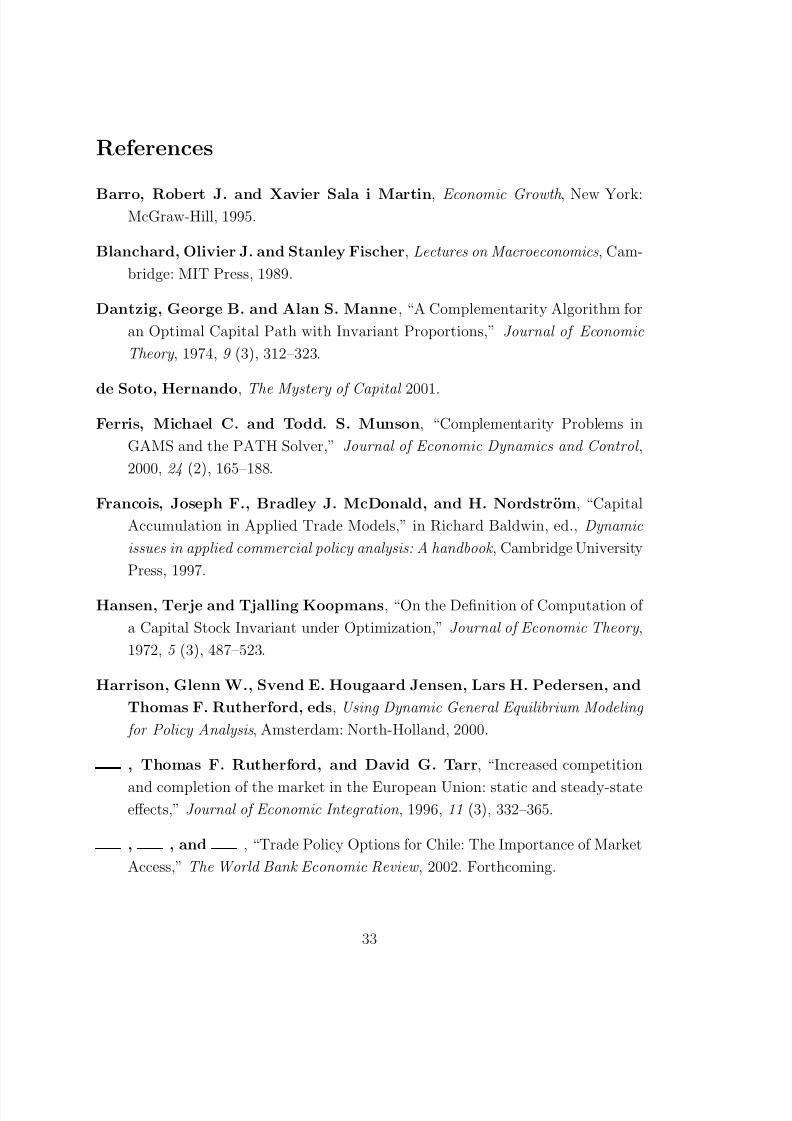
References

Barro, Robert J. and Xavier Sala i Martin, Economic Growth , New York:McGraw-Hill, 1995.

Blanchard, Olivier J. and Stanley Fischer, Lectures on Macroeconomics , Cam-

bridge: MIT Press, 1989.

Dantzig, George B. and Alan S. Manne, “A Complementarity Algorithm for

an Optimal Capital Path with Invariant Proportions,” Journal of Economic

Theory , 1974, 9 (3), 312–323.

de Soto, Hernando, The Mystery of Capital 2001.

Ferris, Michael C. and Todd. S. Munson, “Complementarity Problems in

GAMS and the PATH Solver,” Journal of Economic Dynamics and Control ,

2000, 24 (2), 165–188.

Francois, Joseph F., Bradley J. McDonald, and H. Nordstrom, “Capital

Accumulation in Applied Trade Models,” in Richard Baldwin, ed., Dynamic

issues in applied commercial policy analysis: A handbook , Cambridge University

Press, 1997.

Hansen, Terje and Tjalling Koopmans, “On the Definition of Computation of

a Capital Stock Invariant under Optimization,” Journal of Economic Theory ,

1972, 5 (3), 487–523.

Harrison, Glenn W., Svend E. Hougaard Jensen, Lars H. Pedersen, and

Thomas F. Rutherford, eds, Using Dynamic General Equilibrium Modeling

for Policy Analysis , Amsterdam: North-Holland, 2000.

, Thomas F. Rutherford, and David G. Tarr, “Increased competition

and completion of the market in the European Union: static and steady-stateeffects,” Journal of Economic Integration , 1996, 11 (3), 332–365.

, , and , “Trade Policy Options for Chile: The Importance of Market

Access,” The World Bank Economic Review , 2002. Forthcoming.

33



Hatta, Tatsua, “A Theory of Piecemeal Policy Recommendations,” Review of

Economic Studies , 1977, 44 (1), 1–21.

Hutton, J. and Anna Ruocco, “Tax Reform and Employment in Europe,” In-

ternational Tax and Public Finance , 1999, 6 , 263–288.

Lau, Morten I., Andreas Pahlke, and Thomas F. Rutherford, “Approxi-

mating infinite-horizon models in a complementarity format: a primer in dy-

namic general equilibrium analysis,” Journal of Economic Dynamics and Con-

trol , 2002, 26 , 577–609.

Ramsey, Frank, “A Mathematical Theory of Saving,” Economic Journal , 1928,

38 , 543–559.

Rutherford, Thomas F., “Applied General Equilibrium Modeling with MPSGE

as a GAMS Subsystem: An Overview of the Modeling Framework and Syntax,”

Computational Economics , 1999, 14, 1–46.

and David G. Tarr, “Regional Trading Arrangements for Chile: Do the

Results Differ with a Dynamic Model?,” Working Paper, The World Bank

2001.

and , “Trade liberalization, product variety and growth in a small openeconomy: a quantitative assessment,” Journal of International Economics ,

2002, 56 , 247–272.

and Miles K. Light, “A General Equilibrium Model for Tax Policy Analysis

in Colombia,” Working Paper 22, Department of National Planning 2002.

Todaro, Michael P., “A Model for Labor Migration and Urban Unemployment in

Less Developed Countries,” American Economic Review , 1969, 59 (1), 138–148.

34



A Running the Model

The dynamic MegaTax model is programmed in GAMS/MPSGE. The model filesare organized in a directory structure, and the model is designed to run from a DOS

command line. In this portion of the appendix, we describe the file structure and

some built-in options for running the CGE models.

The models, data, and documentation are included in the compressed archive

called dynamicmega.zip. When decompressed, this archive builds the following set

of directories:

4-08-2002 10:22p <DIR> data

4-08-2002 10:22p <DIR> model4-08-2002 10:24p <DIR> policy

4-08-2002 10:22p <DIR> mcf

The subdirectories are organized as follows:

Directory Description

data Contains original source data files (.xls for-

mat) and associated data-handling routines

model Contains the static and dynamic models.

mcf Contains batch files, GAMS programs and

results from the calculations of the marginal

cost of public funds described in section 4.1

of this paper.

policy Holds batch files, GAMS programs and re-

sults from policy analysis scenarios described

in section 4.2 of this paper.

Scenario management with computational models can present programming chal-

lenges. The model structure adopted here is intended to facilitate the comparison

of model output across a set of alternative assumptions. We suggest an incremental

approach to learning how to use the model. While the directory structure contains

a subdirectory for calcuations of the marginal cost of funds, in this appendix we

focus on the policy-oriented use of the model (the policy directory).

35



We present the following sequence of tasks intended to introduce a new user to

the application of the model for policy analysis. We assume that model users are

familiar with a text editor which is able to read and write ASCII text files.10

A.1 Working with Existing Scenarios

A policy scenario is defined by an identifier (10 characters or less, no embedded

blanks) and a set of assumed values for the model run parameters. For example, we

have pre-defined a policy scenario called utm cf, which imposes uniform tariffs in the

dynamic model and assumes that international capital flows are unrestricted. Table

10 describes each of the pre-defined scenarios in the DynamicMega distribution.

Tools for making figures and tables are also included in the policy directory as

table.bat and figure.bat. Using these batch files can seem awkward at first, but

they offer a structured approach for managing policy scenarios.

A.1.1 Creating Tables

table.gms is a GAMS program designed to produce tables which compare two

or more scenarios, side by side. Commonly-used output parameters have already

been defined in table.gms, such as output, international trade and consumption.table.gms is called from the table.bat control program. The main idea behind

using batch files is to allow a command-line interface for GAMS, where scenario

choices can be easily changed and viewed.

Syntax:

table.bat {output parameter } {scenario1 [scenario2 . . . ] }

Output Parameters: Currently, there are four output parameters for use with table.gms.

Additional output parameters can be included directly into the table.gms file.

table.gms Pre-defined Output Parameters:

10Three text editors are included with Windows, including Notepad, Wordpad and Edit. We feel

that these programs are inferior to a number of publically available alternatives such as MetaPAD,

NTEmacs, WinEdit or NotGNU.

36



Table 10: Presolved Policy Scenarios

Identifier Description

utm cf policy=utm

horizon=capflow

Uniform tariffs in the dynamic

model with unrestricted capital

flows (open capital markets).

utm bp policy=utm

horizon=bopcon

Uniform tariffs in the dynamic

model with period-by-period

balance of payments constraints

(closed capital markets).

utm st policy=utm

horizon=static

Uniform tariffs in the static model

utm ss policy=utm

horizon=steady

Uniform tariffs in the steady-state

model

htx cf policy=utm

horizon=capflow

Free trade in high tech goods in the

dynamic model with unrestricted

capital flows (open capital mar-kets).

htx bp policy=exempt

horizon=bopcon

Free trade in high tech goods in

the dynamic model with period-by-

period balance of payments con-

straints (closed capital markets).

htx st policy=exempt

horizon=static


static model

htx ss policy=exempt

horizon=steady


steady-state model

37



output Sectoral Production (% change)

import Imports by sector (% change)

export Exports by sector (% change)results Summary results for several key economic metrics,

such as Equivalent Variation, Formal and Informal

Wages, and Return to Capital

How data flows between batch files and GAMS programs is initially confusing. Thetypical structure for making a table across scenarios is shown in the diagram below.

table.bat and Related Files

table.bat [ Scenario 1 ... 6 ]

| [ Output parameter choice ]

|

table.inc Small include file which gets read by

| table.gms

|

table.gms

| | | |

----------------------------------------------------

| | | |

table.lst table.txt table.tex screen output

table.bat is used to define which parameters to compare and which scenarios to

consider. A small file, table.inc, is written to be included into table.gms, which

produces tables using the gams2tbl libinclude utility.

38



Example: Import Comparisons

As an example, we compare the change in imports for Colombia across two tariff

reform scenarios: ss utm and st utm. First, connect with the policy sub-directoryin the DynamicMega distribution, then execute the following command:

c:\model\policy>table.bat import ss_utm st_utm

This calls table.bat from the policy directory, which passes the output parameter

and the scenarios to table.gms. The table is printed in three ways: to the screen

for quick viewing, to a text file, and to a file which can be read by LATEX.

The text version of the corresponding output table is:

Imports (% change)

---------------------------

st_utm ss_utm

---------------------------

CRO 71.1 72.9

LVS -23.1 -22.4

FFH -2.9 -2.4

OIL -31.0 -31.0

MIN -11.8 -10.2

FOD 13.4 12.5

NRI 0.6 1.8

NSI -0.5 -1.4

HTC -0.2 -0.1

TRN -30.3 -31.0

ELE -32.0 -34.1

COM -30.8 -33.8

SER -29.2 -30.8

---------------------------

A.1.2 Creating Figures

We use GNUPlot to generate figures for the dynamic model. The approach is similar

to creating tables, where we define the scenarios to compare and the parameter for

comparison. Some parameters have already been defined in figure.gms, they are

listed below.

39



Pre-defined Plotting Parameters for use with figure.gms:pctev Percentage equivalent variation

wage fFormal wagewage i Informal wage

rent Rental rate for capital

rexch Real exchange rate

lsup f Labor supply – formal

lsup i Labor supply – informal

pctinv Investment

capital Capital stock

consum Consumption

The file structure for figure.bat is similar to table.bat. Data flows through the

following files:

figure.bat and Related Files

figure.bat [ Scenario 1,2,.. (up to 6) ]

| [ Output parameter choice ]

|

figure.inc Small include file which gets read by

| figure.gms

|

figure.gms Passes data to GnuPlot for plotting

| [gp_opt Options can be included for fine-tuning]

|

gnuplot Produce the plot

|

|

plot Resulting figure, to the screen or

to an output file (.gif or .eps)

Example: Role of Capital Flows

A new figure is created by calling figure.bat with options which choose the sce-

narios and output parameter:

c:\model\policy>figure pctinv bp_utm cf_utm

40



This command plots the percentage change in investment for two scenarios: uniform

tariffs with closed capital markets, and uniform tariffs with open capital markets.

The resulting plot is shown in Figure 5.

Figure 5: Scenario Comparison Using figure.bat

0.4

0.6

0.8

1

1.2

1.4

1.6

1.8

2

2.2

2.4

2000 2010 2020 2030

bp_utmcf_utm

A.2 Defining New Scenarios

Inevitably, new scenarios will be needed as new policy decisions arise. A new set

of scenarios can be created created by changing the default $setglobal (input)

variables and giving the scenario a name. All of the pre-defined $setglobal input

choices are listed in Table 11. When adding new sets of scenarios, we recommend

copying the policy directory and renaming it according to the new set of scenarios.

These new scenarios are created for new policy considerations, or to conduct sensi-tivity analysis for existing policies. As an example, we compare the uniform tariff

experiment across different elasticity choices.

Example: Change Existing $ setglobals

First, we create a new directory and name it sensitivity . Then we copy all of the

41



Table 11: Model Input Parameters for the Static and Dynamic MEGA Models

Variable Default Description

policy blank Trade policy option: utm for uniform tariff or exempt

for tariff exemptions applied to capital-intensive and

high-tech goods.

horizon static Model time horizon, one of four options: static,

steady, bopcon, and capflow. The bopcon formula-

tion is based on the dynamic model with closed cap-

ital markets (balance of payments constraints), and

capflow is based on the dynamic model

LabMarket HT Labor market formulation. HT refers to the

Harris-Todaro model with unit elasticity wage-

unemployment curve in the formal sector. HTU de-

scribes Harris-Todaro with a fixed formal sector wage

and classical unemployment, Flexible refers to aneoclassical labor market with flexible wages and

fixed supply of both formal and informal labor.

etrndx 2 Output elasticity of transformation between domestic

and export markets.

esubt 0.5 Intertemporal elasticity of substitution.

esubdm 4 Armington elasticity between domestic and imported

goods.

esubkl 1 Elasticity between labor and capital in production.

42



scenario files from policy into the new directory. This is done from the command

prompt, in the top-level (model) directory.

c:\model>mkdir sensitivity

c:\model>copy policy\*.* sensitivity

Now, edit the batch file called: solves.bat to define a new set of scenarios to solve.

Delete the old SOLVE statements and consider the following solves:

CALL SOLVE arm_low_st esubdm=0.5 u_tm=yes horizon=static

CALL SOLVE arm_med_st esubdm=8 u_tm=yes horizon=static

CALL SOLVE arm_hi_st esubdm=16 u_tm=yes horizon=staticCALL SOLVE ht_off u_tm=yes horizon=static ht=no

CALL SOLVE ht_on u_tm=yes horizon=static

Notice that all of the scenario names are less-than 10 elements. Longer names will

cause an error in GAMS.

With the newly defined scenarios, we can simply call the solve.bat command

file and run all of the scenarios:

c:\model\sensitivity>solves.bat

Once the scenarios have been solved, we make a table to quickly compare the results:

c:\model\sensitivity>table.bat results arm_low_st arm_med_st arm_hi_st ht_off ht_on

The resulting table (in LATEXformat) looks like this:

Summary results

arm low st arm med st arm hi st ht off ht on

REXCH 0.1 0.2 0.4 0.1 0.2PCTEV 0.0 0.3 0.8 0.3 0.3

RENT 0.0 1.0 2.2 0.9 1.0

LSUP F 0.0 0.5 1.1 0.3 0.5

LSUP I 0.0 -0.7 -1.6 -0.5 -0.7

WAGE F 0.0 0.0 0.1 0.2 0.0

WAGE I 0.0 0.0 0.1 -0.2 0.0

43



It is clear from the senstivity analysis that the Armington elasticity of substitution

between domestic and imported goods will drive welfare and labor results. We also

see that migration and unemployment are less important when considering tariff reform in the static framework than in the steady-state model.

Example 2: Change the default model . This example shows you how to change

the default model specification, then re-run all of the given scenarios. This makes

use of the model.gms file included in the policy directory. The model.gms file

defines all of the available setglobals for a given scenario folder. For example, the

sensitivity folder contains the following model.gms file:

model.gms:

$if not setglobal horizon $setglobal horizon static

$if not setglobal u_tm $setglobal u_tm no

$if not setglobal htft $setglobal htft no

$if not setglobal ht $setglobal ht yes

$if not setglobal theta $setglobal theta 1

$if not setglobal esubt $setglobal esubt 0.5

$if not setglobal etrndx $setglobal etrndx 4

$if not setglobal esubdm $setglobal esubdm 8

$if not setglobal esubkl $setglobal esubkl 1

$if %horizon%==capflow $include ..\model\dynamic

$if %horizon%==bopcon $include ..\model\dynamic

$if %horizon%==static $include ..\model\static

$if %horizon%==steady $include ..\model\static

$if %horizon%==capflow $include dynamic-scenarios.gms

$if %horizon%==bopcon $include dynamic-scenarios.gms

$if %horizon%==static $include static-scenarios.gms$if %horizon%==steady $include static-scenarios.gms

The default values for each input variable is set at the top. The bottom sec-

tion simply directs the solver to the relevant GAMS model. For example, if the

horizon=capflow, then the dynamic model is used instead of the static model.

44



For example, change the default wage-curve elasticity to a low number in model.gms:

$if not setglobal theta $setglobal theta 0.2

Now, empty the output directory and resolve all of the cases:11

c:\model\sensitivity>del output\*

c:\model\sensitivity>solves.bat

Now check to see if the Harris-Todaro formulation has a more dramatic impact

under the Uniform Tariff reform by calling the table.bat command for each of the

scenarios. The corresponding table for this model is:

A.3 Create a New $setglobal Option

Global variables can be created anytime a new type of model control is needed.

Initially, it may seem that global variables are un-necessary to control model inputs.

It would be easier for the modeler to simply enter the new input values into the

model file by hand. Directly changing parameter values or model structure is fine for

small problems and simple counterfactual analysis, but this approach soon becomes

unwieldly. Common errors (by at least one of the authors) include forgetting to

reset a switch when producing different figures, or acidentally re-setting a parameterbefore reporting it.

When a new policy variable is needed, create it using a $setglobal variable,

which includes a default value. In this way, counterfactual scenarios can be traced

back to the model.gms file or the scenario file used to generate it. The extra effort

of using a $setglobal is rewarded with consistent scenario management.12

Example: Develop a uniform VAT switch

As an exercise, we will consider uniform value-added taxes in the static, steady-state, and dynamic models. We will define a $setglobal variable which equalizes

11Deleting the existing solution files is important. The batch files check for existing solves with

the same name. If an identical .sol already exists, then the program skips that scenario to save

time.12For a detailed discussion of scenario management see the discussion by Rutherford included in

the Scenario Manager documentation.

45



all vat rates, called u vat. When u vat is true, then each VAT rate is equalized, and

the VAT tax multiplier, τ vat, is allowed to adjust to hold government expenditures

constant.

First, we must create a new scenario directory, then copy the policy files into

the new directory.

c:\model>mkdir uvat

c:\model>copy policy\*.* uvat

We don’t need to copy the output directory over because it will be automaticallycreated when a new scenario is run. In this case, it is easiest to include the global

variable into the dynamic and static scenario files. At the top of the file, add astatement such as:

if (%u_vat%,

vat(s) = sum(ss, vat(ss) * a0(ss)) / sum(ss, a0(ss));

replace("vat") = yes;

);

With the new $setglobal variable in place, we can now use solves.bat toexecute a set of new scenarios. Edit the solves.bat file, renaming the uniformtariff scenarios to uniform VAT:

CALL SOLVE cf_utm horizon=capflow u_tm=yes

CALL SOLVE bp_utm horizon=bopcon u_tm=yes

CALL SOLVE st_utm horizon=static u_tm=yes

CALL SOLVE ss_utm horizon=steady u_tm=yes

CALL SOLVE cf_uvat horizon=capflow u_vat=yes

CALL SOLVE bp_uvat horizon=bopcon u_vat=yes

CALL SOLVE st_uvat horizon=static u_vat=yes

CALL SOLVE ss_uvat horizon=steady u_vat=yes

After calling solves.bat from the command line, we can generate some tablesand plots for these scenarios. First, we generate a table to compare consumptionand investment across time-frames.

c:\model>table.bat results ss_uvat st_uvat bp_uvat cf_uvat

46



Table 12: Summary Results for Uniform Tariff Scenarios

ss uvat st uvat bp uvat cf uvatPCTEV 0.3 0.1 0.3 0.3

WAGE F 0.2 0.0 0.1 0.1

WAGE I 0.2 -0.1 0.2 0.1

RENT 0.8 1.1 0.8 1.0

REXCH -0.1 -0.3 0.0 -0.2

LSUP F 0.9 0.7 0.5 0.5

LSUP I -1.3 -1.2 -0.6 -0.8

As expected, we see that the benefits of a uniform VAT are bounded below by thestatic model results and above by the steady-state model results. We can also plotthe transition path between the short-run impact and the new steady-state usingthe figure routine:

c:\model>figure.bat consumption bp_uvat cf_uvat

Of course, it is impossible to plot items from the static and steady-state scenarioruns because they are comparative-static outputs. The transition path for u vat

under the free-capital markets and balance-of-payments constraint assumptions is

shown in Figure 6. Finally, we compare the welfare gains over time for a uniformtariff and uniform VAT:

c:\model>figure.bat consum cf_utm cf_uvat

We find that the welfare benefits of tariff uniformity are greater than those for a

uniform VAT. Of course, these figures do not include institutional costs such as the

cost of collection and the propensity for tax evasion.

A.4 The Scenario Manager

Day-to-day model analysis is most efficiently done using batch files and a text-editor.

But the main point of economic modeling is to identify good and bad policies, then

explain the impact to decision-makers and the general public. When presenting to

the general public, it is probably best to simply produce a written document which

47



Figure 6: Welfare Change for Uniform VAT Tax Reform

0.05

0.1

0.15

0.2

0.25

0.3

0.35

2000 2010 2020 2030

p e r c e n t c h a n g e

Consumption

capflowbopcon

Figure 7: Comparison of Uniform VAT vs. Uniform Tariffs

0.2

0.25

0.3

0.35

0.4

0.45

0.5

2000 2010 2020 2030

p e r c e n t c h a n g e

Consumption

Unif_Tariff Unif_VAT

48



contains only one or two relevant policy experiments. Decision-makers are different.

They will often ask for several policy alternatives to help them frame a given policy

debate and come to a reasonable decision. For these people, we recommend usingthe Scenario Manager (SM). This tool is a stand-alone program which can run

on any Windows-based personal computer. The main advantage of the Scenario

Manager is that the existing scenarios can be included into the SM with relatively

little effort. Documentation and theology regarding this tool is available on the

GAMS homepage in the MPSGE section.

A.5 File Listing

The next two tables offer a listing of each file included in the distribution for refer-

ence.

49



Table 13: Itemized File Description for DynamicMega

data folder:

build.bat Batch file which calls makedata to generate a balanced

SAM for 1996 and 1999.

makedata.bat Batch file which calls sam99 or sam96 for data balancing.

balance.gms A program used to balance the 1996 and 1999 Colom-

bian SAMs. This program uses an NLP approach to

balance the National Accounts.sam9X.gms

sam9X.dat

sam9X.xls

The .xls files are original datasets from Sergio Prada.

The .gms files import the XL data into GAMS and write

the .dat files for inclusion into GAMS.

balanced99.dat

balanced96.dat

Balanced datasets used in the MPSGE models. This

data is included in the data.gms program in the model

directory.

model folder:

data.gms Organizes the Colombian SAM data for inclusion into

the MPSGE model. Data is mapped onto sectoral de-

mand and output. Tax revenues and transfers are cal-

culated and parameterized. Basically all of the data

handling is completed in this file.

static.gms Static and Steady-State MPSGE formulation for Colom-

bian economy. Uses data.gms for data-handling and

preperation.

dynamic.gms Multi-sectoral dynamic CGE model for Colombia. Uses

the same data handling file as the static model:

data.gms.

50



Table 14: Itemized File Description (cont.)

mcf folder:

run.bat Batch file which executes the scenarios which are in-

cluded into the Dynamic model documentation. This

file defines the $setglobal variables and calls GAMS

to execute the models.

mcftable.gms Generates the MCF results tables used in the dynamic

model documentation.

mcf-static.gms Scenario file which includes the static.gms file from

the model directory. It loops over all of the tax instru-

ments, performing the MCF calculation.

mcf-dynamic.gms Scenario file for the dynamic.gms program which per-

forms the dynamic MCF calculations.

output The output directory holds all of the listing files and

results for the MCF scenarios.

policy folder:

solves.bat Batch file for conducting multiple scenarios, Calls on

solve.bat.

solve.bat Batch file for solving a single scenario. This program

can be invoked from the command line or from anotherprogram.

model.gms An include file which defines the default values for the

$setglobal variables in the model. This is typically

considered the default model.

table.gms GAMS program which generates tables as discussed in

the MCF directory.

figure.gms GAMS program which generates figures as discussed in

the MCF directory.

table.bat Controls the output parameter to show and the scenariosto consider in the table. Generates table.inc and calls

on table.gms.

figure.bat Used to define the output parameter to plot and the

scenarios to consider. Generates figure.inc and calls

on figure.gms to create a plot using GNUPlot.

scenario.gms Main scenario GAMS file. This file includes the dy-

namic model, then conducts a separate counterfactual

experiment as defined in the model.

51



ARCHIVOS DE ECONOMIA

No Título Autores Fecha

1 La coyuntura económica en Colombia Andrés Langebaek Octubre 1992

y Venezuela Patricia DelgadoFernando Mesa Parra

2 La tasa de cambio y el comercio Fernando Mesa Parra Noviembre 1992colombo-venezolano Andrés Langebaek

3 ¿Las mayores exportaciones colombianas Carlos Esteban Posada Noviembre 1992de café redujeron el precio externo? Andrés Langebaek

4 El déficit público: una perspectiva Jorge Enrique Restrepo Noviembre 1992macroeconómica Juan Pablo Zárate

Carlos Esteban Posada

5 El costo de uso del capital en Colombia Mauricio Olivera Diciembre 1992

6 Colombia y los flujos de capital privado Andrés Langebaek Febrero 1993a América Latina

7 Infraestructura física. “Clubs de José Dario Uribe Febrero 1993convergencia” y crecimientoeconómico

8 El costo de uso del capital: una nueva Mauricio Olivera Marzo 1993estimación (Revisión)

9 Dos modelos de transporte de carga por Carlos Esteban Posada Marzo 1993carretera Edgar Trujillo Ciro

Alvaro ConchaJuan Carlos Elorza

10 La determinación del precio interno del Carlos Felipe Jaramillo Abril 1993café en un modelo de optimización Carlos Esteban Posadaintertemporal Edgar Trujillo

11 El encaje óptimo Edgar Trujillo Ciro Mayo 1993Carlos Esteban Posada

12 Crecimiento económico, “Capital Carlos Esteban Posada Junio 1993humano” y educación: la teoría y elcaso colombiano posterior a 1945

13 Estimación del PIB trimestral según los Rafael Cubillos Junio 1993componentes del gasto Fanny Mercedes Valderrama

14 Diferencial de tasas de interés y flujos Andrés Langebaek Agosto 1993de capital en Colombia (1980-1993)

15 Empleo y capital en Colombia: nuevas Adriana Barrios Septiembre 1993estimaciones (1950-1992) Marta Luz Henao

Carlos Esteban PosadaFanny Mercedes ValderramaDiego Mauricio Vásquez





16 Productividad, crecimiento y ciclos en Carlos Esteban Posada Septiembre 1993la economía colombiana (1967-1992)

17 Crecimiento económico y apertura en Chile Fernando Mesa Parra Septiembre 1993y México y perspectivas para Colombia

18 El papel del capital público en la Fabio Sánchez Torres Octubre 1993 producción, inversión y el crecimientoeconómico en Colombia

19 Tasa de cambio real y tasa de cambio Andrés Langebaek Octubre 1993de equilibrio

20 La evolución económica reciente: Carlos Esteban Posada Noviembre 1993dos interpretaciones alternativas

21 El papel de gasto público y su Alvaro Zarta Avila Diciembre 1993financiación en la coyuntura actual:algunas implicaciones complementarias

22 Inversión extranjera y crecimiento Alejandro Gaviria Diciembre 1993económico Javier Alberto Gutiérrez

23 Inflación y crecimiento en Colombia Alejandro Gaviria Febrero 1994Carlos Esteban Posada

24 Exportaciones y crecimiento en Colombia Fernando Mesa Parra Febrero 1994

25 Experimento con la vieja y la nueva teoría Carlos Esteban Posada Febrero 1994del crecimiento económico (¿porqué crecetan rápido China?)

26 Modelos económicos de criminalidad y la Carlos Esteban Posada Abril 1994 posibilidad de una dinámica prolongada

27 Regímenes cambiarios, política Carlos Esteban Posada Abril 1994macroeconómica y flujos de capital enColombia

28 Comercio intraindustrial: el caso Carlos Pombo Abril 1994colombiano

29 Efectos de una bonanza petrolera a la luz Hernando Zuleta Mayo 1994

de un modelo de optimización Juan Pablo Arangointertemporal

30 Crecimiento económico y productividad Sergio Clavijo Junio 1994. en Colombia: una perspectiva de largo

plazo (1957-1994)

31 Inflación o desempleo: Sergio Clavijo Agosto 1994¿Acaso hay escogencia en Colombia?





32 La distribución del ingreso y el sistema financiero Edgar Trujillo Ciro Agosto 1994

33 La trinidad económica imposible en Sergio Clavijo Agosto 1994Colombia: estabilidad cambiaria,independencia monetaria y flujos decapital libres

34 ¿’Déjà vu?: tasa de cambio, deuda externa Sergio Clavijo Mayo 1995y esfuerza exportador en Colombia.

35 La crítica de Lucas y la inversión en Mauricio Cárdenas Septiembre 1995Colombia: nueva evidencia Mauricio Olivera

36 Tasa de Cambio y ajuste del sector Fernando Mesa Parra Septiembre 1995externo en Colombia Dairo Estrada

37 Análisis de la evolución y Mauricio Olivera G. Septiembre 1995composición del Sector Público Manuel Fernando Castro Q.

Fabio Sánchez T.

38 Incidencia distributiva del IVA en un Juan Carlos Parra Osorio Octubre 1995modelo del ciclo de vida Fabio José Sánchez T.

39 Por qué los niños pobres no van a la Fabio Sánchez Torres Noviembre 1995escuela? (Determinantes de la asistencia Jairo Augusto Núñez M.escolar en Colombia)

40 Matriz de Contabilidad Social 1992 Fanny M. Valderrama Diciembre 1995Javier Alberto Gutiérrez

41 Multiplicadores de Contabilidad Javier Alberto Gutiérrez Enero 1996Derivados de la Matriz de Contabilidad Fanny M. Valderrama G.Social

42 El ciclo de referencia de la economía Martin Maurer Febrero 1996colombiana María Camila Uribe S.

43 Impacto de las transferencias intergu- Juan Carlos Parra Osorio Marzo 1996 bernamentales en la distribucióninterpersonal del ingreso en Colombia

44 Auge y colapso del ahorro empresarial Fabio Sánchez Torres Abril 1996en Colombia 1983-1994 Guillermo Murcia Guzmán

Carlos Oliva Neira

45 Evolución y comportamiento del gasto Cielo María Numpaque Mayo 1996 público en Colombia 1950-1994 Ligia Rodríguez Cuestas

46 Los efectos no considerados de la Fernando Mesa Parra Mayo 1996apertura económica en el mercado Javier Alberto Gutiérrezlaboral industrial

47 Un modelo de Financiamiento óptimo de un Alvaro Zarta Avila Junio 1996aumento permanente en el gasto público:Una ilustración con el caso colombiano.





48 Estadísticas descriptivas del mercado laboral Rocío Ribero M. Agosto 1996masculino y femenino en Colombia: 1976 -1995 Carmen Juliana García B.

49 Un sistema de indicadores líderes para Colombia Martín Maurer Agosto 1996María Camila UribeJavier Birchenall

50 Evolución y determinantes de la productividad Fabio Sánchez Torres Agosto 1996en Colombia: Un análisis global y sectorial Jorge Iván Rodríguez

Jairo Núñez Méndez

51 Gobernabilidad y Finanzas Públicas en Colombia César A. Caballero R Noviembre 1996

52 Tasas Marginales Efectivas de Tributación Mauricio Olivera G. Noviembre 1996en Colombia

53 Un modelo keynesiano para la economía Fabio José Sánchez T. Febrero 1997colombiana Clara Elena Parra

54 Trimestralización del Producto Interno Bruto Fanny M. Valderrama Febrero 1997 por el lado de la oferta.

55 Poder de mercado, economías de escala, Juán Mauricio Ramírez Marzo 1997complementariedades intersectoriales ycrecimiento de la productividad en laindustria colombiana.

56 Estimación y calibración de sistemas flexibles de gasto. Orlando Gracia Abril 1997

Gustavo Hernández

57 Mecanismos de ahorro e Inversión en las Empresas Fabio Sánchez Torres Mayo 1997Públicas Colombianas: 1985-1994 Guilllermo Murcia G.

58 Capital Flows, Savings and investment in Colombia José Antonio Ocampo G. Mayo 19971990-1996 Camilo Ernesto Tovar M.

59 Un Modelo de Equilibrio General Computable con Juan Pablo Arango Junio 1997Competencia imperfecta para Colombia Orlando Gracia

Gustavo HernándezJuan Mauricio Ramírez

60 El cálculo del PIB Potencial en Colombia Javier A. Birchenall J. Julio 1997

61 Determinantes del Ahorro de los hogares. Alberto Castañeda C. Julio 1997Explicación de su caída en los noventa. Gabriel Piraquive G.

62 Los ingresos laborales de hombres y Rocío Ribero Agosto 1997mujeres en Colombia: 1976-1995 Claudia Meza





63 Determinantes de la participación laboral de Rocío Ribero Agosto 1997hombres y mujeres en Colombia: 1976-1995 Claudia Meza

64 Inversión bajo incertidumbre en la Industria Javier A. Birchenall Agosto 1997Colombiana: 1985-1995

65 Modelo IS-LM para Colombia. Relaciones de Jorge Enrique Restrepo Agosto 1997largo plazo y fluctuaciones económicas.

66 Correcciones a los Ingresos de las Encuestas de Jairo A. Núñez Méndez Septiembre 1997hogares y distribución del Ingreso Urbano en Jaime A. Jiménez CastroColombia.

67 Ahorro, Inversión y Transferencias en las Entidades Fabio Sánchez Torres Octubre 1997Territoriales Colombianas Mauricio Olivera G.

Giovanni Cortés S.

68 Efectos de la Tasa de cambio real sobre la Inversión Fernando Mesa Parra Octubre 1997industrial en un Modelo de transferencia de precios Leyla Marcela Salguero

Fabio Sánchez Torres

69 Convergencia Regional: Una revisión del caso Javier A. Birchenall Octubre 1997Colombiano. Guillermo E. Murcia G.

70 Income distribution, human capital and economic Javier A. Birchenall Octubre 1997growth in Colombia.

71 Evolución y determinantes del Ahorro del Fabio Sánchez Torres Noviembre 1997Gobierno Central. Ma. Victoria Angulo

72 Macroeconomic Perforrmance and Inequality in Raquel Bernal Diciembre 1997Colombia: 1976-1996 Mauricio Cárdenas

Jairo Núñez MéndezFabio Sánchez Torres

73 Liberación comercial y salarios en Colombia: Donald Robbins Enero 19981976-1994

74 Educación y salarios relativos en Colombia: 1976-1995 Jairo Núñez Méndez Enero 1998Determinantes, evolución e implicaciones para Fabio Sánchez Torresla distribución del Ingreso

75 La tasa de interés “óptima” Carlos Esteban Posada Febrero 1998Edgar Trujillo Ciro

76 Los costos económicos de la criminalidad Edgar Trujillo Ciro Marzo 1998y la violencia en Colombia: 1991-1996 Martha Elena Badel

77 Elasticidades Precio y Sustitución para Juán Pablo Arango Marzo 1998la Industria Colombiana Orlando Gracia

Gustavo Hernández





78 Flujos Internacionales de Capital en Colombia: Ricardo Rocha García Marzo 1998Un enfoque de Portafolio Fernando Mesa Parra

79 Macroeconomía, ajuste estructural y equidad en José Antonio Ocampo Marzo 1998Colombia: 1978-1996 María José Pérez

Camilo Ernesto Tovar Francisco Javier Lasso

80 La Curva de Salarios para Colombia. Fabio Sánchez Torres Marzo 1998Una Estimación de las Relaciones entre el Desempleo, Jairo Núñez Méndezla Inflación y los Ingresos Laborales, 1984- 1996.

81 Participación, Desempleo y Mercados Jaime Tenjo G. Abril 1998Laborales en Colombia Rocio Ribero M.

82 Reformas comerciales, márgenes de beneficio y Juán Pablo Arango Abril 1998 productividad en la industria colombiana Orlando Gracia

Gustavo HernándezJuán Mauricio Ramírez

83 Capital y Crecimiento Económico en un Modelo Alvaro Zarta Avila Mayo 1998.Dinámico: Una presentación de la dinámicaTransicional para los casos de EEUU y Colombia

84 Determinantes de la Inversión en Colombia: Clara Helena Parra Junio 1998.Evidencia sobre el capital humano y la violencia.

85 Mujeres en sus casas: Un recuento de la población Piedad Urdinola Contreras Junio 1998.Femenina económicamente activa

86 Descomposición de la desigualdad del Ingreso laboral Fabio Sánchez Torres Junio 1998.Urbano en Colombia: 1976-1997 Jairo Núñez Méndez

87 El tamaño del Estado Colombiano Indicadores y Angela Cordi Galat Junio 1998.tendencias 1976-1997

88 Elasticidades de sustitución de las importaciones Gustavo Hernández Junio 1998.Para la economía colombiana.

89 La tasa natural de desempleo en Colombia Martha Luz Henao Junio 1998. Norberto Rojas

90 The role of shocks in the colombian economy Ana María Menéndez Julio 1998.

91 The determinants of Human Capital Accumulation in Donald J. Robbins Julio 1998.Colombia, with implications for Trade and Growth Theory

92 Estimaciones de funciones de demanda de trabajo Alejandro Vivas Benítez Julio 1998.dinámicas para la economía colombiana, 1980-1996 Stefano Farné

Dagoberto Urbano

93 Análisis de las relaciones entre violencia y equidad Alfredo Sarmiento Agosto 1998.Lida Marina Becerra





94 Evaluación teórica y empírica de las exportaciones Fernando Mesa Parra Agosto 1998.no tradicionales en Colombia María Isabel Cock

Angela Patricia Jiménez

95 Valoración económica del empleo doméstico femenino Piedad Urdinola Contreras Agosto 1998.no remunerado, en Colombia, 1978-1993

96 Eficiencia en el Gasto Público de Educación. María Camila Uribe Agosto 1998.

97 El desempleo en Colombia: tasa natural, desempleo Jairo Núñez M. Septiembre 1998.cíclico y estructural y la duración del desempleo. Raquel Bernal S.1976-1998.

98 Productividad y retornos sociales del Capital humano: Francisco A. González R. Noviembre 1998.

Microfundamentos y evidencia para Colombia. Carolina Guzmán R.Angela L. Pachón G.

99 Reglas monetarias en Colombia y Chile Jorge E. Restrepo L. Enero 1999.

100 Inflation Target Zone: The Case of Colombia Jorge E. Restrepo L. Febrero 1999.1973-1994

101 ¿ Es creíble la Política Cambiaria en Colombia? Carolina Hoyos V. Marzo 1999.

102 La Curva de Phillips, la Crítica de Lucas y Javier A.Birchenall Abril 1999.la persistencia de la inflación en Colombia

103 Un modelo macroeconométrico para la economía Javier A.Birchenall Abril 1999.Colombiana Juan Daniel Oviedo

104 Una revisión de la literatura teórica y la experiencia Marcela Eslava Mejía Abril 1999.Internacional en regulación

105 El transporte terrestre de carga en Colombia Marcela Eslava Mejía Abril 1999.Documento para el Taller de Regulación. Eleonora Lozano Rodríguez

106 Notas de Economía Monetaria. (Primera Parte) Juan Carlos Echeverry G. Abril 1999.

107 Ejercicios de Causalidad y Exogeneidad para Mauricio Bussolo Mayo 1999.Ingresos salariales nominales públicos y privados Orlando GraciaColombianos (1976-1997). Camilo Zea

108 Real Exchange Rate Swings and Export Behavior: Felipe Illanes Mayo 1999.Explaining the Robustness of Chilean Exports.

109 Segregación laboral en las 7 principales ciudades Piedad Urdinola Mayo 1999.del país.

110 Estimaciones trimestrales de la línea de pobreza y Jairo Núñez Méndez Mayo 1999sus relaciones con el desempeño macroeconómico Fabio José Sánchez T.Colombiano. (1977-1997)

111 Costos de la corrupción en Colombia. Marta Elena Badel Mayo 1999





112 Relevancia de la dinámica transicional para el Alvaro Zarta Junio 1999crecimiento de largo plazo: Efectos sobre las tasas deinterés real, la productividad marginal y la estructurade la producción para los casos de EEUU y Colombia..

113 La recesión actual en Colombia: Flujos, Balances y Juan Carlos Echeverry Junio 1999Política anticíclica

114 Monetary Rules in a Small Open Economy Jorge E. Restrepo L. Junio 1999

115 El Balance del Sector Público y la Sostenibilidad Juan Carlos Echeverry Junio 1999Fiscal en Colombia Gabriel Piraquive

Natalia Salazar Ma. Victoria AnguloGustavo HernándezCielo Ma. NumpaqueIsrael FainboimCarlos Jorge Rodriguez

116 Crisis y recuperación de las Finanzas Públicas. Marcela Eslava Mejía Julio 1999Lecciones de América Latina para el caso colombiano.

117 Complementariedades Factoriales y Cambio Técnico Gustavo Hernández Julio 1999en la Industria Colombiana. Juan Mauricio Ramírez

118 ¿Hay un estancamiento en la oferta de crédito? Juan Carlos Echeverry Julio 1999 Natalia Salazar

119 Income distribution and macroeconomics in Colombia. Javier A. Birchenall J. Julio 1999.

120 Transporte carretero de carga. Taller de regulación. Juan Carlos Echeverry G. Agosto 1999.DNP-UMACRO. Informe final. Marcela Eslava Mejía

Eleonora Lozano Rodriguez

121 ¿ Se cumplen las verdades nacionales a nivel regional? Nelly.Angela Cordi Galat Agosto 1999.Primera aproximación a la construcción de matrices decontabilidad social regionales en Colombia.

122 El capital social en Colombia. John SUDARSKY Octubre 1999.La medición nacional con el BARCASSeparata N° 1 de 5

123 El capital social en Colombia. John SUDARSKY Octubre 1999.

La medición nacional con el BARCASSeparata N° 2 de 5








127 The Liquidity Effect in Colombia Jorge E. Restrepo Noviembre 1999.

128 Upac: Evolución y crisis de un modelo de desarrollo. Juan C Echeverry Diciembre 1999.Orlando GraciaB. Piedad Urdinola

129 Confronting fiscal imbalances via intertemporal Juan C Echeverry Diciembre 1999.Economics, politics and justice: the case of Colombia Verónica Navas-Ospina

130 La tasa de interés en la coyuntura reciente en Colombia. Jorge Enrique Restrepo Diciembre 1999.Edgar Trujillo Ciro

131 Los ciclos económicos en Colombia. Evidencia Jorge Enrique Restrepo Enero 2000.Empírica (1977-1998) José Daniel Reyes Peña

132 Colombia'natural trade partners and its bilateral Hernán Eduardo Vallejo Enero 2000.Trade performance: Evidence from 1960 to 1996

133 Los derechos constitucionales de prestación y sus Luis Carlos Sotelo Febrero 2000.Implicaciones económico- políticas. Los casos delderecho a la salud y de los derechos de los reclusos

134 La reactivación productiva del sector privado colombiano Luis Alberto Zuleta Marzo 2000.(Documento elaborado para el BID)

135 Geography and Economic Development: Fabio José Sánchez T. Marzo 2000.A Municipal Approach for Colombia. Jairo Núñez Méndez

136 La evaluación de resultados en la modernización Eduardo Wiesner Durán Abril 2000.del Estado en América Latina. Restricciones yEstrategia para su desarrollo.

137 La regulación de precios del transporte de carga por Marcela Eslava Mejía Abril 2000.Carretera en Colombia.

138 El conflicto armado en Colombia. Yuri Gorbaneff Julio 2000.Una aproximación a la teoría de juegos. Flavio Jácome

139 Determinación del consumo básico de agua potable Juan Carlos Junca Salas Noviembre 2000.subsidiable en Colombia.

.140 Incidencia fiscal de los incentivos tributarios Juan Ricardo Ortega Noviembre 2000.

Gabriel Armando PiraquiveGustavo Adolfo HernándezCarolina Soto LosadaSergio Iván PradaJuan Mauricio Ramirez





141 Exenciones tributarias: Gustavo A. Hernández Diciembre 2000Costo fiscal y análisis de incidencia Carolina Soto Losada

Sergio Iván PradaJuan Mauricio Ramirez

142 La contabilidad del crecimiento, las dinámicas Alvaro Zarta Avila Febrero 2001transicionales y el largo plazo:Una comparación internacional de 46 países yuna presentación de casos de economías tipo:EEUU, Corea del Sur y Colombia.

143 ¿Nos parecemos al resto del mundo? Juan Carlos Echeverry G. Febrero 2001El Conflicto colombiano en el contexto internacional. Natalia Salazar Ferro

Verónica Navas Ospina

144 Inconstitucionalidad del Plan Nacional de Desarrollo: Luis Edmundo Suárez S. Marzo 2001causas, efectos y alternativas. Diego Mauricio Avila A.

145 La afiliación a la salud y los efectos redistributivos Hernando Moreno G. Abril 2001de los subsidios a la demanda.

146 La participación laboral: ¿qué ha pasado y qué Mauricio Santamaría S. Abril 2001 podemos esperar? Norberto Rojas Delgadillo

147 Análisis de las importaciones agropecuarias en la Gustavo Hernández Mayo 2001década de los Noventa. Juan Ricardo Perilla

148 Impacto económico del programa de Desarrollo Gustavo A. Hernández Mayo 2001alternativo del Plan Colombia Sergio Iván Prada

Juan Mauricio Ramírez

149 Análisis de la presupuestación de la inversión de Ulpiano Ayala Oramas Mayo 2001la Nación.

150 DNPENSION: Un modelo de simulación para estimar Juan Carlos Parra Osorio Mayo 2001el costo fiscal del sistema pensional colombiano.

151 La oferta de combustible de Venezuela en la frontera Hernando Moreno G. Junio 2001con Colombia: una aproximación a su cuantificación

152 Shocks fiscales y términos de intercambio en el caso Ómer ÖZAK MUñOZ. Julio 2001colombiano.

153 Demanda por importaciones en Colombia: Igor Esteban Zuccardi Julio 2001

Una estimación.

154 Elementos para mejorar la adaptabilidad del Mauricio Santa María S. Agosto 2001mercado laboral colombiano. Norberto Rojas Delgadillo

155 ¿Qué tan poderosas son las aerolíneas Ximena Peña Parga Agosto 2001colombianas? Estimación de poder demercado de las rutas colombianas.





156 Elementos para el debate sobre una nueva reforma Juan Carlos Echeverry Septiembre 2001 pensional en Colombia. Andrés Escobar Arango

César Merchán HernándezGabriel Piraquive GaleanoMauricio Santa María S.

157 Agregando votos en un sistema altamente Francisco Gutiérrez Sanín Octubre 2001desistitucionalizado.

158 Eficiencia -X en el Sector Bancario Colombiano Carlos Alberto Castro I Noviembre 2001

159 Determinantes de la calidad de la educación en Alejandro Gaviria Noviembre 2001Colombia. Jorge Hugo Barrientos

160 Evaluación de la descentralización municipal. Fabio Sánchez Torres Noviembre 2001Descentralización y macroeconomía

161 Impuestos a las transacciones: Implicaciones sobre Rodrigo Suescún Noviembre 2001el bienestar y el crecimiento.

162 Strategic Trade Policy and Exchange Rate Uncertainty Fernando Mesa Parra Noviembre 2001

163 Evaluación de la descentralización municipal en Alberto Maldonado C. Noviembre 2001Colombia. Avances y resultados de la descentralizaciónPolítica en Colombia

164 Choques financieros, precios de activos y recesión Alejandro Badel Flórez Noviembre 2001en Colombia.

165 Evaluación de la descentralización municipal en Juan Gonzalo Zapata Noviembre 2001Colombia. ¿Se consolidó la sostenibilidad fiscal de los Olga Lucía Acostamunicipios colombianos durante los años noventa. Adriana González

166 Evaluación de la descentralización municipal en Maria Mercedes Maldonado Noviembre 2001Colombia. La descentralización en el Sector de Gonzalo Vargas ForeroAgua potable y Saneamiento básico.

167 Evaluación de la descentralización municipal en Edgar González Salas Diciembre 2001Colombia. La relación entre corrupción y procesode descentralización en Colombia.

168 Evaluación de la descentralización municipal en Carmen Helena Vergara Diciembre 2001Colombia. Estudio general sobre antecedentes, Mary Simpsondiseño, avances y resultados generales del proceso de

descentralización territorial en el Sector Educativo.

169 Evaluación de la descentralización municipal en Edgar González Salas Diciembre 2001Colombia. Componente de capacidad institucional.

170 Evaluación de la descentralización municipal en Iván Jaramillo Pérez Diciembre 2001Colombia. Evaluación de la descentralización enSalud en Colombia.

171 External Trade, Skill, Technology and the recent Mauricio Santa María S. Diciembre 2001increase of income inequality in Colombia





172 Seguimiento y evaluación de la participación de los Dirección de Desarrollo Diciembre 2001resguardos indígenas en los ingresos corrientes de la Territorial

Nación para el período 1998 y 1999.

173 Exposición de Motivos de la Reforma de la Ley 60 de Dirección de Desarrollo Diciembre 20011993. Sector Educación y Sector Salud Social

174 Transferencias, incentivos y la endogenidad del gasto Eduardo Wiesner Durán Enero 2002.Territorial. Seminario internacional sobre Federalismofiscal - Secretaría de Hacienda de México, CEPAL,

ILPES, CAF - Cancún, México. 18-20 de Mayo de 2000

175 Cualificación laboral y grado de sindicalización Flavio Jácome Liévano Enero 2002.

176 OFFSETS: Aproximación teórica y experiencia Nohora Eugenia Posada Febrero 2002.Internacional. Yaneth Cristina Giha Tovar

Paola Buendía GarcíaAlvaro José Chávez G.

177 Pensiones: conceptos y esquemas de financiación César Augusto Merchán H. Febrero 2002.

178 La erradicación de las minas antipersonal sembradas Yilberto Lahuerta P. Marzo 2002.en Colombia - Implicaciones y costos- Ivette María Altamar

179 Economic growth in Colombia: A reversal of "Fortune"? Mauricio Cárdenas S. Marzo 2002.

180 El siglo del modelo de desarrollo. Juan Carlos Echeverry G Abril 2002.

181 Metodología de un Modelo ARIMA condicionado Juan Pablo Herrera S. Abril 2002. para el pronóstico del PIB. Gustavo A. Hernández D.

182 ¿Cuáles son los colombianos con pensiones César Augusto Merchán H. Abril 2002. privilegiadas?

183 Garantías en carreteras de primera generación. José Daniel Reyes Peña. Abril 2002Impacto económico.

184 Impacto económico de las garantías de la Nación José Daniel Reyes Peña. Abril 2002en proyectos de infraestructura.

185 Aproximación metodológica y cuantitativa Ricardo Pérez Sandoval Abril 2002de los costos económicos generados por el Andrés Vergara Ballén

problema de las drogas ilícitas en Colombia Yilberto Lahuerta P (1995 - 2000)

186 Tendencia, ciclos y distribución del ingreso Juan Carlos Echeverry G. Abril 2002.en Colombia: una crítica al concepto de Andrés Escobar Arango"modelo de desarrollo" Mauricio Santa María S.

187 Crecimiento y ciclos económicos. Igor Esteban Zuccardi H. Mayo 2002.Efectos de los choques de oferta y demanda enel crecimiento colombiano.





188 A general equilibrium model for tax policy Thomas F. Rutherford. Mayo 2002.analysis in Colombia. The MEGATAX model. Miles K. Light

189 A dynamic general equilibrium model for tax Thomas F. Rutherford. Mayo 2002. policy analysis in Colombia. Miles K. Light

Gustavo A. Hernández

Documents

A CGE Model for Tax Policy in Colombia