A CFD model with optical validation on in-cylinder charge ... · validation on in-cylinder charge performances of CAI ... A CFD Model with Optical Validation on In-cylinder Charge

Loughborough UniversityInstitutional Repository

A CFD model with opticalvalidation on in-cylinder

charge performances of CAIengines

This item was submitted to Loughborough University's Institutional Repositoryby the/an author.

Citation: OSEI-OWUSU, P. ... et al, 2008. A CFD model with optical vali-dation on in-cylinder charge performances of CAI engines. IN: Proceedings ofSAE 2008 World Congress, Detroit, Michigan, 14th-17th April.

Additional Information:

• This is a conference paper [2008 c© SAE International]. It was postedon this site with permission from SAE International. Further use anddistribution of this paper requires permission from SAE International.

Metadata Record: https://dspace.lboro.ac.uk/2134/8412

Version: Published

Publisher: c© SAE International

Please cite the published version.

https://dspace.lboro.ac.uk/2134/8412

This item was submitted to Loughborough’s Institutional Repository (https://dspace.lboro.ac.uk/) by the author and is made available under the

following Creative Commons Licence conditions.

For the full text of this licence, please go to: http://creativecommons.org/licenses/by-nc-nd/2.5/

400 Commonwealth Drive, Warrendale, PA 15096-0001 U.S.A. Tel: (724) 776-4841 Fax: (724) 776-0790 Web: www.sae.org

SAE TECHNICALPAPER SERIES 2008-01-0045

A CFD Model with Optical Validation onIn-cylinder Charge Performances of CAI Engines

Paul Osei-Owusu, Rui Chen,Salah Ibrahim and Graham Wigley

Loughborough University, UK

Samir PatelFluent Europe Ltd, ANSYS, Inc, UK

Graham PicherLotus Engineering, UK

Reprinted From: Homogeneous Charge Compression Ignition Engines, 2008(SP-2182)

2008 World CongressDetroit, MichiganApril 14-17, 2008

Licensed to Loughborough UniversityLicensed from the SAE Digital Library Copyright 2011 SAE International

E-mailing, copying and internet posting are prohibitedDownloaded Thursday, May 26, 2011 6:27:44 AM

Author:Gilligan-SID:13282-GUID:52362915-158.125.80.164

By mandate of the Engineering Meetings Board, this paper has been approved for SAE publication uponcompletion of a peer review process by a minimum of three (3) industry experts under the supervision ofthe session organizer.

All rights reserved. No part of this publication may be reproduced, stored in a retrieval system, ortransmitted, in any form or by any means, electronic, mechanical, photocopying, recording, or otherwise,without the prior written permission of SAE.

For permission and licensing requests contact:

SAE Permissions400 Commonwealth DriveWarrendale, PA 15096-0001-USAEmail: [email protected]: 724-772-4028Fax: 724-776-3036

For multiple print copies contact:

SAE Customer ServiceTel: 877-606-7323 (inside USA and Canada)Tel: 724-776-4970 (outside USA)Fax: 724-776-0790Email: [email protected]

ISSN 0148-7191Copyright © 2008 SAE InternationalPositions and opinions advanced in this paper are those of the author(s) and not necessarily those of SAE.The author is solely responsible for the content of the paper. A process is available by which discussionswill be printed with the paper if it is published in SAE Transactions.

Persons wishing to submit papers to be considered for presentation or publication by SAE should send themanuscript or a 300 word abstract of a proposed manuscript to: Secretary, Engineering Meetings Board, SAE.

Printed in USA




ABSTRACT

Over the past few decades, Homogeneous Charge Compression Ignition (HCCI) or Controlled Auto-Ignition (CAI) if it is fuelled with gasoline type of fuels has shown its potential to overcome the limitations and environmental issue concerns of the Spark Ignition (SI) and Compression Ignition (CI) engines. However, controlling the ignition timing of a CAI engine over a wide range of speeds and loads is challenging. Combustion in CAI is affected by a number of factors; the local temperature, the local composition of the air/fuel mixture, time and to a lesser degree the pressure. The in-cylinder engine charge flow fields have significant influences on these factors, especially the local gas properties, which leads to the influences towards the CAI combustion. In this study, such influences were investigated using a Computational Fluid Dynamics (CFD) engine simulation package fitted with a real optical research engine geometry. Applying a Laser Doppler Anemometry (LDA) to the same engine, the cycle averaged time history mean and Root Mean Square (RMS) velocity profiles for the axial and radial velocity components in three axial planes were measured throughout the inlet and compression stroke. The calculated results were compared with the experimental results in terms of the vectors flow fields, averaged integrated tumble ratio as a function of crank-angle and the local velocities in this paper. The results from both studies showed good correlations.

INTRODUCTION

Over the past few decades, Homogeneous Charge Compression Ignition (HCCI) or Controlled Auto-Ignition (CAI) if it is fuelled with gasoline type of fuels has shown

its potential of reducing NOx and particulate emissions while maintaining high thermal efficiency [1-6]. However, challenges remain to limit its practical applications. One of the challenges is the control of the ignition timing of the CAI engine over a wide range of speeds and loads. Unlike conventional SI and CI combustion, where the combustion is initiated and therefore controlled by external means, spark timing and fuel injection timing respectively, the auto-ignition is a self-initiated reaction which is determined by the local charge mixture composition, the local temperature history, the time and to a lesser degree the pressure history.

Several potential control methods have been investigated worldwide to provide the compensation required for changes in engine speed and load [7]. One promising option is realized by varying the amount of hot residuals trapped inside the cylinder, or named as internal exhaust gas recirculation (IEGR), mixed into the incoming fresh charge using a Fully Variable Valve Timing (FVVT) system, as shown in Figure 1. The IEGR is trapped inside the cylinder using early exhaust valve closure and late inlet valve opening [8]. The trapped exhaust gas is then compressed during the final stages of that exhaust stroke. As the piston descends on the next induction stroke, inlet valves opened and fresh charge drawn into the cylinder. At the end of the induction stroke, inlet valves are closed and the fresh charge and the trapped IEGR are mixed and compressed. Auto-ignition can then occur to give a full scale combustion as the mixture ramps up in pressure and temperature in the final stages of that compression stroke.

In-cylinder flow fields affect the local air, fuel and trapped IEGR mixing hence the temperature and the

2008-01-0045

A CFD Model with Optical Validation on In-cylinder Charge Performances of CAI Engines

Paul Osei-Owusu, Rui Chen, Salah Ibrahim and Graham Wigley Loughborough University, UK

Samir Patel Fluent Europe Ltd, ANSYS, Inc, UK

Graham Picher Lotus Engineering, UK

Copyright © 2008 SAE International

1




composition of the engine charge. It therefore has a certain impact on the auto-ignition performance which further leads to the CAI combustion. Engine geometry has been identified as having influences on fuel auto-ignition, HCCI combustion performances and emissions output by many studies [9-13].

Figure 1: Schematic Showing Operating Principle of CAI

Computational Fluid Dynamics (CFD) is a proven simulation tool to investigate engine in-cylinder flow fields. However, the engine geometries used in many CFD studies were generic models. The calculated results were difficult to compare with the test ones. This has been solved in this study by introducing the actual geometry of the optical research engine, which has been used to obtain the in-cylinder charge flow field using CAI valve timing, into the CFD solver. The calculated results were then compared with the experimental results obtained using a Laser Doppler Anemometry (LDA) applied to the optical engine in terms of the vector flow fields, averaged integrated tumble ratio as a function of crank-angle and the local velocities, good correlations were obtained.

REAL GEOMETRY CFD MODEL

THE ENGINE – The engine employed in this study is a Lotus Single Cylinder Optical Research Engine as shown in Figure 2 and detailed in table 1. It is incorporated with a fused silica liner and sapphire piston crown to provide optical accesses. It’s combustion chamber is based on a 1.8L, 16 valve, 4 cylinder production engine with a bore of 80.5mm and a stroke of 88.2mm. The inlet valves have a diameter of 31mm and are inclined at 68° to the cylinder head face in the pent roof combustion chamber. The engine has been designed specifically for laser diagnostic research and has both primary and secondary balance shafts to allow for high-speed operation, up to 5000rpm. The head is

based on a production design and maintains the exact geometry. A carbon fiber piston ring running in the optical liner maintains the correct compression pressures. In order to measure the in-cylinder flow field of the CAI combustion, the optical engine is equipped with the Lotus Active Valve Train (AVT) system which gives Fully Variable Valve Timings (FVVT). This allows the trapping of a large amount of exhaust gases (up to 80% by volume) and quick changes in trapped percentage as achieved in the CAI combustion research engine.

Figure 2: Single Cylinder Optical Research Engine

Table 1: Single Cylinder Research Engine Specification

Bore: 80.5 mm

Stroke: 88.2 mm

Compression Ratio: 10.5:1

Number of Valves: 4

Capacity: 0.45 litres

Con Rod length: 131 mm

Pent-Roof Angle: 137°

Valve Activation: Active Valve Train

Inlet Valve Diameter: 31 mm

Maximum Valve Lift: 15 mm

MESH GENERATION – Discussed in this section of the paper is an outline of the steps taken to generate the mesh. To conduct a CFD calculation with the real geometry, the Computer Aided Design (CAD) model of the engine, shown in Figure 2, needs to be converted into a mesh. This process is an indispensable tool, not only does it provide a source of direct validation between

2




experimental and simulated results, it serves as a basis to accurately simulate and predict the in-cylinder processes, with the added advantage of being cost effective compared to experimental studies. Two areas regards to the model of the engine need to be addressed before meshing: (i) The cylinder volume remains at the smallest with TDC piston position and all valves closed as shown in Figure 3. (ii) The CAD model needs to be de-featured to avoid any unnecessary features which may defer the mesh quality.

De-featuring the CAD model avoids any unnecessary features, since mesh quality can deter significantly due to such features. However, there are situations where the features can not be removed due to the complexity of the geometry. If such a situation exists after de-featuring, the model can be cleaned (using the virtual tool within Gambit) after decomposition, but only after decomposition as real volumes are required for decomposition operations.

Figure 3: Created CAD Geometry

The meshing tool employed in this study is Gambit. It involves following major steps to import the complete engine CAD model into the mesh:

(1) Valve to Minimum Lift Position – A minimum valve lift between 0.05 and 0.1mm is required and here 0.1mm is used. The 0.1mm is required for the mesh generation at the valve close position when the geometry is imported. Layered cells are placed in the gap. The valve volume can now be subtracted from the port volume to get a complete fluid region.

(2) Valve decomposition – The volume involves a valve has been decomposed into three regions, the valve margin, the inboard region, and the outboard region, as shown in Figure 4.

(3) Cylinder decomposition – This step is achieved by creating two faces on the valve margins which are connected to the chamber volume. These newly created faces form a non-conformal interface with the adjacent faces connected to the layered region of the valve. This is done to avoid the formation of skewed cells in the

chamber because of the small valve gap. The extra portion allows the use of higher mesh size in the chamber region and still allowing smaller valve gap.

Figure 4: Valve Decomposed Volumes

(4) Boundary conditions – When all volumes have been meshed, zone names need to be assigned as shown in Appendix 1.

The computational mesh generated and used in this study is shown in Figure 5. It consists of total 160,000 cell at Bottom Dead Centre (BDC). Only the intake port has been meshed along with the combustion chamber and piston. This is because only the intake and compression processes are considered in this study and the addition of the exhaust port is not necessary.

Figure 5: Generated Computational Mesh at BDC

COMPUTATIONAL APPROACH – The induction and compression phases with HCCI valve timings were simulated using the commercial CFD code Fluent [14]. The choice of Fluent as the CFD code was due to its ease in setting up the dynamic mesh and solver settings as well as its ability to solve on unstructured meshes robustly. Furthermore, several turbulence models are available which in turn can be used for sensitivity studies.

The simulation was performed under motoring condition with air as the working fluid. The governing equations, namely the momentum, mass and energy conservation equations were all solved for by means of the finite

3




volume method. For the case setup the solver selection was pressure based with implicit formulation. The flow was considered to be unsteady and the velocity formulation was absolute. A crank angle step of 0.5° was used for the simulation, though events were defined in Fluent which allowed the crank angle step to be reduced and increased during valve opening and closing.

Turbulence was modeled using the standard kturbulence model. This model is commonly used and provides reasonable accuracy without compromising robustness and calculation time. It has two transport equations which are solved to obtain the turbulent velocity and length scales. Energy transport equation is solved and as only air was the working fluid, modeling of the species transport conservation equation was deactivated.

ENGINE OPTICAL TESTS

LASER ANEMOMETER – The laser anemometer employed in this study was a two-component Laser Doppler Anemometer (LDA) system as described in a previous study [15], with the only differences being the receiver optics configured for back scatter light collection and the inclusion of a two dimensional traverse system for computer controlled scanning of the measurement volume inside the glass liner. As all the measurements were made through the curved liner wall, alignment for coincidence of the two orthogonal measurement volumes would have been time consuming to achieve over the whole of the measurement mesh. Therefore, it was only used as a single component system with the two measured components being collected sequentially.

The inlet manifold was seeded with a mist of silicone oil generated by a medical nebuliser to act as light scattering centers for the LDA system. The mean droplet size was 3 to 5 microns. The LDA data were processed with a Dantec Enhanced PDA processor operated in ‘velocity only’ mode. For two component measurements this processor demands near perfect coincidence for the two signals and, as that could not be guaranteed without considerable effort, was the main reason for performing sequential single component measurements.

The number of single component velocity samples acquired at each point in a measurement plane varied from 30000 close to the head down to 15000 close to the cylinder bottom. As seeding levels were kept relatively sparse, to minimize window soiling and to ensure that data were collected over a sufficient number of engine cycles, data arrival rates were generally low and did not allow a cycle resolved analysis of the flow data. However, the well defined tumble flow structure exhibited small cycle to cycle variations particularly with the CAI cam profiles [16].

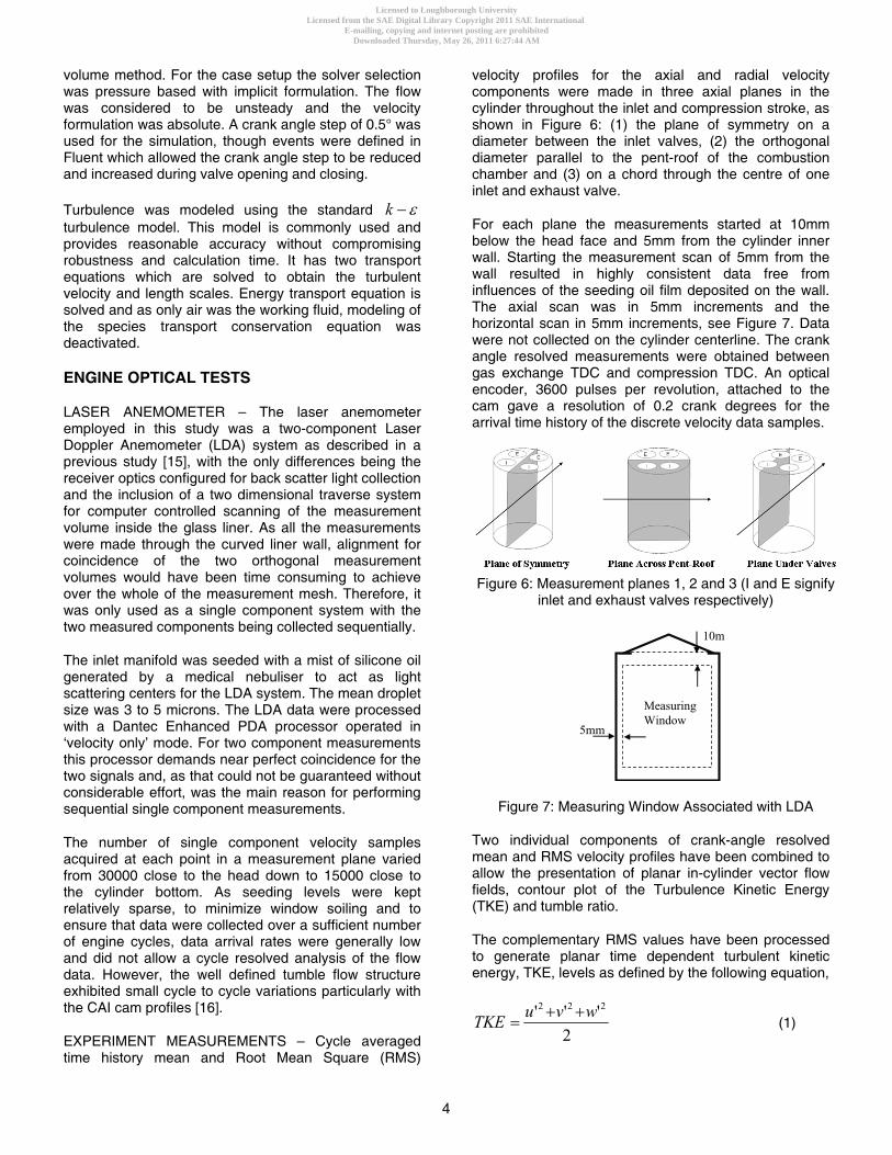
EXPERIMENT MEASUREMENTS – Cycle averaged time history mean and Root Mean Square (RMS)

velocity profiles for the axial and radial velocity components were made in three axial planes in the cylinder throughout the inlet and compression stroke, as shown in Figure 6: (1) the plane of symmetry on a diameter between the inlet valves, (2) the orthogonal diameter parallel to the pent-roof of the combustion chamber and (3) on a chord through the centre of one inlet and exhaust valve.

For each plane the measurements started at 10mm below the head face and 5mm from the cylinder inner wall. Starting the measurement scan of 5mm from the wall resulted in highly consistent data free from influences of the seeding oil film deposited on the wall. The axial scan was in 5mm increments and the horizontal scan in 5mm increments, see Figure 7. Data were not collected on the cylinder centerline. The crank angle resolved measurements were obtained between gas exchange TDC and compression TDC. An optical encoder, 3600 pulses per revolution, attached to the cam gave a resolution of 0.2 crank degrees for the arrival time history of the discrete velocity data samples.

Figure 6: Measurement planes 1, 2 and 3 (I and E signify inlet and exhaust valves respectively)

Measuring Window

5mm

10m

Figure 7: Measuring Window Associated with LDA

Two individual components of crank-angle resolved mean and RMS velocity profiles have been combined to allow the presentation of planar in-cylinder vector flow fields, contour plot of the Turbulence Kinetic Energy (TKE) and tumble ratio.

The complementary RMS values have been processed to generate planar time dependent turbulent kinetic energy, TKE, levels as defined by the following equation,

2''' 222 wvu

TKE (1)

4




where u’, v’ and w’ are the fluctuating velocity components in the orthogonal directions x, y, and z;

As only two components of the RMS velocity were available from the measurements, the third component for this calculation has been taken as the mean of the two measured components.

The mean vorticity for all positions in the plane is used to calculate the tumble ratio of the flow field. For a solid body rotation the vorticity is twice the value of the angular velocity, so, for the tumble ratio calculation the mean vorticity value has been halved [17]. This is given by;

NratioTumble

N

nn

21 (2)

where N is number of vorticity values, and is engine speed in radians/second, and

( )v u

Curlx y

. (3)

For the tumble ratio calculations, a value has been found at the mid point of each set of four vectors on a rectangle in the plane. The tumble ratio is then based on the mean of all vorticity values. By the nature of the point-wise LDA measurements, the curl is calculated in a discrete form.

RESULTS AND DISCUSSION

ENGINE OPERATING CONDITIONS – The initial conditions used to initiate the CFD simulation were obtained from the experimental studies [16] as given in Table 2. The findings from the simulation are presented below.

Table 2: Initial Modeling Conditions

Engine Speed: 1500 RPM

Staring Crank Angle: 360°

Initial Intake Port Pressure: 1 bar

Initial Intake Port Temperature: 298°K

Initial In-Cylinder Pressure: 12 bar

Initial In-Cylinder Temperature: 606°K

Air: Naturally aspirated

Fuel Injection Port Filled

Inlet Valve Opening for HCCI: 423°

Inlet Valve Closing for HCCI: 607°

Maximum Valve Lift for HCCI: 3.6mm

VECTOR FIELDS – Presented in Appendix 2 are snapshots of vector flow fields from CFD simulations and optical engine tests in the plane of symmetry. The left snapshots are experimental results and the right ones are calculated from the CFD calculation. Due to the measuring window associated with the LDA setup see Figure 11, when the processed data is superimposed onto the sketch of the engine geometry to give a visual impression of the flow fields for the experimental study, any flow fields outside this window are not represented. However this does not detract from the discussions between the two studies, as the flow fields and vortices generated in both studies can clearly be observed.

At 422°, the intake valves are closed. The early flow structure being generated within the cylinder is piston dominated and the flow pattern inside the cylinder is uniform with vector arrows pointing down. There is no obvious difference between the experimental and the computational plots.

At 506°, intake valves are opened. The fresh charge from the intake port penetrates into the cylinder. Both the experimental and the computational results showed that the main vortex generated is split into two flows; one is directed straight down the cylinder towards the piston and the other is directed across the cylinder under the exhaust valve.

When the piston further descends at 522°, the in-cylinder flow fields has been further developed, as shown in both measured and calculated results. The lower flow field to the right of the centerline, is counter rotating obstructing the main vortex, thus directing the flow field straight down towards the piston. Observations from both studies show the same flow patterns, expect for the fact that the second developed flow field (the second developed flow field, is due to the splitting of the main vortex generated into two flows and when both flows are redirected by the piston they counter rotate causing the second flow field) in the computational plot appears to be stronger. This is due to the window frame associated with LDA measurement setup, where the experimental plot cannot show this flow field fully, see Figure 7. However from the experimental plot at 522°, if the flow near the piston is projected across onto the computational plot, the flow characteristics compare very well, indicating that if data for this range was available then the flow field could be captured.

As the inlet valve begins to close at 542°, the velocity of the flow fields reduces. Both flow fields exist, the second vortex to the right of the centerline near the piston is still counter rotating, which in turn is limiting the penetration of the main vortex.

5




When the piston moves up the cylinder to 566°, the flow fields in the experimental plot has nearly decayed. The velocity of the vortices on the right hand side of the centerline has also decreased, and with the valve closed the main vortex which existed in this region no longer exists, however the flow directed to the left side of the centre line is still strong in velocity. Both flow fields observed in the previous plot does not exists in the experimental plot, whilst they are still visible in the computational plot, the reason for the lack of representation could be due to the resolution, where the velocities in the experimental are too small to be picked up using the LDA system. The flow fields in both plots are being dominated by the piston.

From close inspection when the structure of the flow fields in both plots at 566° are compared similarities can be drawn. One such similarity are the flows both side of the centerline, which were developed from the main vortex flow which was directed straight down on the right hand side and across the cylinder to the left side under the exhaust valves. The flow directed straight down the cylinder appears in both plots to be directing the flow into the middle of the cylinder, on the other side (flow directed across the cylinder under exhaust valve), the flow is still rotating. The other similarity from observation is the flow in the middle of the cylinder around the centerline were vortex are present. This is more apparent on the computational plots due to the contribution from the piston, but less so on the experimental study as they generated images and are snapshots of the planar flow fields and not based on the full time history of the flow fields. At 662° the flow fields in the experimental study have totally decayed, whilst the computational plots is nearly decayed. The flow fields in both plots are still piston dominated flow filed, as the flow is directed upwards, with very slight circulation.

To summarize, the flow observed in both experimental and computational studies showed two vortices being formed, one just of the centerline at the top to the left and the other to the right of the centerline close to the piston. The two vortices created prevents the penetration of the fresh charge trying to enter the cylinder, this has the adverse effect of directing the flow down the sides of the cylinder, thus limiting the mixing of the fresh charge and the retained residual gases, which in turn will affect the mixture homogeneity at the end of the compression stroke. The flow fields was found to decay as the piston passes through BDC and into the compression stroke. The air motion during the intake stroke is found from both studies to be dominated by the main vortex when the intake valves are opened allowing the fresh charge to flow in, however as the compression stroke commences the air motion is found to be dominated by the piston, especially getting close to TDC. This high degree of correlation between the two studies, can only indicate that through the generation of the geometry and mesh, the fine details/parameters of the real engine has been maintained, as the flow fields

from the computational study reflect those of the experiment.

TUMBLE RATIO – The tumble ratio gives a global number against crank-angle as an indication of bulk flow motion. The vector flow fields in Appendix 2 shows a high degree of correlation between the two studies, but are only snapshots of the planar flow field. The tumble ratio has been calculated to illustrate the global bulk flow against crank angle. It provides a direct comparison of the integral differences between the experimental and computational flow fields. Figure 8 shows the tumble ratios in the symmetry plane obtained from the two studies along with the valve timing.

It can be seen that the measured and calculated tumble ratios curves are overlapped until just before the inlet valve is opening (423°). When the intake valves open, both curves in this zones deviates, with the experimental curve moving into the positive region, whilst the computational curve moves in the opposite direction. This sudden movement from the computational curve into the positive tumble region indicates that the flow momentary becomes reversed. The main reason for this is reverse flow is due to the pressure gradient that exits as a result of the valve opening, as the flow settles with further opening of the inlet valve.

Figure 8: Tumble Ratio for the Symmetry Plan

The reversed flow phenomenon has an adverse effect on the flow, as the production of tumble is slowed when compared to that of the experimental curve. By observing the two curves it can bee seen that the two curves from both studies resemble each other, with the only exception being the timing the tumble is being developed in the computational study. The highest attainable magnitude of tumble for the experimental curve occurs at maximum valve lift, for the computational curve this occurs just before maximum valve lift. The plausible reason for the difference in timing of the highest attainable magnitude of tumble can again be put down to the flow of the computation curve being reversed when the inlet valve was opened, however this should not be considered to be the only reason as a number of parameters can have an effect,

6




such as modelling initial conditions and not being able to replicate the experimental setup to a fine detail.

As the curves move past the maximum valve lift, both curves settle down and begin to ascend into positive tumble. As the inlet valve closes the experimental curve peaks in tumble magnitude as a reaction to the closing of the valves. Towards the end of the compression stroke both curves remain in positive tumble and begin to settle to zero tumble at 720° crank angle. Again just like the vector flow field plots a high degree of correlation between the two studies has been demonstrated to exit, as the bulk flow of the mixture reflect each other.

LOCAL VELOCITIES – The tumble ratio gives a global number for the flow, however it is important to access how the flow behaves from the experimental study to the computational study on a local level. To achieve this, the resultant velocity vector was obtained from the local velocities which was then calculated and plotted, as shown in Appendix 3.

Appendix 3 shows the resultant velocity vector 40mm down from the cylinder head and at specified distance from the cylinder wall in the symmetry plane. The graphs shown in Appendix 3 have been obtained by monitoring 7 different points across the cylinder. In order to understand Appendix 3, a diagram of the monitoring points has been provided, the blue horizontal solid line indicates the distance down from the head (40mm) and the green vertical solid line indicates the distance from the wall (this goes up increments of 5mm from the cylinder wall). Each of the graphs presented have position numbers which can be used on the diagram to located the monitored point. Each point was monitored over the induction and compression strokes.

The graphs from Appendix 3, show that as the monitoring points are moved away from the cylinder wall the accuracy of the velocity magnitude between the experimental and computational study increases. Monitoring points 2 and 4 shows the magnitude difference between the two studies to be high, this difference improves slightly at monitoring point 6, the pattern of improvement can also be observed in monitoring points 8, 10 and 12, but again as the monitoring point gets close to the cylinder the accuracy is once gain lost.

CONCLUSION

An examination of the in-cylinder flow fields on a real engine geometry has been carried out using a commercial CFD package. The results obtained from the CFD study have been validated against experimental results to access whether the generated geometry/computational mesh can be used as a powerful tool to investigate the gas mixing and exchange

processes between the fresh charge (air/fuel) and the trapped EGR within the cylinder of a CAI engine.

The following conclusions are made:

The vector flow field plots indicated that when the intake port is opened, the fresh charge in the intake port flows into the cylinder. Upon entering the cylinder the charge splits into two flows, one directed towards the exhaust valve and the other directly straight down to the piston head. As a result of this action two vortices are generated which limits the penetration of the fresh charge trying to enter the cylinder, thus limiting the mixing of the fresh charge and the retained residual gases, which in turn will affect the mixture homogeneity at the end of the compression stroke.

Assessment of the tumble ratio shown that when the inlet valve opens the momentarily becomes reversed, with the highest magnitude of tumble seen during the valve opening. The reversed flow is more apparent from the computational plot. The cause of this phenomena is thought to be due to the late opening of the valve deep into the induction stroke. This reversed flow was found to retard the flow development, and hence the mixing of the charge and residuals.

Comparisons of measured and predicted local flow velocities show reasonable agreement around the centre of the cylinder.

It can there be concluded that a powerful tool has been generated which can be used to investigate the mixing process in a CAI engine. This high degree of correlation between the two studies, can only indicate that through the generation of the geometry and mesh, the fine details/parameters of the real engine has been maintained, which can accurately predict the in-cylinder process.

REFERENCES

1. Fiveland, S.B. and Assanis, D.N., "A Four-Stroke Homogeneous Charge Compression Ignition Engine Simulation for Combustion and Performance Studies". Society of Automotive Engineers. SAE 2000-01-0332. 2000. pp 1-17

2. Christensen, M., Johansson, B., Amneus, P. and Mauss, F., "Supercharged Homogeneous Charge Compression Ignition". Society of Automotive Engineers. SAE 980787. 1998. pp 1-16

3. Najt, P.M. and Foster, D.E., "Compression-Ignited Homogeneous Charge Combustion". Society of Automotive Engineers. SAE 830264. 1983. pp 1.964-1.979

7




4. Onishi, S., Jo, S.H., Shoda, K., Jo, P.D. and Kato, S., "Active Thermo-Atmosphere Combustion (ATAC) - A New Combustion Process for Internal Combustion Engines". Society of Automotive Engineers. SAE 790501. 1979. pp 1851-1860

5. Ryan III, T.W. and Callahan, T.J., "Homogeneous Charge Compression Ignition of Diesel Fuel". Society of Automotive Engineers. SAE 961160. 1996. pp 157-166

6. Thring, R.H., "Homogeneous-Charge Compression-Ignition (HCCI) Engines". Society of Automotive Engineers. SAE 892068. 1989. pp 1-9

7. Milovanovic, N. and Chen, R., "A Review of Experimental and Simulation Studies on Controlled Auto-Ignition Combustion". Society of Automotive Engineers. SAE 2001-01-1890. 2001. pp 1-10

8. Law, D., Allen, J. and Chen, R., "On the Mechanism of Controlled Auto Ignition". Society of Automotive Engineers. SAE 2002-01-0421. 2002. pp 1-9

9. Christensen, M., Johansson, B. and Hultqvist, A., "The Effect of Piston Topland Geometry on Emissions of Unburned Hydrocarbons from a Homogeneous Charge Compression Ignition (HCCI) Engine". Society of Automotive Engineers. SAE 2001-01-1893. 2001. pp 1-12

10. Aceves, S.M., Flowers, D.L., Martinez-Frias, J., Smith, J.R., Dibble, R., Au, M. and Girard, J., "HCCI Combustion: Analysis and Experiments". Society of Automotive Engineers. SAE 2001-01-2077. 2001. pp 1-7

11. Christensen, M., Johansson, B. and Hultqvist, A., "The Effect of Combustion Chamber Geometry on HCCI

Operation". Society of Automotive Engineers. SAE 2002-01-0425. 2002. pp 1-10

12. Kong, S.C., Patel, A., Yin, Q., Klingbeil, A. and Reitz, R.D., "Numerical Modeling of Diesel Engine Combustion and Emissions Under HCCI-Like Conditions With High EGR Levels". Society of Automotive Engineers. SAE 2003-01-1087. 2003. pp 1-11

13. Kong, S.C., Reitz, R.D., Christensen, M. and Johansson, B., "Modeling the Effects of Geometry Generated Turbulence on HCCI Engine Combustion". Society of Automotive Engineers. SAE 2003-01-1088. 2003. pp 1-11

14. Ansys Fluent, "Fluent 6.3 User's Guide". Fluent Inc. November 2006. pp 1-2226

15. Wigley, G., Hargrave, G.K. and Heath, J., "A High Power, High Resolution LDA/PDA System Applied to Gasoline Direct Injection Sprays". ILASS-Europe, Lisbon. Part. Part. Syst. Charact. 16. 1999. pp 11-19

16. Pitcher, G., Turner, J., Wigley, G. and Chen, R., "A Comparison of the Flow Fields Generated for Spark and Controlled Auto-ignition". Society of Automotive Engineers. SAE 2003-01-1798. 2003. pp 1-8

17. Pitcher, G. and Wigley, G., "LDA Analysis of the Tumble Flow Generated in a Motored 4 Valve Engine". 9th Internal Conference, Laser Anemometry Advances and Applications, Limerick edn.September 2001. pp 1-10

8




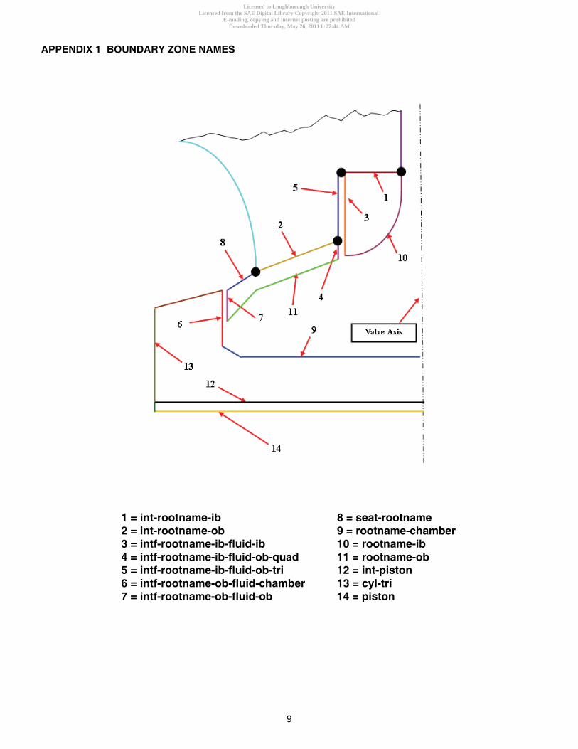
APPENDIX 1 BOUNDARY ZONE NAMES

1 = int-rootname-ib 8 = seat-rootname 2 = int-rootname-ob 9 = rootname-chamber 3 = intf-rootname-ib-fluid-ib 10 = rootname-ib 4 = intf-rootname-ib-fluid-ob-quad 11 = rootname-ob 5 = intf-rootname-ib-fluid-ob-tri 12 = int-piston 6 = intf-rootname-ob-fluid-chamber 13 = cyl-tri 7 = intf-rootname-ob-fluid-ob 14 = piston

9




APPENDIX 2 VECTOR FLOW FIELDS IN THE SYMMETRY PLANE

EXPERIMENTAL COMPUTATIONAL EXPERIMENTAL COMPUTATIONAL

422° 542°

506° 566°

522° 662°

10




APPENDIX 3 Resultant Velocity Vector In the Symmetry Plane

2

-5

0

5

10

15

20

25

350 450 550 650 750

Crank Angle / [Degrees]

Vel

oci

ty /

[m/s

]

ExperimentalComputational

4 6 8

-5

0

5

10

15

20

25

350 450 550 650 750


Vel

oci

ty /

[m/s

]


-5

0

5

10

15

20

25

350 450 550 650 750


Vel

oci

ty /

[m/s

]


-2

0

2

4

6

8

10

12

14

350 450 550 650 750


Vel

oci

ty /

[m/s

]


10 12 14

-5

0

5

10

15

20

25

350 450 550 650 750


Vel

oci

ty /

[m/s

]


-5

0

5

10

15

20

25

30

350 450 550 650 750


Vel

oci

ty /

[m/s

]


-5

0

5

10

15

20

25

30

35

350 450 550 650 750


Vel

oci

ty /

[m/s

]ExperimentalComputational

11




Documents

A CFD model with optical validation on in-cylinder charge ... · validation on in-cylinder charge performances of CAI ... A CFD Model with Optical Validation on In-cylinder Charge