A Case Study on Analytical Analysis of the Inverted

Carnegie Mellon Software Engineering Institute

A Case Study on Analytical Analysis of the Inverted Pendulum Real-Time Control System

Danbing Seto Lui Sha

November 1999

TECHNICAL REPORT CMU/SEI-99-TR-023

ESC-TR-99-023

DISTRIBUTION STATEMENT A Approved for Public Release

Distribution Unlimited

20000204 133

CarnegieMellon Software Engineering Institute Pittsburgh, PA 15213-3890

A Case Study on Analytical Analysis of the Inverted Pendulum Real-Time Control System CMU/SEI-99-TR-023 ESC-TR-99-023

Danbing Seto Lui Sha

October 1999

Dependable System Upgrade

Unlimited distribution subject to the copyright.

PUG QÜALJ3T DKTiJo-i-iid) 1

This report was prepared for the

SEI Joint Program Office HQ ESC/DIB 5 Eglin Street HanscomAFB, MA 01731-2116

The ideas and findings in this report should not be construed as an official DoD position. It is published in the interest of scientific and technical information exchange.

FOR THE COMMANDER

Norton L. Compton, Lt Col., USAF SEI Joint Program Office

This work is sponsored by the U.S. Department of Defense. The Software Engineering Institute is a federally funded research and development center sponsored by the U.S. Department of Defense.

Copyright 1999 by Carnegie Mellon University.

NO WARRANTY

THIS CARNEGIE MELLON UNIVERSITY AND SOFTWARE ENGINEERING INSTITUTE MATERIAL IS FURNISHED ON AN "AS-IS" BASIS. CARNEGIE MELLON UNIVERSITY MAKES NO WARRANTIES OF ANY KIND, EITHER EXPRESSED OR IMPLIED, AS TO ANY MATTER INCLUDING, BUT NOT LIMITED TO, WARRANTY OF FITNESS FOR PURPOSE OR MERCHANTABILITY, EXCLUSIVITY, OR RESULTS OBTAINED FROM USE OF THE MATERIAL. CARNEGIE MELLON UNIVERSITY DOES NOT MAKE ANY WARRANTY OF ANY KIND WITH RESPECT TO FREEDOM FROM PATENT, TRADEMARK, OR COPYRIGHT INFRINGEMENT.

Use of any trademarks in this report is not intended in any way to infringe on the rights of the trademark holder.

Internal use. Permission to reproduce this document and to prepare derivative works from this document for internal use is granted, provided the copyright and "No Warranty" statements are included with all reproductions and derivative works.

External use. Requests for permission to reproduce this document or prepare derivative works of this document for external and commercial use should be addressed to the SEI Licensing Agent.

This work was created in the performance of Federal Government Contract Number F19628-95-C-0003 with Carnegie Mellon University for the operation of the Software Engineering Institute, a federally funded research and development center. The Government of the United States has a royalty-free government-purpose license to use, duplicate, or disclose the work, in whole or in part and in any manner, and to have or permit others to do so, for government purposes pursuant to the copyright license under the clause at 52.227-7013.

For information about purchasing paper copies of SEI reports, please visit the publications portion of our Web site (http://www.sei.cmu.edu/publications/pubweb.html).

Table of Contents

Abstract vn

1 Introduction 1

2 An Analytic Model of Inverted Pendulum System 3

3 Feedback Control Design and Implementation 7 3.1 Controller Design and System Performance 8 3.2 Stability Regions 11 3.3 Controller Implementation 16

4 Design of Control Switching Logic 21 4.1 Safety Region and Safety of the Physical

System 21 4.2 Design of Control Switching Logic 23

5 Conclusions 29

References 33

Appendix A 35 Al Performance Evaluation 35 A2 Stability Region of Linear Control Systems

with Linear Constraints 37 A3 Digitized Control Implementation 40 A4 Delay Caused by Digital Filter 40

CMU/SEI-99-TR-023

CMU/SEI-99-TR-023

List of Figures

Figure 1: An Inverted Pendulum Control System 1

Figure 2: A Small Portion of the Pendulum .3

Figure 3: Friction Model for the Cart 5

Figure 4: Simulation Result 10

Figure 5: The Largest Stability Region (with I'M

and K2 projected to X]~x2 phase plan and x3~x4 phase plane) 13

Figure 6: The Largest Stability Region (with K variable, projected on Xi~x2 phase plan and x3~x4 phase plane) 14

Figure 7: Performance Under Three Controllers 15

Figure 8: The Largest Stability Regions (projected to xl~x2 phase plan and x3~x4 phase plane) 15

Figure 9: Measurement Noises of Track Position and Pendulum 17

Figure 10 : Track Position with Raw Measurement, Filtered Data, and Projected Data 19

Figure 11 Simulation Result 22

Figure 12 : Check if the Physical System is Safe, and if it is Ready for Baseline Control 23

Figure 13 : Application Controller State Transition Diagram 24

Figure 14: Active Controller State Transition Diagram 25

Figure 15: Illustration of Tolerating a Fault Caused by a Brute Force Bug 26

Figure 16 : Lyapunov Function Values 27

Figure 17 : Linear Transformations Between the Physical Position of the Variable and the Ticks (cart position: 0.004365 * ticks; angle: 0.0359 * ticks) 30

Figure 18: Measures for the Transient Response of x(t) 36

Figure 19 : (a) Number of Sampling Periods Delayed as a Function of the Signal Frequency

-

(b) Signals Before and After Filtering 42

CMU/SEI-99-TR-023 iii

iv CMU/SEI-99-TR-023

List of Tables

Table 1: Performance Measures of the Closed-Loop System with Vai and Va2 11

Table 2: Summary of the Comparison on Performance and Stability Region of Three Different

Controllers 16

CMU/SEI-99-TR-023

vi CMU/SEI-99-TR-023

Abstract

An inverted pendulum has been used as the controlled device in a prototype real-time control system employing the Simplex™ architecture. In this report, we address the control issues of such a system in an analytic way. In particular, an analytic model of the system is derived; control algorithms are designed for the baseline control, experimental control and safety control based on the concept of analytic redundancy; the safety region is obtained as the stability region of the system under the safety control; and the control switching logic is established to provide fault tolerant functionality. Finally, the results obtained and the lessons learned are

summarized, and future work is discussed.

TM Simplex is a trademark of Carnegie Mellon University.

CMU/SEI-99-TR-023 v"

viü CMU/SEI-99-TR-023

1 Introduction

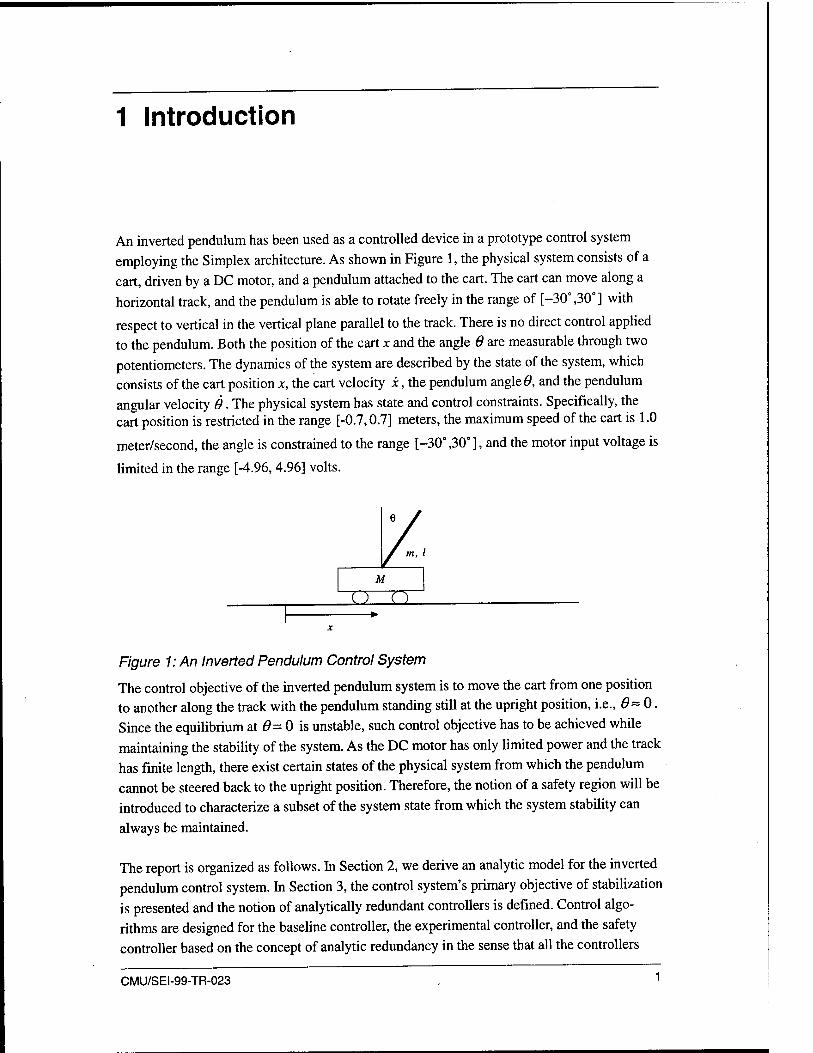
An inverted pendulum has been used as a controlled device in a prototype control system employing the Simplex architecture. As shown in Figure 1, the physical system consists of a cart, driven by a DC motor, and a pendulum attached to the cart. The cart can move along a

horizontal track, and the pendulum is able to rotate freely in the range of [-30° ,30°] with

respect to vertical in the vertical plane parallel to the track. There is no direct control applied to the pendulum. Both the position of the cart x and the angle 6 are measurable through two potentiometers. The dynamics of the system are described by the state of the system, which consists of the cart position x, the cart velocity x, the pendulum angle 8, and the pendulum angular velocity 9. The physical system has state and control constraints. Specifically, the cart position is restricted in the range [-0.7,0.7] meters, the maximum speed of the cart is 1.0

meter/second, the angle is constrained to the range [-30° ,30° ], and the motor input voltage is

limited in the range [-4.96,4.96] volts.

Figure 1: An Inverted Pendulum Control System

The control objective of the inverted pendulum system is to move the cart from one position to another along the track with the pendulum standing still at the upright position, i.e., 6~0. Since the equilibrium at 6= 0 is unstable, such control objective has to be achieved while

maintaining the stability of the system. As the DC motor has only limited power and the track has finite length, there exist certain states of the physical system from which the pendulum cannot be steered back to the upright position. Therefore, the notion of a safety region will be introduced to characterize a subset of the system state from which the system stability can

always be maintained.

The report is organized as follows. In Section 2, we derive an analytic model for the inverted pendulum control system. In Section 3, the control system's primary objective of stabilization is presented and the notion of analytically redundant controllers is defined. Control algorithms are designed for the baseline controller, the experimental controller, and the safety controller based on the concept of analytic redundancy in the sense that all the controllers

CMU/SEI-99-TR-023 1

will achieve the control objective, but they will result in different system performance and stability regions. Practical issues in the implementation of the controllers are discussed. In Section 4, the safety region is defined and the safety criterion of the physical system is described. A control switching logic is established to tolerate the timing and semantic faults. The report is concluded in Section 5 with discussions of the lessons learned and future work on real-time control systems employing the Simplex architecture.

CMU/SEI-99-TR-023

2 An Analytic Model of Inverted Pendulum System

A complete analytic model of the inverted pendulum controlled by a DC motor is derived in three parts, the pendulum-cart dynamics, the friction model, and the motor dynamics. Details

are given below.

Pendulum-cart dynamics: Euler-Lagrange Equation

Let M and m be the masses of the cart and pendulum, / be the length of the pendulum, F be the motor force applied to the cart, and/c mdfp are the friction on the cart and on the pendu-

lum, respectively. The kinetic energy of the cart is Kc = Mx212 and the potential energy of

the cart is zero with respect to a properly chosen reference. For the pendulum, consider a small portion with mass dm located at q e [0,1] as shown in Figure 2.

Figure 2: A Small Portion of the Pendulum

Then we have

\xdm=x+gsine (Xdm=x + qcosee

[ydm=1cose U<*»=-<7sin0ö

kinetic energy of dm:

Kdm=^dm(x2dm+y2

dm) = ±dm(x2+2qcoSexe + q2e2)

and the potential energy of dm:

Pdm=dmgq cos 8

CMU/SEI-99-TR-023

where dm = pdq and p is the mass per unit length of the pendulum. The total kinetic energy

and potential energy of the pendulum can be obtained by integrating Kdm and Pdm from 0 to

/. Doing so, we obtain the total kinetic energy K and the potential energy P of the overall system given by

.. -—(Af + m)x2 + -mlcosdxd + -ml262, P = -. P 2 2 6 2 K = KC+Kp = -(M +m)x2 +-mlcos9x6 + -ml282, P = -mglcos6

and the resulting Lagrangian:

L = K -P = -(M +m)x2 +-mlcos6x6+-ml262 --melcosd 2 2 6 2

Then the Euler-Lagrange equations

dtdx dx /c' dtdO d6~ ip

yield the equations of motion:

(m + M)x +—ml cos 66—mhin662 =F- f 2 2 Jc

—mlcos9x +—ml26 melsm6=-f .2 3 2 '

(1)

p

Friction Model

We assume that both static friction and viscosity friction act on the cart and the pendulum joint. These frictions are described by the following functions:

fc = sgn(x)Axe-c'lil + Bxx, fp = sgn(0) V~C>' + Be6 (2)

with Ax,Bx,Cx,Ae,B0,C0 >0. Friction fc is depicted in Figure 3.

CMU/SEI-99-TR-023

fc

JC<0 -/ '

i>0 Brx

Figure 3: Friction Model for the Cart

Motor Dynamics

The dynamics of the DC motor are governed by the following equations:

Lja =Va-RJa-Eh, Eb=Kbco

Jmd) = Tm-Tl-Bmco

with the relations

where

Tm=KiKTa,Tl=Fr,a>=Kgx/r

La - armature inductance Tm - motor torque (no load)

R - armature resistance Tt - load torque

Ia - armature current

r - driving wheel radius V - armature voltage

CO - motor angular velocity J m - rotor inertia of motor

B„ - viscous friction coefficient

Kj - torque constant

Kb - back-emf constant

Kg - gear ratio

Eb - back emf.

F - force to the cart

Then the motor dynamics can be expressed in terms of Ia, x, and force F as

LJa+RaIa+- K„K s b ;--

^«f-jE+î-î./ =-F

x = Vn

K;K„ (3)

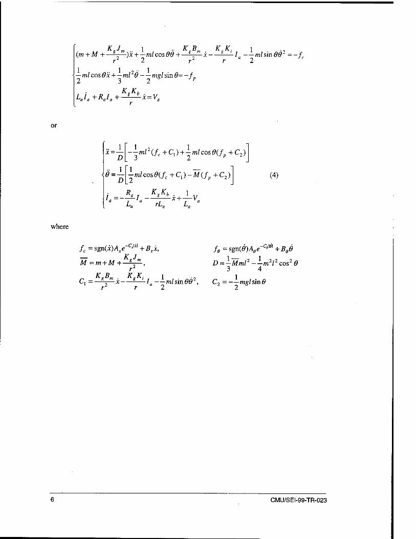
Finally, by combining Eqs (l)-(3), we arrive at a complete model of the inverted pendulum control system with the control variable Va:

CMU/SEI-99-TR-023

K J 1 KB (m + M + -J^) x + - ml cos 66 + —V

r2 2 r2

1 1 ," 1 —mlcos6x +—ml 6—melsmd=-f„ 2 3 2 S Jp

KgKh LJa+RJa+^-^-x = Va

KK S—Ia—mlsin662 = r a 2 ~fc

or

JC = - D

e=— D

—ml2(fc+C}) + -mlcos6(f +C2)

■J-m/cosö(/c+C,)-M(/p+C2) (4)

where

fc=sgn(x)Axe-c>m+Bxx,

M =m + M+—V1, r

c,=- #„£ g m k«"' 1 -/„ mlsin66,

r " 2

csw\ fe=sgn(6)Aee-^m+Bed

D = -Mml2 --m2l2 cos2 6

C2 = —mgl sin 6

CMU/SEI-99-TR-023

3 Feedback Control Design and Implementation

The overall control software consists of three different controllers, Experimental Controller (EC), Baseline Controller (BC), and Safety Controller (SC). A controller is a software mod- ule that implements a control algorithm to compute control commands. Different control algorithms are implemented in EC, BC and SC, and they are designed based on the concept of analytical redundancy. In the Simplex, the active controller is the controller whose control command is actually chosen to be sent to the physical system, and the application controllers refer to the control processes that are replaceable (e.g., the baseline controller and the experimental controller). For a detailed description of the Simplex and its structure in control systems, see Seto [Seto 98]. In this section, we discuss the design and implementation of the

analytically redundant controllers.

Definition 1: Control algorithms are analytically redundant with respect to a requirement R

if they generate control commands satisfying requirement R.

To apply Definition 3.1 to the design of EC, BC and SC, we need first to discuss the requirement that the control algorithms have to satisfy. Apparently, such a requirement is related to the control objective of the system. As we stated in the Introduction, the inverted pendulum is expected to be controlled to move from one track position to another while the pendulum is kept standing still at the upright position. Clearly, it is possible to try to stabilize the system at a new track position from anywhere on the track, but this scheme may lead to a failure of the system, such as the pendulum falling down or the cart running off the track as there are limi- tations on input voltage, track length, and cart velocity. To avoid such failures, we try to stabilize the system at a nearby track position and update the position towards the desired position periodically and at a predefined rate. The desired track position is referred to as a target and the generated nearby track positions are called set points. The set point generation can be done as part of the control algorithm, or be computed separately in a higher level control loop. It is the latter approach that we adopt in this report, which allows separation of con- cerns. In this multi-level control architecture, the lower level control will focus on stabilizing the system at a given set point, while the higher level control takes responsibility for gener- ating proper set points which lead the physical system to the target. Let xs and x, be a set point and a target respectively. Then the control objectives for lower level controllers EC, BC and

SC can be stated as Stabilizing the system in Eq. (4) at [x,x,0,6,Ia] = [>,,0,0,0,0] subject to

the constraints:

CMU/SEI-99-TR-023

x|<0.7, |i|<1.0, |<9|<30°, |Va|<4.96 (5)

and the control objective for the higher level control: Update the set point xs every T seconds with the change vT until the generated set point reaches the target, i.e.,

while (\x, - xt | > |v7|) xs ((k +1)7) = xs (kT) + vT

if (|x,-x,|<|v7|) xs((k + l)T) = x,

Where T is the sampling period of higher level control and v is the desired speed of the cart.

Remark 1: The control objective for higher level control can be considered as a trajectory generation for the cart. Namely, it generates a reference trajectory on track position for the

system to follow. In this report, the reference trajectory is a linear function of time. It is not, however, the only possible reference.

With the control objective defined above, the lower level controllers EC, BC, and SC are said to be analytically redundant, with respect to stabilizing the physical system at a given set point, if all of them will stabilize the physical system at that set point. This definition implies that the control commands generated by EC, BC and SC could be different, but each one of them will stabilize the physical system at the given set point. Because of the constraints on

state and control, the state space of the physical system, [x,x,0,9], is divided to two exclu-

sive regions, feasible region and unfeasible region. The feasible region is defined as a set that contains all the states of the physical system, satisfying all the state constraints. Apparently, any stability region of the physical system has to be a subset of the feasible region. To take into account the constraints, we modify the definition of analytically redundant controllers as: the lower level controllers EC, BC and SC are said analytically redundant with respect to maintaining stability of the physical system in a given region if each one of the controllers will asymptotically stabilize the physical system inside the given region. In this revised definition, we do not require the stability of the system to be guaranteed at a common set point. In fact, we say two controllers are analytically redundant if they both generate control commands within the control limits to asymptotically stabilize the physical system at some set point, which may not be the same, without violating the state constraints. We will require asymptotic stability to guarantee effective control of the cart position. While all the analytically redundant controllers will asymptotically stabilize the physical system, they may result in different system performance and stability region. In the rest of this section, we will investi- gate these differences and propose a design principle for the controllers.

3.1 Controller Design and System Performance It is difficult, if not impossible, to design stabilization control algorithms and identify the corresponding stability regions for the nonlinear system in Eq. (4). Since our interest is to con-

trol the system in a neighborhood of an equilibrium state, it is reasonable to consider the line- arization of the system at the equilibrium. In addition, since the variable Ia is not measurable,

8 CMU/SEI-99-TR-023

and the inductance is relatively small (La = 0.00018 Herry), we reduce the order of the system

by setting La = 0. This leads to

/ = x +—V. rR„ R„

and

x =

6 =

D

_1_ D

■ml2(BlVa-fc-C1) + -mlcose(fp+C2)

-mlcosOiB^ -fc -Cx)-Mtfp + C2)

where

- KB . K2.KtKb „ KgKt B =

~. 1 •+- Q!

r2R„ ».=-2—i,C, = Bx—mlsmdd\C2

rR„ 2 ■ —mgl sin 6

2

Furthermore, we drop the static friction terms by letting Ax = Ae = 0. Then the linearized

system at [xs ,0,0,0] with xs the set point is given by

»22

*42

-a 23

*43

0 fl24

1

-a 44

Xi " 0 "

x3

+ b2

0

_*4. L-*J V = AX+BVn (6)

where

X =[xi,x2,x3,x4]T =[x-xs,x,e,6]T, Dl =4M-3m,

°22=- AB_

D± 65

«42 =' ID

°23=-

a« =■ *43

3mg

A * 6Mg_

ID,

«24=- 6ge

12MB °44=-

0

m/zD,

*,=

K =

4^

6£,

Design of the controllers EC, BC and SC will be based on the linearized model in Eq. (6). In this report, we will concentrate on linear state feedback control in the form Va = KX , al-

though other control synthesis may also be possible, especially for EC. To determine the control gain K, we solve the linear quadratic regulator (LQR) problem: find a control Va such

that the quadratic cost function J(Va) = j^(XTDX + RV2)dt is minimized, where D is a

CMU/SEI-99-TR-023

4x4 symmetric and positive definite matrix and R is positive. The solution to this problem is given by a state feedback control law.

V„ =-R-'B'SX (V)

where S is the solution of the Riccati equation ATS + SA - SBR~lBTS + D - 0. It can be shown that, for each pair of D and R, there exists a unique solution S to the Riccati equation and a control law in Eq. (7) that asymptotically stabilizes the system in Eq. (6) at X = 0.

By varying matrix D and scalar R, the control gain obtained from them can be different, but all the resulting control algorithms will asymptotically stabilize the system at X = 0. The per-

formance of the closed-loop system, however, may not be the same. For the inverted pendu-

lum, we are interested in how good the controller is in terms of controlling the physical sys-

tem to a set point and maintaining its stability there. Such a performance requirement is evaluated by the measures defined in Appendix Al. Namely, we will take a look at the overshoot, settling time and maximum deviation associated with the cart position, the settling time on quadratic state error, and the steady-state value of the accumulated quadratic state error. The following example illustrates the difference in performance caused by different controllers.

5 10 15 Time (seconds)





i2 u-a

#°-4 /*-

o I 2 0.3 I 3 O0.2 i ■^0.1 I E


Solid Lines: results by Vai; Dotted lines: results by Vfl2

Figure 4: Simulation Result

10 CMU/SEI-99-TR-023

Settling time (seconds)

Overshoot (meters)

Maximum derivation (meters)

Settling time on quadratic state error (seconds)

Steady-state value of the accumulated quadratic state error

7.66

0.0

0.36

3.52

0.40

V, al

15.76

0.0

0.36

6.08

0.48

Table 1: Performance Measures of the Closed-Loop System with Va1 and Va2

Example 1: Linearized model of the inverted pendulum control system in Eq. (6), we design the stabilization control laws as in Eq. (7) by choosing two Rs: R = 0.01 and R=0.\, and the same D=diag(l, 1,1,1). We will show that the control laws obtained from these different Rs

will cause different system performance. By running the Matlab, the LQR problem is solved

with the control gains:

£, = [10.0, 27.72,103.36, 23.04] for/? = 0.01

K2 = [3.16,19.85, 69.92,14.38] for/? = 0.1

Suppose the initial condition is chosen as X0 = [0.05,0.31,3.2*^/180,0]. Simulating the

dynamics of the closed-loop system with control Va] = K^Xand Va2= K2X, we obtain the results summarized in Figure 4 and Table 1. From the performance measures, we conclude that the control Val results in a better performance than Va2, while both controllers will stabilize

the system at the equilibrium as indicated in Figure 4.

3.2 Stability Regions While all the analytically redundant controllers stabilize the physical system at X = 0, they may result in different stability regions in addition to different system performance. It can be shown that the closed-loop system performance and the stability region are negatively related, i.e., the better performance of the closed-loop system performance is, the smaller the stability region will be. Generic analysis on such relation will be reported elsewhere, and in this report, we will demonstrate them with the inverted pendulum control system.

We first derive the safety region for a given controller. A stability region of the system in Eq. (6) under the control defined in Eq. (7) is a region in the state space of the physical system, from which the controller is able to asymptotically stabilize the physical system at X = 0 without violating any state or control constraints. We will focus on the stability regions described by a class of quadratic Lyapunov functions. Consider the constraints given by (5) in

X-coordinate:

•0.7-^<^<0.7-^, k <1.0, |JC3|<30, \KX\<4.96

CMU/SEI-99-TR-023 11

Obviously, the constraint on the cart position described above will be as the set point varies. Since the stability region is defined with respect to the equilibrium at a set point and is computed off-line, we would like the constraint on the cart position to be set with respective to the moving set point, i.e., xx =x-xs to be a constant. Since the total track range is [-0.7,

0.7], and the eligible set point range is [-0.5, 0.5], we restrict the cart motion in the range of [-0.2, 0.2] from any given set point, i.e., \xx\ < 0.2 . For the angle constraint, the current speci-

fication is too large, given that all the nonlinearities have been ignored in the linearized model. Hence we reduce the angle range by half. Then a revised feasible region T of the physical system is described by

T = {x\ l^l<0.2, l;c2l<1.0, lx31< 15°, I AX l< 4.96}

and a stability region S of the system in Eq. (7) with a given controller Va = KX is:

s={x\xTPX<l, P>0, ATP+PA<o\ Q r

Apparently, such a defined stability region is not unique for any given controller. To make a comparison on the stability regions between controllers, we consider the largest stability region as defined in Appendix A2. In particular, we first derive the largest stability region for a given controller, and then search the control gain K such that the resulting closed-loop system will have the largest stability region. The former is the case when K is known and the latter corresponds the case that K is known, which are both discussed in Appendix A2.

Case 1. K is given

In this case, our objective is to identify the largest stability region inside the feasible region T for a given controller. The control gain has been obtained with other consideration, for instance, they could be chosen to satisfy some particular performance specifications. To find the largest stability region, we follow the procedure described in Appendix A2 and formulate the following LMI problem to determine matrix Q = P_1:

minimize log det Q _1

subject to QAT +AQ<0, Q>0

a\Qak<\, k = l,...,S,

where

a, =[5,0,0, Of, fl3= [0,1,0, Of, a5= [0,0,3.82, Of, a7=K/4.95,

a2= [-5,0,0,Of, a4=[0,-l,0,0f, a6=[0,0,-3.82,Of, as=-K/4.95.

This LMI problem is solved by the algorithm developed in Vandenberghe [Vandenberghe 98], and the resulting stability region, projected to xx~x2 phase plan with x3 = xA = 0 and x3~x4

phase plane with xx = x2 = 0, are shown in Figure 5.


s 1 £ 0.5

* 0

'I -0.5

x -1

•

I ■

It— ~——^ I > I

I

. -0.2 -0.1 0 0.1 0.2

x1 with K1 (meter)

5 1

E. 0.5 CM * n

§ -0.5 X -1

-0.2 -0.1 0 0.1 0.2 x1 with K2 (meter)

^ 100

50

0

'i -50

x -100

-20 -10 0 10 x3 with K1 (deg)

■S2 co

CM

100

50

i -50 x

-100 -20 -10 0 10

x3 with K2 (deg)

20

20

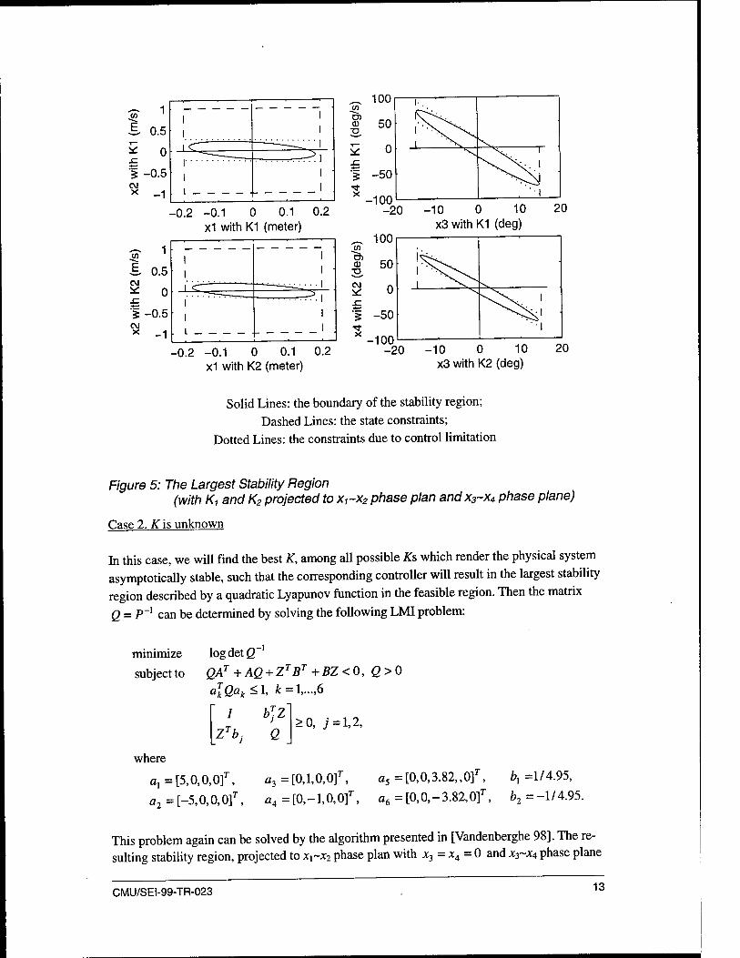
Solid Lines: the boundary of the stability region; Dashed Lines: the state constraints;

Dotted Lines: the constraints due to control limitation

Figure 5: The Largest Stability Region (with Ki and K2 projected to x1~x2 phase plan and x3~x4 phase plane)

Case 2. K is unknown

In this case, we will find the best K, among all possible Ks which render the physical system asymptotically stable, such that the corresponding controller will result in the largest stability region described by a quadratic Lyapunov function in the feasible region. Then the matrix

Q = P~l can be determined by solving the following LMI problem:

minimize log det Q~

subject to QAT + AQ + ZTBT + BZ < 0, Q > 0 o[Qak < 1, k = 1.....6

b)Z

Z'bj Q >0, ;=1,2,

where

ax = [5,0,0,0f, a, = [0,l,0,0f, a5 = [0,0,3.82,, Of, \ =1/4.95,

a2 = [-5,0,0,0f, a, =[0,-1,0, Of, a, =[0,0, -3.82, Of, b2 =-1/4.95.

This problem again can be solved by the algorithm presented in [Vandenberghe 98]. The resulting stability region, projected to x^~x2 phase plan with x3 = x4 = 0 and *3~JC4 phase plane


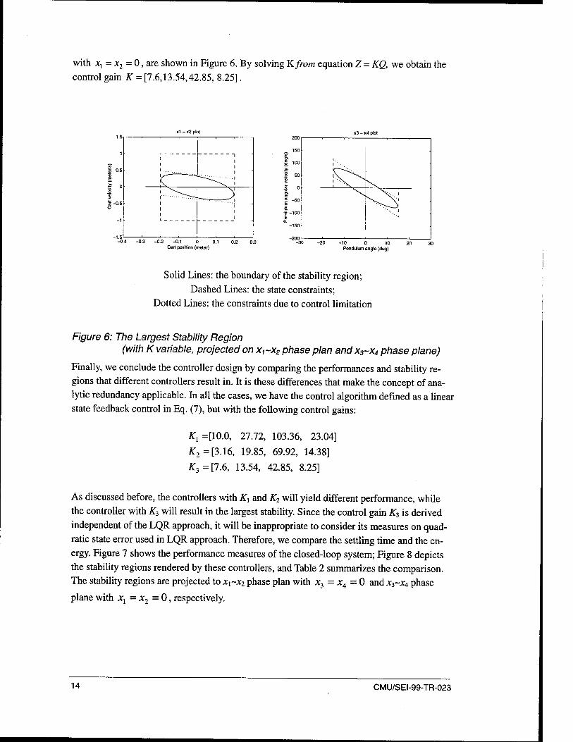
with xx = x2 = 0, are shown in Figure 6. By solving Kfrom equation Z = KQ, we obtain the control gain K = [7.6,13.54,42.85, 8.25].

x1 - x2 plot x3 - x4 plot

| «4 i

0.4 -0.3 -0.2 -0.1 0 0.1 0.2 0.3 Cart position (meter)

-10 0 Pendulum angle (deg)

Solid Lines: the boundary of the stability region; Dashed Lines: the state constraints;

Dotted Lines: the constraints due to control limitation

Figure 6: The Largest Stability Region (with K variable, projected on x,~x2 phase plan andx3~x4 phase plane)

Finally, we conclude the controller design by comparing the performances and stability regions that different controllers result in. It is these differences that make the concept of analytic redundancy applicable. In all the cases, we have the control algorithm defined as a linear state feedback control in Eq. (7), but with the following control gains:

ATi =[10.0, 27.72, 103.36, 23.04]

#2 =[3.16, 19.85, 69.92, 14.38]

£3 =[7.6, 13.54, 42.85, 8.25]

As discussed before, the controllers with Kx and K2 will yield different performance, while the controller with K3 will result in the largest stability. Since the control gain K3 is derived independent of the LQR approach, it will be inappropriate to consider its measures on quadratic state error used in LQR approach. Therefore, we compare the settling time and the energy. Figure 7 shows the performance measures of the closed-loop system; Figure 8 depicts the stability regions rendered by these controllers, and Table 2 summarizes the comparison. The stability regions are projected to xx~x2 phase plan with x3 = x4 = 0 and x3~x4 phase

plane with x\ - x2 = 0, respectively.



20 0.62

2 4 6 8 10 Time (seconds)

Dashed Lines: results corresponding to control K]X; Dotted Lines: obtained with K2X;

Solid Lines: generated by K3X

Figure 7: Performance Under Three Controllers

x1 - x2 plot x3 - x4 plot

-0.8 -0. 2 -0.1 0 0.1 0.2

Cart position (meter)

100

80

"§> 60 o ■D ^ 40 .*; o % 20 > fe 0 3 D) i -20 E .2 -40

-60

-80

-100

V "" ~~ ' -^^s.

\ "V -v '. \

\ "N ^ '■■ \ *•> V

/ ■'"

/

>v '■ .X

- v. V . \ ■. 'v X- \

-15 -10 -5 0 5 Pendulum angle (deg)

10 15

Dashed Lines: the results corresponding to control KXX

Dotted lines: obtained with K2X

Solid lines: generated by K3X

Figure 8: The Largest Stability Regions (projected to x1~x2 phase plan andx3~x4 phase plane)


KXX K2X K,X

Settling time (seconds) 7.66 15.76 8.44 Overshoot (meters) 0.0 0.0 -0.152 Maximum derivation (meters) 0.36 0.36 0.37 Settling time on energy (seconds) 2.92 2.86 4.64

Measure of the size of stability region, (^/det Q ) 0.0078 0.0144 0.0279

Table 2: Summary of the Comparison on Performance and Stability Region of Three Different Controllers

The above comparison shows that the controller with K3 does give the largest stability region,

but has the worst performance among all three controllers. On the other hand, the controller with gain K^ yields a smallest safety region but has a much better performance. All three controllers are analytically redundant with respect to stabilizing the inverted pendulum at the equilibrium X = 0. Then the principle of controller design can be stated as: the control gain associated with a larger stability region should be used to construct a safety controller, while the control gain corresponding to better performance ought to be adopted for the baseline controller and the experimental controller.

3.3 Controller Implementation In the inverted pendulum control system, the control algorithm for all the analytically redundant controllers are the same, namely, linear state feedback control u = KX but with different control gains. These control gains are determined from solving LQR problems with the objective that the system performance under the baseline controller and the experimental controller will be satisfactory with respect to some performance specification, while the safety controller will offer the largest stability region among all these controllers. It is worth noting that the model that we use to compute the control gains is only an approximation of the real system, in which we have ignored all the nonlinearities, static frictions, motor dynamics, and other the uncertainties on dynamics and parameters. Therefore, the resulting control gains are expected to be off from the gains that should be actually used, and it is important to adjust them in experiments. Let Kb, Ke and Ks be the control gains for the base-

line controller, the experimental controller and the safety controller, respectively. The following gains have been used for one inverted pendulum control system

Kb = [10.0, 36.0, 140.0, 14]; Ke= [8.0, 32.0, 120, 12]; K,= [6.0, 20.0, 60.0, 16.0]

These controllers are implemented with a sampling frequency 50 Hertz.

In addition to model imprecision, the measurements of the track position and the pendulum angle are noisy are well. Since these are the only states can be measured from the physical system, the cart velocity and the pendulum angular velocity have to be constructed separately. Therefore, how to filter the measured data and construct the unknown states affect directly


the precision of the states that are used to compute the control command. From Figure 9, it is clear that the measurement noises1 are above 5HZ. Hence a first-order digital Butterworth lowpass filter with cut-off frequency 5HZ is used. To construct the velocities, we apply the

first order approximation, namely

x(t) = [x{t)-x{t-T)VT and e(t) = [e(t)-6(t-T)]/T

with T the sampling period. Although the position data in above construction are the results after filtering, they may still contain certain amount of noise. When the remaining noises are still relatively large, we extend the first order approximation over more periods to raise the

signal-to-noise ratio. In those cases, we would have

x(t) = [x(t)-x(t-mT)]/mT and 0{t) = {6{i) - d{t - mT)V mT

where m is an integer greater that one. Our experiments showed that, with m = 2, the constructed velocities are much more clean than the case when m = 1, but they suffer further delay. Therefore, the trade-off between clean velocity and the delay need to be carefully considered. For alternatives of velocity construction, one may consider using Kaiman filter which eliminates the delay in data filtering and generates accurate velocity estimates simultane-

ously.

Measurement Noise on Track Position K j 0-3 Measurement Noise on Pendulum Angle

Frequency

Figure 9: Measurement Noises of Track Position and Pendulum

Another practical issue in control implementation is delay. As we discussed in Appendix A4, a digital filter will cause delay. In fact, the lowpass digital filter that we used will cause 1-2 sampling periods delay. We will call such delay as filtering delay. While the effect of these delays can be compensated by adjusting the control gains in the control law, such delay will have a significant effect on safety checking of the system, as described in a later section. In addition to the filtering delay, the control implementation also causes one period delay. Spe-

1 The noises shown are the difference between the physical measurements and the clean data. The clean data is obtained by filtering the raw data forwards and backwards using a high order lowpass filter, e.g., 10th order. While such filtering gives noiseless data with no delay, it can only be done off- line.


cifically, at each sample, the measured data is acquired and the computed control command is sent out. During one sampling period, for example, in (t0, tQ+T), the control command

u(t0 +T) is computed based on the state sampled at time tQ, x(t0). This control will not be

sent out to the physical system until the end of the period, i.e., t0+T .

At time t0 + T, however, the state of the system has been evolved to x(t0 + T). Therefore,

the control command will always act on the state that is one period later than the state from which the command was computed. We refer such type of delay as digital implementation delay. One may argue that the control command should be sent out right after it is computed, given that the computation of control command could be very short. While this arrangement

can reduce the implementation delay, it may cause jittering and makes the scheduling of control tasks difficult if there are multiple tasks executing in a uniprocessor. We intentionally

choose the implementation with one period delay to avoid jittering and to ease the schedula- bility analysis.

Both the filter delay and the digital implementation delay can be compensated by the model- based state projection, i.e., projecting state by solving the system equations. See Appendix A3

for detailed computation. Let F = eAT,G=i eArdt. Then the compensation of these delays

in period (t0,t0 +7)can be described as below.

Filtering delay compensation

Suppose there is one period filtering delay. Upon receiving the measurements from the physical system t0, we feed the data to the lowpass filter. Then the filtered data can be considered

as the true (noiseless) track position and pendulum angle at the previous sample, i.e., [x(t0 -T), 0(tQ -T)] . Constructing the velocities based on the filtered data, we obtain the

full states at t0 -T , X(t0-T). Since the control command u(t0 -T) was output to the

physical system at t0 -T and it acted on the state X(t0 -T), the full state at time t0 can be

projected as:

X(t0) = FX(t0-T) + Gu(t0-T)

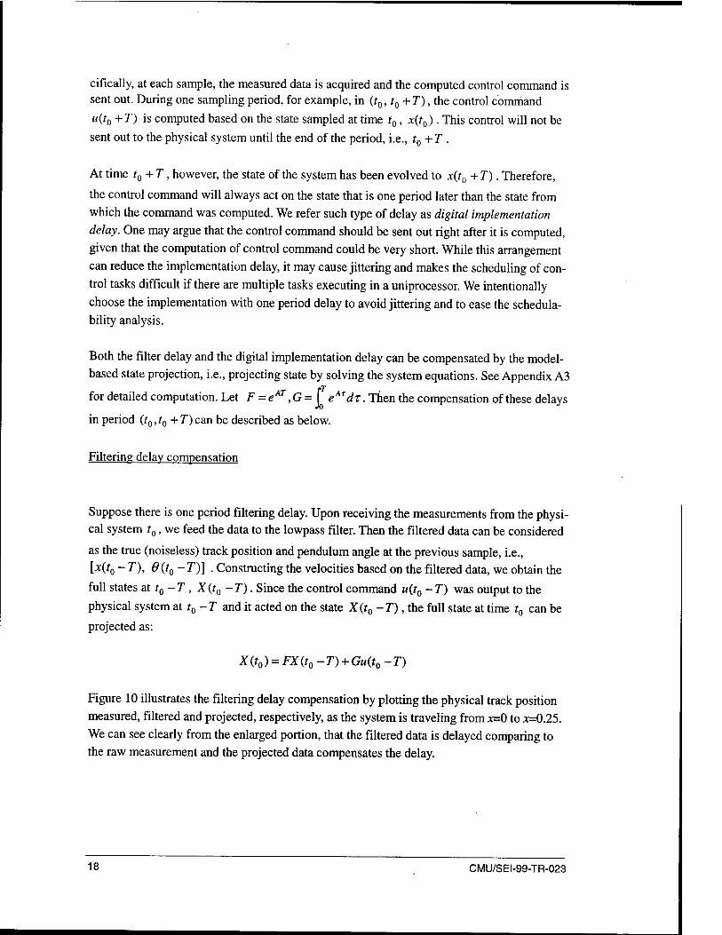
Figure 10 illustrates the filtering delay compensation by plotting the physical track position measured, filtered and projected, respectively, as the system is traveling fromx=0 to JC=0.25.

We can see clearly from the enlarged portion, that the filtered data is delayed comparing to the raw measurement and the projected data compensates the delay.


0.07

5 10 15 20 Time (seconds)

25 0.01

3.9 4 4.1 4.2 4.3 4.4 Time (seconds)

Solid Lines: plot of the track position with the raw measurement Dashed Lines: the filtered data

Dotted Lines: the projected data

Figure 10: Track Position with Raw Measurement, Filtered Data, and Projected Data

Digital implementation delay compensation

The control command u(t0) has been sent out to the physical system at time t0. The noise-

less state of the physical system at t0 is obtained from the compensation of the filtering de-

lay. Then to find out at what state that the control command u(t0 + T) will start influencing

the physical system, namely, what state that the physical system will be at the time t0 + T

under the control u(t0), we project from X(t0) for one more period:

X(t0+T) = FX(t0) + Gu(t0)

This is the state at which the physical system will response to the control command u(t0 + T). Then we compute u(t0 + T) from the projected state X (t0 + T). While the digital

implementation delay can be dealt with by model-based state projection, it is actually compensated for by adjusting the control gains properly in the experiments because the state feedback control is reasonably robust with respect to small delay. State projection will com-

pensate for it in state safety checking discussed later.



4 Design of Control Switching Logic

The control switching logic in the Simplex is designed to tolerate timing faults and semantic faults. It governs the selection of the active controller such that the safety controller will be chosen if a fault is detected, and the baseline controller will be in charge once the system is recovered from a faulty situation. To detect a timing fault, it is simply to check if the application controllers have missed their deadlines. For semantic fault, however, the detection is more involved. In the follows, we will first discuss an abstraction of the continuous dynamics of the physical system for semantic fault detection, and then design the control switching

logic.

4.1 Safety Region and Safety of the Physical System The analytically redundant controllers in the Simplex architecture will result in different stability regions. By evaluating the state of the physical system relative to the stability regions, control switches can be executed to tolerate the semantic faults. In particular, the safety controller is designed to provide safety protection, and therefore, the stability region of the safety controller is of special importance. In this section, we define the notion of the safety region and the safety criterion of the physical system, which will be used for the design of control

switching.

A semantic fault is detected based on the behavior of the physical system. To abstract the continuous dynamics of the system, we define the safety region as the following: The safety region with respect to the safety controller us is defined as the largest stability region of the physical system under the control of us. Let Ps be the positive definite matrix which renders the stability region of the system to the largest. Then the safety region SR is given by SR = {x\XTPsX < l}. A state X0 is inside SR if XQ

TPSX0 < 1. Hence we would like to say

that the physical system is safe if its state is inside the safety region, and for tolerating a semantic fault, we would design a switching logic to invoke the safety controller whenever the state of the physical system is out of the safety region. Such strategy, however, will not work. By the definition of stability region, it is clear that the physical system may not be stabilized if it starts from a state outside the stability region. Thus it would be too late for the safety controller to maintain system stability once the state of the physical system is out of its stability region. We refer this situation as the safety region paradox. To fix this problem, we need to know, at time t0, if the state of the physical system at t0+T will be inside the safety region. If it is not, we would like to switch to the safety controller at tQ. Given the filtering delay and digital implementation delay in the system, such a "look ahead" strategy can be extended as the following. Suppose (t0,t0 +T) is the period that the control switching logic


needs to make a decision if the safety controller's output should be used. Let z(t) = [xm(t), 6m(t)] and [x(t), 6 (t)] be the measurements and the noiseless data of the

track position and the pendulum angle, respectively. Figure 11 shows the inputs from and outputs to the physical system.

in: z(t0-T) in: z(t0) in: z(t0+T) ,-„: Z(t0+2T)

out: u{t0- T) out: u(t0) out: u(t0 + T) 0ut: u(t0 + IT)

' 1 ' ♦ ' Ä ' " u(t0) = KX(t0-T) u(t0+T) = KX(t0) u(t0+2T) = KX(t0+T)

Solid Lines: results by Vai; Dotted Lines: results by Va2

Figure 11: Simulation Result

Step 1. Filtering delay compensation

In this first step, the measurements z(t0) is obtained from the physical system. Following the

compensation procedure described in last section, the true state of the physical system at time r0 can be obtained from

X(t0) = FX(t0-T) + Gu(t0-T)

Step 2. Digital implementation delay compensation

Again, as derived in last section, the state from which the physical system will response to the control command u(t0 +T) is given by

X(t0+T) = FX(t0) + Gu(t0)

Step 3. One more period projection to resolve the safety region paradox

If the safety controller were chosen as the active controller in the time interval (t0,t0 +T), it

would affect the physical system at t0 + T . Therefore, the state X(t0 + T) can not be used to

determine if the safety controller should be selected due to the safety region paradox. This implies that one more period state projection is needed. If the further projected state is out of the safety region, the safety controller will be switched to active and starts controlling the physical system at t0 + T , at which the state of the physical system is still inside the safety

region.


For this projection, we use the control command that is going to be sent out to the physical system. Let such control be u(t0 +T). Then the projection from X(t0+T) under u(t0 +T)

is given by

X(t0+2T) = FX(t0+T) + Gu(t0+T)

Then the safety criterion of the physical system is given as: the physical system is safe the

state X(t0 + 27) is inside the safety region, i.e., X(tQ + 2T)T PsX(t0 +2T)<1; otherwise, it

is unsafe. Let Pb > 0 be the matrix that gives the largest stability region of the physical sys-

tem under the baseline control. We say that the physical system is ready for the baseline control if the state X(t0 +T) is inside the stability region given by Pb, i.e.

X(t0 +T)TPhX(t0+T) < 1; otherwise, it is not ready. These are summarized in Figure 12.

Input at t measurement W'o). 0 (to)]

I filtering and velocity construction

I X(t0-T) State projection with previous controlu/t _j\ Physical system is not ready for BC

[ X(t0) No X(t0 +T)

State projection with current control u{tQ) *\X£o+TJ RX(hJrT)^(!s^~*'

,, Xifo+T)

State projection with future control u(t +T)

Physical system is ready forBC.

X(t + 2T) — ►Cx (f0 +27T Ps X(f0 + 2T)< ^V~~^

No UNSAFE - implies a semantic fault

Figure 12: Check if the Physical System is Safe, and if it is Ready for Baseline Control

4.2 Design of Control Switching Logic The control switching logic is designed based on the detection of timing fault and semantic fault. The former is simply to check if the application controllers have missed their deadlines, while the latter is to evaluate the state of the physical system with respect to the safety region. In addition to the behavior of the physical system and the timing performance of the application controllers, the user interface provides a way to manually affect the selection of the active controller by changing the availability of the application controllers. The state of an ap-

plication controller is defined as follows:


Enabled the controller is running and its output can be chosen to be sent to the physical system

Disabled the controller is running but its output is disabled Terminated the controller is destroyed

When a controller is destroyed, all of the resources it has been allocated are released. For the inverted pendulum control system, the following assumptions have been imposed:

• When an application controller changes from being active to inactive because of a fault it contains, its output will be disabled until the user re-enables it.

• If both the experimental controller and the baseline controller are running with valid control commands, the experimental controller will be selected as the active controller.

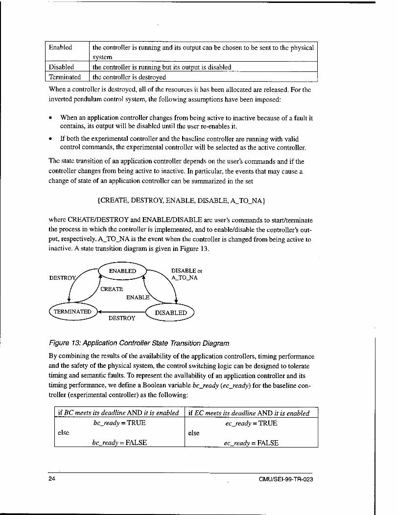
The state transition of an application controller depends on the user's commands and if the controller changes from being active to inactive. In particular, the events that may cause a change of state of an application controller can be summarized in the set

{CREATE, DESTROY, ENABLE, DISABLE, A_TO_NA}

where CREATE/DESTROY and ENABLE/DISABLE are user's commands to start/terminate the process in which the controller is implemented, and to enable/disable the controller's output, respectively. A_TO_NA is the event when the controller is changed from being active to inactive. A state transition diagram is given in Figure 13.

ESTROY/ ~( ENABLED J~ -^ DISABLE or

\A_TO_NA

/ CREATE \

ENABLE^

TERMINATED y* v DESTROY ^>

DISABLED")

Figure 13: Application Controller State Transition Diagram

By combining the results of the availability of the application controllers, timing performance and the safety of the physical system, the control switching logic can be designed to tolerate timing and semantic faults. To represent the availability of an application controller and its timing performance, we define a Boolean variable bcjready (ecjeady) for the baseline controller (experimental controller) as the following:

if BC meets its deadline AND it is enabled if EC meets its deadline AND it is enabled bcjready = TRUE

else

bc_ready = FALSE

ecjready = TRUE else

ecjready = FALSE


Suppose a control command with a value out of the allowable range (command invalid) is considered to be caused by a semantic fault in the controller. To describe the behavior of the physical system with relation to system safety and recovery from a faulty situation, define

Boolean variables safe and to_bc with the following assignments:

if control output is valid AND the physical

system is safe

else

safe = TRUE

safe = FALSE

if previous active controller is SC AND the physi-

cal system is ready for BC

else

to_bc = TRUE

to be = FALSE

Define the state of the active controller to be

{BASELINE, EXPERIMENTAL, SAFETY}

Then the state transition of the active controller will be determined by the values of the Boo- lean variables bc_ready, ec_ready, safe and injbe. Figure 13 shows the state transitions of the active controller when the Boolean expressions on the transition arcs are TRUE.

.'safe or !bc_ready & lecjready.

BASELINE

SAFETY

ecjready 'bejready & lecjready & tojbc

safe & ec_ready

Isafe or 'bejready & lecjready

X bejready & lecjready & safe

ÊXPERIMENTAL,

Figure 14: Active Controller State Transition Diagram

We have now completely established the control switching logic to determine the active controller. Implementation of this logic amounts to coding the state transition diagrams in Fig- ures 13 and 14. To illustrate this control switching logic, we present the following example.

Example 2: Suppose the mission was to move the inverted pendulum from* = -0.4 to x = 0.4. All three controllers were running and the experimental controller initially controlled the system. A brute-force bug2 was coded in the experimental controller and it triggered while the inverted pendulum was moving to the target. Upon detection of the bug, the active controller was switched to the safety control, and remained under safety control until the physical system was ready for the baseline control. Here we have used a reduced size safety region as the

stability region of the baseline controller, namely, the region given by \X \XTPSX < 0.4). To

further reduce the effect of the noise on the value of Lyapunov function, we filtered the computed value of the Lyapunov function with a high order lowpass filter. The result was then

2 An experimental controller with a brute-force generates the control command with the maximum (or minimum) control value allowed every sampling period.


used for the recovery check, a check to see if the physical system would be ready for the baseline control, i.e., if the filtered value is less than the threshold for recovery, 0.4. This delayed the switch to the baseline controller, but it guaranteed that the safety controller would not be switched back after the baseline controller was chosen to be the active controller.3

Figure 15 shows the trajectories of the physical system, and Figure 16 displays the results of safety checking and controller switches. As we can see from the figures, the experimental controller initially controlled the system, and it caused the system to behave badly after 11 seconds. At t = 11.02, the value of the Lyapunov function jumped over 1 and the bug was detected. At the same time, the safety controller was taking over the control. After one period since the safety controller was in charge, the value of the Lyapunov function dropped below

1, but the physical system was not ready for the baseline control yet. Having been controlled

by the safety controller for four periods, the physical system became more stable, and the

value of the Lyapunov function was reduced lower than 0.4. Hence at t = 11.1, the baseline controller was switched active, and remained in control afterwards.

o

O £L X. O co

CO

c < E

T3 C

-0.5

0.05

£ -0.05

5 10 15 Times (seconds)


20



20

Figure 15: Illustration of Tolerating a Fault Caused by a Brute Force Bug

Theoretically, the value of the Lyapunov function should decrease monotonically under the safety controller, but it may not be the case in reality due to the measurement noise, the inaccuracy in system model and the construction of velocities. As a result, the value of the Lyapunov function can drop to a low level after the safety controller takes over control, which may trigger the switch to the baseline controller, and then bounce back to above 1 to knock out the baseline controller again.


M .JN 5 10 15

Times (seconds) 10.7 10.8 10.9 11 11.1 11

Times (seconds) 10.7 10.8 10.9 11 11.1 11.2

Times (seconds)

(a) Value of the Lyapunov Function with Thresh-

old 1

(b) A Blowup Portion of the Value of the Lyapunov

Function 1 Solid Line: unfiltered values, used for safety check

with threshold 1; Dotted Line: plots the fil-

tered value, used for recovery check with threshold

0.4

(c) Safety of the Physical

System Solid Line: the safety of the physical system (1 -

safe and 0 - unsafe); Dotted Line: the state of the active controller (1-

safety controller, 2- baseline controller, and 3 - experimental con-

troller)

Figure 16: Lyapunov Function Values



5 Conclusions

In this report, we described analytical approaches for designing analytically redundant controllers, deriving the safety region, and establishing a control switching logic in an inverted pendulum control system using the Simplex. While these approaches were developed in asso- ciation with a particular control system, the general analytic framework should be applicable

to other control applications without much difficulty.

Analytic redundancy is the key concept in the Simplex architecture. Based on this concept, the baseline controller, the experimental controller, and the safety controller were designed as linear state feedback controls with the common requirement of asymptotically stabilizing the physical system at an given equilibrium state. While all of the controllers will achieve this goal, the closed-loop systems may have different performance in terms of the rate of conver- gence to the equilibrium and different stability regions. With certain well-defined performance measures, it can be shown that the performance of the closed-loop system is negatively related to the size of the corresponding stability region. Namely, the better performance the closed-loop system has, the smaller its stability region will be. It is this property that allows us to design the safety controller to render a large stability region although the performance it yields may not be superior, and the application controllers to focus on improving the performance while the stability regions they result in may be small. Such a combination enables an application controller to explore high functionality under the protection of the safety con-

troller.

The safety region is defined as the largest stability region rendered by the safety controller. It is derived by solving a LMI problem subject to stability requirements as well as the state and control constraints. Two cases were considered: 1) derive the safety region for a given safety controller; and 2) design the safety controller such that the resulting safety region is maxi- mized. In the latter case, the resulting stability region is the largest one described by a quadratic Lyapunov function among all possible linear state feedback controllers that asymptotically stabilize the physical system. For testing in the lab, we used the safety region derived with a given safety controller whose control gains have been adjusted in the real system for

an acceptable performance.

The control switching logic was designed to tolerate the timing and semantic faults. It was established by taking into account the availability of the application controllers, the timing performance of the application controllers, and the safety of the physical system. The key step in the logic design is to correctly represent the state transition of the application controllers and the state transition of the active controller. While the specifications on fault tolerance


may vary from application to application, the basic structure of the state transition diagrams will remain the same, and design procedures can be carried over cross applications.

As the analytic approaches were employed in the real control system, there are practical/engineering issues need to be addressed. Many of them have occurred in our implementation, and we will discuss four of them here. First, the physical system needs to be well calibrated. The measurements of the track position and the pendulum angle are obtained from two potentiometers. After the A/D converter, the signals from the potentiometers are con- verted to digital ticks. Therefore, transformations from the ticks to the physical positions of the variables measured are needed. To derive such transformations, we manually move the cart to different locations on the track and fix the pendulum at different angles, and for each of these positions, record the tick readings. By applying least-square fitting, we found the linear relation between the physical position of the variable measured and the ticks read as in Figure 17.

-0.8 -1500 -1000 -500 0 500 1000 1500

Reading (ticks) - Ticks at Track Center

40

30

20

S 10

-20

-30

-40 -1000 -500 0 500

Reading (ticks) - Ticks at Angle=0 1000

Figure 17: Linear Transformations Between the Physical Position of the Variable and the Ticks (cart position: 0.004365 * ticks; angle: 0.0359 * ticks)

In addition to identifying the transformations, it is important to get the precise tick readings at the track center (x = 0) and zero angle (6 = 0). These two measures may need to be re- calibrated from time to time.

Second, the accuracy of the analytic model is important. As we have seen, both the model- based state projection and the derivation of the safety region are based on the analytic model. While the control algorithm is robust with respect to imprecision in the model, model-based state projection and the derived safety region could suffer significantly because of imprecision in the estimation of the run time system state and the model of the plant. The current model of the inverted pendulum was completely derived from mechanical principles, and some of its parameters were adjusted by comparing the simulation of the model and the results obtained from running the physical system. This guarantees the accuracy of the model in a short term, i.e., the matching results of simulation and the physical system trajectory in a


short time, say a few periods. For state projection in a longer time, we ought to carry through an extensive system identification procedure. This is certainly possible for a system like the inverted pendulum whose linearized model well represents the actual nonlinear system.

Third, the velocity construction plays an important role in both model-based state projection as well as the safety checking. When the state projection did not give a satisfactory result, the reason could be the inaccuracy of the model as we discussed above, but it is also possibly due to the approximation of velocities. As the position variables contain noise, the velocity approximation could be very poor. On the other hand, since the safety evaluation of the physical system dependents on the calculation of a quadratic Lyapunov function, which involves the full states, the result obtained could be off significantly if the velocity components are poorly constructed. To resolve the velocity construction problem, the standard approach is to build an observer, or Kaiman filter if noise is one of the issues need to be dealt with. Again this is a model-based methodology, and therefore, it would be better to be use it in conjunction with a model identification approach, even though Kaiman filter would tolerate a certain inaccuracy of the model. This is one of the subjects for further research.

Finally, in design of the safety controller, one objective is to make the corresponding stability region to be as large as possible, but his should not be pushed too far. As we discussed earlier, the larger the stability region is, the poorer the performance will be in the closed-loop system. In the inverted pendulum system, if the control gain is chosen such that the safety region is too large, the corresponding safety controller would take a longer time to drive the physical system to a neighborhood of the equilibrium state after it takes over the control from a faulty controller. Therefore, in the actual design, we need to make a trade-off between the volume

gained and performance lost.

While the inverted pendulum is a prototype system, it certainly contains a lot of control issues. We would like to emphasize that the analytic approaches developed to address these issues can be very well extended to other control applications, including large-scale control systems. On the other hand, of course, there are still some unsolved problems and they will

be investigated in our future research.



References

[Boyd 94] Boyd, S.; El Ghaoui, L.; Feron, E.; & Balakrishnan, V. "Linear Matrix Inequalities in System and Control Theory." SIAM Studies in

Applied Mathematics. Philadelphia, PA: Society for Industrial and

Applied Mathematics (SIAM), 1994.

[Vandenberghe 98] Vandenberghe, L.; Boyd, S.; & Wu, S.P. "Determinant Maximiza- tion with Linear Matrix Inequality Constraints." SIAM Journal on

Matrix Analysis and Application Vol. 19 (1998).

[SetO 98] Seto, D.; Krogh, B.H.; Sha, L.; & Chutinan, A. "The Simplex Architecture for Safe On-line Control System Upgrades." IEEE

Control System Magazine (August 1998).



Appendix A

A1 Performance Evaluation Consider a linear time-invariant system (LTI)

X = AX + Bu

where X e R",u e Rm, A e Rnxn, B e R"xm . u is the linear state feedback control designed to

minimize the quadratic cost J(u) = f" (X1QX + u1Ru)dt, where Q are R are positive defi-

nite. Then the performance of the closed-loop system can be evaluated by system transient response, settling time on quadratic state error, steady-state of the accumulated quadratic state error, and settling time on energy, which are defined as the follows.

Transient Response of A State Variable Let x(t) be the dynamic variable understudy and xs be

the set point for x(t) to reach. Then the transient response of x(t) is measured by the overshoot Os, the settling time St, and the maximum deviation Dm, defined as the follows. Figure 18

illustrates these measures.

overshoot of x(t):

\max(x(t)) - xs if max(x(t)) > xs when x(t0 )<xs,Os=< <*><> '*o

[ 0 otherwise

[x, - min(;c(0) if min(jc(f)) < xs when jc(f0 )>xs,Os=\ »*o '^0

[ 0 otherwise

when x(t0) = xs,Os= max|x(t)-xs| fetr,

settling time of x(t): S, =^-t0 where tx is the smallest t such that Vf > f,

\x(t) -xs\< 0.05\x(t0 )-x,\ x(t0) ?t xs

\x(t) -x,\< 0.05 maxlJC(0 - JC I x(t0 ) = xs

maximum deviation: Dm = miLx\x(t) - x I t>tn


16 18

Figure 18: Measures for the Transient Response ofx(t)

Settling Time on Quadratic State Error

By quadratic state error, it is meant the quadratic term of state variables in the cost function,

i.e., Ex(t) = X (t)QX(t). Then the settling time on quadratic state error is defined as the

time tx -t0 with t0 being the time when the quadratic state error decreases to 5% of E(t0) and stay within that range for all t > f,.

Steady-State Value of the Accumulated Quadratic State Error

It can be shown that the quadratic cost J(u) is bounded when the closed-loop system is asymptotically stable. Therefore, the steady-state of the accumulated quadratic state error is defined as

Ex = \°XT{t)QX{t)dt

Settling Time on Energy

As described in Section 2, the total energy of the inverted pendulum system is given by

E(t) =-{M +m)x(t)2 +-mlcos6x(t)d(t) + -ml26(t)2 + -mglcos9(t)

For an asymptotically stable closed-loop system, the total energy of the system will tend to the constant value Ee = \mgl, which is the potential energy of the system when the pendu-

lum is at the upright position. Then the settling time on energy is defined as Ste = tle -10

where tu is the smallest t such that V/ > tu


)E(t)-Ee\<0.05\E(t0)-Ee\ E(t0)*Ee

\E(t)-Ee\<0.05max|£(0-Ee\ E(t0) = Ee

A2 Stability Region of Linear Control Systems with Linear Constraints

The stability region of a linear control system will be restricted by the constraints imposed to the system. The system can only evolve in the feasible region in the state space, where no constraints will be violated. Thus, a stability region has to be a subset of the feasible region.

Consider a linear control system:

X = AX+Bu with constraints: aTkX <1, k=\,...,q and b]u<l, j = l,...,r ,

where X e R", u e Rm, ak e Rn and bj e Rm are constant vectors. The stabilization control

algorithm is a linear state feedback control given by u = KX . Then the closed-loop system becomes time-invariant and the constraints on control variables can be expressed in terms of

the state variables, i.e.,

X = AX with constraints: a\X < 1, k = 1,...,p (Al)

where A = A + BK, or. = al,, ccq+j = b]K, i = 1,...,q, j = 1,..., r, and p = q + r . Then the ob-

jective is to find the control gain K such that the closed-loop system is asymptotically stable. Clearly, there are infinite many JKs will do the work as long as all the eigenvalues of the resulting matrix ~A~ are in the left half of the complex plan. To establish the relation between the choice of K and the stability region associated with the control using K as the control gain,

we apply Lyapunov stability analysis.

Definition Al: The system in Eq. (Al) is quadratically stable if there exists a positive defi-

nite matrix P > 0 such that the quadratic function V(X) = XTPX has negative derivatives

along all the trajectories of (Al).

The Lyapunov stability criterion states that the system in Eq. (Al) is asymptotically stable if and only if it is quadratically stable. Hence it is sufficient to study quadratic Lyapunov func-

tion for the stability analysis of the system in Eq. (Al). Since

V = XT(ÄTP + PA)X

along the trajectories of Eq. (Al), we conclude that the system in Eq. (Al) is asymptotically

stable if and only if there exist a matrix P such that


P>0, ATP + PA<0 or Q = P~l>0, QAT+AQ<0 (A2)

Then a stability region S of Eq. (A1) can be defined as S = {XIX T PX < 1}. Apparently, any

stability region has to satisfy the constraints, namely, every point inside the region satisfies the constraints. The following result establishes the conditions for 5 to satisfy the constrains.

Lemma Al: Given a LTI system with constraints in Eq. (Al). The stability region S of Eq.

(Al) satisfies the constraints in (Al) if and only if aTkP~xak <l,k = 1,..., p.

Proof: By definition, 5 satisfies the constraints if and only if a\X < 1 VX e S, k = 1,..., p .

This implies that S satisfies the constraints if and only if

maxa[X <1, k = l,...,p o aTkP~xak <1, k = \,...,p .

Next we will show maxor[X = yJalP~lak, Vk = 1,..., p, which implies the latter condition.

To this end, we solve the following nonlinear programming problem for each k=l,...,p:

maximize oc[X

subject to XTPX<\

Let X be the optimal solution. Then Kuhn-Tucker conditions are satisfied, namely

'a\ -2ÄX*TP = 0

Ä(1-XTPX) = 0

Ä>0

Apparently, there is a solution only if A > 0. Solving above equations, we obtain

X*=(p-')Takl4aTkp-'ak ^ maxaT

kX =^[ä[pI\

Then we conclude that max a[ X < 1 if and only if aTkP~xak < 1 for all k=l,...,p.

Given that the stability region is not unique, we are interested in deriving the largest 5 subject to the constraints. Since each stability region defines an ellipsoid geometrically in the state space of the system, by the size of a stability region, it is meant the volume of the ellipsoid. Maximizing the size of a stability region is carried out by formulating a linear matrix inequality (LMI) problem, which is described extensively in [Boyd 94]. We consider two different cases. First, control gain K is given. By solving a LQR problem, a control gain K is obtained such that the closed-loop system is asymptotically stable. In this case, the system in


Eq. (Al) is completely determined, and the objective is to find a matrix P such that the size of S is the largest subject to constraints and conditions in (A2). Second, control gain K is unknown. Then we need to determine matrix P and K to maximize the size of S and subject to conditions in (A2) and those given as constraints. The resulting stability region in this case will be the largest one given by quadratic Lyapunov functions among all possible Ks which render the physical system asymptotically stable. We discuss these two cases separately as

follows.

Case 1. When K is given

In this case, matrix Ä is completely determined. Since the volume of an ellipsoid given by

S = {XIX TPX < 1} is proportional to Vdet P"1 , then the problem of maximizing the vol-

ume subject to constrains can be formulated as a LMI problem:

minimize logdetß"

subject to QÄT + AQ < 0, ß > 0

aTkQak <1, k = l,...,p

This problem is solved by Vandenbergh et al. in [Vandenberghe 98].

Case 2. When K is unknown In this case, K needs to be determined along with matrix P to guarantee asymptotic stability of the system and the largest stability region, subject to constraints. By substituting ~A = A + BK in the derivatives of V, we obtain the condition:

QAT +AQ + QKTBT +BKQ<0

By introducing the change of variable Z = KQ, above condition becomes

QAT +AQ + ZTBT+BZ<0

and the constraints

b]u<\ => b]KQKTbj<l => b]ZQ-'ZTbj I b)Z

ZTbi Q <1, j = l...,r

where the first step is the result of Lemma (Al), the second step is due to the change of variable, and the last step is carried out by Schur complements. Then the LMI problem can be

formulated as:


minimize logdetß '

subject to QAT+AQ + ZTBT+BZ<0, Q>0 a[Qak <1, k=\,...,q

I b]Z

_ZTbj Q >0, j = l,...,r

Again, this problem can be solved by the approach developed in [Vandenberghe 98].

A3 Digitized Control Implementation Consider a linear system

x = Ax + Bu, y = Cx

where xe Rn,ue Rm,ye Rp,Ae Rnxn,Be Rnxm,Ce Rpxn. Then the trajectory of the sys-

tem, starting from x0 at f0, is given by:

x(t) = eM'-'°)x(t0)+ f eM'~T)Bu(T)dr

Let t0 = kT,t = (k + \)T , with T the sampling period. Since the control u{t) = u(kT) for all kT<t<(k + l)T,xat (k+l)Tis derived as:

x{{k+\)T) = eATx{kT) + U e dr Bu{kT) = Fx(kT) + Gu(kT)

■AT AT f with F = e >G=le dr. Suppose a linear state feedback control is designed as in the sim-

ple form u(t) = Kx(t), then the digitized state feedback control system is given by

x((k + l)T) = (F + GK)x(kT)

A4 Delay Caused by Digital Filter A digital filter can be described as

1 k=\ k=\

a0y(n) = b0+2_Jbkx(n-k)-2jaky(n-k)

with x(») and y(») the raw data and filtered data, respectively. Design of a digital filter can be

carried out directly from digital design by using certain commercially available software package, for example, Matlab Signal Processing toolbox, or from a design of analog filter.


Digital Design

By making use of Matlab, a digital filter is designed with the coefficients ak and bk as

Y"b b z~k y,"" bk H(z) = and frequency response: H(e}0)) = k=0—

e-Jkco

kz

Let

"b

Br=^bk coskco, ß, =2^bk sinkco, Ar = ]£ak cos£a>, A, = âksmkco it=0 *=o *=o *=o

Then the frequency response can be written as

BrAr+'B,A, TT BrA-B:Ar H<S-)-Hr + JH, «ft Hp._^_^.Hl.î-^

Let/and Tbe the sampling frequency and period. With co = 2n(fs//), the delay D caused

by the digital filter at frequency fs can be computed as

D = (zH(ejt0)/27r)/fs (seconds) or D = ((zH(eiC0)/2x)/fs )/T (samplingperiods)

Analog Design and Digitization

Let/be the sampling frequency and Tbe the sampling period. A digital filter can be designed

from an analog filter by applying the bilinear transformation:

s = - 2 1-z-1

ri+z-1

Suppose an analog filter is given by transfer function H(s). Then a digital filter can be ob-

tained from this analog filter with the frequency response

H(eia) = H(s)\ 2k-" S T\+e-J"

and the delay caused by the filtering can be computed as described before.

Example Al. Consider a first order Butterworth lowpass filter with cut-off frequency fc = 5HZ and sampling frequency / = 50HZ. By running the Matlab, we obtain the filter


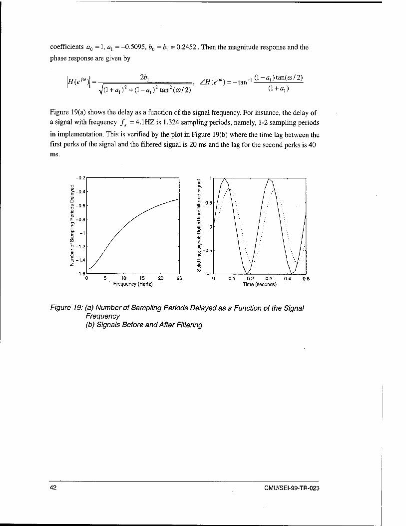
coefficients a0 = 1, a, = -0.5095, b0 = bx = 0.2452 . Then the magnitude response and the

phase response are given by

H{e'm) 2b,

•N/(l + a,)2+(l-a1)2tan2(6;/2)

, ZH(Q = -tan-l(1-*')tan(6J/2)

(1 + a,)

Figure 19(a) shows the delay as a function of the signal frequency. For instance, the delay of a signal with frequency fs = 4.1HZ is 1.324 sampling periods, namely, 1-2 sampling periods

in implementation. This is verified by the plot in Figure 19(b) where the time lag between the first perks of the signal and the filtered signal is 20 ms and the lag for the second perks is 40 ms.

5 10 15 20 Frequency (Hertz)

25 0.2 0.3 0.4 Time (seconds)

0.5

Figure 19: (a) Number of Sampling Periods Delayed as a Function of the Signal Frequency (b) Signals Before and After Filtering


REPORT DOCUMENTATION PAGE Form Approved OMB No. 0704-0188

VA 22202-4302, and lo the Office of Management and Budget. Paperwork Reduction Project (0704-0188), Washington, DC 20503.

AGENCY USE ONLY (LEAVE BLANK) REPORT DATE

November 1999

4. TITLE

A Case Study on Analytical Analysis of the Inverted Pendulum Real-Time Control System AUTHOR(S)

Seto, Danbing

Sha, Lui

7. PERFORMING ORGANIZATION NAME(S) AND ADDRESS(ES)

Software Engineering Institute Carnegie Mellon University Pittsburgh, PA 15213

9. SPONSORING/MONITORING AGENCY NAME(S) AND ADDRESS(ES)

HQ ESC/DIB 5 Eglin Street Hanscom AFB, MA 01731-2116

REPORT TYPE AND DATES COVERED

Final FUNDING NUMBERS

C —F19628-95-C-0003

PERFORMING ORGANIZATION REPORT NUMBER

CMU/SEI-99-TR-023

10. SPONSORING/MONITORING AGENCY REPORT NUMBER

12.A DISTRIBUTION/AVAILABILITY STATEMENT

Unclassified/Unlimited, DTIC, NTIS

11. SUPPLEMENTARY NOTES

12.B DISTRIBUTION CODE

13. ABSTRACT (MAXIMUM 200 WORDS)

An inverted pendulum has been used as the controlled device in a prototype real-time control system employing the Simplex™ architecture. In this report, we address the control issues of such a system in an analytic way In particular, an analytic model of the system is derived; control algorithms are designed for the baseline control, experimental control and safety control based on the concept of analytic redundancy; the safety region is obtained as the stability region of the system under the safety control; and the control switching logic is established to provide fault tolerant functionality. Finally, the results obtained and the lessons learned are summarized, and future work is discussed.

14. SUBJECT TERMS

analytic redundancy, fault tolerance, linear matrix inequality, Lyapunov function, real-time control, Simplex architecture

17. SECURITY CLASSIFICATION OF REPORT

UNCLASSIFIED

18. SECURITY CLASSIFICATION OF THIS PAGE

UNCLASSIFIED

19. SECURITY CLASSIFICATION OF ABSTRACT

UNCLASSIFIED

15. NUMBER OF PAGES

42 pp.

16. PRICE CODE

20. LIMITATION OF ABSTRACT

UL NSN 7540-01-280-5500

Standard Form 298 (Rev. 2-89) Prescribed by ANSI Std. Z39-1B 29B-102

Documents

A Case Study on Analytical Analysis of the Inverted