A case study of Western Bug - Technische Universit¤t Dresden

Dresden University of Technology

Faculty of Forest Geo and Hydro Sciences

Quantification of water and nutrient flows on a river catchment scale under scarce data conditions

(A case study of Western Bug river basin Ukraine)

Tatyana Terekhanova

Thesis is submitted in partial fulfillment of the examination requirements for the academic degree of Master of Science in Hydro Science and Engineering

(MSc HS amp E)

Supervisors Dr-Ing Jens Traumlnckner Dipl-Ing Bjoumlrn Helm Institute of Urban Water Management TU-Dresden Germany Responsible Professor Prof Dr Sctechn Peter Krebs Institute of Urban Water Management TU-Dresden Germany Lending admitted not admitted TU-Dresden Germany Chairman of Examination Commission Dresden November 2009

Declaration

This is my original work and has not been submitted for a degree award in any other University

___________________________

Tatyana Terekhanova

Born 9th August 1984

This thesis has been submitted for examination with our approval as the University Supervisors

____________________________

Dipl-Ing Bjoumlrn Helm

____________________________

Dr-Ing Jens Traumlnckner

____________________________

Prof Dr Sctechn Peter Krebs

Acknowledgement

Herewith I would like to thank the German Academic Exchange Service (DAAD) for the support of my study in Germany through a generous two year scholarship This study opened for me new horizons in my subject and gave the chance to get to know many highly-qualified and experienced colleagues in Hydro sciences from all over the world

I am very grateful to ProfDrPeter Krebs for having accepted me as his student I appreciate very much Dr Jens Traumlnckner for his comprehensive support advices and inspiration given to me while the compilation of this thesis My deepest gratitude goes to Bjoumlrn Helm for his encyclopedic help in process of data acquisition organizational issues and readiness to reply to my questions

I thank very much the staff members of the German Leibniz-Institute of Freshwater Ecology and Inland Fisheries in particularly DrMarkus Venohr and DiplPhys Dietmar Opitz for the cooperation in set up of the model I am also very grateful to the IWAS-Ukraine project team and their Ukrainian partners for the help in data acquisition

For the opportunity to study permanent support and encouragement I am deeply thankful to my great parents

Abstract

This thesis describes the set-up of mass flow analysis on river basin scale The water and nutrient matter flows were estimated for the WBug basin (Ukraine) with the application of the evaluation tool MONERIS The model was chosen due to such criteria as medium complexity of the processes description and low input data requirements In order to estimate the influence of the data availability on the MFA set up with MONERIS two data sets were applied which differed in accuracy of such input data as land cover amount of precipitations N-surplus and P-accumulation in agricultural areas river network length One set of data is characterized as ldquolocalrdquo and another is ldquoremoterdquo due to origin from Ukrainian and other information sources correspondingly

The model was run in annual time resolution for a watershed WBug ndash Kamianka-Bugska which was divided into 16 sub-catchments The modeling period corresponds to 1995 ndash 1998 for which the model validation data were available Additionally the option of MONERIS to calculate nutrient loads for design years (ldquolong-termrdquo dry and wet year) was used The validation of the modeling results has shown better fit of the water and matter flows estimated with ldquolocalrdquo data set for the ldquolong-termrdquo design year with reference ldquolong-termrdquo load values The major part of the estimated nitrogen loads is originated from agricultural areas and is delivered with groundwater pathway In contrast the phosphorous load is coming mainly from the communal WWTP and delivered accordingly with point sources

Comparison of the modeling results performed with two data sets has shown strong dependence of the model on the accuracy of land cover information especially nitrogen load estimations in comparison to phosphorous loads which calculation approach is strongly parameterized in the model The evaluation of sensitivity and uncertainty of the modeling results was performed qualitatively due to the fact that the model was not available for additional runs For the estimation of parameter sensitivity of the Urban system pathway of MONERIS the pathway was reproduced after MONERIS approach description

Such issues as influence of different input data on modeling results modeling results of MONERIS application of the quantification tool on WBug basin conditions possible remediation measures are discussed Recommendations for further model development data acquisition in the WBug basin and remediation of the nutrient loads are given

The thesis includes 80 pages with 18 tables 54 figures 63 references

In Annexes - 2 figures - 10 tables

Table of content

Abbreviations and Acronymshelliphelliphelliphelliphelliphelliphelliphelliphelliphelliphelliphelliphelliphelliphelliphelliphelliphelliphelliphelliphelliphelliphelliphellip ii List of figureshelliphelliphelliphelliphelliphelliphelliphelliphelliphelliphelliphelliphelliphelliphelliphelliphelliphelliphelliphelliphelliphelliphelliphelliphelliphelliphelliphelliphelliphellip iv List of tableshelliphelliphelliphelliphelliphelliphelliphelliphelliphelliphelliphelliphelliphelliphelliphelliphelliphelliphelliphelliphelliphelliphelliphelliphelliphelliphelliphelliphelliphellip

1 Introductionhelliphelliphelliphelliphelliphelliphelliphelliphelliphelliphelliphelliphelliphelliphelliphelliphelliphelliphelliphelliphelliphelliphelliphelliphelliphelliphelliphelliphelliphellip 1 11 Problem descriptionhelliphelliphelliphelliphelliphelliphelliphelliphelliphelliphelliphelliphelliphelliphelliphelliphelliphelliphelliphelliphelliphelliphellip 1 12 Objectiveshelliphelliphelliphelliphelliphelliphelliphelliphelliphelliphelliphelliphelliphelliphelliphelliphelliphelliphelliphelliphelliphelliphelliphelliphelliphelliphellip 3 2 Mass Flow Analysis on river basin scale literature reviewhelliphelliphelliphelliphelliphelliphelliphelliphelliphelliphellip 4 21 General concept of MFAhelliphelliphelliphelliphelliphelliphelliphelliphelliphelliphelliphelliphelliphelliphelliphelliphelliphelliphelliphelliphelliphellip 4 22 MFA for river basin scalehelliphelliphelliphelliphelliphelliphelliphelliphelliphelliphelliphelliphelliphelliphelliphelliphelliphelliphelliphelliphellip 5 221 Specific properties of matter flows in river basinhelliphelliphelliphelliphelliphelliphelliphelliphellip 5 222 Nutrients sources transformation processes and sinkshelliphelliphelliphelliphelliphelliphellip 8 2221 Cycling of Nitrogenhelliphelliphelliphelliphelliphelliphelliphelliphelliphelliphelliphelliphelliphelliphelliphelliphellip 8 2222 Cycling of Phosphoroushelliphelliphelliphelliphelliphelliphelliphelliphelliphelliphelliphelliphelliphelliphellip 11 23 Available models and tools for Nutrients Flow Analysis on river basin scalehellip 13 231 Types of modelshelliphelliphelliphelliphelliphelliphelliphelliphelliphelliphelliphelliphelliphelliphelliphelliphelliphelliphelliphelliphelliphellip 13 232 Existing mass balance models and tools for river basin scale and their

evaluationhelliphelliphelliphelliphelliphelliphelliphelliphelliphelliphelliphelliphelliphelliphelliphelliphelliphelliphelliphelliphelliphelliphelliphelliphelliphelliphellip 15 233 MONERIS (Modeling of Nutrient Emissions in River System)helliphelliphelliphellip 19 3 Methodologyhelliphelliphelliphelliphelliphelliphelliphelliphelliphelliphelliphelliphelliphelliphelliphelliphelliphelliphelliphelliphelliphelliphelliphelliphelliphelliphelliphelliphellip 23 31 Study case Western Bug river basinhelliphelliphelliphelliphelliphelliphelliphelliphelliphelliphelliphelliphelliphelliphelliphelliphellip 23 32 Model set uphelliphelliphelliphelliphelliphelliphelliphelliphelliphelliphelliphelliphelliphelliphelliphelliphelliphelliphelliphelliphelliphelliphelliphelliphelliphelliphellip 30 33 Data acquisition and related calculationshelliphelliphelliphelliphelliphelliphelliphelliphelliphelliphelliphelliphelliphelliphelliphellip 31 331 Basic informationhelliphelliphelliphelliphelliphelliphelliphelliphelliphelliphelliphelliphelliphelliphelliphelliphelliphelliphelliphelliphelliphellip 32 332 Time series data (ldquoPeriodical datardquo)helliphelliphelliphelliphelliphelliphelliphelliphelliphelliphelliphelliphelliphellip 43 333 Individual WWTPshelliphelliphelliphelliphelliphelliphelliphelliphelliphelliphelliphelliphelliphelliphelliphelliphelliphelliphelliphelliphellip 47 334 Country datahelliphelliphelliphelliphelliphelliphelliphelliphelliphelliphelliphelliphelliphelliphelliphelliphelliphelliphelliphelliphelliphelliphellip 47 335 Measured runoff and nutrient loadshelliphelliphelliphelliphelliphelliphelliphelliphelliphelliphelliphelliphelliphellip 48 34 Validation of the model resultshelliphelliphelliphelliphelliphelliphelliphelliphelliphelliphelliphelliphelliphelliphelliphelliphelliphelliphellip 49 341 Model precisionhelliphelliphelliphelliphelliphelliphelliphelliphelliphelliphelliphelliphelliphelliphelliphelliphelliphelliphelliphelliphelliphellip 49 342 Model accuracyhelliphelliphelliphelliphelliphelliphelliphelliphelliphelliphelliphelliphelliphelliphelliphelliphelliphelliphelliphelliphelliphellip 51 35 Sensitivity analysishelliphelliphelliphelliphelliphelliphelliphelliphelliphelliphelliphelliphelliphelliphelliphelliphelliphelliphelliphelliphelliphelliphelliphellip 52 351 Response of the model on ldquolocalrdquo and ldquoremoterdquo data setshelliphelliphelliphelliphelliphellip 52 352 MONERIS - Urban Systemhelliphelliphelliphelliphelliphelliphelliphelliphelliphelliphelliphelliphelliphelliphelliphelliphelliphellip 56 36 Uncertainty analysishelliphelliphelliphelliphelliphelliphelliphelliphelliphelliphelliphelliphelliphelliphelliphelliphelliphelliphelliphelliphelliphelliphelliphellip 60 361 Uncertainty in input datahelliphelliphelliphelliphelliphelliphelliphelliphelliphelliphelliphelliphelliphelliphelliphelliphelliphelliphellip 61 362 Uncertainty in modelinghelliphelliphelliphelliphelliphelliphelliphelliphelliphelliphelliphelliphelliphelliphelliphelliphelliphelliphellip 62 4 Results and Discussionhelliphelliphelliphelliphelliphelliphelliphelliphelliphelliphelliphelliphelliphelliphelliphelliphelliphelliphelliphelliphelliphelliphelliphelliphellip 64 41 Evaluation of modeling Resultshelliphelliphelliphelliphelliphelliphelliphelliphelliphelliphelliphelliphelliphelliphelliphelliphelliphellip 64 42 Application of scenarioshelliphelliphelliphelliphelliphelliphelliphelliphelliphelliphelliphelliphelliphelliphelliphelliphelliphelliphelliphelliphellip 70 43 Discussionhelliphelliphelliphelliphelliphelliphelliphelliphelliphelliphelliphelliphelliphelliphelliphelliphelliphelliphelliphelliphelliphelliphelliphelliphelliphelliphellip 71 5 Conclusions and Recommendationshelliphelliphelliphelliphelliphelliphelliphelliphelliphelliphelliphelliphelliphelliphelliphelliphelliphelliphelliphellip 74 51 Conclusionshelliphelliphelliphelliphelliphelliphelliphelliphelliphelliphelliphelliphelliphelliphelliphelliphelliphelliphelliphelliphelliphelliphelliphelliphelliphellip 74 52 Recommendationshelliphelliphelliphelliphelliphelliphelliphelliphelliphelliphelliphelliphelliphelliphelliphelliphelliphelliphelliphelliphelliphelliphelliphellip 75 Referenceshelliphelliphelliphelliphelliphelliphelliphelliphelliphelliphelliphelliphelliphelliphelliphelliphelliphelliphelliphelliphelliphelliphelliphelliphelliphelliphelliphelliphelliphelliphellip

Annexeshelliphelliphelliphelliphelliphelliphelliphelliphelliphelliphelliphelliphelliphelliphelliphelliphelliphelliphelliphelliphelliphelliphelliphelliphelliphelliphelliphelliphelliphelliphelliphellip 81

Abbreviations and Acronyms

Description Unit a Substance in input good ABAG General Soil Losses Equation (Algemeine Boden Abtrag

Gleichnung)

ADdir_prec Runoff from precipitation falling directly on surface runoff [m3s] Aopm Areas with open mining [km2] ASR_snow Snow covered area [km2] ATD Tile drained areas [km2] AtotalAU Total area of sub-basin [m3s] ATV - DVWK Abwassertechnische Vereinigung fuer Wasserwirtschaft

Abwasser und Abfall

b Substance in output good BOD5 Biological Oxygen Demand within 5 days BSDB Baltic Sea Drainage basin c Concentration [kgm3] CLC CORINE land cover COD Chemical Oxygen Demand CORINE Coordination on Information on the Environment CSO Combined Sewer Overflow DEM Digital Elevation Model DIN Dissolved Inorganic Nitrogen DWD German Weather Service ECA European Climate Assessment ESRI Environmental System Research Institute EU European Union EUROHARP Project ldquoTowards European Harmonized Procedures for

Quantification of Nutrient Losses from Diffuse Sources

EWFD European Water Framework Directive FAO-UNOFAO Food and Agricultural Organization of the United Nations GIS Geographical information system GPCC The Global Precipitation Climatology Centre IDW Inverse Distance weighted interpolation IGB German Leibniz-Institute of Freshwater Ecology and Inland

Fisheries

IHM TUD Institute for Hydrology and Meteorology of the Dresden University of Technology

ISI TUD Institute for industrial and urban water management of the Dresden University of Technology

IWAS - Ukraine International Water Alliance Saxony model region Ukraine IWRM Integrated Water Resources Management KGWRA1 Area of groundwater renewal [km2] ki Transfer coefficient L Matter load [kg] MFA Material Flow Analysis MONERIS Modeling of Nutrient Emissions in River system N Nitrogen NASA-SRTM National Aeronautics and Space Administration - Shuttle Radar

Topography Mission

NM Nutrient matter NOAA National Oceanic and Atmospheric Administration Ntotal Total nitrogen P Phosphorous PELCOM Pan-European Land Cover Monitoring Q Water discharge [m3s] QGW Ground water flow [m3s] qHL Specific runoff-Hydraulic Load approach QPD_calc Runoff as input variable in periodical data [m3s] Qsr Runoff of surface flow [m3s] QTD Runoff from tile drained areas [m3s] Qus Runoff from urban areas [m3s] SWAT Soil and Water Assessment Tool SWECO Swedish Engineering Company TACIS ldquoTechnical Aid to the Commonwealth of Independent Statesrdquo

program

THL Temperature-Hydraulic Load approach TKN Total Kjeldahl Nitrogen TN Total nitrogen TP Total phosphorous TPE-1d-1 Total phosphorous pro Inhabitant per day [g] TRB Transboundary River Basins USA United States of America USDA United States Department of Agriculture USIAU_total Impervious urban area in sub-basin [km2] USSR United Socialistic Soviet Republics WBug Western Bug WBBA State Western Bug river Basin Authority WSAmrtrib Surface area of the entire river network [km2] WWTP Waste water treatment plant

List of Figures

Figure 21 Natural water cyclehelliphelliphelliphelliphelliphelliphelliphelliphelliphelliphelliphelliphelliphelliphelliphelliphelliphelliphelliphelliphelliphellip 6 Figure 22 Main chemical transformations of nitrogen compoundshelliphelliphelliphelliphelliphelliphelliphellip 9 Figure 23 Overview of main nitrogen sinks and sources within river basinhelliphelliphelliphellip 9 Figure 24 Overview of sources and sinks of phosphoroushelliphelliphelliphelliphelliphelliphelliphelliphelliphelliphellip 12 Figure 25 A general relation between the complexity of models (left) model type

(right) and the generated outputhelliphelliphelliphelliphelliphelliphelliphelliphelliphelliphelliphelliphelliphelliphelliphelliphellip

14 Figure 26 Modeled specific nitrogen input from agricultural lands in relation to mean

value of modelinghelliphelliphelliphelliphelliphelliphelliphelliphelliphelliphelliphelliphelliphelliphelliphelliphelliphelliphelliphelliphelliphelliphellip

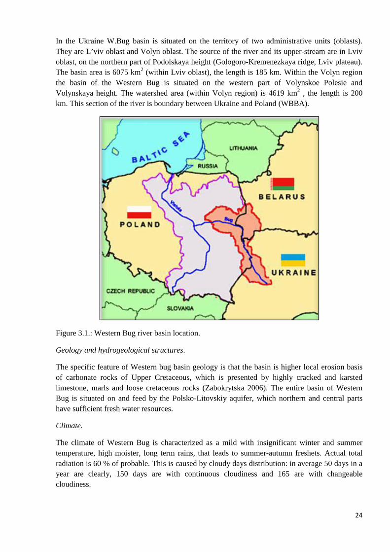
17 Figure 27 Conceptual scheme of MONERIShelliphelliphelliphelliphelliphelliphelliphelliphelliphelliphelliphelliphelliphelliphelliphellip 20 Figure 31 Western Bug river basin locationhelliphelliphelliphelliphelliphelliphelliphelliphelliphelliphelliphelliphelliphelliphelliphelliphellip 24 Figure 32 Water use in Western Bug basin in 2001helliphelliphelliphelliphelliphelliphelliphelliphelliphelliphelliphelliphelliphellip 28 Figure 33 Long-term concentrations of TN and TP in WBug basinhelliphelliphelliphelliphelliphelliphellip 29 Figure 34 Division of WBug-Kamianka-Bugska basin into sub-catchmentshelliphelliphelliphellip 31 Figure 35 Mean annual value of NHx atmospheric deposition on WBug river basin in

1980-2000helliphelliphelliphelliphelliphelliphelliphelliphelliphelliphelliphelliphelliphelliphelliphelliphelliphelliphelliphelliphelliphelliphelliphelliphelliphellip 32

Figure 36 Evapotranspiration in WBug - Kamianka-Bugska catchmenthelliphelliphelliphelliphelliphellip 33 Figure 37 Digital elevation model of WBug ndash Kamianka-Bugskahelliphelliphelliphelliphelliphelliphelliphellip 33 Figure 38 Total agricultural production in Lviv oblast Ukrainehelliphelliphelliphelliphelliphelliphelliphelliphellip 34 Figure 39 Soil types in WBug river basin due to Russian Soil Classificationhelliphelliphelliphellip 35 Figure 310 Distribution of different soil textures in WBug river basinhelliphelliphelliphelliphelliphelliphellip 36 Figure 311 Land use in WBug basin after CLC amp PELCOMhelliphelliphelliphelliphelliphelliphelliphelliphelliphellip 37 Figure 312 Comparison of topographic map with digital map of river networkhelliphelliphellip 38 Figure 313 Estimated drained areas in WBug river basinhelliphelliphelliphelliphelliphelliphelliphelliphelliphelliphelliphellip 39 Figure 314 Generated river network on DEM90 of WBug river basinhelliphelliphelliphelliphelliphelliphellip 39 Figure 315 Scheme of the meteorological stations surrounding WBug basin which

data are included in NOAA and ECA data baseshelliphelliphelliphelliphelliphelliphelliphelliphelliphelliphellip

40 Figure 316 Regression relation between ECA and NOAA precipitation valueshelliphelliphellip 41 Figure 317 Annual amount of precipitations for 1980-2007 in WBug basin

interpolated with IDWhelliphelliphelliphelliphelliphelliphelliphelliphelliphelliphelliphelliphelliphelliphelliphelliphelliphelliphelliphelliphellip 42

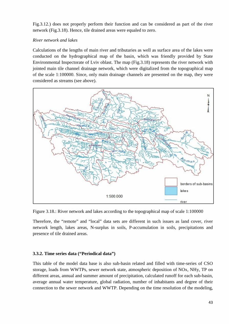
Figure 318 River network and lakes according to the topographical maphelliphelliphelliphelliphelliphellip 43 Figure 319 Scheme of WWTPs in WBug ndash Kamianka-Bugska catchmenthelliphelliphelliphelliphellip 45 Figure 320 Annual precipitations (mm) in 1995 in WBug basinhelliphelliphelliphelliphelliphelliphelliphelliphellip 46 Figure 321 Mean month water temperature (degC) in WBug riverhelliphelliphelliphelliphelliphelliphelliphelliphellip 47 Figure 322 Annual water discharge in WBug-Kamianka-Bugska for 1968-1998helliphellip 48 Figure 323 Measured vs calculated in MONERIS water discharge in WBughelliphelliphelliphellip 49 Figure 324 Measured vs calculated TN and TP loads for WBughelliphelliphelliphelliphelliphelliphelliphelliphellip 50 Figure 325 Long-term TN and TP loadhelliphelliphelliphelliphelliphelliphelliphelliphelliphelliphelliphelliphelliphelliphelliphelliphelliphelliphellip Figure 325 TN and TP measured loads vs MONERIS loads in long-term conditionshellip 50 Figure 326 TN and TP measured loads vs MONERIS loads in log-scalehelliphelliphelliphelliphelliphellip 51 Figure 327 Areas with different land cover in ldquolocalrdquo and ldquoremoterdquo data setshelliphelliphelliphellip 52 Figure 328 Total river lengths in sub-basins of WBug helliphelliphelliphelliphelliphelliphelliphelliphelliphelliphelliphelliphellip 53 Figure 329 Calculated runoff separation for ldquolocalrdquo and ldquoremoterdquo data setshelliphelliphelliphelliphellip 54 Figure 330 TN and TP inputs from different pathways for ldquolocalrdquo and ldquoremoterdquo data hellip 55 Figure 331 Retention in tributaries vs total river network lengthshelliphelliphelliphelliphelliphelliphelliphellip 56 Figure 332 MONERIS concept of the calculation of nutrients load from urban areashellip 57 Figure 333 MONERIS ldquolocalrdquo urban system runoff (Qus) vs Runoff (Qus)

ldquoMONERIS - Urban systemrdquohelliphelliphelliphelliphelliphelliphelliphelliphelliphelliphelliphelliphelliphelliphelliphelliphelliphellip 58

Figure 334 TN and TP Loads partitioning between urban sources helliphelliphelliphelliphelliphelliphelliphellip 58 Figure 335 MONERIS ldquolocalrdquo TN and TP Urban System loads vs TN and TP loads

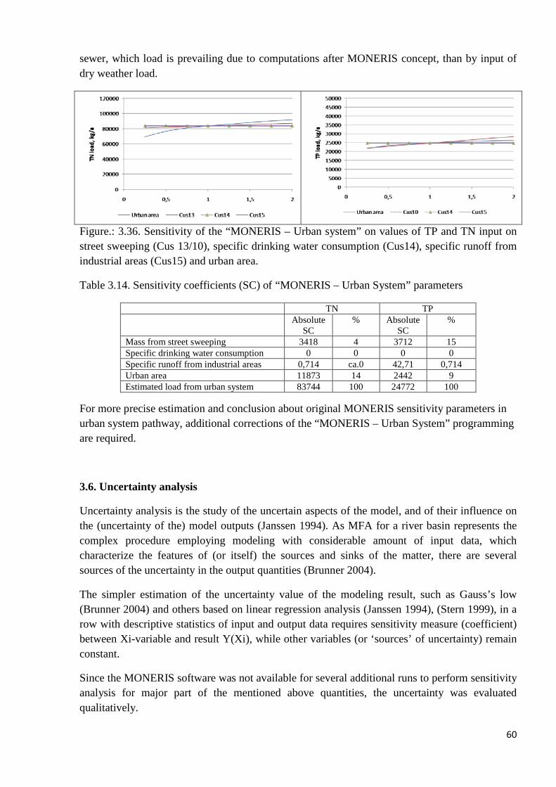
Figure 336 Sensitivity of the ldquoMONERIS ndash Urban systemrdquo on values of TP and TN input from street sweeping specific drinking water consumption specific runoff from industrial areas and urban areahelliphelliphelliphelliphelliphelliphelliphelliphelliphelliphelliphelliphellip

Figure 337 Comparison of applied and official factual TN and TP loads from WWTPs 62 Figure 41 Runoff separation in WBug basin due to MONERIS pathways and

hydrograph of WBug ndashKamianka-Bugska in 1992helliphelliphelliphelliphelliphelliphelliphelliphelliphellip 64

Figure 42 TN (left) and TP (right) sources apportioning in WBug river basin for long-term conditionshelliphelliphelliphelliphelliphelliphelliphelliphelliphelliphelliphelliphelliphelliphelliphelliphelliphelliphelliphelliphelliphellip

Figure 43 TN apportioning among sub-basins and TN distribution among sources in sub-basinshelliphelliphelliphelliphelliphelliphelliphelliphelliphelliphelliphelliphelliphelliphelliphelliphelliphelliphelliphelliphelliphelliphelliphelliphelliphellip

Figure 44 TP apportioning among sub-basins and TP distribution among sources in sub-basinshelliphelliphelliphelliphelliphelliphelliphelliphelliphelliphelliphelliphelliphelliphelliphelliphelliphelliphelliphelliphelliphelliphelliphelliphelliphellip

Figure 45 TN and TP inputs from different pathways for entire WBug basinhelliphelliphellip 67 Figure 46 TN and TP inputs from different pathways in sub-basins of WBughelliphelliphellip 67 Figure 47 Specific total TN (kgha) and TP (gha) input from sub-basinshelliphelliphelliphelliphellip 68 Figure 48 TN and TP retention () in tributaries of WBug in long-term periodhelliphellip 69 Figure 49 NM retention in ldquomain riverrdquo for sub-basins of WBughelliphelliphelliphelliphelliphelliphelliphellip 69 Figure 410 Resulting TN and TP loads for WBug basin (tonesa)helliphelliphelliphelliphelliphelliphelliphellip 70

List of tables

Table 21 Terms and definitions in Material Flow Analysishelliphelliphelliphelliphelliphelliphelliphelliphelliphellip 4 Table 22 Characteristic of model types for process descriptionhelliphelliphelliphelliphelliphelliphelliphelliphellip 14 Table 23 Quantification tools and their application cases within EUROHARPhelliphelliphellip 16 Table 24 Evaluation of model applicability on Western Bug river basinhelliphelliphelliphelliphellip 18 Table 31 Accordance of MONERIS set up to MFA procedurehelliphelliphelliphelliphelliphelliphelliphelliphellip 23 Table 32 Main climate characteristics of WBug basinhelliphelliphelliphelliphelliphelliphelliphelliphelliphelliphelliphellip 25 Table 33 Mean annual water runoff characteristicshelliphelliphelliphelliphelliphelliphelliphelliphelliphelliphelliphelliphelliphellip 25 Table 34 Seasonal nutrients load from Ukrainian part of WBug basin (1989ndash2003) 29 Table 35 Annual and seasonal Nutrients load (1989 ndash 2003)helliphelliphelliphelliphelliphelliphelliphelliphelliphelliphelliphelliphellip 29 Table 36 Characteristics of raster images of soil losses from areas with different land

coverhelliphelliphelliphelliphelliphelliphelliphelliphelliphelliphelliphelliphelliphelliphelliphelliphelliphelliphelliphelliphelliphelliphelliphelliphelliphelliphelliphellip

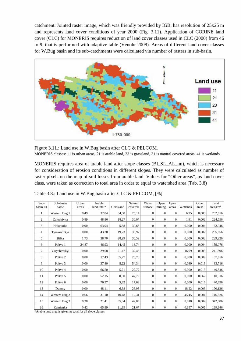
34 Table 37 Accepted soil texture typeshelliphelliphelliphelliphelliphelliphelliphelliphelliphelliphelliphelliphelliphelliphelliphelliphelliphelliphellip 36 Table 38 Land use in WBug basin after CLC amp PELCOMhelliphelliphelliphelliphelliphelliphelliphelliphelliphellip 37 Table 39 Correlation coefficients for the supplement of precipitation time-serieshelliphellip 41 Table 310 Nutrient load for WBug ndash Kamianka-Bugskahelliphelliphelliphelliphelliphelliphelliphelliphelliphelliphelliphellip 48 Table 311 Nutrient matter concentrations for WBug basinhelliphelliphelliphelliphelliphelliphelliphelliphelliphellip 51 Table 312 Total NM input for ldquolocalrdquo and ldquoremoterdquo data setshelliphelliphelliphelliphelliphelliphelliphelliphelliphellip 54 Table 313 Variables and model parameters used in sensitivity analysishelliphelliphelliphelliphelliphellip 59 Table 314 Sensitivity coefficients (SC) of ldquoMONERIS ndash Urban Systemrdquo parametershellip 60

1 Introduction

The concept of Integrated Water Resources Management (IWRM) based on an overall consideration of the water cycle its compartments and interrelated processes seems to be a promising solution for existing worldwide water resources problems IWRM is aimed to propose water management solutions which could minimize harmful anthropogenic influences on waters and secure sustainable water economy within changing environmental socio-economical and technological conditions (Grambow 2007)

Obviously implementation of this concept in practice requires appropriate knowledge about water cycle and its interrelations with other parts of geosphere within a certain spatial unit Hence there is rising necessity of quantitative and qualitative description of not only cycle of water resources but also of all nature and anthropogenic conditions through which water goes

Regarding water quality such description can be implemented by engaging Material Flow Analysis (MFA) as quantification tool for sources pathways and sinks of substances MFA for river basin due to exceptional water feature as carrier of matter is based on the water balance approach

Therefore MFA for river basin with regard to water quality estimation represents balance of substances carried with water to the outlet Set up of such balance allows to make water management integrated decisions appropriate to the certain objectives

11 Problem description

Since year 2000 when European Water Framework Directive (EWFD) entered into force all the Members of European Community are obliged to perform their activities influencing on water resources within the definitions of Integrated Water Resource Management (EWFD) Special emphasis of the Directive 200060EC is given to environmental objectives due to article 41 Member States shall prevent deterioration of the status of all surface water bodies and achieve good ecological potential and good chemical surface water status (EWFD)

As far as EWFD concerns not only surface water objects but also groundwater aquifers and territorial and marine water (EWFD) intern European seas are in special consideration such as Baltic Sea Major part of river basin feeding Baltic Sea belongs to international (transboundary) river basins Regarding transboundary rivers environmental objectives established under mentioned Directive should be coordinated for the whole of the river basin district

The comparative analysis of transboundary river basins of Baltic Sea after such indicators as water quality and degree of cooperation between countries for basin management performed by Nilsson (2006) has shown that Vistula Pregolya and Neman are the three most ldquocriticalrdquo international river basins in the Baltic sea drainage basin (Nilsson 2006) Regarding point of water quality in that analysis it seems to be less significant due to the map of anthropogenic modification these rivers are not the worse cases in Europe (WRc 2007) there are only 5 ndash 20 of heavily modified and artificial water bodies

Another point is that all these basins are partly occupied by former Soviet Union countries It could mean that in spite of the fact that some countries have already become EU members the systems of water resources management and control are still keeping ldquosoviet standardsrdquo This fact could make some format difficulties in cooperative work especially with countries such as the Ukraine and the Republic of Belarus

One of the difficulties which is met by International Water Aliance Saxony in the Project ldquoManagement of water resources in hydrological sensitive world regionsrdquo Region Ukraine is data acquisition ldquoIWAS Ukrainerdquo is a working group conducting its research on the study case of Western Bug river basin which belongs to the largest PolishVistula basin

On the Ukrainian part of WBug river basin regional administration (WBBA Bodnarchuk 2008) and scientists (Zabokrytska 2006) underlines the following water related problems

- exceeding of the limit permissible concentration of pollutants in the waste waters

- slow implementation of water protection zones

- reduction of the river flow cross sections due to sedimentation and littering

- flooding of settlements and agriculture objects

- required liquidation and neutralization of hazardous wastes deposits in the basin

- insufficient number of hydrological and hydrochemical observations

These problems causes the problem of water pollution in WBug river which consists in increasing of nitrate and phosphate concentrations in the river water pollution of water by organic matter and compounds from communal waste water treatment plants (WWTP) effluents industrial pollution by heavy metals and increase of total mineralization diffuse pollution by pesticides polyaromatic hydrocarbon etc (Bodnarchuk 2008)

Among others inappropriate water quality issue is under special consideration due to inflow of river into EU area where EWFD is maintained Zabokrytska et al (2006) calculated that in its outflow into the river Narew (Poland) WBug has a matter load 93 of which are originated from Ukrainian part of the basin and 7 are from Polish (Zabokrytska 2006) Furthermore almost one third of matter load of WBug on the Ukrainian-Polish state boarder originates from tributary of WBug the river Poltva (Zabokrytska et al 2006) As it is mentioned in TACIS Report (2001) discharge of the Poltva in the headwaters of Western Bug amounts to 9 m3s and 23 of which is the effluent from the waste water treatment plant from the city of Lviv the administrative centre of Lviv oblast whilst the discharge of river Bug amounts only to about 6 m3s (TACIS 2001)

Therefore severe anthropogenic influence on the water quality of WBug is considered to be main reason of water pollution Obviously in conditions of financial difficulties (WBug Basin Authority 2006) it is not possible to implement urgent reconstruction measures on WWTPs hence the pollutants sources partitioning should be defined MFA set up for a river basin can afford to find other spots of the water quality problem and based on that appropriate solutions can be found

12 Objectives

General objective

For the catchment of the river Western Bug (Ukraine) a MFA shall be set up The scarce data base demands the definition of missing parameters based on case studies with comparable natural and management conditions The sensitivity of results on uncertain parameters shall be defined

Specific objectives

1 Literature review general approach of MFA in river basin scale (relevant flows substances sources sinks and transformation processes) available models and tools (evaluation of pros and cons with regard the Western Bug study case)

2 MFA setup Definition of the system boundaries and of subcatchments quantification of main input paths (emission inventory) for Q P N and comparison with available immission data implementation in MFA using a mass transport model on river system scale and plausibility check based on available water quality data sensitivity analysis for uncertain model parameters

3 Identification of pollution sources and measures Ranking the main polluters based on the MFA and proposal of infrastructural or operational measures to reduce pollution loads

4 Scenario calculation Definition of probable and desirable development scenarios implementation of the scenarios in the MFA and evaluation of the results

5 Final evaluation of the chosen approach and proposal for adaptationimprovement with special regard to the study case

2 Mass Flow Analysis on river basin scale literature review

21 General concept of MFA

Material Flow Analysis (MFA) is a tool used for definition analysis and description of the material cycles in a system (Baccini 1996) MFA allows to quantify matter cycling in defined spatial and temporal units (system boundaries) Matter or energy balances (ie application of matter or energy conservation lows) should be set up to describe material flows within the system

MFA approach for system investigations has found its application already in 1930ths in economics (Brunner 2004) Afterwards it has been successfully using in chemical engineering (since 1960ths) as well as for investigation of agricultural lands private economies craft and industrial enterprises entire regions like countries or watersheds (Baccini 1996)

Since MFA is considered as multidisciplinary approach a certain terminology is utilized to set up the balances Main terms of the tool defined by Baccini (Baccini 1996) are substance goods processes matter cycling system and activities Brunner (Brunner 2004) represents wider list of main terms of MFA (Table 21)

Table 21 Terms and definitions in Material Flow Analysis (after (Brunner 2004)

Definition

Substance Any (chemical) element or compound composed of uniform units All substances are characterized by a unique and identical constitution and are thus homogeneous for example Nitrogen and Phosphorous

Goods Economic entities of matter with a positive or negative economic value They are made up of one or several substances for example wood waste water automobiles fertilizer etc

Material Serves as umbrella-term for substances and goods for example carbon and concrete are materials

Processes Transformation transport or storage of materials for example processes of matter cycling in human body WWTP soil body etc

Flow Ratio of mass per unit time that flows through a conductor for example water flow in pipe consumption of oil for entire system

Transfer coefficient Designates the part of total substance introduced into the process which will be transferred into output good eg kib = ba where b is for substance in output good a is for substance in input good

System A group of elements the interaction between these elements and the boundaries between these and other elements in space and time It is a group of physical components connected or related in such a manner as to form andor act as an entire unit

Activities Actions of people to satisfy their needs

Usually processes are defined as black box if it is not the case then process should be subdivided into sub-processes (Brunner 2004)

Based on described terminology Baccini and Bader (1996) presents following conceptual steps of MFA

1) choice of system which should be described in terms of goods processes and one or more substances

2) measurements or data acquisition ofabout good flows and substance concentrations in goods

3) calculation of material flows 4) schematical presentation and interpretation of results identification of sources and sinks

of matter processes and flow pathways relevant to material cycling possible management measures aiming to desirable changes in described system

Depending upon the discipline where MFA is applied the balance approach can be process related product related or substance related For environmental sciences in last decades the substance related balancing approach was widely used (Baccini 1996) Currently MFA for entire regions practically is implemented within Environmental Information Systems which include three parts Firstly it is data management and visualization which is carried via geographical information systems (GIS) Then it is a model to simulate the processes in current state and prognoses Finally it is expert systems which help to interpret and estimate the results (Baccini 1996)

Hence conceptual steps are completely covered in the practical procedure of MFA Choice of system and set up of system boundaries are determined by formulation of problem and objective of investigation Data acquisition can be organized with help of GIS Calculation of material flow and identification of main sources sinks and pathways of substances are carried out in process oriented models Consequences and results planned management measures can be evaluated employing scenario technique

Therefore as it can be seen from approach description the MFA can give detailed quantitative description of investigated system and estimation of possible consequences in case of desirableundesirable changes

22 MFA for river basin scale

221 Specific properties of matter flows in river basin

As in general case MFA for river basin scale means identification of sources pathways sinks and transformation processes of substance For such substance as water this procedure is followed in set up of water balance for a watershed (Dyck 1995) Hence a set up of water balance represents already Mass Flow Analysis for river basin scale

Since water quality formation depends on the characteristics of the medium water flows through then a set up of the MFA based on the water balance can be applied for the quantitative assessment of water quality formation process on a watershed That is valuable for water quality

management to which the MFA method was firstly applied in Europe in a Swiss river catchment (Brunner et al 1990) and on transnational scale for the Danube Basin (Somlyoacutedy et al 1997) proving to be a helpful tool for the early recognition of environmental problems and evaluation of solutions to these problems (Schaffner 2006)

Hence composition of water budget is essential part of any mass balance modeling for river basin scale

Naturally water serves as connecting medium of geosphere compartments This connection is provided via hydrologic cycle (Fig21) The hydrologic cycle can be described as the exchange of water between the earthrsquos surface and atmosphere driving by sun energy and force of gravity through processes such as condensation (cloud formation) precipitation runoff infiltration evaporation and transpiration (DeBarry 2004)

Figure 21 Natural water cycle (Source (Roussy 2006)

The amounts of water in storage and in transit at any point in time within the hydrologic cycle can be described with hydrologic or water balance The water balance is actually matter conservation law applied to water within watershed in long term condition

Inflow = outflow + change in storage (Derek Eamus 2006)

The water budget in contrast is described in the short term where inflow and outflow may not balance (DeBarry 2004)

The hydrologic cycle often refers only to the physical parameters of water although it includes many chemical and biological processes (DeBarry 2004) Water is main solvent and carrier of matter (Dyck 1995) There are three main phases of hydrologic cycle where natural processes of matter mobilization transport accumulation and transformation take place atmosphere soilground water bodies Within these phases water takes up and losses carrying matter

Many changes in natural hydrologic balance occur due to land and water alteration and urbanization by humans (DeBarry 2004) The anthropogenic changes to water balance GKovacs et al (1989) bounds with such human activities as

- Agricultural activities - Irrigation - Forest management - Extent of urban areas - Water supply and waste water disposal - Rapid removal of rainwater and flood control - Landscape manipulation and diversity of urban areas - Mining and Quarries

Moreover the interruption of natural water cycle is determined by the stage of the water management in the basin (Kovacs 1989) The anthropogenic disturbances of water balance automatically interrupt natural processes of transformation transport and storage of substances Therefore matter flow analysis within a river basin should consider as geogenic as well as anthropogenic factors of water quality formation

Another important feature of matter flows in river basin is spatial character and their location specific values To overcome that Geo Information Systems (GIS) or their logic are applied (Brunner et al 2004Baccini 1996)

Spatial character of variables causes the problem of sufficient spatial resolution As far as river basin scale can be considered in different dimensions macro- meso- microscale (Dyck 1995) applied spatial resolution should answer the purposes of investigation type of applied process model and available data (Plate 2008) The same is true for time resolution which also depends on scales of investigated or involved processes and data availability (Plate 2008)

The experience of mass flow modeling for river basins has variety of examples of MFA application from small watersheds in micro scale like in (Schaffner 2006) (Correll 1981) (Hejzlar 1996) where balancing is performed based on field measurements to huge transboundary river systems like Danube or Rhine (de Wit 2001) (Behrendt 1999) Tisza Project (Tisza 2004)(Kaul 2008) in which case simulation of processes in related scale and GIS application for appropriate data management are desirable

A plenty of investigation of MFA is done for European river basins (all scales) in order to exactly indentify causes of water quality problems and find appropriate solutions aiming to follow EWFD (Biegel 2006) One example of such European wide projects is Project EUROHARP where 8 different nutrients flow models were applied for 17 Europe wide catchments (Silgram 2004) Another group of investigations is performed in order to estimate influence of European river discharges on seas pollution (Wittgren 1996) (Nilsson 2006) Assessment of water quality of Transboundary Rivers also can be marked as typical case of MFA application on river basin scale (Tisza project (2004)(Somlyody 1999)

Regarding data requirements for MFA on the one hand it is stated that key advantages of MFA lie in its potential to capitalize on available data and knowledge instead of investing in cost- and resource ndashintensive data assessment and modeling (conventional river water quality models)

(Schaffner 2006) On the other hand it is underlined that one of the problems researchers met while setting up of the MFA is data availability Especially the scarcity of data is noted in developing countries (Falkenmark 1989) where data acquisition is complicated due to different reasons Nevertheless required amount of data and their scarcity depend on applied methodology and particular study case (Plate 2008)

222 Nutrients sources transformation processes and sinks

Nutrients are the chemicals constructing life matter and supporting bio-chemical processes of ecosystems Such nutrients as Phosphorus and Nitrogen and their compounds have special meaning for water ecology First of all in conditions of nutrients surplus and certain PN ratio they push up primary production that leads to eutrophication (Ryding 1990) Increase of biological activity decreases oxygen content which among other consequences brakes oxidation and in particular denitrification processes This forms undesirable water quality as for water fauna (ammonia is acute toxic for fishes) as well as for water use especially for drinking water supply purposes (Voss 2007)

In natural undisturbed environments the nutrient supply is derived from the drainage of a catchment together with direct rainfall on the water surface and any internal recycling which may occur from the sediments Based on the results of studies which have been made upon such catchments Harper (1992) has shown that nutrient runoff is very low because the cycling within the vegetation of the terrestrial ecosystem is very tight (true for entire forested catchments) In the temperate zones nutrient runoff from different areas decreases in following order arable land natural or secondary grassland forested land Urban areas produce a range of high-nutrient effluents but their contribution depends on the urbanization degree of watershed (Harper 1992) The same order of nitrogen sources is presented by RLiden et al (1999) for Matsalu Bay watershed (Estonia)

2221 Cycling of Nitrogen

The main source of nitrogen on the Earth is the atmospheric reservoir of gaseous nitrogen Nitrogen gas is chemically very stable but is made available to organisms by fixation into a variety of oxides or reduction to ammonium The most important inorganic forms of nitrogen are ammonia (NH3) nitrite (NO2

-) nitrate (NO3-) and molecular nitrogen (N2) Simplified

transformations of nitrogen and its compounds can be described with six major processes as illustrated below on Figure 22

Diffuse sources of Nitrogen in river basin

Due to the fact that nitrogen fixation by microorganisms in the soil is about seven times greater than nitrogen from all atmospheric processes brought to earth by rainfall (Harper 1992) soil solution and soil erosion are to be considered main sources of nitrogen and its compounds in water bodies

(1) Assimilation of inorganic-N by microorganisms and plants to form organic-N such as proteins and amino acids (2) Heterotrophic conversions involving the transfer of organic N among organisms (3) Ammonification the breakdown of organic-N to NH3-N by bacteria and fungi (4) Nitrification the microbial mediated oxidation of NH3-N to NO2-N and NO3-N (5) Denitrification the microbial mediated production of NO2-N and N2 in anaerobic conditions (6) Biological nitrogen fixation conversion of N2 to NH3-N

Figure 22 Main chemical transformations of nitrogen compounds

Main processes of nitrogen transport and transformation in soils are described by Scheffer and Schachtschabel (2002) in detail Input of nitrogen and its compounds into soil is realized through organic and inorganic fertilizers irrigation atmospheric deposition decomposition of plant residuals and biological N2- fixation Output is presented by plants uptake wash out soil erosion NH3 ndash volatilization denitrification ammonia-fixation and N2- fixation (Fig23)

Figure 23 Overview of main nitrogen sinks and sources within river basin

A significant source of nitrogen (especially in vegetation pause) in soils is fertilizers brought on arable land Fertilizer can contain as organic nitrogen (manure compost etc) as well as mineral nitrogen (anhydrous ammonium nitrate urea) The amount of applied fertilizer depends on soil properties type of crop type of fertilizer environmental regulations of country level of agriculture development etc (Schilling 2000)

As it was mentioned above there are two main possibilities for nitrogen and its compounds to enter water body They are soil water solution and erosion (Voss 2007) Nitrate due to its high solubility will be transferred mainly in solution One part of ammonia travels through watershed in solution and another does via erosion Organic nitrogen attached to solid particles reaches

Atmosphere

Runoff Surface and

Groundwater

Water body

Crop residues Nitrogen fixation

Irrigation Fertilizer Manure

Atmospheric deposition

Plant uptake

Denitrification

Volatilization

Leaching Erosion

WWTP effluent Septic tanks

Drainage waters

CSO overflow

Basin Interflow

Organic N

NH3 NO2-

N2O N2

1 5 1 1

water body with products of erosion Amount of nitrogen entering the water body through erosion pathway depends on soil type slope vegetation state and rainfall intensity (Voss 2007)

Water solution can travel in several pathways surface water flow ground (soil) water flow tile drainage (Fig23) Amount of nitrogen reaches water body depends on retention time and degradation processes within this pathways Consequently tile drainage is special case of nitrate input into surface waters because drained waters are usually the waters with relative short residence time in soil Due to that they have high concentration of nitrate especially in areas with prevail arable land use

Point sources of Nitrogen

Described above transport and transformation processes of nitrogen relates to diffuse ie areal sources of nitrogen As a rule water runoff from settled and urban areas are to be considered as point sources except infiltration from septic tanks Point sources include discharge from communal WWTPs storm water runoff from Combined Sewer Overflow (CSO) structures and discharge of industrial WWTPs The importance of sources and pathways within a watershed depends on prevail urban structure characteristics such as number of connected inhabitants treatment efficiency of WWTPs size of sealed areas etc (Biegel 2006)

Except discharge from industrial WWTPs all point sources are loaded with sewage water where nitrogen originates from human excreta (11 ndash 14 g TKN E-1d-1) nitrate containing extraneous water and connected to communal sewer system industrial enterprises like organic-chemical or food industry (Biegel 2006) In case of combined sewer system water can also contain nitrogen washed by rain water from paved areas where nitrogen originates from atmospheric deposition leaf litter wastes animalsrsquo excreta and vehicular traffic It is obviously that considered sources are able to provide nutrient concentrations in a wide range for specific areas Biegel (2006) gives a literature overview of nitrogen concentration values

Regarding types of sewer system it is necessary to note the difference between nutrients delivery of separate and combined systems into recipient Separate system (storm sewer system) contains nutrients washed from paved areas during storm event In case of direct discharge of storm sewer into water body nutrients reach watercourse completely Combined sewer system in wet weather conditions when CSO starts to operate delivers nutrients washed from paved areas as well as diluted sewage water without treatment Hence nutrient delivery from sewer system depends on precipitation characteristics (amount and frequency) and type and retention capacity of sewer

As far as retention volume of combined sewer system is not exceeded recipient watercourse is loaded with WWTP effluent which depending on design characteristics and treatment efficiency can contain ammonia nitrate phosphate and particle nitrogen and phosphorous compounds (Gujer 2006)

As it was mentioned above industrial WWTPs if they discharge directly into watercourse are also contributors of nutrients So Biegel (2006) specifies such industries as chemical mining metallurgical food and paper industries as nutrients deliver for German rivers

It is often that some human settlements or part of settlement are not connected to sewage treatment system but rely on septic tank disposal whereby the breakdown of organic matter

takes place within the tank and the overflow is dissipated into the soil Therefore this source of nutrients is to be considered as diffuse Runoff and nutrient loading from such systems depend here upon several parameters such as application of phosphate detergents age and efficiency of tank type and depth of soil depth of water table and the proximity and size of the nearest water course (Harper 1992)

Transport and transformation processes in water bodies

Transport of nutrients in water bodies is presented in following types advection dispersion sorption and transformation (Dyck 1995) Advection is the transport of matter with the movement of a moving medium Dispersion is distribution of matter after concentration gradient Sorption is physical or chemical attachment of solute substance onto solid particles Transformation is refereed to chemical or biological transformation of solute substance in case of nitrogen they are denitrification nitrification or volatilization

Most relevant transport processes in water body for nitrogen depend on its form So for nitrate dispersion and advection are more relevant than sorption which is more important for ammonia Distribution of nitrate in water body depends on denitrification potential of water (Voss 2007) Higher denitrification rate is observed in conditions of oxygen shortage ie anaerobic conditions which can occur due to additional nutrient input from point sources or algae growth Nitrate concentration depends also on size of watershed area (Ryding 1990) Longer travel time of nitrate to control point sequences to higher residence time and to more possibilities of denitrification For ammonia the same is true for sorption rate ie longer residence time causes higher rate

2222 Cycling of Phosphorous

The initial natural source of phosphorous is weathering of phosphate-containing rocks Igneous rocks contain apatite ndash complexes of phosphate with calcium ndash the weathering and subsequent marine sedimentation of which has given rise through geological history to phosphates widely distributed in sedimentary rocks and in soils in clay complex (Harper 1992) In comparison to nitrogen the part of phosphorous which is coming from watershed into river is significantly smaller (Voss 2007)

Due to phosphor origin it is obvious that its major part is contained in soil The largest cycling rate of phosphorous is cycling between biota and soils less significant are exchanges between rock material and soil soil and water body water body and sediments (Scheffer 2002)

Main input pathways of phosphorus into soil are from mineral rock atmospheric deposition fertilizer grassland Sinks are erosion leaching and plants uptake (Scheffer 2002) The overview of phosphor flows is presented on the Figure 24

Due to intensification of agriculture and consequent changes in animal husbandry in second half of XX century such as an increase in stocking density of free-ranging animals and an increase in total number of animals maintained in battery units organic fertilizers (manure slurry) excreta of animal husbandry and silage store units have become special cases among phosphorous sources (Harper 1992) Such units often contain nutrient concentration greatly in excess of

human sewage and in some agricultural areas the total nutrient quantities far exceed those of humans (Harper 1992 Doug et al 2001)

Figure 24 Overview of sources and sinks of phosphorous

Concerning phosphorous compounds they are significantly less than in case of nitrogen Major part of phosphorous in nature is presented in bound form of phosphate more than 99 (Scheffer 2002) Due to its chemical characteristics phosphate are usually bound onto surface of mineral particles or to organic compounds

Through its cycling phosphorous is involved into following processes desorption sorption mineralization immobilization and plants uptake In details they are described by Scheffer et al (2002)

There are the same transport pathways of phosphorous from soil to water body as for nitrogen They are via soil erosion and via water flow (Voss 2007) Due to its high sorption capability phosphorous will be mainly transported via erosion in natural conditions but due to high saturation degree of soils in arable lands where fertilizers are applied water flow pathway has become significant as well (Voss 2007 Schilling 2000)

Transport of phosphorous via water (soil solution) depends on saturation conditions in soil and presence of tile drainage In saturated conditions there is no more possibility for phosphorous to attach to the sorbent particles consequently higher phosphate concentration can be found in soil solution (Scheffer 2002) Additionally process is regulated also by solubility of mineral phosphate and desorption rate In unsaturated conditions soils present accumulation pool for phosphorous As a result lower concentration can be observed in water (Voss 2007) Therefore as long Orthophosphate-anion has a possibility to attach to sorbent ie travel time of leached (or surface) water so less its concentration in receiving water is

Hence such anthropogenic intervention into soil water regime as tile drainage which shortens travel time of leached water to watercourse should have influence on phosphorous losses from

Atmosphere

Runoff Surface and

Groundwater

Water body

Fertilizer

Manure

Plant uptake

Leaching Erosion

Drainage waters

CSO overflow

Basin Interflow

Parent rock Weathering

Crop residues

Apatite mining (fertilizer)

Immobilization

soil After results of plenty of researches Voss (2007) states that tile drainage can lead to increase of phosphorous concentrations in deep soil horizons and in recipients

Input of phosphorous via erosion includes transport of solid particles with adsorbed phosphate anion by surface runoff and by ground water flow which is capable to transport particles eroded from macro pores (Scheffer 2002)

Relation of input from diffuse to point sources for phosphorous is about one (Biegel 2006) Regarding point sources of phosphorous they are the same as for nitrogen (see 2221)

Major part of phosphorous coming to a communal WWTP is from human excreta where phosphorous content is about 16 ndash 18 g TPE-1d-1 (Biegel 2006) Minor part comes from food residuals and detergents which part is decreasing in last decades with implementation of phosphate-free detergents (Biegel 2006)

Transformation and transport processes of phosphorus in running waters depend on water discharge river morphology and water fauna Main processes are sedimentation on water bed sorption on sediments and biota uptake (Voss 2007)

23 Available models and tools for Nutrients Flow Analysis on river basin scale

231 Types of models

For MFA Baccini and Bader (1996) differentiates three basic types of models Firstly models based on basic principles of Nature Sciences like mass or energy conservation laws Another type is phenomenological models which include combination of basic laws with experimental supported additions like Bernoulli equation Third one is data models which manage and visualize data about a system They have descriptive character Example of such models can be GIS contains time series of ground water level fluctuation for specified area

Due to this classification it is rather complicate to differentiate a variety of existing models Even MFA itself as ldquoabstraction of realityrdquo based on mass conservation law cannot be considered as the model of first type because it requires experimental input data and description of interrelations in a system (Baccini 1996) Hence to set up MFA it is necessary to apply phenomenological model

Moreover substance balance for river basin should also include GIS logic in order to operate with area specified information (Brunner 2004) Furthermore set up of MFA for river basin should include as anthropogenic as well as geogenic systems where lack of knowledge exists (Brunner 2004 Plate 2008) This lack can be overcome with process-oriented models which allow to describe the processes based on sufficient input data and basic physical and chemical laws (Harremoes amp Madsen (1999) citied from Biegel (2006) Therefore set up of MFA for river basin should be done based on an aggregate of different model types features including basic laws processes description GIS etc

Taking into account the huge variety of processes happening with substances on watersheds (DeBarry 2004) and the infinity of natural and anthropogenic conditions even within same

watersheds scale (Falkenmark 1989) it is necessary to emphasize the importance of process-oriented models After Rohdenburg (1989) and Rode (1995) Biegel (2006) gives a comprehensive characteristic of process-describing types of models (Table 22)

Table 22 Characteristic of model types for process description (source Biegel 2006)

Description of process Empiric-mathematical Deterministic-analytical

Deterministic - numerical

Mathematical solution Analytical solution minor run time

Analytical solution minor run time

Numerical solution major run time

Meaning of parameter Without phys chem or biol meaning

Limited phys chem or biol meaning

Mostly with phys chem or biol meaning

Transfer of model approach

Not transferable Limited transferable Transferable

Transfer of model parameters

Not or partly transferable

Transferable

transfer on landscape details and system conditions which are not used for model set up and validation

With different names but the same classification of water quality models after Thorsten et al (1996) Bronstert (2004) Refsgaard (1996) is given by Voss (2007) and with some differences by Zweynert (2008) There are differed process based conceptual process oriented and statistical models The definitions of these model types given by Voss (2007) correspond to deterministic-numerical deterministic analytical and empiric-mathematical types described by Biegel (2006)

Obviously with rising accuracy of process description like in deterministic numerical models in comparison to empiric-mathematical the complexity of the model amount of input data and quality of generated output rise as well and vice versa (Fig 25)

Figure 25 A general relation between the complexity of models (left) model type (right) and the generated output Source (Silgram 2003)

Therefore consider integrated character of processes in a river basin availability and spatial related character of data and uncertainties of knowledge about natural processes MFA for river basin scale can be performed with engaging of several types of modeling approaches which features could be combined into one mixed type of model

232 Existing mass balance models and tools for river basin scale and their evaluation

Major part of the investigation of nutrients cycle are performed regarding mainly soil and water bodies processes (Harper 1992) Concerning river basins nutrients source apportionment have normally been performed through inventories of point and diffuse sources An alternative approach is source apportionment based on statistical analysis of observed river nutrient transport This methodology can be divided into two categories regression analysis between observed concentration and water discharge and regression analysis between observed load and watershed characteristics Recently another alternative of source apportionment has become available because dynamic process based models have been successfully applied in large watersheds (Liden 1999)

In reviewed literature there are plenty of models for nutrient matter balance set up So Zweynert (2008) differentiates three groups of models They are ldquosimplerdquo models (balance models export-coefficients models) statistical regressions models (eg SPARROW NOPOLU MESAW etc) and detailed conceptual models (MOBINEG MODIFFUS MONERIS STOFFBILANZ SWAT etc)

Results of some simple models of nutrient balance were analyzed by Zweynert (2008) Certain advantages of simple models are that they require minimum input data and relatively easy to set up (Zweynert 2008) On the other hand these models have disadvantages which are not desirable in nutrients source apportionment They are over- or underestimation of loads in Behrendt (1999) up to 18 and 59 for nitrogen and phosphorous respectively (Zweynert 2008) Due to the character of the model there is no consistent explanation of occurred uncertainties Simple models do not express spatial variability of conditions within river basin (consequently main sources of matter cannot be identified) Hence it looks impossible to provide appropriate recommendations of water management measures because it is not clear where they should be applied (Zweynert 2008) Another limitation underlined by Zweynert (2008) is that simple models do not distinguish between input and stored matter Moreover the empirical factor makes impossible to apply these models on other river basins

Although physically based conceptual models allow describing the variety of processes taking place on watershed they meet other problems Zweynert (2008) notices that there are still problems to model phosphorous input from diffusive sources (STOFFBILANZ) to transfer model approach on other study cases (MODDIFUS) to model matter retention in standing water bodies to find a compromise between available data and model complexity

Physically based conceptual models such as MOBINEG MODIFFUS STOFFBILANZ and MONERIS were analyzed in study performed by ATV-DVWK working group ldquoDiffuse Stoffeintraumlgerdquo(Kunst 2004) These models were applied on meso scale river basins (watershed area 200 ndash 2400 km2) The models were compared in plausibility validity sources analysis

inclusive recommendations of management measures required data availability and applicability This multicriteria evaluation has shown better performance of STOFFBILANZ for nitrogen modeling with note 356 (where ldquo1rdquo is excellent and ldquo5rdquo is not plausible) and MONERIS with note 397 Phosphorous balance modeling was estimated as 384 for MODIFFUS and one note for STOFFBILANZ and MONERIS is 416 Therefore with elimination of MODIFFUS due to its site related character (some relations in model are connected to mountainous conditions of Switzerland) better plausibility is shown by STOFFBILANZ and MONERIS (Kunst 2004)

Another example of studies of model performance is Project EUROHARP (Silgram 2003) Nine quantification tools for quantifying diffuse losses of N and P were applied to 17 catchments across north-south and east-west gradients in European climate soils topography hydrology and land use (Table 23) For adequate analysis three catchments were chosen as core in Norway England and Italy As conclusions of foregoing literature tool documentations review and preliminary multicriteria evaluation it was stated that the most applied models within Europe are SWAT and MONERIS quantification tools range from complex (SWAT ANIMO) to simple based on mineral balances approaches (NOPOLU REALTA) among all MONERIS and EveNFlow lie between more complex and less complex approaches (Silgram 2003)

Table 23 Quantification tools and their application cases within EUROHARP (Silgram 2004)

Quantification tool Catchments (country) ANIMO Denmark Czech Republic Germany N-LESS Finland Luxemburg Spain TRK GermanyNetherlands Hungary France EVENFLOW Germany Czech Republic Greece REALTA Germany Lithuania France MONERIS Lithuania Ireland Greece SWAT Sweden Austria Spain NOPOLU All 17 catchments Source Appointment All 17 catchments

Application of these quantification tools has shown that MONERIS has the nearest results to the mean values (Fig 26) although there were also physically based complex models as SWAT (Zweynert 2008) Such results can be consequence of amount and character of input data such as spatial resolution which varies among considered models within 01-50 km2 Within the Project EUROHARP the model for nutrients quantification which can be used on any river basin was not found Moreover it was recommended to use several different model approaches so min 2 for Nitrogen and min 3 for Phosphorous

In reviewed literature there are also a plenty of another physically based complex models which were not included in discussed studies One of such models is SWIM The tool is hydroecological river basin model which performs the calculation of hydrological and nutrients processes on three aggregation spatial levels in daily resolution SWIM was applied by Voss (2007) on three catchments in North Germany

Figure 26 Modeled specific nitrogen input from agricultural lands in relation to mean value of modeling (source (Zweynert 2008))

Another models for nutrients balance on basin scale are oriented on particular source of substance like ArcEGMO-URBAN is designed to estimate nitrogen and phosphorous balances from point sources in urban areas (Biegel 2006) Results of model application by Biegel (2006) show that the model calculates similar annual matter loads when compared to other established models

There are also some simple models which work on long-term time series like PolFlow (de Wit 2001) PolFlow was specially designed for operation at the river basin scale and was applied to model 5-year average nitrogen and phosphorus fluxes in two European river basins (Rhine and Elbe) covering the period 1970ndash1995 PolFlow (stands for pollutant flow) is not a physically based model The PolFlow model is embedded in a geographical information system (GIS) environment Spatial and time resolutions are 1 km2 and 5 years respectively (de Wit 2001) Unfortunately up to now there were not found other examples of PolFlow application or estimations

Some tools for nutrients loads analysis cannot be used for set up of balance for example LOADEST tool (Spruill 2006) The program calculates the loads but does not identify the sources of matter Hence it works only on a channel but not on a basin scale Changes of loads are explained by authors ldquomanuallyrdquo based on general land use information and on implemented protective water use measures (Spruill 2006)

Such models as HBV-N MESAW and INCA are designed only for nitrogen apportioning (Liden 1999 Whitehead 1998) The INCA ndash N is dynamic semi-distributed model which integrates hydrology and N processes taking place within and between diffuse sources and in river system additionally the point sources inputs of N can be added as parameters (Whitehead 1998)

The performance of dynamic model HBV-N and statistical model MESAW are presented by Liden (1999) The models were compared on river basin in Estonia Both models gave similar levels of TN emissions and retention and the results also fit well with previous estimates (Liden 1999)

The comparison of HBV-N and MONERIS is made within the project EUROHARP on four river basins two are in Germany and two are in Sweden (Fogelberg 2004) The two models show more or less similar accuracy between measured and calculated load the deviation is less than 50 in almost all sub-catchments The poorest agreement between measured and calculated load and concentration for MONERIS is found in Swedish catchments The reason for that is rather coarse nitrogen surplus data which is one of the most sensitive input data for MONERIS (Fogelberg et al 2004)

SIMBOX simulation program the classical tool for MFA was applied by Schaffner et al (2006) to trace and quantify pollution sources in Thachin River Basin in Central Thailand The approach is illustrated on the example of nutrient flows in rice agriculture Nine pollution related activities were studied as well as the sum of surface water bodies but groundwater soil and atmosphere are not included (Schaffner 2006) Additionally the validation of the model on measured data is not given consequently the model performance cannot be evaluated

Although as noticed in EUROHAPR project (2004) implementation of any existing model will lead to uncertainties related to application of calculation approaches designed for other natural conditions and character of data and several quantification tools should be applied based on reviewed literature there are several quantification tools which could be applied to Western Bug study case They are STOFFBILANZ SWAT MONERIS EveNFlow

The exact choice of model for Western Bug study case is determined by following requirements and conditions

- Model should calculate inputs of NM from diffuse and point sources for river basin scale - Spatial resolution mesoscale due to watershed area approximately 2000 km2 - Scarcity of data - Time resolution one year or long term - The complexity of the processes which is possible to describe within model blocks with

different level seems to be not realized due to scare data conditions - Model should be able to access different scenarios (or to provide solution to reach desired

water quality)

Table 24 Evaluation of model applicability on Western Bug river basin

SWAT STOFFBILANZ MONERIS EveNflow

Inputs of NM from diffuse and point sources + + + + Spatial resolution mesoscale (2000 km2)

+Hydrological response units +1 sq km +subbasins +1 sq km

Input data large moderate moderate moderate Time resolution depends year yearmonth Daily The complexity of processes description high moderate moderate moderate Scenarios application + + + -

(Sources EUROHARP (2003) ATV-DVWK (2004)

The table 24 shows that due to criterion of input data volume SWAT model cannot be applied within this study as well as STOFFBILANZ and EveNflow which requires significant data input

due to spatial model resolution with 1 sq km Moreover as designers of EveNflow underlined the model has only recently been developed and therefore has not been applied to a large number of catchments (EUROHARP 2003) in comparison to MONERIS which was successfully applied for many European river systems In study driven by ATV-DVWK (2004) it was shown that in spite of MONERIS and STOFFBILANZ are estimated comparably equal STOFFBILANZ has shown relative rough correspondence for Total N and Total P to measured values

Therefore as it can be seen from the table MONERIS seems to be most appropriate tool to set up nutrient matter balance for study case of Western Bug

Concerning applicability of any model on Western Bug river basin Ukraine it is should be considered that most of the models are designed and performing on input data of international standards (EUROHARP 2004 Zweynert 2008) Regarding case of W Bug some complications with input data can occur due to use of former USSR definitions methodology and classifications by the Ukrainian institutions Unfortunately there were found not many publications concerning nutrient modeling on the former USSR area So Liden (1999) performed nitrogen source apportionment for watershed in Estonia with dynamic and statistical models and underlined that sensitivity analysis of the models parameters showed similar uncertainty levels which indicates that the model uncertainty was more dependent on the availability of nitrogen data and land cover distribution than the choice of model

233 MONERIS (Modeling of Nutrient Emissions in River System)

MONERIS is a model which quantifies nitrogen (N) and phosphorous (P) emissions into river basin via various point and diffuse pathways as well as the retention and the nutrient load in rivers (Hirt 2008) The emission model was developed in the research group of the Leibniz-Institute of Freshwater Ecology and Inland Fisheries (IGB Berlin)

The basis of spatial resolution is analytical units (which are sub-catchments in a river basin) with minimum area of 50 km2 The temporal discretization can be yearly or monthly (only as disaggregation of annual values Venohr 2009) depending on the conceptual formulation of the problem (Hirt 2008)

MONERIS is conceptual semi-distributed NM balance model The basis for the model is data on runoff and water quality for the studied river basin and a GIS integrating digital maps as well as extensive statistical information for different administrative levels Input data should be sorted after defined analytical units and includes meteorological data (time series) soil characteristics land use population (time series) degree of urbanization connection to sewer systems (time series) and degree of waste water treatment (time series) N surplus on agricultural soils P accumulation in soils and atmospheric deposition (Venohr 2009) Moreover for validation of modeling results water quality and runoff data in basin outlet are required Detailed description of input data is given in Table A1 A6 Additionally the point sources inventory data are required

The model uses this information to calculate the emissions of N and P to the surface water by seven different pathways as well as the in-stream retention in surface water network The

pathways are atmospheric deposition surface runoff groundwater tile drainage point sources urban system and erosion (Fig 27)

Figure 27 Conceptual scheme of MONERIS (Source Venohr 2009)

The computation of matter balance in MONERIS of the water flows and matter loads is conducted different for each pathway Mostly at first the water flows will be computed and then the loads either direct on the area or via concentrations ie water flows For the calculation the study basin should be divided into sub-basins with area ca50 ndash 200 sq km The water flow and matter load will be calculated for each sub-basin and then summed for the entire basin Consequently the sub-basins are considered as black boxes due to the fact that the spatial arrangement of the sub-basin features is not taken into account

The calculation of the retention in water body follows different concepts for nitrogen and phosphorous Nevertheless they are computed separately for the tributaries and main river which is the main river of any not source sub-basin

Due to the fact that for MFA set up on the river basin the consideration of the water flows is important it is necessary to notice that the water balance calculations in MONERIS are simplified The count of the water flows from the NM pathways is based on the area-precipitation principle and imbalance to the given calculated runoff is introduced into groundwater flow (eq1) which is afterwards spread over the areas of groundwater renewal (eq2)

119876119876119876119876119876119876 = 1198701198701198661198661198761198761198661198661198661198661minus1 lowast (119876119876119875119875119875119875_119888119888119888119888119888119888119888119888 minus (119866119866119875119875119889119889119889119889119889119889 _119901119901119889119889119901119901119888119888 + 119876119876119904119904119889119889 + 119876119876119879119879119875119875 + 119876119876119880119880119880119880)) (1)

1198701198701198661198661198761198761198661198661198661198661 = 119866119866119905119905119905119905119905119905119888119888119888119888119866119866119880119880 minus119876119876119880119880119866119866119898119898119889119889119905119905119889119889119889119889119898119898 minus 119880119880119880119880119868119868119866119866119880119880_119905119905119905119905119905119905119888119888119888119888 minus 119866119866119905119905119901119901119898119898 minus 119866119866119879119879119875119875 minus 119866119866119880119880119866119866_119904119904119904119904119905119905119904119904 (2)

Where QGW is groundwater flow 119876119876119875119875119875119875_119888119888119888119888119888119888119888119888 is runoff as input variable in periodical data ADdir_prec is runoff from precipitation falling directly on water surface Qsr is runoff of surface flow QTD is runoff from tile drained areas QUS is runoff from urban areas 119866119866119905119905119905119905119905119905119888119888119888119888119866119866119880119880 is total area of sub-basin 119876119876119880119880119866119866119898119898119889119889119905119905119889119889119889119889119898119898 is surface area of the entire river network 119880119880119880119880119868119868119866119866119880119880_119905119905119905119905119905119905119888119888119888119888 is impervious urban area in sub-basin 119866119866119905119905119901119901119898119898 is areas with open mining 119866119866119879119879119875119875 is tile drained areas 119866119866119880119880119866119866_119904119904119904119904119905119905119904119904 is snow covered area 1198701198701198661198661198761198761198661198661198661198661 is area of groundwater renewal

Detailed description of other calculation and structure of the model is given in Venohr (2008)

Additionally MONERIS includes also scenario calculations with consideration of changes in land use atmospheric deposition sewer network small and communal WWTPs and possibility of the results transfer into GIS (Venohr 2009)

The quantification tool MONERIS is being widely applied (Hirt 2008) So in Europe MONERIS was applied for more than 450 river basins (gt 2000 km2) with total area 8060200 km2 and with range of specific runoff 10 ndash 1400 mmm2a (Venohr 2009) as well as worldwide applications in Brazil China Canada Mongolia Hence there are plenty of estimations of model performance its advantages and disadvantages which changes with continuous model development (Venohr 2009)

The designers of MONERIS underline two main disadvantages that river flow are not modeled and model approach is conceptual ie processes are only described by box models (EROHARP 2003) On one hand it can be considered as disadvantages but for the case of data scarcity more complex models (with hydrological modeling and detailed process description) with required high amount of input data would be complicated to apply Run of the model for several European river systems has faced the problem of data transformation from national system (classifications eg soil types) to the system (classifications) used by the model (EUROHARP 2004)

Estimation of model performance is given in (Kunst 2004) The main underlined disadvantage is that without additional refining of watershed it is not possible to identify largest nutrient sources and loads within basin Plausibility of calculation approaches for main input pathways shows relative good results but the negative feature that model does not show differentiation after types of land use (Kunst 2004) By gauge comparison the nitrogen balancing is successful but phosphorous estimation was evaluated as unsatisfactory (Kunst 2004)

Zweynert (2008) has analyzed the influence of spatial and time resolution on the performance of MONERIS In this analysis five river catchments were modeled Annual resolution has shown the sensitivity of the model output on the precipitation deficit or surplus (wet and dry years) that

means that MONERIS is calibrated for mean values and gives skewed results in case of extremes For months resolution it was shown that sum of month results significantly deviates from annual value mainly due to uncertainties in monthly runoff calculations (Zweynert 2008)

Influence of spatial resolution on the modeling results has been studied on 3 spatial resolutions 12 parts (coarse) 711 parts (fine) and watershed as whole (as one unit) Comparison of coarse and fine resolute models shows that fine one gives higher matter input and load values The model efficiency is also higher for finer resolution But with fine resolution watershed characteristics and basic relations (physics of processes) in the model should be taken into account like eg matter retention in water bodies (Zweynert 2008)

Study of influence of input data on output data in MONERIS has shown that use of local data instead of Europe wide data gives over- or underestimation (Zweynert 2008)

Regarding calculation approaches it is complicate to discuss them although the model has been so widely applied the hand book of MONERIS still does not exist (Venohr 2009)

Therefore based on the described nutrient matter cycling viewed references about existing quantification tools for river basin scale their estimations as well conditions and requirements of MFA set up for Western Bug river basin the model MONERIS is chosen to perform NM source and pathways apportioning with accounting of such issues as time resolution (better performance for annual data) spatial resolution (gt 50 km2) needless of land use sources types estimations (uncertain information due to lack of data) scenario application for urban structures

3 Methodology

Due to presented concept of MONERIS model (see 233) and general MFA Procedure (see 21) following steps should be done to set up nutrient balance for river basin with mentioned model (table 31)

Table 31 Accordance of MONERIS set up to MFA procedure

Modeling with MONERIS

1 Definition of problem and specific objectives

1 Choice of study case ndash river basin for which balance should be set up

2 Selection of relevant substances system boundary and processes

2 Model is designed for nutrients balance calculation within mesoscale river basin with consideration of scale relevant processes

3 Assessment of mass flows

3 Predefined as main nutrients pathways

4 Assessment of substance concentration in goods

4 Collecting of relevant data and information

5 Calculation of substance flows

5 Depends on available information and basin specific conditions predefined

6 Consideration of uncertainties

6 Sensitivity analysis for uncertain parameters Validation of results with measured data

7 Simulation of scenarios

7 Application of development scenarios in different pathways

8 Presentation of results 8 Report of results

As study case for MFA set up the Western Bug river basin was chosen Based on description of the basin the modeled area was defined Due to requirements for MONERIS set up relevant data and information were collected Two types of basic input data sets were applied which differences were considered for sensitivity analysis The model was validated with TN and TP loads calculated on reference measured values Uncertainties in input data and modeling were described qualitatively The results of modeling are presented as resulting matter flow charts

31 Study case Western Bug river basin

General geographic information

The river Western Bug is the second order tributary of the river Vistula The Bug runs into the river Narew from the left side on the 378th km before Narew ndash Vistula junction (Fig31)

The source of the Western Bug is in the north-western part of Hologoro-Kremenezkaya ridge on the elevation 310 m The total length of the river is 815 km The elevation fall is 235 m 363 km of the river are the state boarders 200 km between Poland and the Ukraine 163 km between Poland and Republic of Belarus (WBBA) The total area of the river basin is 39400 km2 from which 24 27 49 are accordingly in Belarus Ukraine and Poland

In the Ukraine WBug basin is situated on the territory of two administrative units (oblasts) They are Lrsquoviv oblast and Volyn oblast The source of the river and its upper-stream are in Lviv oblast on the northern part of Podolskaya height (Gologoro-Kremenezkaya ridge Lviv plateau) The basin area is 6075 km2 (within Lviv oblast) the length is 185 km Within the Volyn region the basin of the Western Bug is situated on the western part of Volynskoe Polesie and Volynskaya height The watershed area (within Volyn region) is 4619 km2 the length is 200 km This section of the river is boundary between Ukraine and Poland (WBBA)

Figure 31 Western Bug river basin location

Geology and hydrogeological structures

The specific feature of Western bug basin geology is that the basin is higher local erosion basis of carbonate rocks of Upper Cretaceous which is presented by highly cracked and karsted limestone marls and loose cretaceous rocks (Zabokrytska 2006) The entire basin of Western Bug is situated on and feed by the Polsko-Litovskiy aquifer which northern and central parts have sufficient fresh water resources

Climate

The climate of Western Bug is characterized as a mild with insignificant winter and summer temperature high moister long term rains that leads to summer-autumn freshets Actual total radiation is 60 of probable This is caused by cloudy days distribution in average 50 days in a year are clearly 150 days are with continuous cloudiness and 165 are with changeable cloudiness

Table 32 Main climate characteristics of WBug basin Source(Zabokrytska 2006)

Characteristics Meteorological station

Svityaz Volodimir - Volynskyi

Precipitations mm 540 620 Mean annual temperature degС 75 72 Absolute maximal temperature degС 38 38 Absolute minimum temperature degС -33 -39 Average duration of period without frosts 160 and more 155 - 160 Average number of days with snow cover 70-80 70 and less Absolute air humidity mb 9 91 Relative air humidity 78 80 Average wind speed ms 38 39 Evaporation (from water surface) P=50 550 -- number of days with temperature below 0 50-60

65-75 of precipitations fall down in warm seasons

Soil cover of Western Bug basin is very diverse (Matolich 2007) Due to Russian soils classification the prevail soil types are podzols grey soils chernozem In river valleys meadow soils are presented Presence of shallow ground water tables determines wide distribution of fens and therefore peaty swamp soils (Matolich 2007)

Hydrology

From the source to the town Ystilug (Volyn region) Western Bug has sub-mountain character The watershed has hilly terrain The river has sufficient sinuosity with significant amount of water hoses ox-bow lakes islands The width of Western Bug changes considerably up 10 m in Busk to 100 m in Kamianka-Bugska Mean depth is 2-4 m further ndash up to 65 m The stream velocity within low water stages period is 03-06 msec (WBBA)

Mean annual discharges changes along the river significantly (from 132 m3sec in Sasiv to 3121 m3sec in Sokal) Specific runoff decreases downstream from 1234 lsec km2 to 499 lsec km2 (Litovezh tab 2) The amplitudes of water discharge are 017 ndash 461 m3sec (Sasiv) and 046 ndash 222 m3sec (Kamianka-Bugska)

Table 33 Mean annual water runoff characteristics (based on data of 1946 ndash 1998 years) (source Kovalchuk 2001)

River gauge Watershed area км2

Water discharge м3с

Runoff км3 Specific runoff

lsecsdotкm2

Runoff height mm

Bug Sasiv Bug Kamyanka-Bugska Bug Sokal Poltva Busk Rata Mezhirichya Solokiya Chaervonograd

107 2260 6250 1440 1740 931

132 1506 3121 887 805 379

004 045 101 027 026 012

1234 637 499 616 463 407

389 202 157 194 146 126

The upper reaches of Bug tributaries are characterized by floods during spring and early summer and low water levels in summer with singularly occurrence of summer due to heavy rain events and winter floods due to thawing weather Spring high water starts at mid-February in spite of ice cover and ends in mid-may Following low water period is until October ndash November Average duration of floods is 8-15 days maximum duration is 35 days (Kovalchuk 2001)

Maximum specific rain runoff is 05 lsec km2 maximum rain runoff intensity is 06 mm10 min average height of rain flood is 50 mm (Kovalchuk 2001)

Hydrography

There are about 3213 rivers and creeks in the Western Bug Basin The density of the river network is 035 kmkm2 In spring while snow melting and in summer while raining dry valleys start to work There are three genetic types of lakes in Western Bug basin glacial fluvial and karst Total number of lakes is over 787 and about 70 of them are located in the Volyn region (TACIS 2001) Lakes are feed with ground- and precipitation water The largest lakes are Pulemetske (1640 ha) and Svityaz (2750 ha) (WBBA)

Artificial water objects are widely presented in WBug basin There is a number of reservoirs constructed in the Bug river itself and in some of the tributaries The number of reservoirs is over 218 with a total capacity of 049 km3 and a surface area of 2791 ha (TACIS 2001) The biggest reservoir on the Bug river is Dobrotvir which is situated downstream of Kamianka-Bugska and is used mainly as cooling water reservoir The reservoirs on the tributaries are used mostly as flood protection measure for irrigation and for purposes of fire fighting service (WBBA)

Another important artificial water objects in WBug basin are irrigation and drainage systems Short description of drainage and irrigation systems are given in (Zabokrytska 2006) First drainage systems were been built in 20-30 years of XX century They started to operate in 50ths Intensive melioration campaign took place in 60ths It was operating 20 years and in late 80ths was left More than 40 of basin area is drained Overall approx 300000 ha of marshes water-logged and wetlands were dried Approximately 200000 ha are tile drainage 15000 ha is drained with mechanical water uplift Approx 60000 ha of dried areas have two-side regulated drainage systems So on the territory of Volyn region total area of drainage systems is about 68349 ha with total annual runoff of 286580000 m3 or 908 m3s (Zabokrytska 2006)

Land use and main economic activities

As it is reported in TACIS study (2001) the Western Bug basin is a diversified economic complex that is represented by chemical oil refinery forest woodworking light and food industry Among them fuel and energy complex is marked particularly and it includes extraction and processing of coal (11 mines of Lviv-Volyn coal basin central concentrating mine in the city of Chervonograd (Zabokrytska 2006) manufacturing of autoloaders truck cranes sulphur chemical fibers etc In agriculture which has special meaning for the region production of cereals sugar-beet vegetables horticulture cattle-breeding etc have considerable development The main field of activity belongs also to processing sugar-beet vegetables fruits and berries and cereals Considerable part is occupied by reflux agriculture (TACIS 2001)

Major part of land is used for agricultural purposes Zabokrytska (2006) gives following data about land use in WBug basin arable land is 61 of agricultural area (68 are in Lviv oblast 56 are in Volyn oblast) tile drainage covers 41 of area (43 in Lviv oblast 40 in Volyn oblast) forested areas are 26 (23 and 29 accordingly) The area under erosion is about 20 with medium erosion rate 5 ndash 10 tonsha (TACIS 2001) Degree of urbanization is 4 ndash 5 road density is 05 kmkm2 To increase the yield the fertilizers are applied So in average it is brought 60 and 130 kgha of phosphorous and nitrogen fertilizers accordingly Pesticides are applied in the rate of 042 kg of substanceha

Urban structures water supply and waste water management

In the Western Bug basin population totals about two million of inhabitants 1597900 are in lviv oblast from which one million or about 60 are in Lviv city and 362300 inhabitants are in Volyn oblast (TACIS 2001) The other cities in the basin on the Ukraine territories are much smaller like Chervonograd (80000 inhabitants) Novovolynsk (60000 inhabitants) Volodmir-Volynskiy (40000 inhabitants) are the only settlements with more than 25000 inhabitants (TACIS 2001)

Connection rate of the population to a central water supply and sewer systems are very low especially in rural areas like Volyn oblast where only 30 of population is connected to public water supply and 24 is to sewer system (TACIS 2001) For Lviv oblast the rates are higher due to statistics of the city of Lviv but in rural areas the rate is the same as for Volyn oblast The average connection rate for the Ukrainian Western Bug is about 50 and only in town areas with Vodokanal the average figures are 94 for drinking and 81 for wastewater connection (TACIS 2001)

The drinking water for public supply is taken mainly from ground water (83) and only 16 are coming from surface water (TACIS 2001) In Lviv oblast average water consumption per inhabitant is 300 lday ( in Lviv ndash 216 lday) although reported distribution and exploitation losses are about 46 (Girol 2005) Other problems of water supply in Lviv are drinking water quality (Girol 2005) and specified mode of water supply for some parts of the city (only 15 of the inhabitants have a 24-hour water supply) due to technical constraints (eg network limitations and capacity of pumping stations) (SWECO 2004)

City of Lviv is supplied with drinking water from groundwater source Existing water intake capacity is 452100 m3day ldquoLvivvodokanalrdquo uses 17 water intake stations distanced in 20-115 km Total number of wells is 119 from these 178 wells are used simultaneously The water is transferred with 27 pump stations The length of the water supply network is 17098 km 6455 km from them belongs to main water pipelines The ldquoLvivvodokanalrdquo services 12 sewer pump stations with total capacity of 90000 m3 Capacity of WWTP is 490000 m3day The length of the sewer network is 597 km Sludge disposal and utilization are reported as main problems of urban water management in Lviv (Girol 2005)

Water resources use

Main water users in the basin are industry communal water operators agriculture (Fig32) In dry years water is used for irrigation In year 2001 it was taken 115200000 m3 (365 m3s) of water from which 20 are from surface water resources and 80 are from ground water Waste

water discharge was 195000000 m3year (ca 618 m3s) and ratio between cleaned and polluted discharged water was 91 (Zabokrytska 2006)

Figure 32 Water use in Western Bug basin in 2001 (Source Zabokrytska 2006)

There are around 444 water users in the basin of WBug Among them only 33 users are direct discharger (in year 2000) Average waste water discharge in 1990 ndash 2003 was 224500000 m3 per year From them 107 are considered as polluted (not sufficient treated or untreated) 88 of total amount of directly discharged waste water are waters from communal WWTPs Such high rate of communal WWTPs is explained with the fact that they treat as communal (sewage) as well as industrial waste waters (Zabokrytska 2006) So the biggest amount of waste water is coming from Lviv communal WWTP Waste water discharge from it is about 80 of total waste water discharge in WBug basin in period of 1990 - 2003 996 of that waters are treated and then discharged 03 are discharged without treatment In 2003 extreme low performance of WWTP was marked when 344 was discharged untreated (Zabokrytska 2006)

Water quality

It is underlined in TACIS report (2001) that the most serious environmental pressures are from intense agricultural activities which are causing land erosion and yielding the nutrients loads to the rivers and from the municipal wastewater effluents Fishery does not have a commercial importance

The monitoring data of WBug and its tributaries show that the water quality of the WBug river within many reaches does not comply with the Ukrainian Surface Water Quality Standards for Aquatic Life for a number of parameters (Bodnarchuk 2009)

The information about water quality parameters of WBug water in gauge Kaminaka - Bugska given on the web-site of WBBA for the period 1994 ndash 2009 shows that concentration values of ammonia salt BOD5 nitrite phosphate COD iron do permanently (within this period ) exceed the Ukrainian Surface Water Quality Standard (WBBA)

Moreover M Zabokrytska (2006) shows that the concentrations of nutrient matters are already decreasing to the gauge Kamianka-Bugska when at the same time their maximum concentrations are observed by the gauges on the river Poltva (Fig33)

Communal water operators

Industry

Agriculture

Fishery

Others

Figure 33Long-term concentrations of TN and TP in WBug basin (after Zabokrytska (2006) 1 is Poltva ndash Lviv 2 is Poltva ndash Busk 3 is WBug-Busk upstream 4 is WBug-Busk downstream 5 is WBug ndash Kamianka-Bugska upstream 6 is WBug ndash Kamianka-Bugska downstream

NM Loads from the Ukrainian part of WBug basin

The estimation of matter loads carrying by the WBug from the Ukrainian part of the basin is given by M Zabokrytska (2006) Seasonal distribution of the loads shows that the largest load as TN as well as TP is observed in spring flood period and the smallest in winter low flow (Tab34)

Table 34 Seasonal nutrients load from Ukrainian part of WBug basin (1989 ndash 2003) (from Zabokrytska 2006)

Season N-NH4 N-NO2 N-NO3 Ntotal PO34

Spring 61 58 67 61 47 Summer-Fall 23 23 17 23 35 Winter 16 19 16 16 18

in of annual total

Table 35 Annual and seasonal Nutrients load (1989 ndash 2003) (from Zabokrytska 2006)

Spring thousands tones 30 0092 04 35 01 toneskm2 027 0008 0037 032 0009 Summer-Fall low water thousands tones

11 0037 01 13 0074

toneskm2 010 0003 0009 012 0007 Winter thousands tones 08 0031 01 09 0038 toneskm2 0074 0003 0009 008 0003 Year total thousands tones 49 016 06 57 0212 toneskm2 045 0014 0055 052 0019

The estimation of the loads from the tributaries made by M Zabokrytska (2006) has shown that input of the Poltva TN and TP loads in outlet of the Ukrainian part of the WBug catchment are accordingly 44 and 71 of total

32 Model set up

Due to MFA concept described in table 31 the model set up corresponds to the second step of the MFA As relevant substances the nutrient matters such as nitrogen and phosphorous are chosen due to their exceptional importance for water ecosystem functioning (see 22)

The system boundary is predefined as meso-scale river basin which exact boundaries have been determined by data availability for the chosen tool of NM flows assessment the model MONERIS and its concept

Mainly due to the fact that for its validation the MONERIS requires data about measured discharges and nutrient loads ie measured concentrations it was decided to model the upper part of the WBug basin from the source downstream to hydrological and water quality gauge WBug-Kamianka-Bugska where from which the values of measured discharges and the quarter data about nitrogen compounds and total phosphorous concentrations are available for the same period

As the measured discharges were given as mean annual values it was decided to run the MONERIS in annual time-resolution for intersecting period of available data the years 1995 - 1998

Regarding spatial resolution the investigated part has the watershed area of 2535 km2 and is situated completely in Lviv oblast of the Ukraine The catchment is considered as meso-scale that corresponds to the requirements of MONERIS For the computation of nutrients balance the basin was divided into 16 sub-basins (analytical units) with average area of 15851 km2 in the range of 1035 - 34204 km2 (Fig34)

Another reason to choose the gauge Kamianka-Bugska as outlet of the basin was the location downstream in the WBug of the Dobrotvir reservoir with ca 720 ha of surface area carrying cooling function for Dobrotvir power plant (Zieba 2008) The Dobrotvir reservoir as any other standing water body is the sediment barrier (Kovacs 1989) that consequently influences nutrient matter transport (especially phosphorous) and transformations within the reservoir especially considering its cooling function and significant amount and the quality of sediments (Zieba 2008) Therefore due to the concept applied in MONERIS for retention estimations and specific of retention processes in standing water bodies it was decided to neglect in this work the modeling of the part of the basin downstream of Kamianka-Bugska

Regarding assessment of mass flows there were no more addition mass flows considered as in the model MONERIS Input data were collected due to requirements of the model and were divided into two data sets in order to estimate influence of the data uncertainties Afterwards the part of the model was analyzed for its sensitivity and simplified scenario technique was supposed to be applied

33 Data acquisition and related calculations

As input data MONERIS requires following information

Official basin boarders Data about discharge (Q) and water quality measurements gages location (discharge

concentrations DIN TN TP Si locationcoordinates) at least 12 values per year Nitrogen- and Phosphor surplus or data about livestock applied fertilizer and crop yield Statistics to Population number and their connection to sewer systems and WWTP

(WWTP (part in ) combined or separate sewer systems small WWTP septic tanks not connected inhabitants)

Drained agricultural areas (map or statistics for local regions) WWTP inventory data to each WWTP (position discharge mean concentrations (TN

TP) design capacity technical stand (denitrification P-precipitation) Culture statistics for arable areas (for C-Faktor of ABAG) (Venohr 2009)

This information is distributed between several data base tables which feed the model They are basic information time series data (ldquoperiodical datardquo) individual WWTPs country data measured runoff and nutrients load Additionally model requires country data including referential information (annual time-series) about country which are used for scenario application As far as some data which are included into basic information were available from different sources three data sets were supposed to be applied All other required data sets were unique

In order to compare output of different approaches to data collecting and performance of the model the analytical units (sub-basins) have been used in constant boarders (Fig 34)

Figure 34 Division of WBug-Kamianka-Bugska basin into sub-catchments

331 Basic information

This data set is sub-basin related and includes information about sub-basin areas soils land use relief climate etc Values of this data set are long-term means which should cover the calculation years Detailed description of input parameters is given in Table A1

It was differentiated between following basic information sets remote sensing data data from the Ukraine mixture Remote data include the information got outside of the Ukrainian Institutions eg Europe wide maps satellite images internet resources etc Under local data the information from Ukrainian institutions and sources are considered like maps form Environmental Atlas of Lviv oblast (Matolich 2007) Ukrainian references Mixture set should include the most plausible information from both sources after results evaluation and sensitivity analysis of model performance

Due to data scarcity it was not possible to collect all the data for basic information set purely due to foregoing definitions ie such data as atmospheric deposition actual evapotranspiration N and clay content in upper soil mean elevation and slope terrain specific soil losses from land covers C-factor soils distribution character of groundwater aquifer were applied the same for both remote and local input data sets

Atmospheric deposition data can be defined as remote derived Long-term means of NHy and NOx atmospheric deposition were calculated based on atmospheric deposition map which was friendly provided by IGB The map is referenced raster image with resolution of 1x1 km and represents mean annual values of NHy and NOx deposition in [kgNkm2a] for period of 1980 ndash 2000 in resolution 05degx05deg(Fig35) Values for each sub-catchment were extracted by application of Arc Toolbox command Spatial Analyst ToolZonal Statistics which summarizes the values of a raster within the zones of another data set and reports the results of descriptive statistics to a table eg Table A2

Figure 35 Mean annual value of NHx atmospheric deposition on WBug river basin in 1980-2000

Actual evapotranspiration

Evapotranspiration was calculated with application of the Spatial Analyst ToolZonal Statistics on raster image of actual evapotranspiration with resolution of 5x5 km (Fig36) The map was provided by IGB

Figure 36 Evapotranspiration (mm) in WBug - Kamianka-Bugska catchment

Average elevation of sub-basins

Average altitude of sub-basins was estimated with application of Spatial Analyst ToolZonal Statistics on digital elevation model (DEM) with resolution of 100x100 m (Fig37) which was friendly provided by IGB as well as the slope maps with resolutions of 100x100 m and 1000x1000 m Spatial Analyst ToolZonal Statistics was applied to get average slope value for sub-catchments

Figure 37 Digital elevation model of WBug ndash Kamianka-Bugska resolution 100x100 m

C-factor (ABAG)

C-factor is soil cover and handling factor which considers all plant cultivation and crop management measures (Venohr 2008) C-factor was taken from MONERIS data base containing country data (see 334) as mean value of 1994 ndash 2000 for all sub-basins There were two reasons for that Firstly in this period agricultural production of Lviv oblast had considerable decrease in comparison to the beginning of 90ths and 2000ths (Fig38) Secondly values of C-factor of main agricultural products and wild vegetation cover of WBug basin corresponds to the average mean value of C-factor for these arts accepted by MONERIS designers (Venohr 2008)

Figure 38 Total agricultural production in Lviv oblast Ukraine (Statcommittee 2009)

Nitrogen- and Clay-content in upper soil

Values of N- and CLAY content in upper soil were provided by IGB The values were estimated by MONERIS designers due to ldquoBoden Uebersichtskarte 1000rdquo (BUumlK1000) (Venohr 2008)

Specific soil losses

Specific soil losses from arable land within different slope classes grassland natural covered areas and mean soil losses from erosion potential areas were defined by application of Spatial Analyst ToolZonal Statistics on the soil losses raster images (Table 36) which were friendly provided by IGB The IGB has developed these soil losses maps based on General Soil Losses equation (ABAG) after Schwertmann (1987) with help of DEM100 NASA-SRTM with resolution of 100x100 m the land use data of Coordination on Information on the Environment (CORINE) Landcover and European Soil Map of European Soil Bureau (Venohr 2008)

Table 36 Characteristics of raster images of soil losses from areas with different land cover

Land cover resolution units Remark Arable land 100x100 m 10 kghaa All slope classes Grassland 1000x1000 m 10 kghaa Natural covered land 1000x1000 m 10 kghaa All lands with potential erosion

1000x1000 m 10 kghaa For sub-basin Kamianka (ID 16) there is an incorrect value

0100200300400500600700800900

1990 1995 2000 2001 2002 2003 2004 2005

Among found only one source has the soil map of WBug river basin It is Environmental Atlas of Lrsquoviv region (Matolich 2007) The digital map was friendly provided by State Environmental Committee of Lviv region where the Atlas was designed The map contains distribution of soil types and soil texture due to Russian Soil Classification (Fig39)

Figure 39 Soil types in WBug river basin due to Russian Soil Classification

MONERIS requires distribution of soil textures due to German soil texture classification which is almost similar to classification of United States Department of Agriculture (USDA) (Scheffer 2002) which is used by FAO-UNO and recommended its use

Although there is no official approach was found to pass from the Russian to the American or the German classifications except the evaluation of cumulative granulometric curves which were not available for WBug basin Given due to Russian Classification soil texture types were estimated to required based on description of Russian soil texture classification after Kachinsky and the character of the soil types (Tab37) The resulting map is presented in the Figure 310

Table 37 Accepted soil texture types (after Scheffer 2002)

Original soil type Original soil texture Related German definitions Accepted Chernozem and sod-carbonate soil Loamy Schluff Silty loam Dark gray podsolized soil Loamy Lehm Loam Derno-podsolic gleyed soil Sandy loam Lehm Loam Derno-podsolic soil Sand Sand Sand Light gray and gray podzolized Loamy Lehm Loam Meadow soil Loamy Schluff Silty loam Peaty swamp soil not given Niedermoor Fen Podsolized-low humus chernozem Loamy Schluff Silty loam

Figure 310 Distribution of different soil textures in WBug river basin

Precipitation

ldquoRemote datardquo

Required long-term values of annual (I-XII months) and summer (IV-X months) precipitations for remote data set were calculated applying Spatial Analyst ToolZonal Statistics on precipitation map (referenced raster image) provided by IGB Originally the map is produced by The Global Precipitation Climatology Centre (GPCC) and is available through the German Weather Service (DWD) web-site The maps represent value of annual and summer mean amount of precipitation for 1960 ndash 1990 Raster resolution is 100x100 m

Land cover

The combination of land cover images of CORINE and of Pan-European Land Cover Monitoring (PELCOM) were used to estimate land cover classes distribution on the area of the WBug

Silty loam

catchment Jointed raster image which was friendly provided by IGB has resolution of 25x25 m and represents land cover conditions of year 2000 (Fig 311) Application of CORINE land cover (CLC) for MONERIS requires reduction of land cover classes used in CLC (2000) from 46 to 9 that is performed with adaptive table (Venohr 2008) Areas of different land cover classes for WBug basin and its sub-catchments were calculated via number of rasters in sub-basin

Figure 311 Land use in WBug basin after CLC amp PELCOM MONERIS classes 11 is urban areas 21 is arable land 23 is grassland 31 is natural covered areas 41 is wetlands

MONERIS requires area of arable land after slope classes (BI_SL_AL_nn) which is necessary for consideration of erosion conditions in different slopes They were calculated as number of raster pixels on the map of soil losses from arable land Values for ldquoOther areasrdquo as land cover class were taken as correction to total area in order to equal to watershed area (Tab 38)

Table 38 Land use in WBug basin after CLC amp PELCOM []

Sub-basin ID

Sub-basin name

Urban areas

Arable landtotal Grassland

Natural covered

Water surface

Open mining

Open areas Wetlands

Other areas

Total areakm2

1 Western Bug 1 049 3284 3458 2514 0 0 0 695 0003 202616

2 Zolochivka 089 4886 1827 3007 0 0 0 191 0003 224556

3 Holohurka 000 6394 538 3068 0 0 0 0000 0004 162946

4 Tymkovizkyi 000 4330 1973 3697 0 0 0 0000 0002 285656

5 Bilka 173 3870 2899 3059 0 0 0 0000 0003 239226

6 Poltva 1 2487 4693 1445 1374 0 0 0 0000 0004 159076

7 Yarychevskyi 000 2908 2147 3246 0 0 0 1699 0003 241896

8 Poltva 2 000 1743 5577 2678 0 0 0 0000 0009 67056

9 Poltva 3 000 3740 822 5434 0 0 0 0030 0019 33716

10 Poltva 4 000 6650 571 2777 0 0 0 0000 0013 49546

11 Poltva 5 000 5215 000 4779 0 0 0 0000 0062 10316

12 Poltva 6 000 7637 592 1769 0 0 0 0000 0016 40696

13 Dumny 000 4811 668 2698 0 0 0 1822 0003 190136

14 Western Bug 2 066 3110 1048 1231 0 0 0 4545 0004 146826

15 Western Bug 3 038 2141 3534 4285 0 0 0 0018 0002 342006

16 Kamianka 042 6589 1185 2167 0 0 0 0157 0005 139946 Arable land area is given as total for all slope classes

Determination of land cover areas allowed to calculate the area of potential erosion surfaces (BI_POTERO) It is the summarized areas of arable land (all slope classes) grassland and natural covered areas

Tile drained areas

Since there was not found any statistical information about drained areas in WBug basin-Kamianka-Bugska they were determined indirect The comparison of the digital layer of river network from Environmental Atlas of Lviv Region (Matolich 2007) provided by State Environmental Committee with topographic map has shown that the layer contains as natural flow channels as well as main drainage channels but they are not distinguished from natural river network (Fig312)

Figure 312 Comparison of topographic map with digital map of river network

The map of estimated drained areas (Fig 313) was produced by B Helm (ISI TU Dresden) for the purposes of the project IWAS ndash Ukraine (2009) with help of Spatial AnalystLine Density command from the ArcToolbox (ESRI 2008) Resulting tile drained areas part in total area of sub-basins is ca 33 (in average) that corresponds to the value given by Zabokrytska (2006) for the WBug basin in entire Lviv oblast ndash 40

N-surplus and P accumulation

The values of N-surplus and P accumulation on agricultural areas were taken from country data as mean value for the period of 1994 ndash 2000 for all sub-basins This period was chosen due to the same reasons as for C-factor (see paragraph C-factor (ABAG)

River network and lakes

As input data of main river and tributaries lengths which are used in MONERIS for retention calculations for remote data set estimated lengths of river network were used (Fig 314) which was generated with help of ArcGIS Spatial AnalystFlow Direction Tool (ESRI 2008) from DEM with resolution of 90x90 m (Martz 1992) The river network generation was performed by BHelm (ISI TU Dresden) for the purposes of the project IWAS-Ukraine

Figure 313 Estimated drained areas in WBug river basin

Figure 314 Generated river network of WBug river basin

Precipitation

ldquoLocal data setrdquo

Long-term annual and summer precipitation values were calculated based on the meteorological data base which was made for the purposes of the project IWAS-Ukraine by Institute of Hydrology and Meteorology TU Dresden (IHM) As there was no available data base of

meteorological characteristics from the Ukrainian institutions or references the free Internet resources were used to make the data base They are

bull National Oceanic and Atmospheric Administration (NOAA) (Source httpwwwncdcnoaagov)

bull European Climate Assessment (ECA) (Source httpecaknminl)

Daily precipitation values and other meteorological characteristics are available from these sources The data base provided by IHM includes data from 14 stations for the period of 1980-2007 From them six stations were chosen for the calculations (Fig315) The choice of stations was determined by location of station to the studied catchment WBug-Kamianka-Bugskaya and by the completeness of the data

Figure 315 Scheme of the meteorological stations surrounding WBug basin which data are included in NOAA and ECA data bases (from IHM TU Dresden) Comment underlined stations were taken into calculations

Due to the location of the stations around studied basin topography and completeness of the data the preference was given to the stations situated in the WBug basin Lviv Kamenka-Bugskaya Vladimir-Volynsky and the nearest to the watershed like Brody Rava-Ruska and Ternopil

Data from both sources (NOAA and ECA) were checked after double completeness criteria Firstly the time series with the most complete coverage in the period of 1980-2007 were chosen and then they were checked whether there are not more than 10 of daily values are missing in a month the plausibility of the values were taken into account as well

The time-series of Ternopil (NOAA) are complete and have been applied without any changes Among others almost complete time series for the period of 1980-2007 in the NOAA set are for the stations in Lviv and Vladimir-Volynsky Missing values were estimated with help of regression function between ECA and NOAA data sets (Fig316)

Figure 316 Regression relation between ECA and NOAA precipitation values for Vladimir-Volynsky (a) and Lviv(b)

The time series of other stations are complete only in ECA set and for the period of 1980 -1990 For their application for calculation of precipitation for WBug basin for 1980-2007 they have been supplemented with values calculated via regression relations with ldquojointrdquo time-series of Lviv and Vladimir-Volynsky depending on correlation coefficients (Tab39)

Table 39 Correlation coefficients for the supplement of precipitation time-series

Station Lviv (calculated)

Vladimir-Volynskyi

(calculated)

Rava-Ruska (ECA) Brody(ECA)

Kamenka ndash Bugskaya (ECA) 059 063 080 083 Rava-Ruska (ECA) 057 063 1 072 Brody(ECA) 053 070 072 1

Since the homogeneity of resulting time series was not prior the Kamenka ndash Bugskaya (ECA) was added with values calculated with regression relation with extended Brody time - series The reason for this is the location of both stations on the same latitude and elevation (Table A3)

Afterwards annual and summer values of precipitations for stations were calculated as mean for the period of 1980-2007 These long-term values were interpolated for the area of the WBug-Kamianka-Bugska river catchment (Fig317) Inverse Distance Weighted Interpolation (IDW) was applied with help of IDW Command (IDW) from ArcToolbox (ESRI 2008) The resulting raster was analyzed applying Spatial Analyst ToolZonal Statistics (ArcToolbox) to extract the mean precipitation values for each analytical unit

Land use

For the local data set the land use data from Environmental Atlas of Lviv Region (Matolich 2007) were adapted to the required by MONERIS land cover classes Statistical information about land cover classes areas in raions (administrative units) of Lviv oblast on which the Atlas is made was friendly provided by State Environmental Inspectorate of Lviv oblast The relevant raions of Lviv oblast are Brodivskyi Buskyi Zolochivskyi Kamyanka-Bugskyi Zhovkivskyi Peremishlyanskyi Pustomitevskyi Yavorivskyi the city of Lviv

Figure 317 Annual amount of precipitations for 1980-2007 in WBug basin interpolated with IDW

Original data contains 15 land cover classes which have been reduced and adapted to the model required classes due to the Table A4 While the adaptation procedure the problem occurred regarding areas of arable and grassland which are not distinguished in the Atlas but required for the MONERIS To overcome this it was decided to apply percentage of arable and grassland in total agricultural area for the WBug basin which are given in TACIS Report (TACIS 2001) As far as land cover information has the statistical character another complication has occurred concerning the determination of arable areas with different slope terrain The complication was solved by applying the same distribution of arable areas between slope classes as it was calculated for the ldquoremote data setrdquo

Accepted values of land cover areas in relevant raions have been recalculated for the sub-basins of the WBug-Kamianka-Bugska due to weight-area proportion principle Final results are presented in Table A5

In the ldquolocal data setrdquo it was assumed to use information about nutrient matter surplus values on the agricultural areas from the Report ldquoFertilizer use by crop in Ukrainerdquo given by Food and Agriculture Organization of the United Nations (FAO 2005) which is based on the Ukrainian statistical information The report declares 40 kgha for N-surplus and 57 kg Pha in form P2O5 Finally values of 411 kgNha and 14 kgPha which were proposed by the model designers were applied for the MONERIS run with the ldquolocal datardquo

Tile drained areas

Since there were no available information from Ukrainian Institutions about tile drainage network for the considered part of the WBug basin for the local data it was assumed that existing main channels of tile drainage (they are designated on the topographical map see

Fig312) does not properly perform their function and can be considered as part of the river network (Fig318) Hence tile drained areas were equaled to zero

Calculations of the lengths of main river and tributaries as well as surface area of the lakes were conducted on the hydrographical map of the basin which was friendly provided by State Environmental Inspectorate of Lviv oblast The map (Fig318) represents the river network with jointed main tile channel drainage network which were digitalized from the topographical map of the scale 1100000 Since only main drainage channels are presented on the map they were considered as streams (see above)

Figure 318 River network and lakes according to the topographical map of scale 1100000

Therefore the ldquoremoterdquo and ldquolocalrdquo data sets are different in such issues as land cover river network length lakes areas N-surplus in soils P-accumulation in soils precipitations and presence of tile drained areas

332 Time series data (ldquoPeriodical datardquo)

This table of the model data base is also sub-basin related and filled with time-series of CSO storage loads from WWTPs sewer network state atmospheric deposition of NOx NHy TP on different areas annual and summer amount of precipitation calculated runoff for each sub-basin average annual water temperature global radiation number of inhabitants and degree of their connection to the sewer network and WWTP Depending on the time resolution of the modeling

the table can be filled with annual or monthly values for a modeled period Detailed description of input parameters is given in Table A6

Since the MONERIS is run for WBug in year time step the ldquoperiodical datardquo was filled with annual means respectively to modeled period 1995-1998 Additionally by MONERIS designers who run the model the table was supplemented with data for long-term (medium) wet and dry years For these modeling years the data about waste water discharges number of total and connected inhabitants were taken like in the year 1998 The values of calculated runoff and amount of precipitations were taken due to maximum and minimum water supplement year in the period of 1995 ndash 1998 which are 1998 and 1995 accordingly The long-term values were calculated as average of the presented period

CSO storage sewer network conditions

In spite of the fact that there have not been available data about sewer network conditions in the basin it was assumed that all existing sewer networks are combined sewer and CSO storage is equal to 5 for mentioned period and for model years

Loads from WWTPs

The TN and TP emissions from point sources were estimated based on the inventory data base of pollution point sources in WBug basin made for the purposes of the project IWAS-Ukraine and friendly provided for this work by the Chair of Industrial Waste Water Management TU Dresden This data base was created on the results of analysis of WWTPs effluents for 2007 ndash 2008 in WBug basin on the territory of Lviv oblast The analysis are performed and provided by State Environment Inspectorate of Lviv oblast

Data base includes list of communal and industrial WWTPs information about location of WWTPsrsquo outlets designed and factual (for 2007) amount of waste water 28 parameters and characteristics of the effluent quality among which concentrations of Ammonium-Ions Ammonium-Nitrogen Nitrite Nitrate Phosphate

From this data base relevant point sources in WBug-Kamianka-Bugska were chosen (Fig319) Due to the reason of higher completeness of analysis in 2007 at first step nitrogen compound emissions were calculated as sum for 2007 for each sub-basin In order to pass the data of 2007 to 1995 -1998 period the emission loads were proportionally recalculated after the data of total annual emission loads in 1995-1998 which were friendly provided by State Water Management Authority Finally the nitrogen compounds loads were converted into nitrogen loads with coefficients 0304 for Nitrite and 02258 for Nitrate The same procedure was conducted for the phosphate which was converted into total phosphorous with factor of 0392

Resulting table with TN and TP emission loads for 1995 ndash 1998 is presented in Table A7

Figure 319 Scheme of WWTPs in WBug ndash Kamianka-Bugska catchment

Number of inhabitants and their connection degree to sewer network

This set of data includes the information about total number of inhabitants number of inhabitants connected to sewer system to sewer system and WWTP number of inhabitants using septic tanks The data from the State Statistics Committee of Lviv oblast were used which are available on the official web-site of the Committee (Statcommittee 2009)

The Committee proposes statistical information for administrative units of Lviv oblast (raions) The earliest year which is presented in data base with number of population per raion is 2005 Hence total number of inhabitants in Lviv oblast for years 1995 ndash 1998 was redistributed among raions due to percentage distribution in 2005 Afterwards total numbers of inhabitants of relevant raions were recalculated due to weight of raion area in sub-basins of the WBug basin which was determined via ldquoOverlayrdquo and ldquoAreardquo commands from ArctoolBox

Regarding degree of connection of population to sewer system the following information was available from statistical data about infrastructure in Lviv oblast on raion level

- Percent of total housing area connected to sewer system for rural and urban areas in each raion in year 2004

- Total number of inhabitants in rural and urban areas in 1995-1998 for entire Lviv oblast - Housing area per Capita in raions for years 1995 2000-2005 - Total housing area per raion for years 1995 2000-2005

Due to significant difference between connection degree in urban and rural areas it was essential to differentiate these two areas (Table A8) Number of population for urban and rural areas in raions was calculated with consideration of the fact that main part of urban population is living in the city of Lviv (54 of total population of the basin) which is a separate administrative unit

Unfortunately data about housing area per Capita and total housing area were given as average (for urban and rural areas) due to that it was decided to neglect them Hence the number of connected inhabitants was calculated by use of number of inhabitants in urban and rural areas for relevant raions with the percentage of the connected area for urban and rural area assuming that population is equally distributed over the housing area The results of calculation are presented in Table A9

Calculated runoff

As far as MONERIS does not include the module for runoff modeling it requires data about water discharge in the rivers in the outlets of sub-basins for the residual elimination in calculation of runoff (Behrendt 1999)

Values of annual runoff were calculated based on the values of specific runoff which were calculated by BHelm (ISI TU Dresden) for the purposes of the project IWAS-Ukraine Specific runoff was calculated with help of regional regression relation of specific runoff and watershed area which was constructed based on specific runoff values given in (Kovalchuk 2001) for hydrological gauges in WBug basin for the period 1948 - 1998 The calculated values are presented in Table A10

Precipitations

Annual amount of precipitations was estimated based on remote-sensing images in imagine raster format for annual and winter precipitations for the area of the WBug basin (Fig320) which were friendly provided by IGB and originated from the archive of US Geological Survey (USGS) The images were transformed into grid raster format and Zonal Statistics Command (ArcToolbox) was applied to get the values for each sub-basin

Figure 320 Annual precipitations (mm) in 1995 in WBug basin

The long term mean values of the atmospheric deposition of NOx NHy and TP were applied the same as for table ldquoBasic informationrdquo (331) due to the fact that other information sources were not available

Water temperature

Due to lack of data one value for the water temperature was applied for period 1995 ndash 1998 which was differentiated for two groups of sub-basins One group includes the sub-basins situated in the southern hilly part of WBug-Kamianka-Bugska catchment They are WBug1 Zolochivka Holochurka Tymkovizkyi Bilka Another group includes remained sub-catchments The division was performed in order assign water temperatures which were available from the article (Kovalchuk 2001) for two hydrological gauges WBug-Sasiv and WBug-Kamianka-Bugska (Fig321) Due to the geographical location of the gauges mean annual value of water temperature in Sasiv was applied for the ldquosouthernrdquo group of sub-basins and Kamianka-Bugskarsquos value to remaining group

Figure 321 Mean month water temperature (degC) in WBug river in gauges Sasiv and Kamianka-Bugska

333 Individual WWTPs

This table of the input data base contains WWTP inventory with such characteristics as design and treatment (in PE) capacity type of treatment N- and P-concentrations in effluent number of connected and not connected inhabitants resulting loads This table is used as for calculation for input loads from point sources and for scenario calculations Due to the fact of data lack about WWTPs state the table was not applied in the recent modeling of NM balance for the WBug basin it was substituted with information from ldquotime seriesrdquo data

334 Country data

For the mass balance evaluation for the WBug river basin it was used existing ldquocountry datardquo data base which is included into MONERIS software The data base has being filled by MONERIS designers while application of the model on watersheds in different countries including Ukraine for the Danube river basin (daNUbs 2006)

335 Measured runoff and nutrients loads

As it is mentioned above measured runoff and nutrient loads are essential for MONERIS validation Based on the data of mean annual discharges (Fig322) which were got from reference (Kovalchuk 2001) for hydrological gauge WBug ndash Kamianka-Bugska (1968 ndash 1998) and water quality monitoring data (1994 ndash 2009) which are available on the web-site of WBug Basin Authority (WBBA) measured nutrients load for river basin WBug ndash Kamianka-Bugska was calculated for intersecting period of 1995 ndash 1998 (Tab 310)

Table 310 Nutrient load for WBug ndash Kamianka-Bugska

1995 1996 1997 1998

Ammonium mgl 403 389 375 298 Nitrate mgl 143 173 267 Nitrite mgl 006 009 012 020 Phosphor mgl 893 928 834 847 Discharge m3sec 149 165 181 33 Load N tonnesa 148286 175805 190890 309911 Load P tonnesa 419765 482879 476049 881463

Comment Given concentrations of ammonium nitrate nitrite were recalculated into total nitrogen Phosphor is presented as total phosphor

Figure 322 Annual water discharge in WBug-Kamianka-Bugska for 1968-1998

34 Validation of the model results

For a model assessment the EUROHARP project recommends to operate with precision accuracy model consistence and evaluation of the model performance (Silgram 2004) Here only the model precision and accuracy of the model application on the WBug river basin is made

341 Model precision

Precision is defined by Silgram (2004) as the degree to which model-predicted values approach a linear function of measured observations

Runoff

The comparison in linear scale of the measured annual discharges for the hydrological gauge WBug-Kamianka-Bugska with calculated in MONERIS shows that applied in MONERIS water flows are quantitative valid for the results of ldquolocal datardquo set application and have ca30 deviation for the ldquoremote datardquo set (Fig323)

Figure 323 Measured vs calculated in MONERIS water discharge in WBug ndash Kamianka-Bugska for ldquolocalrdquo (left) and ldquoremoterdquo (right) input data sets

As far as the water balance calculation in MONERIS based mainly on ldquoarea-precipitationrdquo principle where groundwater flow is considered as correction (see 41or (Venohr 2008) to given in time-series sub-basins runoff the main reason of the deviation in calculations for the ldquoremote datardquo can be considered the land cover (use) statistics given in basic information (see 36)

Nutrient Matter Loads

The comparison of modeled and measured NM loads calculated based on data from the reference (Kovalchuk 2001) and (WBBA) in the basin for 1995 ndash 1998 shows unsatisfactory modeling results (Fig 324) The TN loads are overestimated ca on 130 for local data set and ca on 210 for remote data set in average for all years Inversely TP loads are underestimated on ca 96 for all data sets and all years Especially critical the MONERIS results in both data sets are the values for the year 1998 The reason for that could be an outstanding ldquowetnessrdquo of the year (Fig322) This influence of the year character was underlined by Zweynert (2008) that in annual modeling scale the MONERIS gives skewed results in conditions of dry and wet years

Figure 324 Measured vs calculated TN and TP loads for WBug ndash Kamianka-Bugska A) with ldquolocalrdquo data set B) with ldquoremoterdquo data set

The comparison of long-term value TN and TP loads of MONERIS and given by Zabokrytska for the years 1989 - 2003 (Zabokrytska 2006) shows the good fit of the model results to the reference data as for TN with deviation of 30 and 5 for local and remote data as well as TP with deviation 20 and 26 accordingly for local and remote data (Fig325)

Figure 325 Long-term TN and TP loads from (Zabokrytska 2006) vs MONERIS loads in long-term conditions

Taking into consideration the validity of the MONERIS results in case of comparison with long-term data from Zabokrytska (2006) and validity of the MONERIS runoff calculations the

published measured concentrations have become under the suspicion of content (or definition) mistake especially concentrations of total phosphorous

The comparison of phosphorous concentration from the WBBA official data base with long-term mean value for 1989 - 2003 given in (Zabokrytska 2006) shows that they are different in one order of the magnitude (Tab311) This can be caused by two factors The measured data given on the web-site are scarce and represented as quarter values which can be sampled only once a quarter due to insufficient water quality monitoring system in WBug basin as it was declared by TBodnarchuk (2008) If the last is correct obviously four measured values are not sufficient to describe the annual mean of NM concentration due to their natural variability (Lepikhin 2004)

Table 311 Nutrient matter concentrations for WBug ndash Kamianka-Bugska

1995 1996 1997 1998 1995 1996 1997 1998

Long-term TN and TP

From WBBA web-site Recalculated into TN and TP (1989-2003)

ammonium mgl 403 389 375 298 314 303 292 231 506 nitrate mgl - 143 173 267 0 032 039 0602 042 nitrite mgl 006 0095 012 02 0018 003 004 00608 028 phosphor mgl 893 928 834 847 291 303 272 276 052 from Zabokrytska (2006)

The second reason can be the error by data base fill while which the concentrations of phosphate are given instead of total phosphor Nevertheless the recalculation shows that under this assumption nor the precision neither the accuracy of the model with regard to TP loads estimation does not increase (Fig326)

342 Model accuracy

The extent to which the model-predicted values approach a corresponding set of measured observations is defined by Silgram (2004) as model accuracy

On the example of the local data set it can be seen that the model results for the years 1995 - 1998 are closer to 30 deviation border but do not overcome it as for TN as well as for recalculated TP due to assumption taken in 341 (Fig326)

Figure 326 TN and TP measured loads vs MONERIS loads in log-scale

Therefore for the estimation and analysis of the NM inputs pathways and loads only long-term results calculated with the ldquolocalrdquo input data are taken under consideration

35 Sensitivity analysis

The goal of sensitivity analysis is to assess the robustness of the model towards changes in parameter values (Wittgren 1996) For the sensitivity analysis it requires to perform single model runs with changes in one parameter while other stays constant (Janssen 1994) Since the MONERIS software was not available for additional runs the response of the model on application of local and remote data set was studied Additionally the sensitivity analysis was performed for the part of MONERIS estimating nutrients input from urban areas

351 Response of the model on ldquolocalrdquo and ldquoremoterdquo data sets

Since the data sets differ only in basic information set only long-term results are taken into consideration for this analysis

Differences in the data sets

Regarding annual amount of precipitations the difference in data sets is insignificant So mean values of annual amount of precipitations for sub-basins in remote and local data sets are 670 mm and 686 mm standard deviations are 1523 mm and 1333 mm accordingly The difference in absolute values of annual amount of precipitations among sub-basins does not exceed 5

The main differences in the characteristics of land cover data of two sets are the following (see also 331)

- In contrast to ldquolocalrdquo data set information about water surface open mining areas open areas and water logged areas is not presented in the ldquoremoterdquo data set (Fig327) that is probably caused by raster resolution error (see 361)

- Tile drained areas are not considered in ldquolocalrdquo data set

- The differences in absolute values of water-logged areas are significant in ldquolocalrdquo data set it is in 12 times larger than in ldquoremoterdquo(Fig327) but their weight in total area is small

Figure 327 Areas with different land cover in ldquolocalrdquo and ldquoremoterdquo data sets Designation 1 ndash urban areas 2 ndash arable land 3 ndash grassland 4 ndash natural covered areas 5 ndash water surface areas 6- open mining areas 7 ndash open areas 8 ndash water-logged areas

- The urban areas and grassland in ldquolocalrdquo data set exceeds the same values in ldquoremoterdquo data set on ca 40-50 (Fig327)

- Although the arable land area in ldquoremoterdquo data is larger on ca45 with the consideration of the difference in arable and grassland areas the difference of the total agricultural area does not exceed 10

Additionally the input value for the water surface areas will be increased on the value of the surface area of the river network which is calculated by MONERIS based on the input data about river network lengths in sub-basins Consequently the difference in land cover will also include the difference in river network length

In ldquolocalrdquo data set the lengths of rivers were defined due to the digital map which includes also drainage network (see 331) Consequently here is coming the expectation that actual total river length was overestimated In contrast to ldquoremote datardquo set where the lengths of generated rivers are presented The comparison of these two applied methods of data acquisition shows that main river length (the length of WBug) is larger in remote data set on ca 8 but the total tributary length is smaller on ca 26 (Fig328) The largest difference is noticed in analytical units where the ldquopotentialrdquo drainage network is expected to exist They are Tymkovizkyi Yarychevskyi Bilka Western Bug 3

Figure 328 Total river lengths in sub-basins of WBug in the ldquolocalrdquo and ldquoremoterdquo data sets

Runoff

As it was mentioned in 341 the total modeled runoff with ldquolocalrdquo data set is larger than modeled with ldquoremoterdquo data on ca30 also for the long-term conditions The difference between results can be explained by differences in land cover areas and amount of precipitations due to use in MONERIS ldquoarea-precipitationrdquo principle (Venohr 2008) for the water flow calculation in related NM pathways

Regarding runoff separation in MONERIS pathways it can be seen on the Figure 329 that difference in total runoff is caused by smaller groundwater flow in ldquoremote resultsrdquo in spite of the addition of tile drainage flow while runoffs from other pathways are almost equal

Figure 329 Calculated runoff separation for ldquolocalrdquo and ldquoremoterdquo data sets

The reason for such difference lies in the calculation principle of the groundwater flow in MONERIS which is determined as residual runoff multiplied by coefficient of groundwater renewal (KQWRA1) (see eq1 eq2 Venohr 2008)

Therefore the total runoff is determined by groundwater resulting runoff which is influenced by land cover properties of all presented in MONERIS classes by presence of the tile drained areas as well as by the length of river network which is used for definition of groundwater renewal coefficient and has different values in ldquolocalrdquo and ldquoremoterdquo data sets Due to its multi-dependency on varying input data it was not possible to give quantitive estimation of groundwater runoff calculation sensitivity on mentioned above variables within this work

NM inputs from different pathways

The difference between total inputs from two data sets in NM input does not follow the difference in runoff (Tab312) More similarity can be seen for total nitrogen inputs in long-term where difference is ca 30 like difference in runoff estimations In contrast the discrepancy in TP input estimations is ca3 - 12 that is considerably smaller than in runoff values

Table 312 Total NM input for ldquolocalrdquo and ldquoremoterdquo data sets

Long-term Wet year Dry year TN

Local data t TNa 390511 615987 281257 Remote data t TNa 544212 802798 423027 Difference 2824 2327 3351 TP

Local data t TPa 16973 25364 12872 Remote data t TPa 15683 22652 12493 Difference 823 1197 303

In comparison to total inputs the pathways partitioning of TN and TP differs between two data sets more considerable (Fig330) So the biggest deviation is noticed for TN in erosion and atmospheric deposition pathways which are not significant part of the total input but according to the calculation scheme (Venohr 2008) they are highly sensitive on land cover information and

river network surface area (river network total length) For TP inputs these pathways have difference in 25-30 between two data sets that corresponds to runoff discrepancy

Figure 330 TN and TP inputs from different pathways for ldquolocalrdquo and ldquoremoterdquo data sets Designation SF ndash surface flow GW ndash groundwater TD ndash tile drainage PS ndash point sources AD ndash atmospheric deposition UA ndash urban areas E - erosion

The TP inputs estimations from the surface flow are almost equal (difference is only 1 ) for both data sets although P-accumulation on agricultural areas is less on 20 in ldquoremoterdquo data The calculation of TP concentration contains as input data only land use areas and P-accumulation while other parameters are the constants and the value of P-accumulation is normalized by average P-accumulation on arable lands of Germany (Venohr 2008) Consequently the value of TP concentration in surface flow is mainly determined by land cover information that is the same as for surface runoff

In contrast to TP the TN inputs via surface flow differ on almost 40 between two data sets (Fig330) Remarkable that N-surplus on agricultural areas is not applied for the calculations of TN concentrations and the number of constant parameters is two times less than for phosphor (Venohr 2008) Hence the concentration of TN in surface flow is more sensible for land use information than TP concentration probably due to overparametrization of TP calculations

Difference in ldquolocalrdquo and ldquoremoterdquo results of inputs estimations via groundwater pathway is 45 and 40 for TN and TP accordingly (Fig330) which is less than difference in groundwater runoff (ca52) It can be seen that ldquolocalrdquo TP input is larger as well as the ldquolocalrdquo groundwater runoff value than ldquoremoterdquo results that is inversely for TN input

Observing in all pathways the same trend when TN input estimations discrepancies follow runoff (ldquoremoterdquo is smaller than ldquolocalrdquo) allows concluding that applied in MONERIS estimation of nitrogen concentrations is significantly sensitive to the land cover and river network length information Simple calculation (eq3) shows that in this particular case the difference in TN concentrations in 185 times larger in ldquoremoterdquo estimation than in ldquolocalrdquo

119888119888119889119889119901119901119898119898119905119905119905119905119901119901 = 119871119871119889119889119901119901119898119898119905119905119905119905119901119901119876119876119889119889119901119901119898119898119905119905119905119905119901119901

= 1311987111987111988811988811990511990511988811988811988811988811988811988807119876119876119888119888119905119905119888119888119888119888119888119888

= 185119888119888119888119888119905119905119888119888119888119888119888119888 (3)

where c is concentration L is input load Q is discharge

In contrast to nitrogen the phosphor concentration estimations are more stable to the changes in land use data and river network length due to the fact that changes in TP input loads have similar character as changes in runoff between two data sets (Fig329 and Fig330) Assessment of the

difference in TP concentrations due to eq(3) gives ca28 that corresponds to difference in runoff estimations between ldquolocalrdquo and ldquoremoterdquo data sets

Retention

The calculation of retention (the sum of losses and transformation processes within river water body) in applied version of MONERIS model follows two approaches The Temperature-Hydraulic-Load (THL) approach (Venohr 2006) is applied for nitrogen retention where main function parameters are water temperature and hydraulic load (Venohr 2008) The phosphor retention is calculated due to approach proposed by Behrendt and Opitz (1999) where main function parameters are specific runoff and hydraulic load - qHL approach (Venohr 2008)

Since all other variables applied for the estimation of retention in tributaries remained the same except water surface area and river network length the joint sensitivity of retention calculation to these input variables can be estimated (Fig 331)

Figure 331 Retention in tributaries vs total river network lengths for ldquolocalrdquo and ldquoremoterdquo sets

For the both data sets the determination of TP retention by river length is higher than of TN retention that corresponds to applied qHL-approach and natural properties of nitrogen and phosphor which retention in water bodies are more determined accordingly by water temperature and flow transport capacity

The difference in determination coefficients between ldquolocalrdquo and ldquoremoterdquo data sets can be explained by the presence in ldquolocalrdquo data set the water surface area values which enlarges the variation of resulting retention estimations and with that decreases the determination degree between retention and river lengths (Fig331) Consequently the tributaries retention estimation in MONERIS is sensitive as to river lengths as well as to water surface area in the basin ie land cover information

352 MONERIS - Urban System

Since the model software was not available for additional runs the sensitivity analysis was made on the concept of ldquoUrban systemrdquo MONERIS which is available in (Venohr 2008) The ldquoUrban systemrdquo concept was programmed in MATLAB environment due to description and flow charts friendly provided by IGB

The model ldquoUrban System ndash MONERISrdquo has the concept presented in Figure 332 and includes five main calculation steps

1 Sealed area percent and population density 2 Population statistics 3 Calculation of connected areas 4 Calculation of runoff 5 Calculation of loads

Figure 332 MONERIS concept of calculation of nutrients load from urban areas (due to Venohr 2008)

NM matter input from urban systems includes such sources as

1 separate sewer system where only storm water is taken into account 2 combined sewer system (storm and sewage water) while heavy rain events when

CSO is functioning 3 Households and paved areas which are connected to sewer but not to WWTP 4 Households and paved areas which are connected neither to sewer nor to WWTP

But it does not include NM input from unsealed urban areas (it is calculated in Groundwater pathway) and input from not connected to sewer system or WWTP Inhabitants (they are considered as input from Point sources) dry weather water and matter flows from combined sewer system which will be afterwards treated on WWTP (also belongs to Point sources pathway) exceptions are heavy rain events when CSO is functioning

In order to be sure about the absence of programming errors which appear due to uncertain description the ldquoMONERIS-Urban systemrdquo module was validated with the results of the modeling with MONERIS for entire WBug ndash Kamianka ndash Bugska basin which was conducted by IGB

The comparison of runoff estimations shows the good fit of theldquoMONERIS- Urban systemrdquo to MONERIS results itself maximum deviation is ca4 for year 1998 (Fig333) But the estimation of loads has considerable difference in all years in a value ca one order of magnitude higher as for nitrogen as well as for phosphorous Remarkable that in ldquoMONERIS-Urban Systemrdquo followed the MONERIS computational scheme the resulting loads are determined mostly by the input from combined sewer which is calculated through the resulting annual concentration in combined sewer (Fig334)

The independent estimation of the loads in which MONERIS concept and parameters are kept but the computing of the loads coming while CSO event is performed direct ie not through the concentrations shows the major input part from not connected inhabitants and areas (Fig334) At the same time the values of load of both approaches for not connected inhabitants are equal

Figure 333 MONERIS ldquolocalrdquo urban system runoff (Qus) vs Runoff (Qus)ldquoMONERIS - Urban systemrdquo

Consequently the uncertainty of the MONERIS computation scheme description lies in the definition of NM concentrations in combined sewer in storm event and discharged amount of water which predefine the load from combined sewer in MONERIS concept

Figure 334 TN and TP Loads partitioning between urban sources ldquoCSrdquo is for combined sewer and ldquonoSSrdquo is for not connected inhabitants and areas

The comparison of the concentrations shows that resulting after ldquoMONERIS-Urban systemrdquo TN and TP concentrations (accordingly 959 kg TNm3 and 26 kgTPm3) are considerably overestimated in comparison to reference storm water concentrations accordingly 065 ndash 882 mgTNl and 0027-1158 mgTPl (Fuchs et al 2004 sited from (ISI_TUD 2007)) At the same time the concentration values corresponds to dry weather flow maximum concentrations 1389-9380 mgTNl and 012-2700 mg TPl (Fuchs et al 2004 sited from (ISI_TUD 2007)) It

155560

MONERIS computation

TP_CS TP_noSS

573730

MONERIS computation

TN_CS TN_noSS

Load estimation

TN_CS TN_noSS

Load estimation

TP_CS TP_noSS

means on the one hand that the MONERIS concept does not properly consider rain runoff as diluter of sewage on the other hand this point is not certainly defined in the program description and should be clarified with MONERIS designers from IGB

The difference in fits of the total loads of TN and TP for the ldquolocalrdquo data set shows that the state of the module ldquoMONERIS- Urban systemrdquo does not match completely to MONERIS itself but at the same time the independent estimated loads do not correspond to calculated in MONERIS as well except designed years for TP and TN within 30 deviation interval It is necessary to notice that for design years only the amount of precipitations was changing Consequently estimation results are influenced only by number of connected inhabitants but not by runoff in contrast to MONERIS-Urban system evaluations

Figure 335 MONERIS ldquolocalrdquo TN and TP Urban System loads vs TN and TP loads ldquoMONERIS - Urban systemrdquo

In spite of discrepancies the sensitivities of 5 parameters were analyzed in the module ldquoMONERIS ndash Urban systemrdquo The analyzed units include input variable and model parameters

Table 313 Variables and model parameters used in sensitivity analysis

Designation Units Status Values of

1998 Meaning

Cus10 [kg Pha a] parameter 25 Phosphorous input from atmospheric deposition litter and animals excreta

Cus13 [kg Nha a] parameter 4 Nitrogen input from litter and animals excreta Cus14 [linh day] parameter 130 Drinking water consumption per inhabitant Cus15 [lha s] parameter 01 Specific runoff from industrial areas US_Aurb [km2] input variable 4956 Urban area

The analysis was performed by estimation resulting TN and TP loads from urban areas The loads were calculated with changing of one parameter leaving the others unchanged Each parameter was changed in the interval 25 ndash 200 of its value corresponding to the values in MONERIS for the year 1998 The results are presented on the Fig336

The TN and TP estimated loads show different sensitivity So TN load has higher sensitivity to the model parameters of TN mass from street sweeping (atmospheric deposition litter and animal excreta according Cus13) than TP which is more sensitive to urban area value (Table 314) The module shows insignificant sensitivity on water amount parameters such as drinking water consumption and specific runoff from industrial areas This corresponds to the fact that the ldquoMONERIS-Urban systemrdquo loads estimations are more influenced by rain runoff in combined

sewer which load is prevailing due to computations after MONERIS concept than by input of dry weather load

Figure 336 Sensitivity of the ldquoMONERIS ndash Urban systemrdquo on values of TP and TN input on street sweeping (Cus 1310) specific drinking water consumption (Cus14) specific runoff from industrial areas (Cus15) and urban area

Table 314 Sensitivity coefficients (SC) of ldquoMONERIS ndash Urban Systemrdquo parameters

TN TP Absolute

SC Absolute

Mass from street sweeping 3418 4 3712 15 Specific drinking water consumption 0 0 0 0 Specific runoff from industrial areas 0714 ca0 4271 0714 Urban area 11873 14 2442 9 Estimated load from urban system 83744 100 24772 100

For more precise estimation and conclusion about original MONERIS sensitivity parameters in urban system pathway additional corrections of the ldquoMONERIS ndash Urban Systemrdquo programming are required

36 Uncertainty analysis

Uncertainty analysis is the study of the uncertain aspects of the model and of their influence on the (uncertainty of the) model outputs (Janssen 1994) As MFA for a river basin represents the complex procedure employing modeling with considerable amount of input data which characterize the features of (or itself) the sources and sinks of the matter there are several sources of the uncertainty in the output quantities (Brunner 2004)

The simpler estimation of the uncertainty value of the modeling result such as Gaussrsquos low (Brunner 2004) and others based on linear regression analysis (Janssen 1994) (Stern 1999) in a row with descriptive statistics of input and output data requires sensitivity measure (coefficient) between Xi-variable and result Y(Xi) while other variables (or lsquosourcesrsquo of uncertainty) remain constant

Since the MONERIS software was not available for several additional runs to perform sensitivity analysis for major part of the mentioned above quantities the uncertainty was evaluated qualitatively

361 Uncertainty in input data

Taking into consideration the fact that input data into MONERIS describe and quantify natural and anthropogenic processes there is some uncertainty arising which seems to be genetically similar to the uncertainty of eg greenhouse gases inventory For the last there are following sources of uncertainty are considered in (Odingo 2001)

1 Uncertainties from definitions (eg meaning incomplete unclear or faulty definition)

2 Uncertainties from natural variability of the process that produces an emission or uptake

3 Uncertainties resulting from the assessment of the process or quantity from measuring from sampling uncertainties from reference data which can be incompletely described

The excellent example of MONERIS input data for the WBug basin are soils data which contain significant definition uncertainty The passing from German to English soil texture classification and then the pass to Russian classification which does not have passing approach to other classifications and another principle lays in the Russian designation procedure of soil texture (Scheffer 2002) (Dobrovolskyi 1979) certainly brings an error in definition of areas with different soil textures For example as it can be seen on the Fig 310 the fen areas are situated on the watershed borders that is not plausible The area with different soil textures are taken in MONERIS in estimations of NM concentrations in groundwater and tile drainage pathways (Venohr 2008) Moreover for each soil texture the P- and N-content are applied as constants which lead to an increase of uncertainty with regard to natural site conditions

If consider the data for validation as input data for the entire modeling process in this particular case their uncertainty belong to two groups of uncertainties so it is the definition problem coming from fault designation of nitrogen or phosphor ions for which the concentrations are given and the uncertainty connected with natural variability of the concentrations within a year (see 34)

Obviously uncertainty with regard to natural variability appears also in input data which were defined with help of raster images where part of uncertainty is determined by raster resolution and another part is by plausibility error of data on which the raster image is made Considerable part of the input data for W Bug was defined with the help of raster images (see 331) among them the land use data in ldquoremoterdquo data set which significant influence on resulting loads and runoff estimation was shown in the paragraph 35

Another group of data containing natural variability uncertainty is official statistical data which were used for estimation of land cover areas in ldquolocalrdquo data set population number and number of connected inhabitants in sub-basins The official statistical data describe the quantities for administrative units which borders do not correspond to the watershed The recalculation of the quantities for watersheds with the assumption of their uniform distribution over the administrative unit area introduces natural variability uncertainty into input data and adds the uncertainty of quantity assessment procedure For example the total population of raion Brody which 3 of the total area situated on the eastern part of the WBug basin (Matolich 2007) is

ca66500 inhabitants (Statcommittee 2009) from them ca35 live in the town of Brody which is behind watershed border Application of the area-weight estimation method gives us 220222 inhabitants on this 3 of the area of the raion in contrast to the estimation due to official population density which is 50 inhabitantskm2 results into 1743 inhabitants that results to deviation interval in 20 of average value

The tributary network and main river lengths are other input variables which contain assessment uncertainty The value of uncertainty brought by the variable of the river length into modeling result quantitive can be estimated only partly As far as river length in local data set is a physical measure then its uncertainty is determined by the magnitude of measuring units (Stern 1999) Therefore measuring units of the river lengths is one meter ie 001 is the uncertainty of the main river length and 000005 is uncertainty of the total river lengths On the other hand the rivers were measured not in the nature but in the GIS consequently it contains additional error So in ldquolocalrdquo data set it is an error of basic cartographical material which in our case has definition uncertainty due to inclusion of the drainage channels into natural river network And in ldquoremoterdquo data set it has quantity assessment uncertainty which is connected with generation of river network on the DEM (see 331)

Included information about WWTP NM loads also contains some amount of uncertainty due to existing data lack To the moment of data collection the WWTP inventory for the years 1995-1998 was not available Comparison of the applied WWTP loads with official information provided by the State Water Management Authority in Lviv for the purposes of the IWAS-Ukraine project shows that the applied loads insignificantly higher than official factual (Fig337) in spite of the fact that some industrial WWTPs are included into applied loads but they did not exist in 1995 ndash 1998 as waste water discharge

Figure 337 Comparison of applied and official factual TN and TP loads from WWTPs

362 Uncertainty in modeling

Regarding sources of uncertainty in the modeling P H M Janssen et al (Janssen 1994) represent such as

the model structure the model inputsexternal factors boundary or initial conditions

model parameters the applied computational scheme in which the model is implemented

The model MONERIS can be characterized as good structured model Due to the fact that the modeling of runoff and nutrient matter cycling is simplified for all calculated quantities only algebraic and regression equations are applied Obviously the simplified description of the natural processes brings the uncertainty into the results but the elimination of these uncertainties requires additional input data (see 231) For example the calculation of the TP in groundwater does not consider the saturation degree of the soils which influences on phosphor retention in the soil profile Another part of uncertainties in model structure is determined by application of the regression equations for considerable part of calculations

Boundary or initial conditions in the NM model for a watershed are the features of runoff formation and distribution anthropogenic influenced natural conditions and human activities on a watershed The model MONERIS is designed for the conditions of the Central Europe Consequently the model uncertainty occurs here due to variability of conditions on the watersheds which do not belong to this geographical region like WBug basin For example MONERIS consider the snow runoff only for the watersheds which average altitude is more than 1000 m The WBug basin with average altitude of 250 m abs has the stable snow cover during 70-80 days a year (see 31) Another example is calculation of drainage runoff which considers 50 of winter precipitations and 10 of summer precipitations This is not plausible for the WBug basin due to two reasons Firstly the summer amount of precipitations is 65 ndash 75 of annual value consequently its part in runoff is also higher than winter precipitations Another reason is that on the area of the basin the number of days with air temperature below 0degC is 50-60 days which influences on the runoff formation in winter in comparison to the conditions of Central Europe

The list of model constants accounts 130 units (Venohr 2008) The half of parameters is applied in groundwater and in urban system pathways accordingly 33 and 31parameter The parameters represent as regression coefficients (like Cus1 ndash Cus8 in Urban system) as well as nutrients concentrations (14 parameters are for TN and 32 parameters are for TP) in different mediums and other quantities The uncertainty brought by parameters can be significantly high It depends on the sensitivity of the model on these parameters

Regarding the uncertainty brought by parameters into urban system runoff and NM loads calculation although drinking water consumption per inhabitant taken in the model is 130 lday when at the same time in Lviv oblast the average water consumption per inhabitant is 300 lday this parameter has small sensitivity coefficient and consequently this uncertainty does not determine uncertainty of the urban system results Higher uncertainty is delivered from the parameters of street sweeping due to the sensitivity of the load estimation to this parameter (4 and 15 for TN and TP accordingly)

The parameters in other pathways such as groundwater and surface flow especially TN and TP concentrations in related mediums obviously bring considerable amount of uncertainty into the model of WBug basin due to the fact that they are established based on the reference values which can significantly deviate from conditions on site

4 Results and Discussion

Result of the modeling with MONERIS represents calculated runoff separation and nutrients matter partitioning due to seven pathways Additionally the model estimates matter sources retention in river body and resulting loads to the outlet of a basin Due to the results of model validation only the ldquolocalrdquo data set results in long-term conditions are analyzed for the WBug river basin

41 Evaluation of modeling Results

Runoff

The total modeled runoff for the long-term conditions for WBug ndash Kamianka-Bugska is 1973 m3s that is slightly more than the long-term value of measured discharges 1748 m3s for the period of 1968 ndash 1998 The difference is caused by the fact that MONERIS estimates the long-term values on the given discharge time-series which in our case include extremely wet year 1998 (Fig322) in which annual water discharge exceeds long-term value on 88

Runoff separation after MONERIS pathways shows that the water comes mainly from two pathways from them considerable part of total discharge is coming via groundwater (73) and only 27 is surface runoff (Fig41) The contribution of such pathways as urban system and precipitation on water surface is less than 1 The tile drainage pathway is absent due to the assumption taken for the ldquolocalrdquo data set (see 321) The snow runoff in MONERIS is calculated in the case when average altitude of the basin is more than 1000 m abs which is not relevant for WBug basin The point sources discharges were not taken into consideration under the assumption of the leveling of water uptake from groundwater and waste water discharge into surface water (see 31)

Figure 41 Runoff separation in WBug basin due to MONERIS pathways and hydrograph of WBug ndash Kamianka-Bugska in 1992 (source BHelm ISI TUD)

The results of the hydrograph separation of WBug ndash Kamianka-Bugska of 1992 which annual runoff is close to long-term mean shows significant part of the base flow (ca60) in total runoff Since the MONERIS total ground water runoff includes base- subsurface- and interflow the results of the MONERIS runoff separation for WBug basin can be considered as plausible in spite of the water balance concept (see 35) According to the fact that the studied river basin is underlie by shallow unconsolidated aquifer and significant portion of water-logged areas subsurface- and interflow can be estimated as significant

Sources of nutrient matter

The total NM emissions estimated into the rivers of the WBug river basin with MONERIS for long-term conditions (based on time-series of 1995 ndash 1998) account 468727 tones TNa and 25165 tones TPa

The main source of nitrogen compounds is emission from agricultural areas (59 ) which includes atmospheric deposition of NOx and NHy on the agricultural areas application of fertilizer and manure Geogenic background and urban settlements which include NM matter from sealed urban areas and input from point sources account ca 10 for each (Fig42)

Figure 42 TN (left) and TP (right) sources apportioning in WBug river basin for long-term conditions

The high amount of the nitrogen from agriculture can be explained by significant part (65 ) of arable land and grassland in total basin area On the one hand arable and grassland are considered as main nutrient sources for the river basins if the urbanization degree is low that is true for WBug basin with ca 4 of urban area in the catchment then the results are considered as plausible On the other hand taking into account that the source partitioning for the phosphorous is different such large amount of nitrogen is coming from agriculture due to the high sensitivity of the model nitrogen estimations to the land cover data

The source partitioning of the nitrogen in sub-basins shows that for the sub-basin Poltva1 which has the highest degree of urbanization due to the location of Lviv city there the TN emission from urban area has the largest part (Fig43) At the same time other sub-basins have the same source partitioning as the entire WBug basin Therefore since the part of the TN emission of the Poltva1 in total emission is only 11 the influence of the input from urban sealed areas and the largest WWTP on the distribution of total TN load among sources is small So the largest part of the TN emissions (17) in WBug basin belongs to sub-basin WBug3 which has the largest share in the total and agricultural area of the basin that leads to the influence of the sub-basin on the TN source partitioning (FigA1)

Another explanation of larger part of the TN input from agriculture can be the calculation concept in which this input is the residual between the total NM input and the sum of the inputs from urban areas natural background and other sources and consequently includes the imbalance of total estimation

Figure 43TN apportioning among sub-basins and TN distribution among sources in sub-basins

As it was mentioned above the distribution of the TP among the sources is different to TN The phosphorus emissions are originating mainly from urban settlements (47) than from geogenic background (31) and agriculture (21)

The TP input from the urban system is originating mainly from the sub-basin Poltva 1 (Fig44) which has the largest share in the total TP input and where the largest nutrients load is coming from the Lviv communal WWTP Additionally the share of the phosphor input from the urban source from other sub-basins is higher than for nitrogen even in sub-catchments without point sources (ie WWTPs) but still for them the input from the background and agriculture is higher

Figure 44 TP apportioning among sub-basins and TP distribution among sources in sub-basins

The variation of the phosphor sources partitioning among the sub-basins is significantly higher than for nitrogen (Fig44) Due to the calculation of input from agriculture as residual this variability in sub-basins is related to the background inputs which include the inputs without anthropogenic influence ie without point sources and inputs from urban areas In particular it includes reduced atmospheric deposition on the water surface input via erosion pathway with consideration of the mean soil losses from potential erosive areas input from the surface flow without consideration of fertilizer application and emission via groundwater with reduced phosphor concentration

Pathways of matter

In MONERIS the pathways are the ways via which the matter is entering the river system (Venohr 2008) As it can be seen from the Figure 45 the main pathways of nitrogen in WBug basin are groundwater and surface runoff between which 2082 tonesa (or ca 44 of total input) is coming via surface flow and 2073 tonesa (ca44) is via ground water The point sources delivers 337 tonesa or 72 TN input from urban areas is ca99 ta (21) Via atmospheric deposition and erosion pathways it comes 21 and 03 accordingly The pathways partitioning for the TN changes insignificantly (ca 2) within the years of different water supplement for the long-term conditions

Figure 45TN (left) and TP (right) inputs from different pathways for entire WBug basin

The partitioning of the phosphor pathways of the nutrients is different to the nitrogen While the groundwater stays the one of the main pathways of TP (345) the main part comes from point sources 9529 tonesa (or 389) Only 3627 tonesa (or 14) of total phosphorus is delivered with surface flow which is comparable to the share of the urban system with 2338 tonesa (or 92) The part of total phosphorous brought via erosion and atmospheric deposition is insignificant and equals to 32 and 01

The input via different pathways for the sub-basin (Fig46) shows that significant part of the nitrogen in groundwater originates in sub-basin WBug 3 which with the largest total area (among other sub-basins) has also sandy soils (ca 64 of the total area) which provide high infiltration rate in comparison for example to the loamy soils occupying 80 of the Yarychevsky (7) sub-basin with significantly lower input via groundwater but with comparatively large total area (FigA2)

Figure 46 TN (left) and TP (right) inputs from different pathways in sub-basins of WBug

High TN input via surface flow is estimated for the sub-basins Poltva 3 (9) Poltva 4 (10) Poltva 5 (11) Poltva 6 (12) (Fig 46) All these sub-basins are characterized with relatively small total area (ca5 of total basin area) absence of the fen areas and the dominating of loam and silty loam soils that determines short travel time from the basin area to the outlet and consequently reduction of the NM retention time within surface flow pathway

As it was mentioned above the main sources and pathways of TP are point sources and urban areas in sub-basin Poltva 1 (6) Similar to the TN groundwater pathway the major part of the TP input in groundwater originates from the sub-basin WBug 3 (15) The delivery of the phosphor with surface flow is also similar to the nitrogen and occurs mainly in the sub-basins Poltva 3 (9) Poltva 4 (10) Poltva 5 (11) Poltva 6 (12)

The large specific TN and TP inputs are estimated for the sub-catchments of Poltva WBug 2 and WBug 3 (Fig47) The main part of the TN inputs of Poltva sub-basins are originating from surface flow except Poltva 1 The surface runoff TN and TP concentrations are determined by N- and P-content in different land covers which are taken as constants as well as by specific runoff given as input quantity Since the land cover of these sub-basins does not differ much (FigA1) the TN input via surface flow is determined by specific runoff from these areas Regarding the TN input from WBug sub-catchments which originates mainly from the ground water pathway in unit area it is determined by significant part of the sandy soils and arable land areas with slope less than 2 in the sub-catchments This factors influences as on N-concentrations in the upper-soil as well as on water retention time in the root zone

Figure 47 Specific total TN (kgha) and TP (gha) input from sub-basins

Retention

Under the retention in model MONERIS the losses and transformations within a water body are considered under the assumption that inputs enters the water body direct The retention within the pathways is included into the input calculations For example in erosion pathway it is sediment delivery ratio in ground water they are retention in groundwater (aerobe and anaerobe conditions) retention in soil (saturated and unsaturated conditions) losses in root zone in tile drainage it is gentrification in soil Mostly these quantities are inner model variables and not presented in results

The average retention in running water bodies ie river network for entire WBug basin for long-term conditions for TN is ca 167 and for TP is ca 35 In wet year the retention is decreasing and in dry year it is increasing as in tributaries as well as in main river The higher retention rate for phosphorous in the sub-basins is caused by its determination in the model by

discharge and river morphology ie total river network length and surface area of standing water bodies indeed the nitrogen retention is also determined by temperature

The retention rate among sub-basins have different values it varies from 60 ndash 24 for nitrogen and 16 ndash 45 for phosphorous The highest retention rates as for nitrogen as well as for phosphorous are estimated in Yarychevskyi (7) WBug2 (14) and Poltva 3 (9) Their rates are explained mostly hydraulic loads ie relation of discharge to water surface area

Figure 48 TN and TP retention () in tributaries of WBug in long-term period

Remarkably the retention rate of TN and TP in the sub-basins of the WBug river decreasing downstream (Fig49) In the upper sub-basin the retention is higher that is determined not by the natural principles but applied approach The transport capacity of a river in upstream is higher consequently the retention rate should be lower than downstream This discrepancy can be explained by the mistake made in the input data acquisition when the source sub-basin (WBug1) was defined as containing main river although due to MONERIS concept it should be a watershed containing only tributaries The other the way around is true for the case of Poltva To the main river and tributaries the different calculations are used Therefore a wrong calculation was applied to these sub-basins

Figure 49 NM retention in ldquomain riverrdquo for sub-basins of WBug

Resulting loads

The loads coming after retention in water body to the basin outlet are considered as the resulting loads in MONERIS The resulting load in long-term conditions for the entire WBug basin equals to 3905 tones TNa and ca170 tones TPa This corresponds to the concentrations value of 627 mg TNdm3 and 027 mg TPdm3 for WBug river in Kamianka-Bugska

The NM matter source partitioning for entire basin does not change after the retention in spite of the different retention rate in the sub-basins with various sources of matter

The resulting loads to the outlets of sub-catchments within the WBug basin are shown on the Figure 410

Figure 410 Resulting TN (A) and TP (B) loads for WBug basin (tonesa) Comment numbers in the boxes are resulting loads in the outlet of the sub-basin color of boxes corresponds to the main sources US ndash urban system BG ndash background AA ndash deposition on agricultural area the pathways are designated as following PS ndash point sources GW ndash ground water SR ndash surface flow

42 Application of scenarios

The model MONERIS in a row with other advantages has also an option for scenario evaluation There are some scenarios which are already included into the model Due to the fact that the model MONERIS was not available for desired number of runs the MONERIS scenario options were not applied

43 Discussion

Input data

The performed MFA in scarce data conditions have shown that the data scarcity can have double character Firstly when the quantity of data is not enough to perform this or that estimation then the substitution of absence quantities can be made that brings the degree of uncertainty Another case it is when the quality of data is not enough to get plausible results which can be hardly verified

The first case is true for the WBug modeling with MONERIS when actually such features as N- and P-content in different mediums were substituted with the MONERIS parameters which values were estimated for the other basins For sure it brings uncertainties into estimation but for the studied basin where the soil texture map in international classification were not found it seem rather hard to find appropriative values of N- and P-concentrations in upper soil layer Application of parameters is necessary but it should be justified for example such quantity as specific drinking water consumption which is presented in MONERIS as parameter can be referenced from the national authorities or institutions as well as from references for the region

The example of the second case is the soil texture for the WBug basin applied in this work which definition uncertainty can be determined only with field measurements or results of soil granulometric analysis

The applied two data sets ldquoremoterdquo and ldquolocalrdquo contain as quantity as well as quality scarcity where quality scarcity dominating in ldquolocalrdquo data that is determined by the methods used for suiting the ldquolocalrdquo data to spatial and temporal scale of performed analysis (prolongation of precipitation time-series definition of land cover areas by area-weight method application by MONERIS designers instead of statistical values the assumed values of P-accumulation and N-surplus in the soil) Moreover both data sets include the time series data which were also defined indirectly except atmospheric deposition values from which the TP deposition was assumed by MONERIS designers

Demonstrated difference in the modeling results with application of ldquoremoterdquo and ldquolocalrdquo data sets shows that the results of mass flow analysis with MONERIS strongly depend on the accuracy of the input data on land cover In spite of the better validation results estimated with ldquolocalrdquo data set it should be considered that ldquoremoterdquo data set includes the land cover information extracted from the satellite image that predefined more precise description of the land cover distribution within a sub-basins than statistical data included in the ldquolocalrdquo data set Consequently if difference between two estimations would lie only on the land cover data the ldquolocalrdquo estimations of the matter loads of the sub-basins should be assumed to be less plausible Nevertheless as it was shown the ldquolocalrdquo data set has better fit with measured runoff and loads than ldquoremoterdquo

Results

The results of estimation of water and NM flow show the origin of main part of TN load in WBug basin from agriculture which is then delivered to water body in equal parts with surface and groundwater flow that corresponds to runoff partitioning and assumption (made in 351)

that estimation of nitrogen concentrations is influenced in the model by the same factors as runoff

Furthermore as it is known the resulting loads from the agricultural areas are determined by size of the arable land and grassland area within a sub-basin Hence the applied for ldquolocalrdquo data set method for partitioning of arable and grassland from statistical data when the entire basin characteristics (parts of grass- and arable land) were transferred on the sub-basins influences the resulting matter estimation for each sub-basin But on the other hand it would be probably valid for the entire basinsrsquo sources estimation if the matter from agriculture source would not be calculated as residual between total input and other sources and the total load would not be determined only as sum of sub-basins but also as a unit Indeed the uncertainty of the resulting load would be not lower due to the fact that ldquolocalrdquo land cover for the entire basin was calculated based on the statistical information for administrative units

The estimated large amount of nitrogen carrying within ground water pathway is plausible due to taken assumption of the unconsolidated shallow aquifer and uncertain soil texture distribution which describes the largest sub-basin with sandy soils Moreover almost all sub-basins except Poltva have major part of TN in groundwater pathway

The estimated origin and the pathway of TP in the basin are determined by location of the city of Lviv in the sub-catchment Poltva 1 which delivers almost 50 of the TP to the basin outlet This estimation is a bit smaller than that given in the reference (Zabokrytska 2006) Remarkably that the part of TP delivered with the surface flow is small in comparison to the share of groundwater pathway The phosphor concentration in groundwater in MONERIS are based on estimations of TN concentration in groundwater which is determined by the aquifers area Since the entire studied basin is situated on the one type of aquifer shallow unconsolidated then TP natural input with groundwater is proportional to the area of groundwater recharge as well as to the area with potential erosion which is 90 in the basin Consequently the model underestimates the TP delivery either with erosion or with surface flow

Application of MONERIS for MFA on WBug basin

Regarding the application of the model MONERIS on the WBug basin the parts about parameters fitting and boundary conditions presented in the model were already discussed in uncertainty analysis Additionally in spite of the fact that the model is adopted for the annual NM balance estimations for the relevant catchments the model should consider the snow conditions in the basin more precise Taking into account that in the snow cover period the snow mass represents as water as well as matter storage the consideration of the snow effect (not only in urban system) would bring the model closer to the WBug basinsrsquo conditions For example for the urban system pathway in case of stable snow cover and combined sewer system with CSO structure during the snow melting period the sewer is overloaded with melting water consequently mixed waste water is reaching the recipient

The other discrepancy between initial conditions in the model and in the basin is consideration of the significant number of not connected inhabitants as a point source Due to the model assumption the septic tanks are partly empted and the matter delivered to WWTP this is only 5 of matter The other part (95) is considered as point source additionally to the loads from

WWTPs This brings additional uncertainty in the model due to the fact that the load from not connected inhabitants in sub-basin is considered as an input from point sources and the load from them is reduced only on defined WWTP efficiency (30) At the same time the not connected inhabitants in the WBug basin are unequally distributed over the basin area with different soils conditions which determines different transport and retention properties

The described above is the general feature of MONERIS that the sub-basin will be treated as a box on the one hand corresponds to the methodology of MFA on the other hand for such complex system as river watershed this approach is not reliable because it does not consider the variety of the featuresrsquo combinations For example the application of the model SWAT which operates on the hydrological response unitsrsquo level is seems to be more plausible

Regarding the general point of the mass balance with MONERIS it is necessary to underline that the imbalance of the runoff and matter sources partitioning is included into the agriculture and groundwater flow which importance is generally accepted This brings additional weight to agricultural areas as source and groundwater as pathway in cases when the sources not counted in the model appear on a watershed like leaching left fertilizer storages

Remediation measures

In comparison to the Ukrainian Surface Water Quality Standards the estimated long-term concentration of TN for the gauge Kamianka ndash Bugska (627 mgTNl) does not exceed the limit (1267 mgl) but TP equaling to 027 mgl does Due to the estimations done with MONERIS this value is originating from Lviv communal WWTP and background

The reduction of the phosphorous from WWTP can be reached with two ways chemical coagulation or biological phosphorous removal (MetcalfampEddy 2003) In comparison to the bio-elimination the chemical has higher permanent costs and additional sludge The both is not desirable for the city of Lviv due to the fact of existing problem of surplus sludge utilization which currently is performed via sludge storage on sludge fields (Girol 2005) Then phosphorous biological removal would be more suitable At the same time bio-elimination requires anaerobic reactor which means the necessity of investments into Lviv WWTP

The alternative possibility would be also to use existing natural conditions like highest TP retention capacity in the closest sub-basin Yarychevskyi Its retention capacity was estimated in MONERIS approach which is highly dependent on the total river length The last is large in applied data set due to inclusion of main drainage channels

The background load of phosphorous in model estimation is determined by the inputs from different pathways Due to the modeling results the second large phosphorous origin pathways is groundwater The phosphorous enters the groundwater when the saturation degree within a soil profile is reached and phosphorus exists in soluble form Known phosphorous sources on a watershed are manure and fertilizer application but due to the fact that modeled background input considers the conditions without fertilizer application the phosphorous in background is coming from erosion Therefore erosion protection measures should be applied such as river bank strips forest belts terracing grassland farming instead of field cropping especially in river floodplains and valleys

5 Conclusions and Recommendations

51 Conclusions

Application of the MFA for the river basin scale requires significant amount of data High input data demand is caused by the necessity of estimation of water flows on a watershed and the features of the mediums thorough which it flows Due to the complexity of the processes of water and matter origination transformations transport and losses the practice of the NM flowacutes modeling is widely spread Existing NM balance models for a river basin scale differs in complexity and input data demand which are proportional to each other

Based on the described in the literature NM balance modeling input data requirements spatial and temporal scale of the modeling tools option of scenario application and complexity of the processes description the model MONERIS was chosen to set MFA analysis for the WBug river basin

Estimation of the model performance with ldquolocalrdquo and ldquoremoterdquo data have shown better validity of the model with the data from Ukrainian Institutions especially for runoff and nitrogen than for data collected from other sources The phosphorous load is significantly underestimated for both data sets At the same time this conclusion cannot be considered as valid due to high uncertainty in the validation data especially in concentration values

Demonstrated difference in the modeling results with application of two data sets shows that the results of mass flow analysis with MONERIS strongly depend on the accuracy of the input data of land use cover and soils texture distribution in the basin Therefore MONERIS requirements on the less input data should be supported by the degree of data accuracy in order to reach better model accuracy and precision

Nevertheless the modeling results show the origin of TN load in WBug basin from agriculture (fertilizer application manure application atmospheric deposition on agricultural area) Via groundwater pathway nitrogen compounds enters the river body where 17 of the total inputs are retained The highest specific loads are estimated for the Poltva catchment and north-western part of the basin The phosphorous load is originating from urban system from there it reaches the water body from point sources mainly communal WWTP in Lviv The retention rate of the phosphorous within river network is estimated as 35 The estimated concentration of total phosphorous exceeds the Ukrainian Standards of Surface water quality Therefore as the remediation measures the implementation of biological P removal on Lviv WWTP or alternative measures can be recommended that requires additional investigation

Taken attempt to follow the MONERIS concept for the estimation of the loads from the urban areas has shown that the given concept description is not enough to reproduce computational algorithm and it should be clarified with MONERIS designers especially in pathway of combined sewer system where the consideration of the rain runoff is not certainly defined

The applied methodology for the MFA set up with employing of the nutrient emission model has shown that the choice of the model should correspond not only to analysis purposes and data availability but also the model concept and structure should be close to site conditions and processes especially in case of the high parameterization degree of the applied tool As it was

shown on the example of MONERIS application on the WBug river use of the ready model with predefined parameters leads to the high degree of uncertainty caused by variability of the basin features and properties of the parameters and constants used in the model

In spite of the considerable model uncertainty connected with large number of applied model parameters which are referenced for the Central Europe natural and anthropogenic conditions and strong determination of the model by land cover data accuracy the model MONERIS can be used for nutrient matter flow analysis in scarce data condition with appropriate adjustment of model parameters to a certain basin conditions

52 Recommendations

Due to the fact that MFA as methodology do not consider the processes within a medium but input and output the model for MFA analysis should be maximally possible adopted to the conditions of the basin or even better estimations can be got in case of individual model for a certain basin For further development of the model of NM flow in WBug basin the model should be quantitatively analyzed for sensitivity of model parameters and brought by them total model uncertainty The especially sensitive parameters should be adapted to the WBug basin conditions The improvement of the applied data set should be performed as for modeling input as well as for validation data In case if there is no possibility to increase the quality of input data another approach should be applied for the set up of MFA for WBug basin which should be less dependent on the uncertainty of information about spatially distributed features of the watershed

To improve the MONERIS estimations of matter and water flows for the W Bug basin the sub-basins should be refined and data about land use and soils should contain less uncertainty due to their high influence on the estimations of matter content in the pathways To increase the accuracy of the model performance some parameters can be replaced by factual values in the basin Also it is desirable to include the consideration of basin climate specificity ie snow cover negative air temperatures and consequently changes of water temperature within a year due to its influence on the nitrogen retention rate within water bodies

The estimation concept of the input from the agriculture areas and ground water flow as the residual from total is not reliable because they are recognized source of NM and should be calculated based on the more precise model parameter definition for a certain river catchment in a way that most of them should be given as input parameters or another concept different to MONERIS should be applied to verify MONERIS results Finally the results representation of the tool MONERIS could be improved in a way of the disaggregation of matter sources of pathways and retention in the pathways in order to correspond to classical MFA

Regarding the recommendations on a site additional investigations of soil texture in the basin should be done or the approach for the pass from Russian classification into international should be found Due to the fact of the presence of drainage system in the basin the inventory information about the system and current stand should be derived in order to estimate the load brought via drainage into the river Also applied in current MFA set up statistical data for the raions should be refined for smaller administrative units if other informational sources are not available

REFERENCES

(2004) The Tisza River Project Real-life scale integrated catchment models for supporting water- and environmental management decisions

Baccini P BaderH-P (1996) Regionaler Stoffhaushalt

Behrendt H HuberP KornmilchM OpitzD SchmollO ScholzG UebeR (1999) Naehrstoffbilanzierung der Flussgebiete Deutschlands Berlin Institute fuer Gewaesseroekologie und Binnenfischerei

Heidelberg Berlin Oxford Spektrum Akademische Verlag

Biegel M (2006) Hydrologiesche Modellierung urbaner Naehrstoffeintraege in Gewaesser auf Flussgebietsebene Fakultaet Forst- Geo- und Hydrowissenschaften

Bodnarchuk T (2008) Estimation of water quality in Western Bug river basin

Dresden Technische Universitaet Dresden Dr-Ing

Ukrainisch-Deutsche Partnerschaft in der Wasserwirtschaft - Herausforderungen fuer Wissenschaft und Praxis

Bodnarchuk T (2009) Baseline assessment of water contamination in Ukrainian part of WBug basin

Ivano-Frankivsk Ukraine

23rd European Regional Conference

Brunner P H RechbergerH (2004)

Lviv (Ukraine)

Practical Handbook of Material Flow Analysis

Correll D (1981) Nutrient mass balances for the watershed headwaters intertidal zone and basin of the Rhode River Estuary

Boca Raton Florida Lewis publishers

Limnol Oceanogr

daNUbs (2006) Danube Nutrients Black Sea project from http

26(6) 1142-1149

wwwicpdrorgicpdr-pagesdanubshtm

de Wit M J M (2001) Nutrient fluxes at the river basin scale I the PolFlow model Hydrological Processes

DeBarry P (2004)

(15) 743 - 759

Watersheds processes assessment and management

Derek Eamus T H Peter Cook Christine Colvin (2006)

Hoboken New Jersey John WileyampSons

Ecohydrology vegetation function water and resource management

Dobrovolskyi G (1979)

Collingwood CSIRO

Soils of the USSR

Dyck S PeschkeG (1995)

Moscow

Grundlagen der Hydrologie

ESRI (2008) ArcGIS Desktop Help

Berlin Verlag fuer Bauwesen

EWFD 200060EC of the European Parlament and of the Council of 23 October 2000 establishing a framework for Community action in the field of water policy Official Journal of the European Communities L 327

Falkenmark M ChapmanT (1989) Comparative Hydrology

FAO (2005) Fertilizer use by crop in Ukraine

Paris UNESCO

FAO UNO Rome

Fogelberg S ArheimerB VenohrM BehrendtH (2004) Comparison of HBV-N and MONERIS in Sweden and Germany EUROHARP Newsletter

Girol M KravchenkoV OchrimukB ProkopchukN (2005) National Report about Drinking water quality and state of Water Supply Industry in the Ukraine in 2003 Rivne National University of Water and Natural Resources Management

Grambow M (2007) Wassermanagement

Gujer W (2006)

Vieweg+Teubner

Siedlungswasserwirtschaft

Harper D (1992)

Berlin Springer

Eutrophication of Freshwaters principles problems and restoration

Hejzlar J VyhnalekV KopacekJ DurasJ (1996) Sources and transport of phosphorous in the Vlatava river basin (Czech Republic)

London Chapman and Hall

Water Science and Technology

Hirt U VenohrM KreinsP BehrendtH (2008) Modelling nutrient emissions and the impact of nutrient reduction measures in the Weser river basin Germany

33(4-5) 137-144

ISI_TUD (2007) Combined sewer system versus Separate system - a Comparison of Ecological and Economical Performance Indicators

58(11)

Sewer systems performance from httpisitu-dresdendetwikibinviewCD4WC

Janssen P HeubergerP SandersR (1994) UNCSAM a tool for automating sensitivity and uncertainty analysis Environmental Software

Kaul F (2008) Naumlhrstoffeintragsmodellierung mit MONERIS from

9(1-11)

http7412577132searchq=cacheYCEEGfESVUgJwwwwrrlbayerndebeteiligung_oeffentlichkeitwasserforum_bayernmethodenseminardocmoneris_forstner_kaulpdf+LfU++Referat+66++Kaul+Forstnerampcd=1amphl=deampct=clnkampgl=de

Kovacs G ZuidemaF MarsalekJ (1989) Human interventions in the terrestrial water cycle Comparative hydrology

Kovalchuk I (2001) Ukrainian-Polish research of transboundary river system Bug Lviv Lrsquoviv national University of Ivan Franko

M Falkenmark ChapmanT Paris UNESCO

Kunst S ScheerC PanckowN (2004) ATV-DVWK-Themen Signifikante Naumlhrstoffeintraumlge aus der Flaumlche

Lepikhin A MiroshnichenkoS (2004) Primenenie metodov neparametricheskoi statistiki k ozenke i analysu hydrochemicheskoi informacii

Liden R VasilyevA StaelnackeP LoiguE WittgrenHB (1999) Nitrogen source apportionment - a comparison between a dynamic and a statistical model

Perm Perm State University

Ecological modelling

Martz L GarbrechtJ (1992) Numerical definition of drainage network and subcatchment areas from digital elevation models

114 235-250

Computers amp Geosciences 18

Matolich B M (2007) Ecological Atlas of Lviv Region

MetcalfampEddy (2003)

Lviv State Environment Protection Authority in Lviv oblast

Wastewater Engineering

Nilsson S (2006) International river basin management under the EU Water Framework Directive An assessment of cooperation and water quality in the Baltic Sea Drainage Basin Laxenburg Austria International Institute for Applied Systems Analysis

International Edition

Odingo R HiraishiT NyenziB (2001) Conceptual Basis for uncertainty analysis Good Practice Guidance and Uncertainty Management in National Greenhouse Gas Inventories

Plate E J ZeheE (2008)

Montreal Intergovermental Panel on Climate Change

Hydrologie und Stoffdynamik kleiner Einzugsgebiete Prozesse und Modelle

Roussy K R (2006) Water cycle from

Stuttgart ESchweizerbartsche Verlagsbuchhandlung

httpwwwatmosuiucedu

Ryding S D Rast W (1990) The control of eutrophication of lakes and reservoirs estimating the nutrient load to a waterbody UNESCO Man and biosphere series

Schaffner M Scheidegger R (2006) Using a Material Flow Analysis Model to Trace and Quantify Pollution Sources in River Basins of Developing Countries - A Basis for Effective River Water Quality Management

The Parthenon Publishing Group 115 - 145

International Conference on Management of Water Wastewater and Environment Challenges for the Developing Countries

Scheffer F SchachtschabelP (2002)

Kathmandu

Lehrbuch der Bodenkunde

Schilling G (2000)

Stuttgart Ferdinand Enke

Pflanzenernaehrung und Duenung

Silgram M SchoumansO (2004) EUROHARP Modelling approaches Model parametrisation calibration and performance assessment methods in the EUROHARP project

Stuttgart Eugen Ulmer Verlag

EUROHARP report 8-2004

Silgram M SchoumansO (eds) (2003) Review and Literature Evaluation of Quantification Tools for the Assessment of Nutrient Losses at Catchment Scale EUROHARP report 1-2003 Oslo Norwegian Institute for Water Research (NIVA)

Somlyody L BrunnerPH UroissH (1999) Nutrient balances for Danube countries a strategic analysis Water Science and Technology

Spruill T JenP RasmussenR (2006) Suspended sediment and nutrients in the upper Cape Fear River basin North Carolina 2002ndash04 with an analysis of temporal changes 1976ndash2004 US Geological Survey Scientific Investigations 40

40 9-16

Statcommittee (2009) Statistical data base State Statistical Committee of the Ukraine Chief Administration of Statistics of Lviv oblast

Stern F MusteM BeninatiM-L EichingerW (1999) Summary of experimental uncertainty assessment methodology with example Iowa Iowa institute of Hydraulic Research at the University of Iowa

SWECO (2004) Design Review Report Wastewater Treatment Plants M Jonasson Stockholm SWECO International amp Lviv State Design Institute (Lvivdiprokomunbud)

TACIS (2001) Transboundary Water Quality Monitoring and Assessment Bug and LatoricaUzh Kyiv TACIS

Tisza (2004) River Project Real-life scale integrated catchment models for supporting water- and environmental management decisions

Venohr M BehrendtH FuchsS HirtU HofmannJ OpitzD SchererU WanderR (2008) Entwicklung Dokumentation und Anwendung eines szenariofaumlhigen Managementtools zur Beschreibung der Eintraumlge Retention und Frachten in Flusssystemen Berlin Karlsruhe Leibniz Institut fuumlr Gewaumlsseroumlkologie und Binnenfischerei im FVB Berlin EV Institut fuumlr Wasser und Gewaumlsserentwicklung Bereich Siedlungswasser- und Wasserguumltewirtschaft Universitaumlt Karlsruhe (TH) Endbericht

Venohr M OpitzD HirtU HofmannJ (2009) Naehrstoffbilanzierug mit MONERIS B Helm TerekhanovaT Berlin

Voss A (2007) Untersuchung und Modellierung der Stickstoff- und Phosphorumsatz- und Transportprozesse in mesoskaligen Einzugsgebieten des Tieflandes am Beispiel von Nuthe Hammerflieszlig und Stepenitz Mathematisch-Naturwissenschaftlichen Fakultaumlt

WBBA Western Bug Basin Authority (2006) from

Potsdam Universitaumlt Potsdam Dr rer nat

httpwwwzbbuvrlutskuaIndexhtml

Whitehead P G Wilson E J and Butterfield D (1998) A semi-distributed Nitrogen Model for Multiple Source Assessments in Catchments (INCA) Part 1 - Model Structure and Process Equations The Science of the Total Environment

Wittgren H ArheimerB (1996) Source apportionment of riverine nitrogen transport based on catchment modelling

210211 547-558

WRc (2007) Heavily Modified and Artificial Waterbodies on behalf of EC DG Environment

33(4-5) 109 - 115

Zabokrytska M R KhilchevskiyVK ManchenkoAP (2006) Hydroecological status of Zakhidnyjrsquo Buh Basin in the territory of the Ukraine

Zieba M (2008) Our Bug Creating conditions for development of the border areas of Poland Ukarine and Belarus through enhancement and preservation of natural and cultural heritage Lublin project Cooperation of Universities supporting the development of the Lublin and Lviv regions

Kiev Nika Zentr

Zweynert U (2008) Moeglichkeiten und Grenzen bei der Modellierung von Naehrstoffeintraegen auf Flussgebietsebene - Untersuchungen am Beispiel des Models MONERIS faculty of Forest- Geo and HydroSciences

Dresden Technische Universitaet Dr-Ing 177

Annexes

Table A1 Content of basic information data set

Designation Description UnitsDescription ID ID of sub-basin ID Number To_ID ID of sub-basin recipient ID Number Projekt Name of project Text Variante Run of model (scenario or status quo) Text Split_ID ID of runoff splitting approach ID number catch_typ Identification of source or transit sub-basin (0 or 1) Text ID_GIS ID for connection to GIS data base Text BI_Country Name of country Text BI_State State Text BI_WA Coordination area Text BI_Sea Sea basin Text BI_des Description Text BI_AU Total area of sub-basin Text BI_SU Subunit Text BI_SB Name of sub-basin Text BI_RB River basin Text BI_RBD River basin unit Text BI_MS Name of the water quality gauge Text BI_MonIcatch_A Official watershed area to the gauge kmsup2 BI_AU_A Total area of sub-basins kmsup2 BI_AD_nhxlt NHx atmospheric deposition kg_Nkmsup2a BI_AD_noxlt Noy atmospheric deposition kg_Nkmsup2a BI_PREC_yrlt Long-term annual amount of precipitations mm ie lmsup2 BI_PREC_slt Long-term summer amount of precipitations mm ie lmsup2 BI_EVAPO_lt Annual evapotranspiration value mm ie lmsup2 BI_LU_urb Area of urban areas kmsup2 BI_AL_1 Arable land with terrain slope less than 1 kmsup2 BI_AL 1_2 Arable land with terrain slope 1 - 2 kmsup2 BI_AL_2_4 ------------- 2 ndash 4 kmsup2 BI_AL_4_8 ------------- 4 ndash 8 kmsup2 BI_AL_8 ------------- more than 8 kmsup2 BI_AL_GL Grassland area kmsup2 BI_AL_NATCOV Areas with natural cover kmsup2 BI_AL_WSA Water surface area kmsup2 BI_OPM Open mining areas kmsup2 BI_OA Open areas kmsup2 BI_WL Water ndash logged areas kmsup2 BI_REM Remain kmsup2 BI_POTERO Potential erosive areas kmsup2 BI_TD Tile drained areas kmsup2 BI_ELEVA Average elevation m BI_SLOPE_1000 Average slope terrain due to DEM1000 ie m100 m BI_SLOPE_100 Average slope terrain due to DEM100 ie m100 m BI_SO_S Area of sandy soils kmsup2 BI_SO_C Area of clay soils kmsup2 BI_SO_L Area of loamy soils kmsup2 BI_SO_F Fen areas kmsup2 BI_SO_B Bog areas kmsup2 BI_SO_SI Area of silty loam kmsup2 BI_SO_Ccont Clay-content in upper soil BI_SL_AL_1 Soils losses from arable land in terrain slope less 1 thaa BI_SL_AL 1_2 ------------- 1 ndash 2 thaa BI_SL_AL_2_4 ------------- 2 ndash 4 thaa BI_SL_AL_4_8 ------------- 4 ndash 8 thaa BI_SL_AL_8 ------------- more 8 thaa BI_SL_AL_GL Soil losses from grass land thaa BI_SL_AL_NATCOV Soil losses from natural covered areas thaa BI_SL_mean Mean soil losses thaa BI_C C- factor (ABAG) dimensionless BI_Pacc P accumulation kgha BI_N_surpl N - surplus kghaa BI_PS_in_MR Discharge of point sources direct into main river 1 or 0 dimensionless BI_HYG_uncons Area of unconsolidated shallow aquifer kmsup2

Table A1 (continuation) BI_HYG_uncond Area of consolidated deep aquifer kmsup2 BI_HYG_conhp Area of consolidated pervious aquifer kmsup2 BI_HYG_conimp Area of unconsolidated impervious aquifer kmsup2 BI_GW_rest Ground water residence time year BI_Lakes_mrA Lake areas in main river kmsup2 BI_Lakes_tribA Lake areas in tributaries kmsup2 BI_WSA_mrol_t Lakes areas in the outlet of a sub-basin kmsup2 BI_WSA_mrol_res Reservoir area in the outlet of a sub-basin kmsup2 BI_fl_mr Length of main river km BI_fl_trib Length of tributaries km

Table A2 NHy atmospheric deposition for sub-basins of WBug catchment (example)

VALUE COUNT AREA MIN MAX RANGE MEAN STD SUM MEDIAN 1 202 202 489 508 19 50697 431 102407 508 2 222 222 489 508 19 50021 934 111047 508 3 160 160 489 543 54 49470 1654 79152 489

14 150 150 489 543 54 52917 1970 79375 538 15 338 338 538 543 5 54246 155 183350 543 16 136 136 543 543 0 54300 0 73848 543

Table A3 Characteristics of Meteorological stations with time series 1980 - 2007 which precipitation values were used in local data set

ID Name Latitude_GMS

ggmmss Longitude_GMS

ggmmss Elevation m

mean annual

mean summer

mean winter

2608 VLADIMIR-VOLYNSKIJ(ECA) 504800 241800 193 63152 43269 19883

2472 BRODY(ECA) 500600 251200 225 67696 45900 21796

2494 KAMENKA-BUGSKAYA(ECA) 500600 242100 228 67728 46001 21727

2567 RAVA-RUSKA(ECA) 501800 233600 252 64427 43569 20858 2526 LVIV(NOAA) 494912 235700 326 73072 48808 24265 2598 TERNOPIL(NOAA) 493158 254012 327 60805 44230 16574

Table A4 Accordance of MONERIS land cover classes to the land classes used in the Environmental Atlas of Lviv Region

MONERIS land cover class Corresponding Ukrainian Land cover classes arable land 43 of agricultural land area

urban areas Build up areas for transportation purposes Build up areas type 1 type 2 type 3

grassland 57 of agricultural land area natural cover Forested areas nature conservation areas water surface Water surfaces open mining Mining areas open areas Open areas water logged areas Fen areas others Areas with recreational application remaining Comment after TACIS report (TACIS 2001)

Table A5 Land cover in WBug basin after Environmental Atlas of Lviv Region adapted to MONERIS (in to total sub-catchment area)

ID LU_urb AL GL NATCOV WSA OPM BI_OA BI_WL BI_REM 1 231 2745 3638 2795 115 014 146 035 280 2 244 2811 3725 2656 114 002 164 031 254 3 249 2889 3828 2702 127 003 156 037 011 4 238 2871 3806 2807 120 005 128 029 -005 5 456 2983 3954 2404 166 035 052 023 -072 6 1583 1921 2546 2590 134 024 105 023 1075 7 653 2504 3310 2732 211 019 141 060 369 8 270 3071 4069 2391 182 027 069 043 -122 9 238 2942 3901 2427 241 020 019 087 125

10 238 2928 3878 2496 214 017 048 078 104 11 235 2938 3891 2441 237 021 019 089 129 12 240 2946 3904 2419 244 020 020 086 123 13 240 295 3912 2422 257 017 045 075 080 14 238 2927 3881 2487 218 018 043 080 108 15 250 2968 3935 2365 260 016 021 078 107 16 262 2996 3972 2307 284 010 032 065 073

Table A6 List of input time-series data of MONERIS (ldquoperiodical datardquo)

Designation Description UnitsDescription ID Sub-basin ID ID Projekt Name of project Text Variante Type of scenario Text Jahr year

Monat month CSO_storage CSO storage capacity of normative value

WWTP_P_history Factor to consider the change of the WWTP discharge location with regard to reference year TP Dimensionless factor

WWTP_N_history ------------- TN Dimensionless factor WWTP_P_remain TP Loads from communal WWTPs ta WWTP_N_remain TN Loads from communal WWTPs ta Industry_P_history TP loads from industrial WWTPs ta Industry_N_history TN loads from industrial WWTPs ta

prop_com_sewers Designed part of combined sewer length in total length of sewer system

prop_cons_tillage Conservation tillage atmo_dep_NHx_AL Atmospheric deposition of NHx on arable land kg_Nkmsup2a atmo_dep_NOx_AL ------ of NOx------- kg_Nkmsup2a atmo_dep_NHx_GL ------of NHx------- on grassland kg_Nkmsup2a atmo_dep_NOx_GL ------of NOx------- kg_Nkmsup2a atmo_dep_NHx_WSA -------of NHx------on water surface area kg_Nkmsup2a atmo_dep_NOx_WSA ------ of NOx------- kg_Nkmsup2a atmo_dep_NHx_NC ------of NHx-------on natural covered areas kg_Nkmsup2a atmo_dep_NOx_NC ------of NOx------- kg_Nkmsup2a atmo_dep_NHx_US -------------of NHxon urban areas kg_Nkmsup2a atmo_dep_NOx_US ------of NOx------- kg_Nkmsup2a atmo_dep_NHx_OA ------of NHx-------on open areas kg_Nkmsup2a atmo_dep_NOx_OA ------of NOx------- kg_Nkmsup2a atmo_dep_TP Atmospheric deposition of TP kg_Pkmsup2a preci_anual Annual amount of precipitations mm or lmsup2 preci_summer Summer amount of precipitations mm or lmsup2 preci_month Month amount of precipitations mm or lmsup2 splitting_factor Splitting factor dimensionsloser Faktor calc_runoff_net Calculated runoff msup3s water_temp Water temperature degC global_rad Global radiation kWhmsup2 (not yet applied) inhabitants_total Total number of inhabitants Zahl connected_inhabitants Number of connected inhabitants Zahl inhab_conn_to_sewer_wwtp Number of inhabitants connected to sewer and WWTP Zahl

inhab_kka_no_sewers Number of inhabitants connected to small WWTPs but not to sewer system Zahl

inhab_septic_tanks Number of inhabitants with septic tanks Zahl

Table A7 Emission loads from WWTPs in WBug-Kamianka-Bugska basin in 1995

Sub-basin ID year N-NH4 ta NO2 ta NO3 ta PO4 ta N total ta P total ta Communal WWTPs

2 1995 0489 0003 0261 1752 0549 0687 6 1995 32161 4985 74399 28935 49112 11342 7 1995 0733 0007 0366 0295 0817 0115

12 1995 1461 0003 0010 0243 1464 0095 13 1995 0142 0 0001 0036 0142 0014 16 1995 1177 00002 0043 0538 1186 0211

Industrial WWTPs 2 1995 0004 000007 0000 0018 0004 0007

4 1995 0008 000014 0033 0023 0015 0009 6 1995 0001 000000 0004 00001 0002 000002

12 1995 0302 000017 0006 0022 0304 0009 13 1995 0000 000000 0000 0000 0000 0000 14 1995 0015 000023 0054 0031 0027 0012 16 1995 0062 000126 0236 0094 0115 0037

Table A8 Appendix Table Number of urban and rural population with consideration of the weight of the Lviv population in WBug basin

Year Total in the basin thousand

Mean Lviv population in 1995-

Urban without Lviv thousands

Rural thousands urban rural

1995 1966913 768000 9224 10799 045 055 1996 1954772 768000 9064 10788 046 055 1997 1942986 768000 8892 10794 046 055 1998 1929567 768000 8733 10764 045 056

Table A9 Connection degree and number of connected inhabitants in WBug-Kamianka-Bugska

Connected housing area in urban areas

Connected housing area

in rural areas

Total population in the basin

in 1995

Connected urban

population 1995

Connected rural

population 1995

Total number of connected population

1995 Brodivskiy 91 54 664872 2837354 197120 3034474 Buskyi 417 104 526357 1029320 300547 1329867 Zhovkivskyi 616 52 1163526 3361174 332183 3693357 Zolochivskyi 985 52 775684 3583069 221456 3804525 Kamianka-Bugskyi 636 25 637169 1900404 87457 1987861 Peremishlyanskyi 976 02 470951 2155558 5171 2160729 Pustomitivskyi 439 222 1191229 2452415 1451933 3904348 Yavorivskyi 788 13 1302041 4811550 929322 5740873 Lviv 945 --- 805900 7615755 -- 7615755

Table A10 Calculated specific discharge from sub-basins

ID Name Area sq km q [lskmsup2] Q [msup3s] 1 Western Bug 1 2025 1046 212 2 Zolochivka 2245 1022 230 3 Holohurka 1629 1098 179 4 Tymkovizkyi 2856 969 277 5 Bilka 2395 1008 241 6 Poltva 1 1591 1104 176 7 Yarychevskyi 2418 1006 243 8 Poltva 2 671 869 404 9 Poltva 3 337 783 580

10 Poltva 4 496 720 775 11 Poltva 5 103 693 885 12 Poltva 6 406 671 993 13 Dumny 1902 1061 202 14 Western Bug 2 1469 829 476 15 Western Bug 3 3420 602 1443 16 Kamianka 1399 1137 159

595 1508

Figure A1 Land cover distribution in WBug sub-basins due ldquolocalrdquo data set

Figure A2 Soil texture distribution in WBug sub-basins

1 2 3 4 5 6 7 8 9 10 11 12 13 14 15 16Arable land Grassland Natural covered areaUrban area Water surface area Open miningOpen areas Water logged areas others

1 2 3 4 5 6 7 8 9 10 11 12 13 14 15 16

Sand Loam Fen Silty loam

Declaration

This is my original work and has not been submitted for a degree award in any other University

___________________________

Tatyana Terekhanova

Born 9th August 1984

This thesis has been submitted for examination with our approval as the University Supervisors

____________________________

Dipl-Ing Bjoumlrn Helm

____________________________

Dr-Ing Jens Traumlnckner

____________________________

Prof Dr Sctechn Peter Krebs

Acknowledgement

Abstract

Table of content

Gleichnung)

Abwasser und Abfall

Fisheries

Topography Mission

program

List of Figures

List of tables

1 Introduction

12 Objectives

General objective

Specific objectives

Definition

Atmosphere

Runoff Surface and

Groundwater

Water body

Plant uptake

Denitrification

Volatilization

Leaching Erosion

Drainage waters

CSO overflow

Basin Interflow

Organic N

NH3 NO2-

N2O N2

1 5 1 1

Atmosphere

Runoff Surface and

Groundwater

Water body

Fertilizer

Manure

Plant uptake

Leaching Erosion

Drainage waters

CSO overflow

Basin Interflow

Crop residues

Immobilization

231 Types of models

Transferable

water quality)

3 Methodology

Climate

Hydrology

lsecsdotкm2

Runoff height mm

107 2260 6250 1440 1740 931

132 1506 3121 887 805 379

004 045 101 027 026 012

1234 637 499 616 463 407

389 202 157 194 146 126

Hydrography

Water resources use

Water quality

Industry

Agriculture

Fishery

Others

in of annual total

11 0037 01 13 0074

32 Model set up

C-factor (ABAG)

0100200300400500600700800900

1990 1995 2000 2001 2002 2003 2004 2005

Precipitation

Land cover

Silty loam

Sub-basin ID

Sub-basin name

Urban areas

Natural covered

Water surface

Open mining

Open areas Wetlands

Other areas

Total areakm2

1 Western Bug 1 049 3284 3458 2514 0 0 0 695 0003 202616

2 Zolochivka 089 4886 1827 3007 0 0 0 191 0003 224556

3 Holohurka 000 6394 538 3068 0 0 0 0000 0004 162946

4 Tymkovizkyi 000 4330 1973 3697 0 0 0 0000 0002 285656

5 Bilka 173 3870 2899 3059 0 0 0 0000 0003 239226

6 Poltva 1 2487 4693 1445 1374 0 0 0 0000 0004 159076

7 Yarychevskyi 000 2908 2147 3246 0 0 0 1699 0003 241896

8 Poltva 2 000 1743 5577 2678 0 0 0 0000 0009 67056

9 Poltva 3 000 3740 822 5434 0 0 0 0030 0019 33716

10 Poltva 4 000 6650 571 2777 0 0 0 0000 0013 49546

11 Poltva 5 000 5215 000 4779 0 0 0 0000 0062 10316

12 Poltva 6 000 7637 592 1769 0 0 0 0000 0016 40696

13 Dumny 000 4811 668 2698 0 0 0 1822 0003 190136

14 Western Bug 2 066 3110 1048 1231 0 0 0 4545 0004 146826

15 Western Bug 3 038 2141 3534 4285 0 0 0 0018 0002 342006

Tile drained areas

Precipitation

Vladimir-Volynskyi

(calculated)

Land use

Tile drained areas

Loads from WWTPs

Calculated runoff

Precipitations

Water temperature

334 Country data

1995 1996 1997 1998

341 Model precision

Runoff

1995 1996 1997 1998 1995 1996 1997 1998

Long-term TN and TP

342 Model accuracy

Runoff

119888119888119889119889119901119901119898119898119905119905119905119905119901119901 = 119871119871119889119889119901119901119898119898119905119905119905119905119901119901119876119876119889119889119901119901119898119898119905119905119905119905119901119901

= 1311987111987111988811988811990511990511988811988811988811988811988811988807119876119876119888119888119905119905119888119888119888119888119888119888

= 185119888119888119888119888119905119905119888119888119888119888119888119888 (3)

Retention

155560

MONERIS computation

TP_CS TP_noSS

573730

MONERIS computation

TN_CS TN_noSS

Load estimation

TN_CS TN_noSS

Load estimation

TP_CS TP_noSS

1998 Meaning

TN TP Absolute

SC Absolute

Runoff

Pathways of matter

Retention

Resulting loads

43 Discussion

Input data

Results

51 Conclusions

52 Recommendations

REFERENCES

Lviv (Ukraine)

Limnol Oceanogr

26(6) 1142-1149

DeBarry P (2004)

(15) 743 - 759

Collingwood CSIRO

Soils of the USSR

Moscow

Paris UNESCO

FAO UNO Rome

Gujer W (2006)

Vieweg+Teubner

Harper D (1992)

Berlin Springer

33(4-5) 137-144

58(11)

9(1-11)

114 235-250

httpwwwatmosuiucedu

Kathmandu

Schilling G (2000)

40 9-16

210211 547-558

33(4-5) 109 - 115

Kiev Nika Zentr

Annexes

14 150 150 489 543 54 52917 1970 79375 538 15 338 338 538 543 5 54246 155 183350 543 16 136 136 543 543 0 54300 0 73848 543

ggmmss Elevation m

mean annual

mean summer

mean winter

2472 BRODY(ECA) 500600 251200 225 67696 45900 21796

10 238 2928 3878 2496 214 017 048 078 104 11 235 2938 3891 2441 237 021 019 089 129 12 240 2946 3904 2419 244 020 020 086 123 13 240 295 3912 2422 257 017 045 075 080 14 238 2927 3881 2487 218 018 043 080 108 15 250 2968 3935 2365 260 016 021 078 107 16 262 2996 3972 2307 284 010 032 065 073

2 1995 0489 0003 0261 1752 0549 0687 6 1995 32161 4985 74399 28935 49112 11342 7 1995 0733 0007 0366 0295 0817 0115

12 1995 1461 0003 0010 0243 1464 0095 13 1995 0142 0 0001 0036 0142 0014 16 1995 1177 00002 0043 0538 1186 0211

4 1995 0008 000014 0033 0023 0015 0009 6 1995 0001 000000 0004 00001 0002 000002

12 1995 0302 000017 0006 0022 0304 0009 13 1995 0000 000000 0000 0000 0000 0000 14 1995 0015 000023 0054 0031 0027 0012 16 1995 0062 000126 0236 0094 0115 0037

1995 1966913 768000 9224 10799 045 055 1996 1954772 768000 9064 10788 046 055 1997 1942986 768000 8892 10794 046 055 1998 1929567 768000 8733 10764 045 056

in rural areas

in 1995

Connected urban

population 1995

Connected rural

population 1995

595 1508

1 2 3 4 5 6 7 8 9 10 11 12 13 14 15 16

Declaration

Acknowledgement

Abstract

Table of content

Gleichnung)

Abwasser und Abfall

Fisheries

Topography Mission

program

List of Figures

List of tables

1 Introduction

12 Objectives

General objective

Specific objectives

Definition

Atmosphere

Runoff Surface and

Groundwater

Water body

Plant uptake

Denitrification

Volatilization

Leaching Erosion

Drainage waters

CSO overflow

Basin Interflow

Organic N

NH3 NO2-

N2O N2

1 5 1 1

Atmosphere

Runoff Surface and

Groundwater

Water body

Fertilizer

Manure

Plant uptake

Leaching Erosion

Drainage waters

CSO overflow

Basin Interflow

Crop residues

Immobilization

231 Types of models

Transferable

water quality)

3 Methodology

Climate

Hydrology

lsecsdotкm2

Runoff height mm

107 2260 6250 1440 1740 931

132 1506 3121 887 805 379

004 045 101 027 026 012

1234 637 499 616 463 407

389 202 157 194 146 126

Hydrography

Water resources use

Water quality

Industry

Agriculture

Fishery

Others

in of annual total

11 0037 01 13 0074

32 Model set up

C-factor (ABAG)

0100200300400500600700800900

1990 1995 2000 2001 2002 2003 2004 2005

Precipitation

Land cover

Silty loam

Sub-basin ID

Sub-basin name

Urban areas

Natural covered

Water surface

Open mining

Open areas Wetlands

Other areas

Total areakm2

1 Western Bug 1 049 3284 3458 2514 0 0 0 695 0003 202616

2 Zolochivka 089 4886 1827 3007 0 0 0 191 0003 224556

3 Holohurka 000 6394 538 3068 0 0 0 0000 0004 162946

4 Tymkovizkyi 000 4330 1973 3697 0 0 0 0000 0002 285656

5 Bilka 173 3870 2899 3059 0 0 0 0000 0003 239226

6 Poltva 1 2487 4693 1445 1374 0 0 0 0000 0004 159076

7 Yarychevskyi 000 2908 2147 3246 0 0 0 1699 0003 241896

8 Poltva 2 000 1743 5577 2678 0 0 0 0000 0009 67056

9 Poltva 3 000 3740 822 5434 0 0 0 0030 0019 33716

10 Poltva 4 000 6650 571 2777 0 0 0 0000 0013 49546

11 Poltva 5 000 5215 000 4779 0 0 0 0000 0062 10316

12 Poltva 6 000 7637 592 1769 0 0 0 0000 0016 40696

13 Dumny 000 4811 668 2698 0 0 0 1822 0003 190136

14 Western Bug 2 066 3110 1048 1231 0 0 0 4545 0004 146826

15 Western Bug 3 038 2141 3534 4285 0 0 0 0018 0002 342006

Tile drained areas

Precipitation

Vladimir-Volynskyi

(calculated)

Land use

Tile drained areas

Loads from WWTPs

Calculated runoff

Precipitations

Water temperature

334 Country data

1995 1996 1997 1998

341 Model precision

Runoff

1995 1996 1997 1998 1995 1996 1997 1998

Long-term TN and TP

342 Model accuracy

Runoff

119888119888119889119889119901119901119898119898119905119905119905119905119901119901 = 119871119871119889119889119901119901119898119898119905119905119905119905119901119901119876119876119889119889119901119901119898119898119905119905119905119905119901119901

= 1311987111987111988811988811990511990511988811988811988811988811988811988807119876119876119888119888119905119905119888119888119888119888119888119888

= 185119888119888119888119888119905119905119888119888119888119888119888119888 (3)

Retention

155560

MONERIS computation

TP_CS TP_noSS

573730

MONERIS computation

TN_CS TN_noSS

Load estimation

TN_CS TN_noSS

Load estimation

TP_CS TP_noSS

1998 Meaning

TN TP Absolute

SC Absolute

Runoff

Pathways of matter

Retention

Resulting loads

43 Discussion

Input data

Results

51 Conclusions

52 Recommendations

REFERENCES

Lviv (Ukraine)

Limnol Oceanogr

26(6) 1142-1149

DeBarry P (2004)

(15) 743 - 759

Collingwood CSIRO

Soils of the USSR

Moscow

Paris UNESCO

FAO UNO Rome

Gujer W (2006)

Vieweg+Teubner

Harper D (1992)

Berlin Springer

33(4-5) 137-144

58(11)

9(1-11)

114 235-250

httpwwwatmosuiucedu

Kathmandu

Schilling G (2000)

40 9-16

210211 547-558

33(4-5) 109 - 115

Kiev Nika Zentr

Annexes

14 150 150 489 543 54 52917 1970 79375 538 15 338 338 538 543 5 54246 155 183350 543 16 136 136 543 543 0 54300 0 73848 543

ggmmss Elevation m

mean annual

mean summer

mean winter

2472 BRODY(ECA) 500600 251200 225 67696 45900 21796

10 238 2928 3878 2496 214 017 048 078 104 11 235 2938 3891 2441 237 021 019 089 129 12 240 2946 3904 2419 244 020 020 086 123 13 240 295 3912 2422 257 017 045 075 080 14 238 2927 3881 2487 218 018 043 080 108 15 250 2968 3935 2365 260 016 021 078 107 16 262 2996 3972 2307 284 010 032 065 073

2 1995 0489 0003 0261 1752 0549 0687 6 1995 32161 4985 74399 28935 49112 11342 7 1995 0733 0007 0366 0295 0817 0115

12 1995 1461 0003 0010 0243 1464 0095 13 1995 0142 0 0001 0036 0142 0014 16 1995 1177 00002 0043 0538 1186 0211

4 1995 0008 000014 0033 0023 0015 0009 6 1995 0001 000000 0004 00001 0002 000002

12 1995 0302 000017 0006 0022 0304 0009 13 1995 0000 000000 0000 0000 0000 0000 14 1995 0015 000023 0054 0031 0027 0012 16 1995 0062 000126 0236 0094 0115 0037

1995 1966913 768000 9224 10799 045 055 1996 1954772 768000 9064 10788 046 055 1997 1942986 768000 8892 10794 046 055 1998 1929567 768000 8733 10764 045 056

in rural areas

in 1995

Connected urban

population 1995

Connected rural

population 1995

595 1508

1 2 3 4 5 6 7 8 9 10 11 12 13 14 15 16

Declaration

Abstract

Table of content

Gleichnung)

Abwasser und Abfall

Fisheries

Topography Mission

program

List of Figures

List of tables

1 Introduction

12 Objectives

General objective

Specific objectives

Definition

Atmosphere

Runoff Surface and

Groundwater

Water body

Plant uptake

Denitrification

Volatilization

Leaching Erosion

Drainage waters

CSO overflow

Basin Interflow

Organic N

NH3 NO2-

N2O N2

1 5 1 1

Atmosphere

Runoff Surface and

Groundwater

Water body

Fertilizer

Manure

Plant uptake

Leaching Erosion

Drainage waters

CSO overflow

Basin Interflow

Crop residues

Immobilization

231 Types of models

Transferable

water quality)

3 Methodology

Climate

Hydrology

lsecsdotкm2

Runoff height mm

107 2260 6250 1440 1740 931

132 1506 3121 887 805 379

004 045 101 027 026 012

1234 637 499 616 463 407

389 202 157 194 146 126

Hydrography

Water resources use

Water quality

Industry

Agriculture

Fishery

Others

in of annual total

11 0037 01 13 0074

32 Model set up

C-factor (ABAG)

0100200300400500600700800900

1990 1995 2000 2001 2002 2003 2004 2005

Precipitation

Land cover

Silty loam

Sub-basin ID

Sub-basin name

Urban areas

Natural covered

Water surface

Open mining

Open areas Wetlands

Other areas

Total areakm2

1 Western Bug 1 049 3284 3458 2514 0 0 0 695 0003 202616

2 Zolochivka 089 4886 1827 3007 0 0 0 191 0003 224556

3 Holohurka 000 6394 538 3068 0 0 0 0000 0004 162946

4 Tymkovizkyi 000 4330 1973 3697 0 0 0 0000 0002 285656

5 Bilka 173 3870 2899 3059 0 0 0 0000 0003 239226

6 Poltva 1 2487 4693 1445 1374 0 0 0 0000 0004 159076

7 Yarychevskyi 000 2908 2147 3246 0 0 0 1699 0003 241896

8 Poltva 2 000 1743 5577 2678 0 0 0 0000 0009 67056

9 Poltva 3 000 3740 822 5434 0 0 0 0030 0019 33716

10 Poltva 4 000 6650 571 2777 0 0 0 0000 0013 49546

11 Poltva 5 000 5215 000 4779 0 0 0 0000 0062 10316

12 Poltva 6 000 7637 592 1769 0 0 0 0000 0016 40696

13 Dumny 000 4811 668 2698 0 0 0 1822 0003 190136

14 Western Bug 2 066 3110 1048 1231 0 0 0 4545 0004 146826

15 Western Bug 3 038 2141 3534 4285 0 0 0 0018 0002 342006

Tile drained areas

Precipitation

Vladimir-Volynskyi

(calculated)

Land use

Tile drained areas

Loads from WWTPs

Calculated runoff

Precipitations

Water temperature

334 Country data

1995 1996 1997 1998

341 Model precision

Runoff

1995 1996 1997 1998 1995 1996 1997 1998

Long-term TN and TP

342 Model accuracy

Runoff

119888119888119889119889119901119901119898119898119905119905119905119905119901119901 = 119871119871119889119889119901119901119898119898119905119905119905119905119901119901119876119876119889119889119901119901119898119898119905119905119905119905119901119901

= 1311987111987111988811988811990511990511988811988811988811988811988811988807119876119876119888119888119905119905119888119888119888119888119888119888

= 185119888119888119888119888119905119905119888119888119888119888119888119888 (3)

Retention

155560

MONERIS computation

TP_CS TP_noSS

573730

MONERIS computation

TN_CS TN_noSS

Load estimation

TN_CS TN_noSS

Load estimation

TP_CS TP_noSS

1998 Meaning

TN TP Absolute

SC Absolute

Runoff

Pathways of matter

Retention

Resulting loads

43 Discussion

Input data

Results

51 Conclusions

52 Recommendations

REFERENCES

Lviv (Ukraine)

Limnol Oceanogr

26(6) 1142-1149

DeBarry P (2004)

(15) 743 - 759

Collingwood CSIRO

Soils of the USSR

Moscow

Paris UNESCO

FAO UNO Rome

Gujer W (2006)

Vieweg+Teubner

Harper D (1992)

Berlin Springer

33(4-5) 137-144

58(11)

9(1-11)

114 235-250

httpwwwatmosuiucedu

Kathmandu

Schilling G (2000)

40 9-16

210211 547-558

33(4-5) 109 - 115

Kiev Nika Zentr

Annexes

14 150 150 489 543 54 52917 1970 79375 538 15 338 338 538 543 5 54246 155 183350 543 16 136 136 543 543 0 54300 0 73848 543

ggmmss Elevation m

mean annual

mean summer

mean winter

2472 BRODY(ECA) 500600 251200 225 67696 45900 21796

10 238 2928 3878 2496 214 017 048 078 104 11 235 2938 3891 2441 237 021 019 089 129 12 240 2946 3904 2419 244 020 020 086 123 13 240 295 3912 2422 257 017 045 075 080 14 238 2927 3881 2487 218 018 043 080 108 15 250 2968 3935 2365 260 016 021 078 107 16 262 2996 3972 2307 284 010 032 065 073

2 1995 0489 0003 0261 1752 0549 0687 6 1995 32161 4985 74399 28935 49112 11342 7 1995 0733 0007 0366 0295 0817 0115

12 1995 1461 0003 0010 0243 1464 0095 13 1995 0142 0 0001 0036 0142 0014 16 1995 1177 00002 0043 0538 1186 0211

4 1995 0008 000014 0033 0023 0015 0009 6 1995 0001 000000 0004 00001 0002 000002

12 1995 0302 000017 0006 0022 0304 0009 13 1995 0000 000000 0000 0000 0000 0000 14 1995 0015 000023 0054 0031 0027 0012 16 1995 0062 000126 0236 0094 0115 0037

1995 1966913 768000 9224 10799 045 055 1996 1954772 768000 9064 10788 046 055 1997 1942986 768000 8892 10794 046 055 1998 1929567 768000 8733 10764 045 056

in rural areas

in 1995

Connected urban

population 1995

Connected rural

population 1995

595 1508

1 2 3 4 5 6 7 8 9 10 11 12 13 14 15 16

Declaration

Table of content

Gleichnung)

Abwasser und Abfall

Fisheries

Topography Mission

program

List of Figures

List of tables

1 Introduction

12 Objectives

General objective

Specific objectives

Definition

Atmosphere

Runoff Surface and

Groundwater

Water body

Plant uptake

Denitrification

Volatilization

Leaching Erosion

Drainage waters

CSO overflow

Basin Interflow

Organic N

NH3 NO2-

N2O N2

1 5 1 1

Atmosphere

Runoff Surface and

Groundwater

Water body

Fertilizer

Manure

Plant uptake

Leaching Erosion

Drainage waters

CSO overflow

Basin Interflow

Crop residues

Immobilization

231 Types of models

Transferable

water quality)

3 Methodology

Climate

Hydrology

lsecsdotкm2

Runoff height mm

107 2260 6250 1440 1740 931

132 1506 3121 887 805 379

004 045 101 027 026 012

1234 637 499 616 463 407

389 202 157 194 146 126

Hydrography

Water resources use

Water quality

Industry

Agriculture

Fishery

Others

in of annual total

11 0037 01 13 0074

32 Model set up

C-factor (ABAG)

0100200300400500600700800900

1990 1995 2000 2001 2002 2003 2004 2005

Precipitation

Land cover

Silty loam

Sub-basin ID

Sub-basin name

Urban areas

Natural covered

Water surface

Open mining

Open areas Wetlands

Other areas

Total areakm2

1 Western Bug 1 049 3284 3458 2514 0 0 0 695 0003 202616

2 Zolochivka 089 4886 1827 3007 0 0 0 191 0003 224556

3 Holohurka 000 6394 538 3068 0 0 0 0000 0004 162946

4 Tymkovizkyi 000 4330 1973 3697 0 0 0 0000 0002 285656

5 Bilka 173 3870 2899 3059 0 0 0 0000 0003 239226

6 Poltva 1 2487 4693 1445 1374 0 0 0 0000 0004 159076

7 Yarychevskyi 000 2908 2147 3246 0 0 0 1699 0003 241896

8 Poltva 2 000 1743 5577 2678 0 0 0 0000 0009 67056

9 Poltva 3 000 3740 822 5434 0 0 0 0030 0019 33716

10 Poltva 4 000 6650 571 2777 0 0 0 0000 0013 49546

11 Poltva 5 000 5215 000 4779 0 0 0 0000 0062 10316

12 Poltva 6 000 7637 592 1769 0 0 0 0000 0016 40696

13 Dumny 000 4811 668 2698 0 0 0 1822 0003 190136

14 Western Bug 2 066 3110 1048 1231 0 0 0 4545 0004 146826

15 Western Bug 3 038 2141 3534 4285 0 0 0 0018 0002 342006

Tile drained areas

Precipitation

Vladimir-Volynskyi

(calculated)

Land use

Tile drained areas

Loads from WWTPs

Calculated runoff

Precipitations

Water temperature

334 Country data

1995 1996 1997 1998

341 Model precision

Runoff

1995 1996 1997 1998 1995 1996 1997 1998

Long-term TN and TP

342 Model accuracy

Runoff

119888119888119889119889119901119901119898119898119905119905119905119905119901119901 = 119871119871119889119889119901119901119898119898119905119905119905119905119901119901119876119876119889119889119901119901119898119898119905119905119905119905119901119901

= 1311987111987111988811988811990511990511988811988811988811988811988811988807119876119876119888119888119905119905119888119888119888119888119888119888

= 185119888119888119888119888119905119905119888119888119888119888119888119888 (3)

Retention

155560

MONERIS computation

TP_CS TP_noSS

573730

MONERIS computation

TN_CS TN_noSS

Load estimation

TN_CS TN_noSS

Load estimation

TP_CS TP_noSS

1998 Meaning

TN TP Absolute

SC Absolute

Runoff

Pathways of matter

Retention

Resulting loads

43 Discussion

Input data

Results

51 Conclusions

52 Recommendations

REFERENCES

Lviv (Ukraine)

Limnol Oceanogr

26(6) 1142-1149

DeBarry P (2004)

(15) 743 - 759

Collingwood CSIRO

Soils of the USSR

Moscow

Paris UNESCO

FAO UNO Rome

Gujer W (2006)

Vieweg+Teubner

Harper D (1992)

Berlin Springer

33(4-5) 137-144

58(11)

9(1-11)

114 235-250

httpwwwatmosuiucedu

Kathmandu

Schilling G (2000)

40 9-16

210211 547-558

33(4-5) 109 - 115

Kiev Nika Zentr

Annexes

14 150 150 489 543 54 52917 1970 79375 538 15 338 338 538 543 5 54246 155 183350 543 16 136 136 543 543 0 54300 0 73848 543

ggmmss Elevation m

mean annual

mean summer

mean winter

2472 BRODY(ECA) 500600 251200 225 67696 45900 21796

10 238 2928 3878 2496 214 017 048 078 104 11 235 2938 3891 2441 237 021 019 089 129 12 240 2946 3904 2419 244 020 020 086 123 13 240 295 3912 2422 257 017 045 075 080 14 238 2927 3881 2487 218 018 043 080 108 15 250 2968 3935 2365 260 016 021 078 107 16 262 2996 3972 2307 284 010 032 065 073

2 1995 0489 0003 0261 1752 0549 0687 6 1995 32161 4985 74399 28935 49112 11342 7 1995 0733 0007 0366 0295 0817 0115

12 1995 1461 0003 0010 0243 1464 0095 13 1995 0142 0 0001 0036 0142 0014 16 1995 1177 00002 0043 0538 1186 0211

4 1995 0008 000014 0033 0023 0015 0009 6 1995 0001 000000 0004 00001 0002 000002

12 1995 0302 000017 0006 0022 0304 0009 13 1995 0000 000000 0000 0000 0000 0000 14 1995 0015 000023 0054 0031 0027 0012 16 1995 0062 000126 0236 0094 0115 0037

1995 1966913 768000 9224 10799 045 055 1996 1954772 768000 9064 10788 046 055 1997 1942986 768000 8892 10794 046 055 1998 1929567 768000 8733 10764 045 056

in rural areas

in 1995

Connected urban

population 1995

Connected rural

population 1995

595 1508

1 2 3 4 5 6 7 8 9 10 11 12 13 14 15 16

Declaration

Gleichnung)

Abwasser und Abfall

Fisheries

Topography Mission

program

List of Figures

List of tables

1 Introduction

12 Objectives

General objective

Specific objectives

Definition

Atmosphere

Runoff Surface and

Groundwater

Water body

Plant uptake

Denitrification

Volatilization

Leaching Erosion

Drainage waters

CSO overflow

Basin Interflow

Organic N

NH3 NO2-

N2O N2

1 5 1 1

Atmosphere

Runoff Surface and

Groundwater

Water body

Fertilizer

Manure

Plant uptake

Leaching Erosion

Drainage waters

CSO overflow

Basin Interflow

Crop residues

Immobilization

231 Types of models

Transferable

water quality)

3 Methodology

Climate

Hydrology

lsecsdotкm2

Runoff height mm

107 2260 6250 1440 1740 931

132 1506 3121 887 805 379

004 045 101 027 026 012

1234 637 499 616 463 407

389 202 157 194 146 126

Hydrography

Water resources use

Water quality

Industry

Agriculture

Fishery

Others

in of annual total

11 0037 01 13 0074

32 Model set up

C-factor (ABAG)

0100200300400500600700800900

1990 1995 2000 2001 2002 2003 2004 2005

Precipitation

Land cover

Silty loam

Sub-basin ID

Sub-basin name

Urban areas

Natural covered

Water surface

Open mining

Open areas Wetlands

Other areas

Total areakm2

1 Western Bug 1 049 3284 3458 2514 0 0 0 695 0003 202616

2 Zolochivka 089 4886 1827 3007 0 0 0 191 0003 224556

3 Holohurka 000 6394 538 3068 0 0 0 0000 0004 162946

4 Tymkovizkyi 000 4330 1973 3697 0 0 0 0000 0002 285656

5 Bilka 173 3870 2899 3059 0 0 0 0000 0003 239226

6 Poltva 1 2487 4693 1445 1374 0 0 0 0000 0004 159076

7 Yarychevskyi 000 2908 2147 3246 0 0 0 1699 0003 241896

8 Poltva 2 000 1743 5577 2678 0 0 0 0000 0009 67056

9 Poltva 3 000 3740 822 5434 0 0 0 0030 0019 33716

10 Poltva 4 000 6650 571 2777 0 0 0 0000 0013 49546

11 Poltva 5 000 5215 000 4779 0 0 0 0000 0062 10316

12 Poltva 6 000 7637 592 1769 0 0 0 0000 0016 40696

13 Dumny 000 4811 668 2698 0 0 0 1822 0003 190136

14 Western Bug 2 066 3110 1048 1231 0 0 0 4545 0004 146826

15 Western Bug 3 038 2141 3534 4285 0 0 0 0018 0002 342006

Tile drained areas

Precipitation

Vladimir-Volynskyi

(calculated)

Land use

Tile drained areas

Loads from WWTPs

Calculated runoff

Precipitations

Water temperature

334 Country data

1995 1996 1997 1998

341 Model precision

Runoff

1995 1996 1997 1998 1995 1996 1997 1998

Long-term TN and TP

342 Model accuracy

Runoff

119888119888119889119889119901119901119898119898119905119905119905119905119901119901 = 119871119871119889119889119901119901119898119898119905119905119905119905119901119901119876119876119889119889119901119901119898119898119905119905119905119905119901119901

= 1311987111987111988811988811990511990511988811988811988811988811988811988807119876119876119888119888119905119905119888119888119888119888119888119888

= 185119888119888119888119888119905119905119888119888119888119888119888119888 (3)

Retention

155560

MONERIS computation

TP_CS TP_noSS

573730

MONERIS computation

TN_CS TN_noSS

Load estimation

TN_CS TN_noSS

Load estimation

TP_CS TP_noSS

1998 Meaning

TN TP Absolute

SC Absolute

Runoff

Pathways of matter

Retention

Resulting loads

43 Discussion

Input data

Results

51 Conclusions

52 Recommendations

REFERENCES

Lviv (Ukraine)

Limnol Oceanogr

26(6) 1142-1149

DeBarry P (2004)

(15) 743 - 759

Collingwood CSIRO

Soils of the USSR

Moscow

Paris UNESCO

FAO UNO Rome

Gujer W (2006)

Vieweg+Teubner

Harper D (1992)

Berlin Springer

33(4-5) 137-144

58(11)

9(1-11)

114 235-250

httpwwwatmosuiucedu

Kathmandu

Schilling G (2000)

40 9-16

210211 547-558

33(4-5) 109 - 115

Kiev Nika Zentr

Annexes

14 150 150 489 543 54 52917 1970 79375 538 15 338 338 538 543 5 54246 155 183350 543 16 136 136 543 543 0 54300 0 73848 543

ggmmss Elevation m

mean annual

mean summer

mean winter

2472 BRODY(ECA) 500600 251200 225 67696 45900 21796

10 238 2928 3878 2496 214 017 048 078 104 11 235 2938 3891 2441 237 021 019 089 129 12 240 2946 3904 2419 244 020 020 086 123 13 240 295 3912 2422 257 017 045 075 080 14 238 2927 3881 2487 218 018 043 080 108 15 250 2968 3935 2365 260 016 021 078 107 16 262 2996 3972 2307 284 010 032 065 073

2 1995 0489 0003 0261 1752 0549 0687 6 1995 32161 4985 74399 28935 49112 11342 7 1995 0733 0007 0366 0295 0817 0115

12 1995 1461 0003 0010 0243 1464 0095 13 1995 0142 0 0001 0036 0142 0014 16 1995 1177 00002 0043 0538 1186 0211

4 1995 0008 000014 0033 0023 0015 0009 6 1995 0001 000000 0004 00001 0002 000002

12 1995 0302 000017 0006 0022 0304 0009 13 1995 0000 000000 0000 0000 0000 0000 14 1995 0015 000023 0054 0031 0027 0012 16 1995 0062 000126 0236 0094 0115 0037

1995 1966913 768000 9224 10799 045 055 1996 1954772 768000 9064 10788 046 055 1997 1942986 768000 8892 10794 046 055 1998 1929567 768000 8733 10764 045 056

in rural areas

in 1995

Connected urban

population 1995

Connected rural

population 1995

595 1508

1 2 3 4 5 6 7 8 9 10 11 12 13 14 15 16

Declaration

program

List of Figures

List of tables

1 Introduction

12 Objectives

General objective

Specific objectives

Definition

Atmosphere

Runoff Surface and

Groundwater

Water body

Plant uptake

Denitrification

Volatilization

Leaching Erosion

Drainage waters

CSO overflow

Basin Interflow

Organic N

NH3 NO2-

N2O N2

1 5 1 1

Atmosphere

Runoff Surface and

Groundwater

Water body

Fertilizer

Manure

Plant uptake

Leaching Erosion

Drainage waters

CSO overflow

Basin Interflow

Crop residues

Immobilization

231 Types of models

Transferable

water quality)

3 Methodology

Climate

Hydrology

lsecsdotкm2

Runoff height mm

107 2260 6250 1440 1740 931

132 1506 3121 887 805 379

004 045 101 027 026 012

1234 637 499 616 463 407

389 202 157 194 146 126

Hydrography

Water resources use

Water quality

Industry

Agriculture

Fishery

Others

in of annual total

11 0037 01 13 0074

32 Model set up

C-factor (ABAG)

0100200300400500600700800900

1990 1995 2000 2001 2002 2003 2004 2005

Precipitation

Land cover

Silty loam

Sub-basin ID

Sub-basin name

Urban areas

Natural covered

Water surface

Open mining

Open areas Wetlands

Other areas

Total areakm2

1 Western Bug 1 049 3284 3458 2514 0 0 0 695 0003 202616

2 Zolochivka 089 4886 1827 3007 0 0 0 191 0003 224556

3 Holohurka 000 6394 538 3068 0 0 0 0000 0004 162946

4 Tymkovizkyi 000 4330 1973 3697 0 0 0 0000 0002 285656

5 Bilka 173 3870 2899 3059 0 0 0 0000 0003 239226

6 Poltva 1 2487 4693 1445 1374 0 0 0 0000 0004 159076

7 Yarychevskyi 000 2908 2147 3246 0 0 0 1699 0003 241896

8 Poltva 2 000 1743 5577 2678 0 0 0 0000 0009 67056

9 Poltva 3 000 3740 822 5434 0 0 0 0030 0019 33716

10 Poltva 4 000 6650 571 2777 0 0 0 0000 0013 49546

11 Poltva 5 000 5215 000 4779 0 0 0 0000 0062 10316

12 Poltva 6 000 7637 592 1769 0 0 0 0000 0016 40696

13 Dumny 000 4811 668 2698 0 0 0 1822 0003 190136

14 Western Bug 2 066 3110 1048 1231 0 0 0 4545 0004 146826

15 Western Bug 3 038 2141 3534 4285 0 0 0 0018 0002 342006

Tile drained areas

Precipitation

Vladimir-Volynskyi

(calculated)

Land use

Tile drained areas

Loads from WWTPs

Calculated runoff

Precipitations

Water temperature

334 Country data

1995 1996 1997 1998

341 Model precision

Runoff

1995 1996 1997 1998 1995 1996 1997 1998

Long-term TN and TP

342 Model accuracy

Runoff

119888119888119889119889119901119901119898119898119905119905119905119905119901119901 = 119871119871119889119889119901119901119898119898119905119905119905119905119901119901119876119876119889119889119901119901119898119898119905119905119905119905119901119901

= 1311987111987111988811988811990511990511988811988811988811988811988811988807119876119876119888119888119905119905119888119888119888119888119888119888

= 185119888119888119888119888119905119905119888119888119888119888119888119888 (3)

Retention

155560

MONERIS computation

TP_CS TP_noSS

573730

MONERIS computation

TN_CS TN_noSS

Load estimation

TN_CS TN_noSS

Load estimation

TP_CS TP_noSS

1998 Meaning

TN TP Absolute

SC Absolute

Runoff

Pathways of matter

Retention

Resulting loads

43 Discussion

Input data

Results

51 Conclusions

52 Recommendations

REFERENCES

Lviv (Ukraine)

Limnol Oceanogr

26(6) 1142-1149

DeBarry P (2004)

(15) 743 - 759

Collingwood CSIRO

Soils of the USSR

Moscow

Paris UNESCO

FAO UNO Rome

Gujer W (2006)

Vieweg+Teubner

Harper D (1992)

Berlin Springer

33(4-5) 137-144

58(11)

9(1-11)

114 235-250

httpwwwatmosuiucedu

Kathmandu

Schilling G (2000)

40 9-16

210211 547-558

33(4-5) 109 - 115

Kiev Nika Zentr

Annexes

14 150 150 489 543 54 52917 1970 79375 538 15 338 338 538 543 5 54246 155 183350 543 16 136 136 543 543 0 54300 0 73848 543

ggmmss Elevation m

mean annual

mean summer

mean winter

2472 BRODY(ECA) 500600 251200 225 67696 45900 21796

10 238 2928 3878 2496 214 017 048 078 104 11 235 2938 3891 2441 237 021 019 089 129 12 240 2946 3904 2419 244 020 020 086 123 13 240 295 3912 2422 257 017 045 075 080 14 238 2927 3881 2487 218 018 043 080 108 15 250 2968 3935 2365 260 016 021 078 107 16 262 2996 3972 2307 284 010 032 065 073

2 1995 0489 0003 0261 1752 0549 0687 6 1995 32161 4985 74399 28935 49112 11342 7 1995 0733 0007 0366 0295 0817 0115

12 1995 1461 0003 0010 0243 1464 0095 13 1995 0142 0 0001 0036 0142 0014 16 1995 1177 00002 0043 0538 1186 0211

4 1995 0008 000014 0033 0023 0015 0009 6 1995 0001 000000 0004 00001 0002 000002

12 1995 0302 000017 0006 0022 0304 0009 13 1995 0000 000000 0000 0000 0000 0000 14 1995 0015 000023 0054 0031 0027 0012 16 1995 0062 000126 0236 0094 0115 0037

1995 1966913 768000 9224 10799 045 055 1996 1954772 768000 9064 10788 046 055 1997 1942986 768000 8892 10794 046 055 1998 1929567 768000 8733 10764 045 056

in rural areas

in 1995

Connected urban

population 1995

Connected rural

population 1995

595 1508

1 2 3 4 5 6 7 8 9 10 11 12 13 14 15 16

Declaration

List of Figures

List of tables

1 Introduction

12 Objectives

General objective

Specific objectives

Definition

Atmosphere

Runoff Surface and

Groundwater

Water body

Plant uptake

Denitrification

Volatilization

Leaching Erosion

Drainage waters

CSO overflow

Basin Interflow

Organic N

NH3 NO2-

N2O N2

1 5 1 1

Atmosphere

Runoff Surface and

Groundwater

Water body

Fertilizer

Manure

Plant uptake

Leaching Erosion

Drainage waters

CSO overflow

Basin Interflow

Crop residues

Immobilization

231 Types of models

Transferable

water quality)

3 Methodology

Climate

Hydrology

lsecsdotкm2

Runoff height mm

107 2260 6250 1440 1740 931

132 1506 3121 887 805 379

004 045 101 027 026 012

1234 637 499 616 463 407

389 202 157 194 146 126

Hydrography

Water resources use

Water quality

Industry

Agriculture

Fishery

Others

in of annual total

11 0037 01 13 0074

32 Model set up

C-factor (ABAG)

0100200300400500600700800900

1990 1995 2000 2001 2002 2003 2004 2005

Precipitation

Land cover

Silty loam

Sub-basin ID

Sub-basin name

Urban areas

Natural covered

Water surface

Open mining

Open areas Wetlands

Other areas

Total areakm2

1 Western Bug 1 049 3284 3458 2514 0 0 0 695 0003 202616

2 Zolochivka 089 4886 1827 3007 0 0 0 191 0003 224556

3 Holohurka 000 6394 538 3068 0 0 0 0000 0004 162946

4 Tymkovizkyi 000 4330 1973 3697 0 0 0 0000 0002 285656

5 Bilka 173 3870 2899 3059 0 0 0 0000 0003 239226

6 Poltva 1 2487 4693 1445 1374 0 0 0 0000 0004 159076

7 Yarychevskyi 000 2908 2147 3246 0 0 0 1699 0003 241896

8 Poltva 2 000 1743 5577 2678 0 0 0 0000 0009 67056

9 Poltva 3 000 3740 822 5434 0 0 0 0030 0019 33716

10 Poltva 4 000 6650 571 2777 0 0 0 0000 0013 49546

11 Poltva 5 000 5215 000 4779 0 0 0 0000 0062 10316

12 Poltva 6 000 7637 592 1769 0 0 0 0000 0016 40696

13 Dumny 000 4811 668 2698 0 0 0 1822 0003 190136

14 Western Bug 2 066 3110 1048 1231 0 0 0 4545 0004 146826

15 Western Bug 3 038 2141 3534 4285 0 0 0 0018 0002 342006

Tile drained areas

Precipitation

Vladimir-Volynskyi

(calculated)

Land use

Tile drained areas

Loads from WWTPs

Calculated runoff

Precipitations

Water temperature

334 Country data

1995 1996 1997 1998

341 Model precision

Runoff

1995 1996 1997 1998 1995 1996 1997 1998

Long-term TN and TP

342 Model accuracy

Runoff

119888119888119889119889119901119901119898119898119905119905119905119905119901119901 = 119871119871119889119889119901119901119898119898119905119905119905119905119901119901119876119876119889119889119901119901119898119898119905119905119905119905119901119901

= 1311987111987111988811988811990511990511988811988811988811988811988811988807119876119876119888119888119905119905119888119888119888119888119888119888

= 185119888119888119888119888119905119905119888119888119888119888119888119888 (3)

Retention

155560

MONERIS computation

TP_CS TP_noSS

573730

MONERIS computation

TN_CS TN_noSS

Load estimation

TN_CS TN_noSS

Load estimation

TP_CS TP_noSS

1998 Meaning

TN TP Absolute

SC Absolute

Runoff

Pathways of matter

Retention

Resulting loads

43 Discussion

Input data

Results

51 Conclusions

52 Recommendations

REFERENCES

Lviv (Ukraine)

Limnol Oceanogr

26(6) 1142-1149

DeBarry P (2004)

(15) 743 - 759

Collingwood CSIRO

Soils of the USSR

Moscow

Paris UNESCO

FAO UNO Rome

Gujer W (2006)

Vieweg+Teubner

Harper D (1992)

Berlin Springer

33(4-5) 137-144

58(11)

9(1-11)

114 235-250

httpwwwatmosuiucedu

Kathmandu

Schilling G (2000)

40 9-16

210211 547-558

33(4-5) 109 - 115

Kiev Nika Zentr

Annexes

14 150 150 489 543 54 52917 1970 79375 538 15 338 338 538 543 5 54246 155 183350 543 16 136 136 543 543 0 54300 0 73848 543

ggmmss Elevation m

mean annual

mean summer

mean winter

2472 BRODY(ECA) 500600 251200 225 67696 45900 21796

10 238 2928 3878 2496 214 017 048 078 104 11 235 2938 3891 2441 237 021 019 089 129 12 240 2946 3904 2419 244 020 020 086 123 13 240 295 3912 2422 257 017 045 075 080 14 238 2927 3881 2487 218 018 043 080 108 15 250 2968 3935 2365 260 016 021 078 107 16 262 2996 3972 2307 284 010 032 065 073

2 1995 0489 0003 0261 1752 0549 0687 6 1995 32161 4985 74399 28935 49112 11342 7 1995 0733 0007 0366 0295 0817 0115

12 1995 1461 0003 0010 0243 1464 0095 13 1995 0142 0 0001 0036 0142 0014 16 1995 1177 00002 0043 0538 1186 0211

4 1995 0008 000014 0033 0023 0015 0009 6 1995 0001 000000 0004 00001 0002 000002

12 1995 0302 000017 0006 0022 0304 0009 13 1995 0000 000000 0000 0000 0000 0000 14 1995 0015 000023 0054 0031 0027 0012 16 1995 0062 000126 0236 0094 0115 0037

1995 1966913 768000 9224 10799 045 055 1996 1954772 768000 9064 10788 046 055 1997 1942986 768000 8892 10794 046 055 1998 1929567 768000 8733 10764 045 056

in rural areas

in 1995

Connected urban

population 1995

Connected rural

population 1995

595 1508

1 2 3 4 5 6 7 8 9 10 11 12 13 14 15 16

Declaration

List of tables

1 Introduction

12 Objectives

General objective

Specific objectives

Definition

Atmosphere

Runoff Surface and

Groundwater

Water body

Plant uptake

Denitrification

Volatilization

Leaching Erosion

Drainage waters

CSO overflow

Basin Interflow

Organic N

NH3 NO2-

N2O N2

1 5 1 1

Atmosphere

Runoff Surface and

Groundwater

Water body

Fertilizer

Manure

Plant uptake

Leaching Erosion

Drainage waters

CSO overflow

Basin Interflow

Crop residues

Immobilization

231 Types of models

Transferable

water quality)

3 Methodology

Climate

Hydrology

lsecsdotкm2

Runoff height mm

107 2260 6250 1440 1740 931

132 1506 3121 887 805 379

004 045 101 027 026 012

1234 637 499 616 463 407

389 202 157 194 146 126

Hydrography

Water resources use

Water quality

Industry

Agriculture

Fishery

Others

in of annual total

11 0037 01 13 0074

32 Model set up

C-factor (ABAG)

0100200300400500600700800900

1990 1995 2000 2001 2002 2003 2004 2005

Precipitation

Land cover

Silty loam

Sub-basin ID

Sub-basin name

Urban areas

Natural covered

Water surface

Open mining

Open areas Wetlands

Other areas

Total areakm2

1 Western Bug 1 049 3284 3458 2514 0 0 0 695 0003 202616

2 Zolochivka 089 4886 1827 3007 0 0 0 191 0003 224556

3 Holohurka 000 6394 538 3068 0 0 0 0000 0004 162946

4 Tymkovizkyi 000 4330 1973 3697 0 0 0 0000 0002 285656

5 Bilka 173 3870 2899 3059 0 0 0 0000 0003 239226

6 Poltva 1 2487 4693 1445 1374 0 0 0 0000 0004 159076

7 Yarychevskyi 000 2908 2147 3246 0 0 0 1699 0003 241896

8 Poltva 2 000 1743 5577 2678 0 0 0 0000 0009 67056

9 Poltva 3 000 3740 822 5434 0 0 0 0030 0019 33716

10 Poltva 4 000 6650 571 2777 0 0 0 0000 0013 49546

11 Poltva 5 000 5215 000 4779 0 0 0 0000 0062 10316

12 Poltva 6 000 7637 592 1769 0 0 0 0000 0016 40696

13 Dumny 000 4811 668 2698 0 0 0 1822 0003 190136

14 Western Bug 2 066 3110 1048 1231 0 0 0 4545 0004 146826

15 Western Bug 3 038 2141 3534 4285 0 0 0 0018 0002 342006

Tile drained areas

Precipitation

Vladimir-Volynskyi

(calculated)

Land use

Tile drained areas

Loads from WWTPs

Calculated runoff

Precipitations

Water temperature

334 Country data

1995 1996 1997 1998

341 Model precision

Runoff

1995 1996 1997 1998 1995 1996 1997 1998

Long-term TN and TP

342 Model accuracy

Runoff

119888119888119889119889119901119901119898119898119905119905119905119905119901119901 = 119871119871119889119889119901119901119898119898119905119905119905119905119901119901119876119876119889119889119901119901119898119898119905119905119905119905119901119901

= 1311987111987111988811988811990511990511988811988811988811988811988811988807119876119876119888119888119905119905119888119888119888119888119888119888

= 185119888119888119888119888119905119905119888119888119888119888119888119888 (3)

Retention

155560

MONERIS computation

TP_CS TP_noSS

573730

MONERIS computation

TN_CS TN_noSS

Load estimation

TN_CS TN_noSS

Load estimation

TP_CS TP_noSS

1998 Meaning

TN TP Absolute

SC Absolute

Runoff

Pathways of matter

Retention

Resulting loads

43 Discussion

Input data

Results

51 Conclusions

52 Recommendations

REFERENCES

Lviv (Ukraine)

Limnol Oceanogr

26(6) 1142-1149

DeBarry P (2004)

(15) 743 - 759

Collingwood CSIRO

Soils of the USSR

Moscow

Paris UNESCO

FAO UNO Rome

Gujer W (2006)

Vieweg+Teubner

Harper D (1992)

Berlin Springer

33(4-5) 137-144

58(11)

9(1-11)

114 235-250

httpwwwatmosuiucedu

Kathmandu

Schilling G (2000)

40 9-16

210211 547-558

33(4-5) 109 - 115

Kiev Nika Zentr

Annexes

14 150 150 489 543 54 52917 1970 79375 538 15 338 338 538 543 5 54246 155 183350 543 16 136 136 543 543 0 54300 0 73848 543

ggmmss Elevation m

mean annual

mean summer

mean winter

2472 BRODY(ECA) 500600 251200 225 67696 45900 21796

10 238 2928 3878 2496 214 017 048 078 104 11 235 2938 3891 2441 237 021 019 089 129 12 240 2946 3904 2419 244 020 020 086 123 13 240 295 3912 2422 257 017 045 075 080 14 238 2927 3881 2487 218 018 043 080 108 15 250 2968 3935 2365 260 016 021 078 107 16 262 2996 3972 2307 284 010 032 065 073

2 1995 0489 0003 0261 1752 0549 0687 6 1995 32161 4985 74399 28935 49112 11342 7 1995 0733 0007 0366 0295 0817 0115

12 1995 1461 0003 0010 0243 1464 0095 13 1995 0142 0 0001 0036 0142 0014 16 1995 1177 00002 0043 0538 1186 0211

4 1995 0008 000014 0033 0023 0015 0009 6 1995 0001 000000 0004 00001 0002 000002

12 1995 0302 000017 0006 0022 0304 0009 13 1995 0000 000000 0000 0000 0000 0000 14 1995 0015 000023 0054 0031 0027 0012 16 1995 0062 000126 0236 0094 0115 0037

1995 1966913 768000 9224 10799 045 055 1996 1954772 768000 9064 10788 046 055 1997 1942986 768000 8892 10794 046 055 1998 1929567 768000 8733 10764 045 056

in rural areas

in 1995

Connected urban

population 1995

Connected rural

population 1995

595 1508

1 2 3 4 5 6 7 8 9 10 11 12 13 14 15 16

Declaration

1 Introduction

12 Objectives

General objective

Specific objectives

Definition

Atmosphere

Runoff Surface and

Groundwater

Water body

Plant uptake

Denitrification

Volatilization

Leaching Erosion

Drainage waters

CSO overflow

Basin Interflow

Organic N

NH3 NO2-

N2O N2

1 5 1 1

Atmosphere

Runoff Surface and

Groundwater

Water body

Fertilizer

Manure

Plant uptake

Leaching Erosion

Drainage waters

CSO overflow

Basin Interflow

Crop residues

Immobilization

231 Types of models

Transferable

water quality)

3 Methodology

Climate

Hydrology

lsecsdotкm2

Runoff height mm

107 2260 6250 1440 1740 931

132 1506 3121 887 805 379

004 045 101 027 026 012

1234 637 499 616 463 407

389 202 157 194 146 126

Hydrography

Water resources use

Water quality

Industry

Agriculture

Fishery

Others

in of annual total

11 0037 01 13 0074

32 Model set up

C-factor (ABAG)

0100200300400500600700800900

1990 1995 2000 2001 2002 2003 2004 2005

Precipitation

Land cover

Silty loam

Sub-basin ID

Sub-basin name

Urban areas

Natural covered

Water surface

Open mining

Open areas Wetlands

Other areas

Total areakm2

1 Western Bug 1 049 3284 3458 2514 0 0 0 695 0003 202616

2 Zolochivka 089 4886 1827 3007 0 0 0 191 0003 224556

3 Holohurka 000 6394 538 3068 0 0 0 0000 0004 162946

4 Tymkovizkyi 000 4330 1973 3697 0 0 0 0000 0002 285656

5 Bilka 173 3870 2899 3059 0 0 0 0000 0003 239226

6 Poltva 1 2487 4693 1445 1374 0 0 0 0000 0004 159076

7 Yarychevskyi 000 2908 2147 3246 0 0 0 1699 0003 241896

8 Poltva 2 000 1743 5577 2678 0 0 0 0000 0009 67056

9 Poltva 3 000 3740 822 5434 0 0 0 0030 0019 33716

10 Poltva 4 000 6650 571 2777 0 0 0 0000 0013 49546

11 Poltva 5 000 5215 000 4779 0 0 0 0000 0062 10316

12 Poltva 6 000 7637 592 1769 0 0 0 0000 0016 40696

13 Dumny 000 4811 668 2698 0 0 0 1822 0003 190136

14 Western Bug 2 066 3110 1048 1231 0 0 0 4545 0004 146826

15 Western Bug 3 038 2141 3534 4285 0 0 0 0018 0002 342006

Tile drained areas

Precipitation

Vladimir-Volynskyi

(calculated)

Land use

Tile drained areas

Loads from WWTPs

Calculated runoff

Precipitations

Water temperature

334 Country data

1995 1996 1997 1998

341 Model precision

Runoff

1995 1996 1997 1998 1995 1996 1997 1998

Long-term TN and TP

342 Model accuracy

Runoff

119888119888119889119889119901119901119898119898119905119905119905119905119901119901 = 119871119871119889119889119901119901119898119898119905119905119905119905119901119901119876119876119889119889119901119901119898119898119905119905119905119905119901119901

= 1311987111987111988811988811990511990511988811988811988811988811988811988807119876119876119888119888119905119905119888119888119888119888119888119888

= 185119888119888119888119888119905119905119888119888119888119888119888119888 (3)

Retention

155560

MONERIS computation

TP_CS TP_noSS

573730

MONERIS computation

TN_CS TN_noSS

Load estimation

TN_CS TN_noSS

Load estimation

TP_CS TP_noSS

1998 Meaning

TN TP Absolute

SC Absolute

Runoff

Pathways of matter

Retention

Resulting loads

43 Discussion

Input data

Results

51 Conclusions

52 Recommendations

REFERENCES

Lviv (Ukraine)

Limnol Oceanogr

26(6) 1142-1149

DeBarry P (2004)

(15) 743 - 759

Collingwood CSIRO

Soils of the USSR

Moscow

Paris UNESCO

FAO UNO Rome

Gujer W (2006)

Vieweg+Teubner

Harper D (1992)

Berlin Springer

33(4-5) 137-144

58(11)

9(1-11)

114 235-250

httpwwwatmosuiucedu

Kathmandu

Schilling G (2000)

40 9-16

210211 547-558

33(4-5) 109 - 115

Kiev Nika Zentr

Annexes

14 150 150 489 543 54 52917 1970 79375 538 15 338 338 538 543 5 54246 155 183350 543 16 136 136 543 543 0 54300 0 73848 543

ggmmss Elevation m

mean annual

mean summer

mean winter

2472 BRODY(ECA) 500600 251200 225 67696 45900 21796

10 238 2928 3878 2496 214 017 048 078 104 11 235 2938 3891 2441 237 021 019 089 129 12 240 2946 3904 2419 244 020 020 086 123 13 240 295 3912 2422 257 017 045 075 080 14 238 2927 3881 2487 218 018 043 080 108 15 250 2968 3935 2365 260 016 021 078 107 16 262 2996 3972 2307 284 010 032 065 073

2 1995 0489 0003 0261 1752 0549 0687 6 1995 32161 4985 74399 28935 49112 11342 7 1995 0733 0007 0366 0295 0817 0115

12 1995 1461 0003 0010 0243 1464 0095 13 1995 0142 0 0001 0036 0142 0014 16 1995 1177 00002 0043 0538 1186 0211

4 1995 0008 000014 0033 0023 0015 0009 6 1995 0001 000000 0004 00001 0002 000002

12 1995 0302 000017 0006 0022 0304 0009 13 1995 0000 000000 0000 0000 0000 0000 14 1995 0015 000023 0054 0031 0027 0012 16 1995 0062 000126 0236 0094 0115 0037

1995 1966913 768000 9224 10799 045 055 1996 1954772 768000 9064 10788 046 055 1997 1942986 768000 8892 10794 046 055 1998 1929567 768000 8733 10764 045 056

in rural areas

in 1995

Connected urban

population 1995

Connected rural

population 1995

595 1508

1 2 3 4 5 6 7 8 9 10 11 12 13 14 15 16

Declaration

Documents

A case study of Western Bug - Technische Universit¤t Dresden