A case study in meta-automation: automatic generation of congruence automata for combinatorial sequences

This article was downloaded by: [University of Tennessee At Martin]On: 05 October 2014, At: 05:40Publisher: Taylor & FrancisInforma Ltd Registered in England and Wales Registered Number: 1072954 Registeredoffice: Mortimer House, 37-41 Mortimer Street, London W1T 3JH, UK

Journal of Difference Equations andApplicationsPublication details, including instructions for authors andsubscription information:http://www.tandfonline.com/loi/gdea20

A case study in meta-automation:automatic generation of congruenceautomata for combinatorial sequencesEric Rowlanda & Doron Zeilbergerb

a LaCIM, Université du Québec à Montréal, Montréal, Canadab Department of Mathematics, Rutgers University, New Brunswick,Piscataway, NJ 08854, USAPublished online: 10 Feb 2014.

To cite this article: Eric Rowland & Doron Zeilberger (2014) A case study in meta-automation:automatic generation of congruence automata for combinatorial sequences, Journal of DifferenceEquations and Applications, 20:7, 973-988, DOI: 10.1080/10236198.2013.876422

To link to this article: http://dx.doi.org/10.1080/10236198.2013.876422

PLEASE SCROLL DOWN FOR ARTICLE

Taylor & Francis makes every effort to ensure the accuracy of all the information (the“Content”) contained in the publications on our platform. However, Taylor & Francis,our agents, and our licensors make no representations or warranties whatsoever as tothe accuracy, completeness, or suitability for any purpose of the Content. Any opinionsand views expressed in this publication are the opinions and views of the authors,and are not the views of or endorsed by Taylor & Francis. The accuracy of the Contentshould not be relied upon and should be independently verified with primary sourcesof information. Taylor and Francis shall not be liable for any losses, actions, claims,proceedings, demands, costs, expenses, damages, and other liabilities whatsoeveror howsoever caused arising directly or indirectly in connection with, in relation to orarising out of the use of the Content.

This article may be used for research, teaching, and private study purposes. Anysubstantial or systematic reproduction, redistribution, reselling, loan, sub-licensing,systematic supply, or distribution in any form to anyone is expressly forbidden. Terms &

http://www.tandfonline.com/loi/gdea20

http://www.tandfonline.com/action/showCitFormats?doi=10.1080/10236198.2013.876422

http://dx.doi.org/10.1080/10236198.2013.876422

Conditions of access and use can be found at http://www.tandfonline.com/page/terms-and-conditions

Dow

nloa

ded

by [

Uni

vers

ity o

f T

enne

ssee

At M

artin

] at

05:

40 0

5 O

ctob

er 2

014

http://www.tandfonline.com/page/terms-and-conditions

http://www.tandfonline.com/page/terms-and-conditions

A case study in meta-automation: automatic generation of congruenceautomata for combinatorial sequences

Eric Rowlanda* and Doron Zeilbergerb1

aLaCIM, Universite du Quebec a Montreal, Montreal, Canada; bDepartment of Mathematics,Rutgers University, New Brunswick, Piscataway, NJ 08854, USA

(Received 18 November 2013; final version received 9 December 2013)

In this paper, which may be considered a sequel to a recent article by Eric Rowlandand Reem Yassawi, we present yet another approach for the automatic generation ofautomata (and an extension that we call congruence linear schemes) for the fast (log-time) determination of congruence properties, modulo small (and not so small!)prime powers, for a wide class of combinatorial sequences. Even more interestingthan the new results that could be obtained is the illustrated methodology, that ofdesigning ‘meta-algorithms’ that enable the computer to develop algorithms, that it(or another computer) can then proceed to use to actually prove (potentially!)infinitely many new results. This paper is accompanied by a Maple package,AutoSquared, and numerous sample input and output files, that readers can use astemplates for generating their own, thereby proving many new ‘theorems’ aboutcongruence properties of many famous (and, of course, obscure) combinatorialsequences.

Keywords: sequences modulo m; constant term; finite automaton; automatic sequence

Very important: This article is accompanied by the general Maple package

http://www.math.rutgers.edu/, zeilberg/tokhniot/Auto-Squared,and several other specific ones, and numerous input and output files that are obtainable, by

one click, from the webpage (‘front’) of this article

http://www.math.rutgers.edu/, zeilberg/mamarim/mamar-imhtml/meta.html.

They could (and should!) be used as templates for generating as many input files that

the human would care to type, and that the computer would agree to run.

Prologue: what are the last three (decimal) digits of the Googol-th Catalan, Motzkin

and Delannoy numbers?

We will never know all the (decimal) digits of the Googol-th terms of the famous Catalan,

Motzkin and (central) Delannoy sequences [http://oeis.org/A000108,http://oeis.org/A001006 and http://oeis.org/A001850, respectively],if nothing else because our computers are not big enough to store them!

But thanks to the Maple packages accompanying this article, we know for sure that

the last three digits are 000, 187 and 281, respectively. These packages can compute in

logarithmic time (i.e. linear in the number of digits of the input) the values of the nth

q 2014 Taylor & Francis

*Corresponding author. Email: [email protected]

Journal of Difference Equations and Applications, 2014

Vol. 20, No. 7, 973–988, http://dx.doi.org/10.1080/10236198.2013.876422

Dow

nloa

ded

by [

Uni

vers

ity o

f T

enne

ssee

At M

artin

] at

05:

40 0

5 O

ctob

er 2

014

http://www.math.rutgers.edu/(zeilberg/tokhniot/AutoSquared



http://www.math.rutgers.edu/(zeilberg/mamarim/mamarimhtml/meta.html



http://oeis.org/A000108



mailto:[email protected]


http://dx.doi.org/10.1080/10236198.2013.876422

term modulo many different m (but alas, not too big!). These fast algorithms were

generated by a meta-algorithm implemented in the main Maple package,

AutoSquared.

Fast exponentiation

E-commerce is possible (via RSA encryption) thanks to the fact that it is very easy (for

computers!) to compute

anðmodmÞ

for a and m several-hundred-digits long, and large n. Reminding you that an is shorthand

for the sequence, let us call it xn defined by the linear recurrence equation with constant

coefficients, of order 1:

xn 2 axn21 ¼ 0; x0 ¼ 1:

In order to compute x10100 modm, you do not compute all the 10100 previous terms, but

use the implied recurrences

x2n ; x2nðmodmÞ; x2nþ1 ; ax2nðmodmÞ:

This takes only log210100 operations!

What about sequences defined by higher order recurrences, but still with constant

coefficients? For example, what are the last three decimal digits of the Googol-th

Fibonacci number, F10100? You would get the answer, 875, in 0.008 s!

All you need is type

Fnm(10**100, 1000);

once you typed (or copied-and-pasted) the following short code into a Maple session:

Fnm: ¼ proc(n, m) option remember;if n ¼ 1 or n ¼ 2 then 1elif n mod 2 ¼ 0 then Fnm(1/2*n, m)*(Fnm(1/2*n þ 1, m) þ Fnm

(1/2*n - 1, m)) mod melse Fnm(1/2*n - 1/2, m)**2 þ Fnm(1/2*n þ 1/2, m)**2 mod mfi:end:

It implements the (nonlinear) recurrence scheme

F2n ¼ FnðFn21 þ Fnþ1Þ; F2nþ1 ¼ F2n þ F2

nþ1; F1 ¼ 1; F2 ¼ 1

and of course takes it modulo m at every step.

Another way is to take the ð1; 2Þ entry of the matrix

1 1

1 0

!10100

ðmod 1000Þ

E. Rowland and D. Zeilberger974

Dow

nloa

ded

by [

Uni

vers

ity o

f T

enne

ssee

At M

artin

] at

05:

40 0

5 O

ctob

er 2

014

and use the ‘iterated-squaring’ trick applied to matrix (rather than scalar)

exponentiation.

Both these simple methods are applicable for the fast (linear-in-bit-size)

computation of the terms, modulo any m, of any integer sequence defined in terms

of a linear recurrence equation with constant coefficients (aka C-finite integer

sequences).

But what about sequences that are defined via linear recurrence equations with

polynomial coefficients, aka P-recursive sequences, aka holonomic sequences?

In a beautiful and deep paper [1], dedicated to one of us (DZ) on the occasion of

his 60th birthday, Manuel Kauers, Christian Krattenthaler and Thomas Muller

developed a deep and ingenious method for the determination of holonomic sequences

modulo powers of 2 (with applications to group theory!). This has been extended to

powers of 3 in [2], and a different method for obtaining congruences was developed

in [3].

An important subclass of the class of holonomic integer sequences is the class of

integer sequences whose (ordinary) generating function, let us call it f ðxÞ, satisfies an

algebraic equation of the form Pðf ðxÞ; xÞ ¼ 0, where P is a polynomial of two variables

with integer coefficients. For this class, and an even wider class, the sequences arising

from the diagonals of rational functions of several variables, Rowland and Yassawi [5]

developed a very general method for computing finite automata for the fast computation

(once the automaton is found, of course) of the congruence behaviour modulo prime

powers. Of course, as the primes and/or their powers get larger, the automata get larger

too, but if the automaton is precomputed once and for all (and saved!), it is logarithmic

time (i.e. linear in the bit-size). Of course, the implied constant in theOðlog nÞ computation

times gets larger with the moduli.

History

Many papers, in the past, proved isolated results about congruence properties for specific

sequences and for specific moduli. We refer the reader to [5] for many references, which

we will not repeat here.

The present method: using constant terms

Most (perhaps all) of the combinatorial sequences treated in [5] can be written in the form

an :¼ ConstantTermOf ½PðxÞnQðxÞ�;

where both PðxÞ and QðxÞ are Laurent polynomials with integer coefficients, where x is

either a single variable or a multi-variable x ¼ ðx1; . . . ; xmÞ, and ConstantTermOf means

‘coefficient of x0’, or ‘the coefficient of x01· · ·x0m’.

For example, the arguably second-most famous combinatorial sequence (after the

Fibonacci sequence) is the sequence of the Catalan numbers (http://oeis.org/A000108), which may be defined by

Cn :¼ ConstantTermOf1

xþ 2þ x

� �n

ð12 xÞ� �

:

Journal of Difference Equations and Applications 975

Dow

nloa

ded

by [

Uni

vers

ity o

f T

enne

ssee

At M

artin

] at

05:

40 0

5 O

ctob

er 2

014



Not as famous, but also popular, are the Motzkin numbers (http://oeis.org/A001006), which may be defined by

Mn :¼ ConstantTermOf1

xþ 1þ x

� �n

ð12 x2Þ� �

and also fairly famous are the central Delannoy numbers (http://oeis.org/A001850), which may be defined by

Dn :¼ ConstantTermOf1

xþ 3þ 2x

� �n� �:

So far, we got away with a single variable.

Another celebrated sequence is the sequence of Apery numbers, which were famously

used by 64-year-old Roger Apery (in 1978) to prove the irrationality of zð3Þ. These are

defined in terms of a binomial coefficient sum

AðnÞ :¼Xnk¼0

n

k

!2nþ k

k

!2

:

These may be equivalently defined (see below) as

AðnÞ :¼ ConstantTermOf1þ x1ð Þ 1þ x2ð Þ 1þ x3ð Þ 1þ x2 þ x3 þ x2x3 þ x1x2x3ð Þ

x1x2x3

� �n� �:

How to convert any binomial coefficient sum into a constant term expression?

Before describing our new method, let us indicate how any binomial coefficient sum of the

form

AðnÞ ¼Xnk¼0

n

k

!gkYmi¼1

ainþ bik þ ci

dinþ eik þ f i

!;

where all the ai; bi; ci; di; ei; f i and g are integers, can be made into a constant term

expression. (This is essentially Georgy Petrovich EGORYCHEV’s celebrated method

of coefficients.) We introduce m variables x1; . . . ; xm and use the fact that by

definition

ainþ bik þ ci

dinþ eik þ f i

!¼ ConstantTermOfxi

ð1þ xiÞainþbikþci

xdinþeikþf ii

" #:


Dow

nloa

ded

by [

Uni

vers

ity o

f T

enne

ssee

At M

artin

] at

05:

40 0

5 O

ctob

er 2

014





Hence

AðnÞ ¼Xnk¼0

n

k

!gkYmi¼1

ainþbikþ ci

dinþ eikþ f i

0@

1A

¼Xnk¼0

n

k

!gkYmi¼1

ConstantTermOfxið1þ xiÞainþbikþci

xdinþeikþf ii

" #

¼ConstantTermOf x1; ... ;xm

Xnk¼0

n

k

!gkYmi¼1

ð1þ xiÞainþbikþci

xdinþeikþf ii

" #


Ymi¼1

ð1þ xiÞainþci

xdinþf ii

!Xnk¼0

n

k

!gkYmi¼1

ð1þ xiÞbikxeiki

!" #


Ymi¼1

ð1þ xiÞainþci

xdinþf ii

!Xnk¼0

n

k

!gkYmi¼1

ð1þ xiÞbixeii

� �k" #


Ymi¼1

ð1þ xiÞainþci

xdinþf ii

!1þg

Ymi¼1

ð1þ xiÞbixeii

!n" #


Ymi¼1

ð1þ xiÞcixf ii

!ð1þ xiÞai

xdii

!n

1þgYmi¼1

ð1þ xiÞbixeii

!n" #


Ymi¼1

ð1þ xiÞcixf ii

Ymi¼1

ð1þ xiÞaixdii

!1þg

Ymi¼1

ð1þ xiÞbixeii

! !n" #:

This is implemented in procedure BinToCT(L,x,a) in our Maple package

AutoSquared. For example, we got the above constant term rendition of the Apery

numbers by typing:

BinToCT([[[1,0,0],[0,1,0]], [[1,1,0],[0,1,0]]$2],x,1);.

Illustrating the constant term approach in terms of the simplest-not-entirely-trivial

example

Recall from above that the Catalan numbers may be defined by the constant term

formula


xþ 2þ x

� �n

ð12 xÞ� �

:

We are interested in the mod 2 behaviour of Cn, in other words we want to have a quick

way of computing Cn modulo 2. So let us define

A1ðnÞ :¼ Cn ðmod 2Þ:


Dow

nloa

ded

by [

Uni

vers

ity o

f T

enne

ssee

At M

artin

] at

05:

40 0

5 O

ctob

er 2

014

Using the above formula for Cn, and taking modulo 2, we have:

A1ðnÞ :¼ ConstantTermOf ð1þ xÞ 1

xþ x

� �n� �:

We will try to find a constant term expression for A1ð2nÞ.

A1ð2nÞ ¼ ConstantTermOf ð1þ xÞ 1

xþ x

� �2n" #

mod 2

¼ ConstantTermOf ð1þ xÞ 1

xþ x

� �2 !n" #

mod 2


x2þ 2þ x 2

� �n� �mod 2


x2þ x 2

� �n� �mod 2

But

ConstantTermOf ð1þ xÞ 1

x2þ x 2

� �n� �¼ ConstantTermOf 1� 1

x2þ x 2

� �n� �

since, obviously,

ConstantTermOf x� 1

x2þ x 2

� �n� �¼ 0:

Since the argument of

ConstantTermOf 1� 1

x2þ x2

� �n� �;

only depends on x2, we can replace x2 by x, implying that

A1ð2nÞ ¼ ConstantTermOf1

xþ x

� �n� �mod 2:

This forces us to put up with a new kid on the block, let us call it A2ðnÞ:

A2ðnÞ :¼ ConstantTermOf1

xþ x

� �n� �mod 2

and we got the recurrence

A1ð2nÞ ¼ A2ðnÞ:

We will handle A2ðnÞ in due course, but first let us consider A1ð2nþ 1Þ.


Dow

nloa

ded

by [

Uni

vers

ity o

f T

enne

ssee

At M

artin

] at

05:

40 0

5 O

ctob

er 2

014

We have

A1ð2nþ 1Þ ¼ ConstantTermOf ð1þ xÞ 1

xþ x

� �2nþ1" #

mod 2


xþ x

� �1

xþ x

� �2 !n" #

mod 2

¼ ConstantTermOf1

xþ xþ 1þ x2

� �1

x2þ 2þ x 2

� �n� �mod 2

¼ ConstantTermOf1

xþ xþ 1þ x2

� �1

x2þ x2

� �n� �mod 2:

But

ConstantTermOf1

xþ xþ 1þ x 2

� �1

x2þ x 2

� �n� �

¼ ConstantTermOf ð1þ x2Þ� 1

x2þ x2

� �n� �;

since, obviously,

ConstantTermOf1

xþ x

� �� 1

x2þ x2

� �n� �¼ 0:

Since the argument of

ConstantTermOf ð1þ x 2Þ� 1

x2þ x2

� �n� �;

only depends on x2, we can replace x2 by x, implying that

A1ð2nþ 1Þ ¼ ConstantTermOf ð1þ xÞ 1

xþ x

� �n� �mod 2:

But this looks familiar! It is good old A1ðnÞ, so we have established, so far, that

A1ð2nÞ ¼ A2ðnÞ; A1ð2nþ 1Þ ¼ A1ðnÞ:But in order to establish a recurrence scheme, we need to handle A2ðnÞ. A priori, this

may force us to introduce yet more discrete functions, and that would be okay, as long as

we would finally stop, after finitely many steps, getting a scheme with finitely many

discrete functions, which would enable fast (logarithmic time) computation of our initial

function A1ðnÞ. We will see that this would always be the case, no matter how complicated

PðxÞ and QðxÞ are (and even with many variables). Alas, as PðxÞ gets more complicated,

the ‘finite’ gets bigger and bigger, so eventually the ‘logarithmic time’ in n would be

impractical, since the implied constant would be eeeeeeeeeeeeenormous.

But in this toy example, do not worry! The ‘finitely many discrete functions’ is only

two! As we will shortly see, all we need is A2ðnÞ, in addition to A1ðnÞ.


Dow

nloa

ded

by [

Uni

vers

ity o

f T

enne

ssee

At M

artin

] at

05:

40 0

5 O

ctob

er 2

014

Recall that

A2ðnÞ :¼ ConstantTermOf1

xþ x

� �n� �mod 2:

Let us try to find a constant term expression for A2ð2nÞ.


xþ x

� �2n" #

mod 2

¼ ConstantTermOf1

xþ x

� �2 !n" #

mod 2

¼ ConstantTermOf1

x2þ 2þ x 2

� �n� �mod 2

¼ ConstantTermOf1

x2þ x 2

� �n� �mod 2:

Since the constant term only depends on x2, we can replace x2 by x, implying that


xþ x

� �n� �mod 2:

But that is exactly A2ðnÞ, so we have found out that

A2ð2nÞ ¼ A2ðnÞ:What about A2ð2nþ 1Þ? Here goes:

A2ð2nþ 1Þ ¼ ConstantTermOf1

xþ x

� �2nþ1" #

mod 2

¼ ConstantTermOf1

xþ x

� �1

xþ x

� �2 !n" #

mod 2

¼ ConstantTermOf1

xþ x

� �1

x2þ 2þ x2

� �n� �mod 2

¼ ConstantTermOf1

xþ x

� �1

x2þ x2

� �n� �mod 2:

But the constant term now only has odd powers, so the coefficient of x0, alias the

constant term, is 0. We have just established the fast recurrence scheme:

A1ð2nÞ ¼ A2ðnÞ; A1ð2nþ 1Þ ¼ A1ðnÞ; A2ð2nÞ ¼ A2ðnÞ; A2ð2nþ 1Þ ¼ 0;

subject to the initial conditions

A1ð0Þ ¼ 1; A2ð0Þ ¼ 1:

[The above human-generated scheme can be also done (much faster) by the Maple

package AutoSquared. Having downloaded http://www.math.rutgers.


Dow

nloa

ded

by [

Uni

vers

ity o

f T

enne

ssee

At M

artin

] at

05:

40 0

5 O

ctob

er 2

014


edu/, zeilberg/tokhniot/AutoSquared into your computer, which has

Maple installed, you stay in the same directory, and you type:

read AutoSquared: CA([1/x þ 2 þ x,1-x],x,2,1,2)[1];and you would get (in 0 s!) the output

[[[2, 1], [2, 0]], [1, 1]] ,which is our package’s way of encoding the above ‘scheme’.

Another way of describing the scheme is via the binary representation of n

n ¼Xki¼1

ai2k2i;

where ai [ f0; 1}, and it is abbreviated, in the positional notation, as a word, of length k,

in the alphabet f0; 1}a1· · ·ak:

Phrased in terms of such ‘words’, the above scheme can be written (where w is any

word in the alphabet f0; 1}) asA1ðw0Þ ¼ A2ðwÞ; A1ðw1Þ ¼ A1ðwÞ; A2ðw0Þ ¼ A2ðwÞ; A2ðw1Þ ¼ 0;

subject to the initial conditions (here f is the empty word):

A1ðfÞ ¼ 1; A2ðfÞ ¼ 1:

Let us revert to post-fix notation for representing functions, and omit the parentheses,

i.e. write wA1 instead of A1ðwÞ and wA2 instead of A2ðwÞ. This will not cause any

ambiguity, since the alphabet of function names fA1;A2} is disjoint from the alphabet of

letters f0; 1}. The above scheme becomes

w0A1 ¼ wA2; w1A1 ¼ wA1 w0A2 ¼ wA2; w1A2 ¼ 0;

subject to the initial conditions

fA1 ¼ 1; fA2 ¼ 1:

Let us try to find A1ð30Þ, alias, A1ð111102Þ, alias, with our new convention, 11110A1.

We get in two steps

11110A1 ¼ 1111A2 ¼ 0:

This only took two steps due to a premature exit to an output gate. The default number

of steps is the length of the word, which keeps travelling until it becomes the empty word,

and then it is forced to move to an output gate.

It is readily seen that if the input word has a zero in it, the output would be 0. Hence the

only words that output 1 are those given by the regular expression

1*:

Equivalently, the only integers n for which the Catalan number Cn is odd are those of

the form n ¼ 2k 2 1 for k ¼ 0; 1; 2; . . . .


Dow

nloa

ded

by [

Uni

vers

ity o

f T

enne

ssee

At M

artin

] at

05:

40 0

5 O

ctob

er 2

014



Thewords in the alphabet f0; 1} that output 0 (i.e. thosewords that haveat least one0 in theirbinary representation) are the complement ‘language’, whose regular expression rendition is

f0; 1}*0f0; 1}*:What we have here is a finite automaton with output. The set of states is fA1;A2} while

the alphabet is the set f0; 1}. There are two directed edges coming out of each state, one for

each letter of the alphabet, leading to another (possibly the same) state, or possibly to an

output gate (in our case always 0, via ‘exit edges’ that prematurely end the journey. You

have a starting state (in this example A1) and an input word, and you travel along the

automaton, according to the current state and the current rightmost letter, until you run out

of letters, i.e. have the empty word, or wind-up in the output 0 prematurely, since some

states have edges that lead directly to 0. (In our example when you are at state A2 and the

rightmost letter is 1 you immediately output 0.)

Yet another way of describing it is via a type-three grammar (aka regular grammar) in

the famous Chomsky hierarchy (see e.g. [4]). For each possible output (in this example,

0 and 1, not to be confused with the letters of the alphabet), there is a regular grammar

describing the language (set of words) that yield that output.

In this example, the set of non-terminal symbols is fA1;A2} and the set of terminal

symbols is f0; 1}. For a grammar for the language yielding 1 (i.e. the binary representations

of the integers n for which Cn is odd) the non-terminal symbol A2 is not needed (is

superfluous), and the grammar is extremely simple

A1 ! f; A1 ! 1A1:

We leave it to the interested reader to write down the only slightly more complicated

grammar for the language of binary representations of integers n for which Cn is even.

It is well known that the notions of finite automata, regular expressions and regular

grammars are equivalent (as far as the generated languages), and there are easy algorithms

for going between them.

These are all very nice, but for the present formulation, it is more convenient not to write

the input integers n in base 2 (or more generally, base p, if the desired modulus is a power of

a prime p), but stick to integers (as inputs). Let us make the following formal definition.

Definition. Let N be the set of non-negative integers, let p be a positive integer and let E

be any set. An automatic p-scheme for a function f : N!E is a set of finitely many (say r)

auxiliary functions A1ðnÞ; . . . ;ArðnÞ, where f ðnÞ ¼ A1ðnÞ and there is a function

s : f0; . . . ; p2 1} £ f1; . . . ; r}! f1; . . . ; r};such that, for each 1 # i # r and 0 # a # p2 1, we have the recurrence

Aiðpnþ aÞ ¼ Asða;iÞðnÞ:

We also have initial conditions

Aið0Þ ¼ ai;

for some ai [ E; 1 # i # r.


Dow

nloa

ded

by [

Uni

vers

ity o

f T

enne

ssee

At M

artin

] at

05:

40 0

5 O

ctob

er 2

014

Note: In the application to schemes for congruence properties of combinatorial

sequences modulo prime powers pa, treated in the present article, pwill always be a prime,

and the output set, E, would be

f0; 1; . . . ; pa 2 1}:

Teaching the computer how to create automatic p-schemes

All the tricks described above, in excruciating detail, for finding the scheme for

determining the mod 2 behaviour of the Catalan numbers


xþ 2þ x

� �n

ð12 xÞ� �

can be taught to the computer (in our case using the symbolic programming language

Maple), to find without human touch, an automatic p-scheme for determining the mod

pa behaviour, for any prime p, and any power a, for any combinatorial sequence defined by

AðnÞ :¼ ConstantTermOf ½Pðx1; . . . ; xmÞnQðx1; . . . ; xnÞ�mod pa;

for any polynomials with integer coefficients, Pðx1; . . . ; xmÞ and Qðx1; . . . ; xmÞ, for anynumber of variables.

We will associate AðnÞ with the pair ½P;Q�.We first rename AðnÞ, A1ðnÞ and ½P;Q�, ½P1;Q1�. We then try to find constant term

expressions for A1ðnpÞ;A1ðnpþ 1Þ; . . . ;A1ðnpþ p2 1Þ. After using the multinomial

theorem and reducing mod pa, we would get, e.g.

A1ðpnÞ ¼ ConstantTermOf ½P1ðx1; . . . ; xmÞnpQ1ðx1; . . . ; xmÞ�mod pa

¼ ConstantTermOf ½ðP1ðx1; . . . ; xmÞpÞnQ1ðx1; . . . ; xmÞ�mod pa;

which after simplification (expanding, taking modulo pa and, if applicable, replacing

xp by x) will force us to put up with a brand-new discrete function, let us call it A2ðnÞ, given by

A2ðnÞ ¼ ConstantTermOf ½P2ðx1; . . . ; xmÞnQ2ðx1; . . . ; xmÞ�mod pa:

So A2 corresponds to a brand new pair ½P2;Q2�. We do likewise for A1ðpnþ 1Þ, all theway to A1ðpnþ p2 1Þ, getting (at the beginning) new pairs. Then we do the same for

A2ðpnÞ through A2ðpnþ p2 1Þ. After awhile, by the pigeonhole principle, we will get oldfriends, and eventually there will not be any ‘new guys’, and we get a finite (alas, often

very large!) automatic p-scheme. The proof is as follows. If PðxÞ is a Laurent polynomial

in xp1; . . . ; x

pm, let LðPðxÞÞ denote the Laurent polynomial obtained by replacing each x

pj by

xj. Since L commutes with raising to the pth power, the first component of each pair

½Pi;Qi� after a iterations is LkðPðxÞp a Þ for some k $ 0. The only terms of PðxÞp a

whose

coefficients are non-zero modulo pa are those in which the exponent of each xj is a

multiple of p; therefore k $ 1. It is not too difficult to see (for example using


Dow

nloa

ded

by [

Uni

vers

ity o

f T

enne

ssee

At M

artin

] at

05:

40 0

5 O

ctob

er 2

014

Proposition 1.9 in [5]) that

L PðxÞp a� �; PðxÞp a21

mod pa� �

:

From this it follows that

Lk PðxÞp a� �; Lk21 PðxÞp a21

� �mod pa� �

:

On the next iteration, we raise this polynomial to the pth power and apply L; this gives

L Lk21 PðxÞp a21� �� p� �

mod pa ¼ Lk PðxÞp a� �mod pa ¼ Lk21 PðxÞp a21

� �mod pa;

so the first component of ½Pi;Qi� stays the same after a iterations. There are only finitely

many possibilities for the second component as well, since after the first component

stabilizes then we can apply L to both P and (after deleting some terms) Q at each

iteration, and this puts bounds on the degree and low degree of Q.

All of this is implemented in AutoSquared by procedure CA for single-variable

polynomials P and Q and by procedure CAmul for multivariate P and Q (of course,

CAmul can handle also a single variable, but we kept CA both for old-time-sake and

because it may be a bit faster for this special case).

The syntax is

CA(Z,x,p,a,K): ,where Z is a pair of single-variable functions ½P;Q�, in the variable x, p is a prime, a is a

positive integer and K is a (usually large) positive integer, stating the maximum number of

‘states’ (auxiliary functions) that you are willing to put up with. (It returns FAIL if the

number of states exceeds K.)For example, to get an automatic 2-scheme for the Motzkin numbers, modulo 2, (if you

are willing to tolerate a scheme with up to 30 members), you type:

gu: ¼ CA([1/x þ 1 þ x,1-x**2],x,2,1,30): .The output (that we call gu) has two parts. The second part, gu[2], that is not needed for

the application for the fast determination of the sequencemodulo 2 (and in general modulo pa)

consists in the ‘definition’, in terms of constant term expressions AiðnÞ :¼ConstantTermOf½PiðxÞnQiðxÞ� of the various auxiliary functions. So, in this example, gu[2] is

[[1/x þ 1 þ x, 1 þ x**2], [1/x þ 1 þ x, 1 þ x], [1/x þ 1 þ x, 1],[1/x þ 1 þ x, x]] ,meaning that

A1ðnÞ ¼ ConstantTermOf1

xþ 1þ x

� �n

ð1þ x 2Þ� �

;


xþ 1þ x

� �n

ð1þ xÞ� �

;


xþ 1þ x

� �n� �;


xþ 1þ x

� �n

�xÞ� �

:

The more interesting part, the one needed for the actual fast computation, is gu[1].


Dow

nloa

ded

by [

Uni

vers

ity o

f T

enne

ssee

At M

artin

] at

05:

40 0

5 O

ctob

er 2

014

Typing: lprint(gu[1]) in the same Maple session gives

[[[2, 2], [3, 4], [3, 3], [0, 2]], [1, 1, 1, 0]] ,which in humanese means the 2-scheme

A1ð2nÞ ¼ A2ðnÞ; A1ð2nþ 1Þ ¼ A2ðnÞ; A2ð2nÞ ¼ A3ðnÞ; A2ð2nþ 1Þ ¼ A4ðnÞ;A3ð2nÞ ¼ A3ðnÞ; A3ð2nþ 1Þ ¼ A3ðnÞ; A4ð2nÞ ¼ 0; A4ð2nþ 1Þ ¼ A2ðnÞ:

The initial conditions are

A1ð0Þ ¼ 1; A2ð0Þ ¼ 1; A3ð0Þ ¼ 1; A4ð0Þ ¼ 0:

Moving right along, to get an automatic 2-scheme for the Motzkin numbers mod

4 (let us tolerate from now on systems up to 10,000 states):

gu: ¼ CA([1/x þ 1 þ x,1-x**2],x,2,2,10000):getting (by typing nops(gu[2]) (or nops(gu[1][1]))) a scheme with 24 states.

To get an automatic 2-scheme for the Motzkin numbers mod 8 (still with # 10000

states, if possible), you type

gu: ¼ CA([1/x þ 1 þ x,1-x**2],x,2,3,10000):getting a certain scheme with 128 states.

For mod 16, we type


For mod 32, we type


For mod 64, we type

gu: ¼ CA([1/x þ 1 þ x,1-x**2],x,2,6,10000):getting the output FAIL, meaning that the number of needed states exceeds our ‘cap’,

10,000.

Fast evaluation mod pa

Once an automatic p-scheme, S, is found for a combinatorial sequence modulo pa,

AutoSquared can find very fast the Nth term of the sequence modulo pa, for very large

N, using the procedure EvalLS(Z,N,i,p), with i ¼ 1. For example, after first finding

an automatic 5-scheme for the Motzkin numbers modulo 25, by typing

gu: ¼ CA([1/x þ 1 þ x,1-x**2],x,5,2,1000)[1]:to get the remainder upon dividing M10100 by 25, you should type:

EvalCA(gu,10**100,1,5);getting 12. To get the first N terms of the sequence (modulo pa), once a scheme, S, hasbeen computed, type:

SeqCA(S,N,p).For example, with the above scheme (that we called gu) (for the Motzkin numbers

modulo 25)

SeqCA(gu,100000,5);takes 2.36s to give you the first 100000 terms, and getting the first million terms, by

typing ‘SeqCA(gu,10**6,5);’ only takes 30s.


Dow

nloa

ded

by [

Uni

vers

ity o

f T

enne

ssee

At M

artin

] at

05:

40 0

5 O

ctob

er 2

014

Congruence linear schemes

The notion of automatic p-scheme defined above is conceptually attractive, since it can be

modelled by a finite automaton with output. But, as can be seen by the above example, the

number of ‘states’ (auxiliary functions) grows very fast. But note that the space of

polynomials modulo pa is a nice module over the ring Z=ðpaZÞ, and it is a shame to not

take advantage of it. So rather than waiting until no new pairs ½PðxÞ;QðxÞ� show up

among the ‘children’, it may be a good idea, whenever a new pair comes along, to see

whether it can be expressed as a linear combination of previously encountered pairs with

the same PðxÞ (which we already know stays the same after a iterations, and only the

QðxÞ’s change).One can get away with many fewer auxiliary functions (‘states’) with the following

notion.

Definition. Let N be the set of non-negative integers, and let p be a prime, a a positive

integer and let M be a module over the ring of integers modulo pa, Z=ðpaZÞ. A linear

p-scheme for a function f : N!M is a set of finitely many (say r) auxiliary functions

A1ðnÞ; . . . ;ArðnÞ, where f ðnÞ ¼ A1ðnÞ, and such that for each i (1 # i # r) and each a(0 # a , p), there exists a linear combination

Aiðpnþ aÞ ¼Xrj¼1

CðaÞi;j AjðnÞ;

for some CðaÞi;j [ f0; 1; . . . ; pa 2 1}, and there are initial conditions:

Aið0Þ ¼ ai:

Note that the previous notion of automatic p-scheme is the very special case, where for

each a and i, there is exactly one j (that equals sða; iÞ) such that CðaÞi;j is non-zero, and it has

to be a 1.

Finding linear p-schemes in AutoSquared

This is implemented, in AutoSquared, by procedure LS for single-variable P andQ and

by procedure LSmul for multivariate P and Q (of course, LSmul can handle also a single

variable, and we kept LS both for old-time-sake and because it may be a bit faster for this

special case).

The syntax for LS is

LS(Z,x,p,a,A,K):where Z is a pair of single-variable functions ½P;Q�, x is the (single) variable name x that

serves as the argument of P and Q, p is a prime, a is a positive integer, A is a symbol for

expressing the linear expressions (where A[i] means our humanese Ai) and K is (usually

fairly large) positive integer, stating the maximum number of ‘states’ (auxiliary

functions) that you are willing to put up with. (It returns FAIL if the number of states

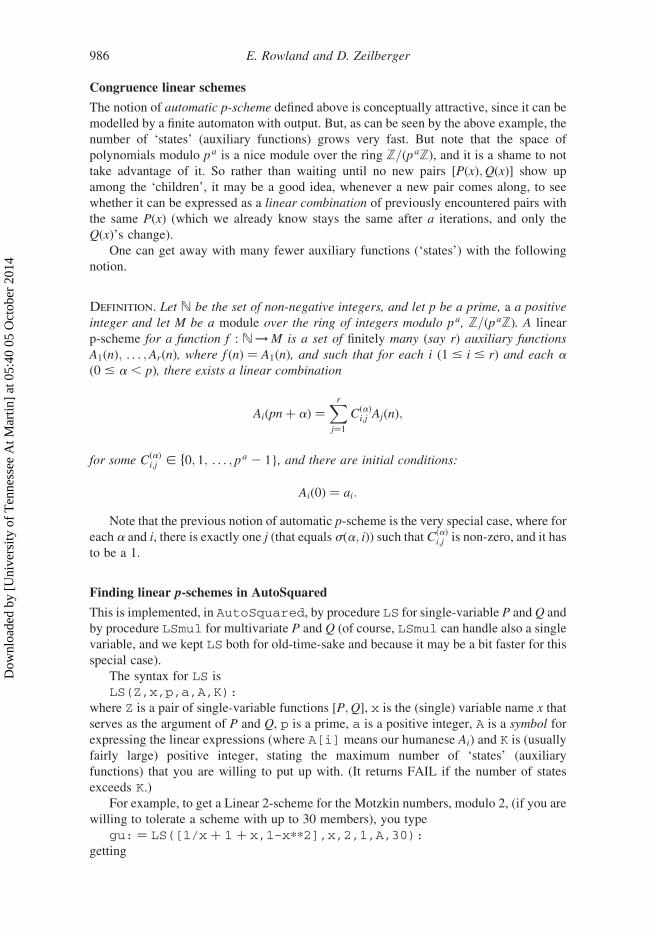
exceeds K.)For example, to get a Linear 2-scheme for the Motzkin numbers, modulo 2, (if you are

willing to tolerate a scheme with up to 30 members), you type

gu: ¼ LS([1/x þ 1 þ x,1-x**2],x,2,1,A,30):getting


Dow

nloa

ded

by [

Uni

vers

ity o

f T

enne

ssee

At M

artin

] at

05:

40 0

5 O

ctob

er 2

014

[[[A[2], A[2]], [A[3], A[4]], [A[3], A[3]], [0, A[2]]], [1, 1,1, 0]] ,which is the same as the automatic 2-scheme, spelled-out above, except it is phrased more

verbosely.

If you type:

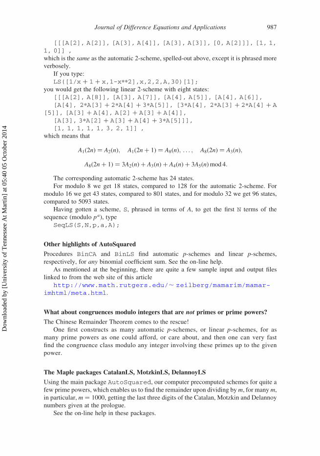
LS([1/x þ 1 þ x,1-x**2],x,2,2,A,30)[1];you would get the following linear 2-scheme with eight states:

[[[A[2], A[8]], [A[3], A[7]], [A[4], A[5]], [A[4], A[6]],[A[4], 2*A[3] þ 2*A[4] þ 3*A[5]], [3*A[4], 2*A[3] þ 2*A[4] þ A

[5]], [A[3] þ A[4], A[2] þ A[3] þ A[4]],[A[3], 3*A[2] þ A[3] þ A[4] þ 3*A[5]]],[1, 1, 1, 1, 1, 3, 2, 1]] ,

which means that

A1ð2nÞ ¼ A2ðnÞ; A1ð2nþ 1Þ ¼ A8ðnÞ; . . . ; A8ð2nÞ ¼ A3ðnÞ;A8ð2nþ 1Þ ¼ 3A2ðnÞ þ A3ðnÞ þ A4ðnÞ þ 3A5ðnÞmod 4:

The corresponding automatic 2-scheme has 24 states.

For modulo 8 we get 18 states, compared to 128 for the automatic 2-scheme. For

modulo 16 we get 43 states, compared to 801 states, and for modulo 32 we get 96 states,

compared to 5093 states.

Having gotten a scheme, S, phrased in terms of A, to get the first N terms of the

sequence (modulo pa), type

SeqLS(S,N,p,a,A);

Other highlights of AutoSquared

Procedures BinCA and BinLS find automatic p-schemes and linear p-schemes,

respectively, for any binomial coefficient sum. See the on-line help.

As mentioned at the beginning, there are quite a few sample input and output files

linked to from the web site of this article

http://www.math.rutgers.edu/, zeilberg/mamarim/mamar-imhtml/meta.html.

What about congruences modulo integers that are not primes or prime powers?

The Chinese Remainder Theorem comes to the rescue!

One first constructs as many automatic p-schemes, or linear p-schemes, for as

many prime powers as one could afford, or care about, and then one can very fast

find the congruence class modulo any integer involving these primes up to the given

power.

The Maple packages CatalanLS, MotzkinLS, DelannoyLS

Using the main package AutoSquared, our computer precomputed schemes for quite a

few prime powers, which enables us to find the remainder upon dividing bym, for manym,

in particular, m ¼ 1000, getting the last three digits of the Catalan, Motzkin and Delannoy

numbers given at the prologue.

See the on-line help in these packages.


Dow

nloa

ded

by [

Uni

vers

ity o

f T

enne

ssee

At M

artin

] at

05:

40 0

5 O

ctob

er 2

014




Disclaimer

Both the automatic p-schemes and the linear p-schemes that our Maple package outputs

are not guaranteed to be minimal. Of course the size does not change the fact that they run

in logarithmic time in the input, but the ‘implied constants’ in the Oðlog nÞ algorithms are

most probably not best possible.

Conclusion

The present project is yet another case study in teaching computers to do research all by

themselves, once they were taught (programmed) the human tricks. Once the computer

mastered them, it can reproduce, in a few seconds, all the previous results accomplished by

humans, and go on to output much deeper results, which no human, by himself, or herself,

would be able to do, hence getting much deeper results. So the fact that the last three

decimal digits ofMgoogol are 187 may not be as interesting as Fermat’s last theorem, but is,

in some sense, much deeper!

Acknowledgements

The second author (DZ) was supported in part by a grant from the National Science Foundation ofthe USA. The authors thank Shalosh B. Ekhad for its many diligent and tedious computations andproofs!

Note

1. Email: [email protected]

References

[1] M. Kauers, C. Krattenthaler, and T.W. Muller, A method for determining the mod-2k behaviourof recursive sequences, with applications to subgroup counting, Electron. J. Combin. 18(2)(2012), Article P37. Available at http://arxiv.org/abs/1107.2015

[2] C. Krattenthaler and T.W. Muller, A method for determining the mod-3k behaviour of recursivesequences, preprint. Available at http://arxiv.org/abs/1308.2856

[3] C. Krattenthaler and T.W. Muller, A Riccati differential equation and free subgroup numbers forlifts of PSL2(Z) modulo powers of primes, J. Combin. Theory Ser. A 120 (2013), pp. 2039–2063.Available at http://arxiv.org/abs/1211.2947

[4] G.E. Revesz, Introduction to Formal Languages, Dover, New York, 1991. [Originally publishedby McGraw-Hill, 1983].

[5] E. Rowland and R. Yassawi, Automatic congruences for diagonals of rational functions.Available at http://arxiv.org/abs/1310.8635


Dow

nloa

ded

by [

Uni

vers

ity o

f T

enne

ssee

At M

artin

] at

05:

40 0

5 O

ctob

er 2

014



http://arxiv.org/abs/1107.2015




Documents

A case study in meta-automation: automatic generation of congruence automata for combinatorial sequences