A Carleman type estimate for the Mindlin-Timoshenko plate

Clemson UniversityTigerPrints

All Theses Theses

5-2017

A Carleman type estimate for the Mindlin-Timoshenko plate modelJason A. KurzClemson University, [email protected]

Follow this and additional works at: https://tigerprints.clemson.edu/all_theses

This Thesis is brought to you for free and open access by the Theses at TigerPrints. It has been accepted for inclusion in All Theses by an authorizedadministrator of TigerPrints. For more information, please contact [email protected].

Recommended CitationKurz, Jason A., "A Carleman type estimate for the Mindlin-Timoshenko plate model" (2017). All Theses. 2647.https://tigerprints.clemson.edu/all_theses/2647

https://tigerprints.clemson.edu?utm_source=tigerprints.clemson.edu%2Fall_theses%2F2647&utm_medium=PDF&utm_campaign=PDFCoverPages

https://tigerprints.clemson.edu/all_theses?utm_source=tigerprints.clemson.edu%2Fall_theses%2F2647&utm_medium=PDF&utm_campaign=PDFCoverPages

https://tigerprints.clemson.edu/theses?utm_source=tigerprints.clemson.edu%2Fall_theses%2F2647&utm_medium=PDF&utm_campaign=PDFCoverPages

https://tigerprints.clemson.edu/all_theses?utm_source=tigerprints.clemson.edu%2Fall_theses%2F2647&utm_medium=PDF&utm_campaign=PDFCoverPages

https://tigerprints.clemson.edu/all_theses/2647?utm_source=tigerprints.clemson.edu%2Fall_theses%2F2647&utm_medium=PDF&utm_campaign=PDFCoverPages

mailto:[email protected]

A Carleman type estimate for the Mindlin-TimoshenkoPlate Model

A Dissertation

Presented to

the Graduate School of

Clemson University

In Partial Fulfillment

of the Requirements for the Degree

Master of Science

Mathematics

by

Jason A. Kurz

May 2017

Accepted by:

Dr. Shitao Liu, Committee Chair

Dr. Mishko Mitkovski

Dr. Jeong-Rock Yoon

Abstract

This thesis focuses on results concerning providing a Carleman type estimate for the Mindlin-

Timoshenko plate equations. The main approach is to provide an estimate for each of the three

equations in the model then present these estimates in totality as a singular Carleman estimate

for the entire model. The initial equation in the model is a simple two dimensional hyperbolic

partial differential equation known as the wave equation. Prior research has been done for this

type of equation and will be applied to provide the Carleman estimate for the first equation in the

model. The estimate for the second and third equations will be derived by first establishing a point-

wise inequality for the principal part of the equation multiplied by an exponential weight. After

establishing a suitable pseudo-convex function for the exponential weight factor, specifications will

be applied to the established point-wise estimates which will lead to the Carleman type estimates

and their corresponding integral inequalities.

ii

Table of Contents

Title Page . . . . . . . . . . . . . . . . . . . . . . . . . . . . . . . . . . . . . . . . . . . . i

Abstract . . . . . . . . . . . . . . . . . . . . . . . . . . . . . . . . . . . . . . . . . . . . . ii

1 Introduction . . . . . . . . . . . . . . . . . . . . . . . . . . . . . . . . . . . . . . . . . 11.1 Background . . . . . . . . . . . . . . . . . . . . . . . . . . . . . . . . . . . . . . . . . 11.2 The Model . . . . . . . . . . . . . . . . . . . . . . . . . . . . . . . . . . . . . . . . . 21.3 Carleman Estimate for Wave Equation in 2D . . . . . . . . . . . . . . . . . . . . . . 31.4 Some Literature on Carleman estimates . . . . . . . . . . . . . . . . . . . . . . . . . 4

2 A Fundamental Lemma . . . . . . . . . . . . . . . . . . . . . . . . . . . . . . . . . . 72.1 Lemma . . . . . . . . . . . . . . . . . . . . . . . . . . . . . . . . . . . . . . . . . . . 72.2 Statement of Lemma as applied to equation (1.4) . . . . . . . . . . . . . . . . . . . . 18

3 Carleman Estimate . . . . . . . . . . . . . . . . . . . . . . . . . . . . . . . . . . . . . 203.1 Basic Assumptions . . . . . . . . . . . . . . . . . . . . . . . . . . . . . . . . . . . . . 203.2 A resulting pointwise inequality . . . . . . . . . . . . . . . . . . . . . . . . . . . . . . 233.3 Carleman estimate for equations (1.3) and (1.4) . . . . . . . . . . . . . . . . . . . . . 283.4 Carleman estimate for the Mindlin-Timoshenko model . . . . . . . . . . . . . . . . . 33

4 Conclusions and Discussion . . . . . . . . . . . . . . . . . . . . . . . . . . . . . . . . 354.1 Purpose of the Estimate . . . . . . . . . . . . . . . . . . . . . . . . . . . . . . . . . . 364.2 Recommendations for Further Research . . . . . . . . . . . . . . . . . . . . . . . . . 36

References . . . . . . . . . . . . . . . . . . . . . . . . . . . . . . . . . . . . . . . . . . . . 37

iii

Chapter 1

Introduction

1.1 Background

The motivations behind the study of the model explored in the thesis has developed from the

classical Euler-Bernoulli beam theory as well as Kirchoff-Love plate models [2, 10]. In more recent

years, models which account for shear deformations have been of more interest and the models in

classical beam theory are limited in their description of plates or beams experiencing high-frequency

vibrations [2, 10]. A model accounting for the transverse shear deformation occurring to the plate

involving two shear angles was considered by Reissner [2, 11]. Reissner’s model possessed several

deviations from classical plate theory, including allowing for a change in the thickness of the plate due

to stresses [11]. These were also changes from Timoshenko’s earlier proposed model, which considered

the displacement of a beam taking into account a single shear angle of its filament [2, 10, 15]. A

later model was proposed by Mindlin, independent of Reissner, that also considered two shear

angles, and has been foundational in the development of modern plate theory [2, 9, 10]. The

Mindlin-Timoshenko model considered for this present paper was considered in Lagnese [4] with

explorations of the systems stability and well-posedness researched by Pei et al. [10], Jorge Silva et

al. [13], Grobbelaar-Van Dalsen [2], and Fernandez Sare [12]. The Mindlin-Timoshenko model is the

one of interest for the purposes of the research presented in this paper with the goal of presenting a

Carleman type estimate for the model.

1

1.2 The Model

This paper will be studying the Mindlin-Timoshenko plate model in the two dimensional

case given by

ρhwtt −K∆w −K(φx + ψy) = 0, in Ω× [0, T ]

ρh3

12 ψtt −D(ψxx + 1−µ

2 ψyy)−D

(1+µ

2 φxy)

+K(ψ + wx) = 0, in Ω× [0, T ]

ρh3

12 φtt −D(φyy + 1−µ

2 φxx)−D

(1+µ

2 ψxy)

+K(φ+ wy) = 0 in Ω× [0, T ]

(1.1)

with initial conditions (w(x, y, 0), ψ(x, y, 0), φ(x, y, 0)) = (w0, ψ0, ψ0) ∈ (H10 (Ω))3

(wt(x, y, 0), ψt(x, y, 0), φt(x, y, 0)) = (w1, ψ1, ψ1) ∈ (L2(Ω))3

and boundary conditions

w = ψ = φ = 0 on ∂Ω× [0, T ]

where Ω ⊂ R2 is an open bounded domain and ρ, h,D and K are positive constants representing the

mass per unit surface area, thickness of the plate, flexural rigidity and shear modulus respectively [12,

10, 13]. Notice w is displacement of the plate from the central plane in the normal direction to the

mid-surface plane, while φ and ψ are the angles of shear deformation [12]. The constant µ is referred

to as Poisson’s ratio constrained by 0 < µ < 12 in physical situations [12, 10, 13]. The term 1−µ

2

will play a central role in parts of this paper and will be denoted as a for the purposes of easing the

notation. For the purposes of the results presented, the simplified model given by

wtt −∆w − (φx + ψy) = 0, in Ω× [0, T ] (1.2)

ψtt −(ψxx +

1− µ2

ψyy

)− 1 + µ

2φxy + (ψ + wx) = 0, in Ω× [0, T ] (1.3)

φtt −(

1− µ2

φxx + φyy

)− 1 + µ

2ψxy + (φ+ wy) = 0, in Ω× [0, T ] (1.4)

will be used for this paper.

2

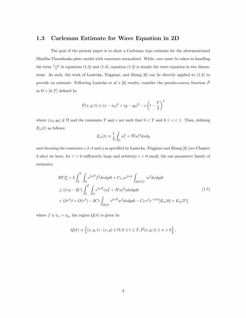
1.3 Carleman Estimate for Wave Equation in 2D

The goal of the present paper is to show a Carleman type estimate for the aforementioned

Mindlin-Timoshenko plate model with constants normalized. While, care must be taken in handling

the term 1−µ2 in equations (1.3) and (1.4), equation (1.2) is simply the wave equation in two dimen-

sions. As such, the work of Lasiecka, Triggiani, and Zhang [6] can be directly applied to (1.2) to

provide an estimate. Following Lasiecka et al.’s [6] results, consider the pseudo-convex function P

in Ω× [0, T ] defined by

P (x, y, t) ≡ (x− x0)2 + (y − y0)2 − c(t− T

2

)2

where (x0, y0) /∈ Ω and the constants T and c are such that 0 < T and 0 < c < 1. Then, defining

Ew(t) as follows:

Ew(t) ≡ 1

2

∫Ω

w2t + |∇w|2dxdy

and choosing the constants c, σ, δ and ρ as specified by Lasiecka, Triggiani and Zhang [6] (see Chapter

3 also) we have, for τ > 0 sufficiently large and arbitrary ε > 0 small, the one parameter family of

estimates

BT |wΣ + 2

∫ T

0

∫Ω

e2τP f2dxdydt+ C1,T e2τσ

∫[Q(σ)]c

w2dxdydt

≥ (ετρ− 2C)

∫ T

0

∫Ω

e2τP (w2t + |∇w|2)dxdydt

+ (2τ3β +O(τ2)− 2C)

∫Q(σ)

e2τPw2dxdydt− CT τ3e−2τδ[Ew(0) + Ew(T )]

(1.5)

where f ≡ ψx + φy, the region Q(σ) is given by

Q(σ) ≡

(x, y, t) : (x, y) ∈ Ω, 0 ≤ t ≤ T, P (x, y, t) ≥ σ > 0,

3

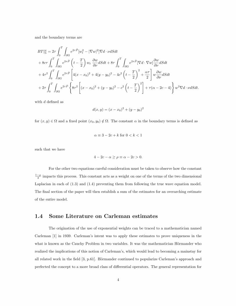
and the boundary terms are

BT |wΣ = 2τ

∫ T

0

∫∂Ω

e2τP [w2t − |∇w|2]∇d · νdSdt

+ 8cτ

∫ T

0

∫∂Ω

e2τP

(t− T

2

)wt

∂w

∂νdSdt+ 8τ

∫ T

0

∫∂Ω

e2τP [∇d · ∇w]∂w

∂νdSdt

+ 4τ2

∫ T

0

∫∂Ω

e2τP

[4(x− x0)2 + 4(y − y0)2 − 4c2

(t− T

2

)2

+ατ

2

]w∂w

∂νdSdt

+ 2τ

∫ T

0

∫∂Ω

e2τP

8τ2

[(x− x0)2 + (y − y0)2 − c2

(t− T

2

)2]

+ τ(α− 2c− 4)

w2∇d · νdSdt.

with d defined as

d(x, y) = (x− x0)2 + (y − y0)2

for (x, y) ∈ Ω and a fixed point (x0, y0) /∈ Ω. The constant α in the boundary terms is defined as

α ≡ 3− 2c+ k for 0 < k < 1

such that we have

4− 2c− α ≥ ρ ≡ α− 2c > 0.

For the other two equations careful consideration must be taken to observe how the constant

1−µ2 impacts this process. This constant acts as a weight on one of the terms of the two dimensional

Laplacian in each of (1.3) and (1.4) preventing them from following the true wave equation model.

The final section of the paper will then establish a sum of the estimates for an overarching estimate

of the entire model.

1.4 Some Literature on Carleman estimates

The origination of the use of exponential weights can be traced to a mathematician named

Carleman [1] in 1939. Carleman’s intent was to apply these estimates to prove uniqueness in the

what is known as the Cauchy Problem in two variables. It was the mathematician Hormander who

realized the implications of this notion of Carleman’s, which would lead to becoming a mainstay for

all related work in the field [3, p.61]. Hormander continued to popularize Carleman’s approach and

perfected the concept to a more broad class of differential operators. The general representation for

4

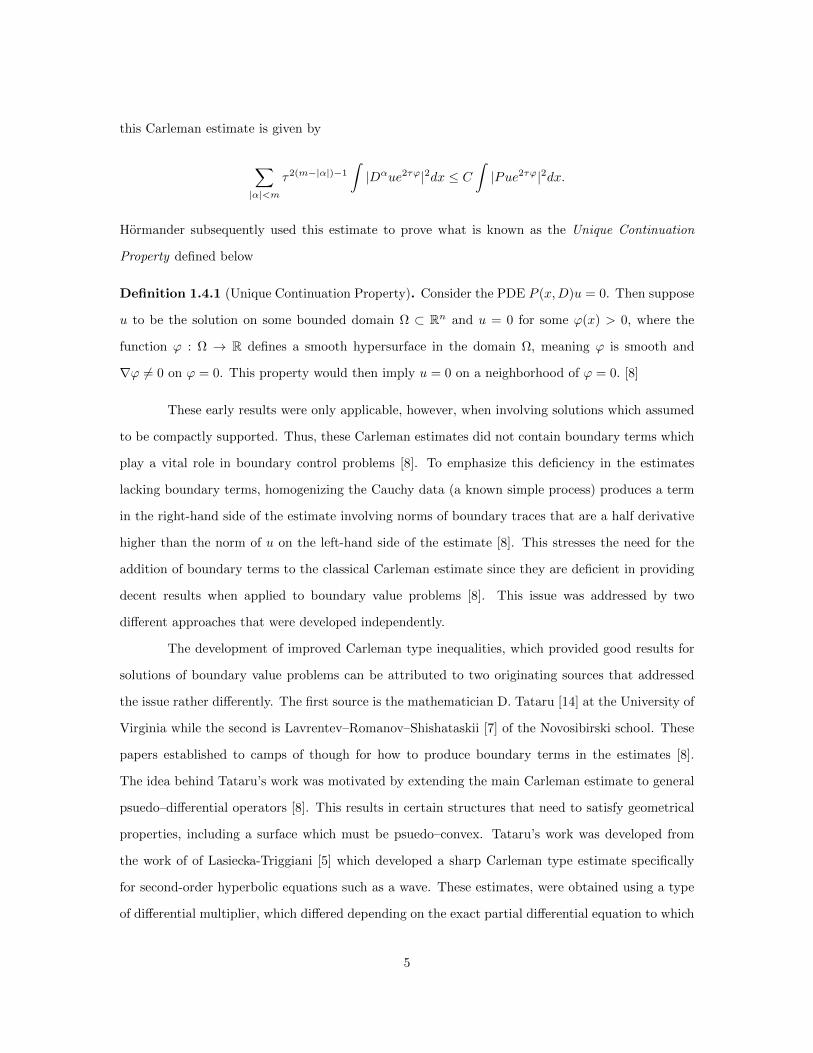
this Carleman estimate is given by

∑|α|<m

τ2(m−|α|)−1

∫|Dαue2τϕ|2dx ≤ C

∫|Pue2τϕ|2dx.

Hormander subsequently used this estimate to prove what is known as the Unique Continuation

Property defined below

Definition 1.4.1 (Unique Continuation Property). Consider the PDE P (x,D)u = 0. Then suppose

u to be the solution on some bounded domain Ω ⊂ Rn and u = 0 for some ϕ(x) > 0, where the

function ϕ : Ω → R defines a smooth hypersurface in the domain Ω, meaning ϕ is smooth and

∇ϕ 6= 0 on ϕ = 0. This property would then imply u = 0 on a neighborhood of ϕ = 0. [8]

These early results were only applicable, however, when involving solutions which assumed

to be compactly supported. Thus, these Carleman estimates did not contain boundary terms which

play a vital role in boundary control problems [8]. To emphasize this deficiency in the estimates

lacking boundary terms, homogenizing the Cauchy data (a known simple process) produces a term

in the right-hand side of the estimate involving norms of boundary traces that are a half derivative

higher than the norm of u on the left-hand side of the estimate [8]. This stresses the need for the

addition of boundary terms to the classical Carleman estimate since they are deficient in providing

decent results when applied to boundary value problems [8]. This issue was addressed by two

different approaches that were developed independently.

The development of improved Carleman type inequalities, which provided good results for

solutions of boundary value problems can be attributed to two originating sources that addressed

the issue rather differently. The first source is the mathematician D. Tataru [14] at the University of

Virginia while the second is Lavrentev–Romanov–Shishataskii [7] of the Novosibirski school. These

papers established to camps of though for how to produce boundary terms in the estimates [8].

The idea behind Tataru’s work was motivated by extending the main Carleman estimate to general

psuedo–differential operators [8]. This results in certain structures that need to satisfy geometrical

properties, including a surface which must be psuedo–convex. Tataru’s work was developed from

the work of of Lasiecka-Triggiani [5] which developed a sharp Carleman type estimate specifically

for second-order hyperbolic equations such as a wave. These estimates, were obtained using a type

of differential multiplier, which differed depending on the exact partial differential equation to which

5

it was applied [8]. In contrast, Lavrentev–Romanov–Shishaskii [7] approached the problem of pro-

ducing boundary terms in the estimate via a format which was much more computationally focused.

Their method was to establish an initial point–wise Carleman estimate with the resulting integral

form of this estimate [8]. This was the inspiration behind the subsequent work of Lasiecka-Triggiani-

Zhang [6], the primary source for the work in this paper. In their paper, Lasiecka–Triggiani–Zhang [6]

worked via the method produced in the Lavrentev camp by establishing a fundamental initial point–

wise inequality for the general second order hyperbolic equation that was used to produce a a one

parameter family of point–wise Carleman estimates [6].

The Carleman estimates derived for the Mindlin-Timoshenko equations follow the process

established by Lasiecka–Triggiani–Zhang wherein we establish an initial point-wise estimate for

the second and third equations in the system. This estimate will then, via careful selection of

an appropriate pseudo–convex function and other specifications, will ultimately yield point–wise

Carleman estimates, and followed by the corresponding integral inequalities. The final estimate is

expressed in terms of these point–wise integral inequalities.

The organization for the main result of this thesis is as follows: In Chapter 2 we prove the

main point–wise estimates for the equations of two shear angles in the model. In Chapter 3 we will

derive the Carleman estimates by introducing a suitable pseudo-convex function that is needed for

the special structure of the equations (1.3) and (1.4).

6

Chapter 2

A Fundamental Lemma

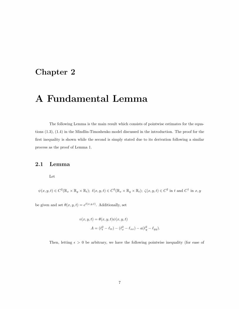
The following Lemma is the main result which consists of pointwise estimates for the equa-

tions (1.3), (1.4) in the Mindlin-Timoshenko model discussed in the introduction. The proof for the

first inequality is shown while the second is simply stated due to its derivation following a similar

process as the proof of Lemma 1.

2.1 Lemma

Let

ψ(x, y, t) ∈ C2(Rx × Ry × Rt); `(x, y, t) ∈ C3(Rx × Ry × Rt); ζ(x, y, t) ∈ C2 in t and C1 in x, y

be given and set θ(x, y, t) = e`(x,y,t). Additionally, set

v(x, y, t) = θ(x, y, t)ψ(x, y, t)

A = (`2t − `tt)− (`2x − `xx)− a(`2y − `yy).

Then, letting ε > 0 be arbitrary, we have the following pointwise inequality (for ease of

7

computation, we use the substitution a = 1−µ2 throughout the statement and proof of the lemma)

θ2[ψtt − (ψxx + aψyy)]2 − ∂

∂t

θ2[−2`t(ψ

2t + ψ2

x + aψ2y) + 4ψt(`xψx + a`yψy) + 2(2`2x + 2a`2y − 2`2t + ζ)ψψt

+(2`t(`2x + a`2y)− 2`3t − 2A`t − ζt)ψ2]

+ 2

∂

∂x

θ2[2ψx(`xψx + aψy`y − ψt`t)− `x(ψ2

x + aψ2y − ψ2

t )

+2

(`2x + a`2y − `2t +

ζ

2

)ψxψ + `x(`2x + a`2y − `2t −A)ψ2]

+ 2a

∂

∂y

θ2[2ψy(`xψx + aψy`y)− `y(ψ2

x + aψ2y)− 2`tψyψt + `yψ

2t

+2

(`2x + a`2y − `2t +

ζ

2

)ψyψ + `y(`2x + a`2y − `2t −A)ψ2]

≥ −8vt(`xtvx + a`ytvy) + 2(`xx + a`yy + `tt − ζ)v2

t

+ 2(ζ − ε

2− `xx − a`yy + `tt)(v

2x + av2

y) + 4(`xxv2x + 2a`xyvxvy + a2`yyv

2y)

2Aζ − 2

[∂

∂x((A+ ζ)`x) + a

∂

∂y((A+ ζ)`y)− ∂

∂t((A+ ζ)`t)

]− 1

ε(ζ2x + aζ2

y ) + ζtt

v2

(2.1)

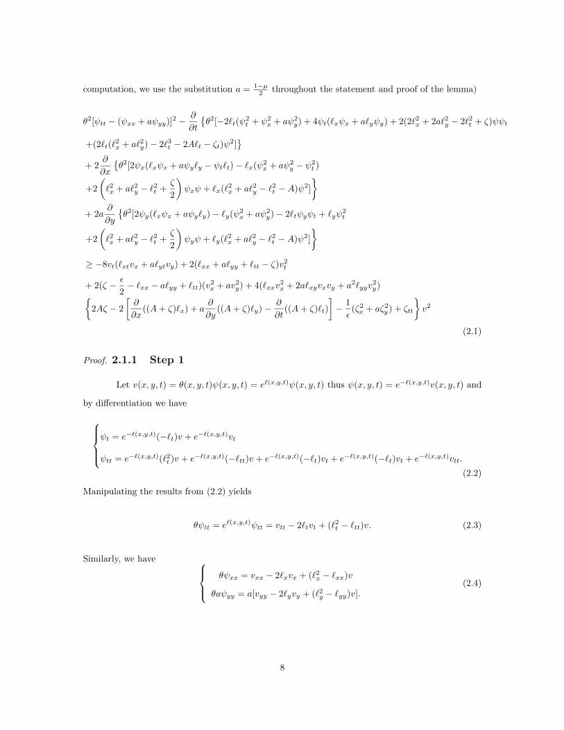
Proof. 2.1.1 Step 1

Let v(x, y, t) = θ(x, y, t)ψ(x, y, t) = e`(x,y,t)ψ(x, y, t) thus ψ(x, y, t) = e−`(x,y,t)v(x, y, t) and

by differentiation we have

ψt = e−`(x,y,t)(−`t)v + e−`(x,y,t)vt

ψtt = e−`(x,y,t)(`2t )v + e−`(x,y,t)(−`tt)v + e−`(x,y,t)(−`t)vt + e−`(x,y,t)(−`t)vt + e−`(x,y,t)vtt.

(2.2)

Manipulating the results from (2.2) yields

θψtt = e`(x,y,t)ψtt = vtt − 2`tvt + (`2t − `tt)v. (2.3)

Similarly, we have θψxx = vxx − 2`xvx + (`2x − `xx)v

θaψyy = a[vyy − 2`yvy + (`2y − `yy)v].(2.4)

8

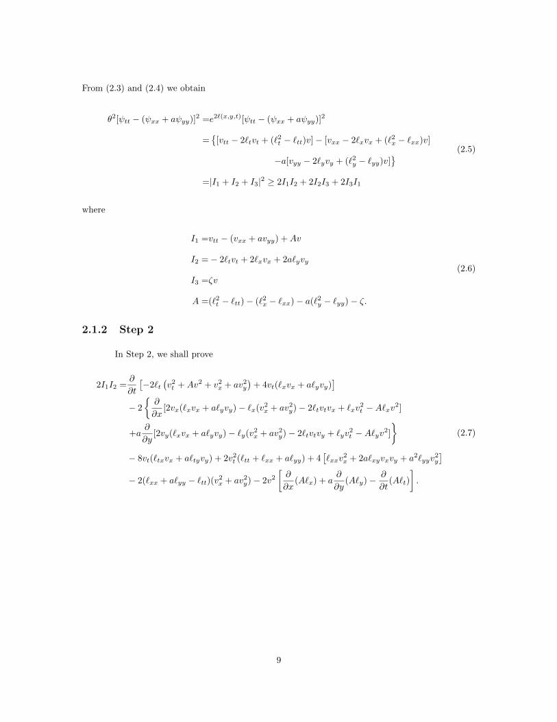
From (2.3) and (2.4) we obtain

θ2[ψtt − (ψxx + aψyy)]2 =e2`(x,y,t)[ψtt − (ψxx + aψyy)]2

=

[vtt − 2`tvt + (`2t − `tt)v]− [vxx − 2`xvx + (`2x − `xx)v]

−a[vyy − 2`yvy + (`2y − `yy)v]

=|I1 + I2 + I3|2 ≥ 2I1I2 + 2I2I3 + 2I3I1

(2.5)

where

I1 =vtt − (vxx + avyy) +Av

I2 =− 2`tvt + 2`xvx + 2a`yvy

I3 =ζv

A =(`2t − `tt)− (`2x − `xx)− a(`2y − `yy)− ζ.

(2.6)

2.1.2 Step 2

In Step 2, we shall prove

2I1I2 =∂

∂t

[−2`t

(v2t +Av2 + v2

x + av2y

)+ 4vt(`xvx + a`yvy)

]− 2

∂

∂x[2vx(`xvx + a`yvy)− `x(v2

x + av2y)− 2`tvtvx + `xv

2t −A`xv2]

+a∂

∂y[2vy(`xvx + a`yvy)− `y(v2

x + av2y)− 2`tvtvy + `yv

2t −A`yv2]

− 8vt(`txvx + a`tyvy) + 2v2

t (`tt + `xx + a`yy) + 4[`xxv

2x + 2a`xyvxvy + a2`yyv

2y

]− 2(`xx + a`yy − `tt)(v2

x + av2y)− 2v2

[∂

∂x(A`x) + a

∂

∂y(A`y)− ∂

∂t(A`t)

].

(2.7)

9

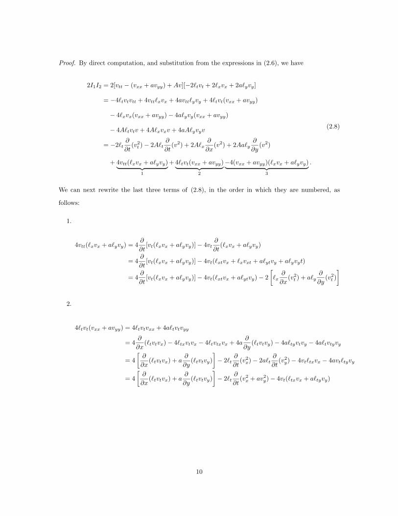
Proof. By direct computation, and substitution from the expressions in (2.6), we have

2I1I2 = 2[vtt − (vxx + avyy) +Av][−2`tvt + 2`xvx + 2a`yvy]

= −4`tvtvtt + 4vtt`xvx + 4avtt`yvy + 4`tvt(vxx + avyy)

− 4`xvx(vxx + avyy)− 4a`yvy(vxx + avyy)

− 4A`tvtv + 4A`xvxv + 4aA`yvyv

= −2`t∂

∂t(v2t )− 2A`t

∂

∂t(v2) + 2A`x

∂

∂x(v2) + 2Aa`y

∂

∂y(v2)

+ 4vtt(`xvx + a`yvy)︸︷︷︸1

+ 4`tvt(vxx + avyy)︸︷︷︸2

−4(vxx + avyy)(`xvx + a`yvy)︸︷︷︸3

.

(2.8)

We can next rewrite the last three terms of (2.8), in the order in which they are numbered, as

follows:

1.

4vtt(`xvx + a`yvy) = 4∂

∂t[vt(`xvx + a`yvy)]− 4vt

∂

∂t(`xvx + a`yvy)

= 4∂

∂t[vt(`xvx + a`yvy)]− 4vt(`xtvx + `xvxt + a`ytvy + a`yvyt)

= 4∂

∂t[vt(`xvx + a`yvy)]− 4vt(`xtvx + a`ytvy)− 2

[`x

∂

∂x(v2t ) + a`y

∂

∂y(v2t )

]

2.

4`tvt(vxx + avyy) = 4`tvtvxx + 4a`tvtvyy

= 4∂

∂x(`tvtvx)− 4`txvtvx − 4`tvtxvx + 4a

∂

∂y(`tvtvy)− 4a`tyvtvy − 4a`tvtyvy

= 4

[∂

∂x(`tvtvx) + a

∂

∂y(`tvtvy)

]− 2`t

∂

∂t(v2x)− 2a`t

∂

∂t(v2y)− 4vt`txvx − 4avt`tyvy

= 4

[∂

∂x(`tvtvx) + a

∂

∂y(`tvtvy)

]− 2`t

∂

∂t(v2x + av2

y)− 4vt(`txvx + a`tyvy)

10

3.

−4(vxx + avyy)(`xvx + a`yvy)

= −4vxx`xvx − 4avxx`yvy − 4avyy`xvx − 4a2vyy`yvy

= −4∂

∂x(v2x`x) + 4v2

x`xx + 4vx`xvxx − 4a∂

∂x(vx`yvy) + 4avx`yxvy + 4avx`yvyx

− 4a2 ∂

∂y(v2y`y) + 4a2v2

y`yy + 4a2vy`yvyy − 4a∂

∂y(vy`xvx) + 4avy`xyvx + 4avy`xvxy

= −4

[∂

∂x(v2x`x + avx`yvy) +

∂

∂y(avy`xvx + a2v2

y`y)

]+ 4[`xxv

2x + a`yxvxvy + a`xyvxvy + a2`yyv

2y]

+ 2

[`x

∂

∂x(v2x) + a`y

∂

∂y(v2y) + a`x

∂

∂x(v2y) + a2`y

∂

∂y(v2y)

]

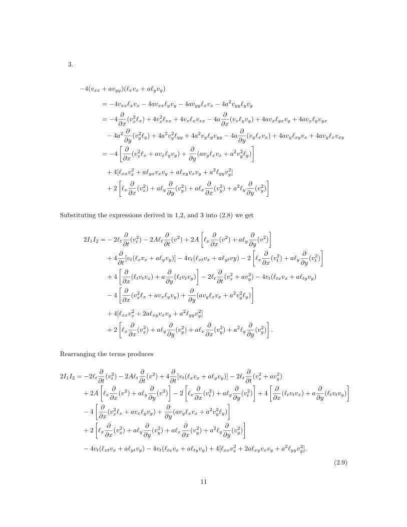
Substituting the expressions derived in 1,2, and 3 into (2.8) we get

2I1I2 =− 2`t∂

∂t(v2t )− 2A`t

∂

∂t(v2) + 2A

[`x

∂

∂x(v2) + a`y

∂

∂y(v2)

]+ 4

∂

∂t[vt(`xvx + a`yvy)]− 4vt(`xtvx + a`ytvy)− 2

[`x

∂

∂x(v2t ) + a`y

∂

∂y(v2t )

]+ 4

[∂

∂x(`tvtvx) + a

∂

∂y(`tvtvy)

]− 2`t

∂

∂t(v2x + av2

y)− 4vt(`txvx + a`tyvy)

− 4

[∂


∂

∂y(avy`xvx + a2v2

y`y)

]+ 4[`xxv


2y]

+ 2

[`x

∂

∂x(v2x) + a`y

∂

∂y(v2y) + a`x

∂

∂x(v2y) + a2`y

∂

∂y(v2y)

].

Rearranging the terms produces

2I1I2 = −2`t∂

∂t(v2t )− 2A`t

∂

∂t(v2) + 4

∂

∂t[vt(`xvx + a`yvy)]− 2`t

∂

∂t(v2x + av2

y)

+ 2A

[`x

∂

∂x(v2) + a`y

∂

∂y(v2)

]− 2

[`x

∂

∂x(v2t ) + a`y

∂

∂y(v2t )

]+ 4

[∂

∂x(`tvtvx) + a

∂

∂y(`tvtvy)

]− 4

[∂


∂

∂y(avy`xvx + a2v2

y`y)

]+ 2

[`x

∂

∂x(v2x) + a`y

∂

∂y(v2y) + a`x

∂

∂x(v2y) + a2`y

∂

∂y(v2y)

]− 4vt(`xtvx + a`ytvy)− 4vt(`txvx + a`tyvy) + 4[`xxv


2y].

(2.9)

11

Grouping the ∂∂t terms in (2.9) yields

∂

∂t

[−2`tv

2t − 2A`tv

2 − 2`t(v2x + av2

y) + 4vt(`xvx + a`yvy)]

+ 2`ttv2t + 2v2 ∂

∂t(A`t) + 2`tt(v

2x + av2

y).

(2.10)

Grouping the ∂∂x and ∂

∂y terms we have

∂

∂x[2A`xv

2 − 2`xv2t + 4`tvtvx − 4vx(`xvx + a`yvy) + 2`x(v2

x + av2y)]

+ a∂

∂y[2A`yv

2 − 2`yv2t + 4`tvtvy − 4vy(`xvx + a`yvy) + 2`y(v2

x + av2y)]

− 2v2

[∂

∂x(A`x) + a

∂

∂y(A`y)

]+ 2v2

t (`xx + a`yy)− 2(`xx + a`yy)(v2x + av2

y).

(2.11)

Finally, substituting (2.10) and (2.11) into (2.9) and rearranging the terms gives the result in (2.7).

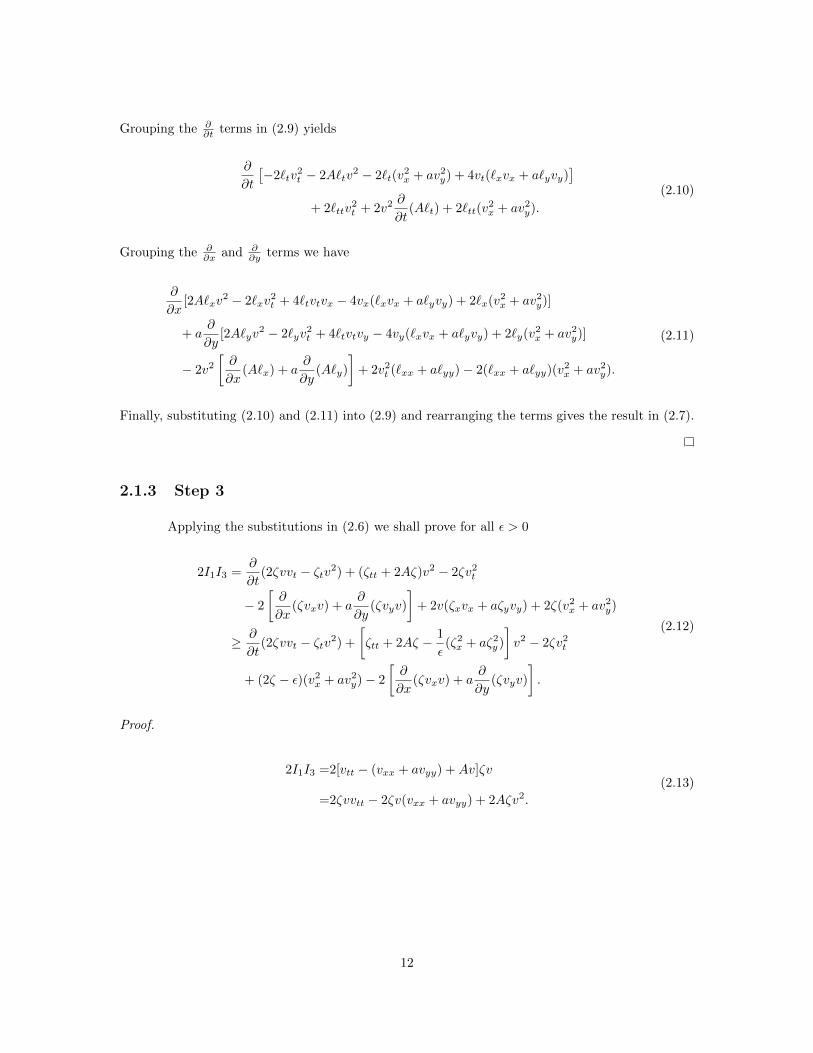
2.1.3 Step 3

Applying the substitutions in (2.6) we shall prove for all ε > 0

2I1I3 =∂

∂t(2ζvvt − ζtv2) + (ζtt + 2Aζ)v2 − 2ζv2

t

− 2

[∂

∂x(ζvxv) + a

∂

∂y(ζvyv)

]+ 2v(ζxvx + aζyvy) + 2ζ(v2

x + av2y)

≥ ∂

∂t(2ζvvt − ζtv2) +

[ζtt + 2Aζ − 1

ε(ζ2x + aζ2

y )

]v2 − 2ζv2

t

+ (2ζ − ε)(v2x + av2

y)− 2

[∂

∂x(ζvxv) + a

∂

∂y(ζvyv)

].

(2.12)

Proof.

2I1I3 =2[vtt − (vxx + avyy) +Av]ζv

=2ζvvtt − 2ζv(vxx + avyy) + 2Aζv2.

(2.13)

12

Where

2ζvvtt = 2∂

∂t(ζvvt)− 2vt

∂

∂t(ζv)

= 2∂

∂t(ζvvt)− 2vtζtv − 2v2

t ζ

= 2∂

∂t(ζvvt)−

∂

∂t(ζtv

2) + ζttv2 − 2v2

t ζ

−2ζv(vxx + avyy) = −2ζvvxx − 2aζvvyy

= −2∂

∂x(ζvvx) + 2vx

∂

∂x(ζv)− 2a

∂

∂y(ζvvy) + 2avy

∂

∂y(ζv)

= −2

[∂

∂x(ζvvx) + a

∂

∂y(ζvvy)

]+ 2ζxvxv + 2aζyvyv + 2ζv2

x + 2aζv2y

= −2

[∂

∂x(ζvvx) + a

∂

∂y(ζvvy)

]+ 2v(ζxvx + aζyvy) + 2ζ(v2

x + av2y).

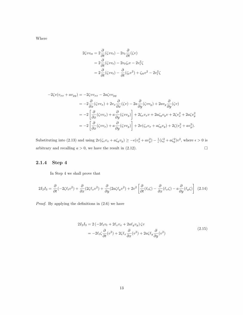
Substituting into (2.13) and using 2v(ζxvx + aζyvy) ≥ −ε(v2x + av2

y)− 1ε (ζ2

x + aζ2y )v2, where ε > 0 is

arbitrary and recalling a > 0, we have the result in (2.12).

2.1.4 Step 4

In Step 4 we shall prove that

2I2I3 =∂

∂t(−2ζ`tv

2) +∂

∂x(2ζ`xv

2) +∂

∂y(2aζ`yv

2) + 2v2

[∂

∂t(`tζ)− ∂

∂x(`xζ)− a ∂

∂y(`yζ)

](2.14)

Proof. By applying the definitions in (2.6) we have

2I2I3 = 2 (−2`tvt + 2`xvx + 2a`yvy) ζv

= −2`tζ∂

∂t(v2) + 2ζ`x

∂

∂x(v2) + 2aζ`y

∂

∂y(v2)

(2.15)

13

Where

−2`tζ∂

∂t(v2) =

∂

∂t(−2`tζv

2) + 2`ttζv2 + 2`tζtv

2

=∂

∂t(−2`tζv

2) + 2v2(`ttζ + `tζt)

=∂

∂t(−2`tζv

2) + 2v2 ∂

∂t(`tζ)

2ζ`x∂

∂x(v2) + 2aζ`y

∂

∂y(v2) =

∂

∂x(2ζ`xv

2)− 2`xxζv2 − 2`xζxv

2

+∂

∂y(2aζ`yv

2)− 2a`yyζv2 − 2a`yζyv

2

=∂

∂x(2ζ`xv

2) +∂

∂y(2aζ`yv

2)− 2v2 ∂

∂x(`xζ)− 2v2 ∂

∂y(a`yζ)

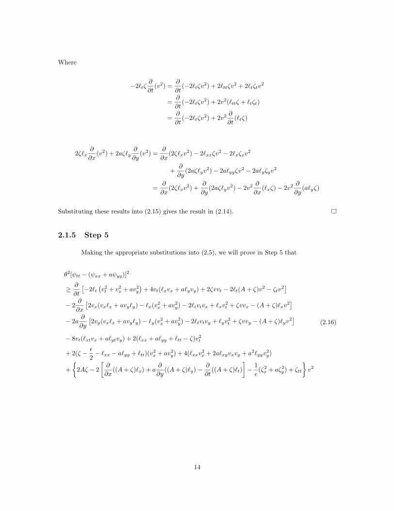
Substituting these results into (2.15) gives the result in (2.14).

2.1.5 Step 5

Making the appropriate substitutions into (2.5), we will prove in Step 5 that

θ2[ψtt − (ψxx + aψyy)]2

≥ ∂

∂t

[−2`t

(v2t + v2

x + av2y

)+ 4vt(`xvx + a`yvy) + 2ζvvt − 2`t(A+ ζ)v2 − ζtv2

]− 2

∂

∂x

[2vx(vx`x + avy`y)− `x(v2


2t + ζvvx − (A+ ζ)`xv

2]

− 2a∂

∂y

[2vy(vx`x + avy`y)− `y(v2


2t + ζvvy − (A+ ζ)`yv

2]

− 8vt(`xtvx + a`ytvy) + 2(`xx + a`yy + `tt − ζ)v2t

+ 2(ζ − ε

2− `xx − a`yy + `tt)(v

2x + av2


2y)

+

2Aζ − 2

[∂

∂x((A+ ζ)`x) + a

∂

∂y((A+ ζ)`y)− ∂

∂t((A+ ζ)`t)

]− 1

ε(ζ2x + aζ2

y ) + ζtt

v2

(2.16)

14

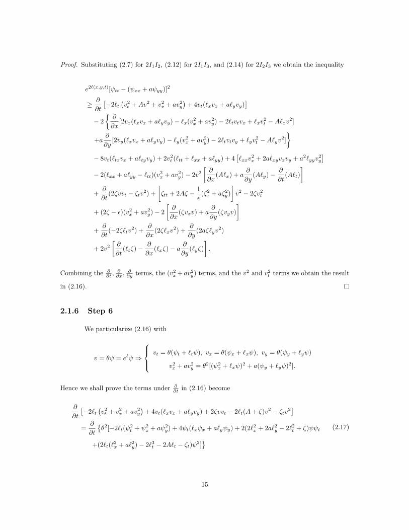
Proof. Substituting (2.7) for 2I1I2, (2.12) for 2I1I3, and (2.14) for 2I2I3 we obtain the inequality

e2`(x,y,t)[ψtt − (ψxx + aψyy)]2

≥ ∂

∂t

[−2`t

(v2t +Av2 + v2

x + av2y

)+ 4vt(`xvx + a`yvy)

]− 2

∂

∂x[2vx(`xvx + a`yvy)− `x(v2


2t −A`xv2]

+a∂

∂y[2vy(`xvx + a`yvy)− `y(v2


2t −A`yv2]

− 8vt(`txvx + a`tyvy) + 2v2

t (`tt + `xx + a`yy) + 4[`xxv


2y

]− 2(`xx + a`yy − `tt)(v2

x + av2y)− 2v2

[∂

∂x(A`x) + a

∂

∂y(A`y)− ∂

∂t(A`t)

]+∂

∂t(2ζvvt − ζtv2) +

[ζtt + 2Aζ − 1

ε(ζ2x + aζ2

y )

]v2 − 2ζv2

t

+ (2ζ − ε)(v2x + av2

y)− 2

[∂

∂x(ζvxv) + a

∂

∂y(ζvyv)

]+∂

∂t(−2ζ`tv

2) +∂

∂x(2ζ`xv

2) +∂

∂y(2aζ`yv

2)

+ 2v2

[∂

∂t(`tζ)− ∂

∂x(`xζ)− a ∂

∂y(`yζ)

].

Combining the ∂∂t ,

∂∂x ,

∂∂y terms, the (v2

x + av2y) terms, and the v2 and v2

t terms we obtain the result

in (2.16).

2.1.6 Step 6

We particularize (2.16) with

v = θψ = e`ψ ⇒

vt = θ(ψt + `tψ), vx = θ(ψx + `xψ), vy = θ(ψy + `yψ)

v2x + av2

y = θ2[(ψ2x + `xψ)2 + a(ψy + `yψ)2].

Hence we shall prove the terms under ∂∂t in (2.16) become

∂

∂t

[−2`t

(v2t + v2

x + av2y


]=

∂

∂t

θ2[−2`t(ψ

2t + ψ2


+(2`t(`2x + a`2y)− 2`3t − 2A`t − ζt)ψ2]

(2.17)

15

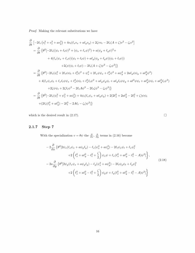
Proof. Making the relevant substitutions we have

∂

∂t

[−2`t

(v2t + v2

x + av2y


]=

∂

∂t

θ2[−2`t((ψt + `tψ)2 + (ψx + `xψ)2) + a(ψy + `yψ)2+

+ 4(`x(ψx + `xψ)(ψt + `tψ) + a`y(ψy + `yψ)(ψt + `tψ))

+2ζψ(ψt + `tψ)− 2`t(A+ ζ)ψ2 − ζtψ2]

=∂

∂t

θ2[−2`t(ψ

2t + 2`tψψt + `2tψ

2 + ψ2x + 2`xψψx + `2xψ

2 + aψ2y + 2a`yψψy + a`2yψ

2)

+ 4(`xψxψt + `x`tψψx + `2xψψt + `2x`tψ2 + a`yψyψt + a`y`tψψy + a`2ψψt + a`2yψψt + a`2y`tψ

2)

+2ζψψt + 2ζ`tψ2 − 2`tAψ

2 − 2`tζψ2 − ζtψ2]

=

∂

∂t

θ2[−2`t(ψ

2t + ψ2


+(2`t(`2x + a`2y)− 2`3t − 2A`t − ζt)ψ2]

which is the desired result in (2.17).

2.1.7 Step 7

With the specialization v = θψ the ∂∂x , ∂

∂y terms in (2.16) become

− 2∂

∂x

θ2[2ψx(`xψx + aψy`y)− `x(ψ2

x + aψ2y)− 2`tψxψt + `xψ

2t

+2

(`2x + a`2y − `2t +

ζ

2

)ψxψ + `x(`2x + a`2y − `2t −A)ψ2]

,

− 2a∂

∂y



2t

+2

(`2x + a`2y − `2t +

ζ

2

)ψyψ + `y(`2x + a`2y − `2t −A)ψ2]

(2.18)

16

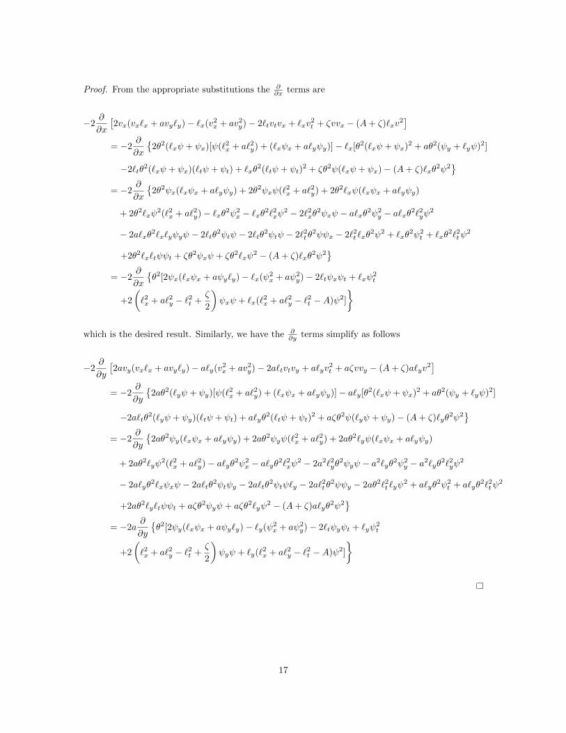
Proof. From the appropriate substitutions the ∂∂x terms are

−2∂

∂x

[2vx(vx`x + avy`y)− `x(v2


2t + ζvvx − (A+ ζ)`xv

2]

= −2∂

∂x

2θ2(`xψ + ψx)[ψ(`2x + a`2y) + (`xψx + a`yψy)]− `x[θ2(`xψ + ψx)2 + aθ2(ψy + `yψ)2]

−2`tθ2(`xψ + ψx)(`tψ + ψt) + `xθ

2(`tψ + ψt)2 + ζθ2ψ(`xψ + ψx)− (A+ ζ)`xθ

2ψ2

= −2∂

∂x

2θ2ψx(`xψx + a`yψy) + 2θ2ψxψ(`2x + a`2y) + 2θ2`xψ(`xψx + a`yψy)

+ 2θ2`xψ2(`2x + a`2y)− `xθ2ψ2

x − `xθ2`2xψ2 − 2`2xθ

2ψxψ − a`xθ2ψ2y − a`xθ2`2yψ

2

− 2a`xθ2`x`yψyψ − 2`tθ

2ψtψ − 2`tθ2ψtψ − 2`2t θ

2ψψx − 2`2t `xθ2ψ2 + `xθ

2ψ2t + `xθ

2`2tψ2

+2θ2`x`tψψt + ζθ2ψxψ + ζθ2`xψ2 − (A+ ζ)`xθ

2ψ2

= −2∂

∂x



2t

+2

(`2x + a`2y − `2t +

ζ

2

)ψxψ + `x(`2x + a`2y − `2t −A)ψ2]

which is the desired result. Similarly, we have the ∂∂y terms simplify as follows

−2∂

∂y

[2avy(vx`x + avy`y)− a`y(v2

x + av2y)− 2a`tvtvy + a`yv

2t + aζvvy − (A+ ζ)a`yv

2]

= −2∂

∂y

2aθ2(`yψ + ψy)[ψ(`2x + a`2y) + (`xψx + a`yψy)]− a`y[θ2(`xψ + ψx)2 + aθ2(ψy + `yψ)2]

−2a`tθ2(`yψ + ψy)(`tψ + ψt) + a`yθ

2(`tψ + ψt)2 + aζθ2ψ(`yψ + ψy)− (A+ ζ)`yθ

2ψ2

= −2∂

∂y

2aθ2ψy(`xψx + a`yψy) + 2aθ2ψyψ(`2x + a`2y) + 2aθ2`yψ(`xψx + a`yψy)

+ 2aθ2`yψ2(`2x + a`2y)− a`yθ2ψ2

x − a`yθ2`2xψ2 − 2a2`2yθ

2ψyψ − a2`yθ2ψ2

y − a2`yθ2`2yψ

2

− 2a`yθ2`xψxψ − 2a`tθ

2ψtψy − 2a`tθ2ψtψ`y − 2a`2t θ

2ψψy − 2aθ2`2t `yψ2 + a`yθ

2ψ2t + a`yθ

2`2tψ2

+2aθ2`y`tψψt + aζθ2ψyψ + aζθ2`yψ2 − (A+ ζ)a`yθ

2ψ2

= −2a∂

∂y



2t

+2

(`2x + a`2y − `2t +

ζ

2

)ψyψ + `y(`2x + a`2y − `2t −A)ψ2]

17

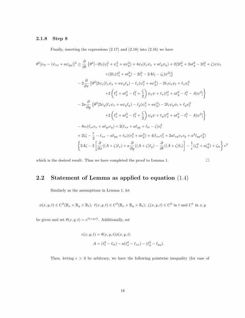
2.1.8 Step 8

Finally, inserting the expressions (2.17) and (2.18) into (2.16) we have

θ2[ψtt − (ψxx + aψyy)]2 ≥ ∂

∂t

θ2[−2`t(ψ

2t + ψ2


+(2`t(`2x + a`2y)− 2`3t − 2A`t − ζt)ψ2]

− 2

∂

∂x



2t

+2

(`2x + a`2y − `2t +

ζ

2

)ψxψ + `x(`2x + a`2y − `2t −A)ψ2]

− 2a

∂

∂y



2t

+2

(`2x + a`2y − `2t +

ζ

2

)ψyψ + `y(`2x + a`2y − `2t −A)ψ2]

− 8vt(`xtvx + a`ytvy) + 2(`xx + a`yy + `tt − ζ)v2

t

+ 2(ζ − ε

2− `xx − a`yy + `tt)(v

2x + av2


2y)

2Aζ − 2

[∂

∂x((A+ ζ)`x) + a

∂

∂y((A+ ζ)`y)− ∂

∂t((A+ ζ)`t)

]− 1

ε(ζ2x + aζ2

y ) + ζtt

v2

which is the desired result. Thus we have completed the proof to Lemma 1.

2.2 Statement of Lemma as applied to equation (1.4)

Similarly as the assumptions in Lemma 1, let

φ(x, y, t) ∈ C2(Rx × Ry × Rt); `(x, y, t) ∈ C3(Rx × Ry × Rt); ζ(x, y, t) ∈ C2 in t and C1 in x, y

be given and set θ(x, y, t) = e`(x,y,t). Additionally, set

v(x, y, t) = θ(x, y, t)φ(x, y, t)

A = (`2t − `tt)− a(`2x − `xx)− (`2y − `yy).

Then, letting ε > 0 be arbitrary, we have the following pointwise inequality (for ease of

18

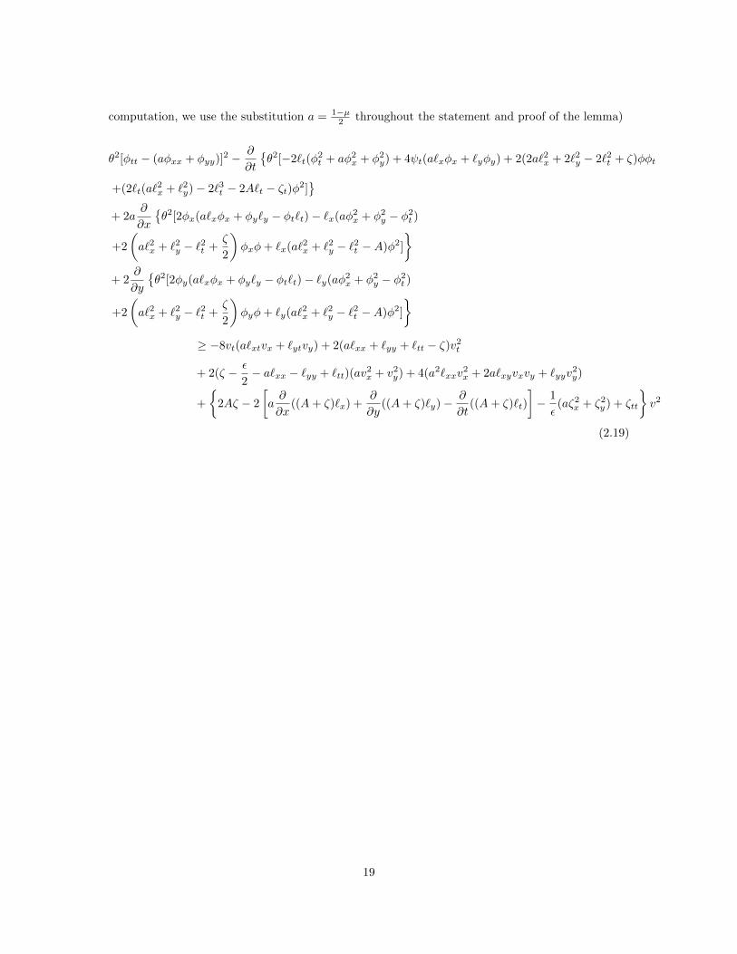
computation, we use the substitution a = 1−µ2 throughout the statement and proof of the lemma)

θ2[φtt − (aφxx + φyy)]2 − ∂

∂t

θ2[−2`t(φ

2t + aφ2

x + φ2y) + 4ψt(a`xφx + `yφy) + 2(2a`2x + 2`2y − 2`2t + ζ)φφt

+(2`t(a`2x + `2y)− 2`3t − 2A`t − ζt)φ2]

+ 2a

∂

∂x

θ2[2φx(a`xφx + φy`y − φt`t)− `x(aφ2

x + φ2y − φ2

t )

+2

(a`2x + `2y − `2t +

ζ

2

)φxφ+ `x(a`2x + `2y − `2t −A)φ2]

+ 2

∂

∂y

θ2[2φy(a`xφx + φy`y − φt`t)− `y(aφ2

x + φ2y − φ2

t )

+2

(a`2x + `2y − `2t +

ζ

2

)φyφ+ `y(a`2x + `2y − `2t −A)φ2]

≥ −8vt(a`xtvx + `ytvy) + 2(a`xx + `yy + `tt − ζ)v2

t

+ 2(ζ − ε

2− a`xx − `yy + `tt)(av

2x + v2

y) + 4(a2`xxv2x + 2a`xyvxvy + `yyv

2y)

+

2Aζ − 2

[a∂

∂x((A+ ζ)`x) +

∂

∂y((A+ ζ)`y)− ∂

∂t((A+ ζ)`t)

]− 1

ε(aζ2

x + ζ2y ) + ζtt

v2

(2.19)

19

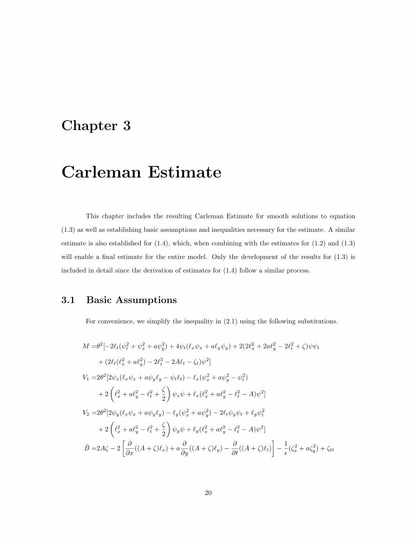
Chapter 3

Carleman Estimate

This chapter includes the resulting Carleman Estimate for smooth solutions to equation

(1.3) as well as establishing basic assumptions and inequalities necessary for the estimate. A similar

estimate is also established for (1.4), which, when combining with the estimates for (1.2) and (1.3)

will enable a final estimate for the entire model. Only the development of the results for (1.3) is

included in detail since the derivation of estimates for (1.4) follow a similar process.

3.1 Basic Assumptions

For convenience, we simplify the inequality in (2.1) using the following substitutions.

M =θ2[−2`t(ψ2t + ψ2


+ (2`t(`2x + a`2y)− 2`3t − 2A`t − ζt)ψ2]

V1 =2θ2[2ψx(`xψx + aψy`y − ψt`t)− `x(ψ2x + aψ2

y − ψ2t )

+ 2

(`2x + a`2y − `2t +

ζ

2

)ψxψ + `x(`2x + a`2y − `2t −A)ψ2]

V2 =2θ2[2ψy(`xψx + aψy`y)− `y(ψ2x + aψ2

y)− 2`tψyψt + `yψ2t

+ 2

(`2x + a`2y − `2t +

ζ

2

)ψyψ + `y(`2x + a`2y − `2t −A)ψ2]

B =2Aζ − 2

[∂

∂x((A+ ζ)`x) + a

∂

∂y((A+ ζ)`y)− ∂

∂t((A+ ζ)`t)

]− 1

ε(ζ2x + aζ2

y ) + ζtt

20

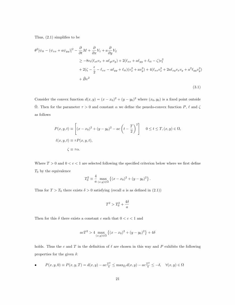
Thus, (2.1) simplifies to be


∂tM +

∂

∂xV1 + a

∂

∂yV2

≥ −8vt(`xtvx + a`ytvy) + 2(`xx + a`yy + `tt − ζ)v2t

+ 2(ζ − ε

2− `xx − a`yy + `tt)(v

2x + av2


2y)

+ Bv2

(3.1)

Consider the convex function d(x, y) = (x− x0)2 + (y − y0)2 where (x0, y0) is a fixed point outside

Ω. Then for the parameter τ > 0 and constant α we define the psuedo-convex function P , ` and ζ

as follows

P (x, y, t) ≡

[(x− x0)2 + (y − y0)2 − ac

(t− T

2

)2]

0 ≤ t ≤ T, (x, y) ∈ Ω,

`(x, y, t) ≡ τP (x, y, t),

ζ ≡ τα.

Where T > 0 and 0 < c < 1 are selected following the specified criterion below where we first define

T0 by the equivalence

T 20 ≡

4

amax

(x,y)∈Ω

(x− x0)2 + (y − y0)2

.

Thus for T > T0 there exists δ > 0 satisfying (recall a is as defined in (2.1))

T 2 > T 20 +

4δ

a

Then for this δ there exists a constant c such that 0 < c < 1 and

acT 2 > 4 max(x,y)∈Ω

(x− x0)2 + (y − y0)2

+ 4δ

holds. Thus the c and T in the definition of ` are chosen in this way and P exhibits the following

properties for the given δ:

• P (x, y, 0) ≡ P (x, y, T ) = d(x, y)− acT2

4 ≤ maxΩ d(x, y)− acT2

4 ≤ −δ, ∀(x, y) ∈ Ω

21

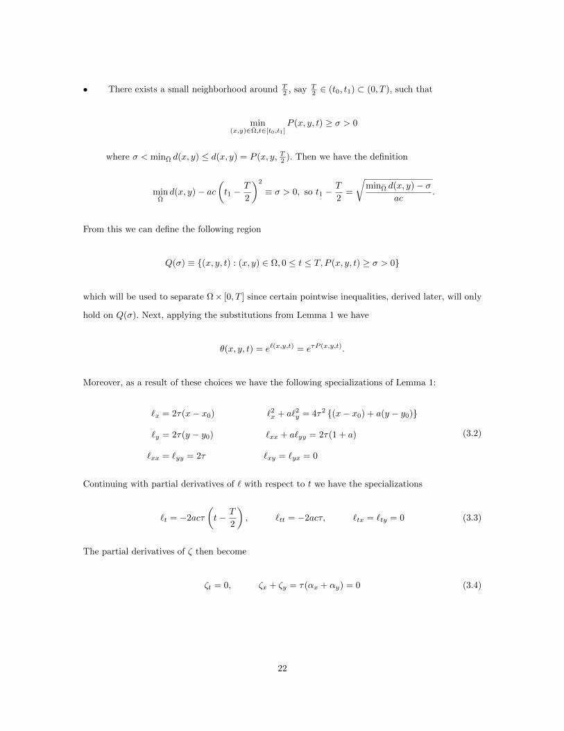
• There exists a small neighborhood around T2 , say T

2 ∈ (t0, t1) ⊂ (0, T ), such that

min(x,y)∈Ω,t∈[t0,t1]

P (x, y, t) ≥ σ > 0

where σ < minΩ d(x, y) ≤ d(x, y) = P (x, y, T2 ). Then we have the definition

minΩd(x, y)− ac

(t1 −

T

2

)2

≡ σ > 0, so t1 −T

2=

√minΩ d(x, y)− σ

ac.

From this we can define the following region

Q(σ) ≡ (x, y, t) : (x, y) ∈ Ω, 0 ≤ t ≤ T, P (x, y, t) ≥ σ > 0

which will be used to separate Ω× [0, T ] since certain pointwise inequalities, derived later, will only

hold on Q(σ). Next, applying the substitutions from Lemma 1 we have

θ(x, y, t) = e`(x,y,t) = eτP (x,y,t).

Moreover, as a result of these choices we have the following specializations of Lemma 1:

`x = 2τ(x− x0) `2x + a`2y = 4τ2 (x− x0) + a(y − y0)

`y = 2τ(y − y0) `xx + a`yy = 2τ(1 + a)

`xx = `yy = 2τ `xy = `yx = 0

(3.2)

Continuing with partial derivatives of ` with respect to t we have the specializations

`t = −2acτ

(t− T

2

), `tt = −2acτ, `tx = `ty = 0 (3.3)

The partial derivatives of ζ then become

ζt = 0, ζx + ζy = τ(αx + αy) = 0 (3.4)

22

3.2 A resulting pointwise inequality

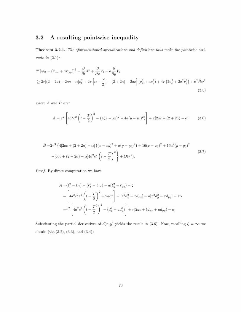
Theorem 3.2.1. The aforementioned specializations and definitions thus make the pointwise esti-

mate in (2.1):

θ2 [ψtt − (ψxx + aψyy)]2 − ∂

∂tM +

∂

∂xV1 + a

∂

∂yV2

≥ 2τ [(2 + 2a)− 2ac− α]v2t + 2τ

[α− ε

2τ− (2 + 2a)− 2ac

](v2x + av2

y) + 4τ(2v2x + 2a2v2

y

)+ θ2Bψ2

(3.5)

where A and B are:

A = τ2

[4a2c2

(t− T

2

)2

−(4(x− x0)2 + 4a(y − y0)2

)]+ τ [2ac+ (2 + 2a)− α] (3.6)

B =2τ3

4[2ac+ (2 + 2a)− α]((x− x0)2 + a(y − y0)2

)+ 16(x− x0)2 + 16a2(y − y0)2

−[6ac+ (2 + 2a)− α]4a2c2(t− T

2

)2

+O(τ2).(3.7)

Proof. By direct computation we have

A =(`2t − `tt)− (`2x − `xx)− a(`2y − `yy)− ζ

=

[4a2c2τ2

(t− T

2

)2

+ 2acτ

]− [τ2d2

x − τdxx]− a[τ2d2y − τdyy]− τα

=τ2

[4a2c2

(t− T

2

2)2

− (d2x + ad2

y)

]+ τ [2ac+ (dxx + adyy)− α]

Substituting the partial derivatives of d(x, y) yields the result in (3.6). Now, recalling ζ = τα we

obtain (via (3.2), (3.3), and (3.4))

23

2Aζ =2τ3α

[4a2c2

(t− T

2

)2

− (d2x + ad2

y)

]+ 2τ2α[2c+ (dxx + adyy)− α]

=2τ3α

[4a2c2

(t− T

2

)2

− 4((x− x0)2 + a(y − y0)2

)]+ 2τ2α[2ac+ (2 + 2a)− α]︸︷︷︸

O(τ2)

(A+ ζ)`x =τ3

[4a2c2

(t− T

2

)2

− (d2x + ad2

y)

]dx + τ2[2ac+ (dxx + adyy)− α]dx + τ2αdx

=τ3

[4a2c2

(t− T

2

)2

− 4((x− x0)2 + a(y − y0)2

)]dx + τ2[2ac+ (2 + 2a)]dx

∂

∂x[(A+ ζ)`x] =τ3

[4a2c2

(t− T

2

)2

− (d2x + ad2

y)

]dxx − τ3[2dxdxx + 2adydyx]dx +O(τ2)

=2τ3

[4a2c2

(t− T

2

)2

− 4((x− x0)2 + a(y − y0)2

)]− 16τ3(x− x0)2 +O(τ2)

(A+ ζ)`y =τ3

[4a2c2

(t− T

2

)2

− 4((x− x0)2 + a(y − y0)2

)]dy + τ2[2ac+ (2 + 2a)]dy

∂

∂y[(A+ ζ)`y] =2τ3

[4a2c2

(t− T

2

)2

− 4((x− x0)2 + a(y − y0)2

)]− 16aτ3(y − y0)2 +O(τ2)

∂

∂t[(A+ ζ)`t)] =2acτ3

[4a2c2

(t− T

2

)2

− (d2x + ad2

y)

]+ 2acτ3

(t− T

2

)2

8a2c2

=2acτ3

[4a2c2

(t− T

2

)2

− 4((x− x0)2 + a(y − y0)2

)]+ 16a3c3

(t− T

2

)2

=2acτ3

[12a2c2

(t− T

2

)2

− 4((x− x0)2 + a(y − y0)2

)]

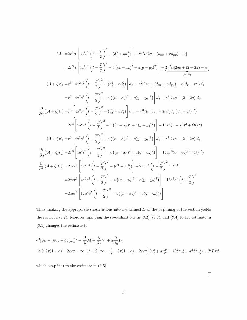
Thus, making the appropriate substitutions into the defined B at the beginning of the section yields

the result in (3.7). Morever, applying the specializations in (3.2), (3.3), and (3.4) to the estimate in

(3.1) changes the estimate to


∂tM +

∂

∂xV1 + a

∂

∂yV2

≥ 2 [2τ(1 + a)− 2acτ − τα] v2t + 2

[τα− ε

2− 2τ(1 + a)− 2acτ

](v2x + av2

y) + 4(2τv2x + a22τv2

y) + θ2Bψ2

which simplifies to the estimate in (3.5).

24

Since Theorem 3.2.1 holds for an arbitrary constant α, let

α ≡ (2 + 2a)− 2ac− a(1− k) for 0 < k < 1

such that (2 + 2a)− 2ac− α = a(1− k) > 0. Moreover, if we define γ by

γ ≡ α− 2ac− (2 + 2a) = −4ac− a(1− k) < 0

then we can choose a positive constant ρ by

ρ ≡ 4a+ γ = 4a− 4ac− a(1− k) > 0 for 4c− 3 < k < 1

and the inequality (2 + 2a)− 2ac− α ≥ ρ > 0 also holds.

Remark: While we have set ρ equivalent to 4a + γ, it is possible to set ρ slightly less than 4a + γ

for the purposes of the following corollary.

Thus we have the necessary conditions to establish the following pointwise inequality:

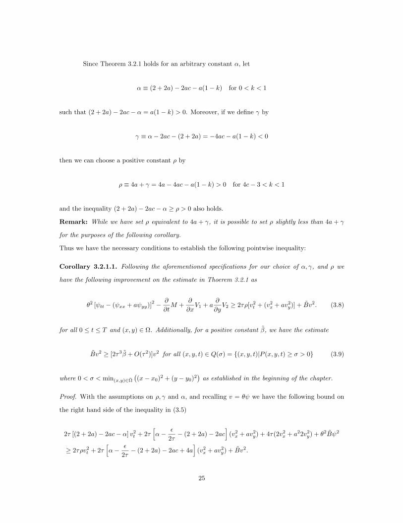
Corollary 3.2.1.1. Following the aforementioned specifications for our choice of α, γ, and ρ we

have the following improvement on the estimate in Thoerem 3.2.1 as

θ2 [ψtt − (ψxx + aψyy)]2 − ∂

∂tM +

∂

∂xV1 + a

∂

∂yV2 ≥ 2τρ[v2

t + (v2x + av2

y)] + Bv2. (3.8)

for all 0 ≤ t ≤ T and (x, y) ∈ Ω. Additionally, for a positive constant β, we have the estimate

Bv2 ≥ [2τ3β +O(τ2)]v2 for all (x, y, t) ∈ Q(σ) = (x, y, t)|P (x, y, t) ≥ σ > 0 (3.9)

where 0 < σ < min(x,y)∈Ω

((x− x0)2 + (y − y0)2

)as established in the beginning of the chapter.

Proof. With the assumptions on ρ, γ and α, and recalling v = θψ we have the following bound on

the right hand side of the inequality in (3.5)

2τ [(2 + 2a)− 2ac− α] v2t + 2τ

[α− ε

2τ− (2 + 2a)− 2ac

](v2x + av2

y) + 4τ(2v2x + a22v2

y) + θ2Bψ2

≥ 2τρv2t + 2τ

[α− ε

2τ− (2 + 2a)− 2ac+ 4a

](v2x + av2

y) + Bv2.

25

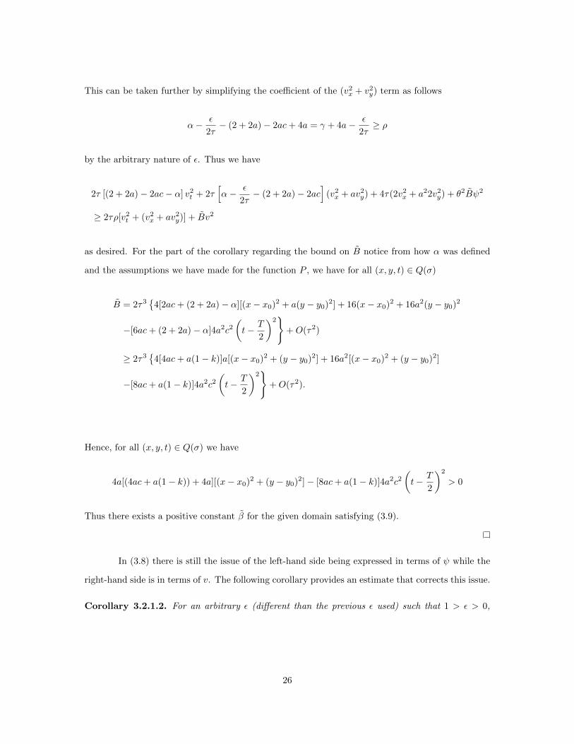
This can be taken further by simplifying the coefficient of the (v2x + v2

y) term as follows

α− ε

2τ− (2 + 2a)− 2ac+ 4a = γ + 4a− ε

2τ≥ ρ

by the arbitrary nature of ε. Thus we have

2τ [(2 + 2a)− 2ac− α] v2t + 2τ

[α− ε

2τ− (2 + 2a)− 2ac

](v2x + av2

y) + 4τ(2v2x + a22v2

y) + θ2Bψ2

≥ 2τρ[v2t + (v2

x + av2y)] + Bv2

as desired. For the part of the corollary regarding the bound on B notice from how α was defined

and the assumptions we have made for the function P , we have for all (x, y, t) ∈ Q(σ)

B = 2τ3

4[2ac+ (2 + 2a)− α][(x− x0)2 + a(y − y0)2] + 16(x− x0)2 + 16a2(y − y0)2

−[6ac+ (2 + 2a)− α]4a2c2(t− T

2

)2

+O(τ2)

≥ 2τ3

4[4ac+ a(1− k)]a[(x− x0)2 + (y − y0)2] + 16a2[(x− x0)2 + (y − y0)2]

−[8ac+ a(1− k)]4a2c2(t− T

2

)2

+O(τ2).

Hence, for all (x, y, t) ∈ Q(σ) we have

4a[(4ac+ a(1− k)) + 4a][(x− x0)2 + (y − y0)2]− [8ac+ a(1− k)]4a2c2(t− T

2

)2

> 0

Thus there exists a positive constant β for the given domain satisfying (3.9).

In (3.8) there is still the issue of the left-hand side being expressed in terms of ψ while the

right-hand side is in terms of v. The following corollary provides an estimate that corrects this issue.

Corollary 3.2.1.2. For an arbitrary ε (different than the previous ε used) such that 1 > ε > 0,

26

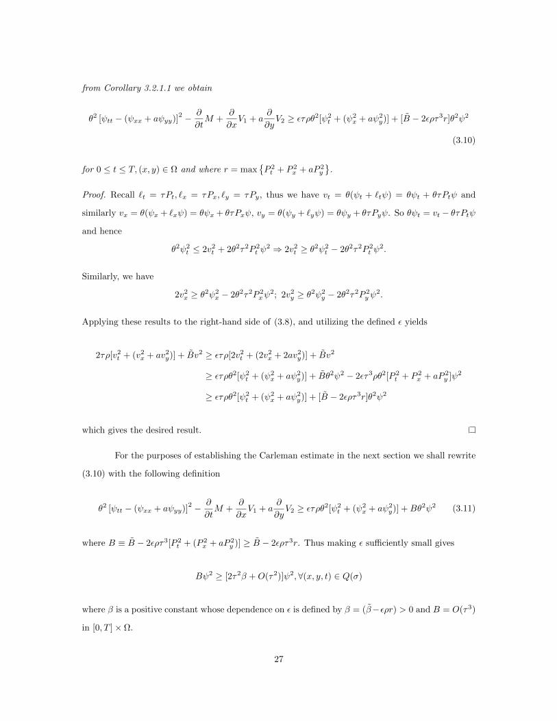
from Corollary 3.2.1.1 we obtain

θ2 [ψtt − (ψxx + aψyy)]2 − ∂

∂tM +

∂

∂xV1 + a

∂

∂yV2 ≥ ετρθ2[ψ2

t + (ψ2x + aψ2

y)] + [B − 2ερτ3r]θ2ψ2

(3.10)

for 0 ≤ t ≤ T, (x, y) ∈ Ω and where r = maxP 2t + P 2

x + aP 2y

.

Proof. Recall `t = τPt, `x = τPx, `y = τPy, thus we have vt = θ(ψt + `tψ) = θψt + θτPtψ and

similarly vx = θ(ψx + `xψ) = θψx + θτPxψ, vy = θ(ψy + `yψ) = θψy + θτPyψ. So θψt = vt − θτPtψ

and hence

θ2ψ2t ≤ 2v2

t + 2θ2τ2P 2t ψ

2 ⇒ 2v2t ≥ θ2ψ2

t − 2θ2τ2P 2t ψ

2.

Similarly, we have

2v2x ≥ θ2ψ2

x − 2θ2τ2P 2xψ

2; 2v2y ≥ θ2ψ2

y − 2θ2τ2P 2yψ

2.

Applying these results to the right-hand side of (3.8), and utilizing the defined ε yields

2τρ[v2t + (v2

x + av2y)] + Bv2 ≥ ετρ[2v2

t + (2v2x + 2av2

y)] + Bv2

≥ ετρθ2[ψ2t + (ψ2

x + aψ2y)] + Bθ2ψ2 − 2ετ3ρθ2[P 2

t + P 2x + aP 2

y ]ψ2

≥ ετρθ2[ψ2t + (ψ2

x + aψ2y)] + [B − 2ερτ3r]θ2ψ2

which gives the desired result.

For the purposes of establishing the Carleman estimate in the next section we shall rewrite

(3.10) with the following definition

θ2 [ψtt − (ψxx + aψyy)]2 − ∂

∂tM +

∂

∂xV1 + a

∂

∂yV2 ≥ ετρθ2[ψ2

t + (ψ2x + aψ2

y)] +Bθ2ψ2 (3.11)

where B ≡ B − 2ερτ3[P 2t + (P 2

x + aP 2y )] ≥ B − 2ερτ3r. Thus making ε sufficiently small gives

Bψ2 ≥ [2τ2β +O(τ2)]ψ2,∀(x, y, t) ∈ Q(σ)

where β is a positive constant whose dependence on ε is defined by β = (β−ερr) > 0 and B = O(τ3)

in [0, T ]× Ω.

27

3.3 Carleman estimate for equations (1.3) and (1.4)

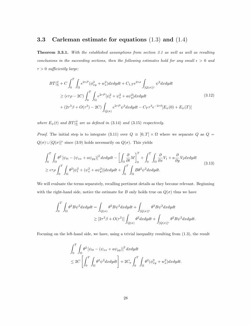
Theorem 3.3.1. With the established assumptions from section 3.1 as well as well as resulting

conclusions in the succeeding sections, then the following estimates hold for any small ε > 0 and

τ > 0 sufficiently large:

BT |ψΣ + C

∫ T

0

∫Ω

e2τP (φ2xy + w2

x)dxdydt+ C1,T e2τσ

∫[Q(σ)]c

ψ2dxdydt

≥ (ετρ− 2C)

∫ T

0

∫Ω

e2τP [ψ2t + ψ2

x + aψ2y]dxdydt

+ (2τ3β +O(τ2)− 2C)

∫Q(σ)

e2τPψ2dxdydt− CT τ3e−2τδ[Eψ(0) + Eψ(T )]

(3.12)

where Eψ(t) and BT |ψΣ are as defined in (3.14) and (3.15) respectively.

Proof. The initial step is to integrate (3.11) over Q ≡ [0, T ] × Ω where we separate Q as Q =

Q(σ) ∪ [Q(σ)]c since (3.9) holds necessarily on Q(σ). This yields

∫ T

0

∫Ω

θ2 [ψtt − (ψxx + aψyy)]2dxdydt−

[∫Ω

∂

∂tM

]T0

+

∫ T

0

∫Ω

∂

∂xV1 + a

∂

∂yV2dxdydt

≥ ετρ∫ T

0

∫Ω

θ2[ψ2t + (ψ2

x + aψ2y)]dxdydt+

∫ T

0

∫Ω

Bθ2ψ2dxdydt.

(3.13)

We will evaluate the terms separately, recalling pertinent details as they become relevant. Beginning

with the right-hand side, notice the estimate for B only holds true on Q(σ) thus we have

∫ T

0

∫Ω

θ2Bψ2dxdydt =

∫Q(σ)

θ2Bψ2dxdydt+

∫[Q(σ)]c

θ2Bψ2dxdydt

≥ [2τ2β +O(τ2)]

∫Q(σ)

θ2dxdydt+

∫[Q(σ)]c

θ2Bψ2dxdydt.

Focusing on the left-hand side, we have, using a trivial inequality resulting from (1.3), the result

∫ T

0

∫Ω

θ2 [ψtt − (ψxx + aψyy)]2dxdydt

≤ 2C

[∫ T

0

∫Ω

θ2ψ2dxdydt

]+ 2Ca

∫ T

0

∫Ω

θ2(φ2xy + w2

x)dxdydt.

28

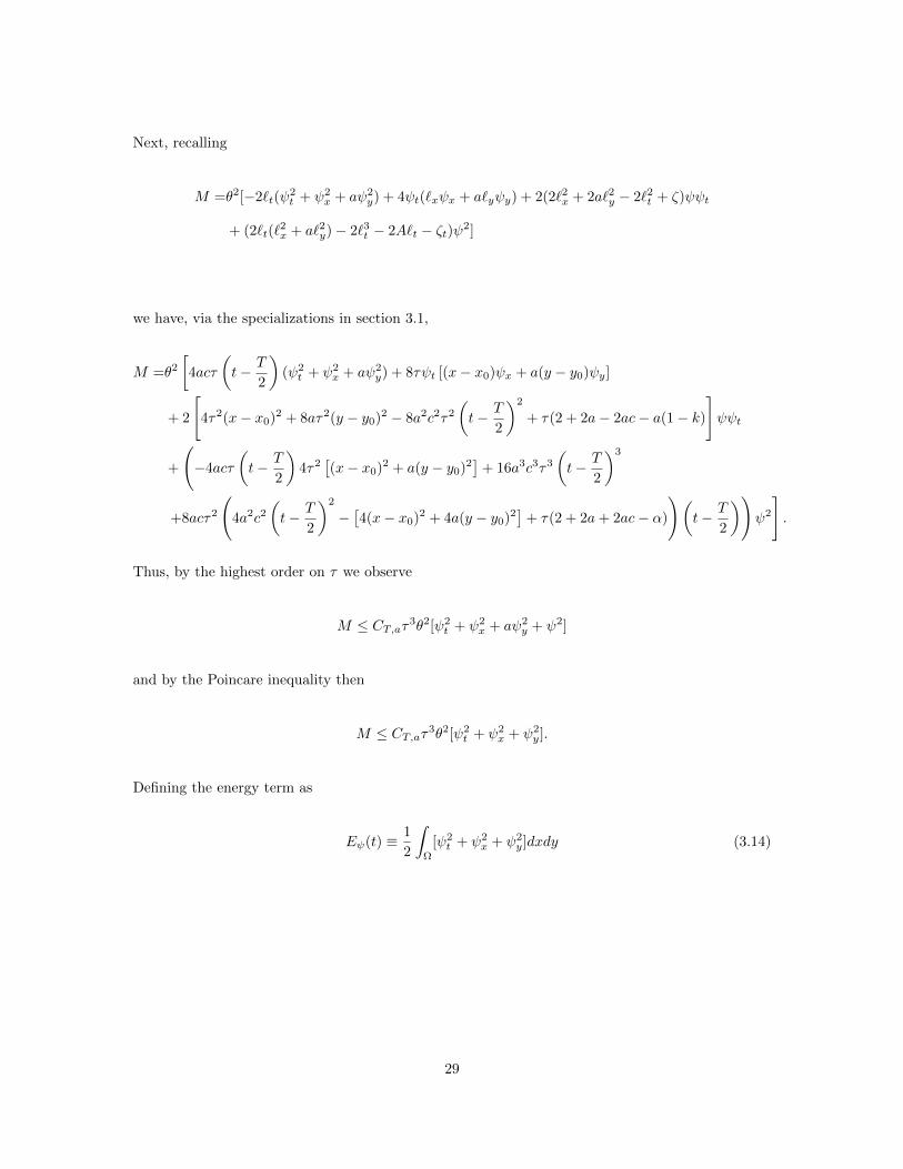
Next, recalling

M =θ2[−2`t(ψ2t + ψ2


+ (2`t(`2x + a`2y)− 2`3t − 2A`t − ζt)ψ2]

we have, via the specializations in section 3.1,

M =θ2

[4acτ

(t− T

2

)(ψ2t + ψ2

x + aψ2y) + 8τψt [(x− x0)ψx + a(y − y0)ψy]

+ 2

[4τ2(x− x0)2 + 8aτ2(y − y0)2 − 8a2c2τ2

(t− T

2

)2

+ τ(2 + 2a− 2ac− a(1− k)

]ψψt

+

(−4acτ

(t− T

2

)4τ2

[(x− x0)2 + a(y − y0)2

]+ 16a3c3τ3

(t− T

2

)3

+8acτ2

(4a2c2

(t− T

2

)2

−[4(x− x0)2 + 4a(y − y0)2

]+ τ(2 + 2a+ 2ac− α)

)(t− T

2

))ψ2

].

Thus, by the highest order on τ we observe

M ≤ CT,aτ3θ2[ψ2t + ψ2

x + aψ2y + ψ2]

and by the Poincare inequality then

M ≤ CT,aτ3θ2[ψ2t + ψ2

x + ψ2y].

Defining the energy term as

Eψ(t) ≡ 1

2

∫Ω

[ψ2t + ψ2

x + ψ2y]dxdy (3.14)

29

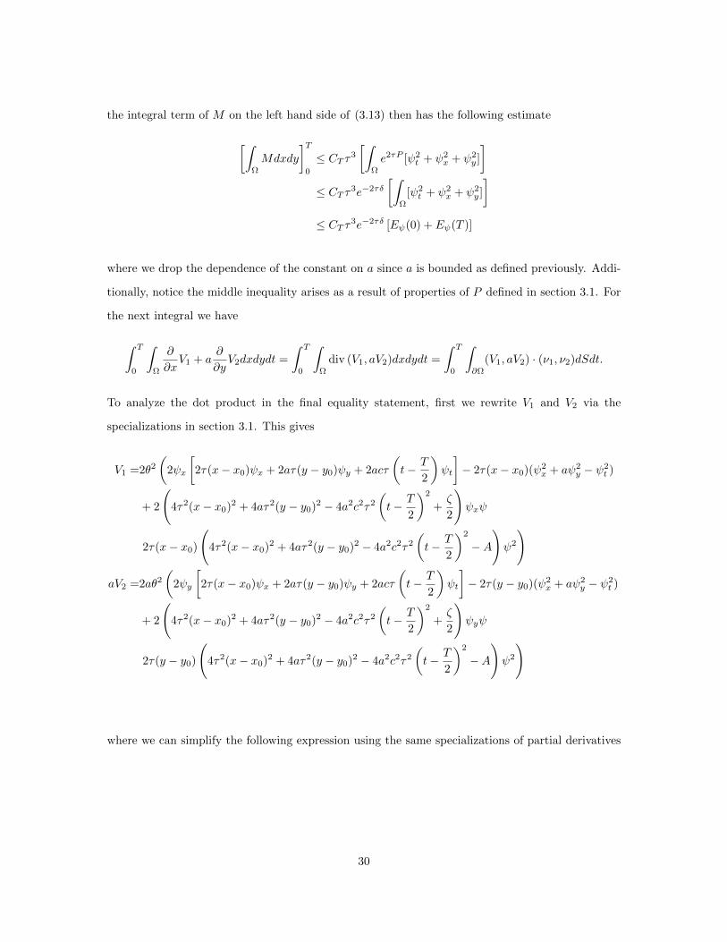
the integral term of M on the left hand side of (3.13) then has the following estimate

[∫Ω

Mdxdy

]T0

≤ CT τ3

[∫Ω

e2τP [ψ2t + ψ2

x + ψ2y]

]≤ CT τ3e−2τδ

[∫Ω

[ψ2t + ψ2

x + ψ2y]

]≤ CT τ3e−2τδ [Eψ(0) + Eψ(T )]

where we drop the dependence of the constant on a since a is bounded as defined previously. Addi-

tionally, notice the middle inequality arises as a result of properties of P defined in section 3.1. For

the next integral we have

∫ T

0

∫Ω

∂

∂xV1 + a

∂

∂yV2dxdydt =

∫ T

0

∫Ω

div (V1, aV2)dxdydt =

∫ T

0

∫∂Ω

(V1, aV2) · (ν1, ν2)dSdt.

To analyze the dot product in the final equality statement, first we rewrite V1 and V2 via the

specializations in section 3.1. This gives

V1 =2θ2

(2ψx

[2τ(x− x0)ψx + 2aτ(y − y0)ψy + 2acτ

(t− T

2

)ψt

]− 2τ(x− x0)(ψ2

x + aψ2y − ψ2

t )

+ 2

(4τ2(x− x0)2 + 4aτ2(y − y0)2 − 4a2c2τ2

(t− T

2

)2

+ζ

2

)ψxψ

2τ(x− x0)

(4τ2(x− x0)2 + 4aτ2(y − y0)2 − 4a2c2τ2

(t− T

2

)2

−A

)ψ2

)

aV2 =2aθ2

(2ψy

[2τ(x− x0)ψx + 2aτ(y − y0)ψy + 2acτ

(t− T

2

)ψt

]− 2τ(y − y0)(ψ2

x + aψ2y − ψ2

t )

+ 2

(4τ2(x− x0)2 + 4aτ2(y − y0)2 − 4a2c2τ2

(t− T

2

)2

+ζ

2

)ψyψ

2τ(y − y0)

(4τ2(x− x0)2 + 4aτ2(y − y0)2 − 4a2c2τ2

(t− T

2

)2

−A

)ψ2

)

where we can simplify the following expression using the same specializations of partial derivatives

30

of ` in the definition of A as

4τ2(x− x0)2 + 4aτ2(y − y0)2 − 4a2c2τ2

(t− T

2

)2

−A

=8τ2(x− x0)2 + 8aτ2(y − y0)2 − 8a2c2τ2

(t− T

2

)2

+ τ(α− 2ac− 2a− 2).

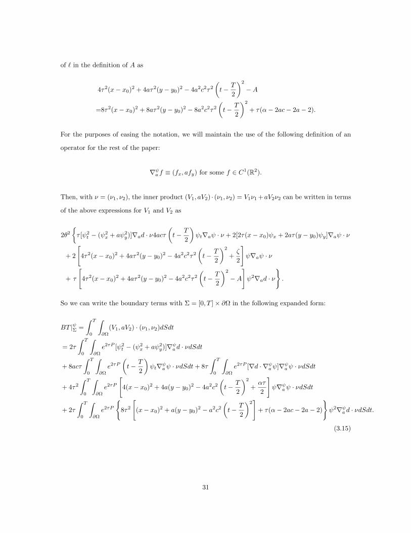
For the purposes of easing the notation, we will maintain the use of the following definition of an

operator for the rest of the paper:

∇ψa f ≡ (fx, afy) for some f ∈ C1(R2).

Then, with ν = (ν1, ν2), the inner product (V1, aV2) · (ν1, ν2) = V1ν1 +aV2ν2 can be written in terms

of the above expressions for V1 and V2 as

2θ2

τ [ψ2

t − (ψ2x + aψ2

y)]∇ad · ν4acτ

(t− T

2

)ψt∇aψ · ν + 2[2τ(x− x0)ψx + 2aτ(y − y0)ψy]∇aψ · ν

+ 2

[4τ2(x− x0)2 + 4aτ2(y − y0)2 − 4a2c2τ2

(t− T

2

)2

+ζ

2

]ψ∇aψ · ν

+ τ

[4τ2(x− x0)2 + 4aτ2(y − y0)2 − 4a2c2τ2

(t− T

2

)2

−A

]ψ2∇ad · ν

.

So we can write the boundary terms with Σ = [0, T ]× ∂Ω in the following expanded form:

BT |ψΣ =

∫ T

0

∫∂Ω

(V1, aV2) · (ν1, ν2)dSdt

= 2τ

∫ T

0

∫∂Ω

e2τP [ψ2t − (ψ2

x + aψ2y)]∇ψa d · νdSdt

+ 8acτ

∫ T

0

∫∂Ω

e2τP

(t− T

2

)ψt∇ψaψ · νdSdt+ 8τ

∫ T

0

∫∂Ω

e2τP [∇d · ∇ψaψ]∇ψaψ · νdSdt

+ 4τ2

∫ T

0

∫∂Ω

e2τP

[4(x− x0)2 + 4a(y − y0)2 − 4a2c2

(t− T

2

)2

+ατ

2

]ψ∇ψaψ · νdSdt

+ 2τ

∫ T

0

∫∂Ω

e2τP

8τ2

[(x− x0)2 + a(y − y0)2 − a2c2

(t− T

2

)2]

+ τ(α− 2ac− 2a− 2)

ψ2∇ψa d · νdSdt.

(3.15)

31

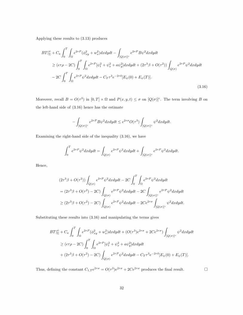
Applying these results to (3.13) produces

BT |ψΣ + Ca

∫ T

0

∫Ω

e2τP (φ2xy + w2

x)dxdydt−∫

[Q(σ)]ce2τPBψ2dxdydt

≥ (ετρ− 2C)

∫ T

0

∫Ω

e2τP [ψ2t + ψ2

x + aψ2y]dxdydt+ (2τ3β +O(τ2))

∫Q(σ)

e2τPψ2dxdydt

− 2C

∫ T

0

∫Ω

e2τPψ2dxdydt− CT τ3e−2τδ[Eψ(0) + Eψ(T )].

(3.16)

Moreover, recall B = O(τ3) in [0, T ] × Ω and P (x, y, t) ≤ σ on [Q(σ)]c. The term involving B on

the left-hand side of (3.16) hence has the estimate

−∫

[Q(σ)]ce2τPBψ2dxdydt ≤ e2τσO(τ3)

∫[Q(σ)]c

ψ2dxdydt.

Examining the right-hand side of the inequality (3.16), we have

∫ T

0

e2τPψ2dxdydt =

∫Q(σ)

e2τPψ2dxdydt+

∫[Q(σ)]c

e2τPψ2dxdydt.

Hence,

(2τ3β +O(τ2))

∫Q(σ)

e2τPψ2dxdydt− 2C

∫ T

0

∫Ω

e2τPψ2dxdydt

= (2τ3β +O(τ2)− 2C)

∫Q(σ)

e2τPψ2dxdydt− 2C

∫[Q(σ)]c

e2τPψ2dxdydt

≥ (2τ3β +O(τ2)− 2C)

∫Q(σ)

e2τPψ2dxdydt− 2Ce2τσ

∫[Q(σ)]c

ψ2dxdydt.

Substituting these results into (3.16) and manipulating the terms gives

BT |ψΣ + Ca

∫ T

0

∫Ω

e2τP (φ2xy + w2

x)dxdydt+ (O(τ3)e2τσ + 2Ce2τσ)

∫[Q(σ)]c

ψ2dxdydt

≥ (ετρ− 2C)

∫ T

0

∫Ω

e2τP [ψ2t + ψ2

x + aψ2y]dxdydt

+ (2τ3β +O(τ2)− 2C)

∫Q(σ)

e2τPψ2dxdydt− CT τ3e−2τδ[Eψ(0) + Eψ(T )].

Thus, defining the constant C1,T e2τσ = O(τ3)e2τσ + 2Ce2τσ produces the final result.

32

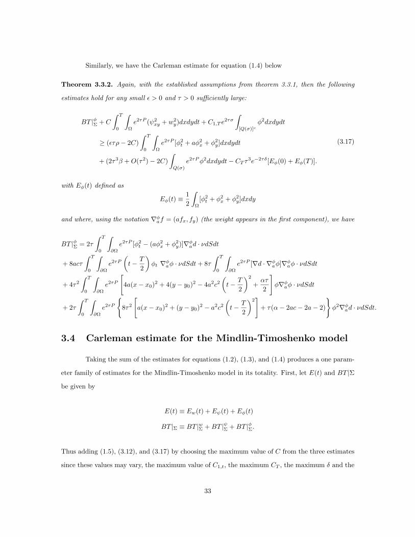
Similarly, we have the Carleman estimate for equation (1.4) below

Theorem 3.3.2. Again, with the established assumptions from theorem 3.3.1, then the following

estimates hold for any small ε > 0 and τ > 0 sufficiently large:

BT |φΣ + C

∫ T

0

∫Ω

e2τP (ψ2xy + w2

y)dxdydt+ C1,T e2τσ

∫[Q(σ)]c

φ2dxdydt

≥ (ετρ− 2C)

∫ T

0

∫Ω

e2τP [φ2t + aφ2

x + φ2y]dxdydt

+ (2τ3β +O(τ2)− 2C)

∫Q(σ)

e2τPφ2dxdydt− CT τ3e−2τδ[Eφ(0) + Eφ(T )].

(3.17)

with Eφ(t) defined as

Eφ(t) ≡ 1

2

∫Ω

[φ2t + φ2

x + φ2y]dxdy

and where, using the notation ∇φaf = (afx, fy) (the weight appears in the first component), we have

BT |φΣ = 2τ

∫ T

0

∫∂Ω

e2τP [φ2t − (aφ2

x + φ2y)]∇φad · νdSdt

+ 8acτ

∫ T

0

∫∂Ω

e2τP

(t− T

2

)φt ∇φaφ · νdSdt+ 8τ

∫ T

0

∫∂Ω

e2τP [∇d · ∇φaφ]∇φaφ · νdSdt

+ 4τ2

∫ T

0

∫∂Ω

e2τP

[4a(x− x0)2 + 4(y − y0)2 − 4a2c2

(t− T

2

)2

+ατ

2

]φ∇φaφ · νdSdt

+ 2τ

∫ T

0

∫∂Ω

e2τP

8τ2

[a(x− x0)2 + (y − y0)2 − a2c2

(t− T

2

)2]

+ τ(α− 2ac− 2a− 2)

φ2∇φad · νdSdt.

3.4 Carleman estimate for the Mindlin-Timoshenko model

Taking the sum of the estimates for equations (1.2), (1.3), and (1.4) produces a one param-

eter family of estimates for the Mindlin-Timoshenko model in its totality. First, let E(t) and BT |Σ

be given by

E(t) ≡ Ew(t) + Eψ(t) + Eφ(t)

BT |Σ ≡ BT |wΣ +BT |ψΣ +BT |φΣ.

Thus adding (1.5), (3.12), and (3.17) by choosing the maximum value of C from the three estimates

since these values may vary, the maximum value of C1,t, the maximum CT , the maximum δ and the

33

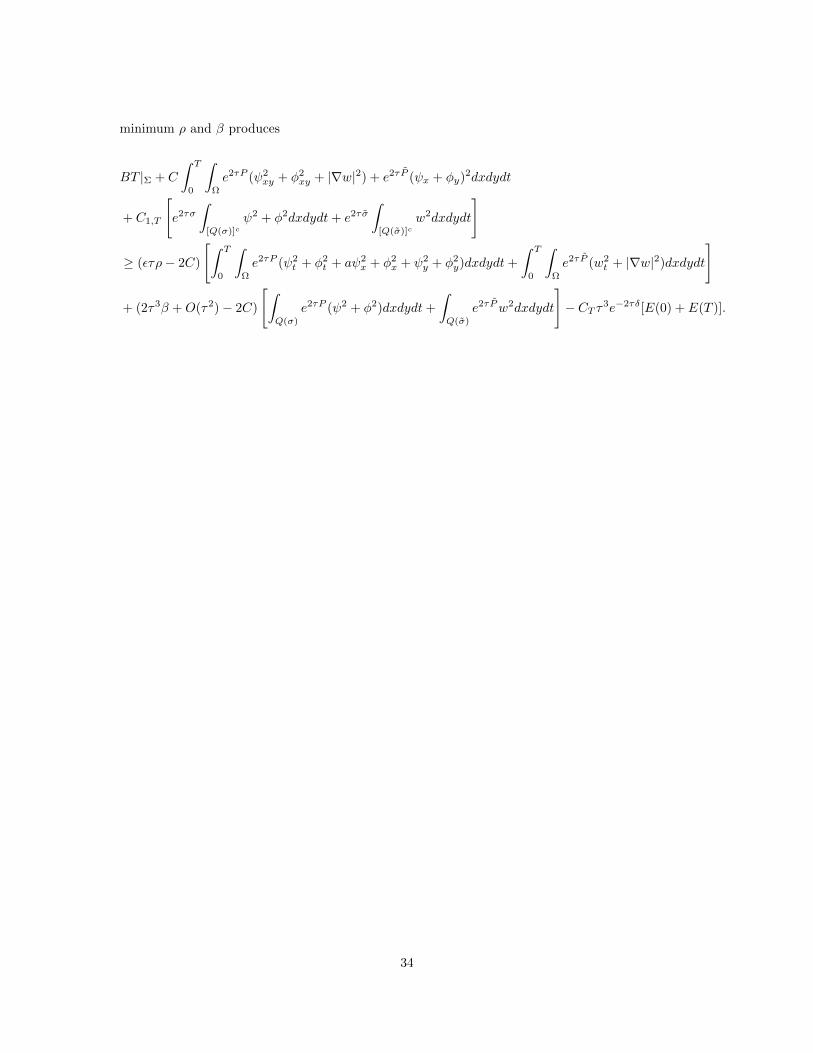
minimum ρ and β produces

BT |Σ + C

∫ T

0

∫Ω

e2τP (ψ2xy + φ2

xy + |∇w|2) + e2τP (ψx + φy)2dxdydt

+ C1,T

[e2τσ

∫[Q(σ)]c

ψ2 + φ2dxdydt+ e2τσ

∫[Q(σ)]c

w2dxdydt

]

≥ (ετρ− 2C)

[∫ T

0

∫Ω

e2τP (ψ2t + φ2

t + aψ2x + φ2

x + ψ2y + φ2

y)dxdydt+

∫ T

0

∫Ω


]

+ (2τ3β +O(τ2)− 2C)

[∫Q(σ)

e2τP (ψ2 + φ2)dxdydt+

∫Q(σ)

e2τPw2dxdydt

]− CT τ3e−2τδ[E(0) + E(T )].

34

Chapter 4

Conclusions and Discussion

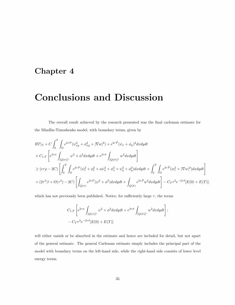
The overall result achieved by the research presented was the final carleman estimate for

the Mindlin-Timoshenko model, with boundary terms, given by

BT |Σ + C

∫ T

0

∫Ω

e2τP (ψ2xy + φ2

xy + |∇w|2) + e2τP (ψx + φy)2dxdydt

+ C1,T

[e2τσ

∫[Q(σ)]c


∫[Q(σ)]c

w2dxdydt

]

≥ (ετρ− 2C)

[∫ T

0

∫Ω

e2τP (ψ2t + φ2

t + aψ2x + φ2

x + ψ2y + φ2

y)dxdydt+

∫ T

0

∫Ω


]

+ (2τ3β +O(τ2)− 2C)

[∫Q(σ)

e2τP (ψ2 + φ2)dxdydt+

∫Q(σ)

e2τPw2dxdydt

]− CT τ3e−2τδ[E(0) + E(T )].

which has not previously been published. Notice, for sufficiently large τ , the terms

C1,T

[e2τσ

∫[Q(σ)]c


∫[Q(σ)]c

w2dxdydt

];

− CT τ3e−2τδ[E(0) + E(T )]

will either vanish or be absorbed in the estimate and hence are included for detail, but not apart

of the general estimate. The general Carleman estimate simply includes the principal part of the

model with boundary terms on the left-hand side, while the right-hand side consists of lower level

energy terms.

35

4.1 Purpose of the Estimate

The original purpose of Carleman estimates were mostly to prove unique continuation theo-

rems, but this has evolved over time. The inclusion of the exact boundary terms make this estimate

useful for boundary control problems in the field of control theory. Observability for the model would

also need to be established since the model is different enough from the traditional wave equation

that this would not be guaranteed. Another application would be utilizing the estimate in exploring

the inverse problem for this model.

4.2 Recommendations for Further Research

The next step will be to pursue observability and, hence, exact controllability of the Mindlin-

Timoshenko model, which would open the possibility of a myriad of applications for this model. Due

to the nature of the model’s application to the mechanics of vibrating, thin plates, engineers and

applied mathematicians who work with such models could use the information to further there own

research. These systems of thin plates under high frequency vibrations have appeared in proximity

sensors and other electronic devices so the implications are broad [10].

36

References

[1] I. Carleman. Sur un probleme d’unicite pour les systemes d’equations aux derivees partielles adeux variables independantes. Ark. Mat. Astr. Fyd., 2B:1–9, 1939.

[2] M. Grobbelaar-Van Dalsen. Strong stabilization of models incorporating the thermoelasticreissner-mindlin plate equations with second sound. Applicable Analysis, 90(9):1419–1449,September 2011.

[3] L. Hoermander. Linear Partial Differential Operators, volume 10. Springer-Verlag, 1969.

[4] J.E. Lagnese. Boundary Stabilization of Thin Plates, volume 10 of SIAM Studies in AppliedMathematics. SIAM, Philadelphia, 1989.

[5] I. Lasiecka and R. Triggiani. Carleman estimates and exact controllability for a system ofcoupled, nonconservative second-order hyperbolic equations. Marcel Dekker Lectures NotesPure Appl. Math., 188:215–245, 1997.

[6] I. Lasiecka, R. Triggiani, and X. Zhang. Nonconservative wave equations with unobservedneumann b.c.: Global uniqueness and observability in one shot. Contemporary Mathematics,268:227–326, 2000.

[7] M.M. Lavrentev, V.G. Romanov, and S.P. Shishataskii. Ill-Posed Problems of MathematicalPhysics and Analysis, volume 64. Amer. Math. Soc., Providence, RI, 1986.

[8] S. Lui. Personal conversations, 2017. Clemson University.

[9] R.D. Mindlin. Thickness-shear and flexural vibrations of crystal plates. J. Appl. Phy., 22:316–322, 1951.

[10] P. Pei, M.A. Rammaha, and D. Toundykov. Well-posedness and stability of a mindlin-timoshenko plate model with damping and sources. In V.V. Mityushev and M.V. Ruzhansky,editors, Current Trends in Analysis and Its Applications, pages 307–314, Switzerland, 2015.ISAAC Congress, Springer International.

[11] E. Reissner. The effect of transverse shear deformation on the bending of elastic plates. Philos.Mag., 42:744–746, 1921.

[12] H.D. Fernandez Sare. On the stability of mindlin-timoshenko plates. Quarterly of AppliedMathematics, LXVII(2):249–263, March 2009.

[13] M.A. Jorge Silva, T.F. Ma, and J.E. Munoz Rivera. Mindlin-timoshenko systems with kelvin-voigt: analyticity and optimal decay rates. Journal of Mathematical Analysis and Applications,417:164–179, 2014.

[14] D. Tataru. Boundary controllability for conservative pde’s. Applied Mathematics & Optimiza-tion, 31:257–295, December 1995.

37

[15] S. Timoshenko. On the correction of shear in the differential equation for transverse vibrationsof prismatic bars. Philos. Mag., 42:744–746, 1921.

38

Documents

A Carleman type estimate for the Mindlin-Timoshenko plate