A Bulk Microphysics Parameterization with Multiple Ice ...u0758091/MPschemes/Strakamansell2005.pdf · A Bulk Microphysics Parameterization with Multiple Ice Precipitation Categories

A Bulk Microphysics Parameterization with Multiple Ice Precipitation Categories

JERRY M. STRAKA

School of Meteorology, The University of Oklahoma, Norman, Oklahoma

EDWARD R. MANSELL

Cooperative Institute for Mesoscale Meteorological Studies, The University of Oklahoma, Norman, Oklahoma

(Manuscript received 9 September 2003, in final form 27 September 2004)

ABSTRACT

A single-moment bulk microphysics scheme with multiple ice precipitation categories is described. It has2 liquid hydrometeor categories (cloud droplets and rain) and 10 ice categories that are characterized byhabit, size, and density—two ice crystal habits (column and plate), rimed cloud ice, snow (ice crystalaggregates), three categories of graupel with different densities and intercepts, frozen drops, small hail, andlarge hail. The concept of riming history is implemented for conversions among the graupel and frozendrops categories. The multiple precipitation ice categories allow a range of particle densities and fallvelocities for simulating a variety of convective storms with minimal parameter tuning. The scheme isapplied to two cases—an idealized continental multicell storm that demonstrates the ice precipitationprocess, and a small Florida maritime storm in which the warm rain process is important.

1. Introduction

Numerical modeling of storms is a mature field thathas a history as long as the computers that have beencapable of handling the computations. As computershave grown in power, researchers have added morecomplex and comprehensive physics into models thatare being applied at ever-greater spatial resolution. Abalance must still be struck between greater resolutionand greater detail in the microphysical treatment—bothof which result in increased computation. Microphysicsschemes are generally categorized into “bulk” and“bin” approaches. The bin approach divides the par-ticle spectrum into 20 or more size or mass bins (e.g.,Berry 1967). A main disadvantage of bin microphysicsis the memory and storage requirements for largestorms in three dimensions, which becomes evengreater if an electric charge is added for electrificationstudies. Bulk schemes, on the other hand, specify afunctional form for the particle distribution and usuallypredict one or two characteristics of a particle categorysuch as the total mass (mixing ratio) and concentration.

Over the past three or more decades cloud modelershave developed numerous types of bulk cloud and pre-

cipitation schemes. The simplest are saturation-adjust-ment schemes. The inadequacy of these very simpleschemes for studying phenomena such as the develop-ment of cloud or rain led to parameterizations devel-oped by Kessler (1969) and Simpson and Wiggert(1969). These predicted vapor, cloud droplets, and rain.Further expansion to study ice physics encouraged Wis-ner et al. (1972), Ogura and Takahashi (1973), Cotton(1972a), Cotton et al. (1982), Lin et al. (1983), and Rut-ledge and Hobbs (1984), to name a few, to developschemes with two or three ice categories to capturesome of the important physics associated with ice inprecipitation production. These were expandedthrough the 1990s to take models to a greater under-standing of liquid and ice physics with elaborate cloudand precipitation physics schemes and multiple mo-ments. Ferrier (1994) presented a six-class two-momentscheme that included separate graupel and hail/frozendrops categories (and liquid water fraction on wet ice),improved treatments of some interactions, and otherenhancements, such as a formulation that used gener-alized gamma distributions for describing particle spec-tra. The seven-class model of Walko et al. (1995) andMeyers et al. (1997) also had separate graupel and hailcategories and additionally had separate snow and ag-gregates categories.

Inspired by the detailed cloud and precipitation pathdiagram of Braham (1968), a five-class scheme(Gilmore et al. 2004a, hereinafter GSR04) has beengreatly expanded to include more hydrometeor habits

Corresponding author address: Dr. Edward Mansell, NationalSevere Storms Laboratory/CIMMS, 1313 Halley Circle, Norman,OK 73069.E-mail: [email protected]

APRIL 2005 S T R A K A A N D M A N S E L L 445

© 2005 American Meteorological Society

JAM2211

than any previous bulk parameterization models to ourknowledge. This responds to the need for a more gen-eral parameterization to simulate convective cloudsover a range of latitudes (Tropics to high plains) as wellas other precipitation systems that are not well simu-lated by a typical five-class scheme. For example, Fer-rier et al. (1995) showed the advantages of separategraupel and hail categories for producing more realisticstorm characteristics. The scheme presented here hasan emphasis on multiple ice categories in order to pro-vide a smoother transition in physical characteristics,especially particle density and terminal velocity, as par-ticles freeze or rime. The habits included in the modelare cloud droplets, rain, ice crystals (three habits), ag-gregates/snow, graupel (three densities), frozen drops,and hail (small and large). Although the present paperdescribes a single-moment model, prediction of numberconcentration (double-moment model) is under devel-opment with optional prediction of mean diameter(triple-moment model), following Clark (1974).

Another motivation for the new expanded schemewas for studies of thunderstorm electrification. A hostof laboratory and field studies have identified rebound-ing collisions between ice particles as the primarymechanism of charge separation in storms (MacGor-man and Rust 1998, and references therein). Because ofthis primary dependence on ice particle interactions, adetailed ice microphysical package is desirable. Otherschemes may be adequate for small storms (e.g., Hels-don and Farley 1987; Helsdon et al. 2001), but becomeless realistic for larger, more complex storms or must betuned for a particular case. A scheme that needs little orno parameter tuning between storm types allows for theelectrification parameterizations to remain constant aswell. For example, charge separation rates are sensitiveto particle fall speeds (more specifically, to collisionimpact speeds). With multiple precipitation ice types,fall speed variations can arise naturally as particles areconverted between types, rather than artificially by tun-ing the particle characteristics for a particular simula-tion.

It is hoped with this new scheme, designed for use inthree-dimensional cloud-resolving models, that it mightbe reasonable to make comparisons with radar, includ-ing polarimetric radar (Straka et al. 2000). Also, studiesof other closely related phenomena, such as electrifica-tion and lightning, might be advanced. Last, the modelphysics might help to make studies of severe convectiontake hold of a new view of what might be causing, forexample, large hail, large quantities of hail, rear-flankdowndrafts, microbursts, and tornadoes. In the follow-ing parts of the paper the model is described.

2. 10-ICE microphysics model

The new microphysics package is in many regards asubstantial expansion and improvement of Straka’s

three-class bulk ice (3-ICE) scheme in GSR04, which isbased on Lin et al. (1983). The newer 10-class bulk ice(10-ICE) scheme also uses a bulk representation foreach hydrometeor type. It has the same two liquid hy-drometeor categories (cloud droplets and rain) as the3-ICE scheme and 10 ice categories that are character-ized by habit and size—two pristine ice crystal habits[column ice (CI) and plate ice (IP), which have differ-ent minimum diameters for riming], rimed cloud ice(IR), snow (SA; here considered to be ice crystal ag-gregates), three categories of graupel with differentcharacteristics [low-density graupel (GL), medium-density graupel (GM), and high-density graupel (GH)],frozen drops (F), small hail (H), and large hail (HL;Table 1. Thus, there are six large ice precipitation types(three graupel, frozen drops, and two hail) instead ofthe single graupel/hail category provided in the 3-ICEscheme, which includes only cloud ice, aggregates, andhail. The extra ice hydrometeor types were added tobetter represent the range of precipitation ice charac-teristics in a convective storm system. It was also de-veloped to improve the treatment of conversions fromone ice species to another with changes in habit, den-sity, and terminal velocity.

The basic set of processes presented by GSR04 ap-plies to the expanded scheme with a few exceptions.For example, the equation for accretion of cloud waterby hail in GSR04 takes the same form for the graupel,frozen drops, and hail categories. Cloud droplets andcloud ice crystals (columns and plates) are treated asmonodisperse (MD) distributions, and precipitationparticles are assumed to have inverse exponential (IE)size distributions as in GSR04,

nx�D� � no,xe�D�Dn,x, �1�

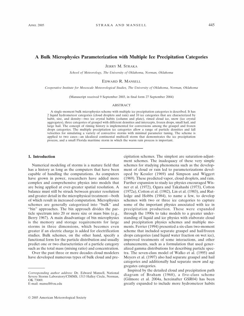
where nx(D) (m�4) is the number concentration of par-ticles (per meter) with diameter D of hydrometeor cat-egory x, and no,x is the fixed intercept value. Note thatDn here is the characteristic diameter (e.g., as in Cottonet al. 1986), which is the inverse of the slope � of the IEdistribution, so that Dn � ��1. Table 1 lists the numberconcentration intercepts and the particle density foreach hydrometeor category. Mass-weighted terminalfall speeds are plotted in Fig. 1 for an air density of1.0 kg m�3.

A number of microphysical schemes now use gammafunctions to describe the size distributions of one ormore hydrometeor type (e.g., Ziegler 1985; Ferrier1994; Walko et al. 1995; Meyers et al. 1997), and log-normal functions have also been used (Clark 1976;Feingold and Levin 1986; Feingold et al. 1998). Thegamma function has greater flexibility, especially intreating the small-diameter end of the size spectrum.Smith (2003) pointed out that observations are poor forsmall particles, making it difficult to distinguish obser-vationally between the different predictions of gammaand exponential distributions. He further questioned

446 J O U R N A L O F A P P L I E D M E T E O R O L O G Y VOLUME 44

whether the extra complication of a gamma functiondistribution is justifiable from a verification point ofview. While the discussion by Smith (2003) somewhatjustifies the use of exponential distributions for precipi-tation hydrometeors in the present version of the 10-ICE scheme, gamma functions would be more theoret-ically consistent for certain hydrometeor types. For ex-ample, the small- and large-hail categories each assumea minimum particle size (5 and 20 mm, respectively).Such changes are planned for future versions of the10-ICE scheme. Other planned improvements are touse general gamma functions distributions for cloudparticles (droplets and crystals) and to predict numberconcentrations of all ice species.

The hydrometeor mixing ratio conservation equationis (in vector form)

�q

�t� �

1

�a�� · ��aqV� � q� · ��aV�� · �Kh�q�

�1

�a

��V�aq�

�z� S. �2�

The first two terms on the right-hand side (in brackets)represent advection (the model scheme uses the fluxformulation), followed by the turbulent mixing and fall-out terms. The microphysical source and sink terms (S)

include the following form and phase changes: conden-sation and evaporation, deposition and sublimation,freezing and melting, autoconversion of cloud to rain,ice aggregation, ice nucleation, and collection growth.To compute the source and sink terms, the model em-ploys parameterized expressions for cloud microphysi-cal processes proceeding from approaches of Lin et al.(1983), Cotton et al. (1986), Meyers et al. (1992), Fer-rier (1994), and others, as described below.

Many processes are treated in 10-ICE in the samemanner as in GSR04. These processes include, but arenot limited to, stochastic freezing of raindrops (similarto Wisner et al. 1972, which is based on Bigg 1953), wetgrowth (shedding) of hail (and high-density graupel andfrozen drops, but not snow and low- and medium-density graupel), vapor deposition and sublimation,saturation adjustment, melting, and evaporation.

a. Collection rate equations

The collection rate (qxacy) of one hydrometeor spe-cies (y) by another (x) follows GSR04. [The nomencla-ture has the interpretation qxacy � rate of change ofmixing ratio q of species x when it collects or accretes(ac) species y.] In the following expressions, Dn is thecharacteristic diameter (inverse slope) of an IE Mar-shall–Palmer size distribution, and D is the diameter for

TABLE 1. Intercept and density values and fall velocity (V) information for hydrometeor categories. All units have been convertedto SI. The Stokes law for cloud droplet fall velocity is valid for the allowed size range of 5–50 10�6 m. The kinematic viscosity isgiven in appendix B. Ice plate and column fall velocities are from Davis and Auer (1974). Other fall velocity constants are ar � 842.0and br � 0.8 (Liu and Orville 1969) and cs � 12.4 and ds � 0.42 (Potter 1991). The base-state air density is denoted by �a, and thereference air density is �o � 1.225 kg m�3.

Category Abbreviation Intercept no,x (m�4) Density (kg m�3) V or CD

Cloud droplets W — 1000 g��w � �a�Dw2

18�a�

Column ice CI — 900131.6 Dci

0.824��o

�a

Plate ice IP — 90049 420 Dip

1.4150��o

�a

Rimed ice IR 1.0 108 300 cs��4 � ds�D n,irds

6.0 ��o

�a

Rain R 8.0 106 1000 ar��4 � br�D n,rbr

6.0 ��o

�a

Snow aggregate SA 8.0 106 100 cs��4 � ds�D n,sds

6.0 ��o

�a

Graupel (low) GL 4.0 105 300 0.8

Graupel (medium) GM 4.0 105 500 0.8

Graupel (high) GH 4.0 105 700 0.6

Frozen drops F 4.0 105 800 0.45

Small hail H 4.0 104 800 0.45

Large hail HL 1.0 103 900 0.45


an MD distribution. Although number concentration nx

is not predicted, it is diagnosed (nx � no,xDn,x) and usedto calculate collision rates. Relevant equations explic-itly include nx for an easier future upgrade to two pre-dicted moments. The collision rates also can be used forelectrical charge transfer rates. For convenience, theaccretion rate equations from GSR04 are repeatedhere. A future improvement will be the replacement ofthe collection equations with a more accurate method,such as that of Verlinde et al. (1990) or Ferrier (1994).

For an IE distribution (xe) collecting an MD distri-bution (ym), the mixing ratio collection rate qxeacym is

qxeacym ��

4Exyqynx |Vx � Vm,y |

��3�Dn,x2 � 2��2�Dn,xDy � ��1�Dy

2�, �3�

where � is the complete Gamma function, V is the(mass weighted) mean fall speed of an IE distribution,and Vm is the fall speed of the MD particles.

For an IE distribution (xe) accreting another IE dis-tribution (ye), the mixing ratio collection rate is

qxeacye ��

4Exyqynx |Vx � Vy |

1��4�

��4��3�Dn,x2

� 2��5��2�Dn,xDn,y � ��6��1�Dn,y2 �. �4�

For an MD distribution (xm) interacting with an IEdistribution (ye), the mixing ratio collection rate is

qxmacye ��

4Exyqynx |Vm,x � Vy |

1��4�

��4�Dx2

� 2��5�DxDn,y � ��6�Dn,y2 �. �5�

The 3-ICE scheme in GSR04 does not have any con-tact interactions between hydrometeors that are bothMD distributions. In the 10-ICE scheme the MD icecrystal habits are allowed to collect cloud water drop-lets (also MD) to create rimed ice. Ice crystal plates andcolumns can also collect each other to form aggregates.For an MD distribution (xm) accreting another MD dis-tribution (ym), the mixing ratio collection rate is

qxmacym ��

4Exyqynx |Vm,x � Vm,y |�Dy

2 � 2DyDx � Dx2�.

�6�

b. Differences between the 10-ICE and 3-ICEschemes

1) CLOUD ICE CRYSTALS

The cloud ice crystal (CI and IP) concentrations arediagnosed as in GSR04, except that cloud ice numberconcentration is determined from the Meyers et al.(1992) formulation for the number of active cloud nu-clei rather than from Fletcher (1962). This practice al-lows the size of the crystals to vary and, thus, have avariable fall velocity. A drawback of this method is thatcrystal concentration may be seriously underdiagnosedat relatively high temperatures (�15° to 0°C). Thus,there is a user input variable cimn that sets the mini-mum crystal concentration, subject to the minimumcrystal mass (mi,min � 6.88 10�13 kg). The value ofcimn is usually set in the range of 1–200 L�1 (10 L�1 forthe example simulations). The microphysical results donot appear to be particularly sensitive to the setting,because the main effect is at higher temperatures (�10°to 0°C) where the ice crystal mixing ratios tend to besmall. Nevertheless, collision rates with graupel arestrongly influenced, and, thus, charge separation ratescould be affected dramatically when electrification isactivated in the model. A future improvement to the10-ICE scheme will be the prediction of ice crystal andcloud droplet concentrations (e.g., following Ziegler1985, for droplet concentration).

The habit (plate or column) of any new crystals isdetermined by the ambient temperature Tc (in degreesCelsius)—plates for (�22.5 � Tc �9 and �4 � Tc 0), and columns for (Tc �22.5 and �9 � Tc �4).These habit classifications will need to be revised inlight of new work by Bailey and Hallett (2002), showingthat polycrystals are a dominant habit at Tc �20°C.The height–length relationship of ice crystal plates is H� 1.250L0.474 and for columns is D � 0.4764L0.958

FIG. 1. Mass-weighted mean terminal fall speeds for the pre-cipitation categories for mixing ratios of 0.1 to 8.0 g kg�1. Thevalues are calculated for an air density of 1.0 kg m�3.


(Pruppacher and Klett 1978, converted to meters).The mass–diameter relationships for plates is D �1.188M0.404 and for columns is L � 0.1871M0.3429 (Davisand Auer 1974; also converted to meters and kilo-grams). See also Straka et al. (2000) for a compilationof various height–length and length–mass relationships.

2) TERMINAL FALL VELOCITY

The mass-weighted mean terminal fall velocity V ofprecipitating ice particles (graupel and hail) follows theform

Vx ��4.5�

6.0 �4g�xDn,x

3CD,x�a�1�2

, �7�

where g is the acceleration due to gravity near the sur-face of the earth (9.8 m s�2). The values of particledensity �x and drag coefficient CD,x for graupel, hail,and frozen drops are also given in Table 1. Terminal fallvelocities of the other particle categories are given inTable 1.

3) COLLECTION EFFICIENCIES

The efficiencies of an ice habit collecting another icehabit are generally smaller in the 10-ICE scheme thanfor 3-ICE. Snow-accreting cloud ice (crystals or rimedice) follows Ferrier (1994) with Es,i � 0.1 exp(0.1Tc),where Tc is the temperature in degrees Celsius. Fordry graupel or hail accreting cloud ice or snow aggre-gates, Eg,s � Eg,i � 0.01 exp(0.1Tc) (Ferrier et al. 1995).For graupel or hail particles in wet growth mode, Eg,s �Eg,i � 1. The efficiency of rain-collecting cloud ice Er,i

is unity for cloud ice diameters greater than 40 �m andzero for smaller diameters.

The efficiency for cloud droplet collection by precipi-tation particles (rain, graupel, hail, and frozen drops,excluding snow aggregates) is given by a least squaresfit of the experimental data published by Mason (1971,his Table A.2),

Ex,w � Min��0.27544 � 0.262 49 106Rw � 1.8896

1010Rw2 � 4.4626 1014Rw

3 �, 1.0�, �8�

where Rw is the droplet radius (in meters) and the col-lector has an assumed radius of 1000 �m. The minimumdroplet radius is 5 �m, corresponding to Ex,w � 0.62.The efficiency for cloud droplet collection by small iceparticles and snow (i.e., CI, IP, IR, and SA as listed inTable 1) is Ei,w � 0.5 if both the cloud droplet hasradius Rw � 7.5 �m and the ice particle diameter ex-ceeds a threshold value (Dci � 30 �m, Dip � 300 �m,Dir � 30 �m, and Dsa � 100 �m); otherwise Ei,w � 0.

4) ICE DEPOSITION (SUBLIMATION)

Unlike GSR04 or Lin et al. (1983), deposition andsublimation are calculated explicitly for ice crystals aswell as all other ice categories (e.g., as in Ferrier 1994).

Therefore, the Bergeron process is not treated as aseparate process, but it is represented implicitly by thebalance between the individual condensation and de-position growth terms.

The general form for deposition or sublimation (ds)of vapor (�) to ice hydrometeor category x is

qxds �4�

�a�Si � 1�

nxVENTxCx

Ls2

KaRT2 �

1

�aqs,i

, �9�

qxdp � Max�qxds, 0�, and �10�

qxsb � Min�qxds, 0�, �11�

where qs,i is the saturation vapor mixing ratio with re-spect to ice, and Si � q�/qs,i is the ratio of vapor mixingratio to the ice saturation mixing ratio. Capacitance Cx

and VENTx are given in appendix B along with thedefinitions of the other variables. Equation (9) repre-sents deposition (qxdp�) when it is positive (i.e., Si � 1� 0) and sublimation (qxsb�) for negative values. Theformulation is identical to that in GSR04 for hail andsnow aggregates.

5) SATURATION ADJUSTMENT

The saturation-adjustment scheme of Tao et al.(1989) is employed to approximate the nonlinear inter-actions between bulk water substance phase changesand the atmospheric heat and water vapor content. Thescheme differs from Tao et al. (1989) mainly in thetemperature dependence terms that determine the frac-tion of vapor adjustment that acts on droplets and icecrystals (CND and DEP, respectively, in Tao et al.1989, originally from Lord et al. 1984). Because theinteraction between vapor and ice crystals is explicitlytreated (above), the adjustment scheme acts only oncloud droplets for �20° T 0°C by redefining CNDand DEP as

CND � Max�Min�1,T � T00

20 �, 0.0� and �12�

DEP � 1 � CND, �13�

where T00 � 233.15 K. When the scheme causes vapordeposition to (or sublimation from) cloud ice, it is dis-tributed between the plate and column habits accordingto their fractions of the total ice crystal mass at a givenpoint. Note that cloud ice initiation is still allowed forT � �20°C via primary nucleation or ice multiplica-tion. Tests performed with the CND formulation fromTao et al. (1989), however, show only minor differencesfrom (12).

c. Precipitation-sized ice conversions

1) MULTICOMPONENT CONVERSIONS DUE TORIMING

Ice precipitation conversions resulting from accretionof cloud droplets (i.e., riming) is a central feature of the


10-ICE model. Mass can be shifted among the frozendrops and three graupel categories and from snow tograupel depending on the Lagrangian growth history ofthe collector particles. In Ferrier (1994) it was assumedthat riming ages of snow, graupel, and frozen drops andthe amount of mass collected were some of the keyparameters in the multicomponent conversions. Thatscheme was unique in its design and can be consideredthe first to deviate from the standard three-componentcollection interaction.

In Ferrier (1994), particles were assumed to havebeen riming at the current rate during the previous 120s. A problem with this assumption is that particles maybe converted too quickly to the next category whenthey first appear or first enter a higher- or lower-densityriming region. For example, consider a graupel particlewith a 5 m s�1 fall speed being carried upward in astrong updraft of 30 m s�1, so that it may encounterquite a range of riming density regimes and would risesome 3000 m in 120 s. Sudden large riming rates mightlead to significant changes where realistically the den-sity changes take some time and the particle may movesome 1000 m or more before a transfer should occur.As proposed by Straka and Rasmussen (1997), the ap-proach of Ferrier (1994) is refined here by replacing thefixed riming time with a variable riming age. Explicitlycalculating a riming age helps to make more accurateconversions and avoid converting particles too rapidly.

The goal of the new scheme is to maintain the aver-age particle density of a category by transferring par-ticles to higher- or lower-density categories if the meanriming rates and riming ages indicate a sufficient shift inaverage density. Each category can both receive andlose particles in the same step (except snow, which canonly retain or lose particles). For example, the collec-tion of supercooled cloud water by high-density graupelmay result in increased medium-density graupel con-tent, while simultaneously frozen drops are convertedto high-density graupel. The model uses an extension ofthe method of Straka and Rasmussen (1997) to deter-mine how long a particle category has been activelyriming (i.e., the riming history). We start with the equa-tion for a Lagrangian variable �a for the “age” of an airparcel (Straka and Rasmussen 1997):

d�a

dt� S�a

, �14�

or, in Eulerian form,

��a

�t� �V · ��a � S�a

, �15�

where S�ais a source term that determines whether the

parcel age is increasing (S�a� 1) or not (S�a

� 0), and Vis the wind vector. In Straka and Rasmussen (1997), �a

is used to determine how long a parcel has had a clouddroplet mixing ratio qc greater than a threshold (e.g.,1 10�5 kg kg�1). In that case, �a � 0 and S�a

� 0 until

the minimum qc appears, after which S�a� 1, and �a

begins to increase. When qc drops below threshold,S�a

� 0 and �a may be set to zero, also. In the Eulerianform, �a can be thought of as telling how long the airparcel at a particular grid point has carried a minimumdroplet content. This method is used to set a minimumexistence time for the droplets before autoconversionto rain is allowed [(48)].

Now, the same method can be applied to a time-based particle property such as the length of time � thatthe particles have been actively riming. The equationfor riming age � of ice hydrometeor category x (graupel,frozen drops, and aggregates) simply adds a term to(15) for the sedimentation of particles relative to theirair parcel:

��x

�t� �V · ��x �

��Vx�x�

�z� S�,x, �16�

where Vx is the mass-weighted mean terminal velocity.The source–sink term S�,x is again equal to unity forriming rates above the minimum threshold and zero forriming rates below threshold (typically 1.0 10�12 s�1).When the riming rate falls below the threshold, �x canbe set to zero.

A five-dimensional lookup table is used to determinethe fraction fxw,y of particles (and their collected rime)in category x that are converted to category y as a resultof collecting cloud water droplets w. The conversions ofnewly accreted rime and preexisting particle mass aredetermined separately. The lookup table is a functionof collector (input) category mixing ratio qx, clouddroplet mixing ratio qw, temperature T, output categoryy, and riming age �x of the input category:

qxacwy � fxw,y�qx, qw, T, y, �x� qxacw and �17�

qwacxy � fwx,y�qx, qw, T, y, �x� qwacx, �18�

where y is an integer value that indicates the outputcategory. The first quantity qxacwy [(17)] is the fractionof rime collected by x (qxacw) and is converted to cat-egory y. (Note that the quantity qxacwx is the fractionof qxacw that remains a source for species x.) The sec-ond quantity qwacxy [(18)] is the part of the preexistingmixing ratio of x that is converted to y through riming(accretion) of cloud water. The reverse collection rateqwacx determines the part of the starting value of qx

that can be converted to another category. For appre-ciable riming rates, qwacx is generally equal to themaximum value of 0.1 qx (i.e., maximum depletion rateof 10% per time step). Practically speaking, qwacx actsas a kind of Heaviside function that turns on conversionof preexisting particles if they are experiencing appre-ciable riming. Depending on conditions, values of fxw,y

may retain a large fraction of accreted rime in the col-lector category if there is not a sufficient change inparticle density (i.e., fxw,x may be close to unity). Aseparate lookup table is created for each input category(SA, GL, GM, GH, and F). Riming of SA can produce


mass as SA, GL, GM, GH, and F, but categories GL,GM, GH, and F are not converted to SA by riming,following the same reasoning as Ferrier (1994) that rim-ing would not be able to reduce particle density belowthat of low-density graupel. Hail particles (H and HL)are assumed to maintain their mean density and are notconverted to lower densities by riming. Although it ispossible for one particle type to have conversions tomore than one other type (e.g., medium-density grau-pel converted to both high-density graupel and frozendrops), the riming conversions are usually either to thenext higher- or lower-density category only.

The construction of the ice conversion lookup table issimilar in spirit to that of Feingold et al. (1998) in usinga bin microphysics approach. The collector particlespectrum is split into k logarithmically spaced size bins(e.g., Berry 1967; Farley 1987):

mx�i� � mo exp�3�i � 1�

J0�; i � 1, k, �19�

Dx�i� � �6mx�i�

��x�1�3

, and �20�

nx�i� � no,x exp��Dx�i�

Dn,x��i�, �21�

where Dn,x is the characteristic diameter correspondingto the table value of qx and � is the width of the diam-eter bin [�(i) � Dx(i)/J0]. Using values of m0 � 4.7 10�10 kg, J0 � 7.5, and k � 41 yields a mass range of4.7 10�10 to 4.17 10�3 kg. The terminal fall velocityof the ith bin is found as

Vx�i� � �4g�xDx�i�

3CD,x�a�1�2

�GL, GM, GH, FD� �22�

and

Vs�i� � cs�Ds�i��ds��o

�a�1�2

�SA�, �23�

where �� 1.225 kg m�3 and �a is determined from theinput reference pressure at T � 0°C. Note that thesevelocities are the integrands for the correspondingmass-weighted velocities of Table 1 and (7). Continu-ous collection of cloud water droplets is then assumedfor each bin to determine the mass and mixing ratiogain rates:

dmx�i�

dt�

�

4�Dx�i� � Dw�2Ex,w�aqw |Vx�i� � Vw | �24�

and

dqx�i�

dt�

nx�i�

�a

dmx�i�

dt. �25�

The density of the rime �x,rime(i) added to mass bin i ofcollector ice category x is calculated by an adjustedformula from Macklin (1962). It is assumed that thecloud droplet collection efficiency Ex,w � 1. The coef-ficient and power values for the rime density equationare those found by Heymsfield and Pflaum (1985), and

the relative fall velocity is adjusted from the stagnationpoint value |Vx � Vw | by a factor of 0.6 to get theapproximate average impact velocity (Rasmussen andHeymsfield 1985). The value of 0.6 arises because mostcollisions are glancing ones rather than centerline orhead-on collisions:

�x,rime�i� � 300�0.5 106Dw�0.6 |Vx�i� � Vw |��T � T0�

�0.44

,

�26�

where T0 � 273.15 K and Dw is the cloud droplet di-ameter (converted to radius in micrometers by the fac-tor 0.5 106). The new average particle density �x,w�i�for mass bin i is then

�*x,w�i� �

mx�i��x � �x

dmx�i�

dt�x,rime�i�

mx�i� � �x

dmx�i�

dt

and

�x,w�i� � Min�Max��*x,w�i�, 100�, 900�. �27�

The “Max” and “Min” functions apply a lower boundof 100 kg m�3 and an upper bound of 900 kg m�3 to therime density. If the new particle density for a mass binchanges sufficiently, then the bin as a whole is assignedto the output particle category associated with the newdensity. (If riming is insufficient to change significantlythe particle density then the mass stays in the sourcecategory.) After the new particle density and outputcategory have been calculated for each bin, the totalmass fraction transferred to each output category is cal-culated. The calculation process is repeated for eachtable value of qx and qw (both have a range of 0–10 gkg�1, with increments of 0.5 g kg�1), T (233–273 K, withincrements of 2 K), and �x (20–120 s, with increments of20 s). All cloud droplets are assumed to freeze homo-geneously at T 233.15 K, preventing riming at lowertemperatures. The extrema table values are used if aninput value (qx, qw, or �x) exceeds the range of tabu-lated values.

2) MULTICOMPONENT CONVERSIONS DUE TO RAINACCRETION

Precipitation ice particles may be converted to par-ticles of different mass density when they collect super-cooled raindrops. Although binary coalescence of simi-larly sized precipitation particles (e.g., rain–rain orrain–ice) is most rigorously treated by the stochasticcoalescence equation (e.g., Ziegler 1985), we followseveral previous modeling studies by employing thecontinuous collection approximation based on meanterminal speed difference of the collector and collectedparticles. The conversions are similar to the riming con-versions, except that they are instantaneous (i.e., noconsideration of rain collection time history, and �t �


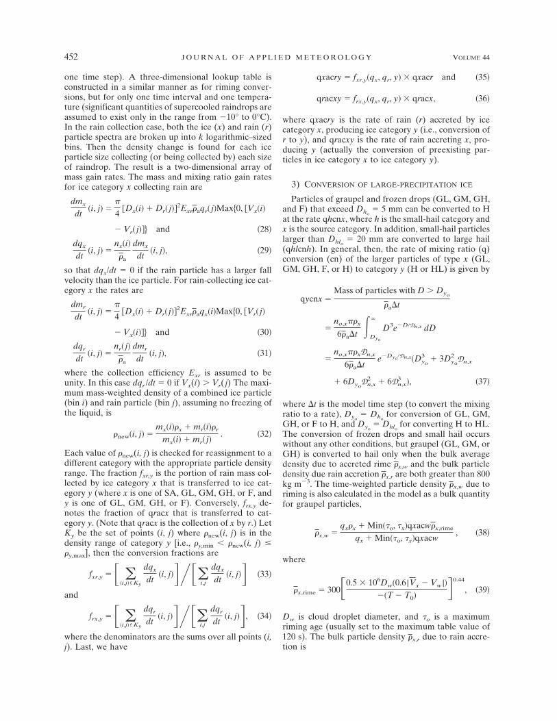
one time step). A three-dimensional lookup table isconstructed in a similar manner as for riming conver-sions, but for only one time interval and one tempera-ture (significant quantities of supercooled raindrops areassumed to exist only in the range from �10° to 0°C).In the rain collection case, both the ice (x) and rain (r)particle spectra are broken up into k logarithmic–sizedbins. Then the density change is found for each iceparticle size collecting (or being collected by) each sizeof raindrop. The result is a two-dimensional array ofmass gain rates. The mass and mixing ratio gain ratesfor ice category x collecting rain are

dmx

dt�i, j� �

�

4�Dx�i� � Dr� j��2Exr�aqr� j�Max�0, �Vx�i�

� Vr� j�� and �28�

dqx

dt�i, j� �

nx�i�

�a

dmx

dt�i, j�, �29�

so that dqx/dt � 0 if the rain particle has a larger fallvelocity than the ice particle. For rain-collecting ice cat-egory x the rates are

dmr

dt�i, j� �

�

4�Dx�i� � Dr� j��2Exr�aqx�i�Max�0, �Vr� j�

� Vx�i�� and �30�

dqr

dt�i, j� �

nr� j�

�a

dmr

dt�i, j�, �31�

where the collection efficiency Exr is assumed to beunity. In this case dqr /dt � 0 if Vx(i) � Vr( j) The maxi-mum mass-weighted density of a combined ice particle(bin i) and rain particle (bin j), assuming no freezing ofthe liquid, is

�new�i, j� �mx�i��x � mr�i��r

mx�i� � mr� j�. �32�

Each value of �new(i, j) is checked for reassignment to adifferent category with the appropriate particle densityrange. The fraction fxr,y is the portion of rain mass col-lected by ice category x that is transferred to ice cat-egory y (where x is one of SA, GL, GM, GH, or F, andy is one of GL, GM, GH, or F). Conversely, frx,y de-notes the fraction of qracx that is transferred to cat-egory y. (Note that qracx is the collection of x by r.) LetKy be the set of points (i, j) where �new(i, j) is in thedensity range of category y [i.e., �y,min �new(i, j) ��y,max], then the conversion fractions are

fxr,y � � ��i,j��Ky

dqx

dt�i, j��

i,j

dqx

dt�i, j�� 33�

and

frx,y � � ��i,j��Ky

dqr

dt�i, j��

i,j

dqr

dt�i, j��, �34�

where the denominators are the sums over all points (i,j). Last, we have

qxacry � fxr,y�qx, qr, y� qxacr and �35�

qracxy � frx,y�qx, qr, y� qracx, �36�

where qxacry is the rate of rain (r) accreted by icecategory x, producing ice category y (i.e., conversion ofr to y), and qracxy is the rate of rain accreting x, pro-ducing y (actually the conversion of preexisting par-ticles in ice category x to ice category y).

3) CONVERSION OF LARGE-PRECIPITATION ICE

Particles of graupel and frozen drops (GL, GM, GH,and F) that exceed Dho

� 5 mm can be converted to Hat the rate qhcnx, where h is the small-hail category andx is the source category. In addition, small-hail particleslarger than Dhlo

� 20 mm are converted to large hail(qhlcnh). In general, then, the rate of mixing ratio (q)conversion (cn) of the larger particles of type x (GL,GM, GH, F, or H) to category y (H or HL) is given by

qycnx �Mass of particles with D Dyo

�a�t

�no,x��x

6�a�t Dyo

�

D3e�D�Dn,x dD

�no,x��xDn,x

6�a�te�Dyo�Dn,x�Dyo

3 � 3Dyo

2 Dn,x

� 6DyoDn,x

2 � 6Dn,x3 �, �37�

where �t is the model time step (to convert the mixingratio to a rate), Dyo

� Dhofor conversion of GL, GM,

GH, or F to H, and Dyo� Dhlo

for converting H to HL.The conversion of frozen drops and small hail occurswithout any other conditions, but graupel (GL, GM, orGH) is converted to hail only when the bulk averagedensity due to accreted rime �x,w and the bulk particledensity due rain accretion �x,r are both greater than 800kg m�3. The time-weighted particle density �x,w due toriming is also calculated in the model as a bulk quantityfor graupel particles,

�x,w �qx�x � Min��o, �x�qxacw�x,rime

qx � Min��o, �x�qxacw, �38�

where

�x,rime � 300�0.5 106Dw�0.6 |Vx � Vw |��T � T0�

�0.44

, �39�

Dw is cloud droplet diameter, and �o is a maximumriming age (usually set to the maximum table value of120 s). The bulk particle density �x,r due to rain accre-tion is


�*x,r � �qx�x � �t�qxacr��r

qx � �t�qxacr� � and

�x,r � Min�Max��*x,r, 100�, 900�, �40�

where �r is the rain particle density (1000 kg m�3) andqxacr is the rain accretion rate by precipitation ice spe-cies x.

d. Additional processes in 10-ICE

This section describes the additional microphysicalprocesses that are not treated by the 3-ICE schemedescribed by GSR04.

1) ICE CRYSTAL AGGREGATION

The self-collection rate for ice crystal aggregation tosnow is calculated following the Cotton et al. (1986)adaptation of the aggregation model 1 in Passarelli andSrivastava (1979):

qscni � 0.25��a

6miEiiqi

2Di2Vi, �41�

where mi is the ice crystal mass, Di is the crystal diam-eter (or, for rimed ice, the characteristic diameter Dn,ir),and Vi is the terminal fall velocity. [Note that qscni �production of snow (s) by conversion (cn) of ice crystals(i).] The ice–ice collection efficiency is Eii � 0.1 exp(0.1Tc). The same equation is applied to ice crystal columnsand plates and to rimed ice. The rates of one ice crystaltype collecting another are treated also as source termsfor snow aggregates. The cross collections are treatedas MD–MD or MD–IE distribution collection equa-tions, as appropriate.

2) INITIATION OF PRECIPITATION BY THE ICEPROCESS

The ice process of precipitation formation beginswith the riming of pristine cloud ice crystals (IP and CI)to become small IR and GL. The accumulated mass ofrime per ice crystal mrime is calculated from the currentcrystal-riming rate (qiacw) and the riming age �i:

mrime ��a�i

niqiacw. �42�

Mass transfers to categories IR and GL are calculatedfrom the mass fraction of rime frime,

frime � Min�1,mrime

mi�, �43�

where mi is the ice crystal (IP or CI) mass. Conversionis initiated when the following two conditions are met:1) frime � 0.1, and 2) the riming rate (qiacw) exceeds thegreater value of 10�12 s�1 and the vapor deposition rateqidp� (10), similar to the approach of Reisner et al.

(1998). The assumption is that the crystals will notchange substantially in character until an appreciablefraction of their mass comes from riming and the rimingmass gain rate is greater than the vapor deposition rate.The portion of newly acquired rime on the crystals thatcan be converted to IR and GL is qiacw0,

qiacw0 � Max�qiacw � qidp, 0�. �44�

As in the graupel conversions, the portion of the pre-existing crystal mixing ratio that is available for conver-sion (qicn0) is determined from the reverse collectionrate qwaci:

qicn0 � Min�qwaci qiacw0qiacw

, 0.1 qi�. �45�

The available rime (qiacw0) and preexisting crystalmixing ratio (qicn0) are partitioned into rimed ice andlow-density graupel. The fraction of each that is con-verted to GL is frime, and the part going to IR is (1 �frime). The continuous shift between IR and GL pro-vided by frime parameterizes the increasingly graupel-like characteristics of heavily rimed crystals. The sameprocedure is also applied to IR for conversion to GL,except that there is only one output category (GL) forthe converted mass, and so there is no need for frime.

3) ICE MULTIPLICATION AND ENHANCEMENT

The model also includes a Hallett–Mossop ice mul-tiplication parameterization (Hallett and Mossop1974). The scheme follows Cotton et al. (1986) (type I,type II) but employs the stair-step temperature func-tion (HMT) of Ferrier (1994) instead of the triangle-shaped function f1(Tp) in Cotton et al. (1986). Both thetype-I (350 splinters formed for every 1 10�3 g ofcloud water accreted) and type-II (one splinter formedfor every 250 cloud droplets larger than 24 �m in di-ameter accreted by graupel or hail) schemes of Cottonet al. (1986) are included. We generally use only thetype-II term because it seems to have more laboratorysupport (Mossop 1976, 1985). The type-II parameter-ization treats the droplet distribution as a gamma func-tion of volume, with a mean diameter being the same asthe monodisperse diameter (Cotton et al. 1986). (Drop-lets are otherwise treated as monodisperse, except forautoconversion.) The mass of the ice splinters has adefault value of 5 10�10 kg. The Hobbs–Rangno iceenhancement parameterization of Ferrier (1994) is alsoincluded (Hobbs and Rangno 1985; Hobbs 1990;Rangno and Hobbs 1991).

4) CLOUD ICE INITIATION

Primary ice initiation follows Meyers et al. (1992)and Ferrier (1994). In addition, contact-freezing nucle-ation of cloud droplets is the same as in Meyers et al.(1992).


5) CLOUD WATER TO RAIN CONVERSION

The autoconversion scheme uses the method ofStraka and Rasmussen (1997) to determine theLagrangian parcel age (15). This Lagrangian informa-tion is then used to delay the conversion of dropletsto rain until a minimum mixing ratio of cloud water(qw,min � 0.01 g kg�1) has existed in the parcel for agiven time �a � �a,o [typically �a,o � 5 to 10 min, and �a

is determined by (16)]. Other than the delay time, theautoconversion of droplets to rain follows Ferrier(1994), which has a modified version of Berry (1968) asadapted by Orville and Kopp (1977). Ferrier (1994)used a minimum droplet size Dw,o to set the thresholdmixing ratio qw,o:

qw,o ��

6nwDw,o

�w

�a,

qdiff � Max�0, �qw � qw,o��, and �46�

qrcnw ��1 10�3�a�qdiff

2

1.2 10�4 �1.596 10�12�1 10�3�nw

��aqdiff

,

�47�

where Dw,o � 20 10�6 m, � is the assumed dropletdispersion (typical value of 0.15–0.3), and

�� 0 for �a � �a,o

1 for �a � �a,o. �48�

The factors of 1 10�3 are included for conversionfrom the SI variable units to the cgs equation units,preserving the original constants.

3. Example results

Two storm environments were used to illustrate thetreatment of the two modes of precipitation formationcommonly referred to as the warm and cold rain pro-cesses. In the warm rain process, raindrops develop bythe collision and coalescence of cloud droplets. Theraindrops may freeze if an updraft carries them abovethe melting level, and the resulting frozen drop maysubsequently be converted by riming into other ice par-ticle types. The cold rain, or ice precipitation, processbegins with the appearance of ice crystals, either by thefreezing of liquid cloud droplets or initiation by vapordeposition onto an ice nucleus. A few of the ice crystalsgrow large enough to start collecting cloud droplets anddevelop into graupel. Graupel particles eventually fallbelow the melting level to become rain. A continentalmulticell storm illustrates the ice process, and the warmrain process is demonstrated in a Florida (maritime)storm simulation. For evaluating model precipitationfields, the estimation of radar reflectivity follows Fer-rier (1994), with the simplifying assumption that all ice

particles are dry. For comparison, the multicell stormwas also simulated with the 3-ICE microphysicalscheme, and results are presented in appendix A.

a. Model numerics and dynamics

The numerical simulation model is nonhydrostaticand fully compressible (Straka 1989; Straka and Ander-son 1993b)and is based on the set of equations de-scribed by Klemp and Wilhelmson (1978). Prognosticequations are included for three momentum compo-nents—pressure, potential temperature, and turbulentkinetic energy (see Carpenter et al. 1998). The advec-tion and diffusion numerics in the model all include aconservation principle. For momentum advection, themodel uses a time-centered, quadratic (i.e., energy)conserving “box” scheme (Kurihara and Holloway1967) in the vertical direction, and a sixth-order localspectral scheme in the horizontal (Straka and Anderson1993a). Scalar advection is performed with a forward-in-time, sixth-order, flux divergence–corrected Crowleyscheme (Tremback et al. 1987) with a monotonic filter(Leonard 1991). The same sixth-order Crowley methodis applied in the vertical direction to treat the hydro-meteor fallout terms, resulting in much less computa-tional smoothing than from a first-order treatment. Theturbulent mixing parameterization is based on Klempand Wilhelmson (1978), Deardorff (1980), and Moeng(1984) (see Carpenter et al. 1998).

b. Continental storm

A continental multicell storm simulation exhibits theice precipitation process in the 10-ICE microphysics.An analytical thermodynamic sounding was used fol-lowing Weisman and Klemp (1982), with a boundarylayer vapor mixing ratio of 13.5 g kg�1, resulting inconvective available potential energy (CAPE) of about1630 J kg�1 and convective inhibition (CIN) of 44 Jkg�1. The environment had a half-circle hodograph(Us � 20 m s�1) with the wind shear confined to thelowest 5 km, as in Weisman and Klemp (1984). Therelative humidity profile H(z) is slightly reduced fromthat of Weisman and Klemp (1982):

H�z� � 1 � �� z

ztr�5�4

for z � ztr

Htr for z ztr

, �49�

where � and Htr have values of 0.9 and 0.1, respectively,and H is limited to a maximum value of 0.9. Weismanand Klemp (1982) used values of � � 0.75 and Htr �0.25. The new humidity profile is slightly drier, and thetop of the moist boundary layer is slightly lower thanfrom the original formulation.

The concentration of cloud condensation nuclei(CCN) was set at 109 m�3, and the droplet dispersion is� � 0.15, consistent with a continental storm. The rainautoconversion time delay �a,0 was set at 5 min. It turns


out, however, that in this case the time delay setting isnot important because the high cloud droplet concen-tration causes the mixing ratio threshold qw,o in (46) tobe high enough to prevent rain autoconversion out-right. The simulation has many of the characteristicstypical of Colorado storms (Dye et al. 1974), which arecharacterized by a precipitation-free updraft base andcloud droplets that are too small for effective growth bycollision–coalescence. The simulated cloud base, how-ever, is more typical of central plains storms (i.e.,lower) than of high plains storms (e.g., Dye et al. 1974).The high prescribed CCN concentration guaranteessmall cloud droplets and effectively turns off autocon-version in the model. All rain originates from the melt-ing of ice particles or shedding from wet collectiongrowth. The results are, therefore, quite different fromthe simulation of Weisman and Klemp (1984) for thesame shear profile. Weisman and Klemp (1984) used awarm rain microphysics scheme that rapidly forms rainvia autoconversion in the updraft, and the rain subse-quently fell back through the updraft base.

The computational domain was 45 km 45 km 17.5 km, with constant horizontal grid spacing of 500 mand vertical spacing of 200 m at the surface, stretchingto a constant 500 m above 8.75 km. Convection wasinitiated with a warm spheroid with a central tempera-ture perturbation of 0.9 K. The spheroid radii were 5km 5 km 1.5 km. Random fluctuations in the rangeof �20% of the local perturbation value were added tothe warm bubble to increase entrainment and mixing inthe initial thermal. The bubble was not moistened, pre-serving the dewpoint temperature. Storm longevity isquite sensitive to the sounding and initial conditions. Atest simulation using an original Weisman and Klemp(1982) profile without limiting H resulted in substan-tially stronger and long-lived convection. Another testfound that an initial bubble with no random perturba-tions also resulted in a somewhat stronger final cell.

1) ICE PRECIPITATION INITIATION PROCESS

The ice process is most easily seen in the initial up-draft cell. Figure 2 shows the evolution of ice crystals,rimed crystals, and low- and medium-density graupel asthe initial cell grows. At 17 min the cloud consists ofcloud droplets and trace amounts of pristine ice crystals(plates and columns added together). By 18–20 min,cloud ice has rimed sufficiently for small amounts ofrimed crystals and graupel to appear. The maximummixing ratio of rimed crystals stays relatively small be-cause the collection of plentiful supercooled clouddroplets tends to convert rimed crystals rapidly intolow-density graupel. Riming is sufficient to convertsome low-density graupel to medium-density graupel,but the low temperature and small droplets prevent anyhigh-density graupel production until later in the stormevolution.

The initial updraft cell contains relatively large mix-

ing ratios (�7 g kg�1) of cloud droplets. The high CCNconcentration results in droplets that are too small (lessthan Dw,o) for effective coalescence, as observed forsome Colorado storms (Dye et al. 1974). By 24 min (notshown), and later in the storm (Fig. 5), over 1 g kg�1 ofsupercooled cloud droplets persists at �35°C. This rela-tively high cloud droplet content is consistent with theobservations of Rosenfeld and Woodley (2000), whofound contents as high as 1.8–4 g m�3 at temperaturesnear �38°C.

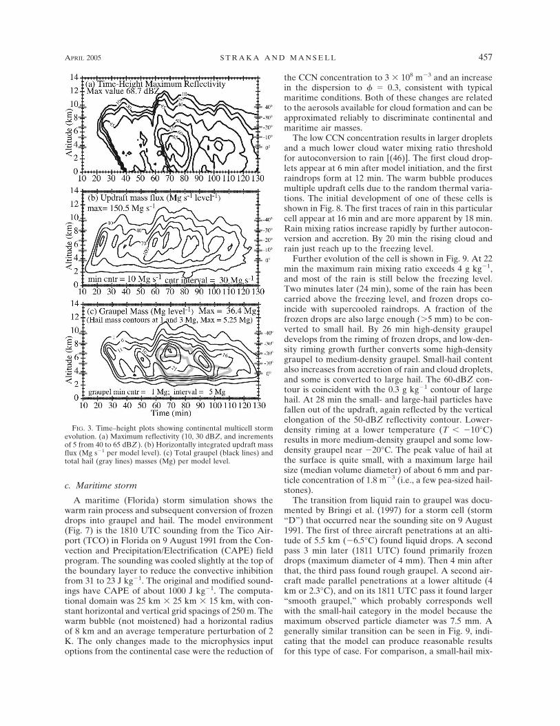
2) MULTICELL EVOLUTION

The continental multicell storm has a series of up-draft pulses (Fig. 3b) at 20, 30, 37, and 52 min that growon the northwestern edge of the storm. Each pulse isconnected to a relatively steady updraft base at 3–4 kmAGL, following the “weak evolution” model of Footeand Frank (1983) based on the Westplains, Colorado,storm. (For comparison, in the “strong evolution”model each updraft has a new base.) At 38 min the thirdcell is an updraft pulse at 4–6 km (Fig. 4). Precipitationfrom the first cell has almost reached the ground, whilethe second cell is decaying. Ice precipitation appears atthe top of cell 3 by 44 min (6–9-km altitude), as themain reflectivity region of cell 2 falls below 7 km. Cell3 reaches maturity by 50 min, and, as in the case studiedby Foote and Frank (1983), the updraft base remainsfree of precipitation (Fig. 4).

The strongest updraft pulse at 52 min is closely fol-lowed by a new updraft (and new updraft base) around62 min. These two updrafts are the first to recycle sig-nificant amounts of graupel and meltwater rain fromthe precipitation shaft back into the updraft, leading toincreases in graupel and the formation of hail (Fig. 3c).The recycling process also results in the appearance ofhigh precipitation content in the updraft (Fig. 5b) be-fore the main cell collapses. A weak left-moving celldevelops by about 80 min (Fig. 5a at 26 km north, 16 kmeast) and dissipates within 15 min.

3) MATURE STAGE

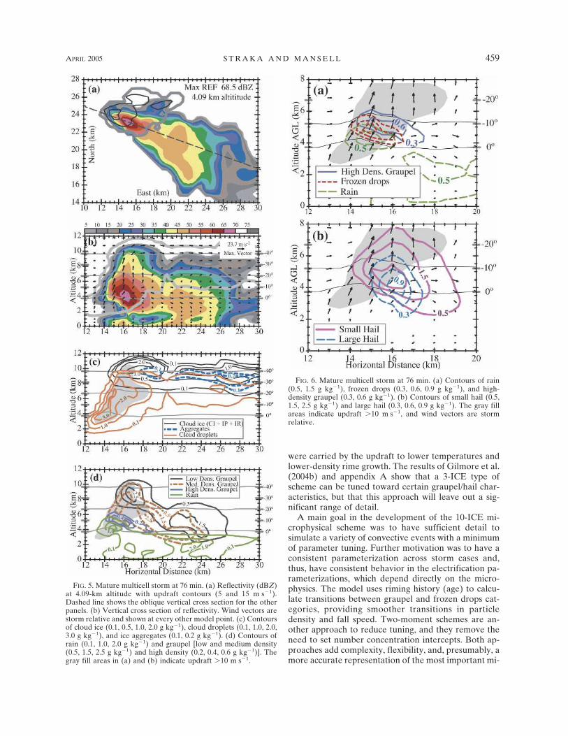
The multicell storm at its mature stage exhibits all ofthe 10-ICE hydrometeor types. Figures 5 and 6 showhydrometeor fields and simulated radar reflectivity at76 min. Cloud ice, aggregates, and cloud droplets areshown in Fig. 5c. The maximum of cloud ice crystalcontent is at the top of the updraft at temperatures lessthan �40°C, where the cloud droplets freeze homoge-neously. The relatively small mixing ratios of aggre-gates indicate that the mechanism is not very active atthe low temperatures (T �30°C) where ice crystalsare plentiful but collection and sticking/interlocking ef-ficiencies are low. Low- and medium-density graupelcan be seen precipitating out of the storm and meltinginto rain (Fig. 5b). The lower fall velocity of low-densitygraupel allows it to be carried farther downstream than


the medium-density graupel, resulting in an elongatedregion of precipitation. Rimed ice crystals have ratherlow mixing ratios (on the order of 10�5 kg kg�1) and arenot shown, but they have a maximum content in thelower half of the anvil where ice crystals and super-cooled drops coexist.

The updraft region up to 8 km is shown in greaterdetail in Fig. 6 (also at 76 min). As suggested by Fig. 5b,meltwater rain is being recycled into the updraft andcarried above the freezing level, resulting in frozen

drops. Some rain may also appear from shedding fromhail or high-density graupel, but the rain at the updraftbase (0°C) in Fig. 6a started as meltwater that increasedin content via cloud droplet collection. High-densitygraupel is mainly confined to the updraft core, where itforms from the riming of frozen drops (Fig. 6a) andmedium-density graupel. Small hail has appeared as theresult of the conversion of the larger graupel and frozendrop particles, and large hail comes from conversion ofthe upper end of the small hail spectrum (Fig. 6b).

FIG. 2. Development of ice precipitation in an initial updraft. Ice crystals appear first after cloud water, thenrimed ice, then low- and medium-density graupel. All contour units are grams per kilogram. The gray-filled areasindicate updraft �10 m s�1. Values given are for minimum contour level (“min”), contour interval (“intvl”), andmaximum value in the contour plane (“max”). There is no rain at these times. See text for more details.


c. Maritime storm

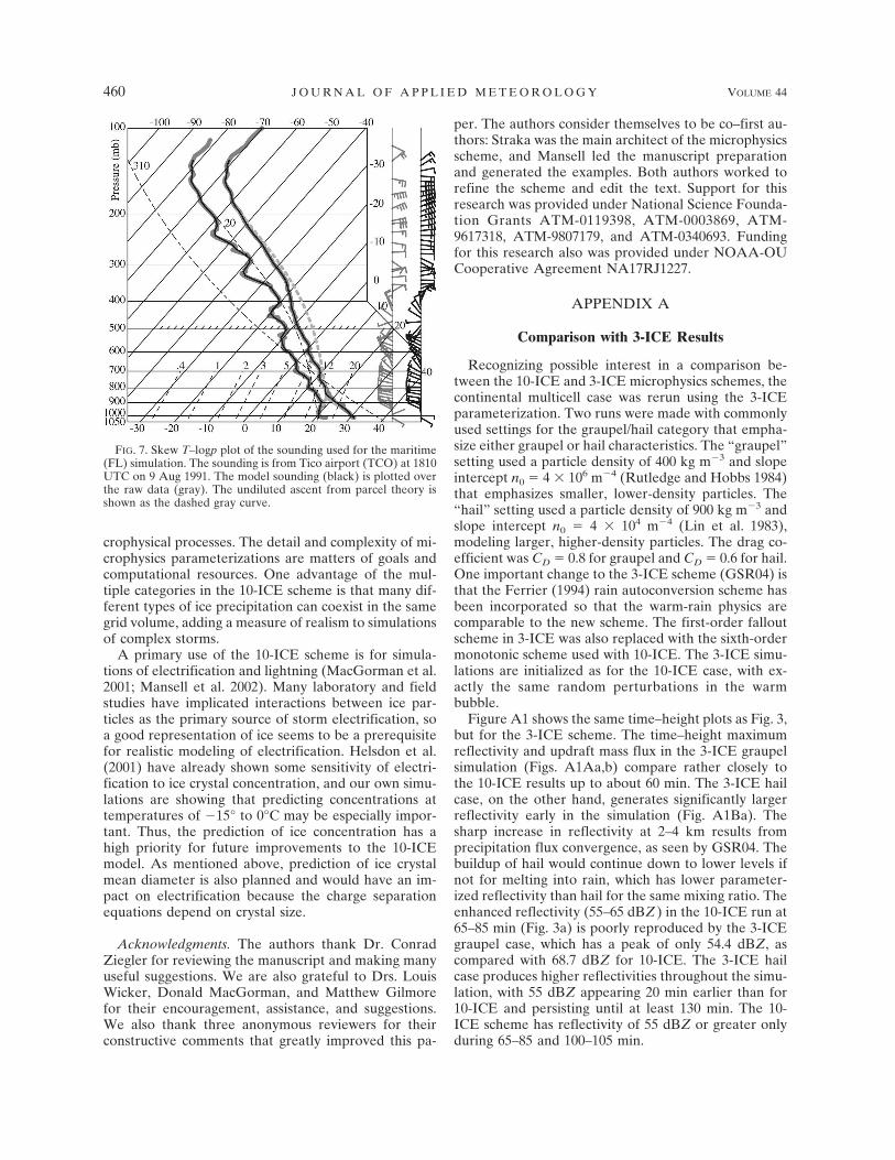
A maritime (Florida) storm simulation shows thewarm rain process and subsequent conversion of frozendrops into graupel and hail. The model environment(Fig. 7) is the 1810 UTC sounding from the Tico Air-port (TCO) in Florida on 9 August 1991 from the Con-vection and Precipitation/Electrification (CAPE) fieldprogram. The sounding was cooled slightly at the top ofthe boundary layer to reduce the convective inhibitionfrom 31 to 23 J kg�1. The original and modified sound-ings have CAPE of about 1000 J kg�1. The computa-tional domain was 25 km 25 km 15 km, with con-stant horizontal and vertical grid spacings of 250 m. Thewarm bubble (not moistened) had a horizontal radiusof 8 km and an average temperature perturbation of 2K. The only changes made to the microphysics inputoptions from the continental case were the reduction of

the CCN concentration to 3 108 m�3 and an increasein the dispersion to � � 0.3, consistent with typicalmaritime conditions. Both of these changes are relatedto the aerosols available for cloud formation and can beapproximated reliably to discriminate continental andmaritime air masses.

The low CCN concentration results in larger dropletsand a much lower cloud water mixing ratio thresholdfor autoconversion to rain [(46)]. The first cloud drop-lets appear at 6 min after model initiation, and the firstraindrops form at 12 min. The warm bubble producesmultiple updraft cells due to the random thermal varia-tions. The initial development of one of these cells isshown in Fig. 8. The first traces of rain in this particularcell appear at 16 min and are more apparent by 18 min.Rain mixing ratios increase rapidly by further autocon-version and accretion. By 20 min the rising cloud andrain just reach up to the freezing level.

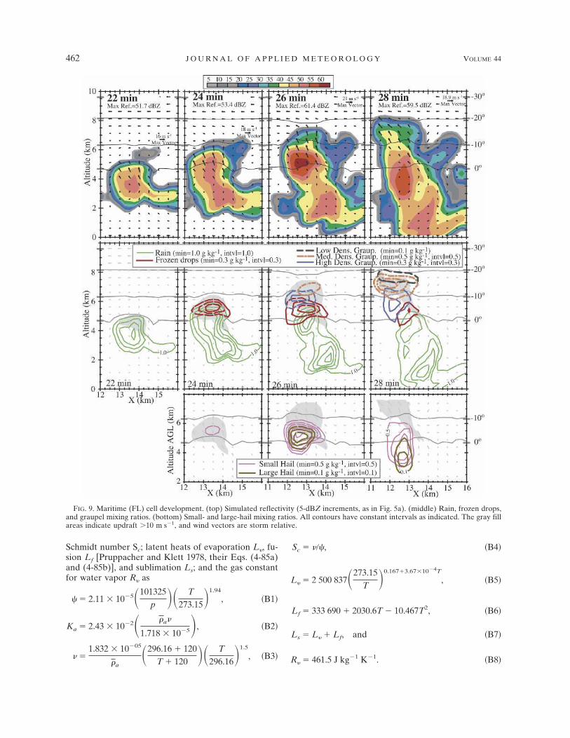
Further evolution of the cell is shown in Fig. 9. At 22min the maximum rain mixing ratio exceeds 4 g kg�1,and most of the rain is still below the freezing level.Two minutes later (24 min), some of the rain has beencarried above the freezing level, and frozen drops co-incide with supercooled raindrops. A fraction of thefrozen drops are also large enough (�5 mm) to be con-verted to small hail. By 26 min high-density graupeldevelops from the riming of frozen drops, and low-den-sity riming growth further converts some high-densitygraupel to medium-density graupel. Small-hail contentalso increases from accretion of rain and cloud droplets,and some is converted to large hail. The 60-dBZ con-tour is coincident with the 0.3 g kg�1 contour of largehail. At 28 min the small- and large-hail particles havefallen out of the updraft, again reflected by the verticalelongation of the 50-dBZ reflectivity contour. Lower-density riming at a lower temperature (T �10°C)results in more medium-density graupel and some low-density graupel near �20°C. The peak value of hail atthe surface is quite small, with a maximum large hailsize (median volume diameter) of about 6 mm and par-ticle concentration of 1.8 m�3 (i.e., a few pea-sized hail-stones).

The transition from liquid rain to graupel was docu-mented by Bringi et al. (1997) for a storm cell (storm“D”) that occurred near the sounding site on 9 August1991. The first of three aircraft penetrations at an alti-tude of 5.5 km (�6.5°C) found liquid drops. A secondpass 3 min later (1811 UTC) found primarily frozendrops (maximum diameter of 4 mm). Then 4 min afterthat, the third pass found rough graupel. A second air-craft made parallel penetrations at a lower altitude (4km or 2.3°C), and on its 1811 UTC pass it found larger“smooth graupel,” which probably corresponds wellwith the small-hail category in the model because themaximum observed particle diameter was 7.5 mm. Agenerally similar transition can be seen in Fig. 9, indi-cating that the model can produce reasonable resultsfor this type of case. For comparison, a small-hail mix-

FIG. 3. Time–height plots showing continental multicell stormevolution. (a) Maximum reflectivity (10, 30 dBZ, and incrementsof 5 from 40 to 65 dBZ ). (b) Horizontally integrated updraft massflux (Mg s�1 per model level). (c) Total graupel (black lines) andtotal hail (gray lines) masses (Mg) per model level.


ing ratio of 3 g kg�1 at 4-km altitude gives a medianvolume diameter (D�) of about 8 mm and a total con-centration of 90 m�3. Large hail of 0.3 g kg�1 at thesame altitude would have D� � 11 mm but a concen-tration of only 3 m�3.

4. Discussion and conclusions

The test simulations exhibit some of the reasonableresults obtainable with the 10-ICE scheme for stormsdominated by different precipitation processes. The

continental storm first developed low- and medium-density graupel, and eventually high-density graupeland hail appeared in the storm core. The precipitationdistribution at the ground also is strongly influenced byhorizontal distribution of ice particles. The storm, ingeneral, follows the “weak” multicell evolution modelof Foote and Frank (1983). In the maritime storm, onthe other hand, the first large ice particles were frozendrops, which quickly converted to both small hail andhigh-density graupel. The high-density graupel con-verted to medium- and low-density graupel as particles

FIG. 4. Growth of the third updraft cell in the multicell storm. The cloud boundary is denoted by the heavy grayline. Reflectivity contours (gray fill) have values of 10, 20, 30, and 40 dBZ. (right) The horizontal cross sections aretaken at 4.09-km altitude, where the thin black contours show updraft speeds of 5 and 15 m s�1. The dashed lineindicates the plane of the corresponding vertical cross section shown on the left. Note that the horizontal axis along(left) the vertical sections indicates the distance along the oblique from the western edge of the domain.


were carried by the updraft to lower temperatures andlower-density rime growth. The results of Gilmore et al.(2004b) and appendix A show that a 3-ICE type ofscheme can be tuned toward certain graupel/hail char-acteristics, but that this approach will leave out a sig-nificant range of detail.

A main goal in the development of the 10-ICE mi-crophysical scheme was to have sufficient detail tosimulate a variety of convective events with a minimumof parameter tuning. Further motivation was to have aconsistent parameterization across storm cases and,thus, have consistent behavior in the electrification pa-rameterizations, which depend directly on the micro-physics. The model uses riming history (age) to calcu-late transitions between graupel and frozen drops cat-egories, providing smoother transitions in particledensity and fall speed. Two-moment schemes are an-other approach to reduce tuning, and they remove theneed to set number concentration intercepts. Both ap-proaches add complexity, flexibility, and, presumably, amore accurate representation of the most important mi-

FIG. 5. Mature multicell storm at 76 min. (a) Reflectivity (dBZ)at 4.09-km altitude with updraft contours (5 and 15 m s�1).Dashed line shows the oblique vertical cross section for the otherpanels. (b) Vertical cross section of reflectivity. Wind vectors arestorm relative and shown at every other model point. (c) Contoursof cloud ice (0.1, 0.5, 1.0, 2.0 g kg�1), cloud droplets (0.1, 1.0, 2.0,3.0 g kg�1), and ice aggregates (0.1, 0.2 g kg�1). (d) Contours ofrain (0.1, 1.0, 2.0 g kg�1) and graupel [low and medium density(0.5, 1.5, 2.5 g kg�1) and high density (0.2, 0.4, 0.6 g kg�1)]. Thegray fill areas in (a) and (b) indicate updraft �10 m s�1.

FIG. 6. Mature multicell storm at 76 min. (a) Contours of rain(0.5, 1.5 g kg�1), frozen drops (0.3, 0.6, 0.9 g kg�1), and high-density graupel (0.3, 0.6 g kg�1). (b) Contours of small hail (0.5,1.5, 2.5 g kg�1) and large hail (0.3, 0.6, 0.9 g kg�1). The gray fillareas indicate updraft �10 m s�1, and wind vectors are stormrelative.


Fig 5 6 live 4/C

crophysical processes. The detail and complexity of mi-crophysics parameterizations are matters of goals andcomputational resources. One advantage of the mul-tiple categories in the 10-ICE scheme is that many dif-ferent types of ice precipitation can coexist in the samegrid volume, adding a measure of realism to simulationsof complex storms.

A primary use of the 10-ICE scheme is for simula-tions of electrification and lightning (MacGorman et al.2001; Mansell et al. 2002). Many laboratory and fieldstudies have implicated interactions between ice par-ticles as the primary source of storm electrification, soa good representation of ice seems to be a prerequisitefor realistic modeling of electrification. Helsdon et al.(2001) have already shown some sensitivity of electri-fication to ice crystal concentration, and our own simu-lations are showing that predicting concentrations attemperatures of �15° to 0°C may be especially impor-tant. Thus, the prediction of ice concentration has ahigh priority for future improvements to the 10-ICEmodel. As mentioned above, prediction of ice crystalmean diameter is also planned and would have an im-pact on electrification because the charge separationequations depend on crystal size.

Acknowledgments. The authors thank Dr. ConradZiegler for reviewing the manuscript and making manyuseful suggestions. We are also grateful to Drs. LouisWicker, Donald MacGorman, and Matthew Gilmorefor their encouragement, assistance, and suggestions.We also thank three anonymous reviewers for theirconstructive comments that greatly improved this pa-

per. The authors consider themselves to be co–first au-thors: Straka was the main architect of the microphysicsscheme, and Mansell led the manuscript preparationand generated the examples. Both authors worked torefine the scheme and edit the text. Support for thisresearch was provided under National Science Founda-tion Grants ATM-0119398, ATM-0003869, ATM-9617318, ATM-9807179, and ATM-0340693. Fundingfor this research also was provided under NOAA-OUCooperative Agreement NA17RJ1227.

APPENDIX A

Comparison with 3-ICE Results

Recognizing possible interest in a comparison be-tween the 10-ICE and 3-ICE microphysics schemes, thecontinental multicell case was rerun using the 3-ICEparameterization. Two runs were made with commonlyused settings for the graupel/hail category that empha-size either graupel or hail characteristics. The “graupel”setting used a particle density of 400 kg m�3 and slopeintercept n0 � 4 106 m�4 (Rutledge and Hobbs 1984)that emphasizes smaller, lower-density particles. The“hail” setting used a particle density of 900 kg m�3 andslope intercept n0 � 4 104 m�4 (Lin et al. 1983),modeling larger, higher-density particles. The drag co-efficient was CD � 0.8 for graupel and CD � 0.6 for hail.One important change to the 3-ICE scheme (GSR04) isthat the Ferrier (1994) rain autoconversion scheme hasbeen incorporated so that the warm-rain physics arecomparable to the new scheme. The first-order falloutscheme in 3-ICE was also replaced with the sixth-ordermonotonic scheme used with 10-ICE. The 3-ICE simu-lations are initialized as for the 10-ICE case, with ex-actly the same random perturbations in the warmbubble.

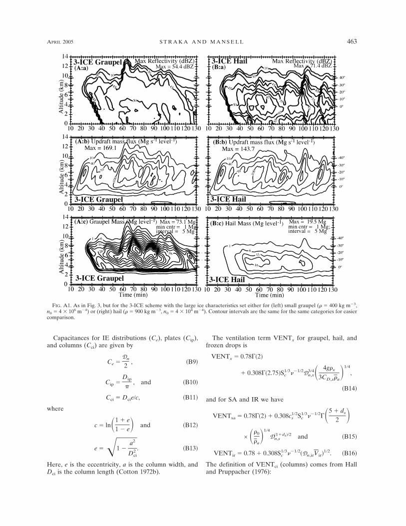
Figure A1 shows the same time–height plots as Fig. 3,but for the 3-ICE scheme. The time–height maximumreflectivity and updraft mass flux in the 3-ICE graupelsimulation (Figs. A1Aa,b) compare rather closely tothe 10-ICE results up to about 60 min. The 3-ICE hailcase, on the other hand, generates significantly largerreflectivity early in the simulation (Fig. A1Ba). Thesharp increase in reflectivity at 2–4 km results fromprecipitation flux convergence, as seen by GSR04. Thebuildup of hail would continue down to lower levels ifnot for melting into rain, which has lower parameter-ized reflectivity than hail for the same mixing ratio. Theenhanced reflectivity (55–65 dBZ) in the 10-ICE run at65–85 min (Fig. 3a) is poorly reproduced by the 3-ICEgraupel case, which has a peak of only 54.4 dBZ, ascompared with 68.7 dBZ for 10-ICE. The 3-ICE hailcase produces higher reflectivities throughout the simu-lation, with 55 dBZ appearing 20 min earlier than for10-ICE and persisting until at least 130 min. The 10-ICE scheme has reflectivity of 55 dBZ or greater onlyduring 65–85 and 100–105 min.

FIG. 7. Skew T–logp plot of the sounding used for the maritime(FL) simulation. The sounding is from Tico airport (TCO) at 1810UTC on 9 Aug 1991. The model sounding (black) is plotted overthe raw data (gray). The undiluted ascent from parcel theory isshown as the dashed gray curve.


The 3-ICE graupel case has much more mass in thegraupel/hail field than the hail case (Figs. A1Ac,A1Bc). Conversely, the 3-ICE hail case has much moremass in the snowfield (not shown) than 3-ICE graupel.The main cause is the difference between the cloudwater collection rate of graupel versus hail (Gilmore etal. 2004b). The larger concentrations of graupel athigher altitudes lead to higher cloud water accretion,leaving less cloud water for snow to collect. Althoughthe graupel has a lower fall speed and accretion ratethan hail, this is compensated by a longer time aloft.Gilmore et al. (2004b) show that the accretion ratesqhacw and qsacw tend to vary inversely as the graupel/hail category characteristics are varied from large hailto small graupel. A contributing factor is the residenceof graupel at higher altitudes than hail, so that it com-petes more directly with snow for cloud water. Cloudice fields (not shown) are more similar, where the hailcase has slightly higher maximum layer mass than thegraupel case (10 versus 6.4 Mg).

The 3-ICE simulations both have higher reflectivityat upper altitudes (Fig. A2, 7–10 km) than the 10-ICEsimulation (Fig. 4) because of greater conversion ratesof cloud ice to snow. The 3-ICE hail case has signifi-

cantly larger regions of reflectivity greater than 40 dBZthan the 3-ICE graupel and 10-ICE cases. At 44 min,both 3-ICE simulations have deeper reflectivity regionsin the growing cell than the 10-ICE case. Significantprecipitation recycling begins sooner in the 3-ICE simu-lations, as indicated at 44 min by the 10-dBZ reflectivitycontour at or below the 0°C isotherm in the updraftregion (20–22-km horizontal distance).

These results with the 3-ICE scheme indicate thattuning the graupel/hail characteristics causes substan-tial changes in results, as found by Gilmore et al.(2004b). There is no particular setting that can reallyhope to simulate a complex storm that contains a largevariety of ice habits. Extra precipitation categories addmore flexibility, or “dynamic range,” in this regard, togenerate more realistic details.

APPENDIX B

Deposition (Sublimation) Variables

We define first the following variables: diffusivity ofwater vapor � in air; thermal conductivity Ka (Wisner etal. 1972) and kinematic viscosity of air (List 1984); the

FIG. 8. Maritime (FL) warm rain process evolution in time. Contours of cloud droplet (qw) and rain (qr) mixing ratio show earlyrain development. All contour units are grams per kilogram, and wind vectors are storm relative.


Schmidt number Sc; latent heats of evaporation L�, fu-sion Lf [Pruppacher and Klett 1978, their Eqs. (4-85a)and (4-85b)], and sublimation Ls; and the gas constantfor water vapor R� as

� 2.11 10�5�101325p �� T

273.15�1.94

, �B1�

Ka � 2.43 10�2� �a�

1.718 10�5�, �B2�

� �1.832 10�05

�a�296.16 � 120

T � 120 �� T

296.16�1.5

, �B3�

Sc � ��, �B4�

L � 2 500 837�273.15T �0.167�3.6710�4T

, �B5�

Lf � 333 690 � 2030.6T � 10.467T2, �B6�

Ls � L � Lf, and �B7�

R � 461.5 J kg�1 K�1. �B8�

FIG. 9. Maritime (FL) cell development. (top) Simulated reflectivity (5-dBZ increments, as in Fig. 5a). (middle) Rain, frozen drops,and graupel mixing ratios. (bottom) Small- and large-hail mixing ratios. All contours have constant intervals as indicated. The gray fillareas indicate updraft �10 m s�1, and wind vectors are storm relative.


Fig 9 live 4/C

Capacitances for IE distributions (Ce), plates (Cip),and columns (Cci) are given by

Ce �Dn

2, �B9�

Cip �Dip

�, and �B10�

Cci � Dcie�c, �B11�

where

c � ln�1 � e

1 � e� and �B12�

e ��1 �a2

Dci2 . �B13�

Here, e is the eccentricity, a is the column width, andDci is the column length (Cotton 1972b).

The ventilation term VENTx for graupel, hail, andfrozen drops is

VENTx � 0.78��2�

� 0.308��2.75�Sc1�3��1�2Dn,x

3�4� 4g�x

3CD,x�a�1�4

,

�B14�

and for SA and IR we have

VENTsa � 0.78��2� � 0.308cs1�2Sc

1�3��1�2��5 � ds

2 �× ��0

�a�1�4

Dn,s�1�ds��2 and �B15�

VENTir � 0.78 � 0.308Sc1�3��1�2�Dn,irVir�

1�2. �B16�

The definition of VENTci (columns) comes from Halland Pruppacher (1976):

FIG. A1. As in Fig. 3, but for the 3-ICE scheme with the large ice characteristics set either for (left) small graupel (� � 400 kg m�3,n0 � 4 106 m�4) or (right) hail (� � 900 kg m�3, n0 � 4 104 m�4). Contour intervals are the same for the same categories for easiercomparison.


VENTci �

�1 � 0.14X2 for X � Sc1�3 Reci

1�2 � 1

0.86 � 0.28X for X � 1,

�B17�

�B18�

and VENTip (plates) comes from Thorpe and Mason(1966):

VENTip � 0.65 � 0.44Sc1�3 Reip

1�2, �B19�

where the Reynolds numbers for columns and platesare (Davis and Auer 1974, converted to SI units)

Reci �1.258 104Dci

2.331 � 5.662 104Dci2.373

��0.8241Dci�0.042 � 1.70�

�B20�

and

Reip �1�

�58.25Dip1.824 � 0.1652Dip

1.299�. �B21�

REFERENCES

Bailey, M., and J. Hallett, 2002: Nucleation effects on the habit ofvapour grown ice crystals from �18 to �42°C. Quart. J. Roy.Meteor. Soc., 128, 1461–1483.

FIG. A2. As for the vertical cross sections in Fig. 4 but for the 3-ICE scheme with settings for (left) small graupel (� � 400 kg m�3,n0 � 4 106 m�4) or (right) hail (� � 900 kg m�3, n0 � 4 104 m�4). Reflectivity contours (gray fill) have values of 10, 20, 30, and40 dBZ.


Berry, E. X., 1967: Cloud droplet growth by collection. J. Atmos.Sci., 24, 688–701.

——, 1968: Modification of the warm rain process. Preprints, FirstNational Conf. on Weather Modification, Albany, NY, Amer.Meteor. Soc., 81–88.

Bigg, E. K., 1953: The supercooling of water. Proc. Phys. Soc.London, B66, 688–694.

Braham, R. R., 1968: Meteorological bases for precipitation de-velopment. Bull. Amer. Meteor. Soc., 49, 343–353.

Bringi, V. N., K. Knupp, A. Detwiler, I. J. Caylor, and R. A.Black, 1997: Evolution of a Florida thunderstorm during theConvection and Precipitation/Electrification Experiment:The case of 9 August 1991. Mon. Wea. Rev., 125, 2131–2160.

Carpenter, R. L., K. K. Droegemeier, and A. M. Blyth, 1998:Entrainment and detrainment in numerically simulated cu-mulus congestus clouds. Part I: General results. J. Atmos.Sci., 55, 3417–3432.

Clark, T., 1974: A study in cloud phase parameterization using thegamma distribution. J. Atmos. Sci., 31, 142–155.

——, 1976: Use of log-normal distributions for numerical calcu-lations of condensation and collection. J. Atmos. Sci., 33, 810–821.

Cotton, W. R., 1972a: Numerical simulation of precipitation de-velopment in supercooled cumuli–Part I. Mon. Wea. Rev.,100, 757–763.

——, 1972b: Numerical simulation of precipitation developmentin supercooled cumuli–Part II. Mon. Wea. Rev., 100, 764–784.

——, M. A. Stephens, T. Nehrkorn, and G. J. Tripoli, 1982: TheColorado State University three-dimensional cloud/meso-scale model–1982. Part II: An ice phase parameterization. J.Rech. Atmos., 16, 295–320.

——, G. J. Tripoli, R. M. Rauber, and E. A. Mulvihill, 1986:Numerical simulation of the effects of varying ice crystalnucleation rates and aggregation processes on orographicsnowfall. J. Climate Appl. Meteor., 25, 1658–1680.

Davis, C. I., and A. H. Auer Jr., 1974: Use of isolated orographicclouds to establish the accuracy of diffusional ice crystalgrowth equations. Preprints, Conf. on Cloud Physics, Tucson,AZ, Amer. Meteor. Soc., 141–147.

Deardorff, J. W., 1980: Stratocumulus-capped mixed layers de-rived from a three-dimensional model. Bound.-Layer Me-teor., 18, 495–527.

Dye, J. E., C. A. Knight, V. Toutenhoofd, and T. W. Cannon,1974: The mechanism of precipitation formation in northeast-ern Colorado cumulus. III. Coordinated microphysical andradar observations and summary. J. Atmos. Sci., 31, 2152–2159.

Farley, R. D., 1987: Numerical modeling of hailstorms and hail-stone growth. Part II: The role of low-density riming growthin hail production. J. Climate Appl. Meteor., 26, 234–254.

Feingold, G., and Z. Levin, 1986: The lognormal fit to raindropspectra from frontal convective clouds in Israel. J. ClimateAppl. Meteor., 25, 1346–1364.

——, R. L. Walko, B. Stevens, and W. R. Cotton, 1998: Simula-tions of marine stratocumulus using a new microphysical pa-rameterization scheme. Atmos. Res., 47–48, 505–528.

Ferrier, B. S., 1994: A double-moment multiple-phase four-classbulk ice scheme. Part I: Description. J. Atmos. Sci., 51, 249–280.

——, W.-K. Tao, and J. Simpson, 1995: A double-moment mul-tiple-phase four-class bulk ice scheme. Part II: Simulations ofconvective storms in different large-scale environments andcomparisons with other bulk parameterizations. J. Atmos.Sci., 52, 1001–1033.

Fletcher, N. H., 1962: The Physics of Rain Clouds. CambridgeUniversity Press, 390 pp.

Foote, G. B., and H. W. Frank, 1983: Case study of a hailstorm inColorado. Part III: Airflow from triple-Doppler measure-ments. J. Atmos. Sci., 40, 686–707.

Gilmore, M. S., J. M. Straka, and E. N. Rasmussen, 2004a: Pre-

cipitation and evolution sensitivity in simulated deep convec-tive storms: Comparisons between liquid-only and simple iceand liquid phase microphysics. Mon. Wea. Rev., 132, 1897–1916.

——, ——, and ——, 2004b: Precipitation uncertainty due tovariations in precipitation particle parameters within a simplemicrophysics scheme. Mon. Wea. Rev., 132, 2610–2627.

Hall, W. D., and H. R. Pruppacher, 1976: The survival of iceparticles falling from cirrus clouds in subsaturated air. J. At-mos. Sci., 33, 1995–2006.

Hallett, J., and S. C. Mossop, 1974: Production of secondary iceparticles during the riming process. Nature, 249, 26–28.

Helsdon, J. H., Jr., and R. D. Farley, 1987: A numerical modelingstudy of a Montana thunderstorm: 2. Model results versusobservations involving electrical aspects. J. Geophys. Res., 92,5661–5675.

——, W. A. Wojcik, and R. D. Farley, 2001: An examination ofthunderstorm-charging mechanisms using a two-dimensionalstorm electrification model. J. Geophys. Res., 106, 1165–1192.

Heymsfield, A. J., and J. C. Pflaum, 1985: A quantitative assess-ment of the accuracy of techniques for calculating graupelgrowth. J. Atmos. Sci., 42, 2264–2274.

Hobbs, P. V., 1990: Ice in clouds. Proc. Conf. on Cloud Physics,San Francisco, CA, Amer. Meteor. Soc., 600–606.

——, and A. L. Rangno, 1985: Ice particle concentrations inclouds. J. Atmos. Sci., 42, 2523–2549.

Kessler, E., 1969: On the Distribution and Continuity of WaterSubstance in Atmospheric Circulations. Meteor. Monogr., No.32, Amer. Meteor. Soc., 84 pp.

Klemp, J. B., and R. B. Wilhelmson, 1978: Simulations of right-and left-moving storms produced through storm splitting. J.Atmos. Sci., 35, 1097–1110.

Kurihara, Y., and J. L. Holloway Jr., 1967: Numerical integrationof a nine-level global primitive equations model formulatedby the box method. Mon. Wea. Rev., 95, 509–530.

Leonard, B. P., 1991: The ULTIMATE conservative differencescheme applied to unsteady one-dimensional advection.Comput. Methods Appl. Mech. Eng., 88, 17–74.

Lin, Y.-L., R. D. Farley, and H. D. Orville, 1983: Bulk parameter-ization of the snow field in a cloud model. J. Climate Appl.Meteor., 22, 1065–1089.

List, R., 1984: Smithsonian Meteorological Tables. 6th ed. Smith-sonian Institution Press, 527 pp.

Liu, J. Y., and H. D. Orville, 1969: Numerical modeling of pre-cipitation and cloud shadow effects on mountain-induced cu-muli. J. Atmos. Sci., 26, 1283–1298.

Lord, S. J., H. E. Willoughby, and J. M. Piotrowicz, 1984: Role ofa parameterized ice-phase microphysics in an axisymmetric,nonhydrostatic tropical cyclone model. J. Atmos. Sci., 41,2836–2848.

MacGorman, D. R., and W. D. Rust, 1998: The Electrical Natureof Storms. Oxford University Press, 422 pp.

——, J. M. Straka, and C. L. Ziegler, 2001: A lightning param-eterization for numerical cloud models. J. Appl. Meteor., 40,459–478.

Macklin, W. C., 1962: The density and structure of ice formed byaccretion. Quart. J. Roy. Meteor. Soc., 88, 30–50.

Mansell, E. R., D. R. MacGorman, C. L. Ziegler, and J. M. Straka,2002: Simulated three-dimensional branched lightning in anumerical thunderstorm model. J. Geophys. Res., 107, 4075,doi:10.1029/2000JD000244.

Mason, B. J., 1971: The Physics of Clouds. Clarendon Press, 670pp.

Meyers, M. P., P. J. DeMott, and W. R. Cotton, 1992: New pri-mary ice-nucleation parameterizations in an explicit cloudmodel. J. Appl. Meteor., 31, 708–721.

——, R. L. Walko, J. Y. Harrington, and W. R. Cotton, 1997: NewRAMS cloud microphysics parameterization. Part II: Thetwo-moment scheme. Atmos. Res., 45, 3–39.

Moeng, C.-H., 1984: A large-eddy-simulation model for the study


of planetary boundary-layer turbulence. J. Atmos. Sci., 41,2052–2062.

Mossop, S. C., 1976: Production of secondary ice particles duringthe growth of graupel by riming. Quart. J. Roy. Meteor. Soc.,102, 25–44.

——, 1985: Secondary ice particle production during rime growth:The effect of drop size distribution and rimer velocity. Quart.J. Roy. Meteor. Soc., 111, 1113–1124.

Ogura, Y., and T. Takahashi, 1973: The development of warm rainin a cumulus model. J. Atmos. Sci., 30, 262–277.

Orville, H. D., and F. J. Kopp, 1977: Numerical simulation of thelife history of a hailstorm. J. Atmos. Sci., 34, 1596–1618.

Passarelli, R. E., and R. C. Srivastava, 1979: A new aspect ofsnowflake aggregation theory. J. Atmos. Sci., 36, 484–493.

Potter, B. E., 1991: Improvements to a commonly used cloudmicrophysical bulk parameterization. J. Appl. Meteor., 30,1040–1042.

Pruppacher, H. R., and J. D. Klett, 1978: Microphysics of Cloudsand Precipitation. Reidel, 774 pp.

Rangno, A. L., and P. V. Hobbs, 1991: Ice particle concentrationsand precipitation development in small polar maritime cu-muliform clouds. Quart. J. Roy. Meteor. Soc., 117, 207–241.

Rasmussen, R. M., and A. J. Heymsfield, 1985: A generalizedform for impact velocities used to determine graupel accre-tional densities. J. Atmos. Sci., 42, 2275–2279.

Reisner, J., R. M. Rasmussen, and R. T. Bruintjes, 1998: Explicitforcasting of supercooled liquid water in winter storms usingthe MM5 mesoscale model. Quart. J. Roy. Meteor. Soc., 124,1071–1107.

Rosenfeld, D., and W. L. Woodley, 2000: Deep convective cloudswith sustained supercooled liquid water down to �37.5°C.Nature, 405, 440–441.

Rutledge, S. A., and P. V. Hobbs, 1984: The mesoscale and mi-croscale structure and organization of clouds and precipita-tion in midlatitude cyclones. XII: A diagnostic modelingstudy of precipitation development in narrow cold-frontalrainbands. J. Atmos. Sci., 41, 2949–2972.

Simpson, J., and V. Wiggert, 1969: Models of precipitating cumu-lus towers. Mon. Wea. Rev., 97, 471–489.

Smith, P. L., 2003: Raindrop size distributions: Exponential or

gamma—Does the difference matter? J. Appl. Meteor., 42,1031–1034.

Straka, J. M., 1989: Hail growth in a highly glaciated central HighPlains multi-cellular hailstorm. Ph.D. thesis, University ofWisconsin—Madison, 413 pp.

——, and J. R. Anderson, 1993a: Extension and application of alocal, minimum aliasing method to multidimensional prob-lems in limited-area domains. Mon. Wea. Rev., 121, 2903–2918.

——, and ——, 1993b: Numerical simulations of microburst-producing storms: Some results from storms observed duringCOHMEX. J. Atmos. Sci., 50, 1329–1348.

——, and E. N. Rasmussen, 1997: Toward improving microphysi-cal parameterizations of conversion processes. J. Appl. Me-teor., 36, 896–902.

——, D. S. Zrnic, and A. V. Ryzhkov, 2000: Bulk hydrometeorclassification and quantifications using polarimetric radardata: Synthesis of relations. J. Appl. Meteor., 39, 1341–1372.

Tao, W.-K., J. Simpson, and M. McCumber, 1989: An ice-watersaturation adjustment. Mon. Wea. Rev., 117, 231–235.

Thorpe, A. D., and B. J. Mason, 1966: The evaporation of icespheres and ice crystals. Brit. J. Appl. Phys., 17, 541–548.

Tremback, C. J., J. Powell, W. R. Cotton, and R. A. Pielke, 1987:The forward-in-time upstream advection scheme: Extensionto higher orders. Mon. Wea. Rev., 115, 540–555.

Verlinde, J., P. J. Flatau, and W. R. Cotton, 1990: Analyticalsolutions to the collection growth equation: Comparison withapproximate methods and application to cloud microphysicsparameterization schemes. J. Atmos. Sci., 47, 2871–2880.

Walko, R. L., W. R. Cotton, M. P. Meyers, and J. Y. Harrington,1995: New RAMS cloud microphysics parameterization. PartI: The single moment scheme. Atmos. Res., 38, 29–62.

Weisman, M. L., and J. B. Klemp, 1982: The dependence of nu-merically simulated convective storms on vertical wind shearand buoyancy. Mon. Wea. Rev., 110, 504–520.

——, and ——, 1984: The structure and classification of numeri-cally simulated convective storms in directionally varyingwind shears. Mon. Wea. Rev., 112, 2479–2498.

Wisner, C., H. D. Orville, and C. Meyers, 1972: A numericalmodel of a hail-bearing cloud. J. Atmos. Sci., 29, 1160–1181.

Ziegler, C. L., 1985: Retrieval of thermal and microphysical vari-ables in observed convective storms. Part I: Model develop-ment and preliminary testing. J. Atmos. Sci., 42, 1487–1509.


Documents

A Bulk Microphysics Parameterization with Multiple Ice ...u0758091/MPschemes/Strakamansell2005.pdf · A Bulk Microphysics Parameterization with Multiple Ice Precipitation Categories