A Brief Introduction to Nonlinear Vibrations

Anindya Chatterjee

Mechanical Engineering, Indian Institute of Science, Bangalore

anindya100@gmail.com

February 2009

I have used these in the past in a lecture given at RCI (Hyderabad), as well as during asummer program at IISc organized by the now-defunct “Nonlinear Studies Group.”

1 General comments

Vibration phenomena that might be modelled well using linear vibration theory include small am-plitude vibrations of long, slender objects like long bridges, aeroplane wings, and helicopter blades;small rocking motions of ships in calm waters; the simplest whirling motions of flexible shafts, and soon. However, interactions between bridges and foundations, between wings/blades and air, betweenships and waves, between shafts and bearings, and so on, are all nonlinear.

Nonlinear systems can display behaviours that linear systems cannot. These include:

(a) multiple steady state solutions, some stable and some unstable, in response to the same inputs,

(b) jump phenomena, involving discontinuous and significant changes in the response of the systemas some forcing parameter is slowly varied,

(c) response at frequencies other than the forcing frequency,

(d) internal resonances, involving different parts of the system vibrating at different frequencies,all with steady amplitudes (the frequencies are usually in rational ratios, such as 1:2, 1:3, 3:5,etc.),

(e) self sustained oscillations in the absence of explicit external periodic forcing, and

(f) complex, irregular motions that are extremely sensitive to initial conditions (chaos).

Analytical intractability and limitations in computational resources make it difficult to system-atically study the abovementioned phenomena in large systems (though harmonic balance is a usefultechnique; see below). For the most part, detailed studies of nonlinear vibrations are conductedusing small systems (with perhaps just one or two degrees of freedom). A good qualitative under-standing of the phenomena observed for the small system is invaluable when the same phenomenaare subsequently encountered in larger systems.

The utility of precise numerical solutions remains high where appropriate. However, in nonlineardynamics it is difficult to extract the qualitative essence from simulations alone. Therefore, anessential complement to all-numerical studies of large nonlinear systems is the analytical/theoreticalstudy of simplified systems.

1

2 Analysis techniques

Three broad categories of techniques for analyzing nonlinear systems are:

(a) heuristic techniques like Galerkin methods, including harmonic balance(b) asymptotic techniques, including the methods of averaging and multiple scales, and(c) rigorous mathematical results about dynamical systems.

This introduction will concentrate on the first two categories.

2.1 Convergent, asymptotic, and heuristic

To make the later discussion more meaningful, let us distinguish between the terms convergent,asymptotic, and heuristic.

A convergent series dependent on a parameter (say, ǫ) is one where if we fix ǫ and take moreand more terms, the sum converges to the correct answer. An asymptotic series dependent on aparameter (say, ǫ “small”) is one where if we take a fixed number of terms and take ǫ smaller andsmaller, the sum gets more and more accurate. Convergent series need not be asymptotic, and viceversa1.

In harmonic balance, there is a periodic solution we wish to approximate. That periodic solutionhas a convergent Fourier series representation. However, in the application of harmonic balance withmany terms, we obtain equally many coupled, usually nonlinear, equations in terms of the coefficients(see below). In practice, harmonic balance is often used with only a few harmonics, usually withexcellent results but never any formal advance guarantees of how accurate the solution will be witha given number of terms included. In this sense, harmonic balance is a heuristic method.

We now discuss these methods in more detail.

2.2 Galerkin methods, and harmonic balance

The basic Galerkin method is now described using a simple boundary value problem,

x + x − 3t = 0 , with x(0) = x(π/2) = 0 .

The exact solution is x = 3t − 3π

2sin t . As an approximation we assume, say, x ≈

N∑

k=1

ak sin 2kt .

Substituting into the governing equation, we obtain a nonzero quantity r(t) called the residual. Wemake r(t) orthogonal to the assumed basis functions, i.e., set

∫ π/2

0

r(t) sin 2kt dt = 0 , for k = 1, 2, · · · , N .

The above process, called a Galerkin projection, yields N equations for the N unknown ak’s, whichupon solution give the approximate solution. The approximation to 3 terms is

x ≈ − sin 2t +1

10sin 4t − 1

35sin 6t ,

which has an error ≤ 0.024. More terms yield more accuracy.

1See, e.g., E. J. Hinch, Perturbation Methods, Cambridge University Press, 1991.

2

Note that for this linear ODE, the equations for the unknown ak’s are linear and algebraic,while for general nonlinear ODE’s these will be nonlinear algebraic equations (see below). Forpartial differential equations in time and space, the approximation will typically be of the formN

∑

k=1

ak(t)φk(x), where the φk are functions of space chosen to suit the problem (e.g., satisfy boundary

conditions).

The technique of Harmonic Balance is a specialized application of the Galerkin method to findperiodic solutions in vibration problems. There are several slightly different versions of the method.Here, we consider unforced, undamped, conservative problems, e.g.,

x + x3 = 0 . (1)

We start with, say, x ≈ A sin ωt + B sin 3ωt . Note that the unknown ω appears in the functionssinωt and sin 3ωt, and so there are actually three unknowns in the two term approximation. Sub-stituting into the differential equation, multiplying in turn by sinωt and sin 3ωt, and integrating ineach case from 0 to 2π/ω and then equating to zero (the Galerkin projection), we obtain:

−Aω2 + 3A3/4 − 3A2B/4 + 3AB2/2 = 0 ,

−9Bω2 − A3/4 + 3A2B/2 + 3B3/4 = 0 .

Treating the indeterminate A as a parameter, we obtain ω = 0.8869A and B = −0.04482A.Variations of the above method are used as the problem changes.Harmonic balance with a few terms usually gives good approximations to periodic solutions. For

example, some numerical results for the above nonlinear oscillations of Eq. 1, as compared with thetwo term harmonic balance calculation given above, are shown in Fig. 1. Oscillations at four differentamplitudes are shown, and the figure appears to have four different curves. Each of these curves isin fact two superimposed and nearly indistinguishable curves (one solid, one dash-dot). The smalldifference between the solid (numerical) and dash-dot (harmonic balance) is visible towards the rightside of the figure (for larger t).

The results show that the two term harmonic balance solution is very accurate. The strongdependence of frequency on amplitude is also clearly seen.

2.3 A first look at asymptotic techniques

Asymptotic techniques depend on some parameter in the problem being very small (or very large,which is the same thing on taking reciprocals). In the limit as the small parameter becomes zero, theproblem should be analytically tractable. The basic ideas can be demonstrated using the followingroot-finding example:

ǫ x6 + x − 1 = 0 , (2)

where 0 < ǫ ≪ 1. If ǫ = 0, x = 1 is the only root. For nonzero ǫ, that root is perturbed to

x = 1 − ǫ + 6ǫ2 − 51ǫ3 + O(ǫ4) .

The O(ǫ4) above represents a quantity that is no bigger than some finite constant times ǫ4, as ǫ goesto zero.

For ǫ 6= 0, Eq. 2 has five other “large” roots, obtainable via a singular perturbation scheme. Oneof them is

x = −ǫ−1/5 − 1

5+

3

25ǫ1/5 − 14

125ǫ2/5 + O(ǫ3/5) .

The two “asymptotic” approximations above are useful for sufficiently small ǫ.

3

0 2 4 6 8 10 12 14 16 18 20−3

−2

−1

0

1

2

3

time

x(t)

Figure 1: Solutions for Eq. 1. Solid line: numerical. Dashdot: harmonic balance (can be viewed asslightly distinct from solid line, for larger times).

2.4 Averaging and multiple scales

The method of averaging is a specialized asymptotic technique for systems of the form

x = ǫf(x, t) , ǫ ≪ 1. (3)

Here, we assume f(x, t) = f(x, t + T ) for all x, t. An approximation to the solution is found bysolving the simpler equation

x = ǫf0(x) , where f0(x) =1

T

∫ T

0

f(x, t) dt .

Nonlinear oscillators, e.g.,x + x = ǫx(1 − x2) , (4)

are not directly amenable to averaging; but they can be put in that form via a change of variables tox = A(t) sin(t+φ(t)) , along with the added constraint equation x = A(t) cos(t+φ(t)) . In this form,the asymptotic method of averaging has been widely used to study a variety of weakly nonlinearoscillators that are slightly perturbed versions of the harmonic oscillator (x + x = 0).

For illustration, Eq. 4 yields the two equations

A = ǫ(

A/2 − A3/8 + A cos(2t + 2φ)/2 + A3 cos(4t + 4φ)/8)

,

φ = ǫ(

− sin(2t + 2φ)/2 + A2 sin(2t + 2φ)/4 − A2 sin(4t + 4φ)/8)

.

4

Finally, by first order averaging (higher order averaging is possible, but not done here), we get

A = ǫ(

A/2 − A3/8)

, and φ = 0 .

The above two equations show that A = 0 is an unstable equilibrium; all other solutions slowly buteventually approach A = 2 (assuming A > 0); and the phase of the oscillation remains steady, atleast at first order.

The method of multiple scales, also applicable to Eq. 3, involves an additional issue, namely theidentification and removal of secular terms, as illustrated below for Eq. 4 using two time scales.

Let t be the actual time; and τ = ǫ t be a slow time. Assume x = x(t, τ). Now

x =∂x

∂t+ ǫ

∂x

∂τ, and x =

∂2x

∂t2+ 2ǫ

∂2x

∂τ∂t+ O(ǫ2) .

Using subscripts t and τ to denote partial derivatives with respect to these quantities, we have

xtt + x = ǫ{

−2xτt + xt

(

1 − x2)}

+ O(ǫ2) .

Assuming a solution of the form x = x0 + ǫx1 + · · ·, we obtain

x0,tt + x0 = ǫ{

−x1,tt − x1 − 2x0,τt + x0,t

(

1 − x2

0

)}

+ O(ǫ2) .

Collecting terms, at leading order we obtain

x0,tt + x0 = 0 ,

which has the general solution x0 = A(τ) sin(t+φ(τ)). Substituting this at the next order we obtain(dropping the explicit dependence of A and φ on τ , and using primes to denote a τ -derivative)

x1,tt + x1 = A3 cos(3t + 3φ)/4 + (−2A′

+ A − A3/4) cos(t + φ) + 2Aφ′

sin(t + φ) .

In the above equation, the solution for x1 can contain t sin(t + φ) and t cos(t + φ) (effectively thesame as t sin t and t cos t). These secular terms make the approximation break down by the timet = O(1/ǫ). The validity of the expansion can be extended by removing the secular terms, whichcan be done here by requiring that the coefficients of the sine and cosine in the forcing be zero, i.e.,−2A

′

+ A − A3/4 = 0 and 2Aφ′

= 0. Noting that A = ǫA′

, etc., we find the evolution of A and φare governed, at this order of approximation, by the same equations as obtained by averaging:

A = ǫ (A/2 − A3/8) , and φ = 0 . (5)

3 The phase plane

Our study of entrainment in section 9 will involve the use of a popular and powerful idea fromnonlinear dynamics: the idea of the phase space. The essential idea is described below.

Consider a system of two equations

x = f(x, y) , and y = g(x, y) .

Sometimes, instead of plotting x and y individually versus t, we just plot x versus y. If, say, x risesmonotonically from 0 to 1 as t increases, while y rises from −1 to 3 during the same time, then on

5

k,c

mx

h

(b)

F(t)k,c

m

x(a)

m

m

1

1

k

k2

2x2

x1

(c)

h

k3

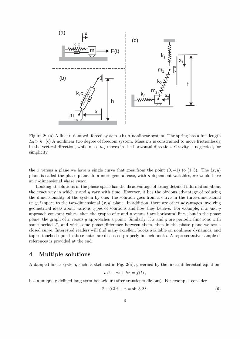
Figure 2: (a) A linear, damped, forced system. (b) A nonlinear system. The spring has a free lengthL0 > h. (c) A nonlinear two degree of freedom system. Mass m1 is constrained to move frictionlesslyin the vertical direction, while mass m2 moves in the horizontal direction. Gravity is neglected, forsimplicity.

the x versus y plane we have a single curve that goes from the point (0,−1) to (1, 3). The (x, y)plane is called the phase plane. In a more general case, with n dependent variables, we would havean n-dimensional phase space.

Looking at solutions in the phase space has the disadvantage of losing detailed information aboutthe exact way in which x and y vary with time. However, it has the obvious advantage of reducingthe dimensionality of the system by one: the solution goes from a curve in the three-dimensional(x, y, t) space to the two-dimensional (x, y) plane. In addition, there are other advantages involvinggeometrical ideas about various types of solutions and how they behave. For example, if x and yapproach constant values, then the graphs of x and y versus t are horizontal lines; but in the phaseplane, the graph of x versus y approaches a point. Similarly, if x and y are periodic functions withsome period T , and with some phase difference between them, then in the phase plane we see aclosed curve. Interested readers will find many excellent books available on nonlinear dynamics, andtopics touched upon in these notes are discussed properly in such books. A representative sample ofreferences is provided at the end.

4 Multiple solutions

A damped linear system, such as sketched in Fig. 2(a), governed by the linear differential equation

mx + cx + kx = f(t) ,

has a uniquely defined long term behaviour (after transients die out). For example, consider

x + 0.3 x + x = sin 3.2 t . (6)

6

0 5 10 15 20 25 30−0.5

−0.4

−0.3

−0.2

−0.1

0

0.1

0.2

0.3

0.4

0.5

time

x(t)

Figure 3: Solutions for Eq. 6 converge to the same long-time behaviour regardless of initial conditions.

Two different solutions, for two different initial conditions, are shown to converge to the same “long-time” solution in Fig. 3.

In contrast, consider the system shown in Fig. 2(b), with the spring’s free length L0 greater thanh. Now it is clear that this nonlinear system will have three equilibrium positions: one at x = 0,which will be unstable, while one stable position at some nonzero positive x, and another (reflected)one for negative x. This simple example shows that it is possible for general deterministic nonlinearsystems to have more than one steady state solution in response to the same inputs (but, of course,with different initial conditions).

This system is not analyzed here in detail; other examples of multiple solutions will soon beanalyzed.

In practical engineering, examples of multiple solutions are encountered in a variety of situations.A few examples are provided below.

• Buckling. Beyond a certain load, the structure has more than one equilibrium; the nominalequilibrium loses stability, and new stable equilibrium positions appear. This is related to thesystem in Fig. 2(b).

• Whirling of shafts at, near and possibly beyond critical speed. A non-whirling solution stillexists, but is now unstable.

• Resonances in nonlinear systems. When the forcing frequency is near the linear natural fre-quency, there can be more than one possible stable steady state solution. This example will becovered again under “jumps”.

7

• Machine tool chatter. Under certain operating conditions, the cutting tool might chatter a lot(poorer surface finish) or very little: there is more than one stable steady state solution.

• Systems with dry friction. Some systems with dry friction, for small forcing near resonance,can have two solutions: one with large amplitude, and one without vibrations.

5 Forced vibrations (via harmonic balance)

Consider the damped nonlinear forced system given by

x + cx + x + ax3 − F sinωt = 0 . (7)

We will study this system using single term harmonic balance. Let us assume x ≈ A sinωt+B cos ωt.The assumption is that the solution is dominated by a response at the same frequency, though notat the same phase, as the forcing. The assumption is exactly true for the linear system (with a = 0),and approximately true for reasonable values of a and most values of ω. This single harmonicapproximation is sufficient for the purposes of this section.

Substituting into the equation of motion and using some trigonometric identities such as sin3 x =(3 sin x − sin 3x)/4, we obtain

−ω2A sinωt − ω2B cos ωt + cωA cos ωt − cωB sinωt + A sin ωt + B cos ωt − 1

4aA3 sin 3ωt

· · · + 3

4aA3 sinωt + 3

4aA2B cos ωt − 3

4aA2B cos 3ωt + 3

4aAB2 sin 3ωt + 3

4aA sinωtB2

· · · + 1

4aB3 cos 3ωt + 3

4aB3 cos ωt − F sinωt = negligible terms.

Multiplying by sinωt or cos ωt, integrating w.r.t. t from 0 to 2π/ω, and then setting them equalto zero, is equivalent to simply picking out the coefficients of sinωt or cos ωt, respectively, and settingthem equal to zero. This gives:

−Aω2 − cBω + A +3

4aA3 +

3

4aAB2 − F = 0 ,

−Bω2 + cAω + B +3

4aA2B +

3

4aB3 = 0 .

The solutions to the two simultaneous equations above provide a fairly accurate picture of thedynamics of the system in Eq. 7.

5.1 Unforced, undamped case

If we put c = 0 and F = 0, then we obtain an approximate solution to the unforced, undampedsystem, for which

B = 0 , and ω =1

2

√

4 + 3aA2 .

The above (approximate) result tells us that for undamped, unforced periodic oscillations the fre-quency of oscillations depends on the amplitude. The graph of A versus ω (i.e., with amplitudealong the vertical axis) is usually called a “backbone curve” because of its shape. In this system,the strength of the nonlinearity is measured by the single quantity a, and so it is not surprisingthat the amplitude dependence of the frequency (which happens only for nonlinear systems) involvesa-dependence as well. It is usual to call the case of a > 0 a stiffening nonlinearity, and the casea < 0 a softening nonlinearity. In the presence of a stiffening nonlinearity, frequency increases withamplitude; in the case of a softening nonlinearity, frequency decreases with amplitude.

8

5.2 Forced, damped case

In the general case, if we select a certain forcing amplitude F and angular frequency ω, then wecan in principle solve for A and B (and hence the response) in terms of a and c. In practice, it isconvenient to solve the equations numerically. Some specific results are shown in the three plots ofFig. 4, where frequency ω is plotted along the horizontal axes and amplitude of response (taken tomean

√A2 + B2 from the harmonic balance equations) is plotted along the vertical axes.

Fig. 4(a) shows the effect of nonlinearity. For a = 0, we have the familiar linear resonance curve.For increasing a while holding all other things constant, the resonance curve leans over to the right(for a stiffening nonlinearity; if we took a < 0 it would lean over to the left).

Fig. 4(b) shows the effect of varying damping c, while holding all other things fixed. Since a isfixed, the backbone curve is fixed. It is seen that the hump in the amplitude versus frequency curvefollows the backbone curve in each case – hence the importance of the backbone curve. All otherthings held fixed, decreasing c raises the hump, i.e., raises the maximum response amplitude possiblewith a given amplitude of harmonic forcing. If we allow both c and F to become very small, theamplitude-frequency curve follows the backbone curve even more closely (not surprising, because thebackbone curve is obtained by setting c = 0, F = 0).

Finally, Fig. 4(c) shows the effect of increasing forcing amplitude while holding other thingsconstant. It is seen that the amplitude versus frequency curve has a hump that leans over to theright; it would lean to the left if the nonlinearity was of the opposite sense, i.e., a was negative. It isseen that for relatively small damping, the hump in the amplitude versus frequency plot follows thebackbone curve. Larger F leads to a higher hump.

A few further remarks may be made about the response of this simple nonlinear system. Forvery high frequencies of forcing, inertia dominates and the amplitude of motion is very small; in suchcases, the x3 nonlinearity is insignificant because |x3| ≪ |x|, and the system behaves essentially likea linear system. The most visible qualitative difference between the linear and nonlinear system is inthe leaning over of the hump near resonance; this is not surprising because large amplitude motionsare (in this system, though not for all systems) the reason for nonlinear terms to become important2.

It is also clear that for F = 2 and ω = 3, say, there are three different possible amplitudes ofresponse (thus, multiple solutions in response to the same input forcing). Of these, it is possible toshow that the smallest and largest amplitude solutions are stable, while the intermediate amplitudesolution is unstable (this stability issue will not be discussed fully in these lectures, but a limitedstudy will be presented below).

6 Jumps

Figure 4(a) also shows clearly the existence of multiple solutions for this problem. There are threevertical lines in the figure, marked 1, 2 and 3. For the solid line (marked 2), we see that there arethree amplitudes possible (shown in the figure with heavy dots marked P, Q and R). Of these, thepoint Q is unstable, while P and R are stable. Though an analysis of the stabilities of these points isnot conducted here, I mention that such stability analyses can be conducted using several techniques.These include direct numerical simulation; Floquet theory (a topic not covered in these lectures); and,under more limited circumstances (weak nonlinearity, light damping and small forcing), asymptotictechniques like the method of averaging or the method of multiple scales.

2Consider a “simply supported” slender rod supported on pins at its two ends. A small clearance will exist in the pin

holes. For small amplitude vibrations, when the amplitude of vibrations is comparable to that clearance, the vibrations

will in fact be strongly nonlinear. For somewhat larger amplitudes, nonlinearities will be unimportant. Finally, for

very large amplitudes, nonlinearities will be important again.

9

0 1 2 3 4 5 60

0.5

1

1.5

2

2.5

3

ω

ampl

itude

(c) Changing F, for a=2, c=0.2

backbone curveF=0.5 F=1.0 F=1.5 F=2

0.5 1 1.5 2 2.5 3 3.5 4 4.5 50

0.5

1

1.5

2

2.5

3

ω

ampl

itude

(b) Changing c, for a=2, F=0.5

backbone curvec=0.05 c=0.1 c=0.2 c=0.4

0 0.5 1 1.5 2 2.5 3 3.5 4 4.5 50

0.5

1

1.5

2

2.5

3

ω

ampl

itude

(a) Changing a, for c=0.2, F=0.5a=0 a=0.1a=0.4a=2

P

RQ

1 2 3

Figure 4: Forced vibrations of a nonlinear system, via harmonic balance. See text for details.

10

The figure also shows the phenomenon of jumps, which are discontinuous changes in the steadystate response of a system as a parameter (here, forcing frequency) is slowly varied. Imagine thatwe start by forcing the system at a low frequency; there is a unique steady state periodic solution,on which the system response settles. As we raise the frequency quasistatically (very slowly; soslowly that there are no transients and we get a sequence of steady states), we eventually reach thefirst vertical dashed line (marked 1). Beyond this frequency, there are three possible solutions, butthe system stays on the uppermost branch. Passing through point R, the system does not showany awareness of the alternative solutions at P and Q. Eventually reaching the vertical dashed linemarked 3, the system response jumps to the lower branch, as indicated by the downward arrow. Onfurther increasing the forcing frequency, the system has a unique, stable solution. Finally, if we nowstart decreasing the forcing frequency from some initially large value, then the system response stayson the lower branch as we cross line 3, and jumps up, as shown by the arrow, when we reach line1. For frequencies between line 1 and line 3, if we start the system from arbitrary initial conditions,then which response the system chooses (upper or lower; not, for generic initial conditions, theintermediate unstable one) depends on initial conditions.

7 Harmonics and subharmonics

It is possible for the response of a nonlinear system to contain frequencies other than that of theforcing frequency. In fact, it is quite common for the response to have frequencies that are multiplesof the forcing frequency. To see this through simple examples, consider the following system:

x + 0.05 x3 + x3 = sinωt . (8)

Two values of ω were chosen, based on a preliminary study using harmonic balance (details notgiven here), for detailed numerical study: these values are ω = 0.4 and ω = 1.66. Numerical resultsobtained are summarized in Fig. 5. In the figure, the numerically obtained power spectral densityof the forcing is plotted for each case, and shows a single peak in each case (see Figs. 5 (a) and(d)). For both values of ω, the time series (direct numerical solution) settles down to qualitativelysimilar periodic solutions (see Figs. 5 (c) and (e)). For both cases, the power spectral density ofthe system response shows multiple peaks, at frequencies in the proportion 1 : 3 : 5 : · · ·. In otherwords, in the response in each case has content or “energy” at frequencies other than the forcingfrequency. This feature is common in nonlinear systems. Note that in the harmonic ratios above,even numbers are missing. That is, no frequency component at twice the forcing frequency appearsin the response. This is because the system chosen here has only odd order nonlinearities (cubicterms). In the presence of some even order nonlinear terms, even order harmonics would also beexpected.

Finally, note that for ω = 0.4 the fundamental frequency of the response equals the forcingfrequency (compare the peaks in Figs. 5 (a) and (c)). This situation, with higher harmonics, is verycommon in nonlinear vibrations. In contrast, for ω = 1.66, the fundamental frequency of the responseis one third of the forcing frequency (compare the peaks in Figs. 5 (d) and (f)). The 1/3 frequencyresponse is called a subharmonic, and occurs somewhat less frequently than higher harmonics.

The above example provides a simple picture of a relatively simple nonlinear system. For moregeneral, higher dimensional systems under more complex forcing, many different modes as well asharmonics can interact in complex ways to produce responses that are difficult to characterize andunderstand. There is no simple yet general theory for such cases, and problems that arise need tobe tackled on a case by case basis.

11

0 0.2 0.4 0.610

−15

10−10

10−5

100

(a) ω = 0.4; PSD of forcingsq

uare

d am

plitu

de

frequency0 0.2 0.4 0.6 0.8 1

10−15

10−10

10−5

100

(d) ω = 1.66; PSD of forcing

squa

red

ampl

itude

frequency

0 10 20 30 40 50−1.5

−1

−0.5

0

0.5

1

1.5(b) ω = 0.4; time series of response

x(t)

time, t0 10 20 30 40 50

−0.8

−0.6

−0.4

−0.2

0

0.2

0.4

0.6

0.8

(e) ω = 1.66; time series of response

x(t)

time, t

0 0.2 0.4 0.610

−15

10−10

10−5

100

(c) ω = 0.4; PSD of response

squa

red

ampl

itude

frequency0 0.2 0.4 0.6 0.8 1

10−15

10−10

10−5

100

(f) ω = 1.66; PSD of response

squa

red

ampl

itude

frequency

Figure 5: Numerical simulation results for Eq. 8. See text for details.

12

0 1 2 3- 4

- 2

0

2

4

time, t

x(t)

(a) Response at forcing frequency

responseforcing

0 1 2 3 4 5

- 1

- 0.5

0

0.5

1

1.5

time, t

x(t)

(b) Subharmonic response

responseforcing

Figure 6: Numerical simulation results for Eq. 9. See text for details.

Before concluding this section, it is worth looking at another system with a clearer and moreconvincing subharmonic response. The equation

x + x + 4x3 = sin 6t

has the exact solutionx = − sin 2t ,

a subharmonic resonance. In this solution, the response has no component at the forcing frequency.The same system also has a solution that is dominated by the forcing frequency. By first order

harmonic balance, that solution is approximately A sin 6t, with A satisfying

3A3 − 35A − 1 = 0, or A ≈ 3.43, −0.03, −3.40 .

From our previous experience with forced vibrations (section 5), we can arrange the three solutionsby magnitude, to get

|A| = 0.03, 3.40, 3.43 ;

and we expect that the intermediate solution (3.40) will turn out to be unstable.To see that these solutions are meaningful, we add a little damping, and numerically integrate

the equationx + 0.03x + x + 4x3 = sin 6t (9)

for different initial conditons. Partial numerical results are shown in Fig. 6. For initial conditionsthat are sufficiently close to the steady state motion of interest, the numerical solution converges ineach case to a steady state solution approximately equal to that expected from the above calculations(due to the introduction of small damping, the solutions are slightly different). In particular, Fig.6(a) shows a solution at the forcing frequency, with an amplitude of roughly 3.4 (consistent with ourundamped estimate of 3.43); while Fig. 6(b) shows a solution at 1/3 of the forcing frequency, withan amplitude of approximately 1.

13

8 Limit cycles

Some systems have self-sustained vibrations. These include squealing door hinges, electric wireswhistling in the wind, and whirling shafts. These self-sustained vibrations are periodic motions thatare locally unique, and which occur in the absence of external periodic forcing.

To study limit cycles, we will again use the van der Pol equation (Eq. 4), reproduced here as

x + x − ǫx(1 − x2) = 0 . (10)

Let us start with one-term harmonic balance,

x ≈ A sinωt . (11)

Note that the cosine is not explicitly included here, because time t does not appear explicitly in theequation, and so we can choose t = 0 in such a way as to make the coefficient of the cosine equal tozero; however, for the same reasons, the cosine is implicitly included, i.e., the same solution form, onshifting time, automatically includes the cosine.

Substituting Eq. 11 into Eq. 10, we obtain

(

−ω2A + A)

sinωt + ǫω

(

A3

4− A

)

cos ωt − ǫωA3

4cos 3ωt = negligibly small terms.

From the coefficient of sinωt, we find that either A = 0 or ω = 1. From the coefficient of cos ωt, wefind that A3/4 − A = 0, which means either A = 0 or A = 2 (we ignore the negative roots, whichprovide no new physical information).

Thus, with one term harmonic balance, we have partly verified the information obtained fromfirst order averaging, or from the method of multiple scales, for the case 0 < ǫ ≪ 1, in section2.4, Eq. 5. However, Eq. 5 had in fact provided more information, which harmonic balance has notprovided. Harmonic balance can find periodic solutions, but it cannot say whether they are stableor not. Equation 5, on the other hand, shows that A = 0 is unstable and A = 2 is stable, by thefollowing simple analysis:

1. For the A = 0 case, we linearize for small A, and obtain

A = ǫA

2,

which shows that solutions grow exponentially; thus, the A = 0 solution is unstable.

2. For the A = 2 case, we let A = 2 + B, to obtain

B = ǫ

(

−B − 3B2

4− B3

8

)

,

which we linearize for small B to obtain

B = −ǫB ,

which in turn shows that provided B (or the deviation from A = 2) is sufficiently small to startwith, it decays exponentially to zero. Thus, the A = 2 solution is stable. (In fact, it is easy toshow that all initial conditions other than A = 0 eventually settle on A = 2, but we skip thatdemonstration here.)

Note that the previous stability conclusions are exactly reversed if ǫ is negative instead of positive;while the harmonic balance results, blind to stability issues, remain unaffected.

14

9 Entrainment

Recall the van der Pol equation encountered above:

x + x = ǫx(

1 − x2)

, where 0 < ǫ ≪ 1 .

As shown above, this equation has a stable limit cycle of amplitude about 2, and angular frequency1 + O

(

ǫ2)

. Now consider a small perturbation where the “spring” is a little stiffer or a little softer,

x + x = ǫ[

x(

1 − x2)

+ ∆x]

,

where the O(1) quantity ∆ is called a detuning parameter. It may be expected that changing thespring stiffness a little, just in itself, does nothing except change the angular frequency of the limitcycle a little, so that it becomes 1 + O (ǫ). Indeed, on averaging the above equation, we find

A = ǫ(

A/2 − A3/8)

, and φ = −ǫ∆

2.

The above nonzero φ indicates that the period of the solution is now slightly different from 2π.Now, consider the equation

x + x = ǫ[

x(

1 − x2)

+ ∆x + F sin t]

, (12)

which represents a van der Pol oscillator periodic with forcing at a frequency slightly different fromthat of the unforced limit cycle3.

What sort of behaviour can we expect? If F is small, then we expect the original limit cyclewith period slightly different from 2π because of the detuning. If F is sufficiently large, perhaps theforcing will overwhelm the unforced dynamics, and the oscillation will phase-lock with the forcing,a phenomenon called entrainment. For intermediate values of F , perhaps some sort of transitionregion might be observed.

By first order averaging, we obtain:

A = ǫ

(

A

2− A3

8− F cos φ

2

)

, and (13)

φ = ǫ

(

−∆

2+

F sinφ

2A

)

. (14)

It will be more convenient for us to study the above “slow flow” (or averaged equations) aftertransforming to polar coordinates. Recall that the approximate solution is

A sin(t + φ) = A cos φ sin t + A sinφ cos t = C sin t + D cos t ,

whereC = A cos φ , D = A sinφ .

In terms of C and D, we get

C = ǫ

(

C

2− C3

8+

∆D

2− CD2

8− F

2

)

, and (15)

D = ǫ

(

D

2− D3

8− ∆C

2− C2D

8

)

. (16)

15

- 5 0 5- 5

0

5

C

D(a) ∆ = 1, F=0

- 5 0 5- 5

0

5

C

D

(b) ∆ = 1, F=1

- 5 0 5- 5

0

5

C

D

(c) ∆ = 1, F=1.3

- 5 0 5- 5

0

5

C

D

(d) ∆ = 1, F=1.446

- 5 0 5- 5

0

5

C

D

(e) ∆ = 1, F=1.53

- 5 0 5- 5

0

5

C

D

(f) ∆ = 1, F=2

Figure 7: Phase plane for Eqs. 15 and 16. See text for details.16

0 20 40 60 80 100 120 140 160 180 200

- 2

- 1

0

1

2

3

4

time, t

x(t)

and

F s

in t

(a) ∆ = 1, F=1.3

x(t) F sin t

0 20 40 60 80 100 120 140 160 180 200

- 2

- 1

0

1

2

3

4

time, t

x(t)

and

F s

in t

(b) ∆ = 1, F=1.446

x(t) F sin t

0 20 40 60 80 100 120 140 160 180 200

- 2

- 1

0

1

2

3

4

time, t

x(t)

and

F s

in t

(c) ∆ = 1, F=1.53

x(t) F sin t

0 20 40 60 80 100 120 140 160 180 200

- 2

- 1

0

1

2

3

4

time, t

x(t)

and

F s

in t

(d) ∆ = 1, F=2

x(t) F sin t

Figure 8: Numerical solutions of Eq. 12. See text for details.

17

What do Eqs. 15 and 16 say?We begin by looking at the case ∆ = 0, F = 0. In this case, the equations reduce to

C = ǫC

2

(

1 − C2

4− D2

4

)

, and (17)

D = ǫD

2

(

1 − C2

4− D2

4

)

. (18)

By temporarily calling

E =

(

1 − C2

4− D2

4

)

,

we find

C = ǫEC

2, and D = ǫ

ED

2.

Thus, if E > 0, then in the (C, D) phase plane points move radially outwards; while if E < 0, pointsmove radially inwards. By the definition of E, we conclude that all points move radially until theyreach the circle C2 + D2 = 4, or (in terms of the original quantity) A = 2.

Now consider F = 0 but ∆ 6= 0. This causes the trajectories to spiral out (or in) instead ofmoving purely radially. The steady state solution now goes round and round on the circle withradius 2 and centre at the origin. The situation is shown using the (C, D) phase plane in Fig. 7(a).

Now, as we increase F , we find that the circle is shifted and deformed into a smaller closedcurve; and the unstable equilibrium point shifts away from the origin as well. The situation isdepicted in Figs. 7(b) through 7(e). Finally, for even larger values of F , the closed curve shifts to apoint and merges with the unstable equilibrium point, which now becomes stable. The situation isshown in 7(f). At this point, the solution is periodic, and completely phase locked with the solution(entrained).

An interesting transition occurs at F ≈ 1.446, when the origin leaves the closed curve. For Fbelow this critical value, the closed curve encloses the origin, and therefore as the point in the (C, D)space slowly goes round and round the closed curve, the phase of the oscillations drifts further andfurther away from the forcing (gaining or losing 2π with every encircling of the origin). For thecritical value of F ≈ 1.446, there is a point when the oscillation amplitude becomes zero (whenthe (C, D) trajectory passes through the origin); and then as the oscillation grows again, there hasbeen a sudden change in the phase by π. Finally, for F above this critical value, although the pointin (C, D) space goes round and round on its closed curve or limit cycle, the phase angle oscillatesbetween limits. For such F values, there is weak phase locking and the phase does not drift away.Finally, as mentioned above, for large enough F , the phase of the oscillation is exactly locked withthe forcing. The above situations are also seen in numerical solutions of the original Eq. 12, as shownin Fig. 8. The figure shows the steady state solutions, after transients have died out, for the caseǫ = 0.1 (recall that the averaging procedure is based on ǫ being small). A close look at the timehistories of the vibration response (x(t)) and the forcing (F sin t), for ∆ = 1 and various F values asgiven in the figure, shows that the predictions from a study of the averaged Eq. 15 and 16 are borneout completely. In particular, for F = 1.446, it is seen that the oscillation amplitude periodicallycomes to zero, as predicted; and, as shown by arrows towards the left of the figure, the response

3By getting a slightly slow or fast clock, as appropriate, we slightly change our definition of time so that the forcing

has a period of 2π while the van der Pol oscillator’s unperturbed limit cycle period is slightly different from 2π. We

could have done the reverse, letting the unperturbed limit cycle period be 2π and the forcing period be slightly different

from 2π. But the former is more convenient for averaging.

18

changes from being about π/2 behind the forcing to about π/2 ahead, every time the amplitudebecomes small.

Note that harmonic balance, which only finds periodic solutions and says nothing about stability,would have only found the steady periodic solution even for small F values, and missed the stable,modulated solutions shown in Fig. 8 (corresponding to the limit cycles or closed curves of Fig. 7).

10 Modal interactions

The term modal interaction refers to a situation in which energy is exchanged between modes in asystem. Thus, situations in which modal interactions occur are in distinction to the case for linear,completely diagonalizable systems in which the normal modes do not exchange energy. Here we willlook at an example of modal interactions caused by nonlinear terms. Consider the system shown inFig. 2(c). Let the free length of spring k2 be h, as shown; let the equilibrium positions of masses m1

and m2 be at x1 = 0 and x2 = 0 respectively.We now take m1 = m2 = 1, k1 = k2 = k3 = 1, and h = 1. The equations of motion for the above

system are strongly nonlinear; however, for small displacements, we retain linear and quadratic termsbut drop third order and higher order terms. Then the equations of motion are

x1 = −2x1 +x2

2

2, and (19)

x2 = −x2 + x1x2 . (20)

Note that the linearized system is decoupled, and thus each degree of freedom by itself constitutesone vibration mode. The natural frequencies are:

√2 for x1 and 1 for x2. Due to the presence of

nonlinearities, however, the modes are coupled and energy exchange can occur between them.For simplicity, we now add small amounts of forcing and damping to these systems, writing

x1 = −2x1 − cx1 +x2

2

2+ F sin 2t , and (21)

x2 = −x2 −c

3x2 + x1x2 . (22)

In the above, the choice of damping is not critical, but it is significant that the forcing frequency istwice the natural frequency of the x2 mode. Note that the forcing is applied to mass m1, and thenatural frequency of the x1 mode is

√2, so the forcing frequency is not equal or close to the natural

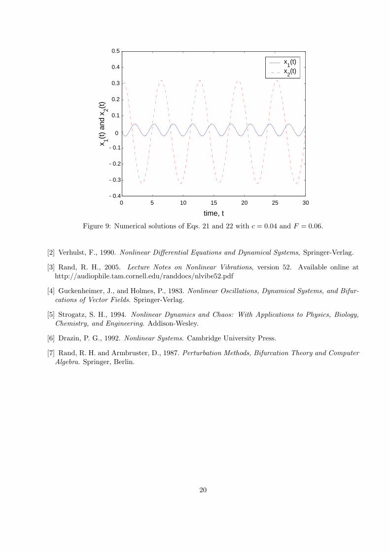
frequency of the forced mode.On numerically solving the above equations for c = 0.04 and F = 0.06, we obtain the steady

state responses shown in Fig. 9. It is seen that the response of x2, i.e., the unforced mode, is at itsnatural frequency, which is one half of the forcing frequency; moreover, this response has a greateramplitude than that of the forced mode itself; and finally, the forced mode responds at the forcingfrequency.

Since the unforced mode is damped, it dissipates energy; that energy comes from the forced mode,showing that the two modes are interacting. This system also provides an example of a motion wheredifferent parts of a system vibrate with different frequencies.

References

[1] Hinch, E. J., 1991. Perturbation Methods, Cambridge University Press.

19

0 5 10 15 20 25 30- 0.4

- 0.3

- 0.2

- 0.1

0

0.1

0.2

0.3

0.4

0.5

time, t

x 1(t)

and

x 2(t)

x1(t)

x2(t)

Figure 9: Numerical solutions of Eqs. 21 and 22 with c = 0.04 and F = 0.06.

[2] Verhulst, F., 1990. Nonlinear Differential Equations and Dynamical Systems, Springer-Verlag.

[3] Rand, R. H., 2005. Lecture Notes on Nonlinear Vibrations, version 52. Available online athttp://audiophile.tam.cornell.edu/randdocs/nlvibe52.pdf

[4] Guckenheimer, J., and Holmes, P., 1983. Nonlinear Oscillations, Dynamical Systems, and Bifur-

cations of Vector Fields. Springer-Verlag.

[5] Strogatz, S. H., 1994. Nonlinear Dynamics and Chaos: With Applications to Physics, Biology,

Chemistry, and Engineering. Addison-Wesley.

[6] Drazin, P. G., 1992. Nonlinear Systems. Cambridge University Press.

[7] Rand, R. H. and Armbruster, D., 1987. Perturbation Methods, Bifurcation Theory and Computer

Algebra. Springer, Berlin.

20