1

Comparison of modeled and measured air-tracer concentrations in the Puget Sound airshed during the summer of 2002. Halstead Harrison Atmospheric Sciences University of Washington Seattle, WA 98195-1640 <harrison@atmos.washington.edu> draft of Jan 28, 2003 Introduction: In 1996 the US Environmental Protection Agency established a program [EMPACT] for environmental monitoring with community public access. One project of this effort [AIRPACT] is underway in the greater Puget Sound metropolitan area of Washington State. As part of this project real-time and predicted simulations of the concentrations of ozone, carbon monoxide, nitric oxide, nitrogen dioxide, and aerosol particles are posted on the web1 in the modeled domain shown in figure 1, on the following page. For many other details of the AIPACT model and program, please refer to Vaughan et al, 2002, which may also be found on the Web2.. In this present note I compare AIRPACT simulations with surface observations for 68 days of June through September during the summer of 2002. I briefly discuss the observations and data quality. Following sections are organized by tracer [O3, CO, NO, NO2, PM2.5] with separate discussions of comparisons, and scores. I conclude with a general discussion, summary, and recommend-ations. Sites and Observations: Tracer concentrations for these comparisons were measured at 33 surface sites operated and maintained by the Puget Sound Clean Air Agency and the Washington State Department of Ecology, as summarized in Table 1, on page 3.

1 http://airpact.ce.wsu.edu/index1.html Click on “recent simulations” 2 http://airpact.ce.wsu.edu/index1.html Click on “background”.

2

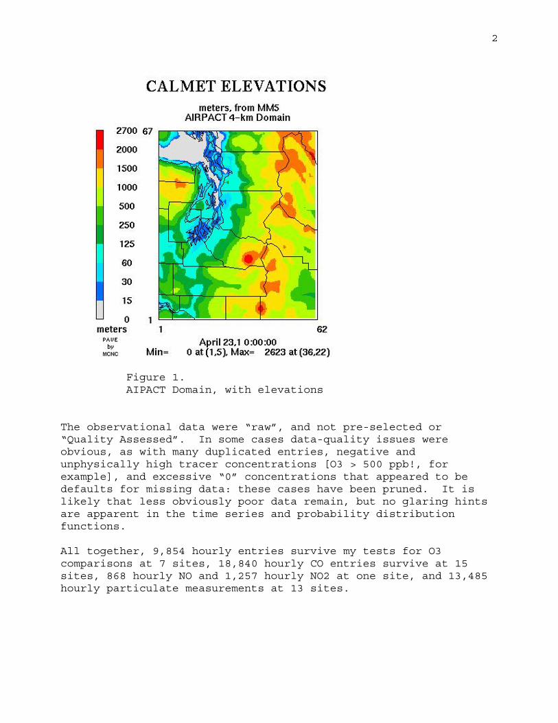
Figure 1. AIPACT Domain, with elevations The observational data were “raw”, and not pre-selected or “Quality Assessed”. In some cases data-quality issues were obvious, as with many duplicated entries, negative and unphysically high tracer concentrations [O3 > 500 ppb!, for example], and excessive “0” concentrations that appeared to be defaults for missing data: these cases have been pruned. It is likely that less obviously poor data remain, but no glaring hints are apparent in the time series and probability distribution functions. All together, 9,854 hourly entries survive my tests for O3 comparisons at 7 sites, 18,840 hourly CO entries survive at 15 sites, 868 hourly NO and 1,257 hourly NO2 at one site, and 13,485 hourly particulate measurements at 13 sites.

3

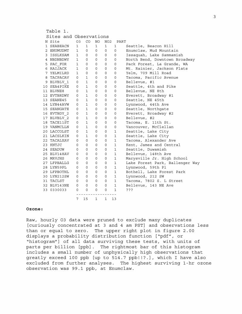
Table 1. Sites and Observations

N Site O3 CO NO NO2 PART 1 SEABEACN 1 1 1 1 1 Seattle, Beacon Hill 2 ENUMUDMT 1 0 0 0 0 Enumclaw, Mud Mountain 3 ISSLKSAM 1 0 0 0 0 Issaquah, Lake Sammamish 4 NBDNBDWY 1 0 0 0 0 North Bend, Downtown Broadway 5 PAC_FOR 1 0 0 0 0 Pack Forest, La Grande, WA 6 RAIJACK 1 0 0 0 0 Mt. Rainier, Jackson Flats 7 YELMILRD 1 0 0 0 0 Yelm, 709 Mill Road 8 TACPACAV 0 1 0 0 0 Tacoma, Pacific Avenue 9 BLVBLV_1 0 1 0 0 0 Bellevue, #1 10 SEA4PIKE 0 1 0 0 0 Seattle, 4th and Pike 11 BLVNE8 0 1 0 0 0 Bellevue, NE 8th 12 EVTBRDWY 0 1 0 0 0 Everett, Broadway #1 13 SEANE45 0 1 0 0 0 Seattle, NE 45th 14 LYN44AVW 0 1 0 0 0 Lynnwood, 44th Ave 15 SEANGATE 0 1 0 0 0 Seattle, Northgate 16 EVTBDY_2 0 1 0 0 0 Everett, Broadway #2 17 BLVBLV_2 0 1 0 0 0 Bellevue, #2 18 TACE11ST 0 1 0 0 0 Tacoma, E. 11th St. 19 VANMCLLN 0 1 0 0 0 Vancouver, McClellan 20 LACCOLST 0 1 0 0 1 Seattle, Lake City 21 LACSLKIN 0 1 0 0 1 Seattle, Lake City 22 TACALXAV 0 0 0 0 1 Tacoma, Alexander Ave 23 KNTJC 0 0 0 0 1 Kent, James and Central 24 SEADUW 0 0 0 0 1 Seattle, Duwamish 25 BLV148AV 0 0 0 0 1 Bellevue, 148th Ave 26 MRVJHS 0 0 0 0 1 Marysville Jr. High School 27 LFPBALLG 0 0 0 0 1 Lake Forest Park, Ballenger Way 28 LYN59PL 0 0 0 0 1 Lynnwood, 59th Pl 29 LFPBOTHL 0 0 0 0 1 Bothell, Lake Forest Park 30 LYN212SW 0 0 0 0 1 Lynnwood, 212 SW 31 TACLST 0 0 0 0 1 Tacoma, 7802 S. L Street 32 BLV143NE 0 0 0 0 1 Bellevue, 143 NE Ave 33 0330033 0 0 0 0 1 ??? ----------------- 7 15 1 1 13

Ozone: Raw, hourly O3 data were pruned to exclude many duplicates [curiously concentrated at 3 and 4 am PST] and observations less than or equal to zero. The upper right plot in figure 2.00 displays a probability distribution function [“pdf”, or “histogram”] of all data surviving these tests, with units of parts per billion [ppb]. The rightmost bar of this histogram includes a small number of unphysically high observations that greatly exceed 100 ppb [up to 514.7 ppb!!?.], which I have also excluded from further analyses. The highest surviving 1-hr ozone observation was 99.1 ppb, at Enumclaw.

4

Figure 2.00: All O3 data The lower-right plot in figure 2.00, shows a scattergram of observed and modeled hourly O3 concentrations [ppb], and the left panel displays the averaged diurnal waves with vertical bars bracketing one standard deviations of the hourly observations, about their means. The abscissa is Pacific Standard Time, PST. Similar plots of comparisons at each site, separately, are appended at the end of this note as figures 2.01-2.07. Table II summarizes some numerical comparisons between the observations and model, for “AllSites”, and for each site separately. Table II:

O3 ppb

<Obs> SD(O) <Mod> SD(M) Bias% RE% R2 Npts Site 26.08 12.90 23.11 11.83 -11.4 56.0 -0.28 9854 AllSites 27.37 11.86 23.03 8.62 -15.9 55.8 -0.66 1431 ENUMUDMT 18.98 10.23 14.20 7.81 -25.1 70.4 -0.71 1368 ISSLKSAM 24.77 12.42 25.79 7.75 4.1 57.4 -0.31 1388 NBDNBDWY 26.75 10.77 23.86 7.80 -10.8 55.3 -0.89 1400 PAC_FOR 38.53 11.11 38.39 9.26 -0.4 40.8 -1.01 1453 RAIJACK 20.50 8.92 14.40 8.45 -29.7 74.4 -1.92 1433 SEABEACN 25.11 10.35 21.54 8.38 -14.2 52.6 -0.63 1381 YELMILRD

5

In Table II the left two columns give the averages, <Obs>, and standard deviations, SD(O), of the observations. The next two columns list the averages and standard deviations of the model, <Mod> and SD(M). The 5th column in these tables lists the net bias between the model and observations, expressed as a percentage: Bias% = 100 [<Mod> - <Obs>] / <Obs> [1] The 6th column, RE%, lists a root-mean-square relative error between model and observation, expressed as a percentage and defined as:

RE% = 100 {(1/Npts) Σ [O(i,j)-M(i,j)]2 )}1/2 / <Obs> [2] In equation [2] the sum is over all observations at paired hours [i = 1 to 24], and sites, j. O(i,j) and M(i,j) are the hourly observations and modeled predictions. The total of these, Npts, is listed in column 8. The 7th column in Table II contains “coefficients of determination”, R2, defined as: R2 = 1 - Σ[O(i,j) - M(i,j)]2 / Σ[O(i,j) - <O>]2 [3] In [3] <O> are the averages over all the observations at each hour [i] and site [j], that is, the central points of the barred curves on the left panels of figures 2.00 - 2.07. Note from the definition of equation [3] that if all observations, O(i,j) were perfectly predicted by the model, M(i,j), then the numerator on the right would be zero, and R2 would be 1.0. Similarly, if for every observation the model predicted M(i,j) equal to the average <O>[or “climatology”] of the observations, then R2 would be zero. Therefore 0 < R2 ≤ 1 is a measure of the "improvement of a model above climatology". All modelers occasionally generate examples with R2 < 0, as is the case for all the comparisons of Table II, but we do not commonly report them3.

3 Some confusion is possible between coefficients of determination, R2, and the squares of Pearson’s correlation coefficient, r2. The latter is always positive, but the former may approach minus infinity.

6

A common feature of figures 2.00-2.07 is that the modeled curves [blue] lead the observed data [red, with vertical dispersion bars] by about two hours, a bias that should be expected to affect the R2 scores that have been quoted above. I have examined the data and my analyses to check whether some error may be infecting the timing of these comparisons, so far without effect4. I have further examined paired “strip-chart” plots of data and model for all tracers, separately at each of the sites and over the whole data period, noting several isolated high peaks of observation and model in both O3 and other tracers that appear to be synchronous. I am therefore tentatively inclined to believe the apparent timing bias to be “real”, and a defect of assumptions or parameters in AIRPACT. It may be useful to ask what improvement in R2 scores might be achieved if biases from both timing and the average amplitudes were arbitrarily “corrected” to zero. While this operation clearly improves the apparent matches among the averaged daily waves of figures 2, it does not significantly improve the RE% or R2 scores, either of the combined [“AllSites”] or the single-site data sets. Specifically, the R2s remain less than zero [“worse than climatology”] at all sites. The National Ambient Air Quality Standards [NAAQS] are concerned with exceedances of “criteria” pollutants, which for O3 are defined as 0.12 ppm [120 ppb] for 1-hour averages, and 0.080 ppm [80 ppb] for 8-hours. Excluding some physically implausible data5, these standards were not exceeded at any site during the present measurements. Carbon Monoxide [CO]: Figure 3.00 similarly shows a combined histogram of CO observations at 15 sites, a scattergram of comparisons between observations and model, and the averaged daily waves. Raw CO data were filtered to remove duplicate, negative, zero, and a few wildly unphysical positive outliers, in this case retaining data pairs in the range 0 < CO ≤ 3 ppm. Considerable variation is observed among the sites, as you should note by inspection of figures 3.01-3.15, appended at the end of this report. 4 The time-axes of all figures in this report are PST (UMT minus 8 hours). Confusion between Daylight and Standard times could account for only half of the apparent time differences in figures 2.0 - 2.7. 5 Scattered O3 “measurements” of several hundred ppb were reported at single sites, contemporaneously with a few ppb, only, at other sites in the network.

7

Figure 3.00: Histogram, Scattergram, and averaged daily waves for CO at all sites.

Table III summarizes some quantitative comparisons between observations and model, in the same format and definitions presented above after Table II. Table III

CO ppm <Obs> SD(O) <Mod> SD(M) Bias% RE% R2 Npts Site 0.72 0.40 0.47 0.29 -35.4 73.1 -0.72 18884 AllSites 0.28 0.18 0.71 0.36 150.3 219.2 -10.55 1482 SEABEACN 0.42 0.15 0.27 0.07 -33.9 51.2 -1.02 844 LACCOLST 0.56 0.38 0.37 0.14 -33.5 76.0 -0.26 1381 TACPACAV 1.01 0.32 0.67 0.28 -33.6 53.2 -1.84 1499 BLVBLV_1 0.79 0.31 0.29 0.17 -62.9 80.4 -3.10 1472 SEA4PIKE 0.72 0.29 0.36 0.17 -50.4 68.9 -1.91 1493 EVTBRDWY 1.02 0.42 0.57 0.30 -44.3 66.8 -1.63 1492 SEANE45 0.73 0.37 0.30 0.15 -59.0 84.2 -1.79 1473 LYN44AVW 0.52 0.27 0.49 0.28 -5.8 72.3 -0.91 1486 SEANGATE 0.98 0.32 0.68 0.28 -30.7 52.5 -1.58 1002 BLVBLV_2 1.01 0.32 0.67 0.28 -33.6 53.2 -1.84 1499 BLVNE8 0.41 0.18 0.27 0.07 -35.2 56.4 -0.74 343 LACSLKIN 0.52 0.41 0.38 0.14 -27.7 83.9 -0.12 930 TACE11ST 0.72 0.29 0.36 0.17 -50.3 68.6 -1.93 1492 EVTBDY_2 0.79 0.30 0.37 0.17 -53.3 69.0 -2.41 996 VANMCLLN

As with O3, the RE% and R2 scores for CO are quite terrible. Of note, perhaps, is the outlier at SEABEACN [Seattle, Beacon Hill],

8

which shows conspicuously worse scores than do the other sites. The Beacon Hill site is the only one reporting a positive concentration bias [Model > Observations]. This site is at the top of a hill, above the intersection of the I-5 and I-90 interstate freeways. At all other sites the detectors are intentionally located close to traffic intersections, at or close to the same horizon, and at these sites the concentration biases are all negative, with Observations > Model. The model, of course, operates at much larger spatial scales, both horizontally and vertically, than are typical of the separation distances between strong CO sources [from traffic] and nearby detectors. For the present purpose of model validation, it is a pity that no CO measurements are co-located with O3 observations at the more remote sites, especially at Enumclaw, the Pack Forest, and Yelm. Most particularly, I recommend that CO measurements be started at the Mud Mountain site, near Enumclaw. This site reports high summertime O3, is sufficiently separated from Seattle’s urban core to be “fair” to both the AIRPACT and MM5 models, and it is reasonably isolated from local traffic. Nitric Oxides: NO and NO2 On the following page are similar plots for NO and NO2. Tables IVa and IVb show numerical summaries in the standard format. Table IVa

NO ppb <Obs> SD(O) <Mod> SD(M) Bias% RE% R2 Npts Site 19.91 25.99 47.91 38.22 140.6 281.0 -3.13 868 SEABEACN Table IVb NO2 ppb <Obs> SD(O) <Mod> SD(M) Bias% RE% R2 Npts Site 18.96 10.96 23.01 11.37 21.4 77.9 -0.82 1257 SEABEACN

NO and NO2 measurements are available only at the site on Seattle’s Beacon Hill. Note that, in common with CO at this site, both NO and NO2 are also over-estimated by the model. Presumably, all three of these gases are dispersed similarly in the near field, but as the conversion of NO to NO2 is delayed somewhat those gases would be expected to behave differently at greater ranges.

9

Figure 4.01: Nitric Oxide at Seattle, Beacon Hill

Figure 4.02: Nitrogen Dioxide at Seattle, Beacon Hill

10

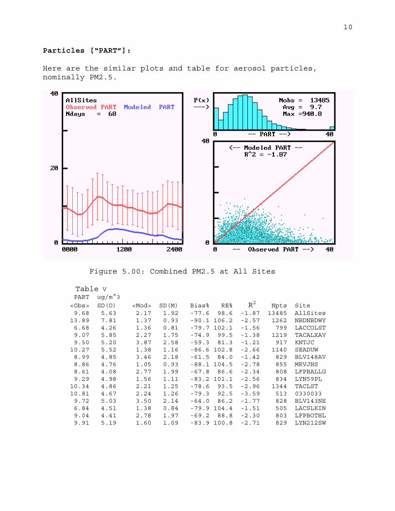
Particles [“PART”]: Here are the similar plots and table for aerosol particles, nominally PM2.5.

Figure 5.00: Combined PM2.5 at All Sites

Table V PART ug/m^3

<Obs> SD(O) <Mod> SD(M) Bias% RE% R2 Npts Site 9.68 5.63 2.17 1.92 -77.6 98.6 -1.87 13485 AllSites 13.89 7.81 1.37 0.93 -90.1 106.2 -2.57 1262 NBDNBDWY 6.68 4.26 1.36 0.81 -79.7 102.1 -1.56 799 LACCOLST 9.07 5.85 2.27 1.75 -74.9 99.5 -1.38 1219 TACALXAV 9.50 5.20 3.87 2.58 -59.3 81.3 -1.21 917 KNTJC 10.27 5.52 1.38 1.16 -86.6 102.8 -2.66 1140 SEADUW 8.99 4.85 3.46 2.18 -61.5 84.0 -1.42 829 BLV148AV 8.86 4.76 1.05 0.93 -88.1 104.5 -2.78 855 MRVJHS 8.61 4.08 2.77 1.99 -67.8 86.6 -2.34 808 LFPBALLG 9.29 4.98 1.56 1.11 -83.2 101.1 -2.56 834 LYN59PL 10.34 4.86 2.21 1.25 -78.6 93.5 -2.96 1344 TACLST 10.81 4.67 2.24 1.26 -79.3 92.5 -3.59 513 0330033 9.72 5.03 3.50 2.14 -64.0 86.2 -1.77 828 BLV143NE 6.84 4.51 1.38 0.84 -79.9 104.4 -1.51 505 LACSLKIN 9.04 4.41 2.78 1.97 -69.2 88.8 -2.30 803 LFPBOTHL 9.91 5.19 1.60 1.09 -83.9 100.8 -2.71 829 LYN212SW

11

Particulate data were also filtered to exclude duplicates, negative entries, and observations out of the range 0 < PART ≤ 40 μg/m3. In the histogram of figure 5 it can be seen that a significant fraction of observations were small [but > 0], and another but lesser fraction exceeded the upper cutoff. General Discussion: The AIRPACT model is doing less well than climatology, for all tracers at all sites. Why? And what should be done about it? Note that for all the tracers except O3, the data reported here were collected at sites close to strong very local sources. The AIPACT model simulates tracer concentrations that are averaged over horizontal scales of a few kilometers, while the measurements sample strong concentration gradients over scales of a few tens of meters. Large positive biases [Observations > Model] are therefore to be expected, as indeed they are observed [excepting at Beacon Hill, where the predictions exceed the observations, perhaps owing to the vertical separation between sources and detectors. The chemistry and transport of O3 formation and loss are complex, with stand-off times of several hours between precursor emissions and maximum O3 concentrations at downwind receptors. The horizontal scales of O3 gradients are comparable to those of the model’s resolution at the suburban [Enumclaw, Lake Sammamish, Yelm] and rural [Pack Forest, Mt. Rainier] sites. It is therefore doubly disappointing that the AIPACT model is not well modeling O3 at these sites, either. Three possibilities are obvious: we have the sources wrong, or the chemistry, or the transport. [Or all at once.] It was my hope at the beginning of this study that effects of transport and chemistry might be separated, at least in part, by comparing CO with O3. The former is a semi-conservative and passive tracer that correlates highly with automotive emissions of both the nitrogen oxides and the hydrocarbon precursors of photosynthetic ozone. Simulating O3 is perhaps the central task of the AIRPACT model. If the CO scores at rural sites were “good”, while O3 scores were “poor”, then we should look to improving the chemistry. If the CO were “poor” also at the rural sites, then a first step would be to reexamine the transport, by winds, from the urban cores to the rural loci of maximum O3.

12

Unfortunately, the present data include no suburban or rural sites with contemporary measurements of both CO and O3. [NOx would be nice, too.] Thus no convincing argument can be sustained by these comparisons as to whether defects of chemistry or transport are more limiting to the skills attainable by the AIRPACT model. That said, suspicions do remain that defects of transport may be severe. Interested readers may wish to look at a related report: “Some comparisons between MM5 forecasts and RAWIN Observations. Is MM5 good enough for air-quality models?” which may be found on the web at <http://www.atmos.washington.edu/~harrison/reports> Summary: I have compared AIRPACT simulations with surface observations for 68 days of June through September during the summer of 2002. For all tracers at all sites the AIPACT model is less skillful than predictions based on climatology. Recommendations: 1. These ozone simulations appear to lead the observations by about two hours. An effort should be made to locate and remove this bias. 2. Carbon Monoxide is semi-conserved on the time scales of transport between the Seattle-Tacoma urban corridor and the more rural sites [Enumclaw, Pack Forest, Yelm] where highest O3 concentrations are observed. Because CO emissions are expected to be roughly proportional to emissions of both the nitrogen oxides and of reactive urban hydrocarbons, ratios of O3/CO, measured at the rural sites would provide better tests of photochemical and transport models than are available with the current data. CO monitoring should begin at Mud Mountain, for starters, with NO/NO2/PM2.5 also if possible. 3. Updates are now planned for both wind- and chemistry models. A similar scorekeeping exercise should be undertaken with next summer’s data. 4. On-the-web displays of AIRPACT simulations should more clearly be labeled as “Experimental and not to be used for operational forecasts”.

13

Figures:

Figure 2.01 O3 at Enumclaw, Mud Mountain

Figure 2.02: O3 at Issaquah, Lake Samamish

14

Figure 2.03: O3 at North Bend, Downtown Broadway

Figure 2.04: O3 at Pack Forest

15

Figure 2.05: O3 at Mt. Rainier, Jackson Flats

Figure 2.06: O3 at Seattle, Beacon Hill

16

Figure 2.07: O3 at Yelm, Mill Road

Figure 3.01 CO at Vancouver, McClellan Ave.

17

Figure 3.02: CO at Everett, Broadway [#2]

Figure 3.03: CO at Tacoma, East 11th Street

18

Figure 3.04: CO at Seattle, Lake City

Figure 3.05: CO at Bellevue, North East 8th

19

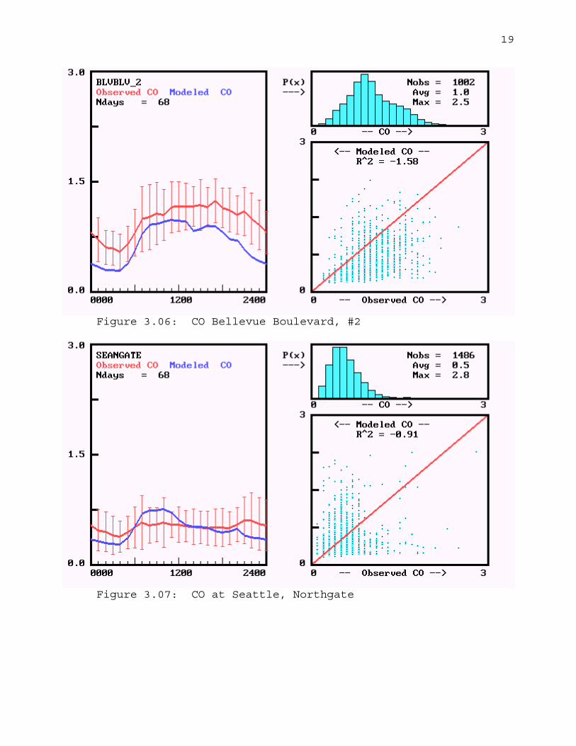
Figure 3.06: CO Bellevue Boulevard, #2

Figure 3.07: CO at Seattle, Northgate

20

Figure 3.08: CO at Lynnwood, 44th Ave

Figure 3.09: CO at Seattle, Northeast 8th

21

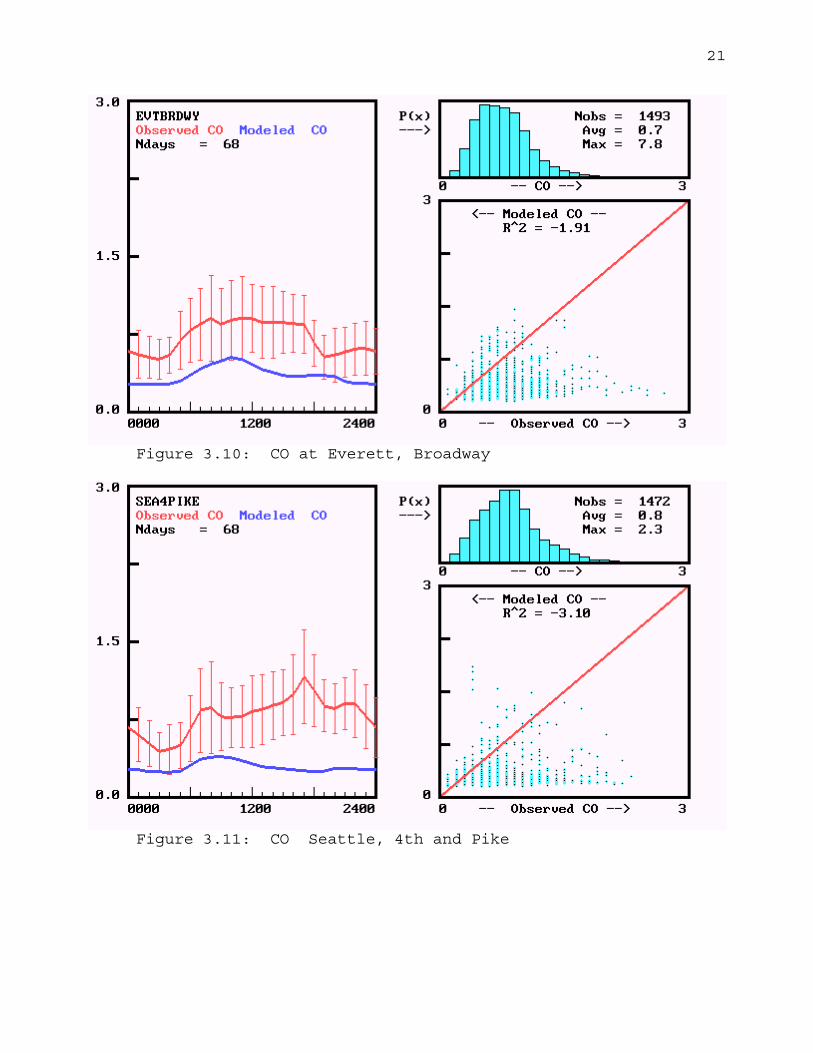
Figure 3.10: CO at Everett, Broadway

Figure 3.11: CO Seattle, 4th and Pike

22

Figure 3.12: CO at Bellevue, Bellevue Boulevard

Figure 3.13: CO at Tacoma, Pacific Avenue

23

Figure 3.14: CO at Seattle, Lake City

Figure 3.15: CO at Seattle, Beacon Hill

24

Figure 5.01: PM 2.5 at Lynnwood, 212 Southwest

Figure 5.02: PM2.5 at Lake Forest Park, Bothell

25

Figure 5.03: PM2.5 at Lake City

Figure 5.04: PM2.5 at Bellevue, 143rd Northeast

26

Figure 5.05: PM2.5 [Site?]

Figure 5.06: PM2.5 at Tacoma, L Street

27

Figure 5.07: PM2.5 at Lynnwood, 59th Place

Figure 5.08: PM2.5 at Lake Forest Park, Ballenger Way

28

Figure 5.09: PM2.5 at Marysville Junior High School

Figure 5.10: PM2.5 at Bellevue, 148th Ave.

29

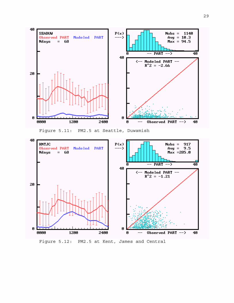
Figure 5.11: PM2.5 at Seattle, Duwamish

Figure 5.12: PM2.5 at Kent, James and Central

30

Figure 5.13: PM2.5 at Tacoma, Alexander Avenue

Figure 5.14: PM2.5 at Seattle, Lake City

31

Figure 5.15: PM2.5 at North Bend, Broadway