1

A branch-and-bound algorithm for the inference of ancestral

amino-acid sequences when the replacement rate varies among

sites

Tal Pupko1,*, Itsik Pe’er2, Masami Hasegawa1, Dan Graur3, and Nir Friedman4

1The Institute of Statistical Mathematics, 4-6-7 Minami-Azabu, Minato-ku, Tokyo 106-8569,

Japan, 2School of Computer Science, Tel Aviv University, Ramat Aviv 69978, Israel,

3Department of Zoology, George S. Wise Faculty of Life Sciences, Tel Aviv University, Ramat

Aviv 69978, Israel, 4School of Computer Science and Engineering, Hebrew University, Jerusalem

91904, Israel

*To whom correspondence should be addressed:

e-mail: tal@ism.ac.jp

Tel: 81-3-5421-8780

Fax: 81-3-5421-8796

Running head: Branch & bound algorithm for ancestral sequences.

Key words: ancestral sequence reconstruction, rate variation among sites, branch and

bound, gamma, molecular evolution

2

Abstract

Motivation: We developed an algorithm to reconstruct ancestral sequences, taking into

account the rate variation among sites of the protein sequences. Our algorithm maximizes

the joint probability of the ancestral sequences, assuming that the rate is gamma

distributed among sites. Our algorithm provably finds the global maximum. The use of

joint reconstruction is motivated by studies that use the sequences at all the internal nodes

in a phylogenetic tree, such as, for instance, the inference of patterns of amino-acid

replacements, or tracing the biochemical changes that occurred during the evolution of a

protein along a predefined lineage.

Results: We give an algorithm that guarantees finding the global maximum. Our method

is applicable for large number of sequences, because of the efficient search method. We

analyze ancestral sequences of five homologous genes, exploring the effect of the amount

of among-site-rate-variation and the degree of sequence divergence on the inferred

ancestral states.

Availability and supplementary information: http://evolu3.ism.ac.jp/~tal/

Contact: tal@ism.ac.jp

3

1. Introduction

By using extant sequences and the phylogenetic relationship among them, it is possible to

infer the most plausible ancestral sequences from which they have been derived.

Maximum likelihood (ML) is a general estimation paradigm, which has been widely

utilized in evolutionary studies (Felsenstein 1981, review in Whelan et al. 2001).

Maximum likelihood algorithms for ancestral sequence reconstruction were developed by

Yang et al. (1995), Koshi and Goldstein (1996), and Pupko et al. (2000), and have been

shown to be more accurate than maximum parsimony reconstructions (Zhang and Nei

1997). Yang (1999) distinguished between two variants of ancestral ML reconstruction:

“joint” and “marginal.” In “joint” reconstruction, one finds the set of all the HTU

(hypothetical taxonomic unit; internal node) sequences. In the “marginal” case, one infers

the most likely sequence in a specific HTU. The results of these two estimation methods

are not necessarily the same (Pupko et al. 2000). The use of “joint” reconstruction is

motivated by studies that use the sequences at all the internal nodes in a phylogenetic

tree, such as, for instance, for inferring patterns of amino-acid replacement or the number

of homoplasies in a tree.

The rate of evolution is not constant among amino-acid sites (Uzzell and Corbin 1971;

Yang 1993). Yang and Wang (1995) stated that “the most worrying assumption made in

the model of Felsenstein (1981) is that substitution rates are constant across sites, which

is unrealistic at least for sequences with biological functions”. The gamma distribution

was used by Nei and Gojobori (1986) and Jin and Nei (1990) to model among-site-rate

variation for nucleotides (see also, Ota and Nei 1994; Rzhetsky and Nei 1994; Yang

4

1994). Using gamma distribution to model among site rate variation was found to be an

important factor in the fitting of models to data (Yang 1996).

Yang (1999) devised an algorithm for “marginal” reconstruction that takes into account

the rate variation among sites. To date, however, there are no “joint” reconstruction

algorithms that take rate variation into account. In this study, we present a branch-and-

bound algorithm to reconstruct ancestral amino-acid sequences for gamma-distributed

rates of amino-acid replacement.

Using this new algorithm, we analyze five groups of homologous genes that had been

previously used in ML-ancestral-sequence-reconstruction studies. We compare the results

obtained from gamma-based ancestral-sequence reconstruction to those obtained without

the assumption of rate variation among sites.

2. Data and Methods

Suppose that the distance between two sequences is d. i.e., on average, we expect d

replacements per site. What is the distribution of this rate among sites? Models that do

not take this variation into account assume that the variance among sites is zero, i.e., that

all sites have the same replacement probability. Models that take this variation into

account assume that at each position, the average number of replacements is d × r, where

the parameter r is sampled from some predefined probability distribution. Since the mean

rate over all sites is d, the mean of r is equal to 1. Yang (1993) suggested the gamma

distribution with parameters α and β as the distribution of r:

5

(1) ∞<<Γ

= −− rrerg r 0)(

),;( 1αβα

αββα

The mean of the gamma distribution is α/β, and since this mean must equal 1, α = β

(Yang 1993). The α parameter is estimated from the data (see below). In this study the

discrete gamma model with k categories is used to approximate the continuous gamma

distribution is used (Yang 1994).

We assume that different sites evolve independently. Thus, we reconstruct ancestral

sequences one site at a time. Hereafter, we address the reconstruction of a single site (for

all HTUs). Let AV (ancestral vector) be the vector of character assignments to all the

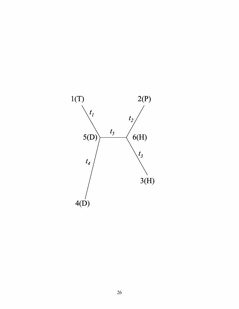
HTUs. For example, we consider the tree in Fig. 1, and use notation of that figure. For

this tree, the AV is {D, H}. The probability of this AV given a rate parameter r is:

(2) { }( ) ( ) ( )

( ) ( ) ( )355

41D

,H,H,P,H,H,D

,D,D,T,DH,D

trPtrPtrP

trPtrPPrP

⋅×⋅×⋅

×⋅×⋅×=

where PD is the frequency of aspartic acid (D) in the data, and ( )121 ,, trAAAAP ⋅ is the

probability that amino acid AA1 will be replaced by amino acid AA2 along a branch of

length t1. Since r at each position is unknown, to calculate the probability of {D, H}, we

average P({D, H}) over different r categories:

(3) { }( ) ( ) ( )i

k

ii rrPrPP =×= ∑

=1

H,DH,D

Thus, we have a method to evaluate the likelihood of each AV, and the most likely AV

can be identified. Yang et al. (1995) first introduced this approach for the reconstruction

6

of ancestral sequences in the simple case of a homogenous rate among sites, and here we

extend it to the more general heterogeneous case.

In this study, models based on amino acid sequences were used. The replacement

probabilities among amino acids were calculated with the JTT matrix (Jones et al. 1992)

for nuclear genes and the REV model (Adachi and Hasegawa 1996) for mitochondrial

genes. However, the approach presented here is also valid for nucleotide sequences and

for any substitution model.

For a phylogenetic tree with m HTUs there are 20m different AVs to be evaluated in order

to find the most likely AV. This number can be reduced to cm, where c is the number of

amino acids that are actually found at a position. For example, if only leucine and

isoleucine are observed at a specific position, one can assume that no other amino acids

except these two would be present in the most likely AV. Hence, in this example there

are only two possible characters for each HTU, and the total number of possible AVs is

2m. Nevertheless, if c is larger then 1, cm increases exponentially with m. The

consequence of this exponent is that for trees with many OTUs and, hence, many HTUs,

it is impractical to evaluate all the possible reconstructions. Pupko et al. (2000) devised a

dynamic programming algorithm for the homogenous case. This algorithm reduces the

number of computations to a linear function of m, and it was integrated into the PAML

software (Yang, 1999). This algorithm guarantees the identification of the most likely set

of ancestral sequences. However, this algorithm is inapplicable when r is gamma

distributed because of the different expressions that have to be maximized (see below).

Hence, a branch-and-bound algorithm for ancestral sequence reconstruction assuming

ASRV (among-site-rate variation) is developed in this study. This is an exact algorithm

that guarantees finding the global maximum likelihood. Although this algorithm is not

7

polynomial in the number of OTU’s, our method is applicable for large numbers of OTUs

because of the efficient search algorithm.

3. Algorithm

Recall, that we assume independence of the stochastic process among sites and, hence,

restrict the subsequent description to a single site. We also describe our algorithm in

terms of amino acids, though the algorithm is general and can be applied to nucleotide or

codon-based models as well.

The input to our problem consists of the phylogenetic tree (with branch lengths), a prior

distribution over possible rates, and a vector o of observations of characters at the leaves

(which correspond to the observed amino-acids at this site in current-day taxa). Our aim

is to find a joint assignment of characters to the internal nodes, whose likelihood is

maximal given the observations.

We start by describing why dynamic programming is inapplicable to this problem. Such

solutions are based on a ``divide and conquer'' property of standard phylogenetic trees;

once we assign a character to an internal node, we break the problem into two

independent sub-problems. When we introduce rate variation, this ``divide and conquer''

property fails - in order to separate the tree into two parts, we need to assign a value to an

internal node and also fix the rate. Indeed, a dynamic programming algorithm for

computing the likelihood of observation in ASRV models uses exactly these joint

assignments (to an internal node and to the rate) in order to decompose recursively the

likelihood computation. However, if we want to perform joint reconstruction we cannot

8

use this decomposition. The joint reconstruction requires finding the assignment to the

internal nodes that will be most likely for all the rates. This reconstruction can differ from

the maximal reconstruction given any particular rate.

Our approach is to search the space of potential reconstructions. Given a putative

reconstruction or partial reconstruction (that assigns values only to some of the internal

nodes), we can compute its likelihood using the dynamic programming procedure

discussed above. Thus, we can define a search space that consists of partial

reconstructions. We can navigate in this space from one partial reconstruction to another

by assigning values to an additional internal node. Our aim is to systematically traverse

this space and find the full reconstruction with maximum likelihood.

Of course, since there is an exponential number of reconstructions, we cannot hope to

traverse all of the space. Instead, we use branch-and-bound search. The key idea of such a

procedure is to prune regions of the search space by computing an upper bound on the

quality of all solutions within the region. Thus, if the upper bound of a region is lower

than a solution that was encountered earlier in the search, then the region can be pruned

from the search. This process is repeated until all possible reconstructions were either

evaluated or pruned.

To carry out this idea we need to upper bound the likelihood of all possible extensions of

a partial reconstruction σ. Thus, we compute a function b(σ) such that

(4) ( ) ( ) ( )oPb C σσ σσ ′≥ ∈′max

where C(σ) is the set of all extensions of σ. (An extension to a partial reconstruction is an

assignment of characters to the internal nodes that are not reconstructed in the partial

9

reconstruction.) We use the bound as follows: if we already found a reconstruction σ*

whose likelihood is higher than b(σ), then we do not need to consider any extension of σ

(since they are provably worse than the best reconstruction). The details of the procedure

involve two key components: (a) methods for computing bounds, and (b) strategy for

determining the order in which to traverse the space of reconstructions that are still

“viable'' given the current bounds.

In this work, we examine two types of upper bounds. The first is based on the observation

that the probability of a partial reconstruction is the sum of the probabilities of the

complete reconstructions that are consistent with it. More precisely,

(5) ( ) ( ) ( )( )

( )oPoPoPC

C σσσσσ

σσ =′≤′ ∑∈′

∈′max

The second bound, is based on the following inequality:

(6) ( ) ( ) ( ) ( ) ( ) ( ) ( ) ( )rPorPrPorPoPr

Cr

CC ,max,maxmax σσσ σσσσσσ ′≤′=′ ∑∑ ∈′∈′∈′

Observe, that ( )orP ,max σσ is the maximum likelihood of an ancestral reconstruction

with a constant rate of evolution r. This can be calculated efficiently using dynamic

programming as in Pupko et al. (2000). In practice, we compute both bounds and use the

smaller value of the two as the bound.

The second issue is the strategy for expanding the search. We need to traverse all possible

reconstructions. We do so by a depth-first search (DFS) that starts with the empty partial

10

reconstruction, and recursively extends it. In each extension step our procedure selects an

HTU that was not assigned in the current reconstruction and considers the possible

assignments to this HTU and recursively expands each one in turn. When the procedure

reaches a complete reconstruction it compares it to the best one found so far, and if it has

higher likelihood, then it records the new solution as the best one. Such a procedure

systematically searches all possible solutions and is thus impractical. By using the idea of

“branch and bound” we prune parts of the search space by using upper bound. The

modified DFS procedure is this:

procedure Reconstruct begin

σ* ← {} // empty set. BestScore ← -∞.

DFS( {} ) return σ*

end procedure DFS ( σ ) begin if σ is a full reconstruction then begin if P(σ|o) > BestScore then begin σ* ← σ BestScore = P(σ|o) end end else // sigma is a partial reconstruction begin if B(σ) ≤ BestScore then return // Pruned σ and all its extensions else begin // σ is not pruned, try to extend it let H be an HTU not assigned in σ for each a ∈ ∑ begin σ’ ← σ ∪ { H = a } // Extend σ DFS( σ’ ) end end end end

This abstract description of the procedure leaves open certain issues, to be decided by the

implementer. It allows choice of the order in which we instantiate HTUs during DFS, and

11

the order in which try to extend them. The intuition is that we first want to search those

assignments that are more likely to be correct. This will yield high scores during early

parts of the search and facilitate more aggressive pruning. To guide the search towards

promising candidates, we compute marginal probabilities for each amino acid for each

node. At each point during the search where we need to choose the next node to be

assigned an amino acid, or the amino acid to be assigned, we choose the assignment with

the highest marginal probability. Thus, we first assign value to the node for which we are

most certain about its value in the reconstruction. After assigning the amino acid to this

node, we turn to the node with the second highest marginal probability. This way the first

complete assignment is always the best marginal reconstruction. Thus, the first candidate

reconstructions would have a high probability. This increases the chance that the bounds

in subsequent moves would be lower than the best reconstruction found so far, i.e., high

chances of pruning the search tree. Furthermore, using such strategy, it is more likely that

the search tree is pruned at the nodes near the root, which helps prune out larger regions

in subsequent moves. This strategy focuses the search on promising directions.

Using our method we find the most likely reconstruction in each position. The likelihood

of this reconstruction can be easily expressed as posterior probabilities, following Yang et

al. (1995). Furthermore, to estimate the reliability of the reconstruction at each specific

node, we followed Yang et al. (1995), and used the marginal probabilities. Thus, our

program output for each position both its probability and the marginal probabilities of

each of the character in each node.

Our algorithm assumes as input a pre-chosen phylogenetic tree. However, in many

practical cases, the tree is uncertain. In order to take into account the uncertainty of the

12

phylogenetic tree, we analyze the ancestral sequence reconstruction based on several

candidate trees, and evaluate the differences.

4. Numerical examples

To demonstrate our algorithm, we choose to analyze five genes that were previously

analyzed using ML-ancestral sequence reconstruction. The datasets are: (1) Lysozyme c.

69 representative sequences were chosen. ML based analysis of a limited number of

sequences of the lysozyme c was done e.g., by Yang, et al. (1995). (2) Mitochondrial

cytochrome oxidase subunit I, and (3) Mitochondrial cytochrome oxidase subunit II. In

each of these genes, 34 sequences are analyzed. ML-based ancestral sequences of

cytochrome oxidase subunits I and II were reconstructed by Andrews and Easteal (2000).

(4) Forty-nine opsin sequences. ML ancestral opsin sequences based on a smaller dataset

were previously analyzed to study the evolution of red and green color vision in

vertebrates (Yokohama and Radlwimmer, 2001; Yokohama and Radlwimmer, 1999; Nei

et al. 1997). (5) ML-based ancestral sequences were also inferred from 73 steroid

receptor sequences. Recently, Thornton (2001) analyzed a subset of 45 out of these 73

sequences for “computational efficiency.” The advantage of using several datasets is to

study the effect of different sequences, different tree topologies and different gamma

parameters on our algorithm. Sequences were aligned using ClustalX (Thompson et al.

1997). Positions with gaps were excluded from the analysis. Alignments and trees are

shown at http://evolu3.ism.ac.jp/~tal/.

The ML tree topologies for the lysozyme c and opsin datasets were obtained using the

MOLPHY software (Adachi and Hasegawa 1996). For cytochrome oxidase subunit II,

13

and I tree topologies was taken from Murphy et al. (2001). The tree topology for the

steroid receptor was taken from Thornton (2001). We note that in many cases, the

likelihood of alternative trees for each gene are not significantly different from one

another. While alternative topologies can be of great importance in phylogenetic studies,

these alternative topologies have small influence on the performance of our algorithm.

Hence a single topology was assumed for each dataset. Amino-acid replacements were

assumed to follow the JTT model for the nuclear genes, and the REV model for the

mitochondrial genes. Branch lengths for each tree were optimized twice – with and

without assuming among-site rate variation.

The alpha parameter of the gamma distribution was estimated with the ML method. To

infer the ancestral sequences, the discrete gamma distribution with 4 categories was used

(Yang 1994). The most likely α parameters found for each dataset are shown in Table 1.

Some genes exhibit very high levels of among-site-rate variation (e.g., mitochondrial

cytochrome oxidase subunit I), while other that show more homogenous distribution of

rates (e.g., steroid receptor sequences).

The log-likelihoods of the 5 gene trees used in this study (with and without the ASRV

assumption) are given in Table 2. The substantial differences between the likelihood with

and without assuming ASRV suggest the existence of high rate variation among sites.

To compare between the different models, the Akaike Information Criterion (AIC)

defined as AIC = -2 × log likelihood +2 × number of free parameters was used

(Sakamoto et al. 1986). A model with a lower AIC is considered a more appropriate

model (Sakamoto et al. 1986). In the gamma model, an additional free parameter is

assumed, i.e., the shape parameter α of the gamma distribution. The AIC differences

14

between the two models (Table 2) are considered highly significant (Sakamoto et al.

1986).

We further compared the log-likelihoods of the reconstructions with and without gamma

(Table 2). The AIC differences again favor the ASRV model for all five trees. Thus, the

assumption of rate variation among sites yielded a significantly more likely tree-branch

lengths and more likely ancestral-sequence reconstructions.

The differences between the ancestral amino-acid reconstructions under the two models

for the 5 genes are summarized in Table 3. One hundred and forty eight differences were

found. Most differences were found in the steroid receptor gene. This is apparently due to

the high rate of evolution of this gene relative to the other genes.

For each internal node, and for each position there are 20 possible amino-acid

assignments. Denote by h the number of internal nodes, and by l the length of the

sequence. Thus, the complete “search-tree” has the size of l·20h. In other words, there are

l·20h nodes in the search-tree. The minimum number of nodes that must be visited is

l·h·20. Consequently, we define the efficiency as:

(7) Efficiency = minimum number of nodes / the number of nodes visited

The efficiency of the algorithm for the five genes together with the running time in

seconds is summarized in Table 4.

5. Discussion

15

Ancestral sequence reconstruction is widely used in evolutionary studies (e.g., Zhang et

al. 1998). In this study, joint reconstruction method of ancestral sequences is

implemented (Yang et al. 1995). This method assigns a set of characters to all interior

nodes simultaneously (Yang 1999). In the PAML software (Yang 1999), the gamma

model is implemented only for the marginal reconstruction (Yang et al. 1995, Yang

1999). Using our branch-and-bound algorithm, we were able to find the global most

likely ancestral-sequence reconstruction for trees with a large number of sequences.

Differences in the AIC values between the homogeneous rate model and the gamma

model indicate that the latter is more appropriate. This was true for all the genes. The

largest AIC differences were found for genes with high levels of among-site-rate-

variation (opsin and co1). Interestingly, the difference in AIC was bigger for the steroid

receptors than for lysozyme c which have lower alpha. This indicates that there is no

direct relationship between the increase in the fit of the model to the data and the alpha

parameter. Nevertheless, all AIC differences were above 250. These values suggest a

very significant difference between the two models.

It was expected that the number of differences between the ancestral amino-acid

sequences with and without the assumption of among-site-rate-variation would be

correlated to the alpha parameter. This pattern was not found: most differences were

found in the steroid receptor gene, while the alpha parameter for this gene indicates low

level of among-site-rate-variation. Our results suggest that the degree of evolutionary

divergence is more important than the alpha parameter. The total branch length of the

steroid receptor is more than three times the total branch length of lysozyme c and more

than six times the total branch length of the other genes (Table 1). Thus, when the

16

evolutionary divergence is high, the uncertainty in the ancestral sequences increase. In

such cases the underlying model assumed becomes more important.

The very high efficiency values (Table 4) are the result of two components: the tight

bounds, and the procedure based on the marginal probabilities to determine the order of

nodes in the search tree. The steroid receptor gene was the least efficient (97.7%, Table

4). This is possible due to the high rate of evolution in this gene. The average efficiency

of the algorithm for all five genes was above 99% (Table 4). This result is heartening.

Our goal was to develop an efficient algorithm to find the global most likely set of

ancestral sequences assuming among-site-rate-variation. Not only this was achieved for

all five genes, the efficiency values and the running times indicate that even bigger trees

and longer sequences can be analyzed.

The maximum likelihood framework in this paper makes some very explicit assumptions.

For example in some specific positions, where positive Darwinian selection is suspected,

selection forces might be responsible for deviation from the assumed replacement matrix.

Another limitation of our method (and of all other methods currently available) is the

assumption that different sequence positions evolve independently. This is most probably

an unrealistic assumption. A better approach would be to assume that amino-acid

positions, which are close to one another in the 3D structure of the protein, affect one

another. Modeling such spatial correlations is an exiting topic for future studies.

Acknowledgment

17

T.P. is supported by a grant from the Japanese Society for the Promotion of Science

(JSPS). I.P. is supported by the Clore Foundation.

References

Adachi, J., and Hasegawa, M. (1996). MOLPHY: programs for molecular phylogenetics

based on maximum likelihood, version 2.3. Institute of Statistical Mathematics, Tokyo,

Japan.

Andrews, T.D., and Easteal. S. (2000). Evolutionary rate acceleration of cytochrome c

oxidase subunit I in simian primates. J. Mol. Evol. 50:562-568.

Felsenstein, J. (1981). Evolutionary trees from DNA sequences: a maximum likelihood

approach. J. Mol. Evol. 17:368-376.

Jin, L., and Nei, M. (1990). Limitations of the evolutionary parsimony method of

phylogeny analysis. Mol. Biol. Evol. 7:82-102.

Jones, D.T., Taylor, W.R., and Thornton, J.M. (1992). The rapid generation of mutation

data matrices from protein sequences. Comput. Appl. Biosci. 8:275-282.

Koshi, J.M., and Goldstein, R.A. (1996). Probabilistic reconstruction of ancestral protein

sequences. J. Mol. Evol. 42:313-320.

Murphy, W. J., E. Eizirik, W. E. Johnson, Y. P. Zhang, O. A. Ryder and S. J. O'Brien.

18

(2001). Molecular phylogenetics and the origins of placental mammals. Nature 409:614-

618.

Nei, M., and Gojobori, T. (1986). Simple methods for estimating the number of

synonymous and nonsynonymous nucleotide substitutions. Mol. Biol. Evol. 3:418-426.

Nei, M., Zhang, J., and Yokoyama, S. (1997). Color vision of ancestral organisms of

higher primates. . Mol. Biol. Evol. 14:611-618.

Ota, T., and Nei, M. (1994). Estimation of the number of amino acid substitutions when

the substitution rate varies among sites. J. Mol. Evol. 38:642-643.

Pupko, T., Pe’er, I., Shamir, R., and Graur, D. (2000). A Fast algorithm for joint

reconstruction of ancestral amino-acid sequences. Mol. Biol. Evol. 17:890-896.

Rzhetsky, A., and Nei, M. (1994). Unbiased estimates of the number of nucleotide

substitutions when a substitution rate varies among different sites. J. Mol. Evol. 38:295-

299.

Sakamoto, Y., Ishiguro, M., and Kitagawa, G. (1986). Akaike Information Criterion

Statistics. D. Reidel, Dordrecht.

Thompson, J.D., Gibson, T.J., Plewniak, F., Jeanmougin, F. and Higgins, D.G. (1997)

The ClustalX windows interface: flexible strategies for multiple sequence alignment

aided by quality analysis tools. Nuc. Acid Res. 24:4876-4882.

19

Thorntom, J.W. (2001) Evolution of vertebrate steroid receptors from an ancestral

estrogen receptor by ligand exploitation and serial genome expansions. Proc. Natl. Acad.

Sci. USA 98:5671-5676.

Uzzell, T., and Corbin, K.W. (1971). Fitting discrete probability distributions to

evolutionary events. Science 172:1089-1096.

Whelan, S., Li, P., and Goldman, N. (2001). Molecular phylogenetics: state-of-the-art

methods for looking into the past. TRENDS in Genetics 17:262-272.

Yang, Z. (1993). Maximum-likelihood estimation of phylogeny from DNA sequences

when substitution rates differ over sites. Mol. Biol. Evol. 10:1396-1401.

Yang, Z. (1994). Maximum likelihood phylogenetic estimation from DNA sequences

with variable rates over sites: Approximate methods. J. Mol. Evol. 39:306-314.

Yang, Z., Kumar, S., and Nei, M. (1995). A new method of inference of ancestral

nucleotide and amino acid sequences. Genetics 141:1641-1650.

Yang, Z., and Wang, T. (1995). Mixed model analysis of DNA sequence evolution.

Biometrics 51:552-561.

Yang, Z. (1996). Among-site rate variation and its impact on phylogenetic analysis.

Trends. Ecol. Evol. 11:367-372.

20

Yang, Z. (1999). PAML: A Program Package for Phylogenetic Analysis by Maximum

Likelihood. Version 2.0. University College London, London.

Yokoyama, S., and Radlwimmer, F. B. (1999). The molecular genetics of red and green

color vision in mammals. Genetics. 153:919-932.

Yokoyama, S., and Radlwimmer, F. B. (2001). The molecular genetics and evolution of

red and green color vision in vertebrates. Genetics. 158:1697-1710.

Zhang, J., and Nei, M. (1997). Accuracies of ancestral amino acid sequences inferred by

the parsimony, likelihood, and distance methods. J. Mol. Evol. 44:S139-S146.

Zhang, J., Rosenberg, H.F., and Nei, M. (1998). Positive Darwinian selection after gene

duplication in primate ribonuclease genes. Proc. Natl. Acad. Sci. USA 95:3708-3713

21

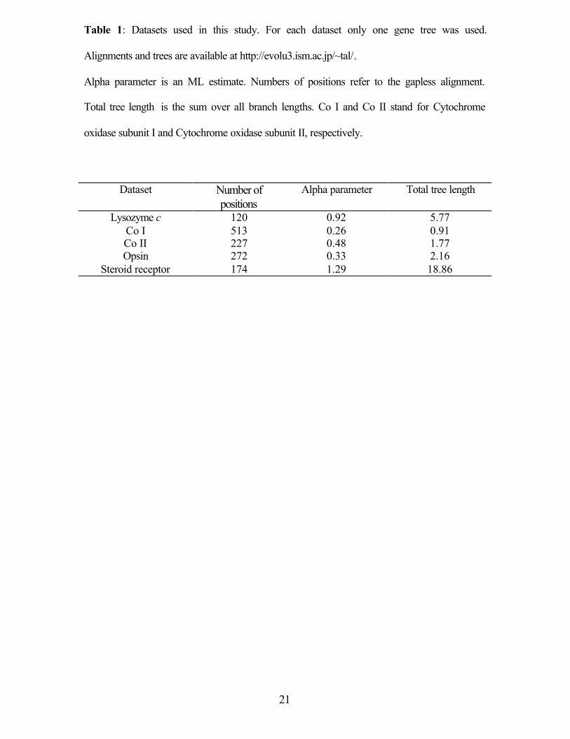
Table 1: Datasets used in this study. For each dataset only one gene tree was used.

Alignments and trees are available at http://evolu3.ism.ac.jp/~tal/.

Alpha parameter is an ML estimate. Numbers of positions refer to the gapless alignment.

Total tree length is the sum over all branch lengths. Co I and Co II stand for Cytochrome

oxidase subunit I and Cytochrome oxidase subunit II, respectively.

Dataset Number of

positions Alpha parameter Total tree length

Lysozyme c 120 0.92 5.77 Co I 513 0.26 0.91 Co II 227 0.48 1.77 Opsin 272 0.33 2.16

Steroid receptor 174 1.29 18.86

22

Table 2: Log-likelihoods of the trees and the ancestral amino-acid reconstruction of the

five datasets. ∆AIC is defined as in Sakamoto et al. (1986). Trees and ancestral-sequence

reconstructions were evaluated either under the assumption of homogenous rate variation

among sites (“Without Γ”), or assuming a gamma distribution of rates among sites

(“With Γ”). Positive ∆AIC values indicate that the ASRV model is better than the

homogenous model. Co I and Co II stand for Cytochrome oxidase subunit I and

Cytochrome oxidase subunit II respectively.

Dataset Log likelihood of tree Log likelihood of reconstruction

Without ΓΓ With ΓΓ ∆AIC Without ΓΓ With ΓΓ ∆AIC

Lysozyme c -3809.02 -3669.51 277.02 -3886.7 -3759.64 252.12

Co I -4268.65 -4014.57 506.16 -4421.5 -4133.72 573.56

Co II -2720.59 -2594.06 251.06 -2833.71 -2665.41 334.6

Opsin -4216.49 -3920.64 589.7 -4257.64 -3967.03 579.22

Steroid receptor

-9417.04 -9169.25 493.58 -9744.79 -9584.19 319.2

Total -25144.3 -24110.0 2125.52 -24955.5 -23879.5 2066.7

23

Table 3: Differences between ancestral amino-acid reconstructions inferred with and

without the assumption of rate variation among sites. The numbers in the second column

refer to the position in the gapless alignment. In some positions more than one difference

was found. The total number of differences is summarized in the third column. In all

other nodes and positions, the two models yielded identical ancestral amino-acid

reconstructions.

Dataset Positions in which difference was found

Total number of differences

Lysozyme c 23, 37, 43, 117 10 Cytochrome oxidase subunit I 3, 488, 489 5 Cytochrome oxidase subunit II 22, 74, 224 9

Opsin 8, 9, 50, 119 9 Steroid receptor 1, 12, 13, 14, 15, 17, 18,

19, 21, 22, 23, 28, 30, 56, 65, 71, 73, 74, 79,

80, 83, 92, 99, 102, 111, 112, 117, 130, 132, 137, 138, 140, 148, 150, 152, 153, 157, 165, 168, 171

133

24

Table 4: Efficiency and running times in seconds for the five genes in this study.

Running times were computed on a 600 MHZ Pentium machine with 256 MB RAM.

Dataset Efficiency (%) Running time (sec)

Lysozyme c 99.62 4668 Cytochrome oxidase subunit I 99.98 4373 Cytochrome oxidase subunit II 99.93 1905

Opsin 99.95 5199 Steroid receptor 95.51 8609

Sum 99.95 24756

25

Figure. 1: Unrooted phylogenetic tree with 4 taxa. All nodes are labeled: OTUs (1-4) and

HTUs (5-6). ti are the branch lengths. Capital letters in parentheses are one letter

abbreviations for amino acids. The AV for this tree is {D,H}. The ancestral vector (AV)

is ordered such that the first amino acid (D) corresponds to the internal node (HTU) with

the smallest label.

26

t1

t3

t2

t5

t4

1(T)

3(H)

4(D)

2(P)

5(D) 6(H)

t1

t3

t2

t5

t4

1(T)

3(H)

4(D)

2(P)

5(D) 6(H)