A BRANCH AND BOUND ALGORITHM FOR … · a branch and bound algorithm for resource leveling problem a thesis submitted to the graduate school of natural and applied sciences of middle

A BRANCH AND BOUND ALGORITHM FOR RESOURCE LEVELING PROBLEM

A THESIS SUBMITTED TO THE GRADUATE SCHOOL OF NATURAL AND APPLIED SCIENCES

OF MIDDLE EAST TECHNICAL UNIVERSITY

BY

MUSTAFA ÇAĞDAŞ MUTLU

IN PARTIAL FULFILLMENT OF THE REQUIREMENTS

FOR THE DEGREE OF MASTER OF SCIENCE

IN CIVIL ENGINEERING

AUGUST 2010

Approval of the thesis:

A BRANCH AND BOUND ALGORITHM FOR RESOURCE LEVELING PROBLEM

submitted by MUSTAFA ÇAĞDAŞ MUTLU in partial fulfillment of the requirements for the degree of Master of Science in Civil Engineering Department, Middle East Technical University by, Prof. Dr. Canan Özgen Dean, Graduate School of Natural and Applied Sciences Prof. Dr. Güney Özcebe Head of Department, Civil Engineering Assoc. Prof. Dr. Rıfat Sönmez Supervisor, Civil Engineering Dept., METU Examining Committee Members: Assist. Prof. Dr. Metin Arıkan Civil Engineering Dept., METU Assoc. Prof. Dr. Rıfat Sönmez Civil Engineering Dept., METU Prof. Dr. M. Talat Birgönül Civil Engineering Dept., METU Assoc. Prof. Dr. Murat Gündüz Civil Engineering Dept., METU Alphan Nurtuğ, M.Sc. Project Manager - PMP, 4S Software

Date: 04.08.2010

iii

I hereby declare that all information in this document has been

obtained and presented in accordance with academic rules and

ethical conduct. I also declare that, as required by these rules and

conduct, I have fully cited and referenced all material and results

that are not original to this work.

Name, Last Name : Mustafa Çağdaş Mutlu

Signature :

iv

ABSTRACT

A BRANCH AND BOUND ALGORITHM FOR

RESOURCE LEVELING PROBLEM

Mutlu, Mustafa Çağdaş

M.S., Department of Civil Engineering

Supervisor: Assoc. Prof. Dr. Rıfat Sönmez

August 2010, 106 Pages

Resource Leveling Problem (RLP) aims to minimize undesired fluctuations in

resource distribution curves which cause several practical problems. Many

studies conclude that commercial project management software packages can

not effectively deal with RLP. In this study a branch and bound algorithm is

presented for solving RLP for single and multi resource, small size networks.

The algorithm adopts a depth-first strategy and stores start times of non-

critical activities in the nodes of the search tree. Optimal resource distributions

for 4 different types of resource leveling metrics can be obtained via the

developed procedure. To prune more of the search tree and thereby reduce

the computation time, several lower bound calculation methods are employed.

Experiment results from 20 problems showed that the suggested algorithm

can successfully locate optimal solutions for networks with up to 20 activities.

The algorithm presented in this study contributes to the literature in two

points. First, the new lower bound improvement method (maximum allowable

daily resources method) introduced in this study reduces computation time

required for achieving the optimal solution for the RLP. Second, optimal

solutions of several small sized problems have been obtained by the algorithm

v

for some traditional and recently suggested leveling metrics. Among these

metrics, Resource Idle Day (RID) has been utilized in an exact method for the

first time. All these solutions may form a basis for performance evaluation of

heuristic and metaheuristic procedures for the RLP. Limitations of the

developed branch and bound procedure are discussed and possible further

improvements are suggested.

Keywords: Resource Leveling Problem, Branch and Bound Method, Discrete

Optimization, Resource Idle Day

vi

ÖZ

KAYNAK DENGELEME PROBLEMĐNĐN ÇÖZÜLMESĐ AMACIYLA

BĐR DAL VE SINIR ALGORĐTMASI GELĐŞTĐRĐLMESĐ

Mutlu, Mustafa Çağdaş

Yüksek Lisans, Đnşaat Mühendisliği Bölümü

Tez Yöneticisi: Doç. Dr. Rıfat Sönmez

Ağustos 2010, 106 Sayfa

Kaynak Dengeleme Problemi (KDP), kaynak çizelgelerindeki istenmeyen

dalgalanmaların asgari düzeye indirilmesini, böylelikle bu dalgalanmaların yol

açabileceği olası sorunların önlenmesini amaçlamaktadır. Proje planlamasında

ve yönetiminde yaygın olarak kullanılan paket programların KDP’ni çözmede

yetersiz kaldıkları çok sayıda araştırmada belirtilmiştir. Bu çalışma kapsamında,

tek ve çok kaynaklı, küçük ölçekli şebekelerde KDP için en optimal çözümü

bulmayı amaçlayan bir dal ve sınır algoritması geliştirilmiştir. Geliştirilen

algoritma derinliğine arama stratejisini esas almakta ve arama ağacının herbir

düğümünde belirli bir aktivite için geçerli bir başlangıç tarihi saklamaktadır. 4

ayrı kaynak dengeleme ölçütü için en optimal çözümü bulabilen yöntem, çok

sayıda alt sınır hesaplama tekniğine yer vererek arama alanını sınırlandırılmaya

çalışmaktadır. 20 iş programı üzerinde yapılan deneyler, geliştirilen

algoritmanın 20 aktiviteli şebekelere kadar olan problemlerde en optimal

çözümleri bulabildiğini göstermiştir.

Sunulan yöntem literatüre iki önemli noktada katkı sağlamaktadır. Öncelikle,

önerilen alt sınır hesaplama tekniği (izin verilebilen en fazla günlük kaynak

tüketimi) en optimal çözümün bulunması için ihtiyaç duyulan hesaplama

vii

zamanının kısaltılmasını sağlamıştır. Ayrıca, bazı küçük ölçekli kaynak

dengeleme problemlerinin çeşitli ölçütler için optimal çözümleri sunularak

gelecekte geliştirilecek sezgisel yöntemlerin performanslarının

değerlendirilmesi amacıyla bir örnek problem seti oluşturulmuştur. Yakın

zamanda önerilmiş olan “atıl kaynak günü” kaynak dengeleme ölçütü için

pekçok problemin en optimal çözümleri literatürde ilk defa bulunmuştur.

Geliştirilen yöntemin kısıtlamaları tartışılmış ve ileride yapılabilecek çalışmalar

ile ilgili önerilerde bulunulmuştur.

Anahtar Kelimeler: Kaynak Dengeleme Problemi, Dal ve Sınır Algoritması,

Kesikli Optimizasyon, Atıl Kaynak Günü

viii

To My Mother

ix

ACKNOWLEDGMENTS

I would like to express my sincere thanks to my supervisor,

Assoc. Prof. Dr. Rıfat Sönmez for the vision, encouragement, comments and

critiques he provided for this work. I am grateful not only for his patient

supports throughout this study, but also for his modesty in sharing his

valuable experiences with me. I know that the insight he provided will guide

me all through my life.

I would like to thank Prof. Dr. M. Talat Birgönül for his understanding and for

his efforts in providing the conditions I needed to complete this study. I am

also indebted to all faculty members and research assistants of the

Construction Engineering and Management Division of Middle East Technical

University. Surely, they all contributed to this work one way or another.

There is no way for me to show how much I appreciate the everlasting

support of my parents, Aysel Bulgu and Nureddin Mutlu. I owe my deepest

gratitude to my aunt Nefise Bulgu who let me benefit from her wisdom and

who has patiently shared all my difficult times in Ankara. Also, my uncle

Aykut Lenger deserves special mention for the guidance he provided with me

for all critical decisions I have ever made. He is surely at the top of my

gratitude list.

I also would like to thank my girlfriend Đrem Onar who has motivated me

more than anybody else could do and who shared all difficulties I

encountered. Without her, one piece of this study, as well as me, would be

lacking. Finally, I would like to express my special thanks to Alper Önen,

Umut Akın and all other friends of mine whose support I felt with me

throughout this study.

x

TABLE OF CONTENTS

ABSTRACT iv

ÖZ vi

ACKNOWLEDGEMENTS ix

TABLE OF CONTENTS x

LIST OF TABLES xii

LIST OF FIGURES xiv

LIST OF ABBREVIATIONS xv

CHAPTER

1. INTRODUCTION 1

2. LITERATURE REVIEW 9

2.1 Heuristic, Metaheuristic and Exact Methods 9

2.2 Heuristic and Metaheuristic Methods for Resource Leveling

Problem 12

2.3 Exact Methods for RLP and Other Scheduling Problems 23

3. BRANCH AND BOUND METHOD 34

3.1 Objective Functions 34

3.1.1 Sum of Squares (SSQR) of Resource Requirements 34

3.1.2 Minimum Absolute Deviation (MinDev) of Resource

Requirements from Uniform Resource Level 35

3.1.3 Resource Idle Days (RID) 37

3.1.4 Resource Idle Days and Maximum Resource Demand

(RID+MRD) 38

3.2 Basics of the Branch and Bound Method 39

3.3 Problem Definition 41

3.4 Characteristics of the Developed Branch and Bound Algorithm 45

3.4.1 Branching from Nodes to New Nodes 45

3.4.2 Determining Lower Bounds for the New Nodes 47

3.4.2.1 Discarding Critical Activities 47

3.4.2.2 Unavoidable Times of Activities 48

3.4.2.3 Allocating Unscheduled (Free) Resources 50

3.4.2.4 Maximum Allowable Daily Resources 55

xi

3.4.3 Choosing an Intermediate Node from Which to Branch

Next and Selecting the Activity to be Scheduled 59

3.4.4 Recognizing Non-promising Nodes and Optimal

Solutions 60

3.5 The Branch and Bound Procedure 61

3.6 Coding the Algorithm 64

4. VALIDATION AND COMPUTATIONAL RESULTS 66

4.1 Validating the Algorithm 66

4.2 Computational Results 68

4.3 Effect of the Maximum Allowable Daily Resources

Improvement on the Performance of the Algorithm 83

5. CONCLUSIONS 86

REFERENCES 90

APPENDICES

A. PROBLEM INPUTS 97

xii

LIST OF TABLES

TABLES

Table 2.1 Heuristic and Metaheuristic Methods for RLP 21-22

Table 2.2 Exact Methods for Scheduling Problems 31-32

Table 4.1 Computational Results (Schedules 1 and 2) 71










Table 4.11 CPU Times Spent by Algorithms with and without Employing

Maximum Allowable Daily Resources Improvement (seconds) 84

Table 4.12 Significance Levels at which Means of the Computation Times

with and without MaxRes Improvement are Different 85

Table A.1 Inputs for Problem No. 1 97












xiii









xiv

LIST OF FIGURES

FIGURES

Figure 3.1 Sample Resource Distribution 35

Figure 3.2 Idle Days on the Sample Resource Distribution of Figure 3.1 38

Figure 3.3 Sample Activitiy on Node Schedule 41

Figure 3.4 Resource Distribution for the Early Start Schedule of Figure 3.3 42

Figure 3.5 Search Tree Established by the Branch and Bound Algorithm 43

Figure 3.6 Optimal Resource Distribution for the Schedule of Figure 3.3 44

Figure 3.7 Resource Distribution of Critical Activities (a) and Unavoidable

Resources 49

Figure 3.8 Resource Distribution After Scheduling Activity 3 (a) and

After Scheduling Additional Resources (b) 53

Figure 3.9 Maximum Allowable Daily Resources (a) and Lower Bound

Calculation According to These Resource Limits (b) 57

Figure 3.10 Search Tree Established by Utilizing Maximum Allowable Daily

Resources Improvement in Addition to the Improvements Given in

Sections 3.4.2.1, 3.4.2.2 and 3.4.2.3 58

xv

LIST OF ABBREVIATIONS

AoA Activity on Arrow

AoN Activity on Node

CPM Critical Path Method

EF Early Finish

ES Early Start

DSS Decision Support System

GA Genetic Algorithm(s)

LF Late Finish

LS Late Start

MaxRes Maximum Allowable Daily Resource Limitation

MinDev Minimum Absolute Deviation

MRD Maximum Resource Demand

NP-Complete Non-deterministic Polynomial-time Complete

NP-Hard Non-deterministic Polynomial-time Hard

PACK Packing Method

PMBOK Project Management Body of Knowledge

PSO Particle Swarm Optimization

RAM Random Access Memory

RCPSP Resource Constrained Project Scheduling Problem

RCPSPDC Resource constrained project scheduling problem with discounted

cash flows

RID Resource Idle Day

RLP Resource Leveling Problem

RRH Release and Rehire

SA Simulated Annealing

sd Standard Deviation

SSQR Sum of Squares

TF Total Float (Slack)

TSP Travelling Salesman Problem

1

CHAPTER 1

INTRODUCTION

Although importance of project planning is recognized in many project based

industries, few companies depend on scheduling skills as much as

construction companies do. Operating under continuously changing

environmental conditions and being involved in complex and unique projects,

which require multidisciplinary collaboration, construction companies have to

develop realistic schedules and update them regularly. It is not only the

nature of the construction business that makes scheduling such a vital task.

Increasing competition within the industry also forces construction companies

to provide products of higher quality, in shorter durations, for lower costs and

under safer working environments. Obviously, it is not possible to achieve

these objectives simultaneously in the absence of an adequate schedule.

As characteristics of the construction business point out, preparation of a

schedule for a construction project requires simultaneous consideration of

several issues. Although scheduling might be perceived as a simple matter of

determining the sequence and timing of activities within a project, a planner

has to cope with a number of constraints and considerations. Precedence

relations, lag times, productivity rates, site availability, working calendars and

climatic conditions are some of the many issues to be considered during the

preparation of a schedule. In addition to these, resource requirements of

activities, availability of resources and shapes of the resource requirement

curves also need to be considered to ensure economical resource utilization.

2

One of the most common reasons why schedules deviate from reality is that,

resources are not carefully considered during planning phase. If resources are

not scheduled together with the activities by considering resource availabilities

and resource graph fluctuations, in other words if resource allocation is not

carried out properly, then there is a high probability that obtained schedule

will fail to successfully model the project in terms of duration and cost.

Obviously, such an unsuccessful schedule would pose a threat for a company

in that it may cause financial losses, problems, dissatisfied clients, bad

reputation etc. In fact, an adequate schedule, which incorporates resources

appropriately, provides competitive advantage to the company from the very

beginning until the end of the project.

One of the most commonly applied scheduling techniques is the critical path

method (CPM). In this method, durations of activities and precedence

relations between them are defined. Schedules are prepared based on these

inputs and illustrated by one of the two popular methods which are activity on

arrow (AoA) or activity on node (AoN) representations. Early start and early

finish times and late start and late finish times of tasks are determined by

forward pass and backward pass calculations respectively. After these

calculations, total floats (slacks) of activities are determined by subtracting

early start times from the late start times. Total floats give an indication of the

amount of allowable delay in starting/completing any activity without

extending overall project duration. If total float of a task is equal to zero, this

means that the activity is a critical one and has to start as soon as its

predecessors are completed. Path or paths consisting of critical activities are

called critical path/paths and the project makespan equals the total duration

required to complete any of these. Theoretically, preparation of a regular CPM

network does not necessarily require resource allocation as long as durations

of activities and precedence relations among them are defined adequately. In

fact, schedules depending on this much consideration are commonly used

within the construction industry, while resource utilization issues are usually

disregarded.

3

If resources required by each activity are assigned on an early start schedule,

in which all tasks are started as soon as possible, it is highly probable that

there will be very high amounts of resource requirements for some periods.

Moreover, if resource utilization graphs are considered, undesired fluctuations

may easily be observed. These are among the major reasons why some

schedules are far from representing actual projects and therefore should be

prevented as much as possible. Scheduling problems try to eliminate such

situations in order to obtain more realistic schedules and to minimize financial

losses due inefficient planning.

One of the scheduling problems commonly addressed by researchers is

Resource Constrained Project Scheduling Problem (RCPSP). In this

problem it is aimed to complete a project as soon as possible using available

amounts of resources. In a feasible solution of RCPSP resource requirements

of activities are lower than or equal to the amount of available resources at

any instant of time. In other words, solution of RCPSP ensures effective use of

available resources so that the project is completed as soon as possible

without exceeding resource limitations.

It has been indicated that early start schedules, inevitably, include undesired

fluctuations in resource utilization graphs over time. Such variations are

known to have several negative impacts from the project management point

of view. Unproductive labor and equipment utilization, increased cost of

temporary facilities, short term employment of the workforce and difficulties in

attracting skilled workforce due to lack of guarantee to provide long term job

opportunities are some of the most significant negative outcomes of these

fluctuations. Frequently rehiring and releasing employees also reduces the

motivation of individuals and makes the establishment of a company culture

difficult. Moreover, companies have to make significant investments on the

training of their staff repeatedly, since the workforce is not stable. Especially,

in construction industry which depends on know-how at individual and

company levels, such fluctuations’ costs to the companies are considerable.

4

Variations in resource demand curves, which might have the negative impacts

listed in the previous paragraph, are addressed by the Resource Leveling

Problem (RLP). The purpose of this problem is to eliminate fluctuations on

the resource demand over time periods throughout the project makespan. A

leveled resource distribution is aimed to be achieved by considering unlimited

amounts of resources. To do this non-critical activities on a CPM schedule are

shifted within their available float times. In a feasible solution of RLP, start

times of activities are adjusted in a manner that resource level variations are

minimized as much as possible. At this point, it might be useful to revisit some

of the major assumptions outlined by Harris (1990) for RLP, which are also

valid for this study.

• Activities are assumed to be time continuous and are not allowed to be

splitted. In other words, once an activity has started it can not be

stopped until completion.

• Resources consumed by activities are assumed to remain constant

from the beginning until the end of the activities, i.e. each activity is

assumed to have a constant rate of utilization of the resources.

• Reductions or extensions in activities’ duration by changing their

resource rates are not allowed.

• The algorithm is not allowed to extend or shorten the project duration.

As the assumptions listed above indicate, extensions in project duration are

not allowed in traditional RLP. However, there are some studies in the

literature which allow project makespan to be extended up to a certain time

limit; e.g. a fraction of initial CPM duration. There are also some studies on

RLP which allow activities to be stopped and restarted, i.e. splitted, although

traditional assumptions do not allow this. It could be said that RLP addressed

in these studies are variations of the traditional RLP. Such considerations, of

course, might be useful for projects from many industries. However, it is

believed that RLP in its traditional format is the most applicable problem for

construction industry.

5

Quantification of the amount of resource fluctuations is an important issue to

be considered while dealing with RLP. Several objective functions have been

devised for this purpose in the literature. Minimization of sum of squares of

resource demands per period, minimization of the absolute differences

between resource demands in consecutive periods and minimization of the

absolute deviations from a uniform or desired resource level are three of the

oldest and most commonly used objective functions. In addition to these,

metrics to minimize the moment of the resource histogram, to minimize the

idle times of the resources and to minimize the rate of releasing and rehiring

resources are also being employed by researchers. Detailed information on

traditional objective functions and on some more innovative metrics is going

to be presented in the following chapters. However, it should be realized at

this point that trying to conform resource utilization graphs to predetermined

shapes usually makes the solution of RLP even more difficult since such

resource distributions most of the times may not be possible due precedence

constraints. Moreover some metrics which are suitable for an industry may not

be applicable to another one. For example, trying to fit the resource curve to a

rectangular shape does not seem to make much sense in construction

industry, although it might be the best resource distribution for manufacturing

industry. This is because construction projects, by their nature, have slower

progress rates at the beginning and towards the end of the projects. In other

words, in construction business it is usually expected that the resource curve

of a project is bell shaped. Therefore, trying to conform it to a rectangular

shape is a useless effort. Thus, selection of the objective function should be

done by considering the nature of the project and the desired outcome.

Although definitions of scheduling problems are quite clear and their solutions

appear to be easy at first glance, commercially available software seem to be

inadequate in solving them. Especially for large networks, solutions of RCPSP

are far from being optimal (Çekmece, 2009). It might be commented that

there is a gap between the theoretical achievements of researchers and

practical applications of practitioners in the field of project scheduling

6

problems. The reason for this situation is that these are difficult problems

which require special algorithms to be addressed effectively. Since most

software packages lack such powerful tools, they fail to handle scheduling

problems causing inefficient schedules in terms of resource utilization.

Moreover, awareness on these algorithms and the importance assigned to

them within the industry is highly limited. It is reported that in Project

Management Body of Knowledge Book (PMBOK) only 20 lines are reserved for

resource leveling algorithms without even differentiating RCPSP and RLP

properly (Herroelen, 2005).

In order to understand why scheduling problems are difficult, one has to be

familiar with the concept of NP classes. RCPSP is a non-deterministic

polynomial-time hard (NP -hard) problem (Demeulemeester, 2002), whereas

RLP is accepted as a non-deterministic polynomial-time complete (NP -

complete) problem (Son and Skibniewski, 1999). In fact, the reason why

these problems require special attention is because of these classes they

belong. Problems in NP class are difficult problems, solutions of which require

parallel searches within the solution space. If a tree search procedure is

considered, problems in NP class require the number of branches, i.e. the

number of parallel searches, to increase much faster than the increasing

number of decision variables. In other words, computational efforts required

to handle such problems increase very rapidly (exponentially) with the

increasing problem size. It is this combinatorial explosion that makes the

solution of scheduling problems a complicated issue.

As indicated formerly, solution of RLP requires special attention as most other

complicated scheduling problems. If previous studies on the problem are

investigated, it might be observed that suggested solutions either depend on

heuristic/metaheuristic procedures such as genetic algorithms, simulated

annealing, tabu search, particle swarm optimization etc. or on exact

procedures such as linear integer programming, dynamic programming,

branch and bound etc. Heuristic and metaheuristic methods aim to obtain an

7

acceptable solution to the problem within a short duration of time whereas

exact methods aim to find the best possible solution, i.e. the optimal solution.

Naturally, computational efforts required by exact methods are more than the

heuristic based methods. Also, exact procedures are usually more difficult to

implement compared to heuristics and metaheuristics. Moreover, achieving an

optimal solution also requires more computer storage. In fact, it is these

issues which make it difficult to solve RLP to optimality even for medium sized

projects. It might be argued that solving a problem using exact methods

should be preferred if the solution can be obtained in a reasonable amount of

time and for a reasonable amount of computational effort. Otherwise,

effective metaheuristics should be employed to obtain a good solution.

At this point, an emphasis on the importance of the effectiveness of heuristics

and metaheuristics is required since poor performances of commercially

available software in solving RCPSP and RLP are usually associated to the

ineffective heuristic rules they employ. Although they provide considerable

time savings, heuristic and metaheuristic rules might be problem dependent

and their performances may show variations from one project to another. This

is perhaps the most significant drawback of these methods. Moreover,

evaluating their performance is difficult without knowing the exact solution of

the problem, since in this case it would not be possible to understand how

close the obtained solution to the optimal solution is. Detailed information on

both heuristic/metaheuristic and exact methods and their advantages and

disadvantages is going to be presented in the next chapter.

The objective of this study is to present a branch and bound algorithm which

solves RLP to optimality for small sized projects. The algorithm has been

developed using C++ programming language and proved to successfully

operate on CPM schedules. It is an exact procedure which differs from the

previous studies both in terms of the search strategy and pruning methods of

the search tree. Traditional objective functions and innovative objective

functions have been incorporated to the algorithm and experimentations have

8

been conducted for validation and performance analysis purposes. The study

is organized as in the following: Chapter 2 includes detailed information on

heuristic and exact methods. Also details of the literature related to studies

dealing with RLP and other scheduling problems via these methods are going

to be presented in this chapter. In Chapter 3 detailed information on the

utilized objective functions, employed lower bound calculation methods and

adopted search strategy is given. Chapter 4 includes results obtained from

computational experiments in addition to a statistical analysis to check the

significance of the suggested lower bound improvements. Finally, in

Chapter 5, conclusions and further research suggestions are presented.

9

CHAPTER 2

LITERATURE REVIEW

As indicated in previous chapter, exact solution for resource leveling problem

requires special attention due to the complex nature of the problem. As a

result, researchers appeal to various heuristic, metaheuristic and exact

procedures for solving RLP. In this chapter, firstly, definitions of these

methods are going to be provided. Afterwards, a detailed literature review on

applications of heuristic based methods on RLP is going to be presented.

Finally, a review on exact method applications on RLP and some other

scheduling problems is going to be given.

2.1 Heuristic, Metaheuristic and Exact Methods

Solutions of most optimization problems require effective strategies, which

depend on computer sciences significantly. Therefore, size and complexity of

problems that can be solved via these procedures increases parallel to the

developments in computer technologies. It is possible to classify these

strategies into two major groups according to the solution types they provide

at the end of the search. Methods in the first group, heuristic and

metaheuristic methods, do not guarantee an optimal solution. In the second

category, on the other hand, optimal solution of the problem is guaranteed by

exact methods.

Heuristics are named after the Greek verb “heuriskein” which means “to find”.

They are simple rules or sets of rules aiming to obtain a “good” solution for a

10

difficult problem. They do not guarantee that the optimal solution of the

problem is going to be obtained at the end of the search. Most popular types

of heuristics are construction and improvement heuristics. Construction type

heuristics try to achieve a near optimal solution by constructing it step by

step. Decisions are made during the creation of the solution to ensure that

appropriate steps are taken. Improvement heuristics, however, operate on a

feasible (not necessarily a good) solution of the problem. In this type of

heuristics, rules of thumb are employed to improve the initial solution as much

as possible. Heuristics are easy to implement algorithms which sometimes

may be applied manually without even requiring a computer. Burgess and

Killebrew Heuristic is an example to heuristics applied in project scheduling

(Burgess and Killebrew, 1962). It is an improvement type heuristic which

operates on an early start schedule in order to locate a near optimum (local

optimum) solution to RLP in a short time.

Metaheuristics are higher level strategies adapted to solve difficult problems.

They are complex computational methods which aim escaping from local

optimum by directing heuristic rules accordingly. Therefore, while heuristics

usually have a higher chance to be stuck in a local optimum, metaheuristics

are more likely to reach one of the optimum solutions of the problem under

consideration. However, neither of these methods guarantees optimality. The

strength of heuristic and metaheuristic methods lies in the reduced

computation time and effort they require. In some cases, reaching to a near

optimal solution in a short period of time might be preferred over reaching to

the optimal solution in a longer computation time. This practical advantage

and the ease of adapting general purpose metaheuristics to specific problems

are two important aspects why these methods are commonly applied in

literature. Some of the most popular metaheuristic methods may be listed as;

genetic algorithms, simulated annealing, tabu search, particle swarm

optimization etc.

11

There is no way to ensure that the optimal solution of a problem is found

unless it is solved by an exact procedure such as; linear-integer programming,

dynamic programming, implicit enumeration, branch and bound etc.. These

procedures usually require more computational effort and more computer

storage since they have to explore whole search space on the contrary to

metaheuristics which only visit promising regions. Moreover, coding exact

methods might be more difficult for most of the optimization problems.

Despite these difficulties and disadvantages, exact methods are essential in

optimization. This is because they are capable of guaranteeing optimality

which metaheuristics are never able to. In other words, their performance in

terms of solution quality is undoubted unlike metaheuristics.

It is sometimes argued that finding exact solution of an optimization problem

is neither practical nor necessary. The proponents of this view claim that the

optimization problems can not represent real life examples exactly and thus

obtained exact solutions are not applicable in reality. Although this may be

true for some problems, it can not be ignored that there are some problems

which model real life examples almost completely. For example, optimal

solution of travelling salesman problem (TSP), which aims to complete a tour

consisting of a certain number of cities in the shortest possible way, may not

be applied in reality. However, this problem is known to be analogous to DNA

sequencing and microchip manufacturing. Obviously exact solution of TSP may

be applied for these two problems. Another, and perhaps a more important,

reason why exact solution procedures are necessary is that it is not possible to

properly evaluate the solution quality of a metaheuristic unless it is

experimented on problems with known optimal solutions. In other words, to

estimate the closeness of the solution provided by a heuristic or metaheuristic

to the global optimum, researchers need to know the true optimal solution of

the problem which can only be determined via exact procedures.

In addition to the above listed benefits, exact methods are also useful in

determining the size and complexity of problems with which metaheuristic

12

methods should be dealing. In project scheduling and in many other fields

several heuristic based methods are developed and experimented on problems

which could easily be solved by exact methods. In order to prevent such

useless efforts, metaheuristics are required to address problems which can not

be tackled by exact methods due to high complexity or large problem size.

Although resource leveling is an important problem whose solution may

eliminate productivity losses and discontinuities in workflow throughout

projects, it has not been addressed in literature as widely as RCPSP. Especially

exact methods developed to solve RLP are very limited in number. Moreover

some of the exact methods solve the problem by allowing CPM makespan to

be extended, which transforms the problem to a variation of RLP. In the

following sections heuristic and metaheuristic based studies previously applied

on RLP are going to be presented in addition to the exact procedures

addressing the same problem. Due to the fact that there are few exact studies

on RLP, some of the branch and bound methods addressing RCPSP have also

been referred in order to give a brief background of this method.

2.2 Heuristic and Metaheuristic Methods for Resource

Leveling Problem

One of the earliest attempts to reduce resource level fluctuations is seen on

Burgess and Killebrew (1962). Heuristic algorithm presented in this study

operates on an early start schedule. Activities are considered according to a

priority rule and shifted to the best possible start date one by one so that the

objective function value is minimized. Being a general algorithm, Burgess and

Killebrew heuristic can be applied to a variety of objective functions such as

sum of squares or minimum deviation etc. Also, a variety of priority rules,

such as increasing activity numbers, decreasing activity numbers or total float

based priority lists, can be employed to obtain different results using the same

procedure (Burgess and Killebrew, 1962).

13

Another heuristic algorithm to solve RLP in multi-project, multi-resource

scheduling has been presented by Woodworth and Willie (1975). After this

study, Harris (1990) introduced a new heuristic rule, named as Packing

Method (PACK), to solve leveling problems in construction projects. This

method was based on minimization of moment of the resource histogram. It

has been aimed that the final distribution approaches to a rectangular shape

so that the moment of the histogram is minimized. As to the performance of

the algorithm, it has been reported that PACK is advantageous over previously

developed algorithms in that it is clear, logical and computationally efficient

(Harris, 1990).

PACK method has been referred to in a number of researches. Martinez and

Ioannou (1993) tried to improve this method by introducing Modified

Minimum Moment Method to level resources in construction projects. This

study has been followed by one of the earliest metaheuristic applications for

RLP. This was the neural network based resource leveling algorithm developed

by Savin, Alkass and Fazio (1996).

Genetic algorithms (GA), being inspired by natural evolution mechanisms, are

one of the most popular metaheuristic methods. They are being adapted to a

number of difficult problems to obtain near-optimal solutions. A typical GA

operates on a generation of solutions. It selects good, i.e. highly fit, solutions

and reproduces them by crossover and mutation operators. In this manner

fittest solutions are allowed to survive over generations finally converging to a

local or global optimum. Being a successful and easy to implement

metaheuristic method, GAs are commonly employed to address RLP and

RCPSP.

One of the earliest GA based attempts in construction project scheduling is

seen on Chan, Chua and Kannan (1996). In this study, minimization of the

deviation of required resources from available resource profiles has been

aimed. While doing this, precedence relations among activities are considered

14

and optimal ordering of project activities has been tried to be achieved

through selection pressure and recombination. It has been argued that the

model is general enough to encompass both resource leveling and limited

resource allocation problems unlike existing methods so far (Chan, Chua and

Kannan, 1996).

Neumann and Zimmermann (1999) published a study in which heuristic

procedures have been introduced both for solving the traditional RLP (without

resource limitations) and for solving a variation of RLP (with limited resource

availabilities). It has been declared that a feasible solution of the traditional

RLP could be found for the first time in polynomial time although it is an NP –

hard problem. In this study, optimization for several objective functions has

also been experimented. Minimization of maximum resource costs per

period (resource investment problem), minimization of the deviations from a

desired or uniform resource level and minimization of the variations in

resource utilization curves over time are the objective functions which have

been employed by Neumann and Zimmermann (1999). It has been proved by

a performance analysis that the developed method provides good solutions.

However, it has also been declared that for some of the problem sets,

minimum objective function values, i.e. optimum solutions, are not known

which implies a need for further research. Also the need for a more detailed

performance analysis has been emphasized (Neumann and Zimmermann,

1999).

A GA-based multicriteria construction scheduling model to reduce the waste

and shortage of resources in construction projects has been developed by Leu

and Yang (1999). The objective of the model was to solve time/cost tradeoff

problem, RCPSP and RLP simultaneously. It has been emphasized that

heuristic rules applied up to that date on RLP were easy to implement, yet

their solution qualities were questionable. A more leveled resource distribution

was tried to be achieved by minimizing the sum of absolute differences

between daily resource usage and the uniform resource usage. The

15

performance of the GA module has been demonstrated on a case study and

obtained results have been compared to the exact solutions obtained from

enumeration. Finally, Leu and Yang (1999) indicated a need for clear

guidelines on GA parameters which are known to have a significant effect on

solution quality of GAs.

Another GA based method for solving RLP has been introduced by Hegazy

(1999). In this study, random activity priorities have been employed to

introduce an improvement to resource allocation heuristics and a double-

moment approach has been defined as a modification to resource leveling

heuristics. In addition to these, a GA module to simultaneously optimize

resource allocation and resource leveling has been developed. It has been

argued that in minimum moment method it is not considered when the

resources are being scheduled as long as the moment about the time axis is

minimized. To overcome this situation, which may imply problems if the

resources are being shared among multiple projects, a double moment

approach has been suggested. One of the disadvantages of the developed

algorithm has been emphasized as the long processing time it required

(Hegazy, 1999).

Another model which combines a multiheuristic approach with simulated

annealing (SA) has been presented by Son and Skibniewski (1999). It has

been reported that SA approach enhanced performance of the multiheuristic

model by enabling the algorithm to escape from local optimum in many cases.

Local optimizer included four heuristic algorithms all of which employed

different rules to determine activity shifting sequences. Hybrid model, on the

other hand, continued the search from the best solution determined by any of

the four heuristics in local optimizer and employed a SA approach. Son and

Skibniewski (1999) tested their procedure on two example projects and

reported results obtained. These two examples which were leveled using the

sum of squares objective function have also been used in our study to validate

the branch and bound model developed.

16

Leu, Yang and Huang (2000) developed another GA based resource leveling

methodology. In this study it has been claimed that the performance of

analytical and heuristic approaches developed so far is low due their

inefficiency and inflexibility. To enable practitioners to involve in optimization

process and to choose from several resource profiles, a decision support

system (DSS) has been introduced. Developed model is declared to be

capable of effectively leveling single or multiple resources considering absolute

deviation between actual resource usage and the uniform resource usage as

the objective function. Also, the need for further research to develop

combined methods which are capable of considering time cost tradeoffs and

constrained resource allocation tasks simultaneously has been emphasized.

Extensive consideration on GA parameters such as crossover and mutation

rates has been suggested as further research topics (Leu, Yang and Huang,

2000).

As mentioned previously, one of the earliest leveling heuristics was developed

by Harris (1990). This method, which was based on minimizing the moment of

the resource histogram, has been modified by Hiyassat (2000). In this

modified method, activities to be shifted are selected by considering both their

resource requirements and their free floats. It has been argued that the

suggested approach performs nearly as effective as the traditional method

requiring relatively lower computational effort. Performances of the developed

method and the traditional method have been compared by means of several

networks (Hiyassat, 2000). After this paper, Hiyassat (2001) argued that the

modification of the minimum moment approach also performs well for projects

with multiple resources.

Another GA based resource leveling algorithm has been introduced by Oral et

al. (2003). The model presented in this study has been reported to be

applicable to projects with single resources. Three different types of scaling

methods have been utilized in the model and deviations from uniform

resource level were tried to be minimized (Oral et al., 2003).

17

Zheng, Ng and Kumaraswamy (2003) have introduced another GA based

method addressing RLP. Step by step operation of the proposed model, which

utilized minimum moment approach, has been illustrated on a case study. To

level multiple resources, adaptive weights which aim to balance search

pressure among different resource types, have been employed. By doing so,

dominance of a single resource type throughout the search has been

prevented. It has been indicated that the developed model shows promising

performance and might be applicable to large and complicated projects which

can not be addressed by mathematical models (Zheng, Ng and

Kumaraswamy, 2003).

Senouci and Eldin (2004) developed another GA based model which differed

from the previous research in that it considered precedence relations, multiple

crew strategies and total project cost minimization. In this GA model,

minimization of the combined direct and indirect costs was aimed. Moreover, a

penalty function has been included to the objective function calculations to

transform constrained RLP to an unconstrained optimization problem.

Capabilities of the developed model have been presented on a numerical

example. It has been argued that the developed model locates optimal or near

optimal solutions successfully and can be used by practitioners on large scale

projects (Senouci and Eldin, 2004).

Particle swarm optimization (PSO) is another metaheuristic approach inspired

by the fact that in nature, individuals with limited intellectual capacities

perform highly intellectual collective behaviors. A PSO based resource leveling

algorithm has been introduced by Pang, Shi and You (2008). It has been

declared that the high probability for the PSO to converge to a local optimum

in an early manner has been prevented by using a constriction factor. The

performance of the algorithm has been reported to be much better than the

algorithms such as peak clipping, valley filling and reduced variance method.

The need for further research to level multiple resource projects has also been

emphasized (Pang, Shi and You, 2008). Following this study, Guo, Li and Ye

18

(2009) developed another PSO method which could be applied to multiple

projects with multiple resources. An analytical hierarchy process has been

employed to determine the relative weights of the resources. Two examples

have been solved by both PSO and GA metaheuristics and the obtained results

have been compared. It has been reported that the performance of PSO is

better than the performance of GA (Guo, Li and Ye, 2009).

Performances of 5 different GA based metaheuristic methods on RLP were

compared by Bettemir (2009). Among these methods there were hybrid

algorithms which included simulated annealing, variable neighborhood search

etc. In this study, start times of non critical activities have been coded in

genes of the algorithm and these start times have been rearranged by the

algorithm so that a leveled resource profile was obtained according to sum of

squares objective function. 7 projects obtained from literature have been

solved to validate the methods and measure their performances. According to

the experimentation results, all algorithms were capable to solve multi

resource projects in reasonable computation times. For all of the test

problems, best known solutions have been determined by the algorithms.

Moreover, it has been reported that the algorithms could be applied to

different types of projects, in that they could deal with different types of

precedence relationships successfully (Bettemir, 2009).

El-Rayes and Jun (2009) presented two new resource leveling metrics which

are devised to measure negative effects of resource level fluctuations in

construction projects. These two metrics, “Release and Rehire (RRH)” and

“Resource Idle Day (RID)”, were especially useful if manpower requirement

graphs are to be leveled. The objective of RRH metric was to quantify the

amount of resources which are temporarily released during low demand

periods and rehired later when there is a high demand. It has been indicated

that this metric might be useful in construction projects in which releasing and

rehiring of workforce is allowed. In other words, if the contractor is not

obliged to pay idle workers on site, than RRH metric might be useful. RID, on

19

the other hand, is applied on projects for which the opposite situation is valid.

This metric quantified total idle time of resources throughout the project.

Therefore, it was useful to minimize payments which contractor is going to

make for idle resources. El-Rayes and Jun (2009) claimed that on the contrary

to the existing metrics, new metrics were not trying to fit resource

distributions to a predetermined shape. Instead, elimination of undesired

fluctuations was aimed. It has been argued that most appropriate objective

function should be selected according to the characteristics of the projects.

El-Rayes and Jun (2009) also developed a GA based optimization module in

which RRH and RID metrics have been employed. In addition to these

innovative objective functions, traditional metrics such as; sum of square of

daily resource requirements, absolute difference between consecutive time

periods and deviation from uniform resource requirement have also been used

in optimization. This model, which addressed the traditional RLP with

unlimited resources and fixed makespan, has been tested on a single resource

network which included 14 non critical activities (El-Rayes and Jun, 2009). RID

metric is going to be explained in detail in the following chapter since it is one

of the objective functions employed in this study. Also the numerical example

presented in El-Rayes and Jun (2009) is going to be used while validating the

branch and bound procedure developed.

One of the latest studies on RLP is to be seen on Christodoulou, Ellinas and

Kamenou (2010). It has been argued that minimum moment and PACK

methods should allow activity stretching (shortening and extending activity

durations by changing resource utilization rates), and also daily resource limits

should be incorporated in the method. “The entropy-maximization method”

proposed in this paper made use of the general theory of entropy to revisit

the minimum moment method for resource leveling. Entropy, which

symbolizes a system’s order and stability was tried to be maximized. The

problem has been defined as the determination of the amount of resources to

be diverted to a specific activity to maximize its entropy without exceeding

20

available resource levels. Developed model has been validated by two

numerical examples (Christodoulou, Ellinas and Kamenou, 2010).

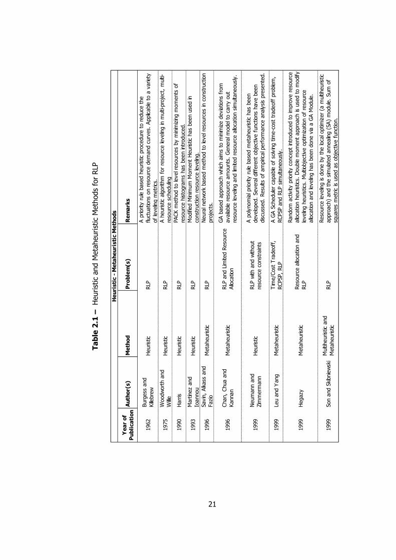
A summary of the heuristic and metaheuristic based methods mentioned in

this section is to be seen in Table 2.1 in a chronological order. Remarkable

points of each study have been given in addition to the information on the

methods adopted and problems addressed.

21

Year of

PublicationAuthor(s)

Method

Problem(s)

Remarks

1962

Burgess and

Killebrew

Heuristic

RLP

A priority rule based heuristic procedure to reduce the

fluctuations on resource demand curves. Applicable to a variety

of leveling m

etrics.

1975

Woodworth and

Willie

Heuristic

RLP

A heuristic algorithm for resource leveling in m

ulti-project, multi-

resource scheduling

1990

Harris

Heuristic

RLP

PACK m

ethod to level resources by m

inimizing m

oments of

resource histograms has been introduced.

1993

Martinez and

Ioannou

Heuristic

RLP

Modified M

inimum M

oment Heuristic has been used in

construction resource leveling.

1996

Savin, Alkass and

Fazio

Metaheuristic

RLP

Neural network based m

ethod to level resources in construction

projects.

1996

Chan, Chua and

Kannan

Metaheuristic

RLP and Limited Resource

Allocation

GA based approach which aims to m

inimize deviations from

available resource amounts. General m

odel to carry out

resource leveling and limited resource allocation simultaneously.

1999

Neumann and

Zimmerm

ann

Heuristic

RLP with and without

resource constraints

A polynomial priority rule based m

etaheuristic has been

developed. Several different objective functions have been

discussed. Results of ampirical perform

ance analysis presented.

1999

Leu and Yang

Metaheuristic

Time/Cost Tradeoff,

RCPSP, RLP

A GA Scheduler capable of solving time-cost tradeoff problem,

RCPSP and RLP simultaneously.

1999

Hegazy

Metaheuristic

Resource allocation and

RLP

Random activity priority concept introduced to im

prove resource

allocation heuristics. Double m

oment approach is used to m

odify

leveling heuristics. M

ultiobjective optim

ization of resource

allocation and leveling has been done via a GA M

odule.

1999

Son and Skibniewski

Multiheuristic and

Metaheuristic

RLP

Resource leveling is done by the local optim

izer (a m

ultiheuristic

approach) and the simulated annealing (SA) module. Sum of

squares metric is used as objective function.

Heuristic - Metaheuristic Methods

Table 2.1 – Heuristic and Metaheuristic Methods for RLP

22

Year of


Method

Problem(s)

Remarks

2000

Leu, Yang and

Huang

GA

RLP

Minimizes the absolute difference between the actual resource

usage and the uniform

resource usage. GA based system which

includes a DSS to enable planners consider several scenarios.

2000

Hiyassat

Heuristic

RLP

Different from Harris's M

ethod in selecting the activity to be

shifted. Less computation effort required to obtain as good as

or nearly as good as results compared to the traditional

method.

2001

Hiyassat

Heuristic

RLP

Modified M

inimum M

oment Approach is used to level resources

in m

ultiple resource projects.

2003

Oral,Laptalı Oral,

Bozkurt and Erdiş

Metaheuristic

RLP

A GA based resource leveling m

odule has been developed.

Deviations from uniform

resource usage is m

inimized.

2003

Zheng, Ng and

Kumarasw

amy

Metaheuristic

RLP

Multiobjective, GA based technique for optim

izing m

ultiresource

leveling problem. Promising results for medium and large sized

projects.

2004

Senouci and Eldin

Metaheuristic

RLP and RCPSP

simultaneously

A GA based m

ethod which has a wholistic approach towards PS

problems. It simultaneously deals with RLP and RCPSP.

2008

Pang, Shi and You

Metaheuristic

RLP

Single Resource Leveling using PSO with constriction factor. A

nine activity schedule has been presented as a case study.

2009

Guo, Li and Ye

PSO

RLP

PSO based m

ethod to level m

ultiple resources in multiple

projects.

2009

El-Rayes and Jun

GA

RLP

Two new leveling m

etrics; Release and Rehire and Resource Idle

Days defined. A GA M

odule to solve RLP using these new

metrics has been developed.

2010

Christodoulou, Ellinas

and Kamenou

Heuristic

RLP

Minimum M

oment Method using Entropy M

aximization has been

introduced. Activity stretching and compressing allowed for

better leveling.

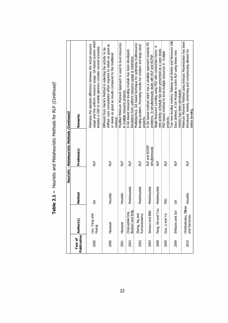
Heuristic - Metaheuristic Methods (Continued)

Table 2.1 – Heuristic and Metaheuristic Methods for RLP (Continued)

23

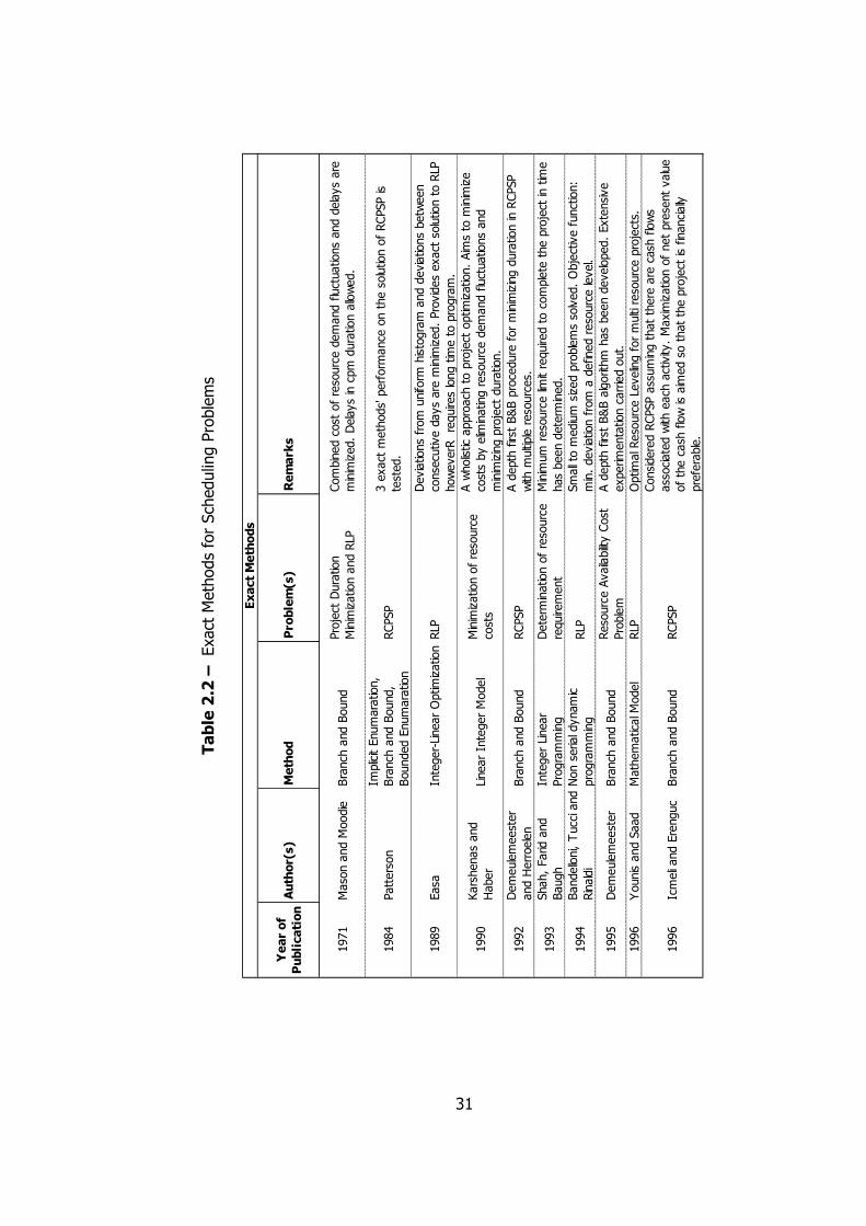
2.3 Exact Methods for RLP and Other Scheduling

Problems

In this section exact methods previously applied on RLP are going to be

discussed. Since there are limited number of branch and bound applications

developed for RLP, some branch and bound based studies for other

scheduling problems are also going to be mentioned.

One of the earliest branch and bound algorithms developed for project

scheduling problems is seen on Mason and Moodie (1971). In this study,

minimization of the combined cost of resource demand and delays in project

completion has been aimed to be minimized. Extensions in project duration

have been allowed and penalized according to a cost function. Also a penalty

function was applied if total resource amounts required by activities exceeded

available resource levels. The importance of lower bound calculations in

constructing a bounded decision tree has been emphasized and details of cost

bound calculations have been presented. While establishing the search tree,

activities that could be scheduled at that particular instance of time have been

considered and corresponding lower bounds have been calculated according

to possible scenarios. As branch and bound methodology implies, whether a

node is going to be discarded or retained has been decided according to the

lower bound value of that node. Also, resource constraints have been imposed

by eliminating any scenarios that require higher amounts of resources than

the available limits. 25 network problems have been solved to investigate the

performance of the algorithm and total number of nodes needed to ensure

optimality has been reported. It has been indicated that the computation time

is significantly related to factors such as number of activities and their

durations and resource requirements, in addition to the structure of the

project network. Developed algorithm has been declared to be helpful in

testing the performances of new heuristics (Mason and Moodie, 1971).

24

Patterson (1984) compared performances of three exact solution procedures

on RCPSP each of which were enumerative based and each of which tried to

eliminate non promising regions of the search space by utilizing special rules.

These three methods; bounded enumeration, branch and bound and implicit

enumeration have been tested on 110 problems in an imposed time limit of 5

minutes. Of these, only branch and bound algorithm was able to solve all

problems within the allowed time limit. According to the results reported,

implicit enumeration method required far less computer storage compared to

other two methods and bounded elimination method promised shortest

computation times for some instances. Despite these advantages of implicit

enumeration and bounded elimination, Patterson (1984) concluded that

branch and bound algorithm was likely to be the preferred method since it

allowed the search to be directed towards attractive solutions in the early

stages.

One of the earliest attempts to reduce resource level fluctuations in

construction projects using exact methods has been done by Easa (1989). In

this paper, an integer-linear optimization model to solve RLP optimally in small

to medium-sized networks has been introduced. This model guaranteed

optimal leveling by minimizing absolute deviations from a uniform resource

level. Also an improved objective function which minimized resource level

fluctuations in consecutive time periods has been suggested. Developed

optimization model has been tested on a sample network and optimal

resource histograms have been compared to the resource distribution of the

early start schedule. One drawback of the model was outlined as the need for

a high number of variables and constraints which made implementation of

integer-linear optimization difficult for most practical purposes (Easa, 1989).

Another linear integer optimization technique to minimize the sum of costs of

all resources, including time, has been presented by Karshenas and Haber

(1990). Two simple example projects’ costs have been minimized to illustrate

the performance of the model. It has been declared that the schedules

25

obtained from the model had an optimal duration and the resource use was

leveled economically. It has been indicated that a computer program is

needed to input the extensive data required to optimize the cost of a real life

example via the linear integer model (Karshenas and Haber, 1990).

Demeulemeester and Herroelen (1992) presented a branch and bound

procedure which adopted a depth-first methodology to solve RLP. Suggested

algorithm has been reported to be faster than the most rapid tools developed

so far and to be advantageous over them in that it required less computer

storage. In the introduced model, nodes have been constructed in a manner

that partial schedules, which were feasible both in terms of precedence

relations and resource limitations, were coded in them. At any time instant,

eligible activities that eligible to be scheduled have been considered and

nodes with higher lower bounds have been fathomed according to the

bounding rules. 110 test instances of Patterson (1984) have been employed to

validate the algorithm. It has been reported that the branch and bound

procedure presented in this study solved all instances successfully in an

average CPU time of 0.215 seconds per problem. Success of the method has

been attributed to the new bounding arguments and dominance rules

(Demeulemeester and Herroelen, 1992). Following this study, Shah, Farid and

Baugh (1993) introduced an integer linear optimization model which

determined minimum amount of resources required to complete a project.

Also, a non serial dynamic programming model to minimize absolute

deviations from a predefined resource level has been developed by Bandelloni,

Tucci and Rinaldi (1994).

Demeulemeester (1995) also addressed resource availability cost problem

which aims the determination of resource availability levels to minimize the

sum of availability costs. A branch and bound method, which was the first

exact method developed for this problem so far, was suggested for this

purpose. Computational experiments have been conducted on a small bridge

project in addition to the adapted problem set of Patterson (1984). Also,

26

effects of increasing resource types on the required computational efforts

have been observed. It has been reported that utilizing more resource types

causes the number of efficient points to increase, causing more considerations

during the search. Thus the standard computation time is declared to be an

increasing function of the number of resource types (Demeulemeester, 1995).

Among the exact solution procedures for scheduling problems, mathematical

model of Younis and Saad (1996) to carry out optimum resource leveling and

study of Icmeli and Erenguc (1996) to solve resource constrained project

scheduling problem with discounted cash flows (RCPSPDC) are also worth to

be mentioned. In the latter study, Icmeli and Erenguc (1996) developed a

depth first branch and bound algorithm which included a complete schedule

(whether feasible or not) in each node of the search tree. Branching was done

according to the “minimal delaying alternatives” concept of Demeulemeester

and Herroelen (1992). Developed model has been verified on an example and

experimentations have been done on a set of 90 test problems. It has been

indicated that the obtained results proved that the algorithm outperformed

other methods suggested to solve RCPSPDC so far (Icmeli and Erenguc,

1996).

Another depth-first branch and bound method has been developed by

Demeulemeester and Herroelen (1997) to solve the generalized RCPSP. This

algorithm which was an extension of the method formerly suggested by the

same researchers was able to represent any type of precedence relations such

as start to start, finish to finish etc. Partial feasible schedules have been

stored in the nodes of the search tree. Precedence based lower bound

calculations have been employed in addition to several dominance rules in

order to prune the search tree as much as possible. Extensive experimentation

has been conducted on Patterson’s problem set in order to compare the

impact of their modified search strategy and to study the impact of fluctuating

resource availabilities over time. It has been reported that 109 of 110 test

problems have been solved via the algorithm in an average CPU time of

27

8.1065 seconds. Demeulemeester and Herroelen (1997) concluded that the

computational experience gained with the modified algorithm was promising.

Examples of linear scheduling applications are to be seen in many construction

projects which require repetitive execution of tasks such as road projects, high

rise building constructions, pipeline constructions etc. Mattila and Abraham

(1998) were two of the few researchers who addressed RLP on linear

schedules. The integer linear programming model suggested by Mattila and

Abraham (1998) utilized an objective function to minimize the absolute

deviation of daily resource usage from an average resource rate. Resource

distribution of a highway project has been leveled using linear programming

software, LINDO. Resulting resource histogram has been presented in the

paper. Similar to most researchers who dealt with integer linear programming,

Mattila and Abraham (1998) also indicated that a high number of variables

were required by this method which limited the size of the problem that could

effectively be dealt.

Brucker et al. (1998) presented another branch and bound method addressing

RCPSP. This study differed from similar methods in that it included a tabu

search procedure in the root of the search tree to begin the search with a

better schedule. Moreover, a linear program based lower bound calculation

procedure has been employed on each node. Experimentations have been

carried out on networks of 30 and 60 activities and with 4 resource types. It

has been declared that 326 of 480 test problems with 60 activities have been

solved to optimality within one hour (Brucker et al., 1998). Following this

study, De Reyck and Herroelen (1998) published a paper in which they

presented another depth first branch and bound algorithm for RCPSP with

generalized precedence relations. Nodes of the search tree represented a time

feasible solution for the problem which was not necessarily resource feasible.

To overcome this resource conflict, the method of “minimal delaying

alternatives” has been employed. Details of a new lower bound calculation

procedure and three dominance rules have been presented. Extensive

28

experimentation results on three different data sets have been reported and it

has been indicated that the suggested algorithm enabled significant reductions

in the computation time. Moreover, RCPSP has been solved to optimality for

networks with up to 100 activities (De Reyck and Herroelen, 1998).

Neumann and Zimmermann (2000) published a paper in which different

heuristic and exact procedures have been proposed in order to solve RLP and

net present value problem. In this study RLP has been investigated under

three main categories which are; minimization of costs due resource level

fluctuations (resource investment problem), minimization of deviations from a

given resource level and minimization of fluctuations in consecutive time

periods. These objective functions and some variations of them have been

utilized to level resources in networks with and without resource limitations.

Similarly, net present value problem with and without resource constraints has

been addressed via exact methods. To solve resource leveling problems,

branch and bound and truncated branch and bound procedures have been

employed (Neumann and Zimmermann, 2000).

Branch and bound procedure developed by Neumann and Zimmermann

(2000) was based on an enumeration of feasible start times of activities and

each node of the tree represented a partial schedule. Consequently, each leaf,

i.e. the deepest nodes on the tree, represented a complete schedule. Children

of nodes have been obtained by scheduling one of the eligible activities to a

starting date that is feasible. If multiple activities were available to be

scheduled, than the one with the lowest total float was selected. Naturally, the

node from which children are to be produced was selected according to a

minimum lower bound criterion. In the truncated branch and bound

procedure, on the other hand, a heuristic has filtered the number of branches

to be produced from a single node. In other words, only a certain number of

most promising branches have been allowed to grow (Neumann and

Zimmermann, 2000).

29

Neumann and Zimmermann (2000) also presented a tabu search approach for

RLP and reported extensive experimentation via the abovementioned exact

and heuristic approaches. Three problem sets which included a number of

networks with 10 to 500 activities and with 1 to 5 different types of resources

have been used in experimentation. It has been reported that resource

constraints significantly reduced size of the feasible regions of the search tree

causing the algorithms to locate optimal solutions in shorter durations. Most

problem instances consisting of up to 20 activities have been solved by the

developed branch and bound procedures in less than 100 seconds. It has

been declared that networks with 20 activities and five resources have been

solved to optimality for the first time in the literature. A need for tighter lower

bound calculations for different resource leveling metrics has been indicated

(Neumann and Zimmermann, 2000).

Another branch and bound algorithm has been introduced by Vanhoucke,

Demeulemeester and Herroelen (2001). Maximization of the net present value

has been aimed in this study. New upper bound computation methods and an

extended branching strategy to prune the search tree considerably have been

introduced. Experimentations have been conducted on the problem sets of

Patterson (1984) and Icmeli and Erenguc (1996). It has been indicated that

net present value problem has been solved to optimality for networks with up

to 30 activities and 4 resource types (Vanhoucke, Demeulemeester and

Herroelen, 2001).

In project scheduling literature, one of the most common assumptions is that

an activity can not be stopped and can not be restarted. Son and Mattila

(2004) indicated that this assumption may not always be true in construction

industry since some activities in construction projects can actually be splitted.

To carry out a more realistic optimization, a linear program binary variable

model to level resources that permits selected activities to stop and restart

has been introduced. This model included constraints on daily resource rates.

Moreover, total duration of activities, whether they are splitted or not was

30

fixed. Son and Mattila (2004) solved two example projects and reported that

the developed model was capable of representing actual construction

processes successfully.

One of the most recent exact procedures to solve RCPSP was developed by

Jiang and Shi (2005). This method, “enumerative branch and cut procedure”,

included a cut rule to eliminate true worse schedule alternatives as done in

the truncated branch and bound procedure of Neumann and

Zimmermann (2000). It has been reported that 110 test problems in

Patterson’s set could be solved via the developed algorithm in a reasonable

amount of time. Jiang and Shi (2005) indicated that computational efficiency

should not be a big concern while solving scheduling problems, since

scheduling is not repeated over and over during the lifecycle of projects.

Similar to Table 2.1, which presented heuristic and metaheuristic methods

developed to solve RLP, Table 2.2 summarizes exact methods for scheduling

problems in a chronological order. Problems addressed in these studies,

methods developed and remarks have been highlighted.

31

Year of


Method

Problem(s)

Remarks

1971

Mason and M

oodie

Branch and Bound

Project Duration

Minimization and RLP

Combined cost of resource demand fluctuations and delays are

minimized. Delays in cpm duration allowed.

1984

Patterson

Implicit Enumaration,

Branch and Bound,

Bounded Enumaration

RCPSP

3 exact m

ethods' perform

ance on the solution of RCPSP is

tested.

1989

Easa

Integer-Linear Optim

izationRLP

Deviations from uniform

histogram and deviations between

consecutive days are m

inimized. Provides exact solution to RLP

howeverR requires long time to program.

1990

Karshenas and

Haber

Linear Integer Model

Minimization of resource

costs

A wholistic approach to project optim

ization. Aims to m

inimize

costs by elim

inating resource demand fluctuations and

minimizing project duration.

1992

Demeulemeester

and Herroelen

Branch and Bound

RCPSP

A depth first B&B procedure for minimizing duration in RCPSP

with m

ultiple resources.

1993

Shah, Farid and

Baugh

Integer Linear

Programming

Determ

ination of resource

requirement

Minimum resource limit required to complete the project in time

has been determ

ined.

1994

Bandelloni, Tucci and

Rinaldi

Non serial dynamic

programming

RLP

Small to m

edium sized problems solved. Objective function:

min. deviation from a defined resource level.

1995

Demeulemeester

Branch and Bound

Resource Availability Cost

Problem

A depth first B&B algorithm has been developed. Extensive

experim

entation carried out.

1996

Younis and Saad

Mathematical M

odel

RLP

Optim

al Resource Leveling for multi resource projects.

1996

Icmeli and Erenguc

Branch and Bound

RCPSP

Considered RCPSP assuming that there are cash flows

associated with each activity. Maximization of net present value

of the cash flow is aimed so that the project is financially

preferable.

Exact Methods

Table 2.2 – Exact Methods for Scheduling Problems

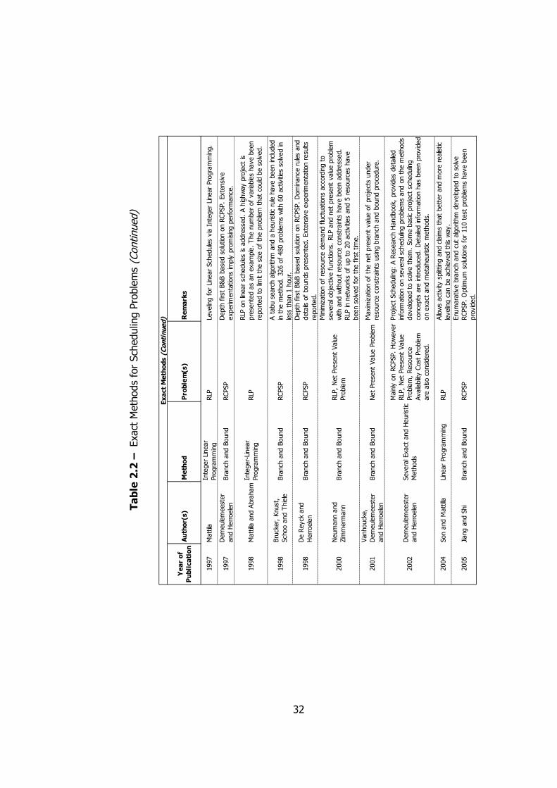
32

Year of


Method

Problem(s)

Remarks

1997

Mattila

Integer Linear

Programming

RLP

Leveling for Linear Schedules via Integer Linear Programming.

1997

Demeulemeester

and Herroelen

Branch and Bound

RCPSP

Depth first B&B based solution on RCPSP. Extensive

experim

entations imply promising perform

ance.

1998

Mattilla and Abraham

Integer-Linear

Programming

RLP

RLP on linear schedules is addressed. A highway project is

presented as an example. The number of variables have been

reported to limit the size of the problem that could be solved.

1998

Brucker, Knust,

Schoo and Thiele

Branch and Bound

RCPSP

A tabu search algorithm and a heuristic rule have been included

in the m

ethod. 326 of 480 problems with 60 activities solved in

less than 1 hour.

1998

De Reyck and

Herroelen

Branch and Bound

RCPSP

Depth first B&B based solution on RCPSP. Dominance rules and

details of bounds presented. Extensive experim

entation results

reported.

2000

Neumann and

Zimmerm

ann

Branch and Bound

RLP, Net Present Value

Problem

Minimization of resource demand fluctuations according to

several objective functions. RLP and net present value problem

with and without resource constraints have been addressed.

RLP in networks of up to 20 activities and 5 resources have

been solved for the first tim

e.

2001

Vanhoucke,

Demeulemeester

and Herroelen

Branch and Bound

Net Present Value Problem

Maximization of the net present value of projects under

resource constraints using branch and bound procedure.

2002

Demeulemeester

and Herroelen

Several Exact and Heuristic

Methods

Mainly on RCPSP. However

RLP, Net Present Value

Problem, Resource

Availability Cost Problem

are also considered.

Project Scheduling: A Research Handbook, provides detailed

inform

ation on several scheduling problems and on the m

ethods

developed to solve them. Some basic project scheduling

concepts are introduced. Detailed inform

ation has been provided

on exact and m

etaheuristic m

ethods.

2004

Son and M

attilla

Linear Programming

RLP

Allows activity splitting and claims that better and m

ore realistic

leveling can be achieved this way.

2005

Jiang and Shi

Branch and Bound

RCPSP

Enumarative branch and cut algorithm developed to solve

RCPSP. Optim

um solutions for 110 test problems have been

provided.

Exact Methods (Continued)

Table 2.2 – Exact Methods for Scheduling Problems (Continued)

33

Considering the literature on exact methods for solving RLP, it can be said

that the number of studies effectively dealing with the problem is highly

limited. Especially, resource distributions of construction projects have seldom

been leveled to optimality. In attempts to solve RLP via optimization methods

as integer linear optimization, several researchers declared that these efforts

required high number of variables to be defined which in some problems even

exceeded the limitations of commercial software. Often, branch and bound

method has been pointed out as the most effective exact method in dealing

with RLP.

Another important aspect while solving RLP in construction projects is related

to the objective functions employed by researchers. Some resource leveling

metrics, such as minimum absolute deviations from uniform resource level,

are being used by many researchers in construction project scheduling. This

situation implies useless efforts since the rectangular resource distribution

graph aimed in this kind of metrics is not suitable for the construction

projects.

In the following chapter, characteristics of the branch and bound method

developed to level resources in construction projects using suitable objective

functions to the nature of the construction business are going to be

presented.

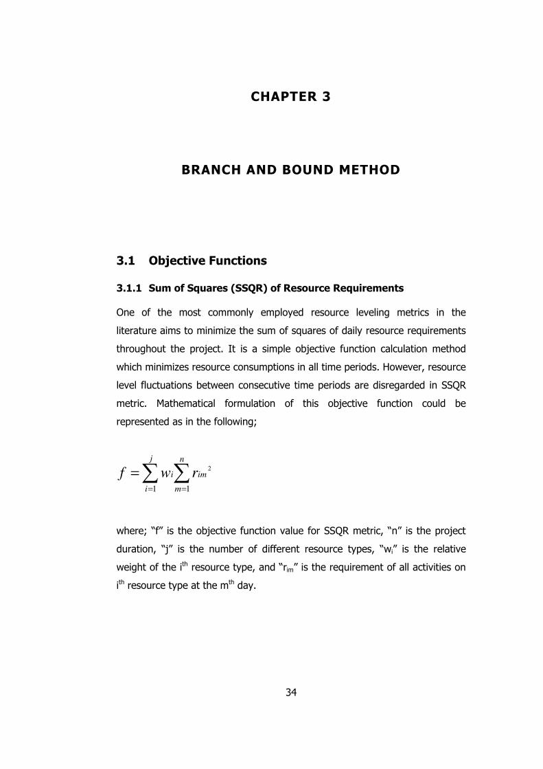
34

CHAPTER 3

BRANCH AND BOUND METHOD

3.1 Objective Functions

3.1.1 Sum of Squares (SSQR) of Resource Requirements

One of the most commonly employed resource leveling metrics in the

literature aims to minimize the sum of squares of daily resource requirements

throughout the project. It is a simple objective function calculation method

which minimizes resource consumptions in all time periods. However, resource

level fluctuations between consecutive time periods are disregarded in SSQR

metric. Mathematical formulation of this objective function could be

represented as in the following;

where; “f” is the objective function value for SSQR metric, “n” is the project

duration, “j” is the number of different resource types, “wi” is the relative

weight of the ith resource type, and “rim” is the requirement of all activities on

ith resource type at the mth day.

∑∑==

=n

m

im

j

i

i rwf11

2

35

5

4

3

2

1

0

1 2 3 4 5 6Days

Resource Requirements

Figure 3.1 – Sample Resource Distribution

A sample 6 days project is given in Figure 3.1 to be used in illustrating the

metrics presented in this section. If the resource distribution on this figure is

considered, then the SSQR value of the project is simply to be calculated as in

the following;

SSQR = 52 + 32 + 22 + 42 + 22 + 32 = 67

3.1.2 Minimum Absolute Deviation (MinDev) of Resource

Requirements from Uniform Resource Level

Another commonly employed objective function firstly calculates the uniform

resource level required to complete the project and then minimizes absolute

deviations from this level. To calculate this uniform resource level, total

amount of resources required to complete the project is divided to the project

duration and obtained number is rounded down to the closest integer. This

metric aims to obtain a rectangle shaped resource distribution, suitability of

which to construction projects is questionable. Still, MinDev metric has been

36

used in our study to validate the developed algorithm by comparing our

optimal solutions to the results reported in previous studies. Mathematical

representation of MinDev objective function may be defined as in the

following;

Where;

And where; “f” is the objective function value for MinDev metric, “n” is the

project duration, “j” is the number of different resource types, “wi” is the

relative weight of the ith resource type and “rim” is the requirement of all

activities on ith resource type at the mth day. In addition to these, “ui”

represents uniform resource level, “y” is the total number of activities, “demxi”

is the total demand of activity x on resource type i and durx is the duration of

activity x. “⌊…⌋” notation used in calculation of ui symbols the floor function

which rounds a decimal to the closest integer smaller than or equal to that

decimal.

According to this metric, objective function value of the resource distribution

in Figure 3.1 is calculated as in the following;

ui = ⌊ (5 + 3 + 2 + 4 + 2 + 3) / 6 ⌋ = 3

Dev= |5 - 3| + |3 - 3| + |2 - 3| + |4 - 3| + |2 - 3| + |3 - 3| = 5

∑∑==

−=n

m

imi

j

i

i ruwf11

×

=

∑=

n

durdem

u

y

x

xxi

i1

37

3.1.3 Resource Idle Days (RID)

As mentioned in Chapter 2, El-Rayes and Jun (2009) suggested a resource

leveling metric which is especially useful if resources can not be released and

rehired easily throughout the makespan of a project. In other words, RID

metric which minimizes idle times of resources without forcing the resource

distribution to fit a predefined shape has been established by the researchers.

Mathematical formulation of the metric defined by El-Rayes and Jun (2009)

might be modified to level multiple resources as in the following;

Where; “n” is the project duration, “j” is the number of different resource

types, “wi” is the relative weight of the ith resource type and “rim” is the

requirement of all activities on ith resource type at the mth day.

Again, considering the resource distribution in Figure 3.1;

RID = [Min (5, 5) - 5] + [Min (5, 4) - 3] + [Min (5, 4) - 2] +

[Min (5, 4) - 4] + [Min (5, 3) - 2] + [Min (5, 3) - 3] = 4

If Figure 3.2 is considered, these 4 units of idle resources are seen on the

hatched zones of the profile. RID metric aims to minimize these zones which

indicate unproductive resource days. As can be realized, RID metric focuses

on minimizing the undesirable fluctuations only, whereas most traditional

metrics attempt to transform resource profiles to predetermined shapes (El-

Rayes and Jun, 2009). Hence RID can handle RLP in a more flexible way

resulting in more efficient resource distributions.

[ ]∑=

−∑=

= +

n

mrrrrMaxrrrMaxMin

j

iwf iminimimimiii

1)),...,,(),,...,,((

1121

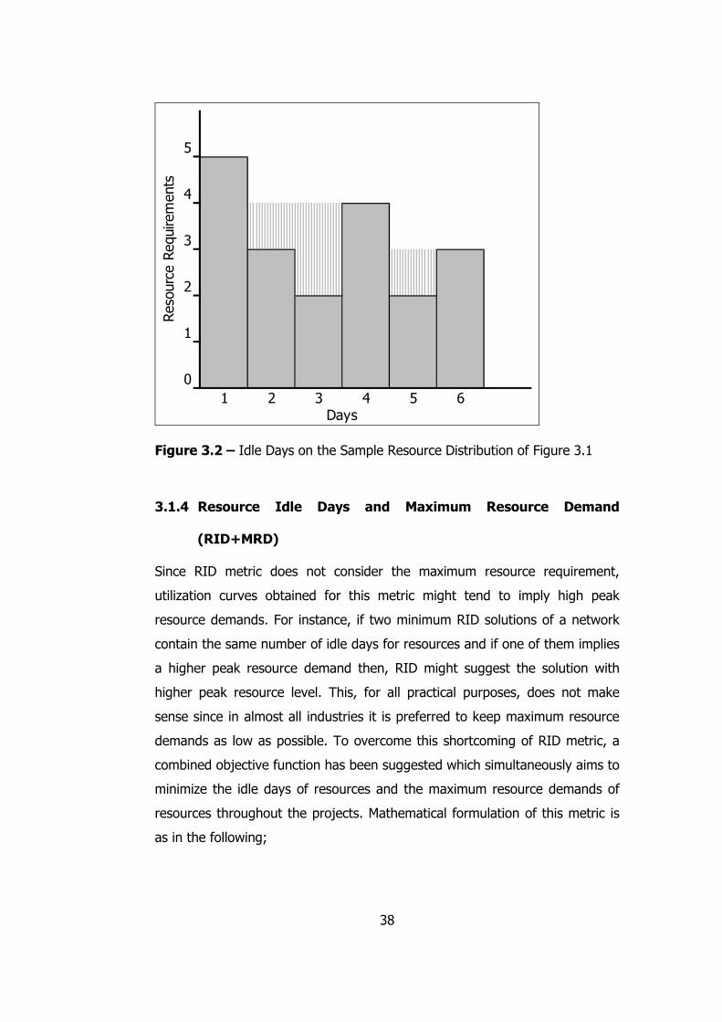
38

5

4

3

2

1

0

1 2 3 4 5 6Days


Figure 3.2 – Idle Days on the Sample Resource Distribution of Figure 3.1

3.1.4 Resource Idle Days and Maximum Resource Demand

(RID+MRD)

Since RID metric does not consider the maximum resource requirement,

utilization curves obtained for this metric might tend to imply high peak

resource demands. For instance, if two minimum RID solutions of a network

contain the same number of idle days for resources and if one of them implies

a higher peak resource demand then, RID might suggest the solution with

higher peak resource level. This, for all practical purposes, does not make

sense since in almost all industries it is preferred to keep maximum resource

demands as low as possible. To overcome this shortcoming of RID metric, a

combined objective function has been suggested which simultaneously aims to

minimize the idle days of resources and the maximum resource demands of

resources throughout the projects. Mathematical formulation of this metric is

as in the following;

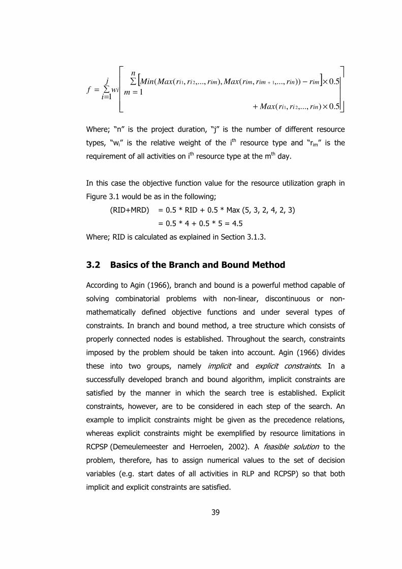
39

Where; “n” is the project duration, “j” is the number of different resource

types, “wi” is the relative weight of the ith resource type and “rim” is the

requirement of all activities on ith resource type at the mth day.

In this case the objective function value for the resource utilization graph in

Figure 3.1 would be as in the following;

(RID+MRD) = 0.5 * RID + 0.5 * Max (5, 3, 2, 4, 2, 3)

= 0.5 * 4 + 0.5 * 5 = 4.5

Where; RID is calculated as explained in Section 3.1.3.

3.2 Basics of the Branch and Bound Method

According to Agin (1966), branch and bound is a powerful method capable of

solving combinatorial problems with non-linear, discontinuous or non-

mathematically defined objective functions and under several types of

constraints. In branch and bound method, a tree structure which consists of

properly connected nodes is established. Throughout the search, constraints

imposed by the problem should be taken into account. Agin (1966) divides

these into two groups, namely implicit and explicit constraints. In a

successfully developed branch and bound algorithm, implicit constraints are

satisfied by the manner in which the search tree is established. Explicit

constraints, however, are to be considered in each step of the search. An

example to implicit constraints might be given as the precedence relations,

whereas explicit constraints might be exemplified by resource limitations in

RCPSP (Demeulemeester and Herroelen, 2002). A feasible solution to the

problem, therefore, has to assign numerical values to the set of decision

variables (e.g. start dates of all activities in RLP and RCPSP) so that both

implicit and explicit constraints are satisfied.

[ ]

×+

×∑=

−∑=

=+

5.0),...,,(

5.0

1

)),...,,(),,...,,((

1

21

121

inii

iminimimimii

i

rrrMax

n

m

rrrrMaxrrrMaxMinj

iwf

40

Nodes, of which a search tree consists of, are subsets of the set of all

solutions of the combinatorial problem. Branching, on the other hand, is the

partitioning of any set of feasible solutions into separate subsets (Agin, 1966).

Branching process starts from the root node (the node in the uppermost level

of the tree) which represents the set of all solutions. In some instances during

the search there might be nodes from which no branching has occurred yet.

These nodes which are to be discovered further are called intermediate nodes.

On the contrary to intermediate nodes which imply a partial solution, final

nodes represent a complete solution. In order to reach a final node (leaf), all

decisions required to establish a valid solution set have to be made. In RLP,

for example, a leaf stores start dates of all non critical activities. Obviously

final nodes are located in the lowermost level of the search tree.

Two main characteristics of branch and bound algorithms presented by Agin

(1966) are branching characteristic and bounding characteristic. According to

the definitions provided, branching characteristic ensures that an optimal

solution is going to be reached at the end of the search since all possible

combinations are going to be considered. Whereas, bounding characteristic

implies a possibility to reach the optimal solution without visiting each node by

pruning some parts of the tree.

Finally definition of lower bound should be given since this concept is in the

very heart of the branch and bound logic. Lower bound is a value of the

objective function for all solutions included in a specific node such that none

of the solutions that could be branched from that node will have a better

objective function value than that bound. As this definition implies, there is no

use to branch a node any further if its lower bound value is worse than the

objective function value of one of the explored final nodes (complete

solutions). Objective function value of the best complete solution explored so

far, i.e. upper bound, is used to decide whether a node is promising or not.

Obviously, upper bound at the end of the search provides the optimal solution

to the problem.

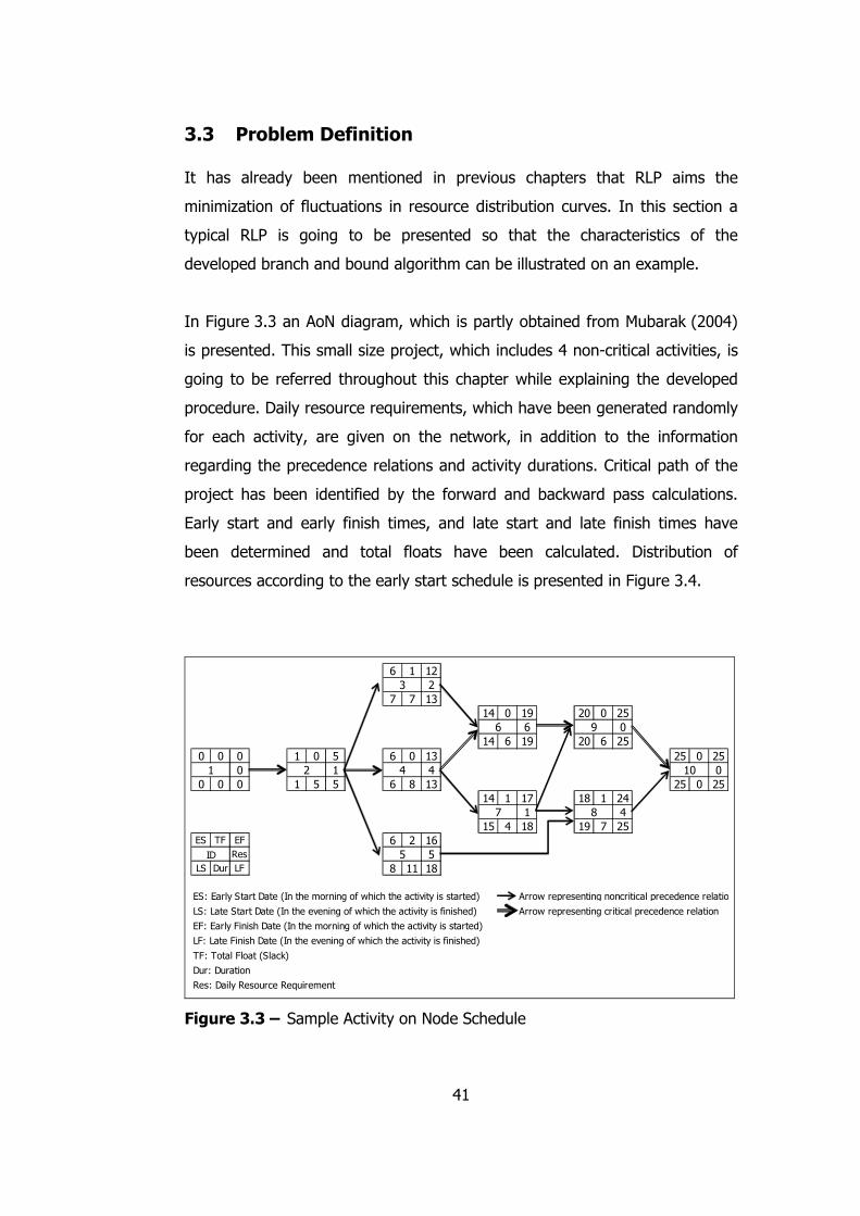
41

3.3 Problem Definition

It has already been mentioned in previous chapters that RLP aims the

minimization of fluctuations in resource distribution curves. In this section a

typical RLP is going to be presented so that the characteristics of the

developed branch and bound algorithm can be illustrated on an example.

In Figure 3.3 an AoN diagram, which is partly obtained from Mubarak (2004)

is presented. This small size project, which includes 4 non-critical activities, is

going to be referred throughout this chapter while explaining the developed

procedure. Daily resource requirements, which have been generated randomly

for each activity, are given on the network, in addition to the information

regarding the precedence relations and activity durations. Critical path of the

project has been identified by the forward and backward pass calculations.

Early start and early finish times, and late start and late finish times have

been determined and total floats have been calculated. Distribution of

resources according to the early start schedule is presented in Figure 3.4.

6 1 12

2

7 7 13

14 0 19 20 0 25

6 0

14 6 19 20 6 25

0 0 0 1 0 5 6 0 13 25 0 25

0 1 4 0

0 0 0 1 5 5 6 8 13 25 0 25

14 1 17 18 1 24

1 4

15 4 18 19 7 25ES TF EF 6 2 16

Res 5LS Dur LF 8 11 18

ES: Early Start Date (In the morning of which the activity is started) Arrow representing noncritical precedence relation

LS: Late Start Date (In the evening of which the activity is finished) Arrow representing critical precedence relation

EF: Early Finish Date (In the morning of which the activity is started)

LF: Late Finish Date (In the evening of which the activity is finished)

TF: Total Float (Slack)

Dur: Duration

Res: Daily Resource Requirement

1 2 4

6

7

9

8

10

ID

3

5

Figure 3.3 – Sample Activity on Node Schedule

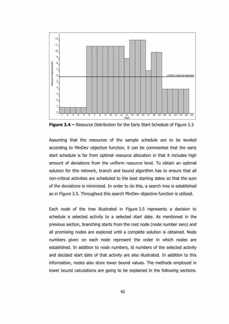
42

12

11

10

9

8

7

6 uniform resource demand

5

4

3

2

1

0

1 2 3 4 5 6 7 8 9 10 11 12 13 14 15 16 17 18 19 20 21 22 23 24 25Days


Figure 3.4 – Resource Distribution for the Early Start Schedule of Figure 3.3

Assuming that the resources of the sample schedule are to be leveled

according to MinDev objective function, it can be commented that the early

start schedule is far from optimal resource allocation in that it includes high

amount of deviations from the uniform resource level. To obtain an optimal

solution for this network, branch and bound algorithm has to ensure that all

non-critical activities are scheduled to the best starting dates so that the sum

of the deviations is minimized. In order to do this, a search tree is established

as in Figure 3.5. Throughout this search MinDev objective function is utilized.

Each node of the tree illustrated in Figure 3.5 represents a decision to

schedule a selected activity to a selected start date. As mentioned in the

previous section, branching starts from the root node (node number zero) and

all promising nodes are explored until a complete solution is obtained. Node

numbers given on each node represent the order in which nodes are

established. In addition to node numbers, id numbers of the selected activity

and decided start date of that activity are also illustrated. In addition to this

information, nodes also store lower bound values. The methods employed in

lower bound calculations are going to be explained in the following sections.

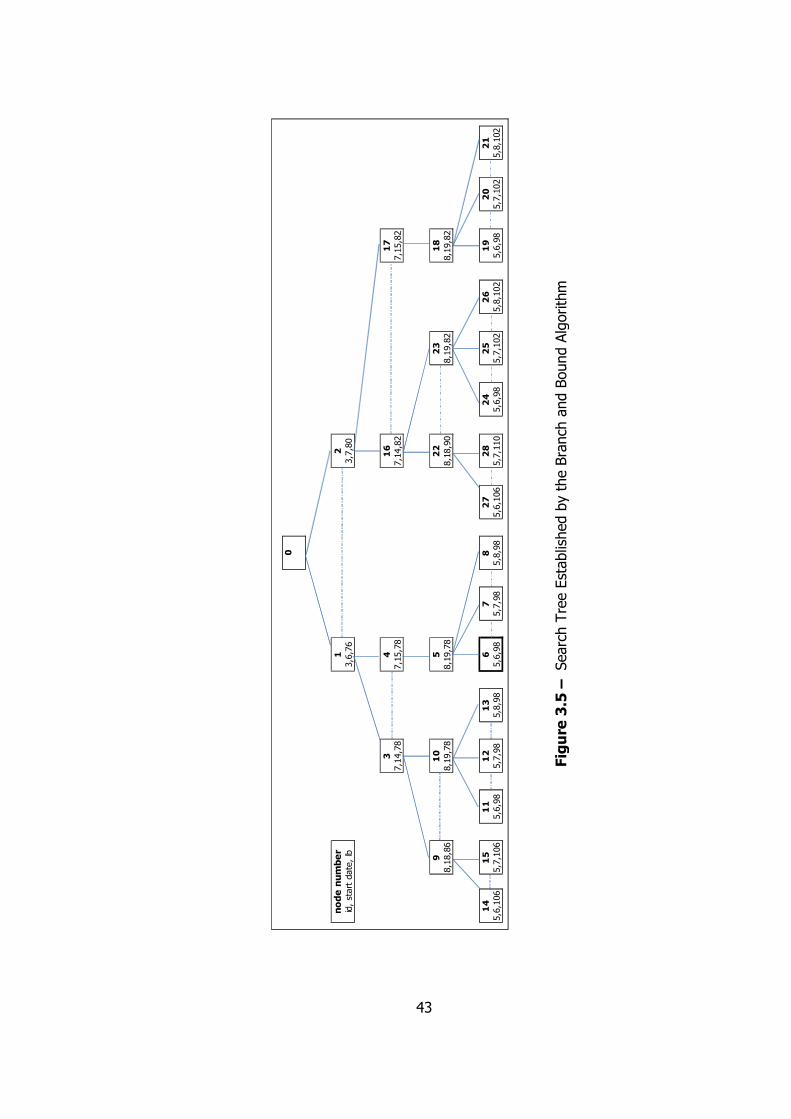
43

0

1

3,6,76

2

3,7,80

3

7,14,78

4

7,15,78

16

7,14,82

17

7,15,82

9

8,18,86

10

8,19,78

5

8,19,78

22

8,18,90

23

8,19,82

18

8,19,82

14

5,6,106

15

5,7,106

11

5,6,98

12

5,7,98

13

5,8,98

6

5,6,98

7

5,7,98

8

5,8,98

27

5,6,106

28

5,7,110

24

5,6,98

25

5,7,102

26

5,8,102

19

5,6,98

20

5,7,102

21

5,8,102

node number

id, start date, lb

Figure 3.5 – Search Tree Established by the Branch and Bound Algorithm

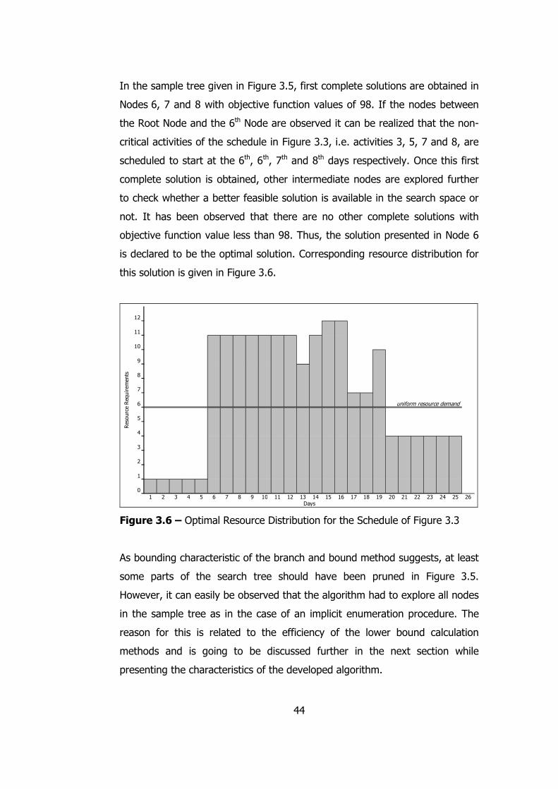
44

In the sample tree given in Figure 3.5, first complete solutions are obtained in

Nodes 6, 7 and 8 with objective function values of 98. If the nodes between

the Root Node and the 6th Node are observed it can be realized that the non-

critical activities of the schedule in Figure 3.3, i.e. activities 3, 5, 7 and 8, are

scheduled to start at the 6th, 6th, 7th and 8th days respectively. Once this first

complete solution is obtained, other intermediate nodes are explored further

to check whether a better feasible solution is available in the search space or

not. It has been observed that there are no other complete solutions with

objective function value less than 98. Thus, the solution presented in Node 6

is declared to be the optimal solution. Corresponding resource distribution for

this solution is given in Figure 3.6.

12

11

10

9

8

7

6 uniform resource demand

5

4

3

2

1

0

1 2 3 4 5 6 7 8 9 10 11 12 13 14 15 16 17 18 19 20 21 22 23 24 25 26


Days

Figure 3.6 – Optimal Resource Distribution for the Schedule of Figure 3.3

As bounding characteristic of the branch and bound method suggests, at least

some parts of the search tree should have been pruned in Figure 3.5.

However, it can easily be observed that the algorithm had to explore all nodes

in the sample tree as in the case of an implicit enumeration procedure. The

reason for this is related to the efficiency of the lower bound calculation

methods and is going to be discussed further in the next section while

presenting the characteristics of the developed algorithm.

45

According to Agin (1966), a branch and bound algorithm might be said to

consist of rules for;

1. deciding on how to continue the search given an intermediate

node (branching rule);

2. deciding on how to calculate lower bounds on each established node;

3. deciding on the intermediate node from which to branch next;

4. recognizing when a node contains only infeasible or non-optimal

solutions;

5. recognizing optimal solutions encountered on final nodes.

These rules are going to be employed as an outline while presenting the

characteristics of the developed algorithm.

3.4 Characteristics of the Developed Branch and Bound

Algorithm

In this section, characteristics of the suggested depth-first least-lower-bound

branch and bound procedure are going to be given. Developed algorithm

enumerates feasible start times of activities and can be applied to all metrics

presented in Section 3.1. It attempts to solve the RLP in traditional sense, i.e.

without any resource constraints. Details of the procedure are explained in

detail based on the schedule presented in Figure 3.3.

3.4.1 Branching from Nodes to New Nodes

Nodes in the developed algorithm store information about already sequenced

activities and start dates of these activities. In other words, each node

contains a partial feasible schedule and a list of unscheduled activities. In

each node one activity is scheduled to one of its start dates. While doing this,

feasibility of the partial or complete solutions is maintained by allowing only

feasible start dates of activities to be established. Number of activities that

need to be sequenced to reach a complete solution after a specific node is

equal to the number of unscheduled activities stored in that node.

46

Nodes branched directly from a node are the children of it. If there is more

than one children of a parent node then these are said to be brothers of each

other. In each parent node, one activity is selected to be scheduled in the

next step. It is the total float value of this activity that is used to decide on the

number of children of that node. In Figure 3.5 for example, Node 1 is the

parent of Node 3 and Node 4 which are brothers of each other. The reason

why Node 1 has only two children is due to the fact that Activity 7, which is

selected to be sequenced in the next step, has a total float value of one. Since

all possible start dates of a selected activity have to be represented on

different nodes, two nodes for Activity 7, one setting the start time to 14th day

and one to 15th day, have to be established. In other words, once an activity

is chosen to be scheduled, number of nodes established immediately is

“TF+1”. At this point it is important to note that the TF under consideration is

the updated TF value according to the previous decisions, rather than the one

defined in the early start schedule.

As the previous paragraph implies, to select the activity to be sequenced after

a node, feasible start dates and total floats of activities have to be

recalculated each time. Such an update is essential in order to consider the

effects of previously made decisions on the tree. To be more specific, since

there is a possibility that feasible start dates of a candidate activity might have

been changed due to formerly scheduled activities, possible early and late

start dates of all activities have to be determined again and again every time a

node has been established. The necessity of this can better be understood if

Node 5 on Figure 3.5 is considered. While introducing this node, Activity 8 has

been selected to be scheduled. If the AoN diagram in Figure 3.3 is examined,

this activity, which has a one day total float, should have two feasible start

times which are 18th and 19th days. However, checking the parent node it can

immediately be realized that Activity 7 which is a predecessor of Activity 8 has

been scheduled to day 15 which means that finish date of this activity can be

no earlier than 18th day. Thus Activity 8 is scheduled to its only possible start

date which is the 19th day.

47

3.4.2 Determining Lower Bounds for the New Nodes

Lower bound of each node is calculated by the algorithm in order to predict

the best objective function value that could be obtained at the end of the

search if that node is explored further. In other words, best scenario that

could occur after that point of the search is taken into the account. If the best

possible complete solution has an objective function value worse than or equal

to one of the known solutions so far, then that node is fathomed, i.e. not

explored any further. As emphasized earlier, lower bound calculations play an

important role in branch and bound methods since better (tighter) lower

bounds enable algorithms to prune more of the search space which results in

increased computational efficiency. In fact, the extent to which a smallest

improvement in lower bound calculations could reduce the required

computational effort might be highly significant in some cases. An example to

such an improvement and its effects on the search tree presented in

Figure 3.5 is going to be provided later in this section; however, initially some

information on the employed lower bound calculations is presented. First three

of these lower bound calculation methods have previously been suggested by

Neumann and Zimmermann (2000). The fourth one, however, is suggested

for the first time in this study.

3.4.2.1 – Discarding Critical Activities

Since RLP does not allow the makespan determined in early start schedule to

be extended, in our search none of the critical activities can be delayed.

Resources of these activities, however, have to be incorporated in the

resource utilization graphs in order to properly calculate the objective function

values. Therefore, fixed resources required by the critical activities are

determined and included to the resource distribution at the beginning of the

search and are taken into account during each lower bound determination.

Resource utilization graph for critical activities of the schedule presented in

Figure 3.3 is to be seen on Figure 3.7 (a).

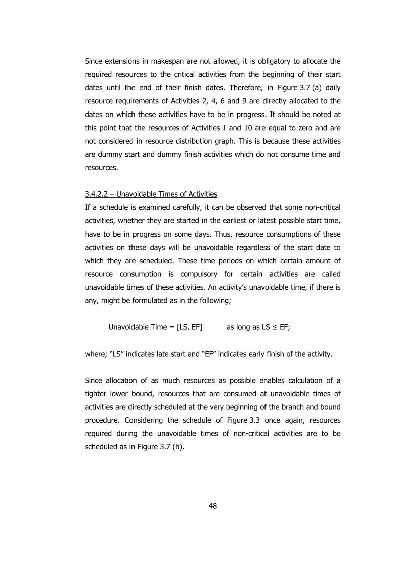
48

Since extensions in makespan are not allowed, it is obligatory to allocate the

required resources to the critical activities from the beginning of their start

dates until the end of their finish dates. Therefore, in Figure 3.7 (a) daily

resource requirements of Activities 2, 4, 6 and 9 are directly allocated to the

dates on which these activities have to be in progress. It should be noted at

this point that the resources of Activities 1 and 10 are equal to zero and are

not considered in resource distribution graph. This is because these activities

are dummy start and dummy finish activities which do not consume time and

resources.

3.4.2.2 – Unavoidable Times of Activities

If a schedule is examined carefully, it can be observed that some non-critical

activities, whether they are started in the earliest or latest possible start time,

have to be in progress on some days. Thus, resource consumptions of these

activities on these days will be unavoidable regardless of the start date to

which they are scheduled. These time periods on which certain amount of

resource consumption is compulsory for certain activities are called

unavoidable times of these activities. An activity’s unavoidable time, if there is

any, might be formulated as in the following;

Unavoidable Time = [LS, EF] as long as LS ≤ EF;

where; “LS” indicates late start and “EF” indicates early finish of the activity.

Since allocation of as much resources as possible enables calculation of a

tighter lower bound, resources that are consumed at unavoidable times of

activities are directly scheduled at the very beginning of the branch and bound

procedure. Considering the schedule of Figure 3.3 once again, resources

required during the unavoidable times of non-critical activities are to be

scheduled as in Figure 3.7 (b).

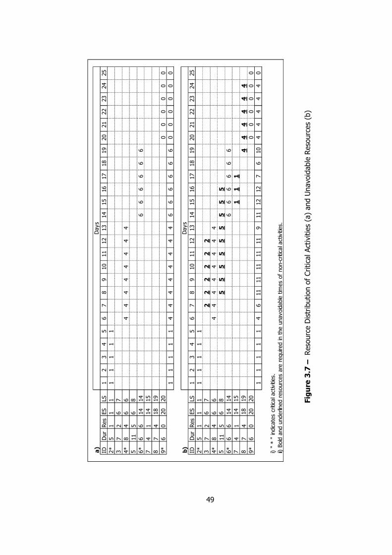
49

a)

IDDurRes

ES

LS1

23

45

67

89

10

11

12

13

14

15

16

17

18

19

20

21

22

23

24

25

2*

51

11

11

11

1

37

26

7

4*

84

66

44

44

44

44

511

56

8

6*

66

14

14

66

66

66

74

114

15

87

418

19

9*

60

20

20

00

00

00

11

11

14

44

44

44

46

66

66

60

00

00

0

b)

IDDurRes

ES

LS1

23

45

67

89

10

11

12

13

14

15

16

17

18

19

20

21

22

23

24

25

2*

51

11

11

11

1

37

26

72

22

22

24*

84

66

44

44

44

44

511

56

85

55

55

55

55

6*

66

14

14

66

66

66

74

114

15

11

18

74

18

19

44

44

44

9*

60

20

20

00

00

00

11

11

14

611

11

11

11

11

911

12

12

76

10

44

44

40

i) " * " indicates critical activities.

ii) Bold and underlined resources are required in the unavoidable times of non-critical activities.

Days

Days

Figure 3.7 – Resource Distribution of Critical Activities (a) and Unavoidable Resources (b)

50

In the sample network given in Figure 3.3, it can be observed that for all non-

critical activities the condition LS ≤ EF holds. This means that these activities

are going to be in progress in their unavoidable time periods. Considering

Activity 3, for example, unavoidable time period of this activity is the duration

between its late start and early finish times which are given as 7th and 12th

days. Therefore, daily resource requirement (2 units of resources/day) of this

activity between these days is immediately scheduled, before even making

any decisions related to its start date. Same situation holds for Activities 5, 7

and 8 too, since for all of these tasks LS ≤ EF. However, it should be noted

that there would be no unavoidable time for any activity for which LS>EF.

3.4.2.3 – Allocating Unscheduled (Free) Resources

After allocating resources of critical activities and resources required during

activities’ unavoidable times as explained in Sections 3.4.2.1 and 3.4.2.2,

there are still unscheduled resources which depend on the decisions made on

the start dates of activities throughout the search. Thus, it is not possible to

estimate on which day an activity’s resources are to be scheduled unless the

decision on the start time of that activity is made. Considering Activity 5 in

Figure 3.7 (b) for example, it can be said that 5 units of resources are going

to be required on each day during the unavoidable time of this activity which

is [8, 16]. This resource consumption will occur in any case regardless of the

decision on this activity’s start date during the branch and bound procedure.

However, without scheduling this activity, the resource requirements on 6th,

7th, 17th and 18th days are not known. Resource requirements for this activity

on these days purely depend on the decision about when to start this activity.

Since the schedule presented in Figure 3.3 is a simple one in which non-

critical activities have only one or two days of total floats, unavoidable time

concept helps the algorithm to determine the resource distributions

significantly. However, in most schedules, total floats are relatively larger and

unavoidable times of activities either do not exist or are much shorter. Hence,

this concept might have a much less effect on lower bound calculations. In

51

this case, allocation of unscheduled resources and the strategy in allocating

them gains importance.

Although activity selection criteria is going to be mentioned in the following

section, it can be realized by intuition that scheduling activities with the

smaller amount of total floats firstly, helps the algorithm to reduce the amount

of branches to be established throughout the search. Therefore, let us assume

that the first non-critical activity to be scheduled is Activity 3 with its one day

total float value. The resource distribution of the project after assigning

resources of critical activities and after allocating resources consumed in

unavoidable times of the activities is as seen on Figure 3.7 (b). After

scheduling Activity 3 to start in the 6th day, however, the resource utilization

graph becomes as in Figure 3.8 (a). As seen on this figure, Activity 3

consumes 2 units of resources for 7 days starting from the 6th day at which it

has been scheduled to start. Since unavoidable resources of this activity have

already been scheduled, only a 2 units of resource allocation to 6th day has

been done at this stage. In other words, resources already scheduled

according to the improvement explained in Section 3.4.2.2 have not been

reallocated.

As seen on the figure, 159 of the 174 units of resources required for

completion of this project have been scheduled up to this point. Still, 15 units

of resources are waiting to be allocated. Remembering that the only decision

made so far was on scheduling Activity 3 to start at the 6th day, it is not

possible to say where to allocate the remaining resources at this instant of the

search. These resources, depending on the decisions in following steps, may

be allocated to suitable positions and may reduce the objective function

value (sum of absolute deviations from the uniform resource level in this case)

significantly. Also the opposite can happen and at the end of the search a very

high objective function value can be obtained.

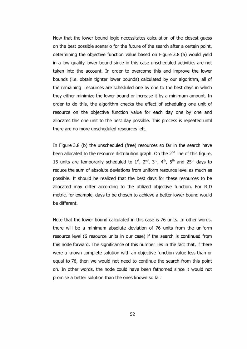
52

Now that the lower bound logic necessitates calculation of the closest guess

on the best possible scenario for the future of the search after a certain point,

determining the objective function value based on Figure 3.8 (a) would yield

in a low quality lower bound since in this case unscheduled activities are not

taken into the account. In order to overcome this and improve the lower

bounds (i.e. obtain tighter lower bounds) calculated by our algorithm, all of

the remaining resources are scheduled one by one to the best days in which

they either minimize the lower bound or increase it by a minimum amount. In

order to do this, the algorithm checks the effect of scheduling one unit of

resource on the objective function value for each day one by one and

allocates this one unit to the best day possible. This process is repeated until

there are no more unscheduled resources left.

In Figure 3.8 (b) the unscheduled (free) resources so far in the search have

been allocated to the resource distribution graph. On the 2nd line of this figure,

15 units are temporarily scheduled to 1st, 2nd, 3rd, 4th, 5th and 25th days to

reduce the sum of absolute deviations from uniform resource level as much as

possible. It should be realized that the best days for these resources to be

allocated may differ according to the utilized objective function. For RID

metric, for example, days to be chosen to achieve a better lower bound would

be different.

Note that the lower bound calculated in this case is 76 units. In other words,

there will be a minimum absolute deviation of 76 units from the uniform

resource level (6 resource units in our case) if the search is continued from

this node forward. The significance of this number lies in the fact that, if there

were a known complete solution with an objective function value less than or

equal to 76, then we would not need to continue the search from this point

on. In other words, the node could have been fathomed since it would not

promise a better solution than the ones known so far.

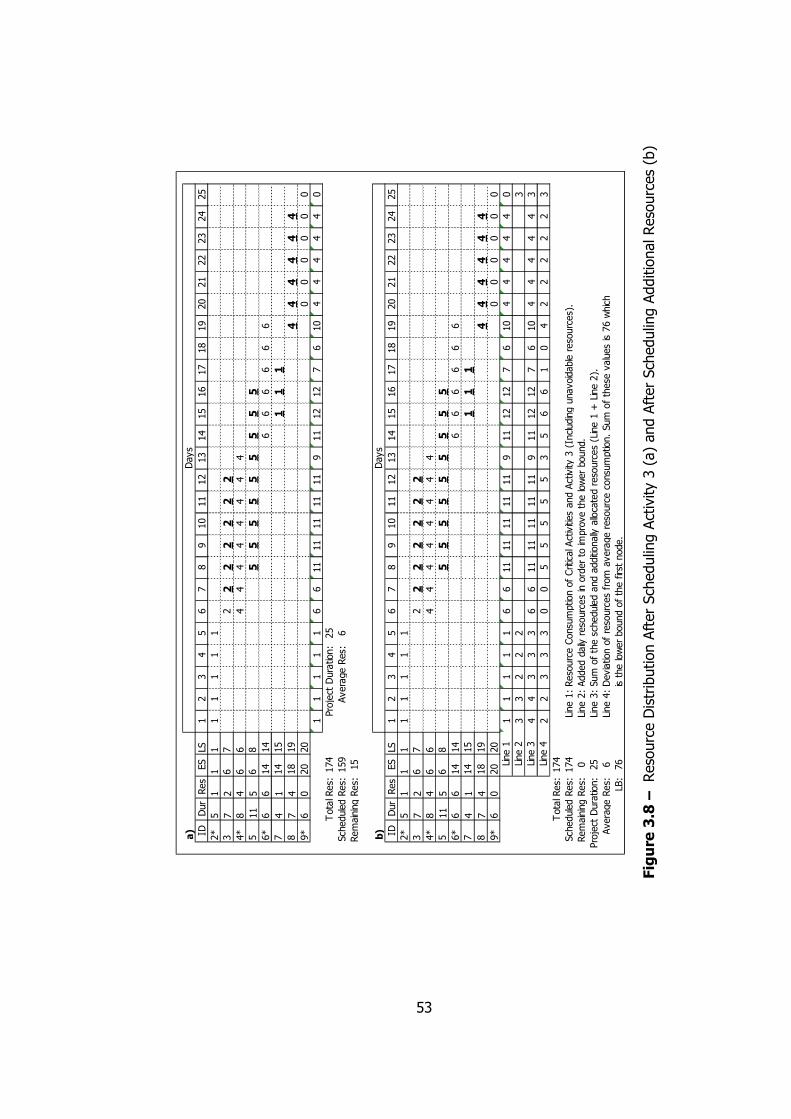
53

a) ID

DurRes

ES

LS1

23

45

67

89

10

11

12

13

14

15

16

17

18

19

20

21

22

23

24

25

2*

51

11

11

11

1

37

26

72

22

22

22

4*

84

66

44

44

44

44

511

56

85

55

55

55

55

6*

66

14

14

66

66

66

74

114

15

11

18

74

18

19

44

44

44

9*

60

20

20

00

00

00

11

11

16

611

11

11

11

11

911

12

12

76

10

44

44

40

Total Res:

174

Project Duration:

25

Scheduled Res:

159

Average Res:

6

Remaining Res:

15

b) ID

DurRes

ES

LS1

23

45

67

89

10

11

12

13

14

15

16

17

18

19

20

21

22

23

24

25

2*

51

11

11

11

1

37

26

72

22

22

22

4*

84

66

44

44

44

44

511

56

85

55

55

55

55

6*

66

14

14

66

66

66

74

114

15

11

18

74

18

19

44

44

44

9*

60

20

20

00

00

00

11

11

16

611

11

11

11

11

911

12

12

76

10

44

44

40

33

22

23

44

33

36

611

11

11

11

11

911

12

12

76

10

44

44

43

22

33

30

05

55

55

35

66

10

42

22

22

3

Total Res:

174

Scheduled Res:

174

Line 1:Resource Consumption of Critical Activities and Activity 3 (Including unavoidable resources).

Remaining Res:

0Line 2:Added daily resources in order to im

prove the lower bound.

Project Duration:

25

Line 3:Sum of the scheduled and additionally allocated resources (Line 1 + Line 2).

Average Res:

6Line 4:Deviation of resources from average resource consumption. Sum of these values is 76 which

LB:

76

is the lower bound of the first node.

Days

Line 1

Line 2

Line 4

Days

Line 3

Figure 3.8 – Resource Distribution After Scheduling Activity 3 (a) and After Scheduling Additional Resources (b)

54

Although allocation of free resources is an important improvement while

calculating the lower bounds for all objective functions in our study, it is

particularly important for RID metric. This is because application of this metric

requires the allocation of all resources to get an adequate estimate on the

overall idle times of resources. If there is a certain amount of unscheduled

resources, then it is not possible to estimate total idle days in the allocation

graph since there will be a possibility for the unscheduled resources to be

allocated to these idle durations and to reduce the lower bound calculated in

the following steps. For example RID value of the node can not be calculated

according to the resource distribution in Figure 3.8 (a). As seen on this figure,

RID value at this instant of the search is 9 units. Obviously, this value can not

be considered as a lower bound since there are 15 units of resources waiting

to be scheduled which may result in better lower bounds in the following

steps. It should be recalled that such a case can not be accepted since the

lower bound logic requires a guess on the best possible scenario regarding the

future search. Thus there should not be any possibility to obtain a partial or

complete solution after a node which is better than the lower bound

suggested in that node. This can be seen on the search tree in Figure 3.5,

which is obtained for MinDev objective function by employing the lower bound

improvement methods presented in Sections 3.4.2.1, 3.4.2.2 and 3.4.2.3. As

seen on this figure, lower bound of the node in which Activity 3 is scheduled

to start at the 6th day is 76 units as calculated in Figure 3.8 (b). It should also

be noted that in none of the nodes, calculated lower bound value is less than

the ones predicted by the parents of that node. In other words lower bound

values increase as the search tree is explored deeper. This situation also

reveals that the optimistic predictions (lower bounds) in nodes are not

realized (mostly) as the search proceeds. Therefore, lower bound values of

children nodes are lower than or, under best conditions, equal to the lower

bounds of their parents.

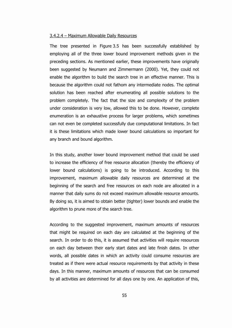
55

3.4.2.4 – Maximum Allowable Daily Resources

The tree presented in Figure 3.5 has been successfully established by

employing all of the three lower bound improvement methods given in the

preceding sections. As mentioned earlier, these improvements have originally

been suggested by Neumann and Zimmermann (2000). Yet, they could not

enable the algorithm to build the search tree in an effective manner. This is

because the algorithm could not fathom any intermediate nodes. The optimal

solution has been reached after enumerating all possible solutions to the

problem completely. The fact that the size and complexity of the problem

under consideration is very low, allowed this to be done. However, complete

enumeration is an exhaustive process for larger problems, which sometimes

can not even be completed successfully due computational limitations. In fact

it is these limitations which made lower bound calculations so important for

any branch and bound algorithm.

In this study, another lower bound improvement method that could be used

to increase the efficiency of free resource allocation (thereby the efficiency of

lower bound calculations) is going to be introduced. According to this

improvement, maximum allowable daily resources are determined at the

beginning of the search and free resources on each node are allocated in a

manner that daily sums do not exceed maximum allowable resource amounts.

By doing so, it is aimed to obtain better (tighter) lower bounds and enable the

algorithm to prune more of the search tree.

According to the suggested improvement, maximum amounts of resources

that might be required on each day are calculated at the beginning of the

search. In order to do this, it is assumed that activities will require resources

on each day between their early start dates and late finish dates. In other

words, all possible dates in which an activity could consume resources are

treated as if there were actual resource requirements by that activity in these

days. In this manner, maximum amounts of resources that can be consumed

by all activities are determined for all days one by one. An application of this,

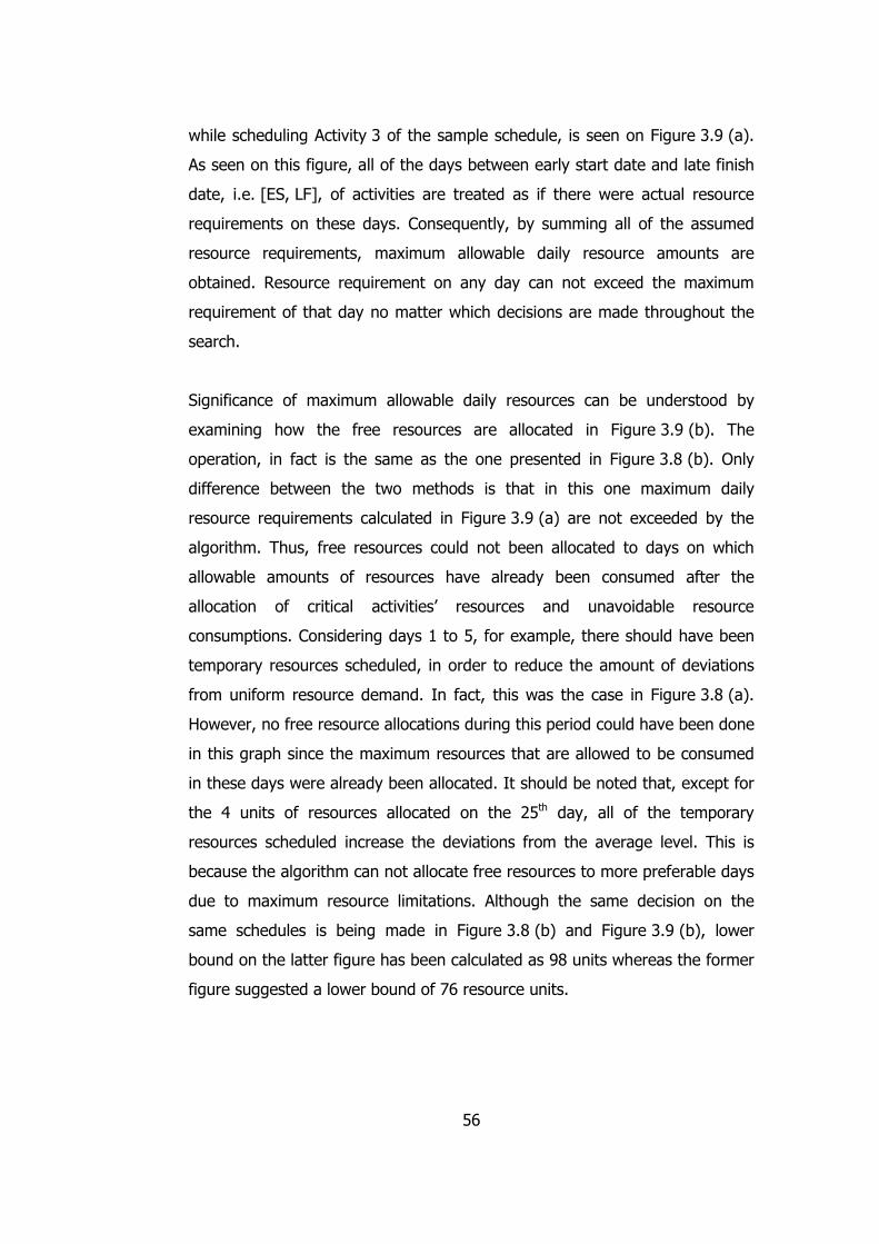
56

while scheduling Activity 3 of the sample schedule, is seen on Figure 3.9 (a).

As seen on this figure, all of the days between early start date and late finish

date, i.e. [ES, LF], of activities are treated as if there were actual resource

requirements on these days. Consequently, by summing all of the assumed

resource requirements, maximum allowable daily resource amounts are

obtained. Resource requirement on any day can not exceed the maximum

requirement of that day no matter which decisions are made throughout the

search.

Significance of maximum allowable daily resources can be understood by

examining how the free resources are allocated in Figure 3.9 (b). The

operation, in fact is the same as the one presented in Figure 3.8 (b). Only

difference between the two methods is that in this one maximum daily

resource requirements calculated in Figure 3.9 (a) are not exceeded by the

algorithm. Thus, free resources could not been allocated to days on which

allowable amounts of resources have already been consumed after the

allocation of critical activities’ resources and unavoidable resource

consumptions. Considering days 1 to 5, for example, there should have been

temporary resources scheduled, in order to reduce the amount of deviations

from uniform resource demand. In fact, this was the case in Figure 3.8 (a).

However, no free resource allocations during this period could have been done

in this graph since the maximum resources that are allowed to be consumed

in these days were already been allocated. It should be noted that, except for

the 4 units of resources allocated on the 25th day, all of the temporary

resources scheduled increase the deviations from the average level. This is

because the algorithm can not allocate free resources to more preferable days

due to maximum resource limitations. Although the same decision on the

same schedules is being made in Figure 3.8 (b) and Figure 3.9 (b), lower

bound on the latter figure has been calculated as 98 units whereas the former

figure suggested a lower bound of 76 resource units.

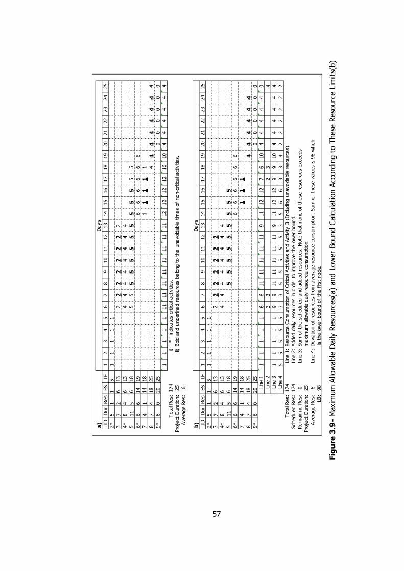
57

a) ID

DurRes

ES

LF1

23

45

67

89

10

11

12

13

14

15

16

17

18

19

20

21

22

23

24

25

2*

51

15

11

11

1

37

26

13

22

22

22

22

4*

84

613

44

44

44

44

511

56

18

55

55

55

55

55

55

5

6*

66

14

19

66

66

66

74

114

18

11

11

1

87

418

25

44

44

44

44

9*

60

20

25

00

00

00

11

11

111

11

11

11

11

11

11

11

12

12

12

12

16

10

44

44

44

Total Res:

174

i)" * " indicates critical activities.

Project Duration:

25

ii)Bold and underlined resources belong to the unavoidable times of non-critical activities.

Average Res:

6

b) ID

DurRes

ES

LF1

23

45

67

89

10

11

12

13

14

15

16

17

18

19

20

21

22

23

24

25

2*

51

15

11

11

1

37

26

13

22

22

22

24*

84

613

44

44

44

44

511

56

18

55

55

55

55

56*

66

14

19

66

66

66

74

114

18

11

18

74

18

25

44

44

44

9*

60

20

25

00

00

00

11

11

16

611

11

11

11

11

911

12

12

76

10

44

44

40

33

23

4

11

11

19

911

11

11

11

11

911

12

12

99

10

44

44

44

55

55

53

35

55

55

35

66

33

42

22

22

2

Total Res:

174

Line 1:Resource Consumption of Critical Activities and Activity 3 (Including unavoidable resources).

Scheduled Res:

174

Line 2:Added daily resources in order to improve the lower bound.

Remaining Res:

0Line 3:Sum of the scheduled and added resources. Note that none of these resources exceeds

Project Duration:

25

maximum allowable daily resource consumption.

Average Res:

6Line 4:Deviation of resources from average resource consumption. Sum of these values is 98 which

LB:

98

is the lower bound of the first node.

Days

Line 1

Days

Line 2

Line 3

Line 4

Figure 3.9- Maximum Allowable Daily Resources(a) and Lower Bound Calculation According to These Resource Limits(b)

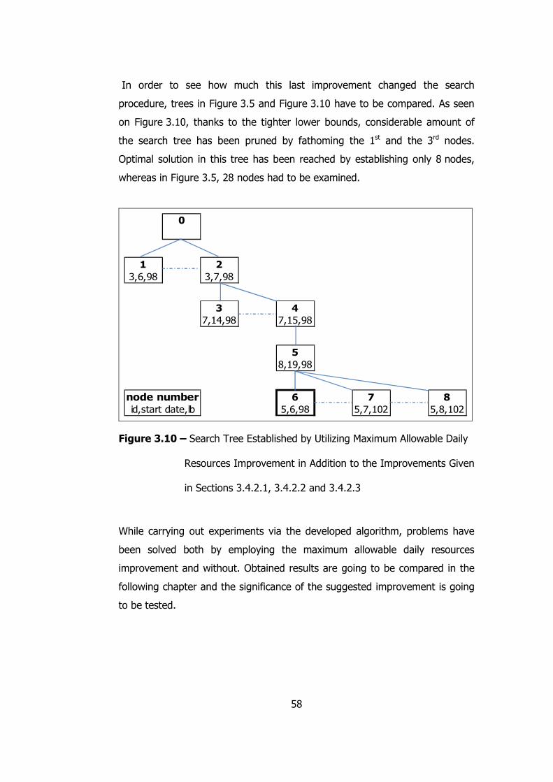
58

In order to see how much this last improvement changed the search

procedure, trees in Figure 3.5 and Figure 3.10 have to be compared. As seen

on Figure 3.10, thanks to the tighter lower bounds, considerable amount of

the search tree has been pruned by fathoming the 1st and the 3rd nodes.

Optimal solution in this tree has been reached by establishing only 8 nodes,

whereas in Figure 3.5, 28 nodes had to be examined.

0

1

3,6,98

2

3,7,98

3

7,14,98

4

7,15,98

5

8,19,98

6

5,6,98

7

5,7,102

8

5,8,102

node number id,start date,lb

Figure 3.10 – Search Tree Established by Utilizing Maximum Allowable Daily

Resources Improvement in Addition to the Improvements Given

in Sections 3.4.2.1, 3.4.2.2 and 3.4.2.3

While carrying out experiments via the developed algorithm, problems have

been solved both by employing the maximum allowable daily resources

improvement and without. Obtained results are going to be compared in the

following chapter and the significance of the suggested improvement is going

to be tested.

59

3.4.3 Choosing an Intermediate Node from Which to Branch Next

and Selecting the Activity to be Scheduled

In the beginning of Section 3.4 it has been indicated that the developed

branch and bound algorithm is based on a depth-first and least-lower-bound

criteria. According to the depth first rule, one of the nodes created in the

previous stage is chosen and the search is carried out downwards on the tree

node by node. If any branch is fathomed, i.e. none of the solutions that could

be obtained by further exploring that branch is promising, then the algorithm

retreats that branch upwards until a node which has not been totally explored

is encountered (Demeulemeester and Herroelen, 2002). Thus the algorithm

firstly explores the branches downwards until they are pruned or a leaf (a

complete solution) is reached, and then finds another node to be explored.

This procedure is repeated until all branches are explored or pruned. If

Figure 3.10 is considered once again, it can be observed that the depth-first

procedure explores a solution with an objective function value of 98 at the

very beginning of the search. After finding this solution, Node 1 and Node 3

are checked to see if they are to be explored any further or not. Since lower

bounds of these nodes were equal to the best known solution’s objective

function value so far, they were fathomed and the procedure has been

terminated.

During the exploration of a search tree, if there are two or more brother

nodes that might be explored further, then the one with the least (best) lower

bound is selected. This is simply because the node with the better lower

bound promises better solutions. In case there is a tie in this selection, then

the node which schedules the next activity to the latest start date is chosen.

After determining the node to be branched, another selection to be made is

about which activity to schedule in the next step. It has already been

mentioned that the activities’ total floats and feasible start times are being

calculated on each node considering the decisions made previously. Thus an

60

intermediate node which is to be branched further stores a valid list of

candidate activities with the updated total floats. From this list, activity with

the least amount of total float is chosen to be sequenced in the next step

where ties are broken by preferring the activity with the lower id number. By

employing this selection rule, branching in the upper levels of the search tree

is limited as much as possible to improve the computational efficiency.

3.4.4 Recognizing Non-promising Nodes and Optimal Solutions

Lower bounds calculated on each node enable the algorithm to differentiate

the promising nodes from the ones that need to be fathomed. At the

beginning of all searches, first complete solution reached is stored as the

current best solution. This solution, of course, is updated every time a better

solution is encountered by the algorithm. Throughout the search all of the

established nodes’ lower bound values are compared to the current best

solution’s lower bound value to ensure that non-promising nodes are

recognized and fathomed. Similarly each time a leaf (a complete schedule) is

encountered, its lower bound is checked against the objective function value

of the best complete solution so far. Leaves are recognized when the number

of scheduled activities in a node is equal to the total number of non critical

activities of the schedule under consideration. If a better solution than the

best solution known so far is detected at a leaf, this solution is assigned as the

current best. Current best solution at the end of the search procedure reveals

the optimal solution to the problem.

Throughout the search, feasibility of solutions needs not to be checked since

only valid start dates are considered while scheduling the activities. In other

words, the algorithm ensures feasibility by the manner through which it

constructs the solutions. Any partial or complete solutions include a set of

feasible start dates of the activities.

61

3.5 The Branch and Bound Procedure

In this section procedure followed by the introduced algorithm is going to be

explained step by step.

Step 1 – Initialization

1.1 Carry out forward and backward pass calculations. Determine

feasible start dates and total floats of activities according to the

early start schedule.

1.2 Determine the set of unscheduled activities (Initially equals to

the set of noncritical activities)

1.3 Initiate the resource utilization graph.

1.3.1 Allocate resources for critical activities.

1.3.2 Allocate resources required during unavoidable times of

non-critical activities.

Step 2 – Initial Depth-First Search

2.1 Select the activity with the least total float value from the list of

unscheduled activities. Break any tie by selecting the task with

the smallest id number.

2.2 Establish nodes by scheduling the selected activity to all its

feasible start dates (List of feasible start dates is obtained from

the early start schedule at the first level of the tree and from

the parent nodes at all other levels).

2.2.1 For each node established in the previous step, update

feasible start dates and total floats of activities

considering the decisions made so far.

2.2.2 Allocate resources of the scheduled activity. Do not

reschedule resources that are consumed in unavoidable

times of that activity since they have already been

allocated in Step 1.3.2.

62

2.2.3 Calculate lower bound value for each newly generated

node by applying “unscheduled resources improvement”

and “maximum allowable daily resources improvement”.

2.3 As long as there is at least one unscheduled activity, select the

node with the lowest (best) lower bound value. Break any tie

by selecting the node which schedules the activity to the latest

start date.

2.4 Repeat the procedure presented in steps 2.2 and 2.3 until there

are no more unscheduled activities (i.e. until first leaf nodes –

complete solutions are reached). Go to step 2.5 if all non-

critical activities are scheduled.

2.5 Determine the best complete solution (i.e. the complete

solution with the lowest objective function value) obtained.

Save the objective function value of this node as the current

best value and the corresponding solution (i.e. set of start

dates for the non-critical activities) as the current best solution.

Step 3 – Backtracking

3.1 Go one level up in the search tree and check for the nodes to

be explored (i.e. nodes that have no children yet and that have

a better lower bound value than the current best value.

3.1.1 If there is any unfathomed node without children and

with a lower bound value worse than the current best

value, then fathom this non-promising node. Delete lists

stored in this node to free the memory allocated to

these information. If there is no promising nodes in that

level go back to Step 3.1.

3.1.2 If there is any node without children and with a lower

bound value better than the current best value, then

discover this promising node further. If there are more

than one promising node with the same lower bound

63

value, select the node that schedules the activity to the

latest start date. For the next step; select the activity

with the least total float value stored in this node to

schedule. Break any ties by selecting activity with the

smallest id number.

3.1.3 Establish nodes by scheduling the selected activity in

the previous step to all its feasible start dates (List of

feasible start dates is obtained from the parent node).

3.1.3.1 For each node established in the previous step,

update feasible start dates and total floats of

activities considering the decisions made so far.

3.1.3.2 Allocate resources of the scheduled activity. Do

not reschedule resources that are consumed in

unavoidable times of that activity since they

have already been allocated in Step 1.3.2.

3.1.3.3 Calculate lower bound value for each newly

generated node by applying “unscheduled

resources improvement” and “maximum

allowable daily resources improvement”.

3.1.3.4 Fathom nodes that have lower bound values

equal to or more than the current best value.

3.1.4 As long as there is at least one unscheduled activity and

at least one promising node; select the node with the

lowest (best) lower bound value. Break any tie by

selecting the node which schedules the activity to the

latest start date. Repeat Steps 3.1.3 to 3.1.4. If a

complete solution is obtained go to Step 3.2.

3.1.5 In case there is no promising node among the newly

generated brother nodes go to Step 3.1.

3.2 Determine the best complete solution (i.e. the leaf node with

the lowest objective function value) obtained. Save the

objective function value of this node as the current best value

64

and the corresponding solution (i.e. set of start dates for the

non-critical activities) as the current best solution.

3.3 Go to Step 3.1 and repeat Steps 3.2 and 3.3 until all nodes in

the tree are either fathomed or further explored.

3.4 If all nodes in the tree are fathomed or explored, declare the

current best value as the optimal objective function value and

the corresponding solution as the optimal solution to the

problem. Then, terminate the program.

3.6 Coding the Algorithm

Branch and bound algorithm presented in this study has been coded in C++

computer language. Microsoft Visual Studio 2008 Professional Edition has

been used to compile codes.

For each node in the search tree, two structures have been introduced by the

algorithm. First of these structures stores information related to the position of

the node in the tree. The address of the parent node, addresses of the

brother nodes and addresses of the children nodes are stored in pointers of

this structure. Obviously, this information is required to enable the algorithm

to navigate through the list. Thus, even if a node is fathomed, this first

structure is not deleted to maintain the connections within the search tree.

The second structure, on the other hand, stores sets of partial or complete

solutions (i.e. lists of start dates for non-critical activities) and calculates lower

bounds associated with these solutions. Also, feasible start dates for the

unscheduled activities are stored and updated in the second structure. In

addition to these, it also tracks the list of unscheduled activities and

determines eligible activities that could be scheduled at any instant of search.

Since the data stored in the second structure is related only to the suggested

solution by that node, this structure is deleted as soon as that particular node

is fathomed. By doing this, the memory allocated to this structure is freed.

65

While coding the algorithm, pointers are commonly employed in order to save

time in storing and reading data, to establish branches within the search tree,

to remember the best solution encountered so far etc. Dynamic memory

allocation is employed to generate arrays of variable sizes. Also, vectors are

used to generate arrays of structures size of which are not known at the

beginning of the runtime.

As it has been explained in the previous section, the algorithm continuously

navigates through the tree to ensure optimality. While doing this, several

branches need to be retreated upwards to check whether there are any

promising nodes left undiscovered in the upper levels. Therefore, each time a

leaf node is encountered and each time all brother nodes at a specific level

are fathomed, a function that directs the search to the upper levels is called

by the algorithm. In fact, it is these recursive function calls that limit the size

of the problem that could be solved effectively by the algorithm. In order to

enable the algorithm to do more recursive function calls, stack reserve size,

which specifies the total stack allocation size in virtual memory of the

compiler, was increased to 20 MB during the experimentations.

66

CHAPTER 4

VALIDATION AND COMPUTATIONAL RESULTS

In this chapter, validation of the developed algorithm is explained and

computational experiments are presented. Also, significance of the maximum

allowable daily resource improvement suggested to calculate tighter lower

bounds is tested.

4.1 Validating the Algorithm

In order to ensure that the algorithm is capable of successfully exploring the

search space and locating the global optima, preliminary experimentations

have been conducted. Some of the few known solutions of RLP available in

literature have been used in these experiments and results obtained via our

algorithm were compared to the solutions from previous studies. In addition

to this, some other problems have been solved to optimality via linear-integer

programming and results obtained from these analyses were compared to the

ones of the suggested branch and bound procedure.

As mentioned previously, El-Rayes and Jun (2009) reported solutions obtained

by their metaheuristic based method for the RLP. In this study, a single

resource network which included 6 critical and 14 non critical activities has

been addressed. Results obtained by the developed GA optimization module

for traditional objective functions, such as SSQR, MinDev and Minimum

Moment in addition to the new metrics suggested by the researchers, which

are Release and Rehire and RID, have been reported.

67

Same application example has been solved by our branch and bound

algorithm utilizing the SSQR, MinDev, RID and RID+MRD metrics. In all of

these experiments, feasible solutions with the same objective function values

suggested by El-Rayes and Jun (2009) have been found successfully. This, in

fact, also revealed that the results obtained by the GA module of the

researchers were the global optimal solutions.

A similar validation process has been followed while addressing example

problems presented by Son and Skibniewski (1999). These two example

networks consisted of 13 and 15 activities (including dummy start and dummy

finish activities) respectively and were solved by the suggested multiheuristic

approach to minimize SSQR value implied by the resource distribution graphs.

Branch and bound algorithm developed in our study successfully solved these

single-resource networks and obtained the same objective function values

presented in the original paper. Again, this situation indicates that the results

obtained by Son and Skibniewski (1999) were the global optimum solutions

for the problems.

The last problem from the literature used for validation purposes was the

small size network of Easa (1989). Minimum absolute deviation possible for

this single resource network which consists of 7 activities has been

determined employing integer-linear optimization and results are compared to

the solution of our branch and bound algorithm.

Within the context of our study, some networks other than the ones presented

in the preceding paragraphs have also been solved to optimality via the linear

programming software, AIMMS 3.10. This is done to compare the results of

the branch and bound algorithm to the ones obtained by the linear

programming procedure. 6 single resource networks which consisted of 13 to

20 activities have been solved by the two methods and optimum MinDev

schedules have been determined successfully both by the branch and bound

algorithm and the linear programming method. Unfortunately, this type of

68

validation could be done for MinDev metric only, since other three objective

functions could not been utilized in linear programming. Also the fact that the

time and effort required to input variables and constraints to the linear

programming software were considerably high, limited the number of

schedules solved via this method.

Throughout the validation process, 1 solution for RID metric, 1 solution for

RID+MRD metric, 3 solutions for SSQR metric and 8 solutions for MinDev

metric have been verified either by comparing our results to exact solutions or

to the best known solutions in the literature. Moreover, some search trees

established by the algorithm for small size multiple resource schedules have

been checked node by node in order to ensure that the activity selections,

total float updates and lower bound calculations are being done correctly.

Details of all abovementioned solutions are going to be presented in the next

section together with other computational experiment results.

4.2 Computational Results

The branch and bound algorithm, coding details of which are presented in

Section 3.6, has been developed in C++ programming language. All

experimentations have been carried out on a PC with 2 GB RAM and an Intel

Core 2 Duo 3.00 GHz Processing Unit. The computer was run by Windows 7

Professional (32 bit) operating system.

As in most branch and bound based studies, main performance measure of

this study is the CPU time spent by the algorithm while solving problems. This

quantity was obtained by measuring the time spent while instructions are

being executed. By definition, input and output durations are not included in

the CPU time. In addition to this measure, number of nodes established by the

algorithm in order to locate the optimal solutions are presented both for

comparison reasons and to give an indication of the size of the search tree

under consideration.

69

20 resource leveling problems have been solved for experimentation

purposes. All of the objective functions presented in Chapter 3.1, i.e. SSQR,

MinDev, RID and RID+MRD metrics, have been utilized for these problems.

Resource distribution graphs of both single resource and multiple resource (4

resource types) modes of the problems have been leveled. Two different

types of algorithms are employed to solve single resource problems. One of

these did include all of the improvements presented in Sections 3.4.2.1 to

3.4.2.4. The other one, on the other hand, did not incorporate the last lower

bound improvement suggested in this study, i.e. the maximum allowable daily

resource limitation. In this manner, results obtained by the two types of

algorithms have been compared in order to find out whether the suggested

improvement made any significant contribution to the performance or not. All

computational results obtained from the experiments are presented in

Tables 4.1 to 4.10.

Some of the problems used for experimentation and validation purposes were

available in literature in single resource modes. Networks and resource rates

of these problems have directly been used. To derive a multi resource

problem, however, remaining three types of resources are generated

randomly for each activity. Problems 1, 12, 15, 16 and 18, presented in the

following tables are problems of this type. Activity numbers of these problems

range from 12 to 22.

In addition to the RLPs, several networks which did not include any resource

considerations were also available in literature. These networks have been

transformed to leveling problems by randomly generating daily resource

requirements for each task. Problems 2, 4, 5, 6, 8, 13, 14, 17 and 19 given in

the following tables are obtained in this manner. Activity numbers of these

problems ranged from 10 to 21.

6 of the 20 problems used for experimentation purposes have been generated

while developing the branch and bound procedure. These problems originally

70

intend to test certain capabilities of the algorithm such as solving RLPs with

multiple critical paths etc. The networks and resource requirements of these

problems are generated by hand. Therefore, they may tend to be biased.

Thus, the number of such networks is kept limited. Problems 3, 7, 9, 10, 11

and 12 are obtained in this manner. These problems include 8 to 20 activities.

Due to the characteristics of the developed algorithm, networks need to start

and finish with dummy activities. Therefore dummy start and dummy finish

activities with zero duration and zero resource requirements are included to

the problems whenever necessary. While generating the resource

requirements of activities, random number generator of Microsoft Excel has

been employed. A resource leveling problem set with unbiased, small size

problems was aimed to be obtained. Information on the precedence relations

and resource requirements of activities for all problems is given in Appendix A.

In the following tables, CPU times required to solve the problems and number

of nodes established by the algorithm to ensure optimality are given for all

objective functions defined in Section 3.1. Results for all metrics are reviewed

in 3 columns. First columns belong to the problems which require 4 resource

types, whereas second and third columns represent results obtained for single

resource modes of the same networks. Results given in the second columns

differ from the ones in the third column in that all lower bound improvements

have been utilized in these experiments. Third columns, however, tabulate the

performance of the algorithm without limiting the daily resource requirements.

Optimal objective function values obtained at the end of our analyses are also

given in the provided tables. These values are calculated as explained in

Section 3.1. While calculating the optimal objective function values for multi

resource projects, weights of each resource are assumed to be equal and are

normalized to 1. In other words, “wi” values of each resource type are taken

as 0.25 since there were 4 types of resources included in the multiple

resource networks.

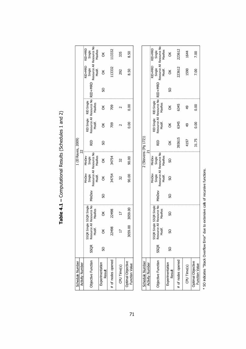
71

Schedule Number

Activity Number

Objective Function

SSQR

SSQR Single

Resource All

Modif.

SSQR Single

Resource No

MaxRes

MinDev

MinDev

Single

Resource All

Modif.

MinDev

Single

Resource No

MaxRes

RID

RID Single

Resource All

Modif.

RID Single

Resource No

MaxRes

RID+MRD

RID+MRD

Single

Resource All

Modif.

RID+MRD

Single

Resource No

MaxRes

Experim

entation

Result

SO

OK

OK

SO

OK

OK

SO

OK

OK

SO

OK

OK

# of nodes opened

22498

22498

34754

34754

709

709

113332

113332

CPU Time(s)

17

17

32

32

22

292

335

Optim

al O

bjective

Function Value

3059.00

3059.00

90.00

90.00

0.00

0.00

8.50

8.50

Schedule Number

Activity Number

Objective Function

SSQR

SSQR Single

Resource All

Modif.

SSQR Single

Resource No

MaxRes

MinDev

MinDev

Single

Resource All

Modif.

MinDev

Single

Resource No

MaxRes

RID

RID Single

Resource All

Modif.

RID Single

Resource No

MaxRes

RID+MRD

RID+MRD

Single

Resource All

Modif.

RID+MRD

Single

Resource No

MaxRes

Experim

entation

Result

SO

SO

SO

SO

SO

SO

OK

OK

OK

SO

OK

OK

# of nodes opened

393615

6345

6345

223612

223612

CPU Time(s)

4197

49

49

1590

1644

Optim

al O

bjective

Function Value

31.75

0.00

0.00

7.00

7.00

* SO indicates "Stack Overflow Error" due to extensive calls of recursive functions.

1 (El Rayes, 2009)

2 (Stevens (Pg 172))

22

21

Table 4.1 – Computational Results (Schedules 1 and 2)

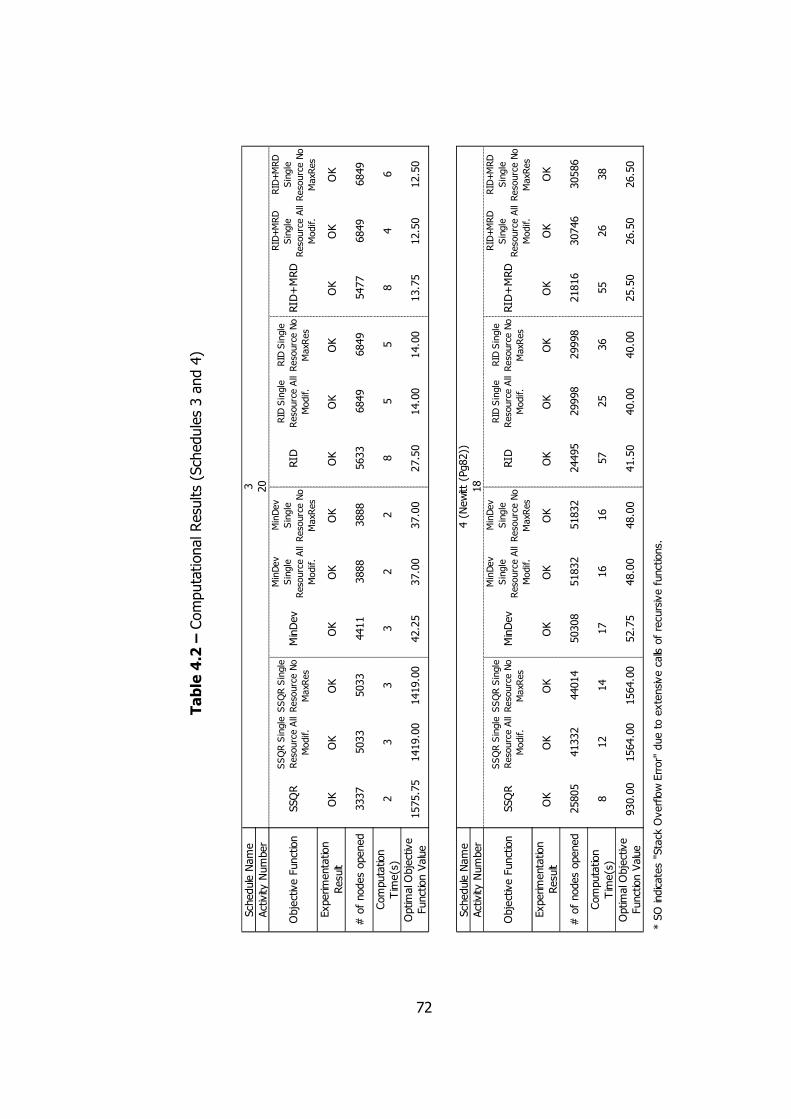
72

Schedule Name

Activity Number

Objective Function

SSQR

SSQR Single

Resource All

Modif.

SSQR Single

Resource No

MaxRes

MinDev

MinDev

Single

Resource All

Modif.

MinDev

Single

Resource No

MaxRes

RID

RID Single

Resource All

Modif.

RID Single

Resource No

MaxRes

RID+MRD

RID+MRD

Single

Resource All

Modif.

RID+MRD

Single

Resource No

MaxRes

Experim

entation

Result

OK

OK

OK

OK

OK

OK

OK

OK

OK

OK

OK

OK

# of nodes opened

3337

5033

5033

4411

3888

3888

5633

6849

6849

5477

6849

6849

Computation

Time(s)

23

33

22

85

58

46

Optim

al O

bjective

Function Value

1575.75

1419.00

1419.00

42.25

37.00

37.00

27.50

14.00

14.00

13.75

12.50

12.50

Schedule Name

Activity Number

Objective Function

SSQR

SSQR Single

Resource All

Modif.

SSQR Single

Resource No

MaxRes

MinDev

MinDev

Single

Resource All

Modif.

MinDev

Single

Resource No

MaxRes

RID

RID Single

Resource All

Modif.

RID Single

Resource No

MaxRes

RID+MRD

RID+MRD

Single

Resource All

Modif.

RID+MRD

Single

Resource No

MaxRes

Experim

entation

Result

OK

OK

OK

OK

OK

OK

OK

OK

OK

OK

OK

OK

# of nodes opened

25805

41332

44014

50308

51832

51832

24495

29998

29998

21816

30746

30586

Computation

Time(s)

812

14

17

16

16

57

25

36

55

26

38

Optim

al O

bjective

Function Value

930.00

1564.00

1564.00

52.75

48.00

48.00

41.50

40.00

40.00

25.50

26.50

26.50


3

4 (Newitt (Pg82))

20

18


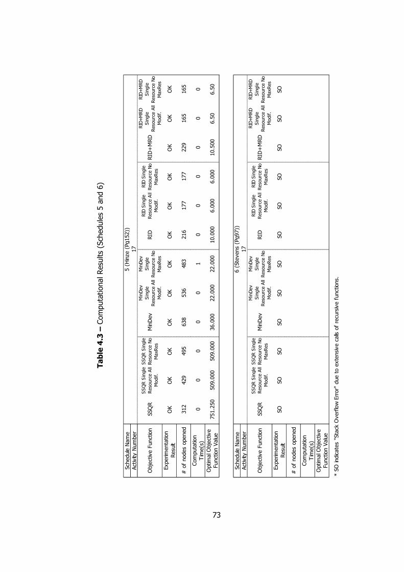
73

Schedule Name

Activity Number

Objective Function

SSQR

SSQR Single

Resource All

Modif.

SSQR Single

Resource No

MaxRes

MinDev

MinDev

Single

Resource All

Modif.

MinDev

Single

Resource No

MaxRes

RID

RID Single

Resource All

Modif.

RID Single

Resource No

MaxRes

RID+MRD

RID+MRD

Single

Resource All

Modif.

RID+MRD

Single

Resource No

MaxRes

Experim

entation

Result

OK

OK

OK

OK

OK

OK

OK

OK

OK

OK

OK

OK

# of nodes opened

312

429

495

638

536

483

216

177

177

229

165

165

Computation

Time(s)

00

00

01

00

00

00

Optim

al O

bjective

Function Value

751.250

509.000

509.000

36.000

22.000

22.000

10.000

6.000

6.000

10.500

6.50

6.50

Schedule Name

Activity Number

Objective Function

SSQR

SSQR Single

Resource All

Modif.

SSQR Single

Resource No

MaxRes

MinDev

MinDev

Single

Resource All

Modif.

MinDev

Single

Resource No

MaxRes

RID

RID Single

Resource All

Modif.

RID Single

Resource No

MaxRes

RID+MRD

RID+MRD

Single

Resource All

Modif.

RID+MRD

Single

Resource No

MaxRes

Experim

entation

Result

SO

SO

SO

SO

SO

SO

SO

SO

SO

SO

SO

SO

# of nodes opened

Computation

Time(s)

Optim

al O

bjective

Function Value


5 (Hinze (Pg152))

6 (Stevens (Pg97))

17

17


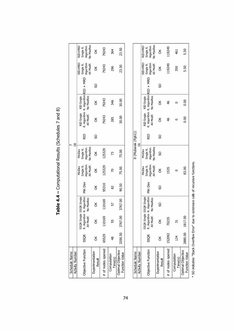
74

Schedule Name

Activity Number

Objective Function

SSQR

SSQR Single

R. Algorithm

All Modif.

SSQR Single

R. Algorithm

No MaxRes

Min Dev

MinDev

Single R.

Algorithm

All Modif.

MinDev

Single R.

Algorithm

No MaxRes

RID

RID Single

R. Algorithm

All Modif.

RID Single

R. Algorithm

No MaxRes

RID + M

RD

RID+MRD

Single R.

Algorithm

All Modif.

RID+MRD

Single R.

Algorithm

No MaxRes

Experim

entation

Result

OK

OK

OK

OK

OK

OK

SO

OK

OK

SO

OK

OK

# of nodes opened

65529

110169

110169

95310

125329

125329

79243

79243

79243

79243

Computation

Time(s)

48

55

57

82

70

73

285

346

296

364

Optim

al O

bjective

Function Value

3200.50

3767.00

3767.00

90.50

75.00

75.00

30.00

30.00

23.50

23.50

Schedule Name

Activity Number

Objective Function

SSQR

SSQR Single

R. Algorithm

All Modif.

SSQR Single

R. Algorithm

No MaxRes

Min Dev

MinDev

Single R.

Algorithm

All Modif.

MinDev

Single R.

Algorithm

No MaxRes

RID

RID Single

R. Algorithm

All Modif.

RID Single

R. Algorithm

No MaxRes

RID + M

RD

RID+MRD

Single R.

Algorithm

All Modif.

RID+MRD

Single R.

Algorithm

No MaxRes

Experim

entation

Result

OK

OK

SO

SO

OK

SO

SO

OK

OK

SO

OK

OK

# of nodes opened

152092

70235

1535

46

46

119249

119249

Computation

Time(s)

124

31

00

0350

461

Optim

al O

bjective

Function Value

2880.00

1817.00

83.00

0.00

0.00

5.50

5.50


167 18

8 (Mubarak (Pg61))


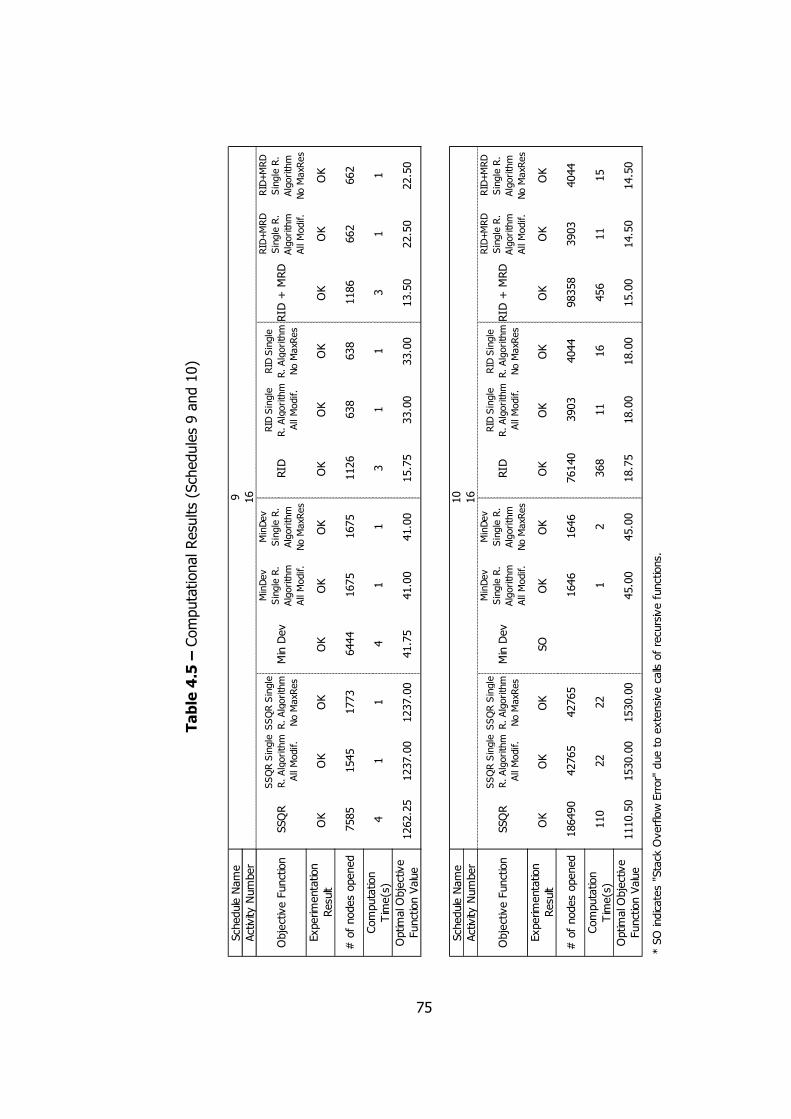
75

Schedule Name

Activity Number

Objective Function

SSQR

SSQR Single

R. Algorithm

All Modif.

SSQR Single

R. Algorithm

No MaxRes

Min Dev

MinDev

Single R.

Algorithm

All Modif.

MinDev

Single R.

Algorithm

No MaxRes

RID

RID Single

R. Algorithm

All Modif.

RID Single

R. Algorithm

No MaxRes

RID + M

RD

RID+MRD

Single R.

Algorithm

All Modif.

RID+MRD

Single R.

Algorithm

No MaxRes

Experim

entation

Result

OK

OK

OK

OK

OK

OK

OK

OK

OK

OK

OK

OK

# of nodes opened

7585

1545

1773

6444

1675

1675

1126

638

638

1186

662

662

Computation

Time(s)

41

14

11

31

13

11

Optim

al O

bjective

Function Value

1262.25

1237.00

1237.00

41.75

41.00

41.00

15.75

33.00

33.00

13.50

22.50

22.50

Schedule Name

Activity Number

Objective Function

SSQR

SSQR Single

R. Algorithm

All Modif.

SSQR Single

R. Algorithm

No MaxRes

Min Dev

MinDev

Single R.

Algorithm

All Modif.

MinDev

Single R.

Algorithm

No MaxRes

RID

RID Single

R. Algorithm

All Modif.

RID Single

R. Algorithm

No MaxRes

RID + M

RD

RID+MRD

Single R.

Algorithm

All Modif.

RID+MRD

Single R.

Algorithm

No MaxRes

Experim

entation

Result

OK

OK

OK

SO

OK

OK

OK

OK

OK

OK

OK

OK

# of nodes opened

186490

42765

42765

1646

1646

76140

3903

4044

98358

3903

4044

Computation

Time(s)

110

22

22

12

368

11

16

456

11

15

Optim

al O

bjective

Function Value

1110.50

1530.00

1530.00

45.00

45.00

18.75

18.00

18.00

15.00

14.50

14.50


16

10

169


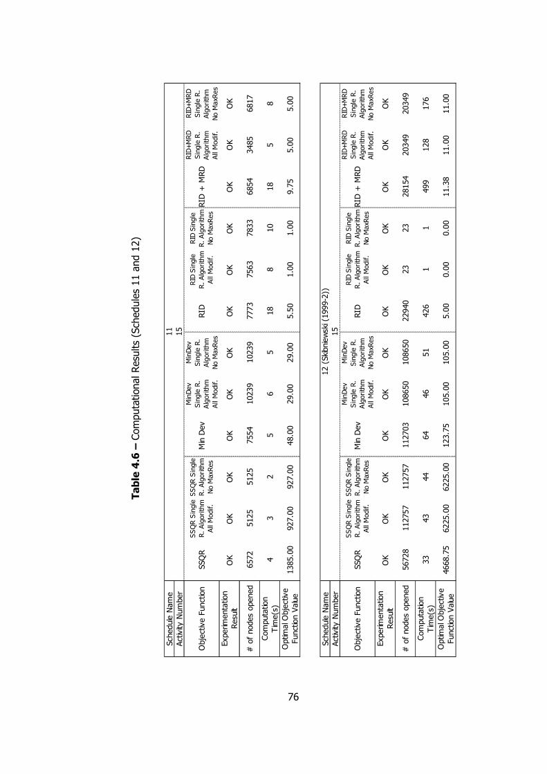
76

Schedule Name

Activity Number

Objective Function

SSQR

SSQR Single

R. Algorithm

All Modif.

SSQR Single

R. Algorithm

No MaxRes

Min Dev

MinDev

Single R.

Algorithm

All Modif.

MinDev

Single R.

Algorithm

No MaxRes

RID

RID Single

R. Algorithm

All Modif.

RID Single

R. Algorithm

No MaxRes

RID + M

RD

RID+MRD

Single R.

Algorithm

All Modif.

RID+MRD

Single R.

Algorithm

No MaxRes

Experim

entation

Result

OK

OK

OK

OK

OK

OK

OK

OK

OK

OK

OK

OK

# of nodes opened

6572

5125

5125

7554

10239

10239

7773

7563

7833

6854

3485

6817

Computation

Time(s)

43

25

65

18

810

18

58

Optim

al Objective

Function Value

1385.00

927.00

927.00

48.00

29.00

29.00

5.50

1.00

1.00

9.75

5.00

5.00

Schedule Name

Activity Number

Objective Function

SSQR

SSQR Single

R. Algorithm

All Modif.

SSQR Single

R. Algorithm

No MaxRes

Min Dev

MinDev

Single R.

Algorithm

All Modif.

MinDev

Single R.

Algorithm

No MaxRes

RID

RID Single

R. Algorithm

All Modif.

RID Single

R. Algorithm

No MaxRes

RID + M

RD

RID+MRD

Single R.

Algorithm

All Modif.

RID+MRD

Single R.

Algorithm

No MaxRes

Experim

entation

Result

OK

OK

OK

OK

OK

OK

OK

OK

OK

OK

OK

OK

# of nodes opened

56728

112757

112757

112703

108650

108650

22940

23

23

28154

20349

20349

Computation

Time(s)

33

43

44

64

46

51

426

11

499

128

176

Optim

al Objective

Function Value

4668.75

6225.00

6225.00

123.75

105.00

105.00

5.00

0.00

0.00

11.38

11.00

11.00

11

12 (Skibniewski (1999-2))

15

15


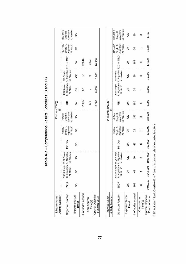
77

Schedule Name

Activity Number

Objective Function

SSQR

SSQR Single

R. Algorithm

All Modif.

SSQR Single

R. Algorithm

No MaxRes

Min Dev

MinDev

Single R.

Algorithm

All Modif.

MinDev

Single R.

Algorithm

No MaxRes

RID

RID Single

R. Algorithm

All Modif.

RID Single

R. Algorithm

No MaxRes

RID + M

RD

RID+MRD

Single R.

Algorithm

All Modif.

RID+MRD

Single R.

Algorithm

No MaxRes

Experim

entation

Result

SO

SO

SO

SO

SO

SO

OK

OK

OK

OK

SO

SO

# of nodes opened

23082

67

67

389286

Computation

Time(s)

139

00

1803

Optim

al Objective

Function Value

0.000

0.000

0.000

16.500

Schedule Name

Activity Number

Objective Function

SSQR

SSQR Single

R. Algorithm

All Modif.

SSQR Single

R. Algorithm

No MaxRes

Min Dev

MinDev

Single R.

Algorithm

All Modif.

MinDev

Single R.

Algorithm

No MaxRes

RID

RID Single

R. Algorithm

All Modif.

RID Single

R. Algorithm

No MaxRes

RID + M

RD

RID+MRD

Single R.

Algorithm

All Modif.

RID+MRD

Single R.

Algorithm

No MaxRes

Experim

entation

Result

OK

OK

OK

OK

OK

OK

OK

OK

OK

OK

OK

OK

# of nodes opened

105

45

60

45

22

195

180

30

30

165

30

30

Computation

Time(s)

01

00

00

00

00

00

Optim

al Objective

Function Value

1406.250

1043.000

1043.000

102.000

138.000

138.000

6.000

10.000

10.000

17.500

11.50

11.50


13 (Leu (2000))

14 (Newitt (Pg121))

15

14


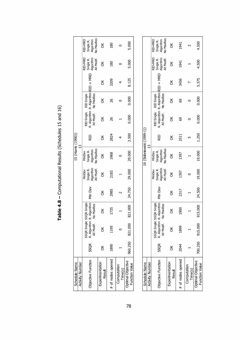
78

Schedule Name

Activity Number

Objective Function

SSQR

SSQR Single

R. Algorithm

All Modif.

SSQR Single

R. Algorithm

No MaxRes

Min Dev

MinDev

Single R.

Algorithm

All Modif.

MinDev

Single R.

Algorithm

No MaxRes

RID

RID Single

R. Algorithm

All Modif.

RID Single

R. Algorithm

No MaxRes

RID + M

RD

RID+MRD

Single R.

Algorithm

All Modif.

RID+MRD

Single R.

Algorithm

No MaxRes

Experim

entation

Result

OK

OK

OK

OK

OK

OK

OK

OK

OK

OK

OK

OK

# of nodes opened

1890

1195

1735

2985

2183

1968

2824

26

26

3209

180

180

Computation

Time(s)

10

12

10

41

04

00

Optim

al O

bjective

Function Value

960.250

821.000

821.000

34.750

29.000

29.000

3.500

0.000

0.000

8.125

5.000

5.000

Schedule Name

Activity Number

Objective Function

SSQR

SSQR Single

R. Algorithm

All Modif.

SSQR Single

R. Algorithm

No MaxRes

Min Dev

MinDev

Single R.

Algorithm

All Modif.

MinDev

Single R.

Algorithm

No MaxRes

RID

RID Single

R. Algorithm

All Modif.

RID Single

R. Algorithm

No MaxRes

RID + M

RD

RID+MRD

Single R.

Algorithm

All Modif.

RID+MRD

Single R.

Algorithm

No MaxRes

Experim

entation

Result

OK

OK

OK

OK

OK

OK

OK

OK

OK

OK

OK

OK

# of nodes opened

2044

1899

1900

2317

1397

1397

2511

69

69

3436

1941

1941

Computation

Time(s)

11

11

01

50

07

12

Optim

al O

bjective

Function Value

700.250

915.000

915.000

24.500

19.000

19.000

1.250

0.000

0.000

5.375

4.500

4.500

15 (Harris (1990))

16 (Skibniewski (1999-1))

13

13


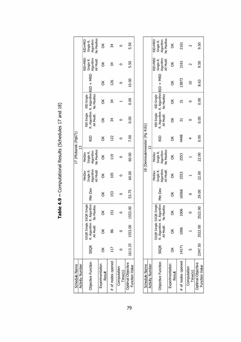
79

Schedule Name

Activity Number

Objective Function

SSQR

SSQR Single

R. Algorithm

All Modif.

SSQR Single

R. Algorithm

No MaxRes

Min Dev

MinDev

Single R.

Algorithm

All Modif.

MinDev

Single R.

Algorithm

No MaxRes

RID

RID Single

R. Algorithm

All Modif.

RID Single

R. Algorithm

No MaxRes

RID + M

RD

RID+MRD

Single R.

Algorithm

All Modif.

RID+MRD

Single R.

Algorithm

No MaxRes

Experim

entation

Result

OK

OK

OK

OK

OK

OK

OK

OK

OK

OK

OK

OK

# of nodes opened

117

86

151

153

105

119

122

34

34

126

34

34

Computation

Time(s)

00

00

00

00

10

00

Optim

al O

bjective

Function Value

1613.25

1553.00

1553.00

53.75

60.00

60.00

7.00

0.00

0.00

10.00

5.50

5.50

Schedule Name

Activity Number

Objective Function

SSQR

SSQR Single

R. Algorithm

All Modif.

SSQR Single

R. Algorithm

No MaxRes

Min Dev

MinDev

Single R.

Algorithm

All Modif.

MinDev

Single R.

Algorithm

No MaxRes

RID

RID Single

R. Algorithm

All Modif.

RID Single

R. Algorithm

No MaxRes

RID + M

RD

RID+MRD

Single R.

Algorithm

All Modif.

RID+MRD

Single R.

Algorithm

No MaxRes

Experim

entation

Result

OK

OK

OK

OK

OK

OK

OK

OK

OK

OK

OK

OK

# of nodes opened

14171

1006

1006

16566

2553

2553

4448

31

31

13873

2161

2161

Computation

Time(s)

51

06

11

40

010

22

Optim

al O

bjective

Function Value

2347.50

3522.00

3522.00

29.00

22.00

22.00

0.00

0.00

0.00

8.63

9.50

9.50

17 (Mubarak (Pg67))

18 (Demeulemeester (Pg 416))

13

12


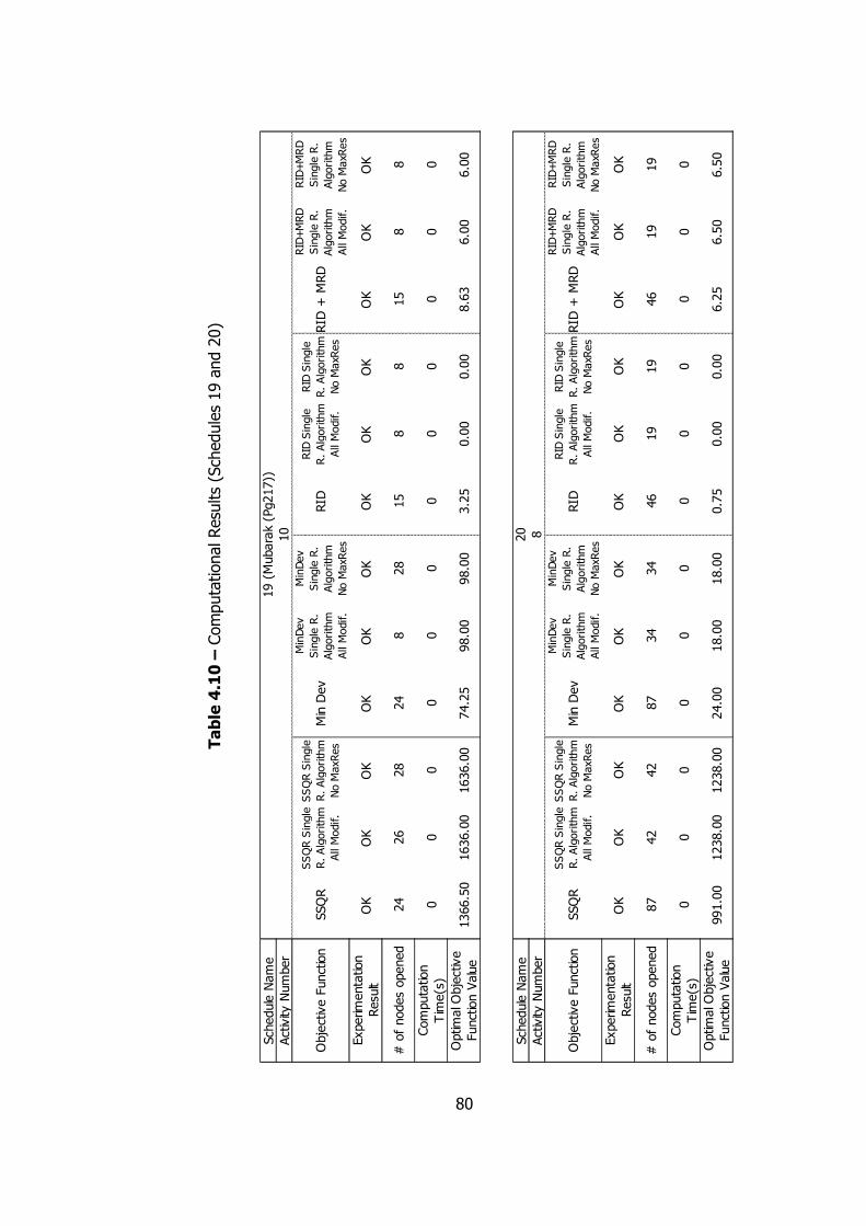
80

Schedule Name

Activity Number

Objective Function

SSQR

SSQR Single

R. Algorithm

All Modif.

SSQR Single

R. Algorithm

No MaxRes

Min Dev

MinDev

Single R.

Algorithm

All Modif.

MinDev

Single R.

Algorithm

No MaxRes

RID

RID Single

R. Algorithm

All Modif.

RID Single

R. Algorithm

No MaxRes

RID + M

RD

RID+MRD

Single R.

Algorithm

All Modif.

RID+MRD

Single R.

Algorithm

No MaxRes

Experim

entation

Result

OK

OK

OK

OK

OK

OK

OK

OK

OK

OK

OK

OK

# of nodes opened

24

26

28

24

828

15

88

15

88

Computation

Time(s)

00

00

00

00

00

00

Optim

al O

bjective

Function Value

1366.50

1636.00

1636.00

74.25

98.00

98.00

3.25

0.00

0.00

8.63

6.00

6.00

Schedule Name

Activity Number

Objective Function

SSQR

SSQR Single

R. Algorithm

All Modif.

SSQR Single

R. Algorithm

No MaxRes

Min Dev

MinDev

Single R.

Algorithm

All Modif.

MinDev

Single R.

Algorithm

No MaxRes

RID

RID Single

R. Algorithm

All Modif.

RID Single

R. Algorithm

No MaxRes

RID + M

RD

RID+MRD

Single R.

Algorithm

All Modif.

RID+MRD

Single R.

Algorithm

No MaxRes

Experim

entation

Result

OK

OK

OK

OK

OK

OK

OK

OK

OK

OK

OK

OK

# of nodes opened

87

42

42

87

34

34

46

19

19

46

19

19

Computation

Time(s)

00

00

00

00

00

00

Optim

al O

bjective

Function Value

991.00

1238.00

1238.00

24.00

18.00

18.00

0.75

0.00

0.00

6.25

6.50

6.50

19 (Mubarak (Pg217))

20

10 8


81

One of the most evident indications of network complexity is the number of

activities included in a schedule. Therefore, problems in the above tables are

sorted according to the decreasing activity numbers. If the results are

examined, it can be realized that some problems in Tables 4.1 to 4.7, i.e. with

higher numbers of activities, could not be solved successfully by the algorithm

for some objective functions. This situation is reported with the letters “SO”,

which stands for the stack overflow error. This type of error, which is caused

by too much memory usage due extensive calls to recursive functions,

prevented the solution of 19 multi resource and 9 single resource problems

out of 80 instances. In fact, it is stack overflow error that constituted the most

significant barrier for the algorithm for not being able to solve medium and

large size problems. Probable ways to overcome stack overflow error are

going to be suggested later as a further study option. At this point, however,

it should be indicated that the main reason for this problem to occur is the low

random access memory (RAM) capacity of the computer on which

experimentations have been carried out.

Although some instances could not be solved due to the stack overflow error,

branch and bound algorithm was still able to solve most of the multi resource

and single resource instances. For SSQR objective function, 16 multiple and 16

single resource problems out of 20 instances have been solved successfully,

whereas for MinDev metric these values turned out to be 14 for multiple

resource and 16 for single resource networks. As to the other objective

functions, 16 multiple resource and 19 single resource instances for RID

metric and 15 multiple resource and 18 single resource instances for

RID+MRD metric could be solved to optimality. Considering the results

reported in Tables 4.6 to 4.10, it can be commented that the developed

procedure can effectively deal with problems including up to 15 activities. For

problems with 15 to 22 activities, however, the algorithm might fail in finding

a solution due to stack overflow error.

82

As mentioned in previous chapters, one of the most significant drawbacks of

exact methods is that they require higher computation time compared to

heuristic based methods. To check whether a developed algorithm is suitable

for practical purposes, it is a commonly employed method to measure the

amount of problems that can be solved within a reasonable amount of time.

Introduced procedure in this study has been experimented with 20 RLPs in a

PC with the characteristics given at the beginning of this section and it has

been observed that all of the problems that the algorithm could solve

successfully are solved in a computation time less than 30 minutes except for

the multiple resource problem solved for RID metric in Table 4.1. If a time

limit of 10 minutes is taken into the account, the amount of problems that

could be solved successfully in this much of time out of 20 instances is as in

the following; for SSQR metric 16 multiple and 16 single resource networks

and for MinDev metric 14 multiple and 16 single resource problems. For RID

metric, on the other hand, 15 multiple and 19 single resource networks have

been solved to optimality in a duration less than 10 minutes. As to the

RID+MRD metric these values became 14 and 17 for multiple and single

resource networks respectively. As these results indicate, developed algorithm

usually requires longer processing time to solve multiple resource networks.

As mentioned in the previous section, Schedule 1 (Jun and El-Rayes, 2009)

and Schedules 12 and 16 (Son and Skibniewski, 1999) are solved to optimality

for the first time in literature by the developed branch and bound method.

Also, RID metric suggested by Jun and El-Rayes (2009) has been incorporated

in an exact optimization procedure for the first time both with and without

limiting the maximum daily resource demand. In addition to this, several

networks adopted from the referenced text books and papers have been

addressed. Data regarding the addressed problems is going to be provided in

Appendix A in order to provide a small benchmark library for interested

researchers.

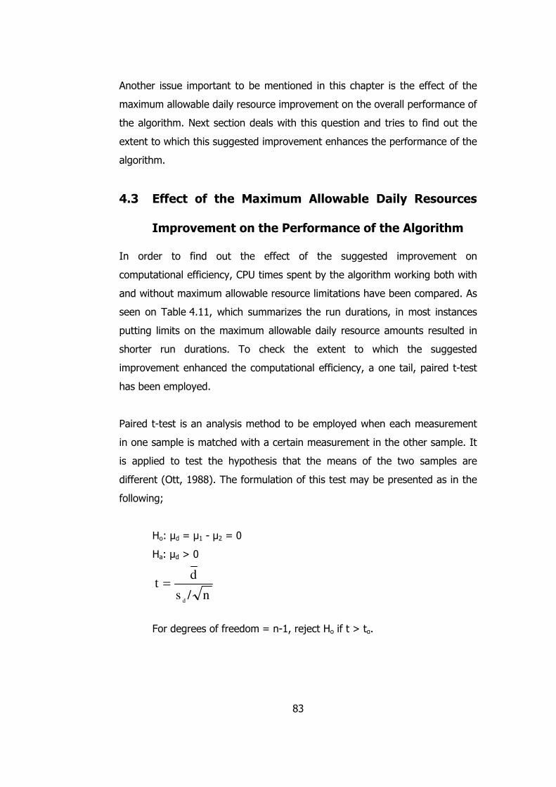
83

Another issue important to be mentioned in this chapter is the effect of the

maximum allowable daily resource improvement on the overall performance of

the algorithm. Next section deals with this question and tries to find out the

extent to which this suggested improvement enhances the performance of the

algorithm.

4.3 Effect of the Maximum Allowable Daily Resources

Improvement on the Performance of the Algorithm

In order to find out the effect of the suggested improvement on

computational efficiency, CPU times spent by the algorithm working both with

and without maximum allowable resource limitations have been compared. As

seen on Table 4.11, which summarizes the run durations, in most instances

putting limits on the maximum allowable daily resource amounts resulted in

shorter run durations. To check the extent to which the suggested

improvement enhanced the computational efficiency, a one tail, paired t-test

has been employed.

Paired t-test is an analysis method to be employed when each measurement

in one sample is matched with a certain measurement in the other sample. It

is applied to test the hypothesis that the means of the two samples are

different (Ott, 1988). The formulation of this test may be presented as in the

following;

Ho: µd = µ1 - µ2 = 0

Ha: µd > 0

For degrees of freedom = n-1, reject Ho if t > tα.

n/s

dt

d

=

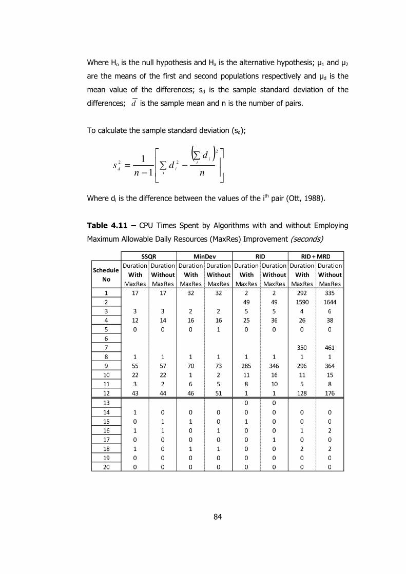
84

Where Ho is the null hypothesis and Ha is the alternative hypothesis; µ1 and µ2

are the means of the first and second populations respectively and µd is the

mean value of the differences; sd is the sample standard deviation of the

differences; is the sample mean and n is the number of pairs.

To calculate the sample standard deviation (sd);

Where di is the difference between the values of the ith pair (Ott, 1988).

Table 4.11 – CPU Times Spent by Algorithms with and without Employing

Maximum Allowable Daily Resources (MaxRes) Improvement (seconds)

Schedule

No

Duration

With

MaxRes

Duration

Without

MaxRes

Duration

With

MaxRes

Duration

Without

MaxRes

Duration

With

MaxRes

Duration

Without

MaxRes

Duration

With

MaxRes

Duration

Without

MaxRes

1 17 17 32 32 2 2 292 335

2 49 49 1590 1644

3 3 3 2 2 5 5 4 6

4 12 14 16 16 25 36 26 38

5 0 0 0 1 0 0 0 0

6

7 350 461

8 1 1 1 1 1 1 1 1

9 55 57 70 73 285 346 296 364

10 22 22 1 2 11 16 11 15

11 3 2 6 5 8 10 5 8

12 43 44 46 51 1 1 128 176

13 0 0

14 1 0 0 0 0 0 0 0

15 0 1 1 0 1 0 0 0

16 1 1 0 1 0 0 1 2

17 0 0 0 0 0 1 0 0

18 1 0 1 1 0 0 2 2

19 0 0 0 0 0 0 0 0

20 0 0 0 0 0 0 0 0

RIDMinDevSSQR RID + MRD

d

( )

∑

∑−

−=

i

ii

id

n

dd

ns

2

22

1

1

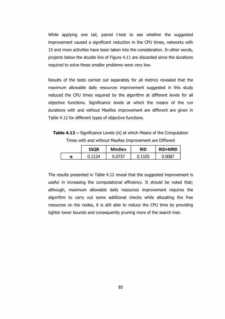
85

While applying one tail, paired t-test to see whether the suggested

improvement caused a significant reduction in the CPU times, networks with

15 and more activities have been taken into the consideration. In other words,

projects below the double line of Figure 4.11 are discarded since the durations

required to solve these smaller problems were very low.

Results of the tests carried out separately for all metrics revealed that the

maximum allowable daily resources improvement suggested in this study

reduced the CPU times required by the algorithm at different levels for all

objective functions. Significance levels at which the means of the run

durations with and without MaxRes improvement are different are given in

Table 4.12 for different types of objective functions.

Table 4.12 – Significance Levels ( ) at which Means of the Computation

Times with and without MaxRes Improvement are Different

SSQR MinDev RID RID+MRD

α 0.1124 0.0737 0.1105 0.0087

The results presented in Table 4.12 reveal that the suggested improvement is

useful in increasing the computational efficiency. It should be noted that;

although, maximum allowable daily resources improvement requires the

algorithm to carry out some additional checks while allocating the free

resources on the nodes, it is still able to reduce the CPU time by providing

tighter lower bounds and consequently pruning more of the search tree.

α

86

CHAPTER 5

CONCLUSIONS

In this study a depth-first branch and bound algorithm for solving resource

leveling problem is presented. Developed algorithm, which is applicable to

both single resource and multi resource networks, assumes no resource

availability limits and aims minimization of undesirable fluctuations in resource

distribution graphs without extending the project duration. This method is

introduced, so that more efficient schedules could be prepared to minimize all

kinds of losses due unbalanced resource distributions.

To measure undesired fluctuations in resource curves, traditional resource

leveling metrics, namely sum of squares of daily resource

requirements (SSQR) and minimum absolute deviation from the uniform

resource level (MinDev), have been utilized in addition to more recently

suggested metrics such as the resource idle day (RID). First two objective

functions have certain drawbacks that make applicability of them to

construction projects questionable. While the sum of squares metric

disregards fluctuations between consecutive time periods, minimum absolute

deviation method tries to fit resource utilization curves into rectangular

profiles, which is not very suitable to the nature of the construction projects.

Resource idle day metric, on the other hand, solely minimizes idle durations of

resources caused by resource level fluctuations and is flexible enough to deal

with unbalanced resource distributions. It is especially effective if maximum

resource demand is also minimized simultaneously as in the RID+MRD

87

objective function introduced. This metric, which is applicable for projects

which do not allow frequently releasing and rehiring resources, has been

utilized in an exact solution procedure for the first time and optimal solutions

for several problems have been reported.

Efficiency of the developed algorithm is achieved by lower bound calculation

methods adopted from the related literature and by the maximum allowable

daily resources improvement suggested for the first time in this study. Effect

of this improvement on the computational performance of the algorithm is

tested via a paired t-test based on the computational results. It is found out

that the tighter lower bounds calculated by limiting daily resource

requirements enable the algorithm to locate optimal solutions in considerably

shorter durations.

Validation of the procedure is done by solving resource leveling problems that

were available in the literature. Results obtained by the developed algorithm

are compared to the solutions of previous researchers. 3 of the addressed

problems for this purpose were solved previously via metaheuristic methods.

Developed algorithm solved these to optimality and located solutions which

have the same objective function values as reported in previous studies. In

this manner it is proved that the algorithm is capable of locating the best

known solutions for these problems so far. Moreover, the optimality of the

previously suggested solutions is also verified.

The fact that developed branch and bound algorithm finds solutions as good

as the ones reported in previous heuristic based researches signals a good

solution quality. Still, applying this type of validation only, it can not be said

that the developed procedure is always capable of locating optimal solutions.

Optimality is ensured by comparing results of the algorithm to the optimal

solutions of 8 resource leveling problems obtained via linear integer

programming. These problems are solved by a similar method to the one

88

explained in Easa (1989). Due to the limitations of the linear programming

method only MinDev metric could be utilized.

To test the computational performance of the algorithm, 20 problem instances

are solved to optimality for all of the presented metrics (i.e. SSQR, MinDev,

RID and RID+MRD) both in single and multi resource modes. CPU times and

number of search tree nodes required to ensure global optimum solution of

each problem and for each of these metrics is presented as well as the

optimum objective function values obtained. The largest single resource

network that could be solved by our algorithm included 22 activities whereas

the largest 4-resource network included 21 activities. It has been observed

that the performance of the algorithm depends on the resource leveling metric

and on the complexity of the problem under consideration. Therefore it is

difficult to estimate the problem size that can effectively be dealt via the

developed procedure. However, it can be said that resource leveling problems

with activity numbers around 20 are solvable via exact procedures.

Within the context of this study two main contributions to the existing

literature are made. Firstly, an improvement to the previously employed lower

bound calculation methods is introduced. The extent to which this maximum

allowable daily resources improvement enhanced computational performance

is determined based on the experiment results. Secondly, a problem set of 20

small size resource leveling problems has been presented and exact solutions

of these are reported in order to form a basis for performance evaluation of

heuristic studies.

As computational results indicate, CPU time required by the algorithm to reach

to the optimal solution may become relatively high in some instances. Due to

this fact, applicability of the algorithm in practice might be questionable.

Although the developed method is able to solve all kinds of networks without

requiring the user to input variables and constraints etc. as in the linear

integer programming, still the computation time may constitute a significant

89

barrier for practical purposes. Yet, rapid advances in computer technologies

have been and are going to be the major booster of exact methodologies.

There is no doubt that in the future more complex projects are going to be

solved to optimality in much shorter durations. Furthermore, exact methods

are always going to be needed since evaluation of heuristic performance

depends on the optimal solutions obtained by these methods.

As a further study, development of new and effective lower bound calculation

methods might be suggested since such improvements are believed to be the

most effective tools in enhancing the performance of branch and bound based

procedures. Also, incorporating heuristic rules or metaheuristics to the branch

and bound procedure might enhance the computational performance

significantly. Starting the search by employing such methods and obtaining a

near optimal solution in the root node could save the algorithm from visiting a

large portion of the tree by enabling it to fathom many nodes in the very

beginning of the search. In this manner, more complex problems might be

solved to optimality and developed procedure might be applied to real size

construction projects.

It is believed that carrying out experiments on a computer with larger random

access memory (RAM) would result in increased performance and would

enable solutions of more complex problems. Similarly, supercomputers with

several parallel processing units might be used to check the extent to which

new technologies enhance the computational performance. It is expected that

new technologies will reduce the CPU time requirements and eliminate stack

overflow problems to some extent enabling optimal solutions of larger

instances.

90

REFERENCES

Agin, N., (1966). “Optimum Seeking with Branch and Bound”, Management

Science, Vol. 13, No. 4, pp. B-176-B-185.

Bandelloni, M., Tucci, M. and Rinaldi, R., (1994). “Optimal Resource Leveling

Using Non-serial Dynamic Programming”, European Journal of Operational

Research, Vol. 78, Issue 2, pp. 162-177.

Bettemir, Ö. H., (2009). “Optimization of Time-Cost-Resource Trade-Off

Problems in Project Scheduling Using Meta-Heuristic Algorithms”, Middle East

Technical University, PhD. Dissertation.

Brucker, P., Knust, S., Schoo, A. and Thiele, O., (1998). “A Branch and Bound

Algorithm for the Resource-Constrained Project Scheduling Problem”,

European Journal of Operational Research, Vol. 107, pp. 272-288.

Burgess, A. R. and Killebrew, J. B., (1962). “Variation in Activity Level on a

Cyclic Arrow Diagram”, Industrial Engineering, March-April, pp. 76-83.

Çekmece, K., (2009). “The Resource Allocation Capabilities of Commercial

Project Management Software Packages for Resource Constrained Project

Scheduling Problem”, Middle East Technical University, MS. Dissertation.

Chan, W., Chua, K. H. and Kannan, G., (1996). “Construction Resource

Scheduling with Genetic Algorithms”, Journal of Construction Engineering and

Management, Vol. 122, No. 2, pp. 125-132.

91

Christodolou, S. E., Ellinas, G. and Michaelidou-Kamenou, A., (2010).

“Minimum Moment Method for Resource Leveling Using Entropy

Maximization”, Journal of Construction Engineering and Management, Vol.

136, No. 5, pp. 518-527.

De Reyck, B. and Herroelen, W., (1998). “A Branch and Bound Procedure for

the Resource-Constrained Project Scheduling Problem with Generalized

Precedence Relations”, European Journal of Operational Research, Vol. 111,

Issue 1, pp. 152-174.

Demeulemeester, E. and Herroelen, W., (1992). “A Branch-and-Bound

Procedure for the Multiple Resource-Constrained Project Scheduling Problem”,

Management Science, Vol. 38, No. 12, pp. 1803-1818.

Demeulemeester, E., (1995). “Minimizing Resource Availability Costs in Time-

Limited Project Networks”, Management Science, Vol. 41, No. 10, pp. 1590-

1598.

Demeulemeester, E. and Herroelen, W., (1997). “A Branch-and-Bound

Procedure for the Generalized Resource-Constrained Project Scheduling

Problem”, Operations Research, Vol. 45, No. 2, pp. 201-212.

Demeulemeester, E. and Herroelen, W., (2002). “Project Scheduling: A

Research Handbook”, Kluwer Academic Publishers, Boston.

Easa, S., (1989). “Resource Leveling in Construction by Optimization”. Journal

of Construction Engineering and Management, Vol. 115, No. 2, pp. 302-316.

El-Rayes, K. and Jun, D. H., (2009). “Optimizing Resource Leveling in

Construction Projects”, Journal of Construction Engineering and Management,

Vol. 135, No. 11, pp. 1172-1180.

92

Guo, Y., Li, N., Ye, T., (2009). “Multiple Resources Leveling in Multiple

Projects Scheduling Problem Using Particle Swarm Optimization”, Fifth

International Conference on Natural Computation, pp. 260-264.

Harris, R. B., (1990). “Packing Method for Resource Leveling (PACK)”, Journal

of Construction Engineering and Management, Vol. 116, No. 2, pp. 331-350.

Hegazy, T., (1999). “Optimization of Resource Allocation and Leveling Using

Genetic Algorithms”, Journal of Construction Engineering and Management,

Vol. 125, No. 3, pp. 167-175.

Herroelen, W., (2005). “Project Scheduling – Theory and Practice”, Production

and Operations Management, Vol. 14, No. 4, pp. 413-432.

Hinze, J. W., (2004). “Construction Planning and Scheduling”, Pearson

Prentice Hall, Upper Saddle River, New Jersey.

Hiyassat, M. A. S., (2000). “Modification of Minimum Moment Approach In

Resource Leveling”, Journal of Construction Engineering and Management,

Vol. 126, No. 4, pp. 278-284.

Hiyassat, M. A. S., (2001). “Applying Modified Minimum Moment Method to

Multiple Resource Leveling”, Journal of Construction Engineering and

Management, Vol. 127, No.3, pp. 192-198.

Icmeli, O. and Erenguc, S. S., (1996). “A Branch and Bound Procedure for the

Resource Constrained Project Scheduling Problem with Discounted Cash

Flows”, Management Science, Vol. 42, No. 10, pp. 1395-1408.

93

Jiang, G. and Shi, J., (2005). “Exact Algorithm for Solving Project Scheduling

Problems under Multiple Resource Constraints”, Journal of Construction

Engineering and Management, Vol. 131, No. 9, pp. 986-992.

Karshenas, S. and Haber, D., (1990). “Economic Optimization of Construction

Project Scheduling”, Construction Management and Economics, Vol. 8, pp.

135-146.

Leu, S. and Yang, C., (1999). “GA-Based Multicriteria Optimal Model for

Construction Scheduling”, Journal of Construction Engineering and

Management, Vol. 125, No. 6, pp. 420-427.

Leu, S., Yang, C. and Huang, J., (2000). “Resource Leveling in Construction by

Genetic Algorithm-Based Optimization and Its Decision Support System

Application”, Automation in Construction, Vol. 10, pp. 27-41.

Martinez, J. and Ioannou, P., (1993). “Resource Leveling Based on the

Modified Minimum Moment Heuristic”, Computing in Civil and Building

Engineering, Conference Proceeding Paper, pp. 287-294.

Mason, A. T. and Moodie, C. L., (1971). “A Branch and Bound Algorithm for

Minimizing Cost in Project Scheduling”, Management Science, Vol. 18, No. 4,

pp. B-158-B-173.

Mattila, K. G. and Abraham, D. M., (1998). “Resource Leveling of Linear

Schedules Using Integer Linear Programming”, Journal of Construction


Mubarak, S. A., (2004). “Construction Project Scheduling and Control”,

Pearson Prentice Hall, Upper Saddle River, New Jersey.

94

Neumann, K. and Zimmermann, J., (1999). “Resource Levelling for Projects

with Schedule-Dependent Time Windows”, European Journal of Operational

Research, Vol. 117, pp. 591-605.

Neumann, K. and Zimmermann, J., (2000). “Procedures for Resource Leveling

and Net Present Value Problems in Project Scheduling with General Temporal

and Resource Constraints”, European Journal of Operational Research, Vol.

127, pp. 425-443.

Newitt, J. S., (2005). “Construction Scheduling: Principles and Practices”,

Pearson Prentice Hall, Upper Saddle River, New Jersey.

Oral, M., Laptalı Oral, E., Bozkurt, S. and Erdiş, E, (2003). “Resource Leveling

in Construction Projects by Using Genetic Algorithms”, Ç. Ü. J. Fac. Eng. Arch,

Vol. 18, No. 2, pp. 185-194.

Ott, L., (1988). “An Introduction to Statistical Methods and Data Analysis”,

PWS-KENT Publishing Company, Boston.

Pang, N., Shi, Y. and You, Y., (2008). “Resource Leveling Optimization of

Network Schedule Based on Particle Swarm Optimization with Constriction

Factor”, International Conference on Advanced Computer Theory and

Engineering, pp.652-656.

Patterson, J. H., (1984). “A Comparison of Exact Approaches for Solving the

Multiple Constrained Resource, Project Scheduling Problem”, Management

Science, Vol. 30, No. 7, pp. 854-867.

Savin, D., Alkass, S. and Fazio, P., (1996). “Construction Resource Leveling

Using Neural Networks”, Canadian Journal of Civil Engineering, Vol. 23,

Issue 4, pp. 917-925.

95

Senouci, A. B. and Eldin, N. N., (2004). “Use of Genetic Algorithms in

Resource Scheduling of Construction Projects”, Journal of Construction


Shah, K. A., Farid, F. and Baugh, J. W., Jr. (1993). “Optimal Resource Leveling

Using Integer Linear Programming”, Proceedings 4th International Conference

on Computing in Civil and Building Engineering, pp. 501-508.

Son, J. and Skibniewski, M. J., (1999). “Multiheuristic Approach for Resource

Leveling Problem in Construction Engineering: Hybrid Approach”, Journal of

Construction Engineering and Management, Vol. 125, No. 1, pp. 23-31.

Son, J. and Mattila, K. G., (2004). “Binary Resource Leveling Model: Activity

Splitting Allowed”, Journal of Construction Engineering and Management, Vol.

130, No. 6, pp. 887-894.

Stevens, J. D., (1990). “Techniques for Construction Network Scheduling”, Mc

Graw-Hill, New York.

Vanhoucke, M., Demeulemeester, E. And Herroelen, W., (2001). “On

Maximizing the Net Present Value of a Project under Renewable Resource

Constraints”, Management Science, Vol. 47, No. 8, pp. 1113-1121.

Woodworth, M. W. and Willie, C. J., (1975). “A Heuristic Algorithm for

Resource Leveling in Multi-Project, Multi-Resource Scheduling”, Decision

Sciences, Vol. 6, Issue 3, pp. 525-540.

Younis, M. A. and Saad, B., (1996). “Optimal Resource Leveling of Multi-

Resource Projects”, Computers and Industrial Engineering, Vol. 31, Issue 1,2,

pp. 1-4.

96

Zheng, D. X. M., Ng S. T. and Kumaraswamy, M. M., (2003), ASCE

Construction Research Congress, pp. 1-8.

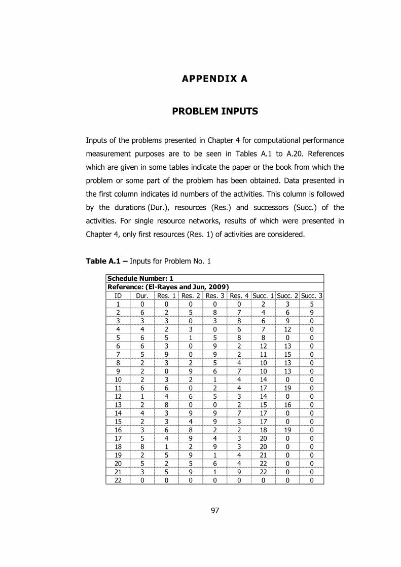
97

APPENDIX A

PROBLEM INPUTS

Inputs of the problems presented in Chapter 4 for computational performance

measurement purposes are to be seen in Tables A.1 to A.20. References

which are given in some tables indicate the paper or the book from which the

problem or some part of the problem has been obtained. Data presented in

the first column indicates id numbers of the activities. This column is followed

by the durations (Dur.), resources (Res.) and successors (Succ.) of the

activities. For single resource networks, results of which were presented in

Chapter 4, only first resources (Res. 1) of activities are considered.

Table A.1 – Inputs for Problem No. 1

ID Dur. Res. 1 Res. 2 Res. 3 Res. 4 Succ. 1 Succ. 2 Succ. 31 0 0 0 0 0 2 3 52 6 2 5 8 7 4 6 93 3 3 0 3 8 6 9 04 4 2 3 0 6 7 12 05 6 5 1 5 8 8 0 06 6 3 0 9 2 12 13 07 5 9 0 9 2 11 15 08 2 3 2 5 4 10 13 09 2 0 9 6 7 10 13 010 2 3 2 1 4 14 0 011 6 6 0 2 4 17 19 012 1 4 6 5 3 14 0 013 2 8 0 0 2 15 16 014 4 3 9 9 7 17 0 015 2 3 4 9 3 17 0 016 3 6 8 2 2 18 19 017 5 4 9 4 3 20 0 018 8 1 2 9 3 20 0 019 2 5 9 1 4 21 0 020 5 2 5 6 4 22 0 021 3 5 9 1 9 22 0 022 0 0 0 0 0 0 0 0

Reference: (El-Rayes and Jun, 2009)

Schedule Number: 1

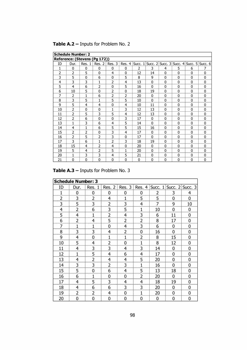
98


ID Dur. Res. 1 Res. 2 Res. 3 Res. 4 Succ. 1 Succ. 2 Succ. 3 Succ. 4 Succ. 5 Succ. 61 0 0 0 0 0 2 3 4 5 6 72 2 5 0 4 0 12 14 0 0 0 03 5 0 6 0 5 8 9 0 0 0 04 3 3 1 2 4 13 0 0 0 0 05 4 6 2 0 5 16 0 0 0 0 06 10 5 0 2 0 18 19 0 0 0 07 2 1 6 2 2 20 0 0 0 0 08 3 5 1 5 5 10 0 0 0 0 09 5 4 4 0 4 10 11 0 0 0 010 2 0 0 1 3 12 13 0 0 0 011 2 5 3 5 4 12 13 0 0 0 012 2 6 0 0 3 17 0 0 0 0 013 1 3 6 4 5 14 0 0 0 0 014 4 1 6 5 5 15 16 0 0 0 015 2 2 0 3 4 17 0 0 0 0 016 2 5 2 3 0 17 0 0 0 0 017 3 6 1 2 3 18 19 0 0 0 018 15 4 2 4 0 20 0 0 0 0 019 5 4 2 5 1 20 0 0 0 0 020 1 3 3 4 5 21 0 0 0 0 021 0 0 0 0 0 0 0 0 0 0 0

Reference: (Stevens (Pg 172))

Schedule Number: 2


ID Dur. Res. 1 Res. 2 Res. 3 Res. 4 Succ. 1 Succ. 2 Succ. 31 0 0 0 0 0 2 3 42 3 2 4 1 5 5 0 03 5 3 2 3 4 7 9 104 2 6 3 5 1 10 0 05 4 1 2 4 3 6 11 06 2 4 5 2 2 8 17 07 1 1 0 4 3 6 0 08 3 3 4 2 0 16 0 09 4 0 1 1 2 8 15 010 5 4 2 0 1 8 12 011 4 3 3 4 3 14 0 012 1 5 4 6 4 17 0 013 4 2 4 4 5 20 0 014 3 3 2 3 1 16 0 015 5 0 6 4 5 13 18 016 6 1 0 0 2 20 0 017 4 5 3 4 4 18 19 018 4 6 6 3 3 20 0 019 2 2 4 0 1 20 0 020 0 0 0 0 0 0 0 0

Schedule Number: 3

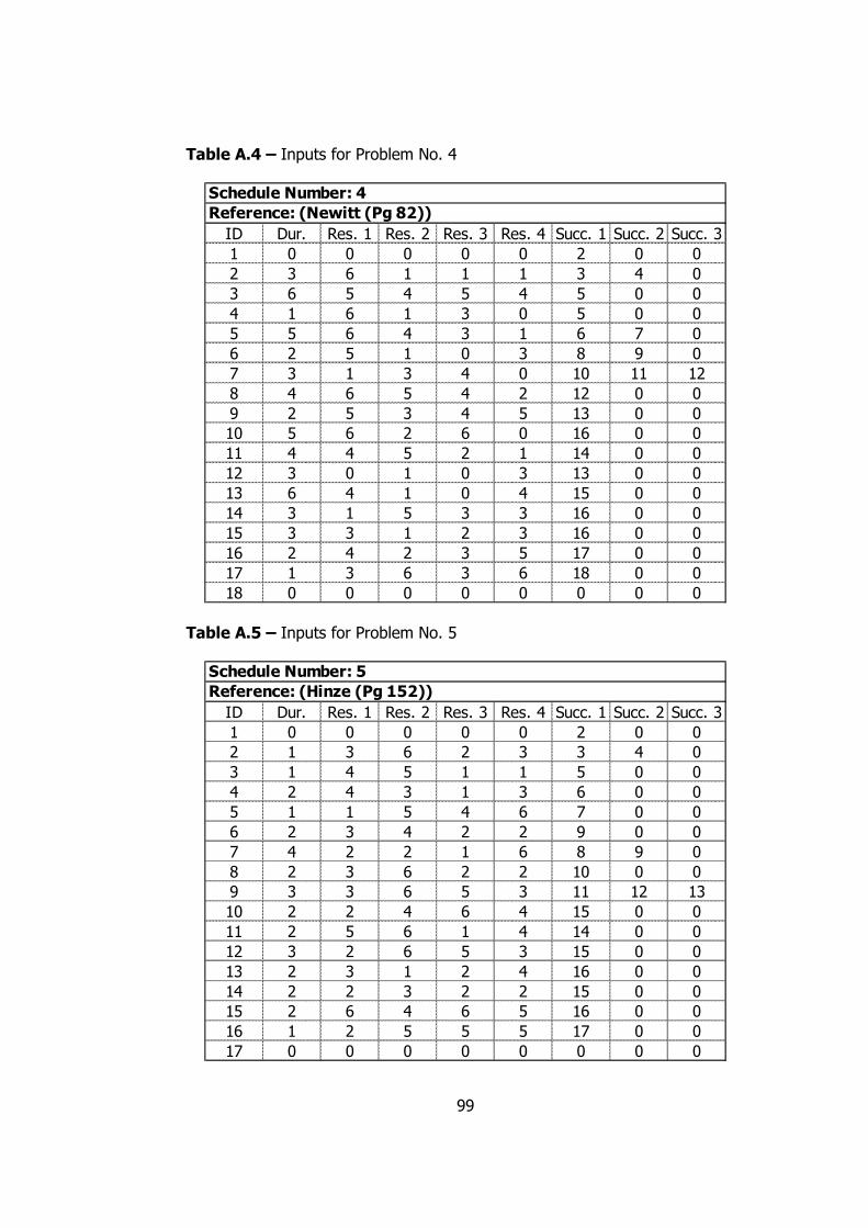
99


ID Dur. Res. 1 Res. 2 Res. 3 Res. 4 Succ. 1 Succ. 2 Succ. 31 0 0 0 0 0 2 0 02 3 6 1 1 1 3 4 03 6 5 4 5 4 5 0 04 1 6 1 3 0 5 0 05 5 6 4 3 1 6 7 06 2 5 1 0 3 8 9 07 3 1 3 4 0 10 11 128 4 6 5 4 2 12 0 09 2 5 3 4 5 13 0 010 5 6 2 6 0 16 0 011 4 4 5 2 1 14 0 012 3 0 1 0 3 13 0 013 6 4 1 0 4 15 0 014 3 1 5 3 3 16 0 015 3 3 1 2 3 16 0 016 2 4 2 3 5 17 0 017 1 3 6 3 6 18 0 018 0 0 0 0 0 0 0 0

Schedule Number: 4

Reference: (Newitt (Pg 82))


ID Dur. Res. 1 Res. 2 Res. 3 Res. 4 Succ. 1 Succ. 2 Succ. 31 0 0 0 0 0 2 0 02 1 3 6 2 3 3 4 03 1 4 5 1 1 5 0 04 2 4 3 1 3 6 0 05 1 1 5 4 6 7 0 06 2 3 4 2 2 9 0 07 4 2 2 1 6 8 9 08 2 3 6 2 2 10 0 09 3 3 6 5 3 11 12 1310 2 2 4 6 4 15 0 011 2 5 6 1 4 14 0 012 3 2 6 5 3 15 0 013 2 3 1 2 4 16 0 014 2 2 3 2 2 15 0 015 2 6 4 6 5 16 0 016 1 2 5 5 5 17 0 017 0 0 0 0 0 0 0 0

Schedule Number: 5

Reference: (Hinze (Pg 152))

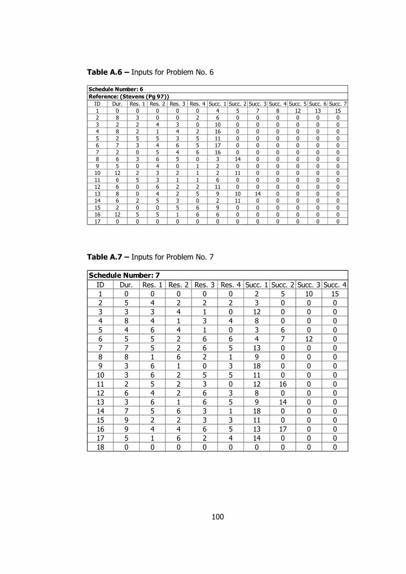
100


ID Dur. Res. 1 Res. 2 Res. 3 Res. 4 Succ. 1 Succ. 2 Succ. 3 Succ. 4 Succ. 5 Succ. 6 Succ. 71 0 0 0 0 0 4 5 7 8 12 13 152 8 3 0 0 2 6 0 0 0 0 0 03 2 2 4 3 0 10 0 0 0 0 0 04 8 2 1 4 2 16 0 0 0 0 0 05 2 5 5 3 5 11 0 0 0 0 0 06 7 3 4 6 5 17 0 0 0 0 0 07 2 0 5 4 6 16 0 0 0 0 0 08 6 3 6 5 0 3 14 0 0 0 0 09 5 0 4 0 1 2 0 0 0 0 0 010 12 2 3 2 1 2 11 0 0 0 0 011 6 5 3 1 1 6 0 0 0 0 0 012 6 0 6 2 2 11 0 0 0 0 0 013 8 0 4 2 5 9 10 14 0 0 0 014 6 2 5 3 0 2 11 0 0 0 0 015 2 0 0 5 6 9 0 0 0 0 0 016 12 5 5 1 6 6 0 0 0 0 0 017 0 0 0 0 0 0 0 0 0 0 0 0

Schedule Number: 6

Reference: (Stevens (Pg 97))


ID Dur. Res. 1 Res. 2 Res. 3 Res. 4 Succ. 1 Succ. 2 Succ. 3 Succ. 41 0 0 0 0 0 2 5 10 152 5 4 2 2 2 3 0 0 03 3 3 4 1 0 12 0 0 04 8 4 1 3 4 8 0 0 05 4 6 4 1 0 3 6 0 06 5 5 2 6 6 4 7 12 07 7 5 2 6 5 13 0 0 08 8 1 6 2 1 9 0 0 09 3 6 1 0 3 18 0 0 010 3 6 2 5 5 11 0 0 011 2 5 2 3 0 12 16 0 012 6 4 2 6 3 8 0 0 013 3 6 1 6 5 9 14 0 014 7 5 6 3 1 18 0 0 015 9 2 2 3 3 11 0 0 016 9 4 4 6 5 13 17 0 017 5 1 6 2 4 14 0 0 018 0 0 0 0 0 0 0 0 0

Schedule Number: 7

101


ID Dur. Res. 1 Res. 2 Res. 3 Res. 4 Succ. 1 Succ. 2 Succ. 31 0 0 0 0 0 2 0 02 2 2 5 6 3 3 4 53 7 0 3 2 4 6 7 04 10 3 1 6 2 7 8 05 4 0 4 0 2 8 9 06 6 2 1 2 3 12 0 07 5 1 5 6 6 10 11 148 8 4 4 2 4 10 13 09 9 3 3 6 3 13 14 010 12 5 6 6 5 15 0 011 5 5 0 0 0 12 0 012 5 3 5 3 0 15 0 013 6 2 5 4 5 15 0 014 4 1 1 3 6 15 0 015 3 3 4 4 5 16 0 016 0 0 0 0 0 0 0 0

Schedule Number: 8

Reference: (Mubarak (Pg 61))



Schedule Number: 9

102



Schedule Number: 10


ID Dur. Res. 1 Res. 2 Res. 3 Res. 4 Succ. 1 Succ. 2 Succ. 31 0 0 0 0 0 2 4 02 5 2 1 6 6 3 0 03 8 3 6 6 2 8 0 04 2 3 6 4 0 5 9 05 1 5 6 3 6 3 6 106 4 3 3 6 3 11 0 07 2 1 6 6 2 8 0 08 7 2 1 4 2 15 0 09 4 3 2 1 5 10 13 010 3 2 4 3 3 7 0 011 1 1 0 5 6 8 0 012 4 6 4 5 1 15 0 013 2 4 4 3 0 11 14 014 3 3 4 0 1 12 0 015 0 0 0 0 0 0 0 0

Schedule Number: 11

103


ID Dur. Res. 1 Res. 2 Res. 3 Res. 4 Succ. 1 Succ. 21 0 0 0 0 0 2 32 5 6 7 5 7 4 03 10 3 4 2 3 5 64 10 5 2 4 7 7 85 5 4 9 1 1 9 06 5 6 0 3 9 10 117 10 4 4 5 0 12 08 5 7 4 2 5 13 09 10 0 3 9 4 13 010 5 5 5 3 6 13 011 10 6 6 0 4 14 012 5 8 2 2 0 14 013 10 8 5 2 7 14 014 5 9 5 0 4 15 015 0 0 0 0 0 0 0

Schedule Number: 12

Reference: (Son and Skibniewski, 1999)


ID Dur. Res. 1 Res. 2 Res. 3 Res. 4 Succ. 1 Succ. 2 Succ. 3 Succ. 4 Succ. 51 0 0 0 0 0 2 0 0 0 02 3 15 7 4 8 3 4 5 6 73 3 6 12 11 11 8 0 0 0 04 8 12 5 15 0 9 10 0 0 05 2 10 6 11 4 11 0 0 0 06 4 15 4 7 10 14 0 0 0 07 6 10 2 8 8 14 0 0 0 08 3 7 1 13 4 14 0 0 0 09 5 12 11 13 6 12 0 0 0 010 2 6 10 7 4 13 0 0 0 011 2 10 13 11 7 13 0 0 0 012 3 14 12 4 13 14 0 0 0 013 2 8 14 6 8 14 0 0 0 014 2 10 5 4 5 15 0 0 0 015 0 0 0 0 0 0 0 0 0 0

Schedule Number: 13

Reference: (Leu, Yang and Huang, 2000)

104


ID Dur. Res. 1 Res. 2 Res. 3 Res. 4 Succ. 1 Succ. 2 Succ. 3 Succ. 41 0 0 0 0 0 2 0 0 02 4 4 2 1 6 3 4 0 03 2 2 4 0 3 11 0 0 04 5 6 0 3 6 8 0 0 05 2 0 0 5 1 10 0 0 06 2 6 6 0 0 12 0 0 07 5 2 5 6 6 12 0 0 08 7 4 6 6 6 5 6 7 99 3 6 1 0 3 12 0 0 010 2 3 0 6 6 11 0 0 011 4 5 5 2 3 13 0 0 012 3 1 4 5 6 13 0 0 013 21 0 5 4 2 14 0 0 014 0 0 0 0 0 0 0 0 0

Schedule Number: 14

Reference: (Newitt (Pg 121))


ID Dur. Res. 1 Res. 2 Res. 3 Res. 4 Succ. 1 Succ. 2 Succ. 31 0 0 0 0 0 2 3 42 2 2 6 4 4 5 6 03 4 1 2 2 1 6 7 04 1 4 1 6 4 7 8 05 4 4 4 3 2 9 0 06 3 2 5 6 2 9 10 07 6 4 3 6 3 11 0 08 6 6 4 6 0 10 11 09 1 0 2 5 1 12 0 010 4 2 1 0 6 12 0 011 5 1 1 3 3 12 0 012 1 2 6 3 2 13 0 013 0 0 0 0 0 0 0 0

Schedule Number: 15

Reference: (Harris, 1990)

105


ID Dur. Res. 1 Res. 2 Res. 3 Res. 4 Succ. 1 Succ. 21 0 0 0 0 0 2 102 8 2 0 5 4 3 03 3 3 2 1 4 5 04 3 3 1 1 1 8 05 5 3 2 4 3 13 06 3 2 1 2 5 5 07 3 4 1 1 3 6 48 4 4 3 1 0 9 09 3 4 0 1 1 13 010 6 3 3 0 3 7 1111 5 3 4 4 2 12 012 5 3 3 5 2 8 013 0 0 0 0 0 0 0

Schedule Number: 16

Reference: (Son and Skibniewski, 1999)


ID Dur. Res. 1 Res. 2 Res. 3 Res. 4 Succ. 1 Succ. 2 Succ. 31 0 0 0 0 0 2 0 02 2 2 4 6 2 3 4 03 5 5 4 3 3 5 6 74 6 0 2 4 1 7 8 05 6 1 1 6 6 9 11 06 7 5 2 5 0 9 10 07 4 3 2 4 5 9 10 08 5 2 6 2 2 10 0 09 10 5 5 5 1 12 0 010 8 5 0 5 3 12 0 011 7 0 1 1 1 12 0 012 1 3 4 6 6 13 0 013 0 0 0 0 0 0 0 0

Schedule Number: 17


106


ID Dur. Res. 1 Res. 2 Res. 3 Res. 4 Succ. 1 Succ. 2 Succ. 3 Succ. 4 Succ. 5 Succ. 61 0 0 0 0 0 2 3 4 5 6 72 7 7 4 4 0 8 0 0 0 0 03 7 4 4 3 1 8 0 0 0 0 04 5 2 0 6 3 9 0 0 0 0 05 9 3 1 1 0 9 0 0 0 0 06 4 5 4 5 6 12 0 0 0 0 07 2 4 6 2 5 10 0 0 0 0 08 9 2 3 6 3 12 0 0 0 0 09 5 5 0 2 5 12 0 0 0 0 010 3 3 5 2 0 11 0 0 0 0 011 7 6 6 5 0 12 0 0 0 0 012 0 0 0 0 0 0 0 0 0 0 0

Reference: (Demeulemeester (Pg 416))

Schedule Number: 18


ID Dur. Res. 1 Res. 2 Res. 3 Res. 4 Succ. 1 Succ. 2 Succ. 31 0 0 0 0 0 2 0 02 5 1 3 1 1 3 4 53 7 2 1 4 5 6 0 04 8 4 0 5 5 6 7 05 11 5 2 3 0 8 0 06 6 6 3 3 4 9 0 07 4 1 6 1 6 8 9 08 7 4 2 2 6 10 0 09 6 0 3 6 0 10 0 010 0 0 0 0 0 0 0 0

Schedule Number: 19



ID Dur. Res. 1 Res. 2 Res. 3 Res. 4 Succ. 1 Succ. 2 Succ. 31 0 0 0 0 0 2 4 62 12 3 2 4 3 8 0 03 2 5 6 2 4 8 0 04 5 6 1 5 2 3 5 05 6 2 4 2 2 8 0 06 6 4 4 1 7 7 0 07 1 8 1 4 1 3 0 08 0 0 0 0 0 0 0 0

Schedule Number: 20

Documents

A BRANCH AND BOUND ALGORITHM FOR … · a branch and bound algorithm for resource leveling problem a thesis submitted to the graduate school of natural and applied sciences of middle