1

A Binary Linear Programming Formulation of

the Graph Edit Distance

Derek Justice and Alfred Hero

Department of Electrical Engineering and Computer Science

University of Michigan

Ann Arbor, MI 48109

Abstract

A binary linear programming formulation of the graph edit distance for unweighted, undirected

graphs with vertex attributes is derived and applied to a graph recognition problem. A general formulation

for editing graphs is used to derive a graph edit distance that is proven to be a metric provided the

cost function for individual edit operations is a metric. Then, a binary linear program is developed

for computing this graph edit distance, and polynomial time methods for determining upper and lower

bounds on the solution of the binary program are derived by applying solution methods for standard

linear programming and the assignment problem. A recognition problem of comparing a sample input

graph to a database of known prototype graphs in the context of a chemical information system is

presented as an application of the new method. The costs associated with various edit operations are

chosen by using a minimum normalized variance criterion applied to pairwise distances between nearest

neighbors in the database of prototypes. The new metric is shown to perform quite well in comparison

to existing metrics when applied to a database of chemical graphs.

Index Terms

Graph algorithms, Similarity measures, Structural Pattern Recognition, Graphs and Networks, Linear

Programming, Continuation (homotopy) methods

2

I. I NTRODUCTION

Attributed graphs provide convenient structures for representing objects when relational prop-

erties are of interest. Such representations are frequently useful in applications ranging from

computer-aided drug design to machine vision. A familiar machine vision problem is to recognize

specific objects within an image. In this case, the image is processed to generate a representative

graph based on structural characteristics, such a region adjacency graph or a line adjacency graph,

and vertex attributes may be assigned according to characteristics of the region to which each

vertex corresponds [1]. This representative graph is then compared to a database of prototype

or model graphs in order to identify and classify the object of interest. Face identification [2]

and symbol recognition [3] are among the problems in machine vision where graphs have been

utilized recently. In this context, a reliable and speedy method for comparing graphs is important.

Many heuristics and simplifications have been developed and employed for this purpose in a

variety of applications [4].

Comparing graphs in the context of graph database searching has also found significant

application in the pharmaceutical and agrochemical industries. The attributed graphs of interest

are so called chemical graphs which are derived from chemical structure diagrams. Graphical

representations are of great utility here because of thesimilar property principle, which states

that molecules with similar structures will exhibit similar chemical properties [5]. Thus databases

of these chemical graphs are often searched by comparing with a query graph to aid in the design

of new chemicals or medicines [6]. Various techniques have been designed for processing the

graphs for structural features and generating bit strings (referred to asfingerprints) based on the

presence or absence of such features [7]. Since the fingerprints can be rapidly compared, some

pre-screening or clustering is often done based on these to eliminate all but the most similar

graphs to a given input graph. The remaining graphs may then be compared to the query using

a more sophisticated (and more computationally demanding) method. Distance metrics based on

the maximum common subgraph are frequently used in this role [8], [9].

Although computing the maximum common subgraph (MCS) is no small task (indeed, it is

an NP-Hard problem [10]), several graph distance metrics have been proposed that use the size

3

of the MCS. One such metric is given in [11], with a slight modification presented in [12]. A

different MCS-based metric is presented in [13] specifically for application to chemical graphs.

An alternate metric that uses the MCS along with the minimum common supergraph has also

been proposed [14]. For related structures, such as attributed trees, it is often possible to derive

distance metrics based on the maximum common substructure that operate in polynomial time

[15]. An intimate relationship between graph comparison and graph (or subgraph) isomorphism

is readily apparent in these examples because the MCS defines subgraphs in the two graphs

being compared that are isomorphic. Indeed, computing a graph distance metric often requires

the computation of some sort of isomorphism (aka matching) between graphs.

An exact graph isomorphism defines a mapping between the nodes of two attributed graphs so

that their structures (vertex attributes along with edges) exactly coincide. As one might expect,

this is also a challenging computational problem in general although it has not been shown to

be NP-Complete [10]. As with subgraph isomorphism, polynomial time algorithms are available

for certain restricted classes of graphs [16]. Algorithms for general graph isomorphism that

are shown to be quite speedy in practice are given in [17], [18]. Such algorithms typically

take advantage of vertex attributes to efficiently prune a search tree constructed for finding an

isomorphism. Graphs obtained from real objects are rarely isomorphic, however, so it is useful to

consider inexact or error-correcting graph isomorphisms (ECGI) that allow for graphs to nearly

(but not exactly) coincide [19]. As the name suggests, the lack of exact isomorphism can be

caused by measurement noise or errors in a sample graph when compared to a model graph. On

the other hand, when comparing two model graphs one might interpret such ’errors’ as capturing

the essential differences between the two graphs.

Error-correcting graph matching attempts to compute a mapping between the vertices of two

graphs so that they approximately coincide, realizing that the graphs may not be isomorphic.

Many suboptimal approaches exist to tackle this problem [20], [21], [22], [23]. The adjacency

matrix eigendecomposition approach of [21] gives fast suboptimal results, however it is only

applicable to graphs having adjacency matrices with no repeated eigenvalues. Graphs with a

low degree of connectivity will often have adjacency matrices with multiple zero eigenvalues.

4

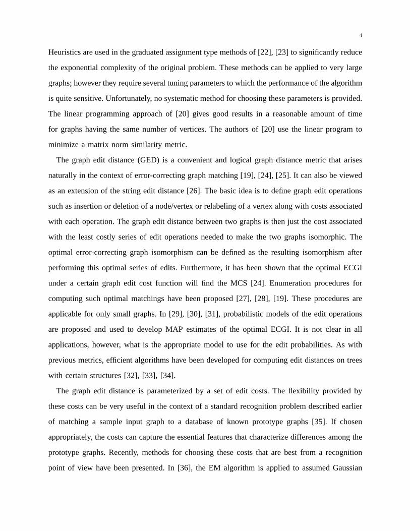
Heuristics are used in the graduated assignment type methods of [22], [23] to significantly reduce

the exponential complexity of the original problem. These methods can be applied to very large

graphs; however they require several tuning parameters to which the performance of the algorithm

is quite sensitive. Unfortunately, no systematic method for choosing these parameters is provided.

The linear programming approach of [20] gives good results in a reasonable amount of time

for graphs having the same number of vertices. The authors of [20] use the linear program to

minimize a matrix norm similarity metric.

The graph edit distance (GED) is a convenient and logical graph distance metric that arises

naturally in the context of error-correcting graph matching [19], [24], [25]. It can also be viewed

as an extension of the string edit distance [26]. The basic idea is to define graph edit operations

such as insertion or deletion of a node/vertex or relabeling of a vertex along with costs associated

with each operation. The graph edit distance between two graphs is then just the cost associated

with the least costly series of edit operations needed to make the two graphs isomorphic. The

optimal error-correcting graph isomorphism can be defined as the resulting isomorphism after

performing this optimal series of edits. Furthermore, it has been shown that the optimal ECGI

under a certain graph edit cost function will find the MCS [24]. Enumeration procedures for

computing such optimal matchings have been proposed [27], [28], [19]. These procedures are

applicable for only small graphs. In [29], [30], [31], probabilistic models of the edit operations

are proposed and used to develop MAP estimates of the optimal ECGI. It is not clear in all

applications, however, what is the appropriate model to use for the edit probabilities. As with

previous metrics, efficient algorithms have been developed for computing edit distances on trees

with certain structures [32], [33], [34].

The graph edit distance is parameterized by a set of edit costs. The flexibility provided by

these costs can be very useful in the context of a standard recognition problem described earlier

of matching a sample input graph to a database of known prototype graphs [35]. If chosen

appropriately, the costs can capture the essential features that characterize differences among the

prototype graphs. Recently, methods for choosing these costs that are best from a recognition

point of view have been presented. In [36], the EM algorithm is applied to assumed Gaussian

5

mixture models for edit events in order to choose costs that enforce similarity (or dissimilarity)

between specific pairs of graphs in a training set. An application for matching images based on

their shock graphs [37] uses the tree edit distance algorithm in [34] and chooses edit costs based

on local shape differences within shock graphs corresponding to similar images. In a chemical

graph recognition application, heuristics are used to choose the edit costs of a string edit distance

between strings formed from the maximal paths between vertices in the graphs [38]. Related

studies have also been done into the effectiveness of weighting the presence or absence of certain

substructures differently when comparing fingerprints derived from chemical graphs [39].

In this paper, we provide a formulation of the graph edit distance whereby error-correcting

graph matching may be performed by solving a binary linear program (BLP–that is a linear

program where all variables must take values from the set0, 1). We first present a general

framework for computing the GED between attributed, unweighted graphs by treating them as

subgraphs of a larger graph referred to as the edit grid. It is argued that the edit grid need only

have as many vertices as the sum of the total number of vertices in the graphs being compared.

We show that graph editing is equivalent to altering the state of the edit grid and prove that the

GED derived in this way is a metric provided the cost function for individual edit operations is

a metric. We then use the adjacency matrix representation to formulate a binary linear program

to solve for the GED. Since solving a BLP is NP-Hard [10], we show how to obtain upper and

lower bounds for the GED in polynomial time by using solution techniques for standard linear

programming and the assignment problem [40]. These bounds may be useful in the event that

the problem is so large that solving the BLP is impractical.

We also present a recognition problem [35] that demonstrates the utility of the new method in

the context of a chemical information system. Suppose there is a database of prototype chemical

graphs to which a sample graph is to be compared as described earlier. The experiment proceeds

in two stages: edit cost selection followed by recognition of a perturbed prototype graph via

a minimum distance classifier. We provide a method for choosing the edit costs that is purely

nonparametric and is based on the assumption (or prior information) that the graphs in the

database should be uniformly distributed. The edit costs are chosen as those that minimize

6

the normalized variance of pairwise distances between nearest neighbor prototypes, thereby

uniformly distributing them in the metric space of graphs define by the GED. Note that a metric

which uniformly distributes nearest neighbors in the database essentially equalizes the probability

of classification error with a minimum distance classifier, thereby minimizing the worst case error.

This method is similar to the use of spherical packings for error-correcting code design, where

the distances between all nearest-neighbor code points are the same [41]. Also, providing such

homogeneous sets of graphs is desirable in chemical applications for certain structure-activity

experiments [6]. This computation involves matching all pairs of prototypes in a neighborhood

and tabulating the edits between them. These are provided as inputs to a single convex program

to solve for the optimal edit costs. This is one possible method for choosing edit costs; other

methods might certainly be concocted to accommodate whatever prior information about the

data at hand is available.

We test our algorithm on a database of 135 chemical graphs derived from a set of similar

biochemical molecules [42]. Our GED metric is compared with the MCS based metrics proposed

in [13], [11]. Indeed, the similarity of molecules in this database indicates it is a good candidate

for our method of edit cost selection. We first compute the optimal edit costs as previously

described and show that our metric equipped with these costs more uniformly distributes the

prototype graphs than either MCS metric. The recognition problem is investigated next by

generating sample graphs through random perturbations on the prototype graphs; thus we consider

a scenario where the ECGI is used to ’fix’ errors between sample and model graphs. Each sample

graph is matched to every prototype in the database in an effort to recognize which prototype

was perturbed to create the sample graph, and a classification ambiguity index is computed.

The GED metric is found to perform better with respect to certain types of edit and worse with

respect to others than the MCS metrics. However, when random edits are applied, the GED

typically performs better.

This paper is organized as follows. Section II presents the bulk of the theory. Within Section

II, we first present the general framework for computing the GED and prove that it results

in a metric provided the edit cost function is a metric. This is followed by the development

7

of the binary linear program to compute the graph edit distance along with a description of

polynomial-time solutions for upper and lower bounds on the GED. Finally a description of

edit cost selection for a graph recognition problem is given, and it is shown that the resulting

problem is a convex program. Section III presents the results of the graph recognition problem

applied to a database of chemical graphs, and Section IV provides some concluding remarks.

II. T HEORY

We first introduce a framework for edits on the set of unweighted, undirected graphs with

vertex attributes based on relabeling of graph elements (vertices and edges). Suppose we wish to

find the graph edit distance between graphsG0 andG1. The graph to be editedG0 is embedded

in a labeled complete graphGΩ referred to as the ’edit grid.’ Vertices and edges inGΩ may

possess the special null label indicating the element is not part of the embedded graph; such an

element is referred to as ’virtual’ and allows for insertion and deletion edits by simply swapping

a null label for a non-null label or vice versa. The state of the edit grid is altered by relabeling

its elements until the graphG1 surfaces somewhere on the grid. Assuming a cost metric on

the set of labels (including the null label), we prove the existence of a set of graph edits with

minimum cost that occur in one transition of the edit grid state. We also show that the graph

edit distance implied by this cost is a metric on the set of graphs.

Next, we consider the adjacency matrix representation in order to develop the binary linear

programming formulation of the graph edit optimization as a practical implementation of the

general framework. We show how to use this formulation to obtain upper and lower bounds on

the graph edit distance in polynomial time.

Finally, we offer a minimum variance method for choosing a cost metric. This metric is

appropriate for a graph recognition problem wherein an input graph is compared to a database

of prototypes. It is based on the assumption that the prototype graphs should be roughly uniformly

distributed in the metric space described by the graph edit distance.

8

G0(V0, E0, l0) G1(V1, E1, l1)

Fig. 1. Example undirected unweighted graphs with vertex attributes. The attribute alphabet is given byΣ =α, β, γ.

Fig. 2. Example edit gridGΩ(Ω,Ω× Ω, lΩ) with five vertices.

A. Editing Graphs and the Graph Edit Distance

Let G0(V0, E0, l0) be an undirected graph to be edited whereV0 is a finite set of vertices,

E0 ⊆ V0×V0 is a set of unweighted edges, andl0 : V0 → Σ is a labeling function that assigns a

label from the alphabetΣ to each vertex. We assume there is at most one edge between any pair

of vertices. The vertex labels inΣ capture the attribute information. We define the labelφ /∈ Σ

asφ is a special vertex label whose purpose will be introduced shortly. These assumptions are

made implicitly for every graph in this paper so that we need not mention them again. Some

example graphs are shown in Figure 1.

Let Ω = ωiNi=1 denote a set of vertices; accordinglyΩ × Ω is the set of undirected edges

connecting all pairs of vertices inΩ. We refer to the complete graphGΩ(Ω, Ω × Ω, lΩ) as the

edit grid. N , the number of vertices in the edit grid, may be as large as necessary. We will

argue later that for computing the graph edit distance betweenG0(V0, E0, l0) andG1(V1, E1, l1)

N need be no larger than|V0|+ |V1|. An example edit grid with five vertices is shown in Figure

2.

9

A B C

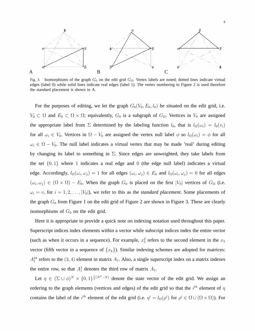
Fig. 3. Isomorphisms of the graphG0 on the edit gridGΩ. Vertex labels are noted; dotted lines indicate virtualedges (label 0) while solid lines indicate real edges (label 1). The vertex numbering in Figure 2 is used thereforethe standard placement is shown in A.

For the purposes of editing, we let the graphG0(V0, E0, l0) be situated on the edit grid, i.e.

V0 ⊂ Ω and E0 ⊂ Ω × Ω; equivalently,G0 is a subgraph ofGΩ. Vertices inV0 are assigned

the appropriate label fromΣ determined by the labeling functionl0, that is lΩ(ωi) = l0(vi)

for all ωi ∈ V0. Vertices inΩ − V0 are assigned the vertex null labelφ so lΩ(ωi) = φ for all

ωi ∈ Ω − V0. The null label indicates a virtual vertex that may be made ’real’ during editing

by changing its label to something inΣ. Since edges are unweighted, they take labels from

the set0, 1 where 1 indicates a real edge and0 (the edge null label) indicates a virtual

edge. Accordingly,lΩ(ωi, ωj) = 1 for all edges(ωi, ωj) ∈ E0 and lΩ(ωi, ωj) = 0 for all edges

(ωi, ωj) ∈ (Ω × Ω) − E0. When the graphG0 is placed on the first|V0| vertices ofGΩ (i.e.

ωi = vi for i = 1, 2, . . . , |V0|), we refer to this as thestandard placement. Some placements of

the graphG0 from Figure 1 on the edit grid of Figure 2 are shown in Figure 3. These are clearly

isomorphisms ofG0 on the edit grid.

Here it is appropriate to provide a quick note on indexing notation used throughout this paper.

Superscript indices index elements within a vector while subscript indices index the entire vector

(such as when it occurs in a sequence). For example,x25 refers to the second element in thex5

vector (fifth vector in a sequence ofxk). Similar indexing schemes are adopted for matrices:

A341 refers to the(3, 4) element in matrixA1. Also, a single superscript index on a matrix indexes

the entire row, so thatA31 denotes the third row of matrixA1.

Let η ∈ (Σ ∪ φ)N × 0, 1 12(N2−N) denote the state vector of the edit grid. We assign an

ordering to the graph elements (vertices and edges) of the edit grid so that theith element ofη

contains the label of theith element of the edit grid (i.e.ηi = lΩ(ρi) for ρi ∈ Ω∪ (Ω×Ω)). For

10

i ρi ηiA ηi

B ηiC πi

A πiB πi

C

1 ω1 α β φ 1 4 52 ω2 β φ φ 2 1 43 ω3 β β β 3 3 34 ω4 φ α β 4 5 25 ω5 φ φ α 5 2 16 (ω1, ω2) 1 0 0 6 8 157 (ω1, ω3) 1 1 0 7 13 148 (ω1, ω4) 0 1 0 8 15 129 (ω1, ω5) 0 0 0 9 11 910 (ω2, ω3) 1 0 0 10 7 1311 (ω2, ω4) 0 0 0 11 9 1112 (ω2, ω5) 0 0 0 12 6 813 (ω3, ω4) 0 1 1 13 14 1014 (ω3, ω5) 0 0 1 14 10 715 (ω4, ω5) 0 0 1 15 12 6

TABLE I

ELEMENT ORDERINGS, STATE VECTORS, AND CORRESPONDING STATE VECTOR PERMUTATIONS FOR THE

ISOMORPHISMS OFG0 ON THE EDIT GRID AS SHOWN INFIGURE 3. THE VECTOR OF EDIT GRID GRAPH

ELEMENTS IS DENOTED BYρ, THE STATE VECTORS ARE DENOTED BYηA, ηB , AND ηC , AND THE STATE

VECTOR PERMUTATIONS ARE DENOTED BYπA, πB , AND πC FOR THE CORRESPONDING ISOMORPHISM IN

FIGURE 3. NOTE THAT THE NUMBERING OF THE EDIT GRID VERTICESωi SHOWN IN FIGURE 2 IS USED.

example, the element orderings and state vectors for the graphs in Figure 3 are shown in Table

I.

We perform a finite sequence of graph edits to transform the graphG0(V0, E0, l0) situated on

the edit gridGΩ(Ω, Ω×Ω, lΩ) into the graphG1(V1, E1, l1) (such thatV1 ⊂ Ω andE1 ⊂ Ω×Ω).

Vertex edits consist of insertion, deletion, or relabeling to some other symbol inΣ. Edge edits

consist of insertion or deletion. Using the null labels introduced above, we may interpret all

graph edits as relabeling of real and virtual elements. For example, changing the label of a

virtual edge from0 to 1 corresponds to the insertion of that edge into the graphG(V, E, l).

Similarly, relabeling an edge from1 to 0 amounts to deleting that edge. Vertex insertion or

deletion is a bit more complex in that it also typically involves edge edits; however there is

a natural decomposition of the vertex edit that is consistent with this framework. Consider a

vertex deletion whereby a vertex is removed from the graph along with all edges adjacent to

that vertex. We may delete the vertex by changing its labelσ ∈ Σ to φ and relabeling all edges

11

adjacent to it from1 to 0. Vertex insertion may involve attaching the new vertex to the existing

graph via an edge. Again this process is easily decomposed by relabeling a virtual vertex from

φ to some desired labelσ ∈ Σ and changing the label of an appropriate virtual edge from0

to 1. Thus it suffices to consider the transforming of edge and vertex labels as the fundamental

operation for editing.

Edits essentially serve to alter the state of the edit grid. Thus we may specify a sequence of

edits by noting the sequence of edit grid state vectorsηkMk=0 resulting from these edits. Suppose

we wish to transform a graphG0 into a graphG1 by performing edit operations. Assume at this

point that the initial state of the edit gridη0 containsG0 in its standard placement. We must

have the final stateηM be such that it describesG1 situated in some fashion on the edit grid.

Thus if Γ1 is the set of state vectors corresponding to all isomorphisms ofG1 on the edit grid,

we must haveηM ∈ Γ1. Two different state sequences for transforming the exampleG0 into the

exampleG1 of Figure 1 are shown in Figure 4.

The set of all isomorphisms of a graphGn on the edit grid,Γn, may be defined in terms of the

standard placement ofGn denoted byηn andΠ–the set of all permutation mappings describing

isomorphisms of the edit gridGΩ–as in Eq. (1).

Γn =

η | ∃π ∈ Π s.t.ηi = ηπi

n

(1)

Note thatΠ does not contain all possible permutations of the elements of the state vectorη

because elements ofΠ must describe an isomorphism of the edit grid. For example, an edit grid

with two verticesΩ = ω1, ω2 has only two isomorphisms:ω′1 = ω1, ω′

2 = ω2 and ω′1 = ω2,

ω′2 = ω1. Assuming the graph elements are indexed asρ = (ω1, ω2, (ω1, ω2)), there are only two

permutations of the state vector that compriseΠ: π1 = (1, 2, 3) and π2 = (2, 1, 3). Indeed, it

will always be the case that|Π| = N !. The permutations of the state vector corresponding to

the isomorphisms ofG0 in Figure 3 are given in Table I.

We define a cost functionc : (Σ∪φ)2∪0, 12 → <+ that assigns a nonnegative cost to each

graph edit. The cost of an edit grid state transition denoted asC(ηk−1, ηk) is simply the sum of

12

η0 η1

η0 η1 η2

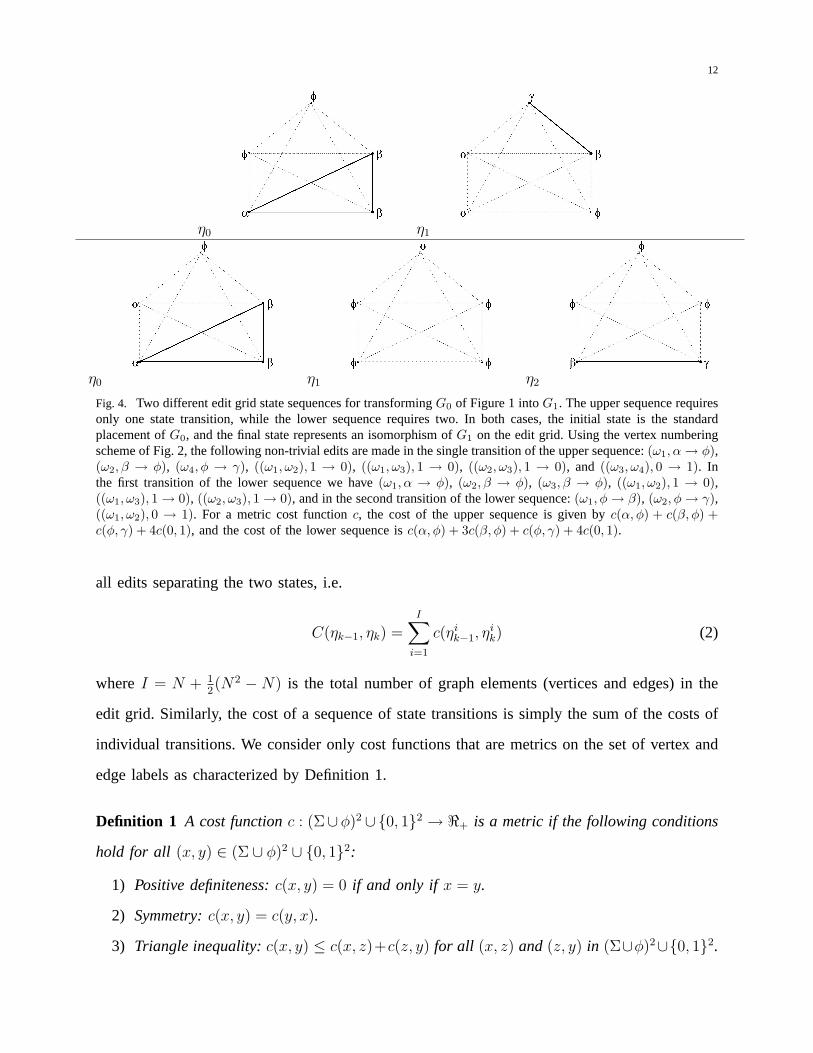
Fig. 4. Two different edit grid state sequences for transformingG0 of Figure 1 intoG1. The upper sequence requiresonly one state transition, while the lower sequence requires two. In both cases, the initial state is the standardplacement ofG0, and the final state represents an isomorphism ofG1 on the edit grid. Using the vertex numberingscheme of Fig. 2, the following non-trivial edits are made in the single transition of the upper sequence:(ω1, α → φ),(ω2, β → φ), (ω4, φ → γ), ((ω1, ω2), 1 → 0), ((ω1, ω3), 1 → 0), ((ω2, ω3), 1 → 0), and ((ω3, ω4), 0 → 1). Inthe first transition of the lower sequence we have(ω1, α → φ), (ω2, β → φ), (ω3, β → φ), ((ω1, ω2), 1 → 0),((ω1, ω3), 1 → 0), ((ω2, ω3), 1 → 0), and in the second transition of the lower sequence:(ω1, φ → β), (ω2, φ → γ),((ω1, ω2), 0 → 1). For a metric cost functionc, the cost of the upper sequence is given byc(α, φ) + c(β, φ) +c(φ, γ) + 4c(0, 1), and the cost of the lower sequence isc(α, φ) + 3c(β, φ) + c(φ, γ) + 4c(0, 1).

all edits separating the two states, i.e.

C(ηk−1, ηk) =I∑

i=1

c(ηik−1, η

ik) (2)

whereI = N + 12(N2 − N) is the total number of graph elements (vertices and edges) in the

edit grid. Similarly, the cost of a sequence of state transitions is simply the sum of the costs of

individual transitions. We consider only cost functions that are metrics on the set of vertex and

edge labels as characterized by Definition 1.

Definition 1 A cost functionc : (Σ∪φ)2 ∪0, 12 → <+ is a metric if the following conditions

hold for all (x, y) ∈ (Σ ∪ φ)2 ∪ 0, 12:

1) Positive definiteness:c(x, y) = 0 if and only if x = y.

2) Symmetry:c(x, y) = c(y, x).

3) Triangle inequality:c(x, y) ≤ c(x, z)+c(z, y) for all (x, z) and(z, y) in (Σ∪φ)2∪0, 12.

13

Assuming a metric cost function, the cost of the upper sequence in Figure 4 isc(α, φ)+c(β, φ)+

c(φ, γ) + 4c(0, 1), and the cost of the lower sequence isc(α, φ) + 3c(β, φ) + c(φ, γ) + 4c(0, 1).

With such a cost functionc, we have the following simple result.

Proposition 1 If c : (Σ∪ φ)2 ∪ 0, 12 → <+ is a metric on the set of labels thenC as defined

in Eq. (2) is a metric on the edit grid state space.

Proof: ExpandC in terms ofc using the definition in Eq. (2) and apply the metric properties

of c to trivially obtain the corresponding properties forC.

We thus have the following useful Lemma:

Lemma 1 Let c be a metric andηkMk=0 be a sequence of edit grid state vectors. Then for all

M ≥ 1, C(η0, ηM) ≤∑M

k=1 C(ηk−1, ηk).

Proof: TheM = 1 case is trivial and theM = 2 case follows from the triangle inequality.

Assume the claim holds for some valueM and proceed by induction:

C(η0, ηM+1) ≤ C(η0, ηM) + C(ηM , ηM+1)

≤∑M

k=1 C(ηk−1, ηk) + C(ηM , ηM+1)

=∑M+1

k=1 C(ηk−1, ηk)

(3)

where the first line in Eq. (3) follows from the triangle inequality and the second line uses the

induction hypothesis.

We now define the graph edit distance with respect to a cost functionc as

dc(G0, G1) = minηkM

k=1|ηM∈Γ1

M∑k=1

C(ηk−1, ηk) (4)

where η0 is the standard placement ofG0 on the edit grid,Γ1 is the set of state vectors

corresponding to isomorphisms ofG1 on the edit grid as in Eq. (1), andM is the maximum

number of allowed state transitions (this can be as large as desired, but we are only concerned

with finite graphs implyingM will be finite). There is no loss of generality by fixing the number

of terms in the summation of Eq. (4), since forM ′ < M transitions we can simply repeat the

final stateηM ′ so thatηk = ηM ′ for k = M ′ + 1, M ′ + 2, . . . M . Note that since there is a finite

14

number of state vector sequencesηkMk=1 such thatηM ∈ Γ1, the graph edit distance as defined

in Eq. (4) always exists. It essentially finds a state transition sequence of minimum cost that

transformsG0 into G1 (the minimizing sequence need not be unique). Since our cost function

is a metric, it seems logical that we should be able to achieve the minimum cost with only one

edit grid state transition. The following theorem shows this is indeed the case.

Theorem 1 For a given graph edit cost function,c : (Σ ∪ φ)2 ∪ 0, 12 → <+ that is a metric,

there exists a single state transition(η0, η1) such thatdc(G0, G1) = C(η0, η1) whereη0 is the

standard placement ofG0 and η1 ∈ Γ1.

Proof: Assume the initial stateη0 describesG0 in its standard placement on the edit grid,

and supposeηkMk=1 solves the graph edit minimization in Eq. (4)–this optimal sequence always

exists as argued earlier. Defineη1 = ηM , then we have

dc(G0, G1) = C(η0, η1) +∑M

k=2 C(ηk−1, ηk)

≥ C(η0, ηM)

= C(η0, η1)

(5)

where the second line follows from the first by applying Lemma 1. Now define the state sequence

ηkMk=1 so thatηk = η1 for all k. Then the positive definiteness of the metricC gives

C(η0, η1) = C(η0, η1) +∑M

k=2 C(ηk−1, ηk)

≥ minηkM

k=1|ηM∈Γ1

∑Mk=1 C(ηk−1, ηk)

= dc(G0, G1)

(6)

The second line follows becauseηM = η1 = ηM ∈ Γ1 and the proof is complete.

Theorem 1 allows the graph edit distance in Eq. (4) to be re-expressed equivalently as

dc(G0, G1) = minη1∈Γ1

C(η0, η1) = minπ∈Π

I∑i=1

c(ηi0, η

πi

1 ) (7)

where the second equality follows from the definition ofΓ1 in Eq. (1) andη0 and η1 are the

standard placements ofG0 andG1 respectively. Note that this one-state-transition result is crucial

for our binary linear programming formulation, and it hinges on the metric properties of the cost

15

function. Under a cost that is not a metric, there is no guarantee that the graph edit distance can

be computed with just one edit grid state transition. One might consider multiple state transitions

in a greedy algorithm for computing the graph edit distance in this case.

If π solves the minimization in Eq. (7), then we have

dc(G0, G1) =∑I

i=1 c(ηi0, η

πi

1 )

=∑

i|ρi∈V0∪V1∪E0∪E1c(ηi

0, ηπi

1 )(8)

Thus only elements of the edit grid comprising eitherG0 or G1 contribute to the sum; all other

elements have the null label in both states and therefore have zero cost. The most terms contribute

to the summation in Eq. (8) in the case whereV0 andV1 are disjoint. This suggests we need an

edit grid with no more thanN = |V0|+ |V1| vertices in order to compute the graph edit distance

in Eq. (7).

B. A Metric for Graphs

In addition to justifying the binary linear programming formulation to follow, Theorem 1 also

provides a simple means for showing that the graph edit distance (when derived from a metric

cost) is a metric itself on the set of undirected, unweighted graphs with vertex attributes (denoted

by Ξ). We need a preliminary lemma however. We have assumed for simplicity that the graph

edit minimization always starts with the graphG0 in its standard placement on the edit grid.

It seems that this should not be necessary; i.e. that the graph edit distance should be the same

regardless of whereG0 is on the edit grid. The following lemma establishes this.

Lemma 2 If η0 ∈ Γ0 whereΓ0 is as defined in Eq. (1), thendc(G0, G1) = minη1∈Γ1

C(η0, η1) =

minπ∈Π

∑Ii=1 c(ηi

0, ηπi

1 ).

Proof: Let ηi0 = ηπi

0 for the standard placementη0 then we have

dc(G0, G1) = minπ∈Π

∑Ii=1 c(ηi

0, ηπi

1 )

= minπ∈Π

∑Ij=1 c(ηπj

0 , ηππj

1 )

= minπ∈Π

∑Ij=1 c(ηj

0, ηπj

1 )

(9)

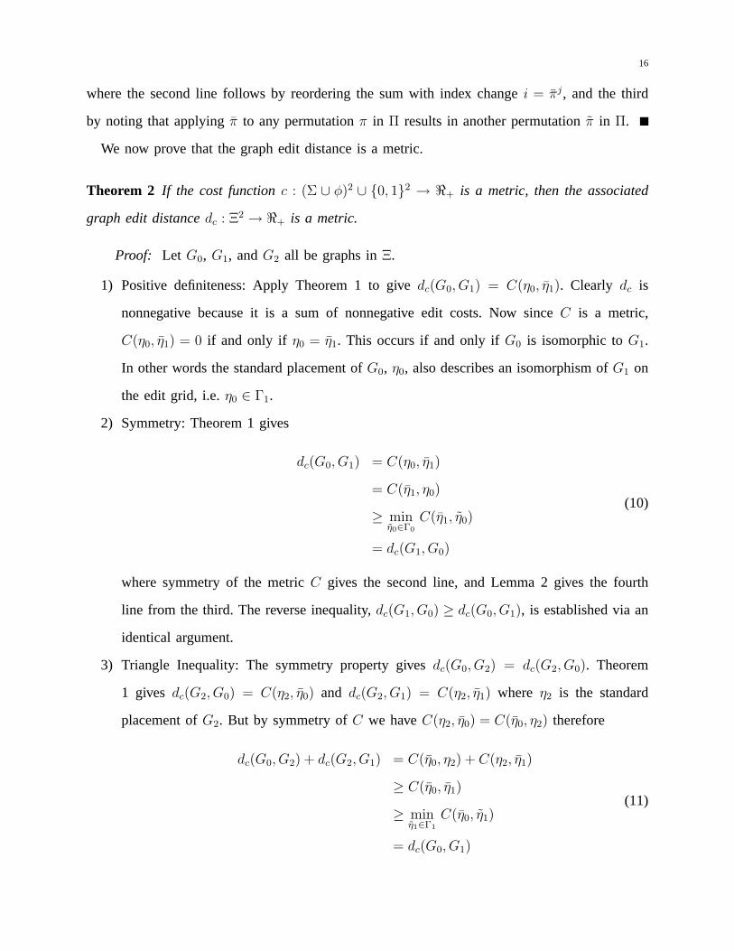
16

where the second line follows by reordering the sum with index changei = πj, and the third

by noting that applyingπ to any permutationπ in Π results in another permutationπ in Π.

We now prove that the graph edit distance is a metric.

Theorem 2 If the cost functionc : (Σ ∪ φ)2 ∪ 0, 12 → <+ is a metric, then the associated

graph edit distancedc : Ξ2 → <+ is a metric.

Proof: Let G0, G1, andG2 all be graphs inΞ.

1) Positive definiteness: Apply Theorem 1 to givedc(G0, G1) = C(η0, η1). Clearly dc is

nonnegative because it is a sum of nonnegative edit costs. Now sinceC is a metric,

C(η0, η1) = 0 if and only if η0 = η1. This occurs if and only ifG0 is isomorphic toG1.

In other words the standard placement ofG0, η0, also describes an isomorphism ofG1 on

the edit grid, i.e.η0 ∈ Γ1.

2) Symmetry: Theorem 1 gives

dc(G0, G1) = C(η0, η1)

= C(η1, η0)

≥ minη0∈Γ0

C(η1, η0)

= dc(G1, G0)

(10)

where symmetry of the metricC gives the second line, and Lemma 2 gives the fourth

line from the third. The reverse inequality,dc(G1, G0) ≥ dc(G0, G1), is established via an

identical argument.

3) Triangle Inequality: The symmetry property givesdc(G0, G2) = dc(G2, G0). Theorem

1 gives dc(G2, G0) = C(η2, η0) and dc(G2, G1) = C(η2, η1) where η2 is the standard

placement ofG2. But by symmetry ofC we haveC(η2, η0) = C(η0, η2) therefore

dc(G0, G2) + dc(G2, G1) = C(η0, η2) + C(η2, η1)

≥ C(η0, η1)

≥ minη1∈Γ1

C(η0, η1)

= dc(G0, G1)

(11)

17

where the second line follows from the triangle inequality forC, and Lemma 2 gives the

fourth line from the third.

C. Binary Linear Program for the Graph Edit Distance

In order to develop a binary linear program for computing the graph edit distance, we organize

the labels in the edit grid state vector using the adjacency matrix representation. The elements

of the adjacency matrix consist of edge labels, and we associate a vertex label with each

row(column) of the matrix (the matrix is symmetric since the graphs of interest are undirected).

We adopt the ordering scheme in Table I, so that ifAk ∈ 0, 1N×N is the adjacency matrix

corresponding to edit grid state vectorηk then the vertex labelηik is associated with theith

row(column) ofAk for i = 1, 2, . . . , N (i.e. l(Aik) = ηi

k), and the upper half of the matrix is

given by Aijk = η

iN+j− i2+i2

k for i < j ≤ N–the lower half follows similarly from symmetry.

All zeros lie on the diagonal ofAk. For example, the adjacency matrix representations of the

isomorphisms in Figure 3 (with state vectors in Table (I) are given by

AA =

0 1 1 0 0

1 0 1 0 0

1 1 0 0 0

0 0 0 0 0

0 0 0 0 0

α

β

β

φ

φ

AB =

0 0 1 1 0

0 0 0 0 0

1 0 0 1 0

1 0 1 0 0

0 0 0 0 0

β

φ

β

α

φ

AC =

0 0 0 0 0

0 0 0 0 0

0 0 0 1 1

0 0 1 0 1

0 0 1 1 0

φ

φ

β

β

α

(12)

where the vertex labels associated with each row/column are printed to the right of the corre-

sponding row.

The adjacency matrix representation also allows a convenient means for expressing an isomor-

phism permutationπ ∈ Π. We can represent the firstN elements ofπ as a permutation matrix

P ∈ 0, 1N×N–recall that the remaining12(N2−N) elements ofπ correspond to reordering of

the edges which is determined by the vertex permutation in the firstN elements. The elements of

the permutation matrixP corresponding toπ are given byP ij = δ(πi, j) for i, j = 1, 2, . . . , N

18

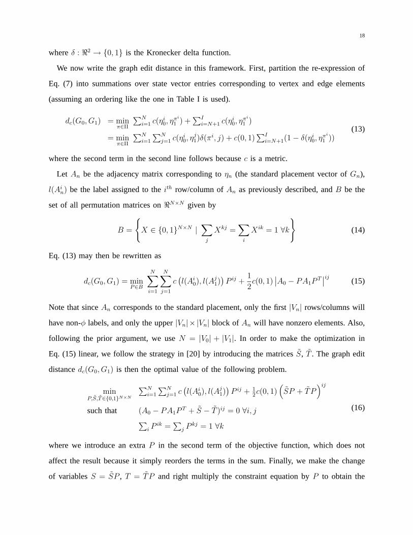
whereδ : <2 → 0, 1 is the Kronecker delta function.

We now write the graph edit distance in this framework. First, partition the re-expression of

Eq. (7) into summations over state vector entries corresponding to vertex and edge elements

(assuming an ordering like the one in Table I is used).

dc(G0, G1) = minπ∈Π

∑Ni=1 c(ηi

0, ηπi

1 ) +∑I

i=N+1 c(ηi0, η

πi

1 )

= minπ∈Π

∑Ni=1

∑Nj=1 c(ηi

0, ηj1)δ(π

i, j) + c(0, 1)∑I

i=N+1(1− δ(ηi0, η

πi

1 ))(13)

where the second term in the second line follows becausec is a metric.

Let An be the adjacency matrix corresponding toηn (the standard placement vector ofGn),

l(Ain) be the label assigned to theith row/column ofAn as previously described, andB be the

set of all permutation matrices on<N×N given by

B =

X ∈ 0, 1N×N |

∑j

Xkj =∑

i

X ik = 1 ∀k

(14)

Eq. (13) may then be rewritten as

dc(G0, G1) = minP∈B

N∑i=1

N∑j=1

c(l(Ai

0), l(Aj1))P ij +

1

2c(0, 1)

∣∣A0 − PA1PT∣∣ij (15)

Note that sinceAn corresponds to the standard placement, only the first|Vn| rows/columns will

have non-φ labels, and only the upper|Vn|× |Vn| block of An will have nonzero elements. Also,

following the prior argument, we useN = |V0| + |V1|. In order to make the optimization in

Eq. (15) linear, we follow the strategy in [20] by introducing the matricesS, T . The graph edit

distancedc(G0, G1) is then the optimal value of the following problem.

minP,S,T∈0,1N×N

∑Ni=1

∑Nj=1 c

(l(Ai

0), l(Aj1))P ij + 1

2c(0, 1)

(SP + TP

)ij

such that (A0 − PA1PT + S − T )ij = 0 ∀i, j∑

i Pik =

∑j P kj = 1 ∀k

(16)

where we introduce an extraP in the second term of the objective function, which does not

affect the result because it simply reorders the terms in the sum. Finally, we make the change

of variablesS = SP , T = TP and right multiply the constraint equation byP to obtain the

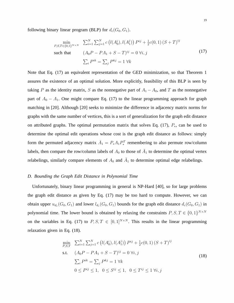
19

following binary linear program (BLP) fordc(G0, G1).

minP,S,T∈0,1N×N

∑Ni=1

∑Nj=1 c

(l(Ai

0), l(Aj1))P ij + 1

2c(0, 1) (S + T )ij

such that (A0P − PA1 + S − T )ij = 0 ∀i, j∑i P

ik =∑

j P kj = 1 ∀k

(17)

Note that Eq. (17) an equivalent representation of the GED minimization, so that Theorem 1

assures the existence of an optimal solution. More explicitly, feasibility of this BLP is seen by

takingP as the identity matrix,S as the nonnegative part ofA1−A0, andT as the nonnegative

part of A0 − A1. One might compare Eq. (17) to the linear programming approach for graph

matching in [20]. Although [20] seeks to minimize the difference in adjacency matrix norms for

graphs with the same number of vertices, this is a sort of generalization for the graph edit distance

on attributed graphs. The optimal permutation matrix that solves Eq. (17),P∗, can be used to

determine the optimal edit operations whose cost is the graph edit distance as follows: simply

form the permuted adjacency matrixA1 = P∗A1PT∗ remembering to also permute row/column

labels, then compare the row/column labels ofA0 to those ofA1 to determine the optimal vertex

relabelings, similarly compare elements ofA0 and A1 to determine optimal edge relabelings.

D. Bounding the Graph Edit Distance in Polynomial Time

Unfortunately, binary linear programming in general is NP-Hard [40], so for large problems

the graph edit distance as given by Eq. (17) may be too hard to compute. However, we can

obtain upperudc(G0, G1) and lowerldc(G0, G1) bounds for the graph edit distancedc(G0, G1) in

polynomial time. The lower bound is obtained by relaxing the constraintsP, S, T ∈ 0, 1N×N

on the variables in Eq. (17) toP, S, T ∈ [0, 1]N×N . This results in the linear programming

relaxation given in Eq. (18).

minP,S,T

∑Ni=1

∑Nj=1 c

(l(Ai

0), l(Aj1))P ij + 1

2c(0, 1) (S + T )ij

s.t. (A0P − PA1 + S − T )ij = 0 ∀i, j∑i P

ik =∑

j P kj = 1 ∀k

0 ≤ P ij ≤ 1, 0 ≤ Sij ≤ 1, 0 ≤ T ij ≤ 1 ∀i, j

(18)

20

For n variables, a linear program can be solved inO(n3.5) time using an interior point method

[43]. Thus the lower bound can be computed inO(N7) time since the linear program in Eq.

(18) hasO(N2) variables. If ldc(G0, G1) is the optimal value of Eq. (18) thenldc(G0, G1) ≤

dc(G0, G1) because the feasible region of the problem in Eq. (17) is a subset of the feasible

region of the problem in Eq. (18). It follows that Eq. (18) is always feasible because Eq. (17) is

always feasible as argued earlier. Thus the Weierstrass theorem assures existence of an optimal

value since we are minimizing a linear functional over a nonempty compact set [44]. Notice

that since the optimal matrixP∗ that solves Eq. (18) is only guaranteed to be doubly stochastic,

not necessarily a permutation matrix, there may not be a set of edit operations that achieves the

lower boundldc(G0, G1). However in the event thatP∗ is a permutation matrix, such a set can

be constructed as described in the previous section, and the optimal value of Eq. (18) is in fact

the graph edit distance.

The upper bound is obtained in polynomial time by solving the assignment problem with only

the vertex edit term. The assignment problem is given by

minP∈0,1N×N

∑Ni=1

∑Nj=1 c

(l(Ai

0), l(Aj1))P ij

such that∑

i Pik =

∑j P kj = 1 ∀k

(19)

Note that the optimal value of Eq. (19) always exists since there is a finite number of permutations

and the identity always serves as a feasible permutation. Indeed, the Hungarian method may be

used to solve it inO(N3) time [40]. If P∗ is an optimal solution of Eq. (19), we computeS∗

as the nonnegative part ofP∗A1−A0P∗ andT∗ as the nonnegative part ofA0P∗−P∗A1 so that

(P∗, S∗, T∗) is in the feasible region of the problem in Eq. (17).udc(G0, G1) is then computed

by evaluating the objective function in Eq. (17) at(P∗, S∗, T∗). It follows that dc(G0, G1) ≤

udc(G0, G1). SinceP∗ is a permutation matrix for the solution to Eq. (19), a set of edit operations

whose cost is the upper bound to the graph edit distance can always be determined.

E. Selecting a Cost Metric for Uniform Distribution

We have assumed that the cost metric that characterizes the graph edit distance is available,

however, in a given application it may not be clear what is the ’best’ cost metric to use. We

21

propose an empirical method for selecting a metric based on prior information suitable for a

recognition problem. Suppose there is a set of prototype graphsGiNi=1, and we classify a sample

graphG0 by selecting the prototype that is closest to it with respect to a graph distance metric.

Prior information might suggest that the prototypes should be roughly uniformly distributed in

the metric space of graphs defined by the graph edit distance. We can then choose an optimal

metric with respect to this objective. Such a criterion will also have the effect of minimizing

the worst case classification error, since it equalizes the probability of error under the minimum

distance classifier.

Note that for a set of points uniformly distributed in some space, all nearest neighbor distances

are the same. To uniformly distribute the prototypes, we first determine all pairwise distances

using a cost metric that assigns unity to all edits, i.e.c(0, 1) = 1, c(l(Ai

0), l(Aj1))

= 0 if

l(Ai0) = l(Aj

1) and c(l(Ai

0), l(Aj1))

= 1 otherwise. The resulting edit operations under the unit

cost matching are then fixed, and we optimize the normalized variance of pairwise distances

over the set of cost metrics.

To carry out this optimization, we must tabulate the edits necessary to match each graph

with its q nearest neighbors under a unit cost function. If the graphs are not too large, we may

compute a permutation matrix that actually solves the graph edit distance minimization in Eq.

(17). If this is not the case a permutation matrix that solves the assignment problem in Eq. (19)

with unit weights will serve as a reasonable approximation. We consider each nearest neighbor

pair only once. For example ifGi hasGj as one of itsq nearest neighbors andGj hasGi as one

of its q nearest neighbors, then the edits necessary to matchGi to Gj are tabulated only once.

After determining the unit cost matching between all prototype pairs, we order all distinct

edits that occur in any prototype matching and tabulate the vectorsHjKj=1. H i

j indicates the

number of times theith edit occurs to match thejth pair of nearest neighbor prototypes (under

a unit cost function) andK is the number of distinct nearest neighbor pairs. Ifc is a vector

containing the corresponding edit costs, then the graph edit distance between thejth pair is given

by dc(Gj0, Gj1) = HTj c. For example, consider as prototypes the standard placements ofG0 and

G1 as shown in the lower left and lower right respectively of Figure 4. If we order the edits as

22

(α, β, α, γ, α, φ, β, γ, β, φ, γ, φ, 1, 0) then the vector of countsH corresponding

to this matching is(1, 0, 0, 1, 1, 0, 2). Indeed, the dimension of eachHj vector will always be

12(|Σ|2 + |Σ|) + 1 for a vertex label setΣ and edge label set0, 1.

Using this notation, the scaled variance of pairwise distances is then given by

Kσ2d = cT

K∑i=1

(Hi −

1

K

K∑j=1

Hj

)(Hi −

1

K

K∑j=1

Hj

)T c ≡ cT Qc (20)

We also require the cost function to be a metric. Positive definiteness may be enforced by

selecting some minimum positive cost for all editsa > 0. Symmetry is enforced implicitly by

binning symmetric edits together in the count vectorH and assigning the same cost to both

edits. Finally, we must include linear inequalities of the formci + cj − ck ≥ 0 to assure the

triangle inequality holds for all sets of three vertex labels. There are12|Σ|(|Σ|2− 1) of these; we

define the matrixF such thatFc ≥ 0 summarizes the triangle inequalities. The variance should

be normalized before optimizing so that the result does not depend on the scale of the costs

(determined bya). If we normalize by the sum of the costs, a convex program results where any

local optimum is also a global optimum [45]. The optimal costs are then given by the convex

program:

minc

cT QceT c

s.t. Fc ≥ 0

ci ≥ a ∀i

(21)

wheree is a vector of ones. Note that the problem is always feasible because if we takeci = a

for all i, then all necessary triangle inequalities are satisfied. Furthermore, the choice ofa is

irrelevant, provideda > 0; we only need that the costsci (all of which correspond to nontrivial

edits) be uniformly bounded below away from zero so that a metric results. For any givena

we may choosea′ = κa for someκ > 0, and the change of variablesc′ = κc results in the

original optimization problem in Eq. (21). The following proposition establishes the convexity

of the problem. A barrier method will solve the convex program in polynomial time [45].

Proposition 2 The optimization problem in Eq. (21) is convex.

23

Proof: All inequalities are linear, so we need only show that the objective function is

convex. The objective function is defined over the positive orthant, which is a convex set, so

the function is convex if and only if its Hessian is positive semidefinite [45]. LetΨ(c) = cT QceT c

be the objective function of the problem. The Hessian quadratic form with an arbitrary vectorv

may be factored as

vT (∇2Ψ(c))v = vT(

2(eT c)3

[(cT Qc)eeT + (eT c)2Q− (eT c)(ecT Q + QceT )

])v

= 2(eT c)3

∥∥∥(eT v)Q12 c− (eT c)Q

12 v∥∥∥2

≥ 0(22)

where Q12 is the matrix square root ofQ which exists becauseQ as defined in Eq. (20) is

obviously symmetric positive semidefinite. The inequality follows becausec is defined over the

positive orthant so(eT c)3 > 0; thus∇2Ψ(c) 0.

III. C HEMICAL GRAPH RECOGNITION

As an application, we use the graph edit distance to recognize chemical graphs in the context

of a chemical information system. We selected our database of 135 similar molecules from

the Klotho Biochemical Compounds Declarative Database, which consists of small molecules

useful in describing mechanisms of biochemical reactions [42]. Only molecules with 18 or fewer

atoms were used so that we could compute exact distance measures in reasonable time. Attributed

undirected graphs were generated from the 135 molecules (referred to aschemical graphs), then

the optimal edit costs were computed to uniformly distribute them in the graph metric space.

Finally, we compared the recognition ability of the graph edit distance with optimal costs and

unit costs to that of two maximum common subgraph based distance metrics by using randomly

perturbed prototype graphs from the database.

We first generated chemical graphs from the molecular structure diagrams by associating

atoms with vertices and bonds with edges. Each vertex was labeled by the chemical symbol

of the element to which that vertex corresponded. Our vertex label alphabet was thus given by

Σ = H, C,O, N,Cl, P, S, Br, Si. Vertices in the graph were connected by an edge if and

only if their corresponding atoms were bonded (single bonds, double bonds, etc. were treated

equally). For example, the chemical graphs derived from the molecules adenine, thymine, and

24

A B C

Fig. 5. Chemical graphs derived from the familiar molecules from DNA: adenine (A), thymine (B), and cytosine(C).

cytosine are shown in Figure 5.

In order to compute the optimal edit costs, we treated all 135 molecules as nearest neighbors

(so that the number of nearest neighbor pairsK is given by 12(1352 − 135) = 9045). Indeed,

all molecules in the database are of similar structure and function. In the context of a larger

chemical database consisting of thousands or millions of molecules, one might suppose our 135

molecules are the result of some clustering [46] or pre-screening procedure [7] performed using

a quickly computed similarity measure in order to isolate only the most likely matches to a given

input. For example, one might use the lower bound obtained by the LP relaxation in Eq. (18)

as a pre-screening criterion. We then wish to homogenize the most likely matches with respect

to the graph edit distance using the optimal edit costs.

We used the permutation matrices that solve the binary linear program in Eq. (17) with unit

costs to tabulate the edit operation counts in the vectorsHj necessary for optimizing the cost

metric. The publicly availablelp solve program was used to solve the integer program; it

implements the simplex method in a branch-and-bound algorithm [47]. The optimal edit costs

were then computed by solving the convex program in Eq. (21) witha = 0.1 using a barrier

method. The optimal edit costs for vertex relabelings are shown in Figure 6–the optimal edge

edit cost was computed to bec(0, 1) = 0.1. The associated edit counts tabulated over all pairs

in the database matched with unity cost function are shown in Figure 7. The most frequently

inserted/deleted atom types in matching the prototypes wereH, C, and O, while the most

frequent relabelings wereO ↔ H andO ↔ N . Note that there is roughly an inverse relationship

between the number of times a particular edit occurs and its optimal cost, as one might expect.

25

Fig. 6. Optimal edit costs resulting from the convex program in Eq. (21). There is a label associated with eachgroup of bars. Within the group, the edit cost of changing the group label to an individual label corresponds to theheight of the bar below that individual label. The optimal edge edit costc(0, 1) was0.1.

This does not hold exactly, however, because the edit costs must also satisfy the necessary

triangle inequalities.

The maximum common subgraph (MCS) is frequently used as a similarity measure for

chemical graphs [8]. Also, some graph metrics have been devised based on the MCS that are

appropriate for comparison to our graph edit based metric [13], [11], [12]. There are some

variations in the literature on what is meant by ’maximum common subgraph.’ The differences

amount to whether the vertices or the edges are the defining feature of the subgraph, resulting

in a ’maximum common induced subgraph (MCIS)’ or a ’maximum common edge subgraph

(MCES)’ respectively [9]. The MCIS is used in [48], while the MCES is used in [49], [50]. We

will use the MCIS, which satisfies the MCS definition given in [24]. A slightly modified version

of the distance metric proposed in [13] appropriate for the MCIS is given by

dmcs1(G0, G1) = |V0|+ |V1| − 2|V01| (23)

whereG01(V01, E01, l01) is the MCS (MCIS) of graphsG0(V0, E0, l0) and G1(V1, E1, l1). Note

that we are being somewhat careless with language–although we say ’the’ MCS, it need not be

26

Fig. 7. Total number of occurrences of each type of vertex edit tabulated over all pairs of database graphs matchedwith unit cost function. There is a label associated with each group of bars. Within the group, the edit cost ofchanging the group label to an individual label corresponds to the height of the bar below that individual label.We see thatH, C, andO are the most frequently inserted/deleted atom types, and the most frequent relabelingsareO ↔ H andO ↔ N . Note that edits occurring more frequently are typically assigned a lower cost (Figure 6).There were 60974 total edge edits (not shown).

unique. In addition to the MCS metric of Eq. (23), we also compared recognition performance

to the following metric that is proposed in [11].

dmcs2(G0, G1) = 1− |V01|max(|V0|, |V1|)

(24)

It has been shown that computing the MCS of graphsG0(V0, E0, l0) and G1(V1, E1, l1) is

equivalent to computing the maximum clique in a modular product graphGp(Vp, Ep) [51]. In

general finding the maximum clique is NP-Hard, so the worst case complexity is equivalent to

binary linear programming [10]. The modular product graph is defined by the sets

Vp = (v0, v1) | v0 ∈ V0, v1 ∈ V1, l0(v0) = l1(v1)

E+ = [(v0, v1), (u0, u1)] | v0 6= u0, v1 6= u1, (v0, u0) ∈ E0, (v1, u1) ∈ E1

E− = [(v0, v1), (u0, u1)] | v0 6= u0, v1 6= u1, (v0, u0) /∈ E0, (v1, u1) /∈ E1

Ep = E+ ∪ E−

(25)

We computed the MCS by using the algorithm in [52] to find the maximum clique in the modular

27

A B

C D

Fig. 8. Pairwise distance histograms between all 9045 pairs of 135 prototype graphs in the database. Distancescomputed with the GEDo are shown in A, those computed with the GEDu are in B, those computed with the MCS1metric are shown in C, and those computed with the MCS2 metric are in D. Ideally, all pairwise distances wouldbe the same. Since the GEDo distances are more concentrated, the GEDo more uniformly distributes the prototypegraphs. This should result in less ambiguity in the graph recognition phase, whereby the distance between a samplegraph and each prototype graph is computed.

product graph.

We calculated all 9045 pairwise distances between prototype graphs in the database using both

the graph edit distance with optimal costs (GEDo) in Figure 6 and unit costs (GEDu), along

with the two MCS distance metrics (MCS1 and MCS2) given in Eqs. (23) and (24) respectively.

Histograms of the resulting pairwise distances are shown in Figure 8. Note that the GEDo

pairwise distances are more concentrated around a single value than either of the MCS distances

or the GEDu; this indicates the GEDo more uniformly distributes the prototypes in the graph

metric space.

The ability of the four metrics to recognize input graphs as one of the prototype graphs in

the database was tested next. An error-correcting graph isomorphism is indeed appropriate here,

since each input graph was generated by applying a predetermined number of editsM (where

M ∈ 1, 2, 3, 4, 5, 6) to a randomly chosen prototype graph. The edits applied fell into one of

the following five categories:

1) edge edit: M edges edits are selected with insertion and deletion having equal probability.

28

Once theM edit operations are selected, pairs of vertices between which edges should be

either inserted or deleted are selected at random.

2) vertex deletion: M vertices are selected to be deleted. First a label to be deleted is chosen

with deletion probabilities given by normalizing the edit counts over theφ-group in Figure

7. Among the vertices having the chosen label, one is selected at random to be deleted

along with all edges connected to it.

3) vertex insertion: M vertices are inserted. First a label to be inserted is chosen with insertion

probabilities given by normalizing the edit counts over theφ-group in Figure 7. A vertex

with the chosen label is then connected by a single edge to an existing vertex in the graph

chosen at random.

4) vertex relabeling: M vertices are selected to be relabeled. First a pair of labels is chosen

with probabilities given by normalizing the edit counts in Figure 7 over all non-φ edits.

Among the vertices having a label that matches one in the pair, one is selected at random

and its label is changed to the complementary label in the pair.

5) random: TheM edits to be performed are randomly chosen from the above four categories

with each having equal probability.

Note that in performing vertex edits, we used the edit counts in Figure 7 as a guide so that

the edits made would represent likely errors, say, in transcribing the chemical formula of one of

the prototype graphs. Also, no regard was given to physical laws governing bonding, therefore

some input graphs may not be physically realizable molecules. Examples of the different edit

types applied to the adenine molecule are shown in Figure 9.

For each of the five edit categories, we generated ten input graphs from randomly chosen

prototype graphs for each value ofM (number of edits) ranging from 1 to 6; this resulted in

6 × 10 × 5 = 300 sample input graphs. We then attempted to recognize the input graph by

computing the distance (using GEDo, GEDu, MCS1, and MCS2) between the input graph and

each of the 135 prototypes. There were300× 135 = 40, 500 distinct input graph/prototype pairs

matched using each of the four metrics to determine the corresponding graph distances. Due

to the large number of matchings considered and the exponential complexity of the algorithms

29

A B

C D

Fig. 9. Example edits applied to the adenine chemical graph shown in Figure 5A. Two edge edits (one insertion,one deletion) are shown in A with the thick dashed line representing the inserted edge and the thin dashed line isthe deleted edge. Two vertex deletions (represented by dotted lines and open boxes) are shown in B. C shows twovertex insertions (underlined), and D shows two vertex relabelings (underlined).

tested, we allowed a maximum of 45 seconds for any distance computation. If an optimal solution

was not found within the allotted time, the best feasible suboptimal solution available was used.

Running on Pentium 4, 2GHz processors, the average time required to solve the binary linear

program necessary for GEDo or GEDu withlp solve [47] was about 1.3 seconds, while the

average time required to compute the maximum common subgraph using the maximum clique

algorithm of [52] was about 0.1 seconds. Although the MCS routine is about ten times faster

here, these times will vary depending on the particular algorithm/implementation one chooses

for binary linear programming and maximum common subgraph detection.

We say an input graph is correctly recognized if it is closest (with respect to the appropriate

distance metric) to the prototype graph from which it was generated. A ’classifier ratio’ (CR)

as given in Eq. (26) was computed for each input graph in order to gauge the level of ambiguity

associated with the classification.

CR =d∗do

(26)

Whered∗ is the graph edit distance between the sample graph and the prototype from which it

was generated, anddo is the distance between the sample and the nearest incorrect prototype

30

Metric 1) Edge Edit 2) Vertex Delete 3) Vertex Insert 4) Vertex Relabel 5) RandomGEDo 1.00 , 0.65 0.33 , 0.79 0.65 , 0.71 0.88 , 0.71 0.75 , 0.76GEDu 0.98 , 0.70 0.25 , 0.85 0.45 , 0.87 0.95 , 0.69 0.65 , 0.80MCS1 0.67 , 0.83 0.75 , 0.81 0.97 , 0.72 0.63 , 0.87 0.67 , 0.79MCS2 0.78 , 0.77 0.52 , 0.89 0.55 , 0.87 0.73 , 0.82 0.68 , 0.85

TABLE II

PROPORTION OF GRAPHS CORRECTLY RECOGNIZED AND AVERAGE CLASSIFIER RATIO FOR EACH EDIT TYPE

CATEGORY AVERAGED OVER ALL GRAPHS IN THAT CATEGORY. THESE ARE COMPUTED BY MARGINALIZING

THE PLOTS INFIGURE 10 OVER THE HORIZONTAL AXIS (NUMBER OF EDITS, M). THE FIRST NUMBER IN EACH

PAIR IS THE PROPORTION CORRECTLY RECOGNIZED AND THE SECOND NUMBER IS THE AVERAGE CLASSIFIER

RATIO (PC, CR). THE GED METRICS PERFORM BETTER IN THE CASE OF EDGE EDITS, VERTEX RELABELINGS,AND RANDOM EDITS (1, 4, AND 5); INDEED, THE GEDO METRIC CORRECTLY RECOGNIZES AT LEAST75% OF

GRAPHS IN THESE CATEGORIES. ONLY THE MCS1 METRIC PERFORMS WELL IN THE CASE OF VERTEX

DELETIONS AND INSERTIONS(2 AND 3) WITH AT LEAST 75% CORRECT RECOGNITION IN BOTH CASES. THE

GEDO METRIC (GED WITH OPTIMAL COSTS) HAS THE LOWEST AVERAGECR IN ALL CATEGORIES BUT ONE,INDICATING REDUCED CLASSIFICATION AMBIGUITY.

(’incorrect’ in that the sample was not generated from this prototype). The lowerCR is the less

ambiguous the classification.

The proportion of graphs correctly recognized by each metric along with average classifier

ratio associated with that metric for the five edit categories are shown in Figure 10. The classifier

ratios were averaged only over those graphs that were correctly classified. The marginal values

associated with these distributions averaged over the number of editsM are given in Table II.

Note that the GED metrics had superior performance in the edge edit, vertex relabeling, and

random edit categories; the GEDo metric correctly recognizes at least 75% of graphs in these

categories. The GED metrics were particularly successful in the edge edit category with all

graphs correctly recognized by the GEDo metric, which also gave a consistently lower classifier

ratio. The MCS1 metric was most robust in the case of vertex deletions and insertions (having

at least 75% correct recognition); indeed both GED metrics had significant trouble when three

or more vertices are deleted and trail off similarly in the case of vertex insertions. Undoubtedly,

the changes on the prototype graph caused by inserting/deleting three or more vertices were

so drastic that a different prototype was actually closer with respect to the GED to the sample

graph produced. The GED metrics remained strong for up to five vertex relabelings, however,

while the proportion correct for either MCS metric in this case decreased after three. In Table

31

1PC 2PC 3PC

1CR 2CR 3CR

4PC 5PC

4CR 5CR

Fig. 10. Proportion of graphs correctly recognized (PC) and average classifier ratios (CR) for the five differentedit categories: 1) edge edit, 2) vertex deletion, 3) vertex insertion, 4) vertex relabeling, and 5) random. Withineach plot, the letter above a bar denotes the metric used: A) GEDo (graph edit distance with optimal costs), B)GEDu (graph edit distance with unit costs), C) MCS1 (max common subgraph metric of Eq. (23)), and D) MCS2(max common subgraph metric of Eq. (24)). Each set of four bars corresponds to a different number of editsM ,indicated along the horizontal axis. Typically, as the number of edits increases, the proportion correctly recognizeddrops while the ambiguity of classification (as measured by the CR) rises. Note that the GED metrics performbetter in the case of edge edits, vertex relabelings, and random edits (1, 4, and 5). The MCS metrics perform betterin the case of vertex deletions and insertions (2 and 3). Marginal values of these distributions (averaged overM )are given in Table II.

32

II, we see that the optimal costs were indeed effective in reducing classification ambiguity as

measured by the CR since the GEDo metric has the lowest average CR in all categories but one.

IV. CONCLUSION

This paper develops a linear formulation of the graph edit distance for attributed graphs. We

prove that the derived GED is a metric and show how to compute it using a binary linear program.

Upper and lower bounds for the GED that can be computed in polynomial time are also given.

A chemical graph recognition problem is presented as an application of the graph matching

formalism. The edit costs are chosen using a normalized minimum variance criterion based on

the prior information that the database graphs should be uniformly distributed in the graph metric

space defined by the GED. This method is shown to give a metric that more uniformly distributes

a database of 135 chemical graphs with similar structure than comparable maximum common

subgraph based metrics. In recognizing chemical graphs generated by perturbing graphs in the

database, the GED metrics with optimal costs and unit costs are shown to correctly recognize

which prototype was perturbed more often than the MCS metrics in the case of edge edits and

vertex relabelings. The MCS metrics perform better in the case of vertex insertions and deletions.

When random edits are applied, the GED metrics are generally the best. Also, the GED with

optimized edit costs is shown to have its intended effect of reducing the level of ambiguity

associated with the chemical graph recognitions.

Unfortunately, the complexity of binary linear programming makes computing the GED be-

tween large graphs difficult using this method. However, the polynomial-time upper and lower

bounds may be readily employed in this case. Also, these could be used in pre-screening on

large chemical databases. For example, pre-screening may be done by rejecting all molecules

whose LP lower bound to the query exceeds a given value. Although we have developed a

metric for unweighted graphs, it can be directly extended to graphs with edge weights provided

the cost of editing these edges is proportional to the absolute difference in the weights with

positive proportionality constantk. Indeed, one could proceed from Eq. (17) with weighted

adjacency matricesA0, A1 used instead andc(0, 1) replaced byk. However, Eq. (17) would

become a mixed integer program since, depending on the weights,S andT may not be binary

33

matrices. Incorporating edge weights would yield a method applicable to 3-D structure searching

of chemical graphs where weights are assigned to the graph edges based on the length of the

bond they represent [6], along with other applications of weighted graphs. We anticipate the

results of this paper are applicable in any setting where it is necessary to compare graphical

models.

ACKNOWLEDGEMENTS

This work was partially supported by a Dept. of EECS Graduate Fellowship to the first author

and by the National Science Foundation under ITR contract CCR-0325571.

REFERENCES

[1] T. Pavlidis,Structural Pattern Recognition. New York: Springer-Verlag, 1977.

[2] L. Jianzhuang and L. Tsui, “Graph-based method for face identification from a single 2d line drawing,”IEEE Transactions

on Pattern Analysis and Machine Intelligence, vol. 23, no. 10, pp. 1106–1119, 2000.

[3] J. Llados, E. Marti, and J. Villanueva, “Symbol recognition by error-tolerant subgraph matching between region adjacency

graphs,”IEEE Transactions on Pattern Analysis and Machine Intelligence, vol. 23, no. 10, pp. 1137–1143, 2001.

[4] D. Shasha, J. Wang, and R. Giugno, “Algorithmics and applications of tree and graph searching,” inProc. 21st ACM

SIGMOD-SIGACT-SIGART, Madison, WI, June 2005.

[5] M. Johnson and G. Maggiora, Eds.,Concepts and Applications of Molecular Similarity. New York: John Wiley and Sons,

1990.

[6] G. Downs and P. Willett, “Similarity searching in databases of chemical structures,” inReviews in Computational Chemistry,

Vol. 7, K. Lipkowitz and D. Boyd, Eds. New York: VCH Publishers, Inc., 1996, pp. 1–66.

[7] J. Raymond and P. Willett, “Effectiveness of graph-based and fingerprint-based similarity measures for virtual screening

of 2d chemical structure databases,”J. Computer-Aided Molecular Design, vol. 16, pp. 59–71, 2002.

[8] P. Willett, “Matching of chemical and biological structures using subgraph and maximal common subgraph isomorphism

algorithms,” IMA Vol. Math. Appl., vol. 108, pp. 11–38, 1999.

[9] J. Raymond and P. Willett, “Maximum common subgraph isomorphism algorithms for the matching of chemical structures,”

J. Computer-Aided Molecular Design, vol. 16, pp. 521–533, 2002.

[10] M. Garey and D. Johnson,Computers and Intractability: A Guide to the Theory of NP-Completeness. San Francisco,

CA: W.H. Freeman, 1979.

[11] H. Bunke and K. Shearer, “A graph distance metric based on the maximal common subgraph,”Pattern Recognition Letters,

vol. 19, pp. 255–259, 1998.

[12] W. Wallis, P. Shoubridge, M. Kraetz, and D. Ray, “Graph distances using graph union,”Pattern Recognition Letters, vol. 22,

pp. 701–704, 2001.

34

[13] M. Johnson, M. Naim, V. Nicholson, and C. Tsai, “Unique mathematical features of the substructure metric approach to

quantitative molecular similarity analysis,” inGraph Theory and Topology in Chemistry, R. King and D. Rouvray, Eds.,

Mar. 1987, pp. 219–225.

[14] M.-L. Fernandez and G. Valiente, “A graph distance metric combining maximum common subgraph and minimum common

supergraph,”Pattern Recognition Letters, vol. 22, pp. 753–758, 2001.

[15] A. Torsello, D. Hidovic-Rowe, and M. Pelillo, “Polynomial-time metrics for attributed trees,”IEEE Transactions on Pattern

Analysis and Machine Intelligence, vol. 27, no. 7, pp. 1087–1099, July 2005.

[16] M. Gori, M. Maggini, and L. Sarti, “Exact and approximate graph matching using random walks,”IEEE Transactions on

Pattern Analysis and Machine Intelligence, vol. 27, no. 7, pp. 1100–1111, July 2005.

[17] B. McKay, “Practical graph isomorphism,”Congressus Numerantium, vol. 30, pp. 45–87, 1981.

[18] L. Cordella, P. Foggia, C. Sansone, and M. Vento, “A (sub)graph isomorphism algorithm for matching large graphs,”IEEE

Transactions on Pattern Analysis and Machine Intelligence, vol. 26, no. 10, pp. 1367–1372, Oct. 2004.

[19] W. Tsai and K. Fu, “Error-correcting isomorphisms of attributed relational graphs for pattern recognition,”IEEE

Transactions on Systems, Man, and Cybernetics, vol. 9, pp. 757–768, 1979.

[20] H. Almohamad and S. Duffuaa, “A linear programming approach for the weighted graph matching problem,”IEEE

Transactions on Pattern Analysis and Machine Intelligence, vol. 15, no. 5, pp. 522–525, May 1993.

[21] S. Umeyama, “An eigendecomposition approach to weighted graph matching problems,”IEEE Transactions on Pattern

Analysis and Machine Intelligence, vol. 10, no. 5, pp. 695–703, Sept. 1988.

[22] S. Gold and A. Rangarajan, “A graduated assignment algorithm for graph matching,”IEEE Transactions on Pattern Analysis

and Machine Intelligence, vol. 18, no. 4, pp. 377–387, Apr. 1996.

[23] B. van Wyk and M. van Wyk, “A pocs-based graph matching algorithm,”IEEE Transactions on Pattern Analysis and

Machine Intelligence, vol. 26, no. 11, pp. 1526–1530, Nov. 2004.

[24] H. Bunke, “Error correcting graph matching: on the influence of the underlying cost function,”IEEE Transactions on

Pattern Analysis and Machine Intelligence, vol. 21, no. 9, pp. 917–922, Sept. 1999.

[25] ——, “Recent developments in graph matching,”Proc. 15th Intl. Conf. on Pattern Recognition, vol. 2, pp. 117–124, Sept.

2000.

[26] R. Wagner and M. Fischer, “The string-to-string correction problem,”Journal of the Association for Computing Machinery,

vol. 21, no. 1, pp. 168–173, 1974.

[27] A. Hlaoui and S. Wang, “A new algorithm for inexact graph matching,”Proc. 16th Intl. Conf. on Pattern Recognition,

vol. 4, pp. 180–183, 2002.

[28] B. Messmer and H. Bunke, “Error-correcting graph isomorphism using decision trees,”Int. Journal of Pattern Recognition

and Art. Intelligence, vol. 12, pp. 721–742, 1998.

[29] R. Myers, R. Wilson, and E. Hancock, “Bayesian graph edit distance,”IEEE Transactions on Pattern Analysis and Machine

Intelligence, vol. 22, no. 6, pp. 628–635, June 2000.

[30] A. Robles-Kelly and E. Hancock, “Graph edit distance from spectral seriation,”IEEE Transactions on Pattern Analysis

and Machine Intelligence, vol. 27, no. 3, pp. 365–378, Mar. 2005.

35

[31] P. Bergamini, L. Cinque, A. Cross, and E. Hancock, “Efficient alignment and correspondence using edit distance,”

SSPR/SPR, pp. 246–255, 2000.

[32] K. Zhang, “A constrained edit distance between unordered labeled trees,”Algorithmica, vol. 15, no. 6, pp. 205–222, 1996.

[33] Z. Wang and K. Zhang, “Alignment between two rna structures,”MFCS, pp. 690–702, 2001.

[34] P. Klein, S. Tirthapura, D. Sharvit, and B. Kimia, “A tree-edit distance algorithm for comparing simple, closed shapes,”

Proc. ACM-SIAM Symp. Disc. Algorithms, pp. 696–704, 2000.

[35] M. Pavel,Fundamentals of Pattern Recognition. New York: Marcel Dekker, 1989.

[36] M. Neuhaus and H. Bunke, “A probabilistic approach to learning costs for graph edit distance,”Proc. 17th Intl. Conf. on

Pattern Recognition, vol. 3, pp. 389–393, 2004.

[37] T. Sebastian, P. Klein, and B. Kimia, “Recognition of shapes by editing their shock graphs,”IEEE Transactions on Pattern

Analysis and Machine Intelligence, vol. 26, no. 5, pp. 550–571, May 2004.

[38] G. Harper, G. Bravi, S. Pickett, J. Hussain, and D. Green, “The reduced graph descriptor in virtual screening and data-driven

clustering of high-throughput screening data,”J. Chem. Inf. Comput. Sci., vol. 44, pp. 2145–2156, 2004.

[39] P. Willett and V. Winterman, “A comparison of some measures for the determination of inter-molecular stuctural similarity,”

Quant. Struct.-Act. Relat., vol. 5, 1986.

[40] C. Papadimitriou and K. Steiglitz,Combinatorial Optimization: Algorithms and Complexity. Englewood Cliffs, NJ:

Prentice Hall, Inc., 1982.

[41] J. Conway and N. Sloane,Sphere Packings, Lattices and Groups. New York: Springer-Verlag, 1988.

[42] B. Dunford-Shore, W. Sulaman, B. Feng, F. Fabrizio, J. Holcomb, W. Wise, and T. Kazic, “Klotho: Biochemical compounds

declarative database,” http://www.biocheminfo.org/klotho/, 2002.

[43] R. Saigal,Linear Programming: A Modern Integrated Analysis. Boston: Kluwer Academic Publishers, 1995.

[44] D. Luenberger,Optimization by Vector Space Methods. New York: John Wiley and Sons, Inc., 1969.

[45] S. Boyd and L. Vandenberghe,Convex Optimization. New York: Cambridge University Press, 2004.

[46] P. Willett, Clustering in Chemical Information Systems. Letchworth: Research Studies Press, 1987.

[47] M. Berkelaar, K. Eikland, and P. Notebaert, “lpsolve: open source (mixed-integer) linear programming system,”

http://groups.yahoo.com/group/lpsolve, May 2004.

[48] M. Cone, R. Venkataraghavan, and F. McLafferty, “Molecular structure comparison program for the identification of

maximal common substructures,”J. American Chem. Society, vol. 99, no. 23, pp. 7668–7671, Nov. 1977.

[49] J. Raymond, E. Gardiner, and P. Willett, “Rascal: calculation of graph similarity using maximum common edge subgraphs,”

The Computer Journal, vol. 45, no. 6, pp. 631–644, 2002.

[50] T. Hagadone, “Molecular substructure similarity searching: efficient retrieval in two-dimensional structure databases,”J.

Chem. Inf. Comput. Sci., vol. 32, pp. 515–521, 1992.

[51] G. Levi, “A note on the derivation of maximal common subgraphs of two directed or undirected graphs,”Calcolo, vol. 9,

pp. 341–352, 1972.

[52] P. Ostergard, “A fast algorithm for the maximum clique problem,”Discrete Appl. Math., vol. 120, pp. 197–207, 2002.