A beam tracing method for interactive architectural …people.csail.mit.edu/addy/research/funk-beamtracing-jasa04.pdf · Avaya Labs, Basking Ridge, New Jersey 07920 James E. West

A beam tracing method for interactive architectural acousticsThomas Funkhousera)

Princeton University, Princeton, New Jersey 08540

Nicolas TsingosINRIA, Sophia-Antipolis, France

Ingrid CarlbomLucent Bell Laboratories, Murray Hill, New Jersey

Gary Elko and Mohan SondhiAvaya Labs, Basking Ridge, New Jersey 07920

James E. WestThe John Hopkins University, Baltimore, Maryland 21218

Gopal PingaliIBM TJ Watson Research Center, Hawthorne, New York 10532

Patrick Min and Addy NganPrinceton University, Princeton, New Jersey 08540

~Received 9 May 2002; revised 11 April 2003; accepted 25 August 2003!

A difficult challenge in geometrical acoustic modeling is computing propagation paths from soundsources to receivers fast enough for interactive applications. This paper describes a beam tracingmethod that enables interactive updates of propagation paths from a stationary source to a movingreceiver in large building interiors. During a precomputation phase, convex polyhedral beams tracedfrom the location of each sound source are stored in a ‘‘beam tree’’ representing the regions of spacereachable by potential sequences of transmissions, diffractions, and specular reflections at surfacesof a 3D polygonal model. Then, during an interactive phase, the precomputed beam tree~s! are usedto generate propagation paths from the source~s! to any receiver location at interactive rates. Thekey features of this beam tracing method are~1! it scales to support large building environments,~2!it models propagation due to edge diffraction,~3! it finds all propagation paths up to a giventermination criterion without exhaustive search or risk of under-sampling, and~4! it updatespropagation paths at interactive rates. The method has been demonstrated to work effectively ininteractive acoustic design and virtual walkthrough applications. ©2004 Acoustical Society ofAmerica. @DOI: 10.1121/1.1641020#

PACS numbers: 43.55.Ka, 43.58.Ta@VWS# Pages: 739–756

ets

ouanoruin

en

i

th

vev

o

ntys-

ec-e ofitesfrce

hatr re-ngns.om-tys-

ff-in

there

I. INTRODUCTION

Geometric acoustic modeling tools are commonly usfor design and simulation of 3D architectural environmenFor example, architects use CAD tools to evaluate the actic properties of proposed auditorium designs, factory plners predict the sound levels at different positions on factfloors, and audio engineers optimize arrangements of lospeakers. Acoustic modeling can also be useful for providspatialized sound effects in interactive virtual environmsystems.1,2

One major challenge in geometric acoustic modelingaccurate and efficient computation of propagation paths.3 Assound travels from source to receiver via a multitude of pacontaining reflections, transmissions, and diffractions~seeFig. 1!, accurate simulation is extremely compute intensiMost prior systems for geometric acoustic modeling habeen based on image source methods4,5 and/or ray tracing,6

and therefore they do not generally scale well to supp

a!Electronic mail: [email protected]

J. Acoust. Soc. Am. 115 (2), February 2004 0001-4966/2004/115(2)/7

d.s--yd-gt

s

s

.e

rt

large 3D environments, and/or they fail to find all significapropagation paths containing edge diffractions. These stems generally execute in ‘‘batch’’ mode, taking several sonds or minutes to update the acoustic model for a changthe source location, receiver location, or acoustical properof the environment,7 and they allow visual inspection opropagation paths only for a small set of prespecified souand receiver locations.

In this paper, we describe a beam tracing method tcomputes early propagation paths incorporating speculaflection, transmission, and edge diffraction in large buildiinteriors fast enough to be used for interactive applicatioWhile different aspects of this method have appeared at cputer graphics conferences,8–10 this paper provides the firscomplete description of the proposed acoustic modeling stem.

Briefly, our system executes as follows. During an oline precomputation, we construct a spatial subdivisionwhich 3D space is partitioned into convex polyhedra~cells!.Later, for each sound source, we trace beams throughspatial subdivision constructing a ‘‘beam tree’’ data structu

73939/18/$20.00 © 2004 Acoustical Society of America

rohefi

ivh

avt

atebanatwiva

acedsua

htimat. I

iV

linia

orng

ticinu

ave

s forve

the

nsqua-

narentsmati-

eady

gysar-ch-re-ing

ec-n-

to

n

-,tivethe

encoding convex polyhedral regions of space reachable fthe source by different sequences of scattering events. Tduring an interactive session, the beam trees are used topropagation paths from the source and an arbitrary recelocation. The updates for each receiver are quick enougbe applied in an interactive acoustic design application.~Forsimplicity of exposition, our paper considers only propagtion paths traced from sound sources to receivers. Howepaths from receivers to sources could be computed juseasily—simply switch the terms ‘‘source’’ and ‘‘receiver’’ inthe following text.!

The most important contribution of this paper ismethod for precomputing data structures that encode potial sequences of surface scattering in a manner that enainteractive updates of propagation paths from a stationsource location to an arbitrarily moving receiver locatioOur algorithms for construction and query of these dstructures have the unique features that they scale wellincreasing geometric complexity in densely occluded enronments and that they generate propagation paths withcombination of transmission, specular reflection, and diffrtion without risk of undersampling. We have incorporatthese data structures and algorithms into a system thatports real-time auralization and visualization of large virtuenvironments.

The remainder of the paper is organized as follows. Tnext section reviews previous work in geometric acousmodeling. Section III contains an overview of our systewith details of the spatial subdivision, beam tracing, pgeneration, and auralization methods appearing in SecSection V contains experimental results. Applications, limtations, and topics for future work are discussed in Sec.Finally, Sec. VII contains a brief conclusion.

II. PREVIOUS WORK

There have been decades of work in acoustic modeof architectural environments, including several commercsystems for computer-aided design of concert halls~e.g.,Refs. 11–13!. Surveys can be found in Refs. 3 and 7.

Briefly, prior methods can be classified into two majtypes: ~1! numerical solutions to the wave equation usifinite/boundary element methods~FEM/BEM! and ~2! high-frequency approximations based on geometrical propagapaths. In the latter case, image source methods, ray traand beam tracing have been used to construct the sopropagation paths.

FIG. 1. Propagation paths.

740 J. Acoust. Soc. Am., Vol. 115, No. 2, February 2004

mn,nderto

-er,as

n-lesry.athi-ny-

p-l

ec,hV.-I.

gl

ong,nd

A. Boundary element methods

Finite and boundary element methods solve the wequation~and associated boundary conditions!, subdividingspace~and possibly time! into elements.14–17The wave equa-tion is then expressed as a discrete set of linear equationthese elements. The boundary integral form of the waequation ~i.e., Green’s or Helmoltz–Kirchhoff’s equation!can be solved by subdividing only the boundaries ofenvironment and assuming the pressure~or particle velocity!is a linear combination of a finite number of basis functioon the elements. One can either impose that the wave etion is satisfied at a set of discrete points~collocationmethod! or ensure a global convergence criteria~Galerkinmethod!. In the limit, finite element techniques provide aaccurate solution to the wave equation. However, theymainly used at low frequencies and for simple environmesince the compute time and storage space increase dracally with frequency.

Finite element techniques are also used to modelenergytransfer between surfaces. Such techniques have alrbeen applied in acoustics,18,19as well as other fields,20,21andprovide an efficient way of modeling diffuse global enerexchanges~i.e., where surfaces are lambertian reflector!.While they are well suited for computing energy decay chacteristics in a given environment, energy exchange teniques do not allow direct reconstruction of an impulsesponse. Instead, they require the use of an underlystatistical model and a random phase assumption.22 More-over, most surfaces act primarily as specular or glossy refltors for sound. Although extensions to nondiffuse enviroments have been proposed in computer graphics,21,20they areoften time and memory consuming and not well suitedinteractive applications.

B. Image source methods

Image source methods4,5 compute specular reflectiopaths by consideringvirtual sourcesgenerated by mirroringthe location of the audio source,S, over each polygonal surface of the environment~see Fig. 2!. For each virtual sourceSi , a specular reflection path can be constructed by iteraintersection of a line segment from the source position to

FIG. 2. Image source method.

Funkhouser et al.: Beam tracing for interactive architectural acoustics

siv

hetothtiopor-.

rltioio

hece

li

cee

lin

at

en

imcuv

heeo

cfprhelin-

tedhs

theatet oftheandtivee.

s

redr-rs

sid-nalsion

re-ionsed

ic

er-ts anhectsehege isms

ob-

amray

ofcesnotce,om-

receiver position,R, with the reflecting surface planes~sucha path is shown for virtual sourceSc in Fig. 2!. Specularreflection paths are computed up to any order by recurgeneration of virtual sources.

The primary advantage of image source methods is trobustness. They guarantee that all specular paths upgiven order or reverberation time are found. However,basic image source method models only specular reflecand their expected computational complexity grows exnentially. In general,O(nr) virtual sources must be geneated forr reflections in environments withn surface planesMoreover, in all but the simplest environments~e.g., a box!,complex validity/visibility checks must be performed foeach of theO(nr) virtual sources since not all of the virtuasources represent physically realizable specular reflecpaths.5 For instance, a virtual source generated by reflectover the nonreflective side of a surface is ‘‘invalid.’’5 Like-wise, a virtual source whose reflection is blocked by anotsurface in the environment or intersects a point on a surfaplane which is outside the surface’s boundary~e.g.,Sa in Fig.2! is ‘‘invisible.’’ 5 During recursive generation of virtuasources, descendents of invalid virtual sources can benored. However, descendents of invisible virtual sourmust still be considered, as higher-order reflections may gerate visible virtual sources~consider mirroringSa over sur-faced!. Due to the computational demands ofO(nr) visibil-ity checks, image source methods are practical for modeonly a few specular reflections in simple environments.23

C. Ray tracing methods

Ray tracing methods6 find propagation paths betweensource and receiver by generating rays emanating fromsource position and following them through the environmuntil a set of rays has been found that reach the receiver~seeFig. 3!.

The primary advantage of these methods is their splicity. They depend only on ray–surface intersection callations, which are relatively easy to implement and hacomputational complexity that grows sublinearly with tnumber of surfaces in the model. Another advantage is gerality. As each ray–surface intersection is found, pathsspecular reflection, diffuse reflection, diffraction, and refration can be sampled,24,25 thereby modeling arbitrary types opropagation, even for models with curved surfaces. Themary disadvantages of ray tracing methods stem from tdiscrete sampling of rays, which may lead to undersamperrors in predicted room responses.26 For instance, the re

FIG. 3. Ray tracing method.

J. Acoust. Soc. Am., Vol. 115, No. 2, February 2004 Funkho

e

ira

en,-

nn

r’s

g-sn-

g

het

--e

n-f

-

i-irg

ceiver position and diffracting edges are often approximaby volumes of space~in order to enable intersections witinfinitely thin rays!, which can lead to false hits and pathcounted multiple times.26 Moreover, important propagationpaths may be missed by all samples. In order to minimizelikelihood of large errors, ray tracing systems often genera large number of samples, which requires a large amouncomputation. Another disadvantage of ray tracing is thatresults are dependent on a particular receiver position,thus these methods are not directly applicable in interacapplications where either the source or receiver can mov

D. Beam tracing methods

Beam tracing methods27,28 classify propagation pathfrom a source by recursively tracing pyramidal beams~i.e.,sets of rays! through the environment~see Fig. 4!. Briefly,for each beam, polygons in the environment are considefor intersection with the beam in front-to-back visibility oder ~i.e., such that no polygon is considered until all othethat at least partially occlude it have already been conered!. As intersecting polygons are detected, the origibeam is clipped to remove the shadow region, a transmisbeam is constructed matching the shadow region, and aflection beam is constructed by mirroring the transmissbeam over the polygon’s plane. This method has been uin a variety of applications, including acoustmodeling,27,8,29–31 illumination,32–35,28,36 visibilitydetermination,37–39 and radio propagation prediction.40,41

The primary advantage of beam tracing is that it levages geometric coherence, since each beam represeninfinite number of potential ray paths emanating from tsource location. It does not suffer from the sampling artifaof ray tracing,26 nor the overlap problems of contracing,42,43 since the entire space of directions leaving tsource can be covered by beams exactly. The disadvantathat the geometric operations required to trace beathrough a 3D model~i.e., intersection and clipping! are rela-tively complex, as each beam may be reflected and/orstructed by several surfaces.

Some systems avoid the geometric complexity of betracing by approximating each beam by its medial axisfor intersection and mirror operations,44 possibly splittingrays as they diverge with distance.45,46 In this case, the beamrepresentation is useful only for modeling the distributionrays/energy with distance and for avoiding large toleranin ray–receiver intersection calculations. If beams areclipped or split when they intersect more than one surfasignificant propagation paths can be missed, and the cputed acoustical field can be grossly approximated.

FIG. 4. Beam tracing method.

741user et al.: Beam tracing for interactive architectural acoustics

Thr

tiace-una

po

cosetinio

fs

dion

ttio

ng

Drtamge-it

sein-

er-ta

raye

in-thea

eamtialel-for

otionthhe

duidesanarlyalh

fort.

rior-ary

th-effi-gh

erateary

if-er-

ndse-

atinges tointson.lexdataThe-

onn-ve

of

ctcute

III. OVERVIEW OF APPROACH

Our approach is based on polyhedral beam tracing.strategy is to trace beams that decompose the space ofinto topologically distinct bundles corresponding to potensequences of scattering events at surfaces of the 3D s~propagation sequences!, and then use them to guide efficient generation of propagation paths between a sosource and receiver in a later interactive phase. Thisproach has several advantages:

~i! Efficient enumeration of propagation sequences:Beam tracing provides a method for enumeratingtential sequences of surface scattering eventswithoutexhaustive search, as in image source methods.4,5

Since each beam describes the region of spacetaining all possible rays representing a particularquence of scattering events, only surfaces intersecthe beam must be considered for further propagatFor instance, in Fig. 5, consider the virtual sourceSa ,which results from mirroringS over polygona. Thecorresponding specular reflection beam,Ra , containsexactly the set of receiver points for whichSa is validand visible. Similarly,Ra intersects exactly the set opolygons~c andd! for which second-order reflectionare possible after specular reflection off polygona.Other polygons~b, e, f, andg! need not be considerefor higher-order propagation after specular reflectoff a. As in this example, beam tracing can be usedprune the combinatorial search space of propagasequences without resorting to sampling.

~ii ! Deterministic computation: Beam tracing provides amethod for finding potential sequences of diffractiedges and reflecting faceswithout risk of errors due tounder-sampling, as in ray tracing. Since the entire 2space of directions leaving the source can be pationed so that every ray is in exactly one beam, betracing methods can guarantee finding every propation path up to a specified termination criteria. Morover, beams support well-defined intersections wpoints and edges, and thus beam tracing methodnot generate the systematic errors of ray tracing duapproximations made in intersecting infinitely thrays with infinitely thin edges or infinitely small receiver points.26

~iii ! Geometric coherence: Tracing beams can improvthe efficiency of multiple ray intersection tests. In paticular, once a beam has been traced along a cer

FIG. 5. Beam tracing culls invisible virtual sources.


eayslne

dp-

-

n--g

n.

on

i-

a-

hdoto

in

sequence of surface intersections, generating apath from a source to a receiver following the samsequence requires only checking the ray path fortersections with the surfaces of the sequence, andexpensive computation of casting rays throughscene can be amortized over several ray paths. Btracing can be used not only to enumerate potenpropagation sequences, but also to identify whichements of the scene can potentially be blockerseach sequence.47,48 This information can be used tgenerate and check occlusion of sampled propagapaths quickly—i.e., in time proportional to the lengof the sequence rather than the complexity of tscene.

~iv! Progressive refinement: Characteristics of the sounwaves represented by beams can be used to gpriority-driven strategies.9,49 For instance, estimateof the acoustic energy carried by different beams cbe used to order beam tracing steps and to detect etermination criteria. This method is far more practicthan precomputing a global visibility structure, sucas the visibility skeleton,50 which requires largeamounts of compute time and storage, mostlypairs of surfaces for which transport is insignificanInstead, the proposed approach traces beams in pity order, finding propagation paths only as necessfor the required accuracy of the solution.

The main challenge of beam tracing is to develop meods that trace beams through 3D models robustly andciently and that generate propagation paths quickly. Althouseveral data structures have been proposed to accelbeam tracing computations, including ones based on binspace partitions,27 cell adjacency graphs,37,41,8,38,39and layersof 2D triangulations,40 no previous method models edge dfraction without sampling artifacts, and none provides intactive path updates in large 3D environments.

The key idea behind our method is to precompute astore spatial data structures that encode all possiblequences of surface and edges scattering of sound emanfrom each audio source and then use these data structurcompute propagation paths to arbitrary observer viewpofor real-time auralization during an interactive user sessiSpecifically, we use a precomputed polyhedral cell compto accelerate beam tracing and a precomputed beam treestructure to accelerate generation of propagation paths.net result is that our method~1! scales to support large architectural environments,~2! models propagation due tedge diffraction,~3! finds all propagation paths up to a givetermination criterion without exhaustive search or risk of udersampling, and~4! updates propagation paths at interactirates. We use this system for interactive acoustic designarchitectural environments.

IV. IMPLEMENTATION

Execution of our system proceeds in four distinphases, as shown in Fig. 6. The first two phases exe


as

in-v

da

re

ctaa

ive

sightioo-ivrib

tian

vexonsn aring

ja-ges,rtexhedany

es tocelledge

la-eyby

-its

t toresof

tion-

o-

nscur-ngSPs ofy ag

he

off-line, precomputing data structures for each stationarydio source, while the last two execute in real-time as a umoves the audio receiver interactively.

The result of each phase is shown in Fig. 7. First, durthe spatial subdivision phase, we precompute spatial relationships inherent in the set of polygons describing the enronment and represent them in a cell adjacency graphstructure that supports efficient traversals of [email protected]~a!#. Second, during thebeam tracing phase, we recursivelyfollow beams of transmission, diffraction, and specularflection through space for each audio source@Fig. 7~b!#. Theoutput of the beam tracing phase is a beam tree data struthat explicitly encodes the region of space reachable by esequence of reflection and transmission paths from esource point. Third, during thepath generationphase, wecompute propagation paths from each source to the recevia lookup into the precomputed beam tree data structurthe receiver is moved under interactive user [email protected]~c!#. Finally, during theauralization phase, we output aspatialized audio signal by convolving anechoic sourcenals with impulse response filters derived from the lengtattenuations, and directions of the computed propagapaths @Fig. 7~d!#. The spatialized audio output is synchrnized with real-time graphics output to provide an interactaudio/visual experience. The following subsections desceach of the four phases in detail.

A. Spatial subdivision

During the first preprocessing phase, we build a spasubdivision representing a decomposition of 3D spacestore it in a structure which we call awinged-pairrepresen-

FIG. 6. System organization.


u-er

g

i-ta

-

urechch

eras

-s,n

ee

ald

tation. The goal of this phase is to partition space into conpolyhedral cells whose boundaries are aligned with polygof the 3D input model and to encode cell adjacencies idata structure enabling efficient traversals of 3D space duthe later beam tracing phase.

The winged-pair data structure stores topological adcencies in fixed-size records associated with vertices, edfaces, cells, and face-edge pairs. Specifically, every vestores its 3D location and a reference to any one attacedge; every edge stores references to its two vertices andone attached face-edge pair; every face stores referencits two cells and one attached face-edge pair; and everystores a reference to any one attached face. Each face-pair stores references to one edgeE and one faceF adjacentto one another, along with a fixed number of adjacency retionships useful for topological traversals. Specifically, thstore references~spin! to the two face-edge pairs reachedspinningF aroundE clockwise and counter-clockwise~seeFig. 8! and to the two face-edge pairs~clock! reached bymoving aroundF in clockwise and counter-clockwise directions fromE ~see Fig. 8!. The face-edge pair also stores a b~direction! indicating whether the orientation of the verticeon the edge is clockwise or counter-clockwise with respecthe face within the pair. These simple, fixed-size structumake it possible to execute efficient topological traversalsspace through cell, face, edge, and vertex adjacency relaships in a manner similar to the winged-edge51 and facet-edge structures.52

We build the winged-pair data structure for a 3D polygnal model using a binary space partition~BSP!,53 a recursivebinary split of 3D space into convex polyhedral regio~cells! separated by planes. To construct the BSP, we resively split cells by the planes of the input polygons usithe method described in Ref. 54. We start with a single Bcell containing the entire 3D space and consider polygonthe input 3D model one-by-one. For each BSP cell split bpolygonP, the corresponding winged-pair cell is split alonthe plane supportingP, and the faces and edges on t

FIG. 8. Winged-pair structure.

FIG. 7. Results of each phase of execution:~a! virtual environment~office cubicles! with sourceS, receiverR, and spatial subdivision marked in pink,~b!example reflected and diffracted beam~cyan! containing the receiver,~c! path generated for the corresponding sequence of opaque faces~green!, transparentfaces~purple!, and edges~magenta!, and~d! many paths found for different sequences fromS to R.


FIG. 9. Example spatial subdivision.

fooa

inonled-sti

hid

n

tted-

win

renonter

napmuene

roulanera

ngato

ds

s inthe

p-theior-

ity

boundary of the cell are updated to maintain a three-maniin which every face is flat, convex, and entirely insideoutside every input polygon. As faces are created, theylabeled according to whether they are reflectant~coincidewith an input polygon! or transparent~split free space!. Thebinary splitting process continues until no input polygontersects the interior of any BSP cell, leading to a set of cvex polyhedral cells whose faces are all convex and coltively contain all the input polygons. The resulting wingepair is written to a file for use by later phases of our acoumodeling process.

As an example, a simple 2D model~a! and its corre-sponding binary space partition~b! and cell adjacency grap~c! are shown in Fig. 9. Input ‘‘polygons’’ appear as solline segments labeled with lower-case letters (a–q); trans-parent cell boundaries introduced by the BSP are showdashed line segments labeled with lower-case letters (r –u);constructed cell regions are labeled with upper-case le(A–E); and the cell adjacency graph implicit in the wingepair structure is overlaid in Fig. 9~c!.

B. Beam tracing

After the spatial subdivision has been constructed,use it to accelerate traversals of space during beam tracThe goal of this phase is to compute polyhedral beamsresenting the regions of space reachable from each statiosource by different sequences of reflections, transmissiand diffractions. The beams are queried later during an inactive phase to compute propagation paths to specificceiver locations.

Briefly, beams are traced from each stationary sousource via a best-first traversal of the cell adjacency grstarting in the cell containing the source. As the algorithtraverses a cell boundary into a new cell, a copy of the crent convex pyramidal beam is ‘‘clipped’’ to include only thregion of space passing through the convex polygoboundary to model transmissions. At each reflecting cboundary, a copy of the transmission beam is mirrored acthe plane supporting the cell boundary to model specreflections. At each diffracting edge, a new beam is spawwhose source is the edge and whose extent includes allpredicted by the geometric theory of diffraction.55 The tra-versal along any sequence terminates when either the leof the shortest path within the beam or the cumulativetenuation exceed some user-specified thresholds. Theversal may also be terminated when the total numberbeams traced or the elapsed time exceed other threshol


ldrre

--

c-

c

as

rs

eg.

p-arys,r-e-

dh

r-

alllssrdys

tht-ra-f.

Pseudocode for the beam tracing algorithm appearFig. 10. Throughout the execution, a priority queue storesset of beams to be traced sorted according to apriority func-tion. Initially, the priority queue contains only one beam reresenting the entire space inside the cell containingsource. During each step of the algorithm, the highest prity beamB traversing a cellC is removed from the priorityqueue, and new ‘‘child’’ beams are placed onto the priorqueue according to the following criteria:

FIG. 10. Pseudocode for the beam tracing algorithm.


h

m

g

gpoge

a

ynlyacth

ngw

ed

d

of

a

se-lex,dgere-tialvex

rh toe-at-ithtionandctly.c-

n a-

the

o

ation

aga-

~i! Transmission beams: For each nonopaque faceF onthe boundary of cellC and intersected by the beamB,a pyramidal transmission beam Bt is constructedwhose apex is the source ofB and whose sides eaccontain an edge ofFùB. This new beamBt repre-sents sound rays traveling alongB that are transmittedthrough F into the cell Ct which is adjacent toCacrossF.

~ii ! Specular reflection beams: For each reflective faceFon the boundary of cellC and intersected by the beaB, a polyhedralspecular reflection beam Br is con-structed whose apex is the virtual source ofB, createdby mirroring the source ofB over the plane containingF, and whose sides each contain an edge ofFùB.This new beamBr represents sound rays travelinalongB that reflect specularly off ofF and back intocell C.

~iii ! Diffraction beams: For each edgeE shared by twoscattering facesF1 andF2 on the boundary of cellCand intersected by beamB, a diffraction beam isformed whose source is the line segment describinEand whose polyhedral extent contains the cone oftential diffraction paths bounded by the solid wedof opaque surfaces sharingE, as shown in Fig. 11.This conservatively approximate beam containspotential paths of sound initially traveling alongB andthen diffracted by edgeE. For efficiency, the user maspecify that diffraction beams should be traced ointo shadow regions, in which case an extra half-sprepresenting the shadow boundary is added tobeam.

Figure 12 contains an illustration of the beam tracialgorithm execution for the simple 2D example model shoin Fig. 9. The best-first traversal starts in the cell~labeled‘‘D’’ ! containing the source point~labeled ‘‘S’’! with a beamcontaining the entire cell~D!. Beams are created and tracfor each of the six boundary polygons of cell ‘‘D’’~j, k, l, m,n, andu!. For example, transmission through the cell bounary labeled ‘‘u’’ results in a beam~labeled Tu) that istrimmed as it enters cell ‘‘E.’’Tu intersects only the polygonlabeled ‘‘o,’’ which spawns a reflection beam~labeledTuRo).

FIG. 11. Rays diffracted by a 3D edge according to the uniform theorydiffraction. The angleud of the cone is equal to the angleu i between theincident ray and the edge.


-

ll

ee

n

-

That beam intersects only the polygon labeled ‘‘p,’’ whichspawns a reflection beam~labeledTuRoRp), and so on.

Figure 13 shows an example in 3D with one sequencebeams traced up to one reflection from a source~on left!through the spatial subdivision~thin lines are cell bound-aries! for a simple set of input polygons.

If the source is not a point, but instead distributed inregion of space~e.g., for diffracting edges!, the exact regionof space reachable by rays transmitted or reflected by aquence of convex polygons can become quite compbounded by quadric surfaces corresponding to triple-e~EEE! events.56 Rather than representing these complexgions exactly, we conservatively overestimate the potenspace of paths from each region of space edge with a conpolyhedron bounded by a fixed number of planes~usuallysix, as in Ref. 39!. We correct for this approximation lateduring path generation by checking each propagation patdetermine if it lies in the overestimating part of the polyhdron, in which case it is discarded. Since propagation pterns can be approximated conservatively and tightly wsimple convex polyhedra, and since checking propagapaths is quick, the whole process is much more robustfaster than computing the exact propagation pattern direUsing the adjacency information in the winged-pair struture, each new beam is constructed in constant time.

The results of the beam tracing algorithm are stored ibeam treedata structure28 to be used later during path generation for rapid determination of propagation paths from

f

FIG. 12. Beam tracing through cell adjacency graph~this figure shows onlyone beam, while many such beams are traced along different propagsequences!.

FIG. 13. A beam clipped and reflected at cell boundaries~this figure showsonly one beam, while many such beams are traced along different proption sequences!.


elld

dntse

. Tgtosivs4rs

ratemth

chsetiivewe

oodith

rce

ex-n

forpos-

ivercu-al

h,ry

ecu--ionbe-f

ct a

thein

y

red.the

on-ultn

t-y

ame

e.

source point. The beam tree contains a node for each bconsidered during the beam tracing algorithm. Specificaeach node stores~1! a reference to the cell being traverse~2! a reference to the edge/face most recently traverse~ifthere is one!, and~3! the convex polyhedral beam represeing the region of space potentially reachable by the traversequence of transmissions, reflections, and diffractionsfurther accelerate evaluation of propagation paths durinlater interactive phase, each node of the beam tree also sthe cumulative attenuation due to reflective and transmisabsorption, and each cell of the spatial subdivision storelist of ‘‘back-pointers’’ to its beam tree nodes. Figure 1shows a partial beam tree corresponding to the traveshown in Fig. 12.

C. Path generation

In the third phase, as a user moves the receiver intetively through the environment, we use the precompubeam trees to identify propagation sequences of transsions, reflections, and diffractions potentially reachingreceiver location.

Since every beam contains all points potentially reaable by rays traveling along a particular propagationquence, we can quickly enumerate the potential propagasequences by finding all the beams containing the recelocation. Specifically, we first find the cell containing threceiver by a logarithmic-time search of the BSP. Then,check each beam tree node,T, associated with that cell to sewhether the beam stored withT contains the receiver. If itdoes, a potential propagation sequence from the source pto the receiver point has been found, and the ancestorsTin the beam tree explicitly encode the set of reflections,fractions, and transmissions through the boundaries of

FIG. 14. Beam tree.


amy,,

-doaresea

al

c-dis-e

--

oner

e

intff-e

spatial subdivision that a ray must traverse from the souto the receiver along this sequence~more generally, to anypoint inside the beam stored withT!.

For each such propagation sequence, we constructplicit propagation path~s! from the source to the receiver. Iour current system, we compute a single propagation patheach sequence as the one that is the shortest among allsible piecewise-linear paths from the source to the rece~this path is used directly for modeling transmission, spelar reflection, and diffraction according to the geometrictheory of diffraction!. In order to construct this shortest patwe must find the points of intersection of the path with eveface and edge in the sequence.

For sequences containing only transmissions and splar reflections~i.e., no edge diffractions!, the shortest propagation path is generated analytically by iterative intersectwith each reflecting surface. For instance, to find a pathtween a specific pair of points,SandR, along a sequence ospecularly reflecting polygonsPi for i 51,...,n, we firsttraverse the polygon sequence in forward order to construstack of mirror images ofS, where Si corresponds to theimage resulting from mirroringS over the firsti of the nreflecting polygons in the sequence. Then, we constructpropagation path by traversing the polygon sequencebackward order, computing theith vertex,Vi , of the path asthe intersection of the line betweenVi 21 and Sn2 i 11 withthe surface of polygonPn2 i 11 , where V0 is the receiverpoint. If every vertexVi of the path lies within the boundarof the corresponding polygonPi , we have found avalidreflection path fromS to R alongP. Otherwise, the path is inan overestimating part of the beam, and it can be ignoFigure 15 shows the valid specular reflection path fromsource~labeled ‘‘S’’ ! to a receiver~labeled ‘‘R’’ ! for the ex-ample shown in Fig. 12.

For sequences also containing diffracting edges, cstruction of the shortest propagation path is more difficsince it requires determining the locations of ‘‘diffractiopoints,’’ Di ( i 51,...,n), for the n diffracting edges. Thesediffraction points generally lie in the interior of the diffracing edges~see Fig. 16!, and the path through them locallsatisfies a simple ‘‘unfolding property:’’ the angle (u i) atwhich the path enters each diffracting edge must be the sas the angle (f i) at which it leaves.57 ~The unfolding prop-erty is a consequence of the generalized Fermats principl55!Thus, to find the shortest path throughn diffracting edges

FIG. 15. Propagation path to receiver point~‘‘ R’’ ! for the example in Figs.12 and 14 computed via lookup in beam tree for source point~‘‘ S’’ !.


eg

ou

nc

m

tioin

ineas-on

rby

areacee

ed.

nedtofortingo-

et-de-m:

in

k-

hethe-re-

seec-ms.rces-

la

and m transmitting and/or specularly reflecting faces, wmust solve a nonlinear system ofn equations expressinequal angle constraints at all diffracting edges:

D1SW •E1W5D1D2W

•~2E1W !

D2D1W

•E2W5D2D3W

•~2E2W !

~1!]

DnDn21W

•EnW5DnRW •~2En

W !

whereS is the source position,R is the receiver position,EiW

is the normalized direction vector of theith diffracting edge,

and Di 11DiW is a normalized direction vector between tw

adjacent points in the shortest path. To incorporate spec

reflections in this equation,EiW and Di 11DiW are both trans-

formed by a mirroring operator accounting for the sequeof specularly reflecting faces up to theith diffraction.

Parametrizing the edges,Di5Oi1t iEiW ~where Oi is areference point on edgei!, the system of equations~1! can berewritten in terms ofn unknowns (t i) and solved within aspecified tolerance using a nonlinear system solving scheWe use a locally convergent Newton scheme,58 with themiddle of the edges as a starting guess for the diffracpoints. Since the equation satisfied by any diffraction po

FIG. 16. A single propagation path comprising a diffraction, two specureflections, and another diffraction. The two diffraction points (Di) are de-termined by equal angle constraints at the corresponding edges (Ei).


lar

e

e.

nt

only depends on the previous and next diffraction pointsthe sequence, the Jacobian matrix is tridiagonal and canily be evaluated analytically. Thus, every Newton iteratican be performed in timeO(n) where n is the number ofunknowns~i.e., edges!. We found this method to be fastethan the recursive geometrical construction proposedAveneau.59

Once the intersection points of a propagation pathfound, we validate whether the path intersects every surfand edge in the sequence~to compensate for the fact that thbeams are conservatively approximate!. If not, the path be-longs to the overestimating part of the beam and is discardOtherwise, it contributes to animpulse responseused forspatializing sound.

D. Auralization

The computed early propagation paths are combiwith a statistical approximation of late reverberationmodel an impulse response of the virtual environmentevery source/receiver pair. Dry sound signals emanafrom the source are convolved with this digital filter to prduce spatialized audio output.

Although this paper focuses on computation of geomric propagation paths, for the sake of completeness, wescribe two auralization methods implemented in our syste~1! an off-line, high-resolution method for applicationswhich accuracy is favored over speed, and~2! an on-line,low-resolution approximation suitable for interactive walthrough applications. Please refer to other papers~e.g., Refs.7 and 60! for more details on auralization methods.

In the off-line case, we compute the early part of timpulse response in the Fourier frequency domain atsampling rate resolution~e.g., 8000 complex values are updated for every propagation path for a one second longsponse at 16 kHz!. As an example, Fig. 17 shows an impulresponse computed for up to ten orders of specular refltions between source and receiver points in coupled-rooOur implementation includes frequency-dependent souand head filtering effects~obtained through measurement!and material filtering effects~derived from either measure

r

FIG. 17. Impulse response~left! computed for up to ten orders of specular reflections~right! between a point source~B&K ‘‘artificial mouth’’ ! and pointreceiver~omnidirectional! in a coupled-rooms environment~two rooms connected by an open door!. There are 353 paths. The small room is 73833 m3, whilethe large room is 173833 m3.


FIG. 18. Test models~source locations are gray dots!.

rnynt

tur

ffi

.mfley-

ffifo

eas

dewatr

reornb

alr.iveer

.

the

n-, weionelsle0icsne

pu-ds,sticctderingathsl see,rgerac-

ageon-

ments or analytical models!. We derive analytical models fothe frequency-dependent impedance from the DelaBazley formula61 and for the pressure reflection coefficiefrom the well-known plane wave formula of Pierce62 ~p. 33!.Other wave formulas, such as the exact expression forreflection of a spherical wave off an infinite impedant sface, derived by Thomasson,63 could be used for improvedaccuracy in the near field from the surfaces.

We compute frequency-dependent diffraction coecients using the uniform theory of diffraction55,64,65appliedalong the shortest paths constructed by our algorithmmore accuracy is required, the information given in coputed propagation sequences~exact intersected portions osurfaces and edges! can be used to derive filters, for exampbased on more recent results exploiting the Biot–TolstoMedwin approach.66–69 In this case, the shortest path computed by our algorithms can still be used to determine eciently a unique incident direction on the listener’s headbinaural processing~as suggested in Ref. 69!.

In the on-line case, our system auralizes sound in rtime as the receiver position moves under interactive ucontrol. A separate, concurrently executing processspawned to perform convolution in software. To proviplausible spatialization with limited processing resources,use a small number of frequency bands to reequalizedelay the source signal for every path, computing its conbution to a stereo impulse response in the time domain.60 Thedelay associated with each path is given byL/C, whereL isthe length of the corresponding propagation path, andC isthe speed of sound. The amplitude is given byA/L, whereAis the product of all the attenuation coefficients for theflecting, diffracting, and transmitting surfaces along the cresponding propagation sequence. Stereo impulse respoare generated by multiplying the amplitude of each paththe cardioid directivity function~~11cos~u!!/2!, whereu is


–

he-

-

If-

–

-r

l-eris

endi-

--sesy

the angle of arrival of the pulse with respect to the normvector pointing out of the ear! corresponding to each eaThese gross approximations enable our auralization to greal-time feedback with purely software convolution. Othmethods utilizing DSP hardware~e.g., binaural presentation!could easily be incorporated into our system in the future

V. RESULTS

The 3D data structures and algorithms described inpreceding sections have been implemented in C11 and runon Silicon Graphics and PC/Windows computers.

To test whether the algorithms support large 3D enviroments and update propagation paths at interactive ratesperformed a series of experiments in which propagatpaths were computed in a variety of architectural mod~shown in Fig. 18!. The test models ranged from a simpbox with 6 polygons to a complex building with over 10 00polygons. The experiments were run on a Silicon GraphOctane workstation with 640 MB of memory and used o195 MHz R10000 processor.

The focus of the experiments is to compare the comtational efficiency of our method with image source methothe approach most commonly used for interactive acoumodeling applications. Accordingly, for the sake of direcomparison, we limited our beam tracing system to consionly specular reflections. In this case, our beam tracmethod produces exactly the same set of propagation pas classical image source methods. However, as we shalour beam tracing method has the ability to scale to laenvironments and to generate propagation paths at intetive rates.

In each experiment, we measured the time and storrequired for spatial subdivision, beam tracing, sequence c


t

ucsoenspck

du

tr

ub

oxsa.na

onet

re-

ceho-

ndeld

e-

led,act

ec-

ng3Dall

r ofrderol-our

4

struction, and path generation. Results are reported infollowing subsections.

A. Spatial subdivision results

We first constructed the spatial subdivision data strture ~cell adjacency graph! for each test model. Statisticfrom this phase of the experiment are shown in Table I. Cumn 2 lists the number of input polygons in each modwhile columns 3 and 4 contain the number of cell regioand boundary polygons, respectively, generated by thetial subdivision algorithm. Column 5 contains the wall-cloexecution time~in seconds! for the algorithm, while column6 shows the storage requirements~in MBs! for the resultingspatial subdivision.

Empirically, we find that the number of cell regions anboundary polygons grows linearly with the number of inppolygons for typical architectural models~see Fig. 19!, ratherthan quadratically as is possible for worst case geomearrangements. The reason for linear growth is illustratedthe two images inlaid in Fig. 19, which compare spatial sdivisions for the Maze test model~on the left! and a 232grid of Maze test models~on the right!. The 232 grid ofMazes has exactly four times as many polygons and apprmately four times as many cells. The storage requirementthe spatial subdivision data structure also grow linearlythey are dominated by the vertices of boundary polygons

The time required to construct the spatial subdivisiogrows super-linearly, dominated by the code that selectsorders splitting planes during BSP construction~see Ref. 54!.However, it is important to note that the spatial subdivisiphase need be executed only once off-line for each geom

TABLE I. Spatial subdivision statistics.

Modelname

Inputpolys

Cellregions

Cellboundaries

Time~s!

Storage~MB!

Box 6 7 18 0.0 0.004Rooms 20 12 43 0.1 0.029Suite 184 98 581 3.0 0.352Maze 602 172 1187 4.9 0.803Floor 1772 814 5533 22.7 3.310Bldg 10 057 4512 31 681 186.3 18.69

FIG. 19. Plot of subdivision size versus polygonal complexity.


he

-

l-l,sa-

t

icin-

i-ofs

snd

ric

model, as its results are stored in a file, allowing rapidconstruction in subsequent beam tracing executions.

B. Beam tracing results

We tested our beam tracing algorithm with 16 sourlocations in each test model. The source locations were csen to represent typical audio source positions~e.g., in of-fices, in common areas, etc.!—they are shown as gray dots iFig. 18~we use the same source locations in Building moas in the Floor model!. For each source location, we tracebeams~i.e., constructed a beam tree! five times, each timewith a different limit on the maximum order of specular rflections~e.g., up to 0, 1, 2, 4, or 8 orders!. Other terminationcriteria based on attenuation or path length were disaband transmission was ignored, in order to isolate the impof input model size and maximum order of specular refltions on computational complexity.

Table II contains statistics from the beam traciexperiment—each row represents a test with a particularmodel and maximum order of reflections, averaged over16 source locations. Columns 2 and 3 show the numbepolygons describing each test model and the maximum oof specular reflections allowed in each test, respectively. Cumn 4 contains the average number of beams traced by

TABLE II. Beam tracing and path generation statistics.

Modelname

No. ofpolys

No.ofRfl

Beam tracing Path generation

No. ofbeams

Time~ms!

No. ofpaths

Time~ms!

Box 6 0 1 0 1.0 0.01 7 1 7.0 0.12 37 3 25.0 0.34 473 42 129.0 6.08 10 036 825 833.0 228.2

Rooms 20 0 3 0 1.0 0.01 31 3 7.0 0.12 177 16 25.1 0.34 1939 178 127.9 5.28 33 877 3024 794.4 180.3

Suite 184 0 7 1 1.0 0.01 90 9 6.8 0.12 576 59 25.3 0.44 7217 722 120.2 6.58 132 920 13 070 672.5 188.9

Maze 602 0 11 1 0.4 0.01 167 16 2.3 0.02 1162 107 8.6 0.14 13 874 1272 36.2 2.08 236 891 21 519 183.1 46.7

Floor 1772 0 23 4 1.0 0.01 289 39 6.1 0.12 1713 213 21.5 0.44 18 239 2097 93.7 5.38 294 635 32 061 467.0 124.5

Bldg 10 057 0 28 5 1.0 0.01 347 49 6.3 0.12 2135 293 22.7 0.44 23 264 2830 101.8 6.88 411 640 48 650 529.8 169.5


inck-

he

e

yg

hw

iatrathn

orvemht

eesreo

ouicaiv

ace

ta

dec

as

thein

rg

ing

offlgo-elyisareamif

a.

tis

d

lgo-or-

theith

treet iss it

oonctor

v-eams inge

algorithm~i.e., the average number of nodes in the resultbeam trees!, and column 5 shows the average wall-clotime ~in milliseconds! for the beam tracing algorithm to execute.

1. Scale with increasing polygonal complexity

We readily see from the results in column 4 that tnumber of beams traced by our algorithm~i.e., the number ofnodes in the beam tree! doesnot grow at an exponential ratwith the number of polygons~n! in these environments~as itdoes using the image source method!. Each beam traced bour algorithm preclassifies the regions of space accordinwhether the corresponding virtual source~i.e., the apex ofthe beam! is visible to a receiver. Rather than generatingvirtual source~beam! for every front-facing surface at eacstep of the recursion as in the image source method,directly find only the potentially visible virtual sources vbeam-polygon intersection and cell adjacency graphversal. We use the current beam and the current cell ofspatial subdivision to find the small set of polygon reflectiothat admit visible higher-order virtual sources.

The benefit of this approach is particularly important flarge environments in which the boundary of each concell is simple, and yet the entire environment is very coplex. As an example, consider computation of up to eigorder specular reflections in the Building test model~the lastrow of Table II!. The image source method must considapproximately 1 851 082 741 virtual sourc(( r 50

8 (10 057/2)r), assuming half of the 10 057 polygons afront-facing to each virtual source. Our beam tracing methconsiders only 411 640 virtual sources, a difference of forders of magnitude. In most cases, it would be impractto build and store the recursion tree without such effectpruning.

In ‘‘densely occluded’’ environments, in which all butlittle part of the environment is occluded from any sourpoint ~e.g., most buildings and cities!, the number of beamstraced by our algorithm even grows sublinearly with the tonumber of polygons in the environment~see Fig. 20!. Inthese environments, the number of sides to each polyhecell is nearly constant, and a nearly constant number of care reached by each beam, leading to near-constant expecase complexity of our beam tracing algorithm with increing global environment complexity.

FIG. 20. Plot of beam tree size versus polygonal complexity.


g

to

a

e

-e

s

x-h

r

drl

e

l

ralllsted--

This result is most readily understood by comparingnumber of beams traced for up to eighth order reflectionsthe Floor and Building models~i.e., the rightmost two datapoints in Fig. 20!. The Floor model represents the fifth flooof Soda Hall at UC Berkeley. It is a subset of the Buildinmodel, which represents five floors of the same build~floors 3–7 and the roof!. Although the Building model~10 057 polygons! has more than five times the complexitythe Floor model~1772 polygons!, the average number obeams traced from the same source locations by our arithm is only 1.2–1.4 times larger for the Building mod~e.g., 411 640/294 63551.4!. This is because the complexitof the spatial subdivision on the fifth floor of the buildingsimilar in both cases, and most other parts of the buildingnot reached by any beam. Similarly, we expect that the betracing algorithm would have nearly the same complexitythe entire building were 1000 floors high, or if it were incity of 1000 buildings. This result is shown visually in Fig20: the number of beams~green! traced in the Maze tesmodel ~left! does not increase significantly if the modelincreased to be a 232 grid of Maze models~right!. The beamtracing algorithm is impacted only by local complexity, annot by global complexity.

2. Scale with increasing reflections

We see that the number of beams traced by our arithm grows exponentially as we increase the maximumder of reflections~r!, but far slower thanO(nr) as in theimage source method. Figure 21 shows a logscale plot ofaverage number of beams traced in the Building model wincreasing orders of specular reflections. The beamgrowth is less thanO(nr) because each beam narrows as iclipped by the cell boundaries it has traversed, and thutends to intersect fewer cell boundaries~see the examplebeam inlaid in Fig. 21!. In the limit, each beam becomes snarrow that it intersects only one or two cell boundaries,average, leading to a beam tree with a small branching fa~rather than a branching factor ofO(n), as in the imagesource method!.

As an example, consider Table III which shows the aerage branching factor for nodes at each depth of the btree constructed for up to eighth order specular reflectionthe Building model from one source location. The avera

FIG. 21. Plot of beam tree size with increasing reflection orders.


ew

mr

therFat1

mt

esikes.ren

ive

at

.toa

isurceer.is

hellt isersthe

pu-

ll,eiv-

onanyx

tovi-ap-

ndtionb-

imi-dy.

odsical

inl ef-

edive

-s to

rio

branching factor~column 5! generally decreases with tredepth and is generally bounded by a small constant in lolevels of the tree.

C. Path generation results

In order to verify that specular reflection paths are coputed at interactive rates from stationary sources as theceiver moves, we conducted experiments to quantifycomplexity of generating specular reflection paths to diffent receiver locations from precomputed beam trees.each beam tree in the previous experiment, we logged sttics during generation of specular propagation paths todifferent receiver locations. Receivers were chosen randowithin a two foot sphere around the source to representypical audio scenario in which the source and receiver arclose proximity within the same ‘‘room.’’ We believe thirepresents a worst-case scenario as fewer paths would lreach more remote and more occluded receiver location

Columns 6 and 7 of Table II contain statistics gatheduring path generation for each combination of model atermination criterion averaged over all 256 source-recepairs~i.e., 16 receivers for each of the 16 sources!. Column 6contains the average number of propagation paths generwhile column 7 shows the average wall-clock time~in mil-liseconds! for execution of the path generation algorithmFigure 22 shows a plot of the wall-clock time requiredgenerate up to eighth order specular reflection paths for etest model.

TABLE III. Example beam tree branching statistics. The number of intenodes~have children! and leaf nodes~have no children! at each depth arelisted, along with the average branching factor for interior nodes.

Treedepth

Totalnodes

Interiornodes

Leafnodes

Branchingfactor

0 1 1 0 16.00001 16 16 0 6.50002 104 104 0 4.29813 447 446 1 2.91934 1302 1296 6 2.39205 3100 3092 8 2.0715

6–10 84 788 72 469 12 319 1.292011–15 154 790 114 664 40 126 1.2685

.15 96 434 61 079 35 355 1.1789

FIG. 22. Path compute time versus polygonal complexity.


er

-e-e-oris-6lyain

ly

ddr

ed,

ch

We find that the number of specular reflection pathsnearly constant across all of our test models when a soand receiver are located in close proximity of one anothAlso, the time required by our path generation algorithmgenerallynot dependent on the number of polygons in tenvironment~see Fig. 22!, nor is it dependent on the totanumber of nodes in the precomputed beam tree. This resudue to the fact that our path generation algorithm considonly nodes of the beam tree with beams residing insidecell containing the receiver location. Therefore, the comtation time required by the algorithm isnot dependent on thecomplexity of the environment outside the receiver’s cebut instead on the number of beams that traverse the recer’s cell.

Overall, we find that our algorithm supports generatiof specular reflection paths between a fixed source and~arbitrarily moving! receiver at interactive rates in compleenvironments. For instance, we are able to compute upeighth order specular reflection paths in the Building enronment with more than 10 000 polygons at a rate ofproximately six times per second~i.e., the rightmost point inthe plot of Fig. 22!.

VI. DISCUSSION

In this paper, we describe beam tracing algorithms adata structures that accelerate computation of propagapaths in large architectural environments. The following susections discuss applications of the proposed methods, ltations of our approach, and related topics for further stu

A. Applications

There are several potential applications for the methproposed in this paper. For instance, traditional accoustdesign programs~e.g., CATT Acoustics12! could be enhancedwith real-time auralization and visualization that aid a userunderstanding which surfaces cause particular acousticafects.

Alternatively, real-time acoustic simulation can be usto enhance simulation of virtual environments in interactwalkthrough applications. Auditory cues are important in immersive applications as they can combine with visual cue

FIG. 23. Sound propagation paths~lines! between four avatars~spheres!representing users in shared virtual environment.

r


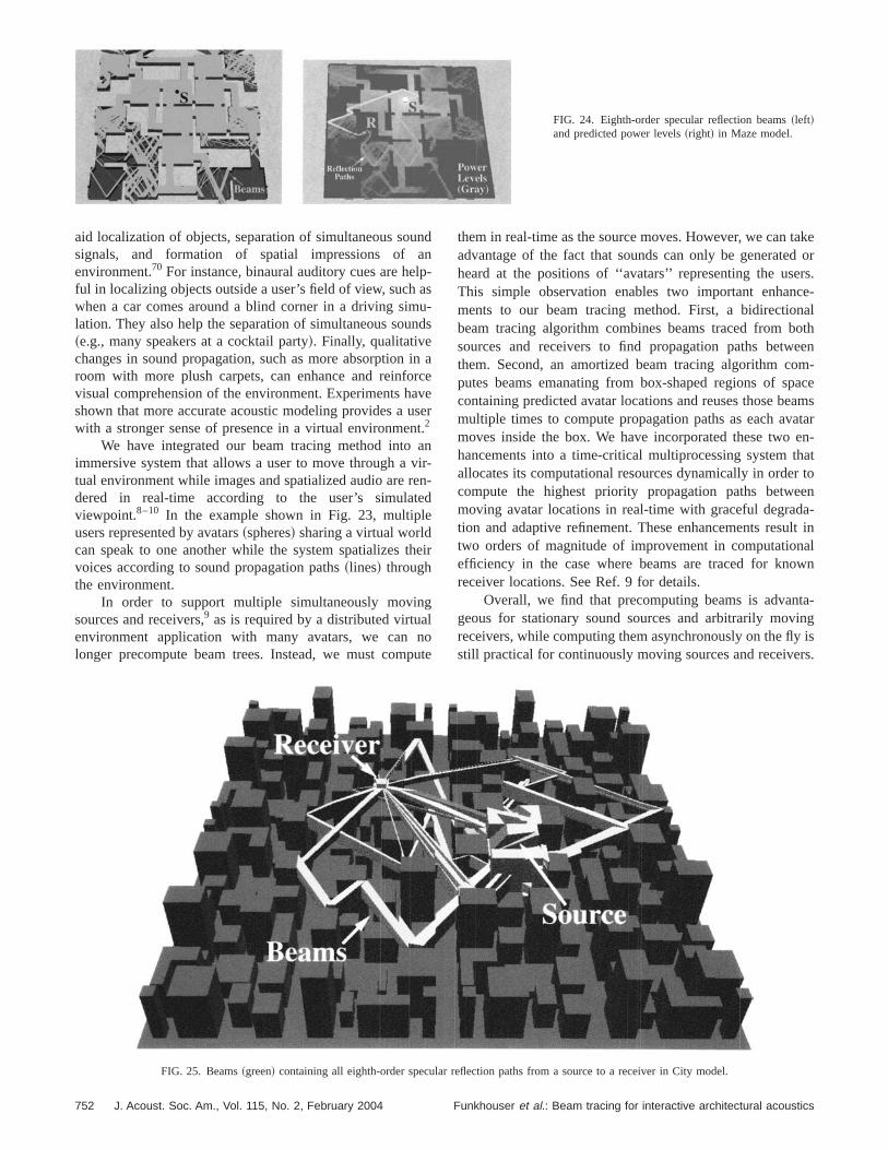
FIG. 24. Eighth-order specular reflection beams~left!and predicted power levels~right! in Maze model.

unanlpaun

inr

avusntaviretee

th

glnpu

taked orrs.ce-nalotheenm-

paceamsataren-hatr toena-lt inalwn

ta-ingy isrs.

aid localization of objects, separation of simultaneous sosignals, and formation of spatial impressions ofenvironment.70 For instance, binaural auditory cues are heful in localizing objects outside a user’s field of view, suchwhen a car comes around a blind corner in a driving simlation. They also help the separation of simultaneous sou~e.g., many speakers at a cocktail party!. Finally, qualitativechanges in sound propagation, such as more absorptionroom with more plush carpets, can enhance and reinfovisual comprehension of the environment. Experiments hshown that more accurate acoustic modeling provides awith a stronger sense of presence in a virtual environme2

We have integrated our beam tracing method intoimmersive system that allows a user to move through atual environment while images and spatialized audio aredered in real-time according to the user’s simulaviewpoint.8–10 In the example shown in Fig. 23, multiplusers represented by avatars~spheres! sharing a virtual worldcan speak to one another while the system spatializesvoices according to sound propagation paths~lines! throughthe environment.

In order to support multiple simultaneously movinsources and receivers,9 as is required by a distributed virtuaenvironment application with many avatars, we canlonger precompute beam trees. Instead, we must com


d

-s-ds

aceeer.nr-n-d

eir

ote

them in real-time as the source moves. However, we canadvantage of the fact that sounds can only be generateheard at the positions of ‘‘avatars’’ representing the useThis simple observation enables two important enhanments to our beam tracing method. First, a bidirectiobeam tracing algorithm combines beams traced from bsources and receivers to find propagation paths betwthem. Second, an amortized beam tracing algorithm coputes beams emanating from box-shaped regions of scontaining predicted avatar locations and reuses those bemultiple times to compute propagation paths as each avmoves inside the box. We have incorporated these twohancements into a time-critical multiprocessing system tallocates its computational resources dynamically in ordecompute the highest priority propagation paths betwemoving avatar locations in real-time with graceful degradtion and adaptive refinement. These enhancements resutwo orders of magnitude of improvement in computationefficiency in the case where beams are traced for knoreceiver locations. See Ref. 9 for details.

Overall, we find that precomputing beams is advangeous for stationary sound sources and arbitrarily movreceivers, while computing them asynchronously on the flstill practical for continuously moving sources and receive

FIG. 25. Beams~green! containing all eighth-order specular reflection paths from a source to a receiver in City model.


out

lgn

,ua

iti

dhatio

r2a

harbnhtioon

oo

thecallyverowopa-

ingse.

as.

eralarforwere-chto

ible

3Dnesralareh aingth

hecu-e,en-

odvi-

s arel ef-the

c-

B. Visualization

In order to aid the understanding and debugging ofacoustic modeling method, we find it extremely valuableuse interactive visualization of our data structures and arithms. Our system provides menu and keyboard commathat may be used to toggle display of the~1! input polygons,~2! source point,~3! receiver point,~4! boundaries of thespatial subdivision,~5! pyramidal beams,~6! image sourcesand ~7! propagation paths. The system also supports visization of acoustic metrics~e.g., power, clarity, etc.! for a setof receiver locations on a regular planar grid displayed wa textured polygon. Example visualizations are shownFigs. 24–26.

Of course, many commercial11–13 and researchsystems29,71provide elaborate tools for visualizing computeacoustic metrics. The critical difference in our system is tit supports continuous interactive updates of propagapaths and debugging information as a user moves theceiver point with the mouse. For instance, Figs. 24 andshow eighth-order specular reflection paths from a singledio source to a receiver location which is updated more tsix times per second as the receiver location is moved atrarily. Figure 27 shows paths with specular reflections adiffractions computed in a city model and an auditorium. Tuser may select any propagation path for further inspecby clicking on it and then independently toggle displayreflecting cell boundaries, transmitting cell boundaries, athe polyhedral beams associated with the selected path.

Separate pop-up windows provide real-time displayother useful visual debugging and acoustic modeling inf

FIG. 26. Impulse response~inset! derived from eighth-order specular refletion paths~yellow! in Floor model.


roo-ds

l-

hn

tne-6u-ni-den

fd

fr-

mation. For instance, one window shows a diagram ofbeam tree data structure. Each beam tree node is dynamicolored in the diagram according to whether the receipoint is inside its associated beam or cell. Another windshows a plot of the impulse response representing the prgation paths from source to receiver~see Fig. 26!. A thirdwindow shows values of various acoustic metrics, includpower, clarity, reverberation time, and frequency responAll of the information displayed is updated in real-timethe user moves the receiver interactively with the mouse

C. Geometric limitations

Our system is a research prototype, and it has sevlimitations. First, the 3D model must comprise only planpolygons because we do not model the transformationsbeams as they reflect off curved surfaces. Furthermore,do not trace beams along paths of refraction or diffuseflection, which may be important acoustical effects. Eaacoustic reflector is assumed to be locally reacting andhave dimensions far exceeding the wavelength of audsound.

Second, our methods are only practical for coarsemodels without highly faceted surfaces, such as the ooften found in acoustic modeling simulations of architectuspaces and concert halls. The difficulty is that beamsfragmented by cell boundaries as they are traced througcell adjacency graph. For this reason, our beam tracmethod would not perform well for geometric models wihigh local geometric complexity~e.g., a forest of trees!.

Third, the major occluding and reflecting surfaces of tvirtual environment must be static through the entire exetion. If any acoustically significant polygon were to movthe cell adjacency graph would have to be updated incremtally.

The class of geometric models for which our methdoes work well includes most architectural and urban enronments. In these cases, acoustically significant surfacegenerally planar, large, and stationary, and the acousticafects of any sound source are limited to a local region ofenvironment~densely occluded!.

he pit and
FIG. 27. Visualizations of sound paths in different environments. Diffraction of sound in a city environment is shown on the left, while early propagation pathsfor a source located in the orchestra pit of an opera house are shown in the middle and right images. Note the diffracted paths over the lip of tbalconies~cyan arrows!.

inlec-d

ng

arlss

acra

tohl adaheiete

na

rif-

nithcit

tlyo

ieicrenthronsi

othhtheellizlas

ounn?uath

tu

dataathstests.es,

epth-

theom arac-con-nson

d iso-e,

Oursu-

wero-ga-ister-lizeng.

isir

-

g

J.

e of

r-

st,als

for

ics

D. Future work

Our system could be extended in many ways. Forstance, the beam tracing algorithm is well suited for paralization, with much of the previous work in parallel ray traing directly applicable.72 Also, the geometric regions covereby each node of the beam tree could be stored in a sihierarchical spatial structure~e.g., a BSP!, allowing logarith-mic search during path generation, rather than linear seof the beams inside a single cell. Of course, we could ause beam trees to allow a user to manipulate the acouproperties of individual surfaces of the environment intertively with real-time feedback, such as for parametrizedtracing73 or for inverse modeling.74

Verification of our simulation results by comparisonmeasured data is an important topic for further study. In tpaper, we have purposely focused on the computationapects of geometrical acoustic modeling and left the valition of the models for future work. For this aspect of tproblem, we refer the reader to related verification stud~e.g., Ref. 75!, noting that our current system can computhe same specular reflection paths as methods based oage sources and ray tracing for which verification resultspublished~e.g., Refs. 76 and 77!.

We are currently making impulse response measuments for verification of our simulations with reflections, dfractions, and transmissions. We have recently built‘‘room’’ for validation experiments. The base configuratioof the room is a simple box. However, it is constructed wreconfigurable panels that can be removed or inserted toate a variety of interesting geometries, including ones wdiffracting panels in the room’s interior. We are currenmeasuring the directional reflectance distribution of eachthese panels in the Anechoic Chamber at Bell LaboratorWe plan to make measurements with speakers and mphones at several locations in the room and with differgeometric arrangements of panels, and we will comparemeasurements with the results of simulations with the pposed beam tracing algorithms for matching configuratio

Perhaps the most interesting direction of future workto investigate the possible applications ofinteractiveacousticmodeling. What can we do with interactive manipulationacoustic model parameters that would be difficult to do oerwise? As a first application, we hope to build a system tuses our interactive acoustic simulations to investigatepsychoacoustic effects of varying different acoustic moding parameters. Our system will allow a user to interactivchange various acoustic parameters with real-time auration and visualization feedback. With this interactive simution system, it may be possible to address psychoacouquestions, such as ‘‘how many reflections are psychoactically important to model?’’ or ‘‘which surface reflectiomodel provides a psychoacoustically better approximatioMoreover, we hope to investigate the interaction of visand aural cues on spatial perception. We believe thatanswers to such questions are of critical importance to fudesign of 3D simulation systems.


-l-

le

chotic-y

iss--

s

im-re

e-

a

re-h

fs.o-te-.

s

f-

ate

l-ya--tics-

’’le

re

VII. CONCLUSION

We have described a system that uses beam tracingstructures and algorithms to compute early propagation pfrom static sources to a moving receiver at interactive rafor real-time auralization in large architectural environmen

As compared to previous acoustic modeling approachour beam tracing method takes unique advantage ofprecom-putation and convexity. Precomputation is used twice, oncto encode in the spatial subdivision data structure a deordered sequence of~cell boundary! polygons to be consid-ered during any traversal of space, and once to encode inbeam tree data structure the region of space reachable frstatic source by sequences of specular reflections, difftions, and transmissions at cell boundaries. We use thevexity of the beams, cell regions, and cell boundary polygoto enable efficient and robust computation of beam-polygand beam-receiver intersections. As a result, our methouniquely able to~1! enumerate all propagation paths rbustly, ~2! scale to compute propagation paths in largdensely occluded environments,~3! model effects of edgediffraction in arbitrary polyhedral environments, and~4! sup-port evaluation of propagation paths at interactive rates.interactive system integrates real-time auralization with vialization of large virtual environments.

Based on our initial experiences with this system,believe that interactive geometric acoustic modeling pvides a valuable new tool for understanding sound propation in complex 3D environments. We are continuing thresearch in order to further investigate the perceptual inaction of visual and acoustical effects and to better reathe opportunities possible with interactive acoustic modeli

ACKNOWLEDGMENTS

The authors thank Sid Ahuja for his support of thwork, and Arun C. Surendran and Michael Gatlin for thevaluable discussions and contributions to the project.

1D. R. Begault,3D Sound for Virtual Reality and Multimedia~Academic,New York, 1994!.

2N. I. Durlach and A. S. Mavor,Virtual Reality Scientific and Technological Challenges, National Research Council Report~National Academy,Washington, D.C., 1995!.

3H. Kuttruff, Room Acoustics (3rd edition)~Elsevier Applied Science, NewYork, 1991!.

4J. B. Allen and D. A. Berkley, ‘‘Image method for efficiently simulatinsmall room acoustics,’’ J. Acoust. Soc. Am.65, 943–950~1979!.

5J. Borish, ‘‘Extension of the image model to arbitrary polyhedra,’’Acoust. Soc. Am.75, 1827–1836~1984!.

6U. R. Krockstadt, ‘‘Calculating the acoustical room response by the usa ray tracing technique,’’ J. Sound Vib.8~18!, 118–125~1968!.

7M. Kleiner, B. I. Dalenback, and P. Svensson, ‘‘Auralization—An oveview,’’ J. Audio Eng. Soc.41~11!, 861–875~1993!.

8T. Funkhouser, I. Carlbom, G. Elko, G. Pingali, M. Sondhi, and J. We‘‘A beam tracing approach to acoustic modeling for interactive virtuenvironments,’’ACM Computer Graphics, SIGGRAPH’98 Proceeding,July 1998, pp. 21–32.

9T. Funkhouser, P. Min, and I. Carlbom, ‘‘Real-time acoustic modelingdistributed virtual environments,’’ACM Computer Graphics, SIG-GRAPH’99 Proceedings, August 1999, pp. 365–374.

10N. Tsingos, T. Funkhouser, A. Ngan, and I. Carlbom, ‘‘Modeling acoustin virtual environments using the uniform theory of diffraction,’’ACMComputer Graphics, SIGGRAPH 2001 Proceedings, August 2001, pp.545–552.


://

l.

lc

eus

.

ion

is

sis

ge

-

l.

amtr

a-

im

enil

ar

u-

is

J.

-

i-ia

,’’

es,

g and

uter

del

Fning

n

nd

al

w-

caln-

e-

ion0

-

el,’’

l.

usa-

d

ed-

of

d

J.

ac-

urce

11Bose Corporation, Bose Modeler, Framingham, MA, httpwww.bose.com.

12CATT-Acoustic, Gothenburg, Sweden, http://www.netg.se/catt.13J. M. Naylor, ‘‘Odeon—Another hybrid room acoustical model,’’ App

Acoust.38~1!, 131–143~1993!.14R. D. Ciskowski and C. A. Brebbia~eds.!, Boundary Element Methods in

Acoustics~Elseiver Applied Science, New York, 1991!.15P. Filippi, D. Habault, J. P. Lefevre, and A. Bergassoli,Acoustics, Basic

Physics, Theory and Methods~Academic, New York, 1999!.16A. Kludszuweit, ‘‘Time iterative boundary element method~TIBEM!—a

new numerical method of four-dimensional system analysis for the calation of the spatial impulse response,’’ Acustica75, 17–27 ~1991! ~inGerman!.

17S. Kopuz and N. Lalor, ‘‘Analysis of interior acoustic fields using thfinite element method and the boundary element method,’’ Appl. Aco45, 193–210~1995!.

18G. R. Moore, ‘‘An Approach to the Analysis of Sound in Auditoria,’’ Ph.Dthesis, Cambridge, UK, 1984.

19N. Tsingos and J.-D. Gascuel, ‘‘Soundtracks for computer animatSound rendering in dynamic environments with occlusions,’’GraphicsInterface’97, May 1997, pp. 9–16.

20M. F. Cohen and J. R. Wallace,Radiosity and Realistic Image Synthes~Academic, New York, 1993!.

21F. X. Sillion and C. Puech,Radiosity and Global Illumination~MorganKaufmann, San Francisco, 1994!.

22K. H. Kuttruff, ‘‘Auralization of impulse responses modeled on the baof ray-tracing results,’’ J. Audio Eng. Soc.41~11!, 876–880~1993!.

23U. R. Kristiansen, A. Krokstad, and T. Follestad, ‘‘Extending the imamethod to higher-order reflections,’’ J. Appl. Acoust.38~2-4!, 195–206~1993!.

24R. Cook, T. Porter, and L. Carpenter, ‘‘Distributed ray-tracing,’’ACMComputer Graphics, SIGGRAPH’84 Proceedings, July 1984, Vol. 18~3!,pp. 137–146.

25J. T. Kajiya, ‘‘The rendering equation,’’ACM Computer Graphics, SIGGRAPH’86 Proceedings, Vol. 20~4!, pp. 143–150.

26H. Lehnert, ‘‘Systematic errors of the ray-tracing algorithm,’’ AppAcoust.38, 207–221~1993!.

27N. Dadoun, D. G. Kirkpatrick, and J. P. Walsh, ‘‘The geometry of betracing,’’ Proceedings of the Symposium on Computational Geome,June 1985, pp. 55–71.

28P. Heckbert and P. Hanrahan, ‘‘Beam tracing polygonal objects,’’ACMComputer Graphics, SIGGRAPH’84 Proceedings, Vol. 18~3!, pp. 119–127.

29M. Monks, B. M. Oh, and J. Dorsey, ‘‘Acoustic simulation and visualistion using a new unified beam tracing and image source approach,’’Proc.Audio Engineering Society Convention, 1996, pp. 153–174.

30U. Stephenson and U. Kristiansen, ‘‘Pyramidal beam tracing and tdependent radiosity,’’Fifteenth International Congress on Acoustics, June1995, pp. 657–660.

31J. P. Walsh and N. Dadoun, ‘‘What are we waiting for? The developmof Godot, II,’’ 103rd Meeting of the Acoustical Society of America, Apr1982.

32J. H. Chuang and S. A. Cheng, ‘‘Computing caustic effects by backwbeam tracing,’’ Visual Comput.11~3!, 156–166~1995!.

33A. Fujomoto, ‘‘Turbo beam tracing—A physically accurate lighting simlation environment,’’Knowledge Based Image Computing Systems, May1988, pp. 1–5.

34G. Ghazanfarpour and J. M. Hasenfratz, ‘‘A beam tracing with precantialiasing for polyhedral scenes,’’ Comput. Graph.22~1!, 103–115~1998!.

35E. Haines, ‘‘Beams O’ Light: Confessions of a hacker,’’Frontiers in Ren-dering, Course Notes, SIGGRAPH’91, 1991.

36M. Watt, ‘‘Light-water interaction using backward beam tracing,’’ACMComputer Graphics, SIGGRAPH’90 Proceedings, August 1990, pp. 377–385.

37C. B. Jones, ‘‘A new approach to the ‘hidden line’ problem,’’ Comput.14~3!, 232–237~1971!.

38T. Funkhouser, ‘‘A visibility algorithm for hybrid geometry- and imagebased modeling and rendering,’’ Comput. Graph.23~5!, 719–728~1999!.

39S. Teller, ‘‘Visibility Computations in Densly Occuded Polyhedral Envronments,’’ Ph.D. thesis, Computer Science Div., University of CalifornBerkeley, 1992.

40S. Fortune, ‘‘Algorithms for prediction of indoor radio propagation


u-

t.

:

y

e

t

d

e

,

Technical Report Document 11274-960117-03TM, Bell Laboratori1996.

41S. J. Fortune, ‘‘Topological beam tracing,’’ inProc. 15th ACM Symposiumon Computational Geometry, 1999, pp. 59–68.

42J. Amanatides, ‘‘Ray tracing with cones,’’ACM Computer Graphics, SIG-GRAPH’84 Proceedings, July 1984, Vol. 18~3!, pp. 129–135.

43J. P. Vian and D. van Maercke, ‘‘Calculation of the room response usinray tracing method,’’Proceedings of the ICA Symposium on Acoustics aTheater Planning for the Performing Arts, 1986, pp. 74–78.

44T. Lewers, ‘‘A combined beam tracing and radiant exchange compmodel of room acoustics,’’ Appl. Acoust.38, 161–178~1993!.

45P. Kreuzgruber, P. Unterberger, and R. Gahleitner, ‘‘A ray splitting mofor indoor radio propagation associated with complex geometries,’’ inPro-ceedings of the 1993 43rd IEEE Vehicular Technology Conference, 1993,pp. 227–230.

46A. Rajkumar, B. F. Naylor, F. Feisullin, and L. Rogers, ‘‘Predicting Rcoverage in large environments using ray-beam tracing and partitiotree represented geometry,’’ Wireless Networks2~2!, 143–154~1996!.

47S. Teller and P. Hanrahan, ‘‘Global visibility algorithms for illuminatiocomputations,’’ pp. 239–246~1993!.

48S. Teller, C. Fowler, T. Funkhouser, and P. Hanrahan, ‘‘Partitioning aordering large radiosity computations,’’ACM Computer Graphics, SIG-GRAPH’93 Proceedings, August 1994, pp. 443–450.

49P. Min and T. Funkhouser, ‘‘Priority-driven acoustic modeling for virtuenvironments,’’EUROGRAPHICS 2000, August 2000, pp. 179–188.

50F. Durand, G. Drettakis, and C. Puech, ‘‘The visibility skeleton: A poerful and efficient multi-purpose global visibility tool,’’ inComputerGraphics, SIGGRAPH’97 Proceedings, 1997, pp. 89–100.

51B. G. Baumgart, ‘‘Winged edge polyhedron representation,’’ TechniReport AIM-179 ~CS-TR-74-320!, Computer Science Department, Staford University, Palo Alto, CA, October 1972.

52D. P. Dobkin and M. J. Laszlo, ‘‘Primitives for the manipulation of thredimensional subdivisions,’’ Algorithmica4~1!, 3–32~1989!.

53H. Fuchs, Z. M. Kedem, and B. F. Naylor, ‘‘On visible surface generatby a priori tree structures,’’ACM Computer Graphics, SIGGRAPH ’8Proceedings, July 1980, Vol. 14~3!, pp. 124–133.

54B. F. Naylor, ‘‘Constructing good partitioning trees,’’Graphics Inter-face’93, May 1993, pp. 181–191.

55J. B. Keller, ‘‘Geometrical theory of diffraction,’’ J. Opt. Soc. Am.52~2!,116–130~1962!.

56S. Teller, ‘‘Computing the antiumbra cast by an area light source,’’ACMComputer Graphics, SIGGRAPH’92 Proceedings, July 1992, Vol. 26~2!,pp. 139–148.

57J. Goodman and J. O’Rourke~eds.!, Handbook of Discrete and Computational Geometry~CRC, Boca Raton, FL, 1997!.

58W. Press, S. Teukolsky, W. Vetterling, and B. Flannery,Numerical Recipesin C, 2nd edition~Cambridge U.P., New York, 1992!.

59L. Aveneau, Y. Pousset, R. Vauzelle, and M. Me´riaux, ‘‘Development andevaluations of physical and computer optimizations for the 3d utd modAP2000 Millennium Conference on Antennas & Propagation~Poster!,April 2000.

60H. Lehnert and J. Blauert, ‘‘Principles of binaural room simulation,’’AppAcoust.36, 259–291~1992!.

61M. E. Delany and E. N. Bazley, ‘‘Acoustical characteristics of fibroabsorbent materials,’’ Technical Report NPL AERO REPORT Ac37, Ntional Physical Laboratory, Aerodynamics Division, March 1969.

62A. D. Pierce,Acoustics. An introduction to its physical principles anapplications, 3rd ed.~American Institute of Physics, New York, 1984!.

63S.-I. Thomasson, ‘‘Reflection of waves from a point source by an impance boundary,’’ J. Acoust. Soc. Am.59, 780–785~1976!.

64R. G. Kouyoumjian and P. H. Pathak, ‘‘A uniform geometrical theorydiffraction for an edge in a perfectly conducting surface,’’ Proc. IEEE62,1448–1461~1974!.

65T. Kawai, ‘‘Sound diffraction by a many sided barrier or pillar,’’ J. SounVib. 79~2!, 229–242~1981!.

66M. A. Biot and I. Tolstoy, ‘‘Formulation of wave propagation in infinitemedia by normal coordinates with an application to diffraction,’’Acoust. Soc. Am.29, 381–391~1957!.

67H. Medwin, E. Childs, and G. Jebsen, ‘‘Impulse studies of double diffrtion: A discrete huygens interpretation,’’ J. Acoust. Soc. Am.72, 1005–1013 ~1982!.

68U. P. Svensson, R. I. Fred, and J. Vanderkooy, ‘‘Analytic secondary somodel of edge diffraction impulse responses,’’ J. Acoust. Soc. Am.106,2331–2344~1999!.


geoc

a

fod-

d

ters-

alroom

ithg

69R. R. Torres, U. P. Svensson, and M. Kleiner, ‘‘Computation of eddiffraction for more accurate room acoustics auralization,’’ J. Acoust. SAm. 109, 600–610~2001!.

70J. Blauert,Spatial Hearing: The Psychophysics of Human Sound Locization ~MIT, Cambridge, MA, 1983!.

71A. Stettner and D. P. Greenberg, ‘‘Computer graphics visualizationacoustic simulation,’’ACM Computer Graphics, SIGGRAPH’89 Proceeings, July 1989, Vol. 23~3!, pp. 195–206.

72J. Arvo and D. Kirk, ‘‘A survey of ray tracing acceleration techniques,’’AnIntroduction to Ray Tracing, 1989.

73C. Sequin and E. Smyrl, ‘‘Parameterized ray tracing,’’ACM ComputerGraphics, SIGGRAPH’89 Proceedings, July 1989, Vol. 23~3!, pp. 307–314.


.

l-

r

74M. Monks, B. M. Oh, and J. Dorsey, ‘‘Audioptimization: Goal baseacoustic design,’’IEEE Computer Graphics & Applications, May 2000,pp. 76–91.

75M. Vorlander, ‘‘International round robin on room acoustical compusimulations,’’ inProceedings of the 15th International Congress of Acoutics, June 1995.

76K. Nakagawa, T. Miyajima, and Y. Tahara, ‘‘An improved geometricsound field analysis in rooms using scattered sound and an audibleacoustic simulator,’’ J. Appl. Acoust.38~2-4!, 115–130~1993!.

77G. M. Naylor and J. H. Rindel, ‘‘Predicting room acoustical behavior wthe odeon computer model,’’ inProceedings of the 124th ASA Meetin,November 1992, p. 3aAA3.


Documents

A beam tracing method for interactive architectural …people.csail.mit.edu/addy/research/funk-beamtracing-jasa04.pdf · Avaya Labs, Basking Ridge, New Jersey 07920 James E. West