A BAYESIAN SYSTEM FOR MODELING PROMOTER

STRUCTURE: A CASE STUDY OF HISTONE PROMOTERS

RAJESH CHOWDHARY (MSc & DIC, Imperial College, London)

A THESIS SUBMITTED

FOR THE DEGREE OF DOCTOR OF PHILOSOPHY

SCHOOL OF COMPUTING

NATIONAL UNIVERSITY OF SINGAPORE

2006

i

ACKNOWLEDGEMENTS

I would like to express my sincere gratitude to my supervisor Professor Vladimir B Bajic

for his invaluable guidance and providing me inspiration to work on the problems of this

thesis. I am grateful to him for his patience, support and understanding in helping me

balance my personal life with my research during my PhD. I have specially enjoyed the

freedom given by him, which inculcated independent thinking in me in the field of

Bioinformatics. It has been a pleasure working with him.

My heartfelt gratitude to my supervisor Professor Limsoon Wong for his continued

guidance, encouragement and support, particularly at the critical junctures. His quotes

have been truly inspiring. With deep appreciation I would like to extend my warmest

thanks to him.

I would also like to extend my sincere thanks to Dr Rebecca A Ali for providing me

invaluable guidance and support during the course of my Phd.

I am also grateful to our German collaborators, Professor Detlef Doenecke and Professor

Werner Albig, for providing useful information and guidance on histone genes.

I am also thankful to my committee members Dr. Ken Sung and Dr. Roland Yap for

providing me useful suggestions during my presentations.

My sincere thanks to Brent Boerlage, Norsys Software Corp. for providing me Netica

library free of charge. I am also grateful to my colleagues Sin Lam Tan, Vipin Narang,

and Zhang Zhuo for being great supportive friends all along. I also thank School of

Computing and Institute for Infocomm Research for supporting me for my studies.

My sincere thanks to Professor Jun Liu and Department of Statistics at Harvard

University for kindly supporting the end stages of my thesis work.

Finally, I am thankful to my parents, wife Vidhu and son Advait "Google" for providing

me moral support and for being patient with me.

ii

TABLE OF CONTENTS

Acknowledgements i

List of Tables iv

List of Figures v

List of Abbreviations and Notations vi

List of Publications viii

Summary ix

Page

1. Introduction ..1

2. Biological Background ..7

2.1 Regulation of Gene expression and Promoter ..7

2.2 Why is it difficult to model promoters computationally? ..11

2.3 Promoter modeling tools and resources ..12

3. Specific aspects related to research project ..18

3.1 Histone Basics ..18

3.2 Bayesian Networks ..19

4. Research Project ..25

4.1 Research problems ..25

4.2 Work done ..27

4.2.1 Elucidation of histone promoter content ..27

4.2.2 Dragon Promoter Mapper [DPM] – a promoter modeling system ..32

4.2.3 Modeling of promoter structure of human histone genes using DPM ..39

4.2.4 Comparative analysis of DPM’s performance and several other systems ..47

4.2.5 Human genome scan using human histone promoter structure model ..52

5. Conclusion ..64

iii

References ..66

Appendices

Appendix A ..78

A.1 Input and output files for the DPM system ..78

A.2 Model comparison analysis ..83

A.3 Files related to human genome analysis using histone promoter model ..83

A.4 How the long sequence processing module works? ..83

A.5 Predicted histone co-regulated/co-expressed genes ..84

A.6 Histone gene prediction at probability > 0.9 ..86

iv

LIST OF TABLES

Page

Table 4.1: Relationship between detected motifs in histone promoters and biologically verified TFBS obtained from TRANSFAC database ..29 Table 4.2: Performance of histone promoter structure Bayesian models with different DAG structures ..45 Table 4.3: Performance of motif cluster finding programs ..48

Table 4.4: Motif distribution/arrangement within the clusters reported by the compared programs in five histone promoter sequences ..50 Table 4.5: Performance of general promoter prediction programs ..51

Table 4.6: Human genome analysis with histone promoter model using DPM ..61

Table 4.7: Positional bias between DPM predictions and gene transcript locations ..62

Table 4.8: Overlapping/redundancy in DPM predictions that are classified as histone class ..63 Table 4.9: Number of DPM predictions on probability scale ..63

v

LIST OF FIGURES

Page

Fig 2.1: Stages of gene expression in cell ..8

Fig 2.2: A typical promoter structure showing modular organization of TFBSs ..11

Fig 3.1: A Bayesian Network showing four nodes and their associated CPTs ..21

Fig. 4.1: Relative presence of motifs in different histone groups ..30

Fig 4.2: Schematic of DPM workflow ..35

Fig 4.3: Example of a Bayesian network model of promoter structure with four motif positions ..37 Fig. 4.4: DAG structures for Bayesian networks used for modeling histone promoter ..46 Fig. 4.5: Predicted Screenshot of DAVID showing biological terms shared by 1334 DPM predicted histone co-regulated genes ..59

vi

LIST OF ABBREVIATIONS AND NOTATIONS

TFBS - Transcription factor binding site

TSS - Transcription start site

TF - Transcription factor

DPM - Dragon promoter mapper

NCBI - National Center for Biotechnology Information

EMBL - European Molecular Biology Laboratory

DDBJ - DNA Data Bank of Japan

DNA - Deoxyribonucleic acid

RNA - Ribonucleic acid

mRNA - Messenger RNA

IHGSC - International Human Genome Sequencing Consortium

bp - Base pair

A, C, G, T - Nucleotides/bases

PWM - Position weight matrix

EM - Expectation maximization

HMM - Hidden Markov Model

H1, H2A, H2B, H3, H4 - Five histone classes

DAG - Directed acyclic graph

CPD - Conditional probability distribution

CPT - Conditional probability table

HOMD – Higher order motif definition

Mi - Motif at position i

Si - Strand at position i

L(i+1)_i - Mutual length between motifs at positions i and i+1

TP - True positive

vii

FP - False positive

Se - Sensitivity

ppv - Positive predicted value

cc - Correlation coefficient

stdev – Standard deviation

P(C, S, R, W) - Joint probability of nodes C, S, R and W

P(C) - Marginal probability of node C

P(S|C) - Conditional probability of node S given C

P(W|S,R) - Conditional probability of node W given nodes S and R

P(R=T|W=T) - Probability of R being True, given that W is True

H0 - A hypothesis.

P(H0) - Prior probability of H0

P(E|H0) - Conditional probability of observing the evidence E given that the hypothesis

H0 is true.

P(E) - Marginal probability of E

P(H0|E) - Posterior probability of H0 given E

MCMC – Markov Chain Monte Carlo

viii

LIST OF PUBLICATIONS

• R Chowdhary, SL Tan, RA Ali, B Boerlage, L Wong, VB Bajic. Dragon

Promoter Mapper (DPM): a Bayesian framework for modeling promoter

structures. Bioinformatics, Apr 2006 (Epub ahead of print). PMID: 16613910.

• R Chowdhary, L Wong, VB Bajic. Finding functional promoter motifs by

computational methods: a word of caution. International Journal of

Bioinformatics Research and Applications (IJBRA), accepted.

• R Chowdhary, RA Ali, W Albig, D Doenecke, VB Bajic. Promoter modeling:

the case study of mammalian histone promoters, Bioinformatics, 21(11):2623-8,

2005. PMID: 15769833.

• E Huang, L Yang, R Chowdhary, A Kassim, VB Bajic. An algorithm for ab

initio DNA motif detection, Chapter 4 in Information Processing and Living

Systems, World Scientific, 611-4, 2005.

• R Chowdhary, RA Ali, VB Bajic. Modeling 5' regions of histone genes using

Bayesian networks. Asia-Pacific Bioinformatics Conference (APBC) 283-8, 2005.

• M Brahmachary, C Schönbach, L Yang, E Huang, SL Tan, R Chowdhary, SPT

Krishnan, CY Lin, DA Hume, C Kai, J Kawai, P Carninci, Y Hayashizaki, VB

Bajic. Computational Promoter Analysis of Mouse, Rat and Human

Antimicrobial Peptide-coding Genes. BMC Bioinformatics, 7(5):S8, 2006.

• V Narang, R Chowdhary, A Mittal, WK Sung. Bayesian network modeling of

transcription factor binding sites a book chapter in: Bayesian Network

Technologies: Applications and Graphical Models, Idea Group Publishing,

Pennsylvania, USA 2006.

• R Chowdhary, L Wong, VB Bajic. Recognition of genes co-regulated with

histone genes on a genome-wide scale. Under preparation.

ix

SUMMARY

Gene regulation has been recognized as an important line of research due to its crucial

biological significance. Very little is known about gene regulatory mechanisms till date.

One of the essential regulatory regions of the gene is its promoter region. Recognition and

annotation of promoter regions besides other regulatory regions in the genomes remains a

fundamental task even today. This is because the genomic data continue to stay largely

unannotated, particularly the regulatory regions. One reason that can be attributed to this

problem is that promoter recognition and annotation is an extremely challenging problem

in part due to the complexity of the data involved.

Promoter modeling, a term used interchangeably with promoter recognition and

annotation, can be performed using experimental techniques. However, due to the huge

size of genomic data involved, computational techniques have become a good

compliment alongside. Researchers in the past have proposed many computational

promoter modeling approaches, most of which have primarily been focused towards

general promoter recognition. However, these programs not only generally suffer from

high number of false positives but also appear too general to faithfully model all classes

of promoters together. Promoters of different classes generally have too little in common

to be described by a single promoter model. Another type of programs that perform better

are specific promoter recognition programs, which focus on modeling a particular class of

promoters. Still, specific promoter recognition approaches have received relatively less

focus compared to general promoter recognition programs, perhaps due to unavailability

of sufficient, relevant and clean data of different classes of promoters. The present study

is an attempt in this direction. My PhD project is aimed at modeling and recognition of

specific promoter structures, which has till date received only partial success. I have

focused explicitly on histone protein-coding genes. Histones are an important class of

x

proteins that play a crucial role in various cellular functions related to gene transcription

and regulation.

I have proposed a novel computational methodology based on Bayesian networks to

model promoter structures of histone genes based on the properties of regulatory signals

present in them. Using the developed histone promoter model, my methodology attempts

to discover the regions in the human genome that have structures similar to histone

promoter model; such regions may in part represent promoters of the genes that may

potentially be coregulated with histone genes. My methodology is a general-purpose

framework to model promoter structures of any class of genes. The methodology has been

shown to perform better than several other similar well-known programs. It has certain

distinct advantages compared to the other related systems that have been highlighted in

the text. The results obtained in this study have been found to be statistically significant

and have been validated with experimental data.

To the best of my knowledge this is the first comprehensive study that has attempted to

systematically computationally model histone promoter structures. Overall, the present

study has resulted in the development of, i) Dragon promoter mapper (DPM), a tool to

model promoter structures of a particular class of genes, and ii) annotated data of histone

promoter models, that compliments just a handful of datasets known to the research

community for which specific promoter models have been studied, and iii) data of human

genomic regions that have similar structures as histone promoters.

I hope these tools and data would prove to be useful to the research community.

1

1. INTRODUCTION

Biological studies can be performed by experimental wet-lab techniques. However, these

techniques can be very expensive and time consuming. The experimental techniques therefore are

not suited to handle huge amounts of genomic data, such as those that are present in the public

databases of NCBI (http://www.ncbi.nlm.nih.gov/), EMBL (http://www.ebi.ac.uk/embl/) and

DDBJ (http://www.ddbj.nig.ac.jp/) and others. Thus, there is a need for computational techniques

that can be applied on the large genomic datasets, with the aim to verify the results so obtained by

experiments later. Such pragmatic considerations have introduced the field of Bioinformatics.

Bioinformatics has been established in the last 20 years as one of the most interdisciplinary fields

of scientific and technological research that involves several disciplines such as computer

science, molecular biology, genetics, and chemistry among others. Loosely speaking,

bioinformatics attempts to provide answers to biological questions based on computational

analysis of biological data. To make efficient bioinformatics solutions there must be a successful

synergy between,

i) biological background understanding of the problem,

ii) biological data understanding,

iii) data conversion into forms appropriate for modeling of the underlying problem, and

iv) computer science type of solution to the problem.

This is why it is sometimes difficult to make strict boundaries between biology and computer

science. From the viewpoint of computer scientists it is of interest to expand the current

application domains of the existing technologies to new and exciting areas of life sciences. This

study represents a step in this direction, attempting to apply a computer science technology to a

difficult yet exciting functional genomics problem of gene regulation.

2

The difference between man and monkey is gene regulation. - by Leroy Hood (quoted in

Werner 2001).

The above quote highlights the importance of gene regulation in the very existence of life forms.

Still, much is unknown about it in general. Gene regulation is a complex mechanism that

determines which all genes would express in a particular cell at a particular time and by how

much. Such differential gene expression characteristics are essential for normal functioning of

cells in an organism. Though there have been many studies in the past to computationally unravel

gene regulatory mechanisms, this field is still wide open and much work needs to be done. A

crucial player in gene regulation, that has been the focus of many gene regulation studies, is the

promoter region of the gene. Promoter is a regulatory region on the DNA that covers the start of

the associated gene which is known as transcription start site (TSS), and contains a set of

"switches" or transcription factor binding sites (TFBSs) where particular proteins or a

combination of proteins known as transcription factors (TFs) interact in a specific manner and

regulate the initiation of gene expression process temporally and spatially in the body.

Promoter modeling has been recognized as an important line of research (Fickett and

Hatzigeorgiou 1997, Werner 1999, 2003) due to its crucial biological significance. However, due

to a variety of reasons as highlighted later in the text, promoter modeling is an extremely

challenging problem. Researchers in the recent past have commonly employed computational

tools to perform promoter modeling which largely involves characterization and recognition of

promoters. While characterization involves annotating the structures and the associated regulatory

functions of known promoter sequences, recognition of promoters involves detecting previously

unknown promoter sequences from across the genomes. In characterization, for example,

programs have been built that discover TFBSs and other structurally and functionally important

3

signals in the promoter sequences. Then there are sequence alignment programs that are used to

detect homology between input promoter sequences by aligning them multiply (Higgins et. al.

1994) or in pairs (Altschul et. al. 1990). Promoter recognition programs, on the other hand, aim to

search for novel promoters from across various genomes. These programs have often exploited

the fact that promoters cover the TSSs of their respective genes. A novel promoter detected from

the genome may potentially help in gene discovery. The motivation behind promoter modeling is

therefore usually characterization/annotation of genome data. Genome data remain largely

uncharacterized even today, particularly with regard to annotation of regulatory regions such as

promoters and their functions. The reason for this may be attributed to the complexity of the

problem. For example, human genome comprises 3 billion base pairs and genes and their

regulatory regions are believed to form a very small fraction of this number. Thus, the problem is

like searching a needle from a haystack.

Based on the objectives, promoter modeling techniques can be divided into two broad categories,

namely, general promoter modeling and specific promoter modeling. General promoter modeling

focuses on building computational tools to model all promoters together, while, specific promoter

modeling focuses on building computational tools to model particular class of promoters. For

example, general promoter modeling may involve building models based on general promoter

structure properties of all known promoters together, while specific promoter modeling may

involve building models based on promoter structure properties of a class of promoters, such as

muscle specific gene promoters. Models built on both techniques can be used to scan the genome

and recognize putative promoters that match the promoter properties defined by the models.

Based on these two techniques, many computational strategies have been proposed in the past to

recognize putative promoter regions of DNA (Fickett and Hatzigeorgiou 1997, Werner 1999,

2003, Pedersen et. al. 1999), however these programs have generally suffered from high number

4

of false positives. The fact is that at this moment there is no computer program which can predict

eukaryotic promoters very efficiently (Bajic and Seah 2003a).

Relatively, specific promoter recognition programs show better specificity compared to general

promoter recognition programs (Werner 1999). Still, specific promoter recognition programs

have received relatively less focus compared to general promoter recognition programs, perhaps

due to unavailability of sufficient, relevant and clean data. Apparently, building a single

methodology catering to all types of promoters together appears not only too general but also

highly complex and unrealistic. Various promoter sequences have too little in common to be

described by a single promoter model. A more prudent yet challenging approach is to thus focus

on methodologies that address specific classes of promoters. Additionally, there are other

advantages of specific promoter recognition programs over general promoter prediction

programs, such as in (i) determining the tissue specificity of genes, (ii) predicting the function of

genes, and (iii) identifying co-regulated genes. Such information is presently available for only a

very small fraction of genes.

My PhD research project is aimed at the problem of modeling and recognition of specific

promoter structures, which has till date received only partial success. The project involves

developing a methodology to model promoters of any particular class of genes. I have focused

explicitly on human protein-coding genes, and within this broad class on a special group of genes

which produce histone proteins. Histones are an important class of proteins that play a crucial role

in various cellular functions related to gene transcription and regulation. This focused approach

allowed me to utilize specific properties which many of the promoters of this class share.

I have proposed a novel computational methodology to model promoter structures of histone

genes based on the properties of regulatory signals present in them. Using the developed histone

5

promoter model, my methodology attempts to discover the regions in the human genome that are

structurally similar to histone promoter model; such regions may represent promoters of the genes

that are potentially co-regulated with histone genes.

I have used Bayesian networks to model histone promoter structure, though there could possibly

be many other approaches. Bayesian networks offer a natural way to represent probabilistic data

(Jensen 2001). As highlighted later in the text, biological data are prone to sequencing and

annotation errors due to various reasons and histone promoter data are no exception. The errors in

such data lead to uncertainties that can be aptly handled by the probabilistic framework of

Bayesian networks.

To the best of my knowledge this is the first comprehensive study that has attempted to

systematically computationally model histone promoter structures. The study has also attempted

to discover genes across the human genome that are co-regulated with histone genes. To date

there are only a handful of datasets known to the research community for which specific promoter

models have been studied. These include the sets of i) glucocorticoid and heat-shock responsive

genes (Claverie and Sauvaget 1985), ii) globin family promoters (Staden 1988), iii) muscle

specific genes (Wasserman and Fickett 1998, Klingenhoff et. al. 2002), and iv) liver specific

genes (Krivan and Wasserman 2001). This study contributes another well-annotated dataset to

the research community. As highlighted later in Chapter 5, the DPM system that I have developed

for modeling histone promoter structure has distinct advantages compared to the other related

systems. DPM has shown better performance (Chowdhary et. al. 2006) in terms of sensitivity and

specificity of promoter prediction. It can analyze multiple subtypes of promoter sequences within

a given promoter class. DPM also allows the user to incorporate biological background

knowledge in the model. Aside, DPM is not rigid and the user can flexibly develop and test his

model according to his suitability. DPM methodology is generic and can be applied to model

6

promoters of any class of genes or co-regulated genes. Overall, DPM provides a robust

methodology that can principally be applied for general purpose modeling of structures of any

regulatory region including promoter.

My presentation is divided as follows: The biological background relevant to the problem in

question is in Chapter 2 with sub sections on, i) Regulation of Gene expression and Promoter, ii)

Difficulty in modeling promoters computationally, iii) Promoter modeling tools and resources.

Chapter 3 discusses specific aspects related to research project such as histone basics and

Bayesian networks. Chapter 4 introduces my PhD research problem and work done. The section

on work done has sub sections of, i) Elucidation of histone promoter content, ii) Dragon Promoter

Mapper (DPM) - a promoter structure modeling system, iii) Modeling of promoter structure of

human histone genes using DPM, iv) Comparative analysis of DPM's performance and several

other systems, v) Human genome scan using human histone promoter structure model. The thesis

completes with a conclusion in Chapter 5.

7

2. BIOLOGICAL BACKGROUND

A eukaryotic organism contains the complete genome in the nuclei of most of the cells. The

genome is the complete set of genetic information inherited from the parents and comprises all

the genes. The genome is physically present in the form of a polymer called DNA (deoxyribose

nucleic acid). The basic unit of DNA is a nucleotide which comprises sugar-phosphate backbone

and one of the four bases adenine (A), cytosine (C), guanine (G) and thymine (T). The genetic

instructions encoded in genomic sequences are very less understood. The human genome, for

example, is extraordinarily complex. The protein-coding bases of its 30,000 genes span only less

than 2% of the entire 3 billion base pairs long genomic sequence (IHGSC). Of the rest non-

coding segment of the genome, another small part contains regulatory regions controlling the

expression of these genes. Very little is known regarding these functional regulatory regions.

2.1 Regulation of Gene expression and Promoter

Genes in DNA act as a blueprint for the production of RNA and proteins (another polymer) inside

the cells. Proteins play an essential role in cellular functions. A vast majority of genes are known

to produce proteins as their end products. The process of synthesizing proteins in cells is known

as gene expression. Gene expression involves transfer of sequential genetic information from

DNA to proteins and broadly involves following stages (Fig. 2.1):

i) transcription, where a gene's DNA sequence is transcribed into a single stranded

sequence of primary transcript or pre-mRNA.

ii) capping, where primary transcript is capped on the 5' end, which stabilizes the

transcript by protecting it from degradation enzymes.

iii) poly-adenylation, where a part of 3' end of the primary transcript is replaced by a

poly-A tail for providing stability.

8

iv) splicing, where introns are removed from the primary transcript to form messenger

RNA (mRNA).

v) mRNA is transported from nucleus to cytoplasm.

vi) translation, where a ribosome produces a protein by using the mRNA template.

Fig 2.1: Stages of gene expression in cell.

Gene expression is a strictly regulated process in cells. The regulation of gene expression is

important as it determines where (cell-type), when (developmental stage), how, and in what

quantities various proteins are produced in cells. This decides how cells develop, differentiate and

respond to external stimuli. The detailed mechanism of gene regulation, however, still remains

unclear. Gene regulation occurs at various stages of gene expression from transcription to

translation (stages shown above), though transcription is generally believed to be the most

important stage. The transcription stage of gene expression involves regulatory DNA regions

known as promoters.

Every gene has at least one promoter that mediates and controls its transcription initiation. This

control mechanism occurs through a complex interaction between various TFs that get attached to

9

their specific TFBSs present in the gene's promoter region. A promoter is usually defined as a

non-coding region of DNA that covers the TSS or the 5' end of the gene. Bulk of promoter region

typically lies upstream of the TSS. The promoter region in Eukaryotes is usually difficult to

characterize because of high variability. For example, promoters may vary from a few hundred

bases in some genes to several kilo bases in the others. A promoter may be typically classified as,

i) Core promoter

usually lies up to 30 bp upstream with respect to the TSS

contains the TSS

contains binding site for RNA polymerase

contains general binding sites (i.e. binding sites commonly found in many

promoter types)

example of a binding site in this region is TATA-box

ii) Proximal promoter

usually lies between 200 bp to 300 bp upstream with respect to the TSS

contains specific binding sites that control temporal and spatial expression of a

gene

example of a binding site in this region is CAAT-box

iii) Distal promoter

lies upstream of the proximal promoters, may be located thousands of bases away

from the TSS

contains specific binding sites that control temporal and spatial expression of a

gene

10

Aside a promoter, there are some additional regulatory regions on the DNA that work cohesively

with the promoter in regulating a gene at the transcription stage. These regions are usually located

thousands of bases upstream or downstream of the TSS and regulate the rate of transcription of

the associated gene. Alike promoters, the regulation here also occurs through specific regulatory

TFBSs present in these regions. Examples of such regions include enhancers, silencers and

boundary elements; enhancers increase the gene's transcription rate while silencers decrease it.

Promoter regions are interspersed with characteristic short TFBSs patterns (~6-20 bp in length)

that provide functionality to these regions. These patterns are usually conserved across species

and are degenerate in nature. As TFBS motifs are short they tend to occur frequently anywhere in

the genome, however, only those that are present in the regulatory regions of the genome may be

functionally active. TFBSs show large variations across promoters of a species; some promoters

may have particular TFBSs that others do not have. Between promoters, TFBSs do not

intrinsically have any bias towards a particular location or orientation (Werner 1999). However

for a particular class of promoters such a bias may be observed (Wasserman and Fickett 1998).

Adding to the complexity, the nature of function of a TFBS may depend on its context/location

within the promoter. For example, the factor AP1 suppresses gene transcription when it binds to

its binding site in the distal promoter, while it supports the transcription when it binds to its

binding site in the core promoter (Werner 1999). Such contextual behavior of a TFBS may be

dictated by factors such as, tissue specificity, and cell-cycle & developmental stage. Overall,

there are large variations in TFBS distributions across promoters and their associated functions.

An existing paradigm is that within a promoter, TFBSs uniquely combine to form a module that

imparts a specific functionality to the promoter. A typical functional module organization is

shown in Fig 2.2. The module is characterized by its features, such as specific order of TFBSs,

11

their orientation, their location, and mutual distance between them. The module functions as a

single cohesive unit and may not work if any of the module elements is absent or if any of its

features gets disturbed. A module may be more specific on the DNA compared to a single TFBS.

Due to this, modules are sometimes preferred over single TFBSs for modeling promoters. In this

text I have used promoter module and promoter structure interchangeably.

Fig 2.2: A typical promoter structure showing modular organization of TFBSs. Taken from Werner 2003.

2.2 Why is it difficult to model promoters computationally?

The obstacles in efficient modeling and recognition of promoters are as follows:

i) promoters constitute a very small fraction of the entire genome.

ii) high variability in length of promoter; may range from a few hundred bases in some

genes to thousands of bases in others.

iii) promoter sequences do not generally share common features which can be easily

recognized and which can be applied universally for all types of promoter recognition.

iv) TFBSs in promoters may occur in numerous combinations and order. Apart from this,

the location, the orientation, and the mutual distance between the TFBSs may also vary a

lot.

12

v) incomplete information about TFs and TFBSs, though several thousands of them have

been documented in TRANSFAC database (Matys et. al. 2003).

vi) unreliable models of TFBSs produce high number of false positives on the genome.

All these together have resulted in the inability to produce an efficient computer methodology

which can be used for modeling general promoters. However, with an approach focused on

modeling specific promoter subclasses some of the above problems may be diluted to some

extent. This is exactly what has been followed in the present study.

2.3 Promoter modeling tools and resources.

Development of promoter modeling programs usually requires two parts, namely, the training

data and a model. The model is a conceptual realization of the physical reality and is usually

based on any artificial intelligence, statistical or engineering technique. It defines a scoring

technique that distinguishes patterns belonging to the modeled class from other patterns. The

model is usually learned from training data. Based on the scoring technique, the model searches

for the desired patterns in an input sequence and reports those that have scores above a certain

threshold. It is logical to think that the accuracy of the modeling depends on the quality of the

training data and the model. Normally there is a trade-off between sensitivity and specificity of

the prediction results; high sensitivity usually results in poor specificity and vice-versa. The

parameters of the model are usually set according to one's needs.

Many of the promoter modeling programs use specialized databases for training their models.

Some of these databases include: i) database on promoter sequences, e.g. EPD (Praz et. al. 2002),

ii) database on TFBS and their associated TFs, e.g. TFD (Ghosh 1993), TRANSFAC Matys et. al.

2003), IMD (Chen et. al. 1995), and iii) database on TFBS modules, e.g TRANSCOMPEL (Kel-

Margoulis et. al. 2002) and TRRD (Kolchanov et. al. 2002).

13

Promoter modeling usually involves the following aspects:

i) characterizing the structure of an already identified promoter; this involves identifying

biologically significant signals in the promoter and building a model based on them;

ii) recognizing putative promoter regions from an uncharacterized genomic sequence

(query data) using the model built in step 1.

TFBSs are widely used signals for promoter characterization. They can be represented in many

forms, such as: i) specific binding sites, ii) consensus binding sites and iii) position weight matrix

(PWM) form. Each of these has associated advantages and disadvantages, though PWM is most

informative and widely accepted (Stormo 2000, Prestridge 2000).

Discovery of TFBS motifs in the promoter regions of DNA using computational tools has been an

active area of research over the past few years. This usually includes approaches where: i) TFBS

models are known apriori and ii) TFBS models are not known apriori (also known as ab-initio

motif discovery). Programs that have used known TFBS models for motif discovery include,

Match and Patch programs of TRANSFAC package (Matys 2003), and MAST (Bailey and

Gribskov 1998). However, due to lack of reliable TFBS models researchers have often resorted to

ab-initio motif discovery methods. Programs based on ab-initio motif discovery have used

various computational algorithms including: a) Gibbs Sampling, b) Expectation Maximization

(EM), c) Global Enumeration, and d) Phylogenetic Footprinting. Programs that use EM approach

are MEME (Bailey and Elkan 1994), and Dragon Motif Finder (Yang et. al. 2004); those that use

Gibbs Sampling approach are AlignAce (Hughes et. al. 2000), ANN-Spec (Workman and Stormo

2000), Gibbs motif sampler (Neuwald et. al. 1995), Gibbs recursive sampler (Thompson et. al.

2003), BioProspector (Liu et. al. 2001), Co-Bind (GuhaThakurta and Stormo 2001), and MDscan

14

(Liu et. al. (2002); those that use Global Enumeration approach is YMF (Sinha and Tompa 2000);

and those that use Phylogenetic Footprinting based methods for identifying TFBS segments in

orthologous genes include techniques by Lenhard et. al. (2003), Sandelin and Wasserman (2004),

Blanchette and Tompa (2002), Blanchette et. al. (2002), Blanchette and Tompa (2003), McCue

et. al. (2001), McCue et. al. (2002), and Berezikov et. al. (2004).

TFBS motifs are markers for the promoter regions of the DNA, however, they are not specific to

promoters alone and may occur frequently anywhere on the DNA by chance because of their

short length. Individual TFBSs thus alone cannot be used to characterize promoters in a specific

way. This problem can be overcome to a certain extent by considering promoter structure

modeling. This methodology treats TFBSs in a promoter region as a module instead of treating

them separately. This way a promoter can be characterized in a much more specific fashion. Such

a methodology is in tune with the biological finding that TFBSs together constitute a cohesive

functional unit. Compared to individual motif discovery, promoter structure modeling is

relatively new and less studied area.

Another type of computer programs that have been introduced in the past several years aims at

general promoter prediction at the genomic level. These programs differ in their objective and

methods of implementation. Some programs for example, take advantage of features in the core

promoter (Matis et. al. 1996, Reese 2001) while others use features in the entire promoter region

(Prestridge 1995, Hutchinson 1996). First generation of promoter prediction software includes

GRAIL (Matis et. al. 1996), NNPP (Reese 2001), PromoterScan (Prestridge 1995), Promoter 2.0

(Knudsen 1999), and PromFind (Hutchinson 1996) among others. These software programs,

however, produce results that have unsatisfactorily high number of false positives (Fickett and

Hatzigeorgiou 1997, Prestridge 2000). To some extent the exceptions here are GRAIL and

PromoterScan, but their performance is very much hampered by the insufficiently high

15

sensitivity. Second generation of software produced far better results with considerably reduced

level of false positives while maintaining relatively high level of sensitivity. These types of

programs include PromoterInspector (Scherf et. al. 2000), Eponine (Down and Hubbard 2002),

CpG-Promoter (Ioshikhes and Zhang 2000), McPromoter (Ohler et. al. 2002), FirstEF (Davuluri

et. al. 2001), CpGProD (Ponger and Mouchiroud 2002), the system by Hannenhalli, Levy

(Hannenhalli and Levy 2001), Dragon Promoter Finder (Bajic et. al. 2002a, 2002b, 2003),

Dragon Gene Start Finder (Bajic and Seah 2003a, 2003b) and method by Narang et. al. (2005) Of

these, Dragon Gene Start Finder and FirstEF show better performance based on the results on

three human chromosomes (4, 21 and 22) (Bajic and Seah 2003a) as well as on the whole human

genome (Bajic et. al. 2004). Apart from human, there have been other similar studies on

promoters aimed at particular species, such as, fruit fly (Ohler 2006, Ohler et. al. 2002, Reese

2001, Schroeder et. al. 2004, Fiedler et. al 2006).

General promoter prediction programs do not perform well in predicting promoters of particular

functional classes. This led to the development of computer programs that specifically focus upon

a specific class of promoters. Such programs are based on the hypothesis that promoters of a

particular functional class share common structural features. Some of these programs include the

ones created for glucocorticoid and heat-shock responsive promoters (Claverie and Sauvaget

1985), globin family promoters (Staden 1988), muscle specific promoters (Wasserman and

Fickett 1998, Klingenhoff et. al. 2002), liver specific promoters (Krivan and Wasserman 2001),

and orthologous gene promoters (Wasserman et. al. 2000). These pioneering research efforts

provided some insights into the promoter structures of specific gene families.

Many different techniques have been proposed in the past that could be used to model promoter

structure of specific class of promoters, ranging from simple binary scoring schemes (Halfon et.

al. 2002, Berman et. al. 2002, Markstein et. al. 2002, Frech et. al. 1997, Klingenhoff et. al. 1999,

16

Sosinsky et. al. 2003) to more sophisticated techniques like, logistic regression (Wasserman and

Fickett 1998, Krivan and Wasserman 2001), and Hidden Markov Models (HMMs) (Grundy et. al.

1997, Frith et. al. 2001, 2002, 2003, Bailey and Noble 2003, Sinha et. al. 2003). Though most of

these programs are statistical in nature, their design objectives and strategies vary. For example,

for motif discovery, which forms part of promoter structure modeling, some researchers have

followed IUPAC consensus (Markstein et. al. 2002) to represent TFBSs, while some others have

used position weight matrices (PWMs) (Berman et. al. 2002, Frech et. al. 1997, Klingenhoff et.

al. 1999, Sosinsky et. al. 2003, Grundy et. al. 1997, Frith et. al. 2002, Bailey and Noble 2003,

Frith et. al. 2001, Sinha et. al. 2003). Due to their design requirements, these programs generally

tend to have various built-in restrictions. For example, FastM (Klingenhoff et. al. 1999), in

conjunction with ModelInspector (Frech et. al. 1997), allows generation of promoter structure

models using just two TFBSs; in Cis-analyst (Berman et. al. 2002), the number of TFBS clusters

to be identified within the promoter is restricted; Target Explorer (Sosinsky et. al. 2003) looks

only for TFBS clusters with a fixed number of motifs specified by the user; rVISTA (Loots et. al.

2002), TraFaC (Jegga et. al. 2002), CisMols (Jegga et. al. 2005), and methods proposed by

Wasserman and Fickett (1998) and by Krivan and Wasserman (2001) are based on comparative

sequence analysis and thus are restricted to work only on single higher eukaryotic sequences

(from one species), tending to miss species-specific TFBSs; Cis-analyst (Berman et. al. 2002),

Target Explorer (Sosinsky et. al.2003), and Worm/Fly enhancer (Markstein et. al. 2002) are

optimized only for the Drosophila genome and thus have a restrictive usage. Most of these

programs consider different motif features for modelling promoter structure. For example, Target

Explorer (Sosinsky et. al. 2003) and Cis-analyst (Berman et. al. 2002) consider mere presence of

motifs; while Cister (Frith et. al. 2001), COMET (Frith et. al. 2002), Cluster-Buster (Frith et. al.

2003), and MCAST (Bailey and Noble 2003) take into account also the spacing between motifs;

Meta-Meme (Grundy et. al. 1997) and the method proposed by Sinha et. al. (Sinha et. al. 2003)

additionally considers the order of motif occurrence. Overall, these programs have their own pros

17

and cons when it comes to performance issues. Each one has its own limitations. Each one has its

own set of parameters suitable for specific situations.

Another set of recent studies has attempted ab-initio modeling of promoter structure from training

data (Gupta and Liu 2005, Segal and Sharan 2005). In contrast to all the studies mentioned

above, the TFBSs involved in the promoters are not pre-specified in these algorithms. Only a set

of related promoter sequences is provided as the input and these algorithms learn the TFBS model

from the input data. These algorithms however are not designed to recognize putative promoter

regions in an uncharacterized genomic sequence.

My PhD research project is an effort precisely in this direction, aimed at modeling specific class

of promoter structures that belong to histone genes. The DPM system developed as a part of this

research is the latest addition to the family of programs that model promoter structure. The

system attempts to overcome the constraints of the abovementioned programs and has distinct

advantages as shown in Chapter 5.

On the whole, there are no general solutions for promoter modeling yet. Also, for individual

programs mentioned above, the detailed methodology is rarely provided, so it is not always

completely clear what the model really is. Within the context of my current research I will try to

provide some more general answers about a potential methodology that I have proposed for

similar purposes, and I will complement this by real world examples and demonstration of its

performance.

18

3. SPECIFIC ASPECTS RELATED TO RESEARCH PROJECT

3.1 Histone basics

Histones are basic proteins present in the eukaryotic cell nucleus. They are broadly divided into

five types, namely H1, H2A, H2B, H3 and H4 (Luo and Dean 1999, Doenecke et. al. 1997).

Histones range between 220 (H1) and 102 (H4) amino acids in length (Doenecke et. al. 1997) and

help in packaging DNA in a highly organized structure of chromatin complex. The basic unit of

this structure is the nucleosome. A nucleosome consists of about 146 bp of DNA wrapped twice

around its core which is made up of two molecules each of H2A, H2B, H3, H4 (Luo and Dean

1999, Doenecke et. al. 1997). The two rounds of DNA are sealed with the nucleosome core (Luo

and Dean 1999, Doenecke et. al. 1997) with the help of H1 histone, also known as linker histone.

Nucleosome core, H1 histone and the linker DNA that connects two adjacent nucleosome cores,

form a fundamental repeating unit of chromatin that macroscopically assumes the shape of a

chromosome. Being associated with the chromosomal structure, histones play an essential role in

chromosomal processes such as gene transcription, regulation, chromosome condensation,

recombination and replication (Doenecke et. al. 1997). All histones, except H4, consist of several

subgroups differing from each other in their primary protein structure. For example, linker

histone H1 has seven subtypes named H1.1 to H1.5, H1° and H1t. Similarly, several subtypes

have been reported for H2A, H2B and H3 histones (Doenecke et. al. 1997).

Based on their expression behaviour, histone genes may also be divided into three categories as:

(i) S-phase of the cell cycle/DNA-replication dependent genes that are normally active during the

cell proliferating stage of development such as in fetal tissues, (ii) cell-cycle independent or

basally expressed replacement histone genes that tend to express in resting, differentiated cells

such as in adult tissues, and (iii) tissue-specific genes that are expressed only in particular tissues

19

such as in germinal testis and ovary tissues. Of these three categories, a vast majority of histone

genes are cell-cycle dependent genes.

Histones are evolutionarily conserved and have similar functions in all living organisms.

However, the degree of conservation varies among species and within the species. Among the

different histone types, the H3 and H4 histones are known to be highly conserved during

evolution, while histone H1 is the least evolutionarily conserved from all histone groups

(Freeman et. al. 1996, Imhof and Becker 2001). Due to the unique functions that histone proteins

have in all species, it makes sense to assume that many of their genes are expressed under similar

conditions. These similar conditions of co-expression are normally controlled at the main part

through genes’ promoters, and thus it also leads us to assume that histone promoters contain a

number of common regulatory features. The present study attempts to computationally unravel

such features in this important class of promoters. There has been no study in the past that

analyzed a large collection of histone promoters as comprehensively as this one.

3.2 Bayesian Networks

Biological data usually have inherent inaccuracy. The inaccuracy may be due to:

i) Experimental errors

ii) Annotation errors

iii) Non-standardized experimental techniques

iv) Missing values among others, or simply

v) The nature of information contained in the data.

The present study aims at modeling promoter structure data of histone genes. Like any other

biological data, the histone promoter data are also not an exception and contain inherent

20

inaccuracies due to reasons stated above. To model this type of data we need a computational

technique that supports the uncertainty or the stochastic nature of the data. An option here is to

use a technique that is based on a probabilistic modeling framework. Within this framework, I

have explored Bayesian networks for the present problem, as they seem to provide a flexible and

robust probabilistic modeling methodology. In principle, any AI techniques can be used for the

analysis of (histone) promoter data. However, there are some inherent advantages of using

Bayesian networks, which are:

i) Prior expert domain knowledge can very easily be incorporated in the model. Such

knowledge is often available in biological domains.

ii) Reliable inference can be made even using small datasets.

iii) Missing values in datasets are tolerated.

iv) Both continuous and discrete variables can coexist in Bayesian networks.

v) Overfitting of data, as in maximum likelihood statistic, is avoided by the use of priors.

This effectiveness means that the developed model is a better representation of the true

population.

vi) Intuitive graphical representation of the problem is allowed.

vii) Causal relationships among the variables of interest can be learned using Bayesian

networks. Such relationships can help gain understanding about the problem domain and

can also help predict the consequences of intervention.

A Bayesian network is a model to represent and handle uncertainty in the domain knowledge. It

combines probability and graph theory to explicitly represent probabilistic causal dependencies

(relationships) among variables of interest in the domain knowledge (Jensen 2001). A Bayesian

network has two main components:

21

(i) Directed acyclic graph (DAG) whose nodes represent variables and directed arrows

between the nodes represent dependence relations among the variables. If there is an arc

from node A to another node B, then we say that A is a parent of B. If a node in the

network is known to assume a value in a hypothesis, it is said to be an evidence or

observed node, else it is said to be a hidden node.

and,

(ii) A set of conditional probability distribution (CPD) for each node in the network. A

CPD represents the strength of influence of the parent nodes in the network on the child

nodes.

Fig 3.1 A Bayesian Network showing four nodes and their associated CPTs. Taken from (http://www.ai.mit.edu/~murphyk/Bayes/bayes.html).

A simple Bayesian network is shown in Fig 3.1. The network models an event which has four

variables (nodes), namely, Cloudy (C), Sprinkler (S), Rain (R), and WetGrass (W). Each of the

four nodes in the network is discrete and has two possible states/values, i.e., True=T and False=F.

The arrows in the network represent the causal relationships between the nodes. For example, the

states at nodes R and S influence the state of node W. Each of the four nodes has an associated

22

CPD. A CPD for a discrete node can be represented by a table, which is known as a conditional

probability table (CPT). A CPT of a node contains the probability of each of the node states

conditioned on the states of its parent nodes. Overall, the network represents a joint probability

distribution over all its four nodes; this distribution can be viewed conceptually as a product of

individual probability distributions (conditional or unconditional) at each individual node (with or

without parents) (Jensen 2001). Mathematically, using the chain rule the joint probability can be

written in a simplified form as,

( , , , ) ( ) ( | ) ( | ) ( | , )P C S R W P C P S C P R C P W S R (3.1)

where, P(C, S, R, W) is the joint probability of nodes C, S, R and W; P(C) is the marginal

probability of node C; P(S|C) is the conditional probability of node S given C; P(R|C) is the

conditional probability of node R given C; and P(W|S,R) is the conditional probability of node W

given nodes S and R.

There are two important tasks commonly associated with Bayesian network modeling. These are

i) training of model structure (DAG) and parameters (CPD), and ii) probabilistic inference using

the trained model. The present study involves a pre-defined model structure and thus I would

refer the term model training specifically for model parameter training in the text that follows.

The training of the model is usually done by combining the training data with any prior domain

knowledge that the user might have. The prior knowledge can be incorporated in the model by

manipulating the arrows between the DAG nodes or by using prior probabilities in the CPD. An

algorithm commonly used for training the Bayesian networks model is Expectation Maximization

(EM) algorithm (Dempster et. al. 1977). A trained Bayesian model can be used for probabilistic

inference. The inference basically involves calculation of probability (likelihood) of a hypothesis

in the light of some evidence. This probability, also known as a degree of belief, keeps changing

as the evidence accumulates. The intuition behind Bayesian inference can be explained using the

23

following example: consider the water sprinkler network in Fig 3.1, and suppose we observe that

the grass is wet. Given this fact that the grass is wet, we would be interested in knowing which of

the two causes (rain, or sprinkler on) is more likely? This question can be answered using

Bayesian inference, where posterior probability is calculated for each of the above two

hypotheses; the hypothesis that is more likely receives higher posterior probability.

Mathematically, for example, posterior probability of the rain given that the grass is wet, can be

written as,

,

( , , , )

( | ) ( )

C S

P C S R T W TP R T W T

P W T

(3.2)

,

, ,

( , , , )

( | ) ( , , , )

C S

C S R

P C S R T W TP R T W T

P C S R W T

(3.3)

The joint probability in the above equations can be simplified by using the chain rule, as

mentioned in Equation 3.1.

The general basis for Bayesian inference is the Bayes formula,

0 00

( | ) ( )( | )

( )P E H P HP H E

P E (3.4)

where,

H0 represents a hypothesis.

P(H0) is the prior probability of H0.

P(E|H0) is the conditional probability of observing the evidence E given that the hypothesis H0 is

true. It is also called the likelihood function.

24

P(E) is the marginal probability of E. It is the probability of observing the new evidence E under

all mutually exclusive hypotheses. It is denoted as, ( | ) ( )i ii

P E H P H .

P(H0|E) is called the posterior probability of H0 given E. It represents the degree of belief in the

hypothesis given the evidence in the network. This is used for inference,

There are many algorithms used for solving Bayesian inference equations such as those above,

however, Junction-tree algorithm (Huang and Darwiche 1994) is the most generic and widely

applicable.

Bayesian networks represent an important discipline of machine learning that is widely used for

making decisions in many fields. In medical field for example, a doctor might use a Bayesian

network based system to diagnose his patients. By taking the observable symptoms of a patient as

input, the system can predict the likelihood of the most probable disease the patient might be

suffering from, and thus can assist the doctor in making a decision. Similarly, Bayesian networks

have many other application areas including Bioinformatics.

25

4. RESEARCH PROJECT

Based on the previous overview of approaches and methods used in computational analysis of

promoters, it is clear that in this domain many important problems are currently without proper

solutions. The general promoter prediction will probably have to wait for some time until the high

quality predictor system is developed. However, for specific classes of promoters, solutions look

far closer.

Problem of function assignment to a gene based on the model of its promoter has not been solved

yet. A part of this problem relates to unraveling genes that are co-regulated, because such genes

are expected to have similar regulatory functions. I intend to make a contribution to this aspect of

promoter analysis. The problem I want to research is related to histone promoter modeling.

Although applied only to histone genes the methods to be used are of a more general nature and,

in principle, could be used to model any other promoter functional groups.

4.1 Research problems

The present research project is about developing a suitable methodology for modeling histone

promoters. The research problem can be divided into following parts:

i) Finding the crucial components of histone promoters.

ii) Developing a Bayesian network based classification system for modeling human

histone promoters; this includes determining the optimal structure of Bayesian networks

which can efficiently separate histone promoters from non-promoter DNA.

iii) Performance analysis of the developed system.

26

iv) Developing suitable strategy to analyze the whole human genome and search for

regions that have structures similar to histone promoter model; such regions in part may

represent promoters of genes that are co-regulated with histone genes.

In this research I have used the following hypothesis:

Histone genes produce evolutionarily conserved proteins with similar biological functions, thus it

is reasonable to expect that these genes are co-regulated and share some common features in their

promoter regions. My hypotheses for the study is that histone promoters are sufficiently

homogeneous that their promoters have a lot of features in common allowing their efficient

modeling by the Bayesian network approach, and that this approach allows efficient recognition

of histone co-regulated genes in an anonymous DNA.

In dealing with these hypotheses I introduce the following assumptions,

It is possible to extract sufficient number of histone genes for the intended study.

It is possible to determine with sufficient accuracy the TSS location of the extracted

histone genes.

Modeling by Bayesian networks is a suitable technology to apply for (histone) promoter

modeling.

I have conducted this research with the following delimitation in mind,

This study does not intend to produce any commercial software based on the results of

this research or in the course of research.

27

This study focuses exclusively on histone promoters and efficient recognition of genes

co-regulated with them.

In the study I have exclusively used Bayesian networks for modeling and recognition of

histone promoters.

4.2 Work done

This section is broadly divided into following sub-sections:

Elucidation of histone promoter content.

Dragon Promoter Mapper (DPM) – a promoter structure modeling system.

Modeling of promoter structure of human histone genes using DPM.

Comparative analysis of DPM’s performance and several other systems.

Scanning of human genome using human histone promoter structure model.

4.2.1 Elucidation of histone promoter content

In any computer modeling it is necessary to have an idea about the data. Since in my present

study I endeavored to model promoter structures of histone genes, it was prudent for me to know

in prior what kind of elements existed in the promoters of these genes. For this purpose, I used

relevant information present in the literature and also conducted a computational analysis

(Chowdhary et. al. 2005) on the histone promoter sequences.

Due to the unique functions that histone proteins have in all species, it makes sense to assume that

many of their genes are expressed under similar conditions. The co-expression of histone genes

implies that these genes may also be co-regulated. One of the levels at which the histone genes

28

are co-regulated is the transcription level (Sanchez and Marzluff, 2002; Doenecke et. al., 1994)

and this suggests that their promoters may contain a number of common TFBS signals.

There have been many studies (refer reviews by, Osley 1991, Doenecke et. al. 1997) in the past

that have established the presence of a number of TFBSs within the promoter regions of histone

genes. Most of these studies have been experimental in nature and conducted on either single

histone promoter sequence or sometimes just a handful of them. I conducted a comprehensive

computational analysis on a large collection of mammalian histone promoters and confirmed the

presence of several TFBS motifs shared among them. I investigated the promoter regions

covering upstream [-250,-1] genomic segments relative to the TSSs in 127 histone genes from

three mammalian species (human, mouse, rat). My hypothesis had been that, due to specific

cellular functions complemented with a high level of protein conservation, histone genes are co-

regulated and, therefore, I expected promoters of different histone groups to share common

regulatory components. This study successfully elucidated the most common and significant

signals present in the analyzed histone promoter sequences based on pure sequence analysis.

I was able to identify across species nine common motifs in the promoter regions of the analyzed

histone genes. Table 4.1 shows the motifs that were discovered. All the motifs that I found

generally corresponded well with the known TFBS in terms of composition and position. The

putative binding sites represented by all the predicted motifs have been implicated in the

regulation of histone genes. While CAAT-box, E2F-box, AC-box, Oct-1 binding site and H4TF2-

binding site are generally known to regulate cell cycle-dependent expression of histone genes

(Doenecke et. al. 1997, Oswald et. al. 1996, vanWijnen et. al. 1996), TATA-box is essential for

the formation of transcription machinery (Nakajima et. al. 1988) and is found in many other

genes, and GC-box is necessary for regulating many cell cycle-independent histone genes whose

29

expressions are widespread in many differentiated cell-lines, such behaviour is similar to

housekeeping genes where GC-box is commonly found (Turner and Crossley, 1999).

Motif Number

Motif definition TFBS and associated factors Transfac SiteNumber

1 TCTGATTGGTTA CCAAT-box: H1TF2 (La Bella et. al.. 1989; Martinelli and Heintz 1994; Gallinari et. al.. 1989), HiNF-B (van Wijnen et. al.. 1988a,b), NF-Y (Mantovani 1999), HiNF-D (van Wijnen et. al. 1996; Grimes et. al.. 2003)

R00660

2 ATGCAAATGAGGOct-1: Octamer transcription factor 1 (OTF-1) (Fletcher et. al. 1987) R00662

3 CTATAAAAACC TATA-box: TBP, TFIID (Nakajima et. al.. 1988) R00770

4 TTTTCGCGCCCA E2F-binding site: E2F-1 factor (Oswald et. al.. 1996) R09798

5 CAATCAGGTCCG H4TF2/HinF-P binding site: H4TF2 (Pauli et. al. 1987, La Bella and Heintz 1991, Mitra et. al. 2003)

R00681

6 AACAAACACAAAC-box: H1TF1 (La Bella et. al. 1989), HiNF-A (van Wijnen et. al.. 1988b), HiNF-D (van Wijnen et. al. 1996; Grimes et. al. 2003)

R00658

7 CAGCCAATCAGACCAAT-box: H1TF1 (La Bella et. al. 1989), HiNF-B(van Wijnen et. al.. 1988a,b), NF-Y (Mantovani 1999), HiNF-D (van Wijnen et. al. 1996; Grimes et. al. 2003), H1TF2 (La Bella et. al. 1989; Martinelli and Heintz 1994; Gallinari et. al. 1989)

R00659, R00660

8 CCATTGGTTAAA CCAAT-box: H1TF2 (La Bella et. al. 1989; Martinelli and Heintz 1994; Gallinari et. al. 1989), HiNF-B (van Wijnen et. al. 1988a,b), NF-Y (Mantovani 1999), HiNF-D(van Wijnen et. al. 1996; Grimes et. al.. 2003)

R00660

9 CCCCGCCCCCCGGC-box: HiNF-C (van Wijnen et. al. 1989), Sp1 (Courey and Tjian 1988), Sp3 (Birnbaum et. al. 1995; Hagen et. al. 1994)

R00684

Table 4.1: Relationship between detected motifs in histone promoters and biologically verified TFBS obtained from TRANSFAC database. Taken from Chowdhary et. al. 2005.

I observed that there are certain motifs that are specific to a particular histone group, while there

are others that are shared between different histone groups. This indicates discriminatory as well

as common nature of transcriptional regulatory elements of histone promoters. Shared motifs

between groups suggest common regulatory mechanisms for genes sharing those motifs, while

specific motifs within a group suggest specific regulatory channels that may be required for gene

30

transcription. I observed, for example, that Motif 5 (H4TF2-binding site/ H4-box) is highly

specific to histone H4 group and is present in relatively less strength in histone H1 and has almost

no presence in H2A, H2B and H3 histone groups. Further, I observed that within histone H1

group, Motif 5 is exclusively present in histone H1o subgroup. These observations are well

supported by experimental studies where H4TF2-binding site is found in H4 (La Bella and Heintz

1991, Mitra et. al. 2003) and H1o (Dong et. al. 1995, Peretti and Khochbin 1997) histone genes.

H4TF2-binding site in histone H1o replaces CAAT-box (Dong et. al. 1995) normally found in

somatic H1 genes. Motif 2 (Oct-1 binding site) is another such motif which is group-specific,

present mostly in H2A and H2B and to a lesser extent in H3 groups. This is consistent with the

finding that Oct-1 element is present in histone H2A/H2B promoter (Albig et. al. 1999, Trappe et.

al. 1999) and histone H3.3B promoter (Witt et. al. 1997, Frank et. al. 2003). All the remaining

seven motifs (Motifs 1, 3, 4, 6, 7, 8 and 9) are found to be present in all the histone groups.

However their relative presence in each group varies, refer Fig. 4.1.

Fig. 4.1: Relative presence of motifs in different histone groups. Distribution of nine motifs found in the promoter region [-250,-1] of histone gene groups of H1, H2A, H2B, H3, and H4. Motif distribution is presented as normalized motif frequency vs. motif number (1-9). Normalized motif frequency is calculated by dividing motif frequency in a histone group by the total number of promoters in that group. Taken from Chowdhary et. al. 2005.

31

Aside motif discovery, I also analyzed the motif organization that constituted the promoter

structure of these histone genes. The motif organization that I determined matched fairly well

with the experimental data. For example, the consensus motif organization of histone H1 was

discovered as: TATA-box, CAAT-box, GC-box, AC-box and E2F-box (order upstream of TSS

with TATA-box being closest to TSS). This TFBS order is known to be specific to cell cycle-

dependent H1 histone genes (Meergans et. al. 1998, Duncliffe et. al. 1995, Werner, 2001). The

consensus motif organization for histone H2A and H2B groups was in accordance with previous

experimental studies for somatic histone genes H2A/H2B (Oswald et. al. 1996, Albig et. al. 1999,

Trappe et. al. 1999) and replacement histone genes H2A.X/H2A.Z (Yagi et. al. 1995, Oswald et.

al. 1996). It was also observed that the consensus motif pattern for histone group H2A was nearly

a mirror image of that of H2B on opposite strands. This was partly expected since the vast

majority of functional H2A and H2B genes share common promoter regions on opposite strands

(Albig et. al. 1999, Trappe et. al. 1999). Overall motif patterns were fairly conserved and

consistent in most histone groups in terms of position, order and strand orientation.

On the whole, the motifs detected in this analysis matched fairly well with the known binding

sites. Generally, the analysis succeeded in detecting over-represented TFBSs in histone promoter

sequences. However, I was not able to detect all the known TFBSs in histone promoters, such as

TE1 & TE2 elements in histone H1t subgroup (Grimes et. al. 2003), and RT-1 & ATF-CRE

elements in H2A/H2B (Albig et. al. 1999, Trappe et. al. 1999). This may be because these

binding sites were present in a small fraction of 127 histone promoters and thus probably were

statistically insignificant for reporting. I also realized that as a result of the trade-off in selecting a

short promoter segment [−250,−1] I was not in position to detect TFBS motifs located beyond the

selected promoter region. For example, I missed motifs such as TG-box (TG-box: TGTGTTA),

described first by (Duncliffe et. al. 1995) as a motif located about 450 bp upstream of the TSS in

32

H1 histone genes. The length of the analyzed promoter regions was purposely kept short because

the extended promoter contained the genomic equivalent of the coding regions of H2A-H2B gene

pairs (being bidirectional). Because of this the ab-initio motif detection programs, such as MEME

that I used in the analysis, tend to produce too many false positives cases from the coding regions

as the coding regions are generally very well conserved across histone genes.

4.2.2. Dragon Promoter Mapper [DPM] – a promoter structure modeling system

DPM is a tool to model promoter structure of co-regulated genes and has been developed as part

of the present study. DPM implements a novel methodology based on Bayesian networks. DPM

exploits biologically meaningful features that constitute a promoter structure, such as, motifs that

represent TFBSs or any other functional or non-functional nucleotide patterns found in a

promoter region. Once trained, a DPM model can be used to map (classify) a query sequence to

one of the given target sequence classes (promoter and background) as defined in the training

data based on the level of structure similarity between the query sequence and the target classes.

In case DPM cannot map a query sequence to a target promoter class, it means that the sequence

is not very similar to the target class in terms of structure. A DPM model can be used to search a

genomic sequence for regions that have similar structure as the target promoter sequences. These

regions may in part represent potential promoters that are co-regulated with the target promoters.

The putative promoter segments detected this way may also be used as a reference for

approximate assessment of their respective TSSs.

Following are the steps for using DPM:

Step 1 (Training data – refer Appendix A.1 for a sample training data file): Collect

promoter sequences of transcripts assumed to be co-regulated in order to model them.

Background sequences (for example random DNA sequences) may also be used. At this

33

stage one should know how many target sequence classes he is dealing with. For

example, if a user has one promoter sequence class and one background sequence class,

then the total number of target sequence classes is two.

Step 2 (Query data – refer Appendix A.1 for a sample query data file): Collect query

sequences that one wants to analyze against the promoter model developed with the

training data in the previous step. Query sequences may either be of the same length as

the training sequences or may be long sequences (e.g. ~ 1000s of bp long). Long

sequence processing details are given in Appendix A.4.

Step 3 (PWM file – refer Appendix A.1 for a sample PWM file): Find out which motifs

are specific to target promoter classes in the training data. Compile a list of PWMs

associated with these motifs.

Submit the training data, query data and PWM file, along with other user options to

DPM. DPM builds a promoter model by using the training data, the PWM file and an

automatically generated model definition file. Model definition file contains the skeleton

of the Bayesian promoter model.

Step 4 (Model tuning and testing – refer Appendix A.1 for a sample model definition

file): This intermediate step allows the user to modify, if necessary, the default model

definition file generated by DPM. The default model in the model definition file is a

Naive Bayes model (more details in section 4.2.3). DPM also provides a utility whereby

one can test the performance of the model using leave-one-out cross-validation.

Depending on the test results obtained, the user may wish to either proceed ahead by

applying the model on the query data, or tune the model further (by modifying any or all

34

of these files, training data, PWM file and model definition file) and perform the test on

the model again.

Step 5 (Mapping model to query data – refer Appendix A.1 for a sample output file):

DPM maps the model to the query sequences. The output file contains the probability

distribution for each of the query sequences over the target sequence classes defined in

the model. For a long query sequence, the output can be used to identify the sequence

regions that have similar structure as the target promoter class.

More details on the above steps can be found in the manual provided at the DPM web site

(http://defiant.i2r.a-star.edu.sg/projects/BayesPromoter/html/manual/manual.htm).

DPM provides a general framework that can principally be used to model promoter structures of

any category of genes. The user just needs three files (training fasta file, query fasta file and

PWM file as mentioned in above steps) to run DPM in the no-frills mode. The no-frills mode,

which is the default DPM setting, assumes that there are no dependencies between promoter

signals (motifs, their strands, and mutual distance between adjacent motifs). Such a model

represents a Naive Bayes model shown in Fig 4.4(ii) (refer http://defiant.i2r.a-

star.edu.sg/projects/BayesPromoter/html/manual/Model_definition_Naive.txt for a sample Naive

Bayes model file). If, however, the user is aware of any promoter signal dependencies in advance

he can incorporate this biological information in his model. This can be done by modifying the

downloadable default model definition file generated by DPM during execution time. The

promoter signal dependencies are defined in the fourth block of the model definition file (refer

http://research.i2r.a-star.edu.sg/DPM/Model_definition.txt for a sample file that represents model

shown in Fig 4.4(iii)). Some examples of models with signal dependencies are given in Fig 4.4

where dependencies are shown sequentially between adjacent signals, however, there may be

cases where additional dependencies may exist between non-adjacent signals.

35

DPM methodology broadly consists of two blocks, i) Bayesian model of promoter structure, and

ii) Data preprocessing block. The workflow of DPM is shown in Fig 4.2.

Fig 4.2: Schematic of DPM workflow. Training and query data sequences are transformed to their higher order motif definitions (HOMDs). A dotted arrow line before model definition indicates that a sample model definition file is generated by DPM with a default Naive Bayes model. Taken from Chowdhary et. al. 2006.

Bayesian model of promoter structure:

DPM builds a Bayesian model of promoter structure by probabilistically combining higher order

features of biologically significant motifs present within the promoter sequences of interest.

These features include motifs, the strand where they are found, their order of occurrence, and

mutual spacer length between adjacent motifs. The nodes of the model’s DAG structure encode,

i) the motif features, and ii) the class of sequences used, while the arcs between these nodes

encode the dependencies between them. An example of such a Bayesian promoter model is

shown in Fig. 4.3 for arbitrary four motif positions. A motif position is defined as the relative

36

position of motif occurrence in a sequence with respect to its rightmost end (which may also be a

TSS); thus the first motif that occurs in a sequence from its right end is assigned the first position,

similarly the second motif is assigned the second position, the third motif is assigned the third

position and so on. The number of motif positions is determined by DPM from the maximum

number of motifs present in any sequence in the training data. The example model shown here

has a Naive Bayes structure though DPM can principally model any structure. The Naive Bayes

model shown here does not capture correlations or order between motifs. In the model, the parent

node Class represents target sequence classes as defined in training data, and 11 child nodes

represent features of each of the four motif positions occurring in a training sequence (Mi - motif

at position i, and Si - its strand (+/-) for i = 1, .., 4, i increases away from the rightmost end of a

sequence, and L(i+1)_i - mutual spacer length between motifs for i = 1, .., 3). Thus, each motif

position in the training sequence points to three feature nodes of the Bayesian model, except for

the first motif position which points to two feature nodes (Fig. 4.3). If no motif occurs in a

training sequence for a particular motif position, the associated nodes in the model are

characterized by a missing value. Mi and Si are discrete nodes, while L(i+1)_i is a discrete node

with far too many states. In order to reduce the number of states that L(i+1)_i can assume, DPM

discretizes L(i+1)_i nodes to user-defined levels. All the nodes are bound by a set of states/values

they are characterized with: Class node, for example, may take values from target sequence

classes as defined in the training data; nodes M1 through M4 may take values from all the names

of the motifs analyzed; nodes S1 through S4 may take two values for plus and minus strands; and

nodes L2_1 through L4_3 may take values corresponding to the number of states these nodes are

discretized to.

37

Fig 4.3: Example of a Bayesian network model of promoter structure with four motif positions. In the top panel, training sequences are shown with their higher order motif definition (HOMD). Rectangular blocks in HOMDs represent motifs, their strands are +ve if the motifs are shown above the dark horizontal line and -ve if motifs are shown below the dark horizontal line, these are also marked as (+) or (-). Thick dashes (-) represent a missing value. Lower panel shows the Bayesian model with its nodes corresponding to different higher order motif features. Taken from Chowdhary et. al. 2006.

38

DPM's Bayesian model program requires three input (intermediate) files namely, higher order

motif definition (HOMD) training data, HOMD query data, and model definition (see Fig 4.2).

Samples of these files are shown in Appendix A.1. HOMD training and HOMD query data

contain higher order motif features of each sequence in the training and query data respectively,

while the model definition contains the skeleton of the Bayesian model. Refer data preprocessing

section below for details on how the HOMD files are created.

DPM uses HOMD training data and motif definition files to train the Bayesian model. DPM uses

Expectation Maximization (EM) algorithm (Dempster et. al. 1977) based on uniform (Dirichlet)

priors to train the model. DPM lets the user define his own model DAG structure by allowing him

to manipulate the model definition file.

A trained DPM Bayesian model uses HOMD query data file for inference based on the Junction-

tree algorithm (Huang and Darwiche 1994). The model returns a probability distribution for each

sequence in the HOMD query data file over all the target sequence classes defined in the model.

The model then classifies each HOMD query sequence to that sequence class which has the

highest probability among all the target classes. Higher classification probability indicates higher

similarity in sequence structures.

Data preprocessing:

The data-preprocessing block (Fig. 4.2) is basically used to convert the raw training and query

fasta sequences into their HOMD formats. This is done by scanning the fasta sequences in these

data sets with a set of predefined PWMs. The motif organization obtained for each sequence after

PWM scanning is transformed to its HOMD format. HOMD essentially represents higher order

motif features in a sequence. The data preprocessing block outputs three files that are required as

input by the Bayesian model, namely, a HOMD training data, HOMD query data, and a sample

39

default model definition file. The inputs for the data-preprocessing block are, training data, query

data, and PWM file. DPM principally can handle query sequences of any arbitrary length.

However, if the query sequences are long, they are first processed using long sequence processing

module (details of which are given in Appendix A.4).

DPM is implemented in C and PERL and uses Netica functions for Bayesian networks (Norsys

Software Corp. – http://www.norsys.com). DPM webserver is available at http://defiant.i2r.a-

star.edu.sg/projects/BayesPromoter.

4.2.3 Modeling of promoter structure of human histone genes using DPM

Using the methodology described in the section above, I used DPM to model promoter structure

of human histone genes. Following user input files were used to build the Bayesian model:

Training Data used: Using UCSC Genome browser (http://genome.ucsc.edu) and Entrez Gene

(http://www.ncbi.nlm.nih.gov/entrez/query.fcgi?db=gene), I collected 68 human histone gene

promoter segments covering a region of [-500,+100] with respect to the TSS. We selected a

bigger promoter region in this analysis compared to our earlier study because; i) to include motifs

that lie in the farther promoter regions, and ii) the PWM motif detection method we used in the

present analysis was insensitive to problems (stated earlier) that the ab-initio method we used

before was sensitive to. I also collected 10 sets of 68 non-promoter (background) sequences of the

same length, selected randomly from the human genome. Thus, I had 10 sets of training data

containing 136 sequences each (refer Appendix A.2 for datasets used and how they were

obtained). I used multiple training sets with different background sequences in order to analyze

how background sequences affected the model performance. Each sequence in the training sets

belonged to either of the two classes, namely, histone promoter and non-promoter. The collected

sequences corresponded to the then latest version of the human genome (HG17, May 2004).

40

PWMs used: As per my analysis on histone promoters I shortlisted TFBSs that were known to be

present in them. Many histone promoter sequences used in the analysis were generally well

annotated in the literature for the TFBSs they contained. Subsequently, based on the availability, I

collected 10 PWMs corresponding to these TFBSs from different sources, such as: i) from prior

biological knowledge, ii) using ab-initio motif discovery, iii) using TRANSFAC database (Matys

et. al. 2003), and iv) using JASPAR database (Sandelin et. al. 2004). These included PWMs for

TATA-box, CAAT-box, GC-box, E2F binding site, ATF/CREB binding site, Octamer1-box, AC-

box, H4TF2 binding site, RT1-box, and TG-box. The PWMs so collected were then tuned on the

histone promoter sequences in the training data by calculating their associated parameter/cutoff

values by trial and error. The PWM file used is shown in Appendix A.1.

The training sequences (histone promoter + background) were scanned using the above-

mentioned PWMs in order to obtain their HOMDs. The maximum number of motifs revealed in

any training sequence after scanning was eight while the minimum number was three (refer

HOMD file in Appendix A.1). The HOMD features discovered in the training sequences were

used to define the nodes of the histone promoter structure Bayesian model (refer model definition

file in Appendix A.1). The nodes of the model were, M8, S8, L8_7.. M3, S3, L3_2, M2, S2, L2_1,

M1, S1, Class; these notations have been described in the above section. The possible values

assumed by the nodes were: Class: histone and nonPromoter; M: analyzed PWM names; S: plus

and minus; L: values from randomly selected 11 states (0-10 bp, 10-20 bp .. 90-100 bp, >100 bp).

In order to find a suitable DAG structure for the histone promoter structure Bayesian model, I

tested arbitrarily chosen 10 DAG model structures (refer Fig. 4.4 below) in order to find the one

that relatively gave the best performance. The models that I tested were based on the fact that

TFBSs' order, their strands, and relative positions between adjacent TFBSs are largely conserved

41

and are critical to any promoter function. Thus, in the 10 histone promoter models used for

analysis I used different forms of first order sequential dependencies between promoter signals.

For example, model M2 represents a Naive Bayes model with no dependencies between signals;

models M3, M5 and M6 capture the first order sequential dependencies between adjacent motifs

and the rest represent the first order sequential dependencies between motifs and mutual lengths

between them. The performance of DPM for different DAG structures was tested on the 10

training datasets mentioned above using leave-one-out cross-validation. The criteria for

performance evaluation were taken as follows: if a known histone promoter sequence is classified

as histone class, then it counts as a true positive (TP), else if such a sequence is classified as non-

promoter class then it counts as a false negative (FN). Also, if a known background sequence is

classified as non-promoter class, then it counts as a true negative (TN), else if such a sequence is

classified as histone class then it counts as a false positive (FP). We define sensitivity as

Se=TP/(TP+FN), and positive predictive value as ppv=TP/(TP+FP). To express overall

performance quality we used correlation coefficient (cc) following (Bajic 2000),

cc=(tp*tn-fp*fn)/[(tp+fp)(tp+fn)(tn+fp)(tn+fn)]0.5.

The DAG structures that I analyzed represented various configurations of dependence

relationships between the higher order motif features. All the DAG structures used were generally

based on the structure of Naive Bayes, requiring that the class node has no parent and that other

nodes may or may not have the class node as their parent. Unlike Naive Bayes, however, these

DAG structures allowed additional augmenting edges between attribute nodes that captured

correlations among them. Each attribute node was restricted to having a maximum of one

augmenting edge pointing to it. This helped controlling the computational cost (number of

network parameters to be learned) in polynomial time, as shown below:

Assume,

42

Number of states of C (class node) = c

Maximum number of states of X_i (attribute node) = x

Number of attribute nodes = n

Number of parameters for C = c

Maximum number of parameters for an X_i which has only C as parent = c.x

Maximum number of parameters for an X_i which has C and another X_i as parent = c.x.x

Therefore, maximum total number of parameters to be learned in the Bayesian network = c +

n.c.x.x. This is polynomial in variables n, c and x.

Also, complexity of EM algorithm for the network parameter learning ~ n+1 (i.e number of nodes

in the network) x number of data samples for each parameter. Thus, this is also polynomial in

time.

As can be seen from Fig 4.4, Naive Bayes model (model M2) has no augmenting edges. My aim

was to determine which augmenting edges were most effective in improving the Naive Bayes

model. Each different network configuration shown in Fig 4.4 represents some assumption about

the physical interaction between binding sites, the strand on which they are located and their

mutual distances. For example, addition of augmenting edges in model M3 assumes that, i) each

binding site depends on preceding binding sites (either directly or indirect dependence through

other binding sites), and ii) the mutual lengths between the binding sites and their strands depend

on the binding sites themselves. Similarly, augmenting edges in model M1 is based on the

assumption that adjacent binding sites are indirectly related through the mutual length between

them.

43

The performance of the 10 model DAG structures, averaged over 10 training sets is shown in

Table 4.2. Correlating DAG structures with their performance, it can be observed that models M3

and M4 are the same expect that in M4 direct augmenting edges between adjacent binding sites

are missing and that they are indirectly connected through mutual lengths between them. Since

model M3 performs better than model M4, it underlines the usefulness of direct edges between

binding sites. This also supports the biological observation that mutual arrangement of binding

sites in the promoter region is generally well conserved.

Comparing models M3 and M5, it can be observed that they are the same except that in model

M5 node S is missing. Looking at the performance of M3 and M5, it appears that absence of

strand in model M5 does not greatly affect the performance. Comparing models M3 and M6, it

can be observed that M6 differs from M3 only in terms of (C->L) type of edges. The absence of

these edges in M6 seems to have a marked affect on its performance (Table 4.2).

Models M4, M9 and M10 share the same network topology except that the direction of the

augmenting edges (M-S) and (M-L) are different. Comparing the results of M4, M9 and M10

shows that direction of augmenting edges does not have much affect on the model performance in

general. Comparing models M7 and M8 reveals that edges (C->M) may be important in

improving the model performance.

Overall, it can be observed that model M3, which incorporates the first order direct dependence

between adjacent motifs, is the best performing model on the analyzed datasets. The model

definition file for model M3 is shown in Appendix A.1 (motif definition files of other analyzed

models are shown in Appendix A.2). Other inferences that can be drawn from this analysis are: i)

strand node S has an insignificant role in model performance, ii) most important edges are M->M,

C->M and C->L, and iii) direction of augmenting edges may not be critically important.

44

In the above analysis the model DAG structure was predefined which was partially based on what

was biologically known. The model structure may also be computationally learnt from the data.

However, finding a globally optimal structure from the data is NP-hard (Chickering 1994). The

number of possible model structures varies super-exponentially with number of nodes in the

network; for example there are O(1018) DAGs on 10 nodes (Murphy 2001). Therefore,

enumerating all possible DAGs in large networks for finding an optimal solution is not practical.

Due to this researchers in the past have often used heuristics to reduce the search space. However,

heuristics based algorithms, such as hill climbing, generally have the problem of converging at

the local maxima. There have been recent attempts to overcome this problem by using techniques

such as Simulated Annealing, multiple restarts in greedy search and Markov Chain Monte Carlo

(MCMC) among others. Overall, there is no algorithm yet that can find a globally optimal model

structure in a reasonable time. In order to see how well existing heuristics based structure learning

algorithms work, I explored Simulated Annealing, MCMC and Greedy Search (Hill Climbing)

with multiple restarts on my 10 training sets of histone promoters. For this purpose, I used the

program Lib (http://www.cs.huji.ac.il/labs/compbio/LibB/programs.html) where these algorithms

have been implemented. While Simulated Annealing was impractically slow, the performance of

the other two algorithms averaged over the analyzed datasets is shown in Table 4.2 (detailed

results of this analysis are shown in Appendix A.2). These algorithms were all run on HOMDs of

the 10 training sets. The task of these algorithms was to learn Bayesian network structure of 24

nodes (1 Class node + 23 attribute nodes) from the training sets which contained the values of

nodes (refer Appendix A.2 for all files used in this analysis). All the algorithms were run with

default settings and with the constraint that the Class node was kept fixed as the root node of the

network. Additionally, I also attempted to learn a Tree Augmented Naive (TAN) Bayes

(Friedman et. al 1997) structure using LibB. A TAN structure has a Naive Bayes topology with

optional additional augmenting edges between the attribute nodes and with a constraint that an

45

attribute node can have a maximum of two parent nodes including the Class node. However, the

program apparently converged at Naive Bayes structure and did not show any correlations

between attribute nodes. Overall, this analysis suggests that automated model structure learning

algorithms may perhaps still be far from producing globally optimal solutions and thus may not

be entirely reliable or completely match with biological findings.

Detailed results of comparative analysis of DPM histone promoter models are shown in Appendix

A.2.

Model Average TP

Average FP

Average Se ± stdev

Average ppv ± stdev

Average correlation coefficient (cc) ± stdev

M1 62.6 8.7 0.921 ± 0.020 0.879 ± 0.031 0.794 ± 0.048M2 59.1 6.8 0.869 ± 0.023 0.897 ± 0.026 0.770 ± 0.043M3 62.4 6.3 0.918 ± 0.021 0.909 ± 0.032 0.826 ± 0.039M4 61.1 9.3 0.899 ± 0.016 0.869 ± 0.031 0.763 ± 0.038M5 63.2 8.2 0.929 ± 0.015 0.886 ± 0.028 0.810 ± 0.041M6 58.3 14.5 0.857 ± 0.018 0.802 ± 0.037 0.646 ± 0.057M7 50.9 13.2 0.749 ± 0.051 0.798 ± 0.071 0.557 ± 0.108M8 59.2 17.1 0.871 ± 0.026 0.779 ± 0.048 0.625 ± 0.075M9 60.2 11.7 0.885 ± 0.022 0.838 ± 0.030 0.715 ± 0.044M10 61.3 8.7 0.901 ± 0.010 0.876 ± 0.027 0.774 ± 0.033MCMC 57.3 6.8 0.843 ± 0.035 0.894 ± 0.022 0.744 ± 0.049Greedy Search (Hill Climbing)

57.4 6.9 0.844 ± 0.037 0.893 ± 0.022 0.744 ± 0.050

Table 4.2: Performance of 10 histone promoter structure Bayesian models (with different DAG structures) averaged over 10 analyzed datasets. Values of Se, ppv and cc are shown with their standard deviations (stdev). Also shown is the performance of automatically generated models using MCMC and Greedy search.

46

i) Model M1 ii) Model M2

iii) Model M3 iv) Model M4

v) Model M5 vi) Model M6

vii) Model M7 viii) Model M8

ix) Model M9 x) Model M10

Fig. 4.4: DAG structures for Bayesian networks used for modeling histone promoter.

M7 M1

C

S1

L2_1L3_2L8_7

S8

M8

S2S7

M2 M7 M1

C

S1

L2_1L3_2L8_7

S8

M8

S2S7

M2

M7 M1

C

S1

L2_1L3_2L8_7

S8

M8

S2S7

M2 M7 M1

C

S1

L2_1L3_2L8_7

S8

M8

S2S7

M2

M7 M1

C

S1

L2_1L3_2L8_7

S8

M8

S2S7

M2 M7 M1

C

S1

L2_1L3_2L8_7

S8

M8

S2S7

M2

M7 M1

C

S1

L2_1L3_2L8_7

S8

M8

S2S7

M2M7 M1

C

S1

L2_1L3_2L8_7

S8

M8

S2S7

M2

M7 M1

C

L2_1L3_2L8_7

M8 M2 M7 M1

C

S1

L2_1L3_2L8_7

S8

M8

S2S7

M2

47

4.2.4 Comparative analysis of DPM’s performance and several other systems

In order to compare the performance of DPM with some of the well-known programs in the

similar category, I chose the web servers that allowed input-data from the user in the form of test

sequences and PWMs. Based on this criterion, I compared the DPM’s performance with that of

COMET (Frith et. al. 2002), Cluster-Buster (Frith et. al. 2003), Meta-MEME (Grundy et. al,

1997), and MCAST (Bailey and Noble 2003).

The objective of this comparative analysis was to get insight into how well the compared

programs detected individual histone promoters from a test data set, as well as how well the motif

distribution/arrangement within a predicted motif cluster obtained by different programs, matched

with the known biological facts. It is important to note that while COMET, Cluster-Buster, Meta-

MEME and MCAST report the mere presence of a cluster in a sequence, DPM additionally

classifies the sequence cluster into one of the target classes.

In this comparison I applied programs in a typical scenario that a biologist will face: there are

several programs available that can be used for a similar purpose to predict promoters based on

the promoter region content. Also, these programs identify parts of the promoter region structures

as combinations of transcription factor binding sites. However, not all programs share the same

capabilities, and thus, strictly speaking, it is not possible to draw definite conclusions about

programs’ performances, although some aspects of the performances could be quantified. Still,

we can observe in a qualitative manner the utility of DPM and compare it to the other programs.

For comparative analysis and testing of the programs, I used the data sets, PWMs, and DPM

model M3, all mentioned in the previous section. The performance of DPM was analyzed on the

data set using leave-one-out cross-validation. The programs COMET, Cluster-Buster, Meta-

MEME and MCAST were all run with their default settings. Since COMET and Cluster-Buster

48

tend to combine the individual test sequences that are part of a multi-sequence file into one long

sequence, I ran these programs on each test sequence separately.

The criteria for promoter recognition were: a hit was counted when a motif cluster with three or

more motifs was predicted in a sequence. If, however, more than one such cluster was predicted

in a sequence, they were all counted as a single hit (and not multiple hits). If a hit occurred in a

promoter sequence, then such a promoter sequence was counted as a true positive, while if a hit

occurred in a non-promoter (background) sequence, then such a promoter sequence was counted

as a false positive.

Table 4.3 shows the results obtained by the compared programs (more detailed results of this

analysis are shown in Appendix A.2). Though COMET and Cluster-Buster produced fewer false

positive cases than DPM, they also predicted fewer true positive cases. Overall, DPM

outperforms all other programs on the analyzed test data.

Model Average TP

Average FP

Average Se ± stdev

Average ppv ± stdev

Average cc ± stdev

COMET 46.0 2.7 0.676 ± 0.000 0.946 ± 0.039 0.665 ± 0.037Cluster-Buster 55.0 3.2 0.809 ± 0.000 0.946 ± 0.025 0.770 ± 0.026Meta-Meme 67.0 42.0 0.985 ± 0.000 0.615 ± 0.022 0.460 ± 0.049MCAST 49.0 36.3 0.721 ± 0.000 0.576 ± 0.036 0.192 ± 0.076DPM 62.4 6.3 0.918 ± 0.021 0.909 ± 0.032 0.826 ± 0.039

Table 4.3: Performance of motif cluster finding programs averaged over 10 analyzed datasets with the minimum number of motifs in a predicted cluster kept at three. Values of Se, ppv and cc are shown with their standard deviations (stdev).

In order to assess how well individual motifs within the predicted clusters reported by the

analyzed programs correspond with the known biological facts, I present motif

distribution/arrangement within the clusters that were reported for five cell-cycle dependent H1

49

histone gene promoters (HIST1H1A, HIST1H1B, HIST1H1C, HIST1H1D, HIST1H1E). For this

purpose, if a program predicted more than one cluster in a promoter, we selected the one that

matched closest to what is biologically known.

Motif distribution/arrangement within the predicted clusters in the five histone promoter

sequences is shown in Table 4.4. It is difficult to express the results in a quantitative manner in a

simple fashion. Thus, I resort to qualitative assessment. It can be observed that the results

obtained by DPM matched much closer to what has been reported earlier (Meergans et. al. 1998,

Duncliffe et. al. 1995, Osley 1991, Gallinari et. al. 1989), than is the case with the other

programs. DPM was able to predict most of the biologically known conserved motifs in terms of

their positions and mutual order. The other programs generally were not able to detect the

genuine motifs or the ordering of motifs did not match the biological facts. Overall, it can be

concluded that DPM shows on this data better relative performance in terms of correct motif

predictions within a cluster. Cluster-Buster is the second best program in promoter prediction.

However, motif arrangement within clusters predicted by it match poorly with the known

biological findings.

However, the conclusions of this analysis cannot be generalized, as the example I have used here

is a specific case and thus is biased. It can happen that other programs perform better on the other

data sets. The purpose of this example, however, was to demonstrate that DPM can provide in

some cases more reliable information about promoter structure than the other programs. The

example used represents a typical scenario that a biologist will face: several programs with

different capabilities. By this example I have demonstrated that DPM is a valuable contribution to

the set of available free tools for biologists to investigate regulatory regions.

50

Compared programs

Motif distribution/arrangement

COMET HIST1H1A: [+AC]13[+TATA]HIST1H1B: [+AC]56[+AC]13[+TATA]HIST1H1C: [+AC]49[+AC]77[+TATA]HIST1H1D: [+AC]52[+CAAT]16[+TATA]HIST1H1E: [+AC]78[+TATA]

Cluster-Buster HIST1H1A: [+AC]3[-GC]-8[-TATA]-9[+TATA]HIST1H1B: [+TG]-10[-AC]105[-CAAT]45[+CAAT]170[+AC]56[+AC]6[-TATA]-7[+TATA]HIST1H1C: [+TG]-10[-AC]9[+AC]122[+AC]71[-AC]52[+AC]5[+E2F]37[+AC]54[+AC]6[-TATA]-12[-TATA]-9[+TATA]HIST1H1D: [+AC]-10[-TG]51[+CAAT]9[-TATA]-7[+TATA]HIST1H1E: [+TG]-10[-AC]189[-E2F]146[+AC]55[+AC]3[-GC]-10[-TATA]-12[-TATA]-9[+TATA]

Meta-MEME HIST1H1A: [-AC]34[+RT1]9[-E2F]53[+AC]12[+TATA]11[+Oct1]35[+TG]17[-GC]HIST1H1B: [+AC]31[+GC]10[+AC]12[+TATA]HIST1H1C: [-TG]1[+TG]8[+AC]4[-Oct1]48[-GC]44[+AC]70[-AC]51[+AC]4[+E2F]36[+AC]53[+AC]7[-TATA]2[-GC]HIST1H1D: [+TG]8[+AC]9[+Oct1]13[+TATA]38[-Oct1]121[+AC]93[+AC]51[+CAAT]15[+TATA]HIST1H1E: [+TG]188[-E2F]145[+AC]33[+GC]7[+AC]12[+TATA]

MCAST HIST1H1A: [-AC]34[+RT1]9[-E2F]53[+AC]12[+TATA]11[+Oct1]35[+TG]17[-GC]HIST1H1B: [+AC]31[+GC]10[+AC]12[+TATA]HIST1H1C: [+AC]7[-TATA]2[-GC]HIST1H1D: [+CAAT]15[+TATA]HIST1H1E: [+AC]12[+TATA]

DPM HIST1H1A: [-AC]104[+GC]13[+CAAT]19[+TATA]68[+TG]HIST1H1B: [+TG]348[+AC]36[+GC]3[-CAAT]9[+CAAT]19[+TATA]HIST1H1C: [+TG]349[+AC]56[+CAAT]19[+TATA]HIST1H1D: [+TG]348[+AC]58[+CAAT]19[+TATA]HIST1H1E: [+TG]348[+AC]57[+CAAT]12[-GC]3[+TATA]

Meergans et. al., (1998)

Known binding sites in H1 histone promoters:HIST1H1A: [+CAAT]19[+TATA]HIST1H1B: [+TG]364[+AC]56[+CAAT]19[+TATA]HIST1H1C: [+TG]340[+AC]58[+CAAT]19[+TATA]HIST1H1D: [+TG]372[+AC]57[+CAAT]19[+TATA]HIST1H1E: [+TG]354[+AC]58[+CAAT]19[+TATA]

Duncliff el. al., (1995)

Mutual distance between TG-box and AC-box:HIST1H1B: [+TG]359[+AC]HIST1H1D: [+TG]355[+AC]

Duncliff et. al., (1995), Osley (1991), Gallinari et. al., (1989)

General structure of H1 histone promoter, drawn from information in the reference:[TG]350[AC]34[GC]10[CAAT]19[TATA]

Table 4.4: Motif distribution/arrangement within the clusters reported by the compared programsin five histone promoter sequences (HIST1H1A, HIST1H1B, HIST1H1C, HIST1H1D, HIST1H1E). Motifs are shown along with their strands and mutual distance between them. ‘-‘ sign with the mutual distance denotes motif overlap. Motifs shown below are: TATA-box, CAAT-box, GC-box, E2F binding site, ATF/CREB binding site, Octamer1-box, AC-box, H4TF2 binding site, RT1-box, TG-box. Taken from Chowdhary et. al. 2006.

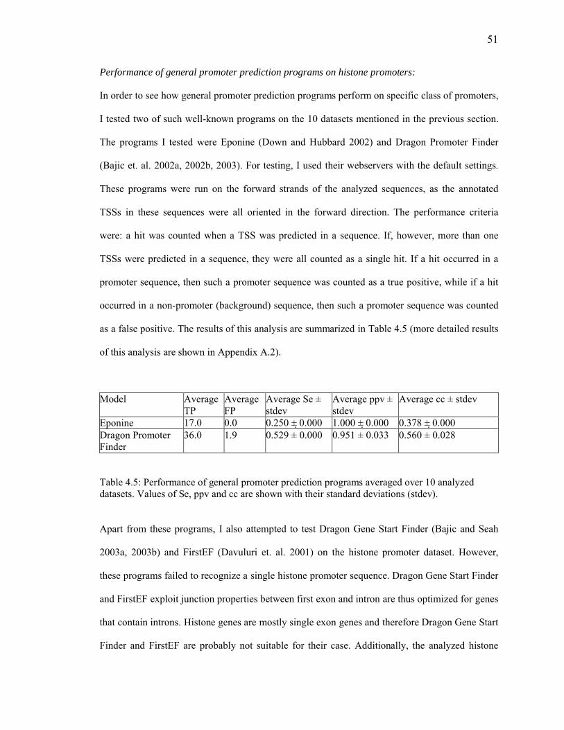
51

Performance of general promoter prediction programs on histone promoters:

In order to see how general promoter prediction programs perform on specific class of promoters,

I tested two of such well-known programs on the 10 datasets mentioned in the previous section.

The programs I tested were Eponine (Down and Hubbard 2002) and Dragon Promoter Finder

(Bajic et. al. 2002a, 2002b, 2003). For testing, I used their webservers with the default settings.

These programs were run on the forward strands of the analyzed sequences, as the annotated

TSSs in these sequences were all oriented in the forward direction. The performance criteria

were: a hit was counted when a TSS was predicted in a sequence. If, however, more than one

TSSs were predicted in a sequence, they were all counted as a single hit. If a hit occurred in a

promoter sequence, then such a promoter sequence was counted as a true positive, while if a hit

occurred in a non-promoter (background) sequence, then such a promoter sequence was counted

as a false positive. The results of this analysis are summarized in Table 4.5 (more detailed results

of this analysis are shown in Appendix A.2).

Model Average TP

Average FP

Average Se ± stdev

Average ppv ± stdev

Average cc ± stdev

Eponine 17.0 0.0 0.250 ± 0.000 1.000 ± 0.000 0.378 ± 0.000Dragon Promoter Finder

36.0 1.9 0.529 ± 0.000 0.951 ± 0.033 0.560 ± 0.028

Table 4.5: Performance of general promoter prediction programs averaged over 10 analyzed datasets. Values of Se, ppv and cc are shown with their standard deviations (stdev).

Apart from these programs, I also attempted to test Dragon Gene Start Finder (Bajic and Seah

2003a, 2003b) and FirstEF (Davuluri et. al. 2001) on the histone promoter dataset. However,

these programs failed to recognize a single histone promoter sequence. Dragon Gene Start Finder

and FirstEF exploit junction properties between first exon and intron are thus optimized for genes

that contain introns. Histone genes are mostly single exon genes and therefore Dragon Gene Start

Finder and FirstEF are probably not suitable for their case. Additionally, the analyzed histone

52

sequences did not contain full exon segments and this may also have affected the performance of

Dragon Gene Start Finder and FirstEF.

Overall, it is clear from the above analysis that the general promoter prediction programs are not

entirely suitable for predicting this specific class of promoters.

4.2.5 Human genome scan using human histone promoter structure model

The aim of this experiment was to discover regions in the human genome that have structures

similar to the structure of histone promoters. Such regions in the genome may, in part, represent

promoters of genes that have increased likelihood to be co-regulated with some of the histone

genes. It is generally expected that genes that have similar structures of regulatory regions are co-

regulated in some way.

Using UCSC Genome browser, I collected 25 human chromosomal sequences corresponding to

the human genome build, HG17. The chromosomes used for this experiment were, Chr1 through

Chr22, ChrM, ChrX and ChrY. For this analysis, I also used histone promoter structure model

M3 that gave the best overall performance as compared to the other models mentioned in the

previous section. Additionally, I used 10 PWMs and associated parameters described in section

4.2.3. For training model M3, I used the dataset on which model M3 gave the best performance

(i.e. training-data-1, refer model comparison analysis section in Appendix A.2).

Genome preprocessing

As a preprocessing step, using long sequence processing module of DPM the entire genome was

scanned with the PWM of CAAT-box. This is because CAAT-box was the most frequently

occurring TFBS in the training histone promoters (60 out of 68 histone promoters). Wherever

CAAT-box was detected on the genome, a segment [-425,+175] with respect to the motif was

53

extracted for further analysis if its GC-nucleotide content was over 37% (which was the minimum

value in training histone promoters). The segment coordinates were chosen based on the fact that

CAAT-box usually occurs around 75bp upstream of the TSS in the promoters, which means it is

located in the proximal promoter region upstream of the TATA-box (~30bp upstream of TSS)

(Bucher 1990). Biologically, CAAT-box is a commonly found promoter element that controls

temporal and spatial expression of the associated gene. The segments obtained after CAAT-box

genome scan were all separately scanned with the PWMs of the ten analyzed histone promoter

TFBSs. After PWM scanning, those segments that contained three or more motifs were short

listed and fed to the DPM system as query sequences for further analysis. The DPM system

applied the histone promoter model to the query sequences, and classified each query sequence to

one of the two predefined classes (histone promoter and non-promoter). This way, I obtained

regions on the genome that DPM predicted as histone class.

Prediction matching with RefSeq genes on the genome

Each of the genomic segment predicted by DPM as histone class was mapped back to the genome

and extended by 500 bp on either side. I then checked if any gene annotation was available for

this extended region using UCSC browser (RefSeq human gene data, build HG17, May 2004) and

Entrez Gene. The RefSeq data contained entries for 18450 unique human genes.

It can be observed from Table 4.6 that there were 1351936 CAAT-box predictions by DPM in the

initial genome scan. This large number of predictions is expected due to nonspecific model of

CAAT-box, and thus many of these are likely to be nonfunctional. Of the 1351936 query

segments analyzed around the CAAT-box motif, DPM qualified 504070 segments with three

motifs or more. Of these segments with three or more motifs, DPM predicted 134626 as histone

class. Of these, 16978 DPM predictions mapped (redundantly) with 23581 gene transcripts. Thus,

the majority of the predictions fell in the intergenic regions.

54

The 23581 gene transcripts that were mapped by DPM predictions corresponded to 6432 known

genes. There were four ways in which a prediction mapped a gene, namely, i) predicted segment

covering the TSS of the gene, ii) segment covering end of the gene transcript, iii) segment located

within the transcript, and iv) transcript located within the segment. Such positional bias of

mapping of the predicted segments with gene transcripts is shown in Table 4.7. It is evident that

most of the predictions fell within the gene loci. This suggests that there could possibly be

regulatory regions within the gene loci. Some of the genes have previously been reported with

similar features (Carninci et. al. Nature Genetics, 2006). In addition to this, there were 1334

unique genes (Appendix A.5) including most histone genes whose promoter regions, including

the TSS, were covered by the predictions. These genes may have similar promoter structure as

histone genes and therefore are expected to be co-regulated with histone genes.

Many of the DPM predictions overlapped with each other. Table 4.8 indicates the magnitude of

overlap between predictions that were classified as histone class on each chromosome. Broadly,

there were 134626 histone-class predictions that formed 84203 non-overlapping clusters.

Coexpression analysis

The 1334 genes whose promoters & TSSs were covered by the DPM predicted segments were

further analyzed by checking if they co-expressed with the histone genes. This is because

promoters are the most well annotated regulatory regions on the human genome and can generally

be correlated with their associated genes’ co-expression data. Also, there are no data yet available

on genes co-regulated with histone genes which I could possibly have used directly to validate

my results. For this co-expression analysis, I used UCSC Genome browser’s Gene Sorter utility

(with human GNF Gene Expression Atlas2 data, which are based on U133A and GNF1H

Affymetrix chips). Gene Sorter returns a ranked list of at most 1000 genes based on the similarity

55

of the expression of each gene to the query gene. This way, I collected all co-expressed genes

returned by Gene Sorter for each of the 68 histone genes analyzed. Gene Sorter did not have entry

for three histone genes (Ids: 8338, 85235, 255626) so these were not considered, while the entry

for gene with ID:83740 showed co-expression data for Gene ID:474382 (another histone gene not

part of training data). The histone gene co-expression data collected from Gene Sorter is shown

here (http://research.i2r.a-star.edu.sg/DPM/CAAT_Genome_Scan/Histone_coexpression.txt). The

data contained expression information on 6052 unique genes.

Of 1334 genes predicted to be co-regulated (with similar promoter structure) with histone genes,

517 genes (Appendix A.5) were found to be co-expressed with the histone genes by validating

their presence in the Gene Sorter histone gene co-expression data collected from Gene Sorter.

p-value analysis

Using hypergeometric distribution, I calculated p-value for the coexpression results using the

formula: C(K,k)C(N-K,n-k)/C(N,n), where

N = # of cases in the total population,

n = # of cases in a selected subpopulation of N,

K = # of cases in the total population that has a specific characteristics,

k = # of cases in the subpopulation that has the specific characteristics,

C(x,y) = the number of ways to choose y items from a bag of x items, without replacement.

Applying the above to the present problem, we get,

N=18450 (Total number of unique genes known - RefSeq data)

n=1334 (Of 18450 known genes, 1334 genes have promoters similar to histone promoters)

K=6052 (Of 18450 known genes, 6052 genes coexpress with histone genes)

k=517 (Of 1334 genes that have promoters similar to histone promoters, 517 genes coexpress

with histone genes).

56

This gives us a p-value = 1.173e-006 and corrected p-value = 0.0216 (using correction factor of

18450 for multiplicity testing), which suggests that the results obtained are statistically significant

at cutoff p-value of 0.05.

Detection of histone genes

In this genome scan analysis DPM successfully identified 62 histone promoters from across the

genome that contained the CAAT-box. Of these, 53 histone promoters were part of the training

data, while the remaining nine were not. Thus, DPM was able to recognize a large number of

training histone sequences that contained CAAT-box (53 out of 60). Interestingly, DPM was also

able to detect nine histone promoters that were not part of the training data (refer result here

http://research.i2r.a-

star.edu.sg/DPM/CAAT_Genome_Scan/histone_gene_recognition_analysis.xls). Of the total 62

histone genes detected, all but one (GeneID: 9555) had their promoter regions along with their

TSSs covered by the predictions.

Distribution of predictions on probability scale

In order to see how the frequency of all histone class DPM predictions (i.e. predictions with

probability > 0.5) behaved against probability scale, I divided the prediction probability range

between 0.5 and 1 into five equal bins and calculated the frequency of predictions in each bin.

The same procedure was repeated separately for, i) predictions that mapped with known genes, ii)

predictions in i) that covered the TSS of the genes, iii) predictions in ii) that were found to be co-

expressed with histone genes. These four distributions are shown in Table 4.9. It can be observed

that in all four cases highest number of predictions and the genes mapped lie above probability of

0.9. Broadly, number of predictions and mapped genes followed similar increasing trend against

probability value. Of 134626 total predictions, 46093 predictions (34.2%) fell in the range above

0.9. Similarly, of 16978 predictions that mapped with known genes 5417 (31.9%) predictions fell

57

in the highest probability range; of 2107 predictions that mapped the TSS of the known genes 953

(45.2%) fell in the highest probability range; of 856 predictions that mapped TSS of the genes

that were found to co-express with histone genes 417 (48.7%) fell in the highest probability

range. Thus, we see that the percentage of the total among these four categories in the probability

range > 0.9 was highest for the co-expressed gene category. This is expected as co-expressed

genes are expected to be functionally related with histone genes and thus are likely to also be co-

regulated and have similar promoter structures as histone promoters. Due to this promoter

structure similarity, bulk of the co-expressed gene predictions is classified by DPM in the highest

probability range.

A closer examination of the range above 0.9 also revealed that a large majority of predictions that

mapped with histone genes were present in this range. In all, 56 histone gene promoters were

detected (refer Appendix A.6 for detected genes) in this range compared to a total of 62 histone

gene promoters that were predicted in the entire range between 0.5 and 1. This is expected

because predictions that map with histone gene promoters should closely match with the DPM

histone promoter model and thus should generally be assigned higher probabilities.

Biological-terms analysis

I performed functional biological annotations on the 1334 predicted histone co-regulated genes

(refer Table 4.9) in order see how they were related among themselves. I used DAVID 2.1

(Dennis et. al. 2003; see also http://david.abcc.ncifcrf.gov/summary.jsp) for this purpose. Fig 4.5

is a screenshot of DAVID output which shows biologically important terms in the decreasing

order of statistical significance. Below are some of the terms associated with predicted histone

co-regulated genes in various functional categories (numbers in brackets represent number of

genes the term is associated with):

58

- Top three most statistically significant terms: Nuclear protein (355), dna-binding (203) and

intracellular membrane-bound organelle (531)

- Top three most frequent SP_PIR_KEYWORDS terms: nuclear protein (355), alternative

splicing (218), dna-binding (203)

- Top three most frequent gene ontology (GO) molecular function (MF) terms: binding (761),

nucleic acid binding (340), protein binding (332).

- Top three most frequent GO biological process (BP) terms: cellular process (814), physiological

process (785), cellular physiological process (739).

- Top three most frequent GO cellular component (CC) terms: cell (788), intracellular (669) and

organelle (592).

Overall, it appears that a large number of our predicted genes share many biological terms among

themselves. Many of these terms are also associated with histone genes, indicating that these

predicted genes with similar promoter structures may also have function related to histone genes.

There appears a correlation between promoter similarity and biological terms.

No predictions on Chromosome M

From Table 4.6, it can be observed that there are no DPM predictions on Chromosome M. This

suggests that mitochondrial genome does not contain any genes that are possibly co-regulated

with histone genes and have similar function. This is in line with what is biologically known that

mitochondrial genome is free of histones (Jansen 2000) and does not pack into chromatin. This is

in contrast to nuclear chromosomes that pack into chromatin with the help of histones.

Additionally, Chromosome M is present in the cytoplasm and not in the nucleus like nuclear

chromosomes. All genes in Chromosome M are present on a single circular DNA molecule.

Genes on Chromosome M are also different from genes on nuclear chromosomes in that, i)

different genes on Chromosome M may share the same coding bases and ii) some codons don’t

59

Fig 4.5: Screenshot of DAVID showing biological terms shared by 1334 DPM predicted histone co-regulated genes.

follow universal translation rules. Overall, it appears that genes on Chromosome M follow

different regulatory mechanism compared to nuclear genes.

This example demonstrates that DPM behaves according to our expectations, i.e. it recognizes a

large proportion of the target promoter group (histones) and also recognizes other regulatory

regions, including promoters, with similar structure as histone promoter model. The recognized

promoters may possibly correspond to the genes that are co-regulated with histone genes. I could

not validate these histone coregulated genes with any experimental data as this information is not

60

yet known. Instead, I validated the results with microarray based histone gene expression data on

the premise that co-expressed genes are also co-regulated though this may not be true always.

From the results it appears that a large number of genes are possibly co-regulated and also co-

expressed with the histone genes. This may be true, as histone genes are known to have a

widespread expression in tissues both in developmental and differentiated cell-lines (Doenecke et.

al. 1997, Osley 1991). This widespread expression pattern of histone genes may be due to the fact

that histone proteins play a critical role in chromosomal processes such as gene transcription,

regulation, chromosome condensation, recombination and replication (Doenecke et. al. 1997). It

generally is not possible to pass judgment for predictions that fall in the intergenic and intragenic

regions. Apart from being possible false cases, these regions may in part represent regulatory

regions (such as promoters, enhancers, silencers and others) associated with genes that are both

known and that are possibly yet to be discovered.

Overall, this analysis has resulted in a dataset of potential genomic regulatory regions that are

similar in structure to the histone promoter structure model. However, further investigations

especially of experimental nature are warranted in this direction. This is precisely we plan to

pursue as a next logical step by collaborating with biologists working in similar fields.

61

DPM predictions DPM predictions mapped with annotated RefSeq genes (including histone genes)

Chromosome

# Predictions with CAAT-box

(A)

# (A) with motifs => 3

(B)

# (B) predicted as histone class

(C)

# (C) mapped with known genes

# Gene transcripts mapped with (C) (redundantly)

# Unique genes mapped with (C)

1 108973 39360 10669 1627 2220 6592 109843 40786 10427 1190 1641 4503 90473 34231 8642 1009 1391 3724 78265 31004 8316 741 967 2645 82101 31490 8179 869 1355 3466 76965 29486 8007 1000 1249 3847 70615 26053 6895 1011 1440 2998 66855 25329 6543 744 953 2389 56715 20600 5542 684 945 24410 65527 24104 6534 956 1317 29311 63993 23468 6037 805 1074 32312 62499 23626 6466 800 981 34813 39684 15488 4292 396 484 13114 41734 15367 4001 530 757 20115 41196 14726 4023 482 676 19816 41963 14779 4064 641 834 24517 39083 12970 3709 645 867 30618 34174 12987 3431 359 472 11519 28738 10202 3472 681 950 35020 32508 11636 3087 420 646 14721 15138 5803 1578 214 408 8622 17620 5730 1743 315 521 128M 18 5 0 0 0 0X 74725 29971 7598 807 1344 285Y 12531 4869 1371 52 89 20Total 1351936 504070 134626 16978 23581 6432*

Table 4.6: Human genome analysis with histone promoter model using DPM (using CAAT-box for initial scan).

* Note that 6432 represents sum total of unique genes mapped per chromosome, while 6424 in Table 4.9 represents total unique genes mapped across the genome. The difference is because same genes sometimes are located on multiple chromosomes.

62

Chromosome Predictions upstream of transcripts (includes TSS)

Predictions downstream of transcripts

Predictions within the transcripts

Transcripts within the predictions

Total mapped transcripts

1 279 89 1829 23 22202 150 43 1446 2 16413 80 35 1276 0 13914 62 31 874 0 9675 120 19 1216 0 13556 126 27 1032 64 12497 134 25 1281 0 14408 84 20 849 0 9539 79 29 837 0 94510 67 23 1227 0 131711 158 39 875 2 107412 128 33 820 0 98113 41 6 437 0 48414 125 17 615 0 75715 61 15 600 0 67616 148 37 649 0 83417 171 31 664 1 86718 17 7 448 0 47219 325 100 525 0 95020 47 22 577 0 64621 43 7 356 2 40822 61 21 439 0 521M 0 0 0 0 0X 133 45 1155 11 1344Y 2 8 79 0 89

Table 4.7: Positional bias between predictions and gene transcript locations.

63

Chromosome Total histone class predictions (redundant)

Total clusters of histone class predictions (non-redundant)

1 10669 67232 10427 67173 8642 54384 8316 49635 8179 51686 8007 48057 6895 43558 6543 41599 5542 3485

10 6534 406211 6037 384312 6466 405013 4292 261214 4001 259515 4023 249916 4064 261217 3709 232618 3431 215519 3472 193620 3087 199821 1578 101222 1743 1108M 0 0X 7598 4853Y 1371 729

Total 134626 84203

Table 4.8: Overlapping/redundancy in DPM predictions that are classified as histone class.

Probability range

# DPM predictions as histone class on the entire genome (A)

# of A that mapped to known genes (B)

# of B that covered the TSS of the known genes (C)

# of C that were found to coexpress with histone genes (D)

0.90 - 1 46093 5417 (2872) 953 (613) 417 (253)

0.8 - 0.9 25144 3264 (1178) 418 (254) 154 (92)

0.7 - 0.8 21637 2742 (872) 279 (168) 110 (61)

0.6 - 0.7 19568 2589 (747) 209 (141) 95 (57)

0.5 - 0.6 22184 2966 (755) 248 (158) 80 (54)

Total 134626 16978 (6424) 2107 (1334) 856 (517)

Table 4.9: Number of DPM predictions classified as histone class in five probability bins. DPM classified a genomic segment as histone class if its prediction probability was greater than 0.5. Numbers in brackets represent unique genes mapped by the predicted genomic segments. If a single gene was mapped to multiple predictions, the gene's probability bin was considered based on the prediction with the highest probability.

64

5. CONCLUSION

The present study has resulted in successful development of DPM, a generic system aimed at

modeling promoter structures of any class of genes. The methodology, however, can principally

be applied for general purpose modeling of structures of any regulatory regions including

promoters, enhancers and silencers. I have systematically illustrated the use of DPM by taking an

example of an important class of genes, known as histone genes.

Compared to several similar programs, the study clearly demonstrates better performance of

DPM on the analyzed datasets. Apart from this, the DPM system has several advantages

compared to the existing methodologies for modeling promoter structures. These have been

highlighted below along with several new concepts that have been introduced in this study:

i) first study where the promoter structure model is not rigid; a user can implement any

type of correlations between motif features based on his background knowledge.

ii) first system to explicitly allow the user to test his model.

iii) first study where the methodology explicitly classifies a DNA segment with binding

site clusters to one of the target classes.

iv) first study where the methodology can simultaneously handle multiple target classes

of sequences.

65

v) first study to create an annotated data of histone promoters. To date there are only a

handful of datasets known to the research community for which specific promoter models

have been studied. These include the sets of i) glucocorticoid and heat-shock responsive

genes (Claverie and Sauvaget 1985), ii) globin family genes (Staden 1988), iii) muscle

specific genes (Wasserman and Fickett 1998, Klingenhoff et. al. 2002), and iv) liver

specific genes (Krivan and Wasserman 2001). This study contributes another well-

annotated dataset to the research community.

vi) first study to comprehensively model histone promoter structures computationally.

vii) first study to discover regions across the human genome that have similar structure as

human histone promoters; these regions may in part represent promoters that may

potentially be co-regulated with histone genes, or other regulatory regions that have

similar structure as histone promoters. Such annotated data set of genomic segments can

be complemented with experimental analysis, an activity that we are currently engaged

with our collaborators in Germany.

I believe that research community will find DPM a useful complement to the existing set of

promoter analysis tools.

66

REFERENCES

Albig W, Trappe R, Kardalinou E, Eick S and Doenecke D (1999) The human H2A and H2B

histone gene complement. Biol. Chem., 380(1), 7-18.

Altschul SF, Gish W, Miller W, Myers EW and Lipman DJ (1990) Basic local alignment search

tool. J. Mol. Biol. 215(3):403-410.

Bailey TL and Elkan C (1994) Fitting a mixture model by expectation maximization to

discover motifs in biopolymers. Proc Int Conf Intell Syst Mol Biol, 2:28-36.

Bailey TL and Gribskov M (1998) Combining evidence using p-values: application to sequence

homology searches. Bioinformatics, 4:48-54.

Bailey TL and Noble WS (2003) Searching for statistically significant regulatory modules.

Bioinformatics, 19 Suppl 2, II16-II25.

Bajic VB (2000) Comparing the success of different prediction software in sequence analysis: a

review. Brief Bioinform 1(3):214-228.

Bajic VB and Seah SH (2003a) Dragon Gene Start Finder identifies approximate locations of the

5' ends of genes. Nucleic Acids Res 31(13):3560-3563.

Bajic VB, Chong A, Seah SH and Brusic V (2002b) Intelligent system for vertebrate promoter

recognition. IEEE Intelligent Systems 17:64-70

Bajic VB, Seah SH (2003b) Dragon gene start finder: an advanced system for finding

approximate locations of the start of gene transcriptional units. Genome Res. 13(8):1923-1929.

Bajic VB, Tan SL, Suzuki Y, Sugano S (2004) Promoter prediction analysis on the whole human

genome. Nat. Biotechnol. 22(11):1467-1473.

Bajic VB,Seah SH, Chong A, Krishnan SPT, Koh JLY and Brusic V (2003) Computer model for

recognition of functional transcription start sites in polymerase II promoters of vertebrates. J Mol

Graphics and Modelling 21(5):323-332

67

Bajic VB,Seah SH, Chong A, Zhang G, Koh JLY and Brusic V (2002a) Dragon Promoter Finder:

recognition of vertebrate RNA polymerase II promoters. Bioinformatics 18:198-199.

Berezikov E, Guryev V, Plasterk RH and Cuppen E (2004) CONREAL: conserved regulatory

elements anchored alignment algorithm for identification of transcription factor binding sites by

phylogenetic footprinting. Genome Res. 14(1):170-178.

Berman BP, Nibu Y, Pfeiffer BD, Tomancak P, Celniker SE, Levine M, Rubin GM and Eisen

MB (2002) Exploiting transcription factor binding site clustering to identify cis-regulatory

modules involved in pattern formation in the Drosophila genome. Proc. Natl Acad. Sci. USA, 99,

757-762.

Birnbaum MJ, van Wijnen AJ, Odgren PR, Last TJ, Suske G, Stein GS and Stein, JL (1995) Sp1

trans-activation of cell cycle regulated promoters is selectively repressed by Sp3. Biochemistry,

34(50), 16503-16508.

Blanchette M and Tompa M (2002) Discovery of regulatory elements by a computational method

for phylogenetic footprinting. Genome Res. 12(5):739-748.

Blanchette M and Tompa M (2003) FootPrinter: A program designed for phylogenetic

footprinting. Nucleic Acids Res. 31(13):3840-3842.

Blanchette M, Schwikowski B and Tompa M (2002) Algorithms for phylogenetic footprinting. J

Comput Biol. 9(2):211-223.

Bucher P (1990) Weight matrix descriptions of four eukaryotic RNA polymerase II promoter

elements derived from 502 unrelated promoter sequences. J Mol Biol. 212(4):563-578.

Chickering DM, Geiger D and Heckerman D (1994) Learning Bayesian Networks is NP-Hard.

Technical Report MSR-TR-94-17, Microsoft Research, Microsoft Corporation.

Carninci P, Sandelin A, Lenhard B, Katayama S, Shimokawa K, Ponjavic J, Semple CA, Taylor

MS, Engstrom PG, Frith MC, Forrest AR, Alkema WB, Tan SL, Plessy C, Kodzius R, Ravasi T,

Kasukawa T, Fukuda S, Kanamori-Katayama M, Kitazume Y, Kawaji H, Kai C, Nakamura M,

Konno H, Nakano K, Mottagui-Tabar S, Arner P, Chesi A, Gustincich S, Persichetti F, Suzuki H,

68

Grimmond SM, Wells CA, Orlando V, Wahlestedt C, Liu ET, Harbers M, Kawai J, Bajic VB,

Hume DA and Hayashizaki Y (2006) Genome-wide analysis of mammalian promoter architecture

and evolution. Nat. Genet. 38(6):626-635.

Chen QK, Hertz GZ and Stormo GD (1995) MATRIX SEARCH 1.0: a computer program that

scans DNA sequences for transcriptional elements using a database of weight matrices. Computer

Applic Biosci 13:29-35.

Chowdhary R, Ali RA, Albig W, Doenecke D and Bajic VB (2005) Promoter modeling: the case

study of mammalian histone promoters. Bioinformatics 21(11):2623-2628.

Chowdhary R, Tan SL, Ali RA, Boerlage B, Wong L and Bajic VB (April 2006) Dragon

Promoter Mapper (DPM): a Bayesian framework for modeling promoter structures.

Bioinformatics (Epub ahead of print). PMID: 16613910.

Claverie JM and Sauvaget I (1985) Assessing the biological significance of primary structure

consensus patterns using sequence databanks. I. Heat-shock and glucocorticoid control elements

in eukaryotic promoters. Comput Appl Biosci 1(2):95-104.

Courey AJ and Tjian R (1988) Analysis of Sp1 in vivo reveals multiple transcriptional domains,

including a novel glutamine-rich activation motif. Cell 55(5):887-898.

Davuluri RV, Grosse I and Zhang MQ (2001) Computational identification of promoters and first

exons in the human genome. Nat Genet 29(4):412-417.

Dempster, A.P., Laird, N.M., and Rubin, D.B (1977) Maximum Likelihood from incomplete data

via the EM algorithm. JRSSB 39:1-38.

Dennis G Jr, Sherman BT, Hosack DA, Yang J, Gao W, Lane HC, Lempicki RA (2003) DAVID:

Database for Annotation, Visualization, and Integrated Discovery. Genome Biol. 4(5):P3. Epub

2003.

Doenecke D, Albig W, Bode C, Drabent B, Franke K, Gavenis K and Witt O (1997) Histones:

genetic diversity and tissue-specific gene expression, a review. Histochem Cell Biol 107(1):1-10.

69

Dong Y, Liu D and Skoultchi AI (1995) An unstream control region required for inducible

transcription of the mouse H1(zero) histone gene during terminal differentiation. Mol. Cell Biol.,

15(4):1889-1900.

Down TA and Hubbard TJ (2002) Computational detection and location of transcription start

sites in mammalian genomic DNA. Genome Res. 12(3):458-461.

Duncliffe KN, Rondahl ME and Wells JR (1995) A H1 histone gene-specific AC-box-related

element influences transcription from a major chicken H1 promoter. Gene 163(2):227-232.

Fickett JW and Hatzigeorgiou AG (1997) Eukaryotic promoter recognition. Genome Res. 7:861-

878.

Fiedler T and Rehmsmeier M (2006) jPREdictor: a versatile tool for the prediction of cis-

regulatory elements.

Nucleic Acids Res. 34:W546-50.

Fletcher C, Heintz N and Roeder, RG (1987) Purification and Characterization of OTF-1, a

transcription factor regulating cell cycle expression of a human histone H2b gene. Cell 51:773-

781.

Frank D, Doenecke D and Albig W (2003) Differential expression of human replacement and cell

cycle dependent H3 histone genes. Gene 312:135-143.

Frech K, Danescu-Mayer J, Werner T (1997) A novel method to develop highly specific models

for regulatory units detects a new LTR in GenBank which contains a functional promoter. J. Mol.

Biol. 270:674-687.

Freeman L, Kurumizaka H and Wolffe AP (1996) Functional domains for assembly of histones

H3 and H4 into the chromatin of Xenopus embryos. Biochemistry:Proc. Natl. Acad. Sci.

93:12780-12785.

Friedman N, Geiger D and Goldszmidt M (1997) Bayesian network classifiers. Machine Learning

29:131-163.

70

Frith MC, Hansen U and Weng Z (2001) Detection of cis-element clusters in higher eukaryotic

DNA. Bioinformatics 17(10):878-889.

Frith MC, Li MC and Weng Z (2003) Cluster-Buster: Finding dense clusters of motifs in DNA

sequences. Nucleic Acids Res. 31(13):3666-3668.

Frith MC, Spouge JL, Hansen U and Weng Z (2002) Statistical significance of clusters of motifs

represented by position specific scoring matrices in nucleotide sequences. Nucleic Acids Res.

30(14):3214-3224.

Ghosh D (1993) Status of the transcription factors database. Nucleic acids Res. 21:2091-2093.

Grundy, W.N., Bailey, T.L., Elkan, C.P., and Baker, M.E (1997) Meta-MEME: motif-based

hidden Markov models of protein families. Comput Appl Biosci. 13(4):397-406.

GuhaThakurta D and Stormo GD (2001) Identifying target sites for cooperatively binding

factors, Bioinformatics 17:608-621.

Gupta M and Liu JS (2005) De novo cis-regulatory module elicitation for eukaryotic genomes.

Proc Natl Acad Sci. 102(20):7079-7084.

Hagen G, Muller S, Beato M and Suske G (1994) Sp1-mediated transcriptional activation is

repressed by Sp3. EMBO J. 13(16):3843-3851.

Halfon MS, Grad Y, Church GM, and Michelson AM (2002) Computation-based discovery of

related transcriptional regulatory modules and motifs using an experimentally validated

combinatorial model. Genome Res. 12(7):1019-1028.

Hannenhalli S and Levy S (2001) Promoter prediction in the human genome. Bioinformatics

17(1):S90-S96.

Higgins D, Thompson J, Gibson T Thompson JD, Higgins DG and Gibson TJ (1994) CLUSTAL

W: improving the sensitivity of progressive multiple sequence alignment through sequence

weighting, position-specific gap penalties and weight matrix choice. Nucleic Acids Res. 22:4673-

4680.

71

Huang, C., and Darwiche, A (1994) Inference in Belief Networks: A Procedural Guide. Intl. J.

Approximate Reasoning, 11:1-158.

Hughes JD, Estep PW, Tavazoie S and Church GM (2000) Computational identification of cis-

regulatory elements associated with groups of functionally related genes in Saccharomyces

cerevisiae, J Mol Biol. 296:1205-1214.

Hutchinson GB (1996) The prediction of vertebrate promoter regions using differential hexamer

frequency analysis. Comput. Appl. Biosci. 12(5):391-398.

Imhof A and Becker PB (2001) Modifications of the histone N-terminal domains. Evidence for an

"epigenetic code"? Mol. Biotechnol. 17(1):1-13.

Ioshikhes IP and Zhang MQ (2000) Large-scale human promoter mapping using CpG islands.

Nat. Genet. 26(1):61-63.

Jansen RP (2000) Origin and persistence of the mitochondrial genome. Hum. Reprod. 15(2):1-10.

Jegga AG, Gupta A, Gowrisankar S, Deshmukh MA, Connolly S, Finley K and Aronow BJ

(2005) CisMols Analyzer: identification of compositionally similar cis-element clusters in

ortholog conserved regions of coordinately expressed genes. Nucleic Acids Res. 33:W408-W411.

Erratum in: Nucleic Acids Res., 2005, 33(13):4377.

Jegga AG, Sherwood SP, Carman JW, Pinski AT, Phillips JL, Pestian JP and Aronow BJ (2002)

Detection and visualization of compositionally similar cis-regulatory element clusters in

orthologous and coordinately controlled genes. Genome Res. 12:1408-1417.

Jensen FV (2001) Bayesian Networks and Decision Graphs. Springer Verlag.

Kel-Margoulis OV, Kel AE, Reuter I, Deineko IV, and Wingender E (2002) TRANSCompel: a

database on composite regulatory elements in eukaryotic genes. Nucleic Acids Res. 30:332-334.

Klingenhoff A, Frech K, Quandt K, Werner T (1999) Functional promoter modules can be

detected by formal models independent of overall nucleotide sequence similarity. Bioinformatics

15:180-186.

72

Klingenhoff A, Frech K, Werner T (2002) Regulatory modules shared within gene classes as well

as across gene classes can be detected by the same in silico. In Silico Biol 2: S17–26.

Knudsen S (1999) Promoter 2.0: for the recognition of PolII promoter sequences. Bioinformatics

15:356-361.

Kolchanov NA, Ignatieva EV, Ananko EA, Podkolodnaya OA, Stepanenko IL, Merkulova TI,

Pozdnyakov MA, Podkolodny NL, Naumochkin AN and Romashchenko AG (2002)

Transcription Regulatory Regions Database (TRRD): its status in 2002. Nucleic Acids Res.

30(1):312-317.

Krivan W and Wasserman WW (2001) A predictive model for regulatory sequences directing

liver-specific transcription. Genome Res. 11(9):1559-1566.

La Bella F and Heintz, N (1991) Histone gene transcription factor binding in extracts of normal

human cells. Mol. Cell. Biol. 11:5825-5831.

Lenhard B, Sandelin A, Mendoza L, Engstrom P, Jareborg N and Wasserman WW (2003)

Identification of conserved regulatory elements by comparative genome analysis. J. Biol. 2(2):13.

Epub 2003 May 22.

Liu X, Brutlag DL and Liu JS (2001) BioProspector: discovering conserved DNA motifs in

upstream regulatory regions of co-expressed genes. Pac. Symp. Biocomput. pp. 127-38.

Liu XS, Brutlag DL and Liu JS (2002) An algorithm for finding protein-DNA binding sites

with applications to chromatin-immunoprecipitation microarray experiments. Nat. Biotechnol.

20:835-839.

Loots GG, Ovcharenko I, Pachter L, Dubchak I and Rubin EM (2002) rVista for comparative

sequence-based discovery of functional transcription factor binding sites. Genome Res. 12:832-

839.

Luo RX and Dean DC (1999) Chromatin remodeling and transcriptional regulation. J. Natl.

Cancer Inst. 91(15):1288-1294.

73

Markstein, M, Markstein P, Markstein V and Levine MS (2002) Genomewide analysis of

clustered Dorsal binding sites identifies putative target genes in the Drosophila embryo. Proc.

Natl Acad. Sci. USA, 99:763-768.

Matis S, Xu Y, Shah M, Guan X, Einstein JR, Mural R and Uberbacher E (1996) Detection of

RNA polymerase II promoters and polyadenylation sites in human DNA sequence. Comput.

Chem. 20(1):135-140.

Matys V, Fricke E, Geffers R, Gossling E, Haubrock M, Hehl R, Hornischer K, Karas D, Kel AE,

Kel-Margoulis OV, Kloos DU, Land S, Lewicki-Potapov B, Michael H, Munch R, Reuter I,

Rotert S, Saxel H, Scheer M, Thiele S and Wingender E (2003) TRANSFAC: transcriptional

regulation, from patterns to profiles. Nucleic Acids Res. 31(1):374-378.

McCue LA, Thompson W, Carmack C, Ryan MP, Liu JS, Derbyshire V and Lawrence CE (2001)

Phylogenetic footprinting of transcription factor binding sites in proteobacterial genomes. Nucleic

Acids Res. 29(3):774-782.

McCue LA, Thompson W, Carmack CS and Lawrence CE (2002) Factors influencing the

identification of transcription factor binding sites by cross-species comparison. Genome Res.

12(10):1523-1532.

Meergans T, Albig W and Doenecke D (1998) Conserved sequence elements in human main

type-H1 histone gene promoters: their role in H1 gene expression. Eur. J. Biochem. 256(2):436-

446.

Mitra P, Xie RL, Medina R, Hovhannisyan H, Zaidi SK, Wei Y, Harper JW, Stein JL, van

Wijnen AJ and Stein GS (2003) Identification of HiNF-P, a key activator of cell cycle-controlled

histone H4 genes at the onset of S phase. Mol Cell Biol. 23(22):8110-8123.

Murphy K (2001) An introduction to graphical models. Technical report, Intel Research

Technical Report.

74

Nakajima N, Horikoshi M and Roeder, RG (1988) Factors involved in specific transcription by

mammalian RNA polymerase II: purification, genetic specificity, and TATA box-promoter

interactions of TFIID. Mol. Cell Biol. 8(10):4028-4040.

Narang V, Sung WK, and Mittal A (2005) Computational modeling of oligonucleotide positional

densities for human promoter prediction. Artif. Intell. Med. 35(1-2):107-119.

Neuwald AF, Liu JS, and Lawrence CE (1995) Gibbs motif sampling: detection of bacterial outer

membrane protein repeats Protein Sci. 4:1618-1632.

Ohler U (2006) Identification of core promoter modules in Drosophila and their application in

accurate transcription start site prediction. Nucleic Acids Res. 34(20):5943-5950.

Ohler U, Liao GC, Niemann H and Rubin GM (2002) Computational analysis of core promoters

in the Drosophila genome. Genome Biol. 3(12):RESEARCH0087. Epub 2002 Dec 20.

Osley, M.A (1991) The regulation of histone synthesis in the cell cycle. Annual Rev. Biochem.

60:827-861.

Oswald F, Dobner T and Lipp, M (1996) The E2F Transcription Factor Activates a Replication-

Dependent Human H2A Gene in Early S Phase of the Cell Cycle. Molecular and Cell Biol.

16(5):1889-1895

Pauli U, Chrysogelos S, Stein G, Stein J and Nick H (1987) Protein-DNA interactions in vivo

upstream of a cell cycle-regulated human H4 histone gene. Science 236(4806):1308-1311.

Pedersen AG, Baldi P, Chauvin Y and Brunak S (1999) The biology of eukaryotic promoter

prediction - a review. Computers and Chemistry 23:191-207.

Peretti M and Khochbin S (1997) The evolution of the differentiation-specific histone H1 gene

basal promoter. J. Mol. Evol. 44(2):128-134.

Ponger L and Mouchiroud D (2002) CpGProD: identifying CpG islands associated with

transcription start sites in large genomic mammalian sequences. Bioinformatics 18(4):631-633.

Praz V, Perier RC, Bonnard C and Bucher P (2002) The Eukaryotic Promoter Database, EPD:

new entry types and links to gene expression data. Nucleic Acids Res. 30:322-324

75

Prestridge DS (1995) Predicting Pol II promoter sequences using transcription factor binding

sites. J. Mol. Biol. 249(5):923-932.

Prestridge DS (2000) Computer software for eukaryotic promoter analysis. Review. Methods

Mol. Biol. 130:265-295.

Reese MG (2001) Application of a time-delay neural network to promoter annotation in the

Drosophila melanogaster genome. Comput. Chem. 26(1):51-56.

Sandelin A and Wasserman WW (2004) Constrained binding site diversity within families of

transcription factors enhances pattern discovery bioinformatics. J. Mol. Biol. 338(2):207-215.

Sandelin A, Alkema W, Engstrom P, Wasserman WW and Lenhard B (2004) JASPAR: an open-

access database for eukaryotic transcription factor binding profiles. Nucleic Acids Res. 32:D91-

D94.

Scherf M, Klingenhoff A and Werner T (2000) Highly specific localization of promoter regions

in large genomic sequences by PromoterInspector: a novel context analysis approach. J. Mol.

Biol. 297(3):599-606.

Schroeder MD, Pearce M, Fak J, Fan H, Unnerstall U, Emberly E, Rajewsky N, Siggia ED and

Gaul U (2004) Transcriptional control in the segmentation gene network of Drosophila. PLoS

Biol. 2(9):E271.

Segal E and Sharan R (2005) A discriminative model for identifying spatial cis-regulatory

modules. J. Comput. Biol. 12(6):822-834.

Sinha S and Tompa M (2000) A statistical method for finding transcription factor binding

sites. Proc. Int. Conf. Intell. Syst. Mol. Biol. 8:344-54.

Sinha S, van Nimwegen E and Siggia ED (2003) A probabilistic method to detect regulatory

modules. Bioinformatics 19(1): i292-i301.

Sosinsky A, Bonin CP, Mann RS and Honig B (2003) Target Explorer: An automated tool for the

identification of new target genes for a specified set of transcription factors. Nucleic Acids Res.

31(13):3589-3592.

76

Staden R (1988) Methods to define and locate patterns of motifs in sequences. Comput. Appl.

Biosci. 4(1):53-60.

Stormo GD (2000) DNA binding sites: representation and discovery. Bioinformatics 16(1):16-23.

Thompson W, Rouchka EC and Lawrence CE (2003) Gibbs Recursive Sampler: finding

transcription factor binding sites. Nucleic Acids Res. 31(13):3580-3585.

Trappe R, Doenecke D and Albig W (1999) The expression of human H2A-H2B histone gene

pairs is regulated by multiple sequence elements in their joint promoters. Biochim. Biophys.

Acta. 446(3):341-351.

Turner J and Crossley M (1999) Mammalian Kruppel-like transcription factors: more than just a

pretty finger. Trends Biochem Sci. 24(6):236-240.

van Wijnen AJ, Wright KL, Lian JB, Stein JL and Stein GS (1989) Human H4 Histone Gene

Transcription Requires the Proliferation-specific. Nuclear Factor HiNF-D. J. Biol. Chem.

264:15034-15042.

Wasserman WW and Fickett W (1998) Identification of regulatory regions which confer muscle-

specific gene expression. J. Mol. Biol. 278:167-181.

Wasserman WW, Palumbo M, Thompson W, Fickett JW and Lawrence CE (2000) Human-

mouse genome comparisons to locate regulatory sites. Nat. Genet. 26(2):225-228.

Werner T (1999) Models for prediction and recognition of eukaryotic promoters. Mammalian

Genome 10:168-175.

Werner T (2001) The promoter connection. Nat. Genet. 29(2):5-6.

Werner T (2003) The state of the art of mammalian promoter recognition. Briefings in

Bioinformatics 4(1):22-30.

Witt O, Albig W and Doenecke D (1997) Transcriptional regulation of the human replacement

histone gene H3.3B. FEBS Lett. 408(3):255-260.

Workman CT and Stormo GD (2000) ANN-Spec: a method for discovering transcription factor

binding sites with improved specificity. Pac. Symp. Biocomput. 467-78.

77

Yagi H, Kato T, Nagata T, Habu T, Nozaki M, Matsushiro A, Nishimune Y, Morita T (1995)

Regulation of the mouse histone H2A.X gene promoter by the transcription factor E2F and

CCAAT binding protein. J. Biol. Chem. 270(32):18759-18765.

Yang L, Huang E and Bajic VB (2004) Some implementation issues of heuristic methods for

motif extraction from DNA sequences. Int. J. Comp. Syst. Signals (accepted).

78

APPENDIX A:

A.1 Input and output files for the DPM system

Following are the input files required by DPM. These are either intermediate files created by the

system or are user provided. The sample files shown below for training data, PWM, HOMD

training data, and model definition were used in the analysis of modeling promoter structure of

human histone genes.

User input files:

i) Training data: This file contains fasta DNA sequences that DPM converts to their

HOMDs prior to using them for training the Bayesian model. These sequences may belong to two

or more classes. For example, if there is one promoter class that a user wishes to model, then the

other class may represent background (non-promoter) sequences. The class categorization and the

number of classes to consider for analysis, however, depend on the modeling objectives. The

sequences in the training data must all be of the same length. Note that the Class information

should be present as the first field in the header of the fasta sequences, the format of which looks

like:

>Class_name|any description about the sequenceacttttttaagggggaaa...Note that Class_name must not start with a numeric character.

Sample training data file: http://research.i2r.a-star.edu.sg/DPM/Training_data.txt

ii) Query data: This file contains fasta DNA sequences that DPM converts to their

HOMDs prior predicting regions in them that match well with a trained Bayesian model. The

query sequences may be of arbitrary length. If the query sequences are long, they are first

processed with long sequence processing module (described below). Note that the query

sequences do not contain the Class information in their headers.

79

Sample query data file: http://research.i2r.a-star.edu.sg/DPM/Query_data.txt

iii) PWM: A PWM file contains PWMs of motifs that are believed to be present in the

analyzed promoter sequences. PWMs are commonly used probabilistic models for representing

TFBSs. PWMs are generally obtained from resources such as, TRANSFAC, JASPAR, biological

literature and ab-initio motif discovery techniques. A PWM may conceptually contain a core

region that corresponds to the most conserved portion of the PWM. In contrast, the matrix region

of the PWM corresponds to the entire PWM matrix. PWMs are commonly used to discover

motifs in a genomic sequence. The sequence is scanned with a PWM and the motifs that meet

some threshold criteria are reported back. In order to illustrate the PWM file format used by

DPM, I take the example of PWM for TATA-box (taken from Bucher 1990):

TATA -> Name of the TFBSCols: 15 -> Total number of columns in the PWM to represents a TFBSCoreStart: 2 CoreEnd: 7 -> CoreStart and CoreEnd represent the boundaries of the core region of the PWM. The core region of the PWM represents biologically known consensus of the TFBS and is the most conserved part of the PWM matrix. For example, PWM core region for TATA-box is "TATAAA" and represents columns 2 through 7 in the PWM matrix shown below.CoreCutoff: 0.90 MatrixCutoff: 0.85 -> CoreCutoff is the cut-off score for the core region, while MatrixCutoff is the cut-off score for the matrix region. Motifs with core and matrix region scores above their respective user-defined cutoff values are considered for reporting. These scores may range between 0 and 1.Strand: 1 -> Which strand to scan, 1 for positive strand, while 2 for both strandsTop: 1 -> Number of motifs desired in the output. This parameter limits the number of motifs reported back. For example, if "Top" is set to 1, and two motifs qualify the cutoff, then the one with the higher core score is selected, and if the core scores are equal in both cases then the one with the higher matrix score is selected. If for two motifs core scores are the same, while the matrix scores are also the same, the first identified motif is selected.61 16 352 3 354 268 360 222 155 56 83 82 82 68 77 -> PWM145 46 0 10 0 0 3 2 44 135 147 127 118 107 101152 18 2 2 5 0 10 44 157 150 128 128 128 139 14031 309 35 374 30 121 6 121 33 48 31 52 61 75 71// -> Delimiter indicating the end of one TFBS definition.

Sample PWM file: http://research.i2r.a-star.edu.sg/DPM/PWM.txt

80

Automatically generated intermediate files:

iv) HOMD training data: This file is generated by DPM by transforming the raw training

sequences to a desired HOMD format. In the file, first two lines are headers followed by the

actual data, one line corresponding to one fasta sequence in the training data. The second line of

the header defines the higher order motif features such as, motif name (Mi), strand (Si) and

mutual spacer length between adjacent motifs (L(i+1)_I), for each motif position i = 1, 2...n,

where i is counted from the rightmost end of a sequence, and n is the total number of motif

positions. The total number of motif positions is automatically determined by DPM by counting

the maximum number of motifs any sequence has in the training data. For example, in the sample

HOMD training data file shown below there are eight motif positions. Missing values in the data

are considered missing at random and are denoted by a "*".

Sample HOMD training data file: http://research.i2r.a-star.edu.sg/DPM/HOMD_training_data.txt

v) HOMD Query data: This file is generated by DPM by transforming raw query

sequences to their desired HOMD format. The format of HOMD query data is the same

as HOMD training data. Since, the class for the query sequences is unknown it is denoted by a

"*" in the file.

Sample HOMD query data file: http://research.i2r.a-star.edu.sg/DPM/HOMD_query_data.txt

vi) Model definition: A model definition file basically contains the skeleton of the

Bayesian network model. Each node in the Bayesian model, as defined in the model definition

file, corresponds to a column in the HOMD training and HOMD query data. The number of

columns in the HOMD training and HOMD query data may sometimes be more than the number

of nodes defined in the model definition file. In such cases, however, columns which do not have

any node entry in the model definition file are not considered in the modeling. The order of

81

columns in HOMD training and HOMD query data files is not important. The node/column

names are case sensitive. As a utility, DPM automatically generates a sample model definition

file with a default Naive Bayes model. The user may use this default model definition as a

template to define his model; use the default Naive Bayes model or modify it if required. DPM

also provides a leave-one-out cross validation utility for the user to test his model. DPM thus

provides flexibility to the user to build and test his model before using it further. The model

definition file essentially contains four blocks of parameters delimited by single blank lines (refer

the sample model definition file below).

First Block: This block represents the symbols of Bayesian network nodes. Each line has

a node name followed by the number of states/values the node can have. For example in the

sample model definition file, the Class node represents the class of the sequences while 2

represents the total number of classes (refer sample HOMD training data). Similarly, the M nodes

(M1, M2 and others), S nodes (S1, S2 and others), and L nodes (L2_1, L3_2 and others) are

presented along with the number of states/values they can assume. For example, M and S nodes

which represent motif and strand, respectively, can assume 10 and 2 state values. M and S are

discrete nodes. The L node, which represents mutual spacer length between motifs, is discretized

to user-defined levels and is denoted by 0 against it.

Second Block: This block contains all state values for the discrete nodes M, S, and Class.

For example, all M nodes may take values from the analyzed TFBS names such as, TATA, CAAT,

GC, E2F, ATFCREB, Oct1, AC, TG, H4TF2, and RT1. The S nodes may take values of plus and

minus. Similarly, the Class node can assume values as, Histone and NonPromoter. Note that node

values should not start with a numeric character.

82

Third Block: This block is used to discretize the node L which represents the mutual

spacer length between motifs. The first line represents the number of states one wants to

discretize node L in. This is followed by the discretization levels of L. In the sample model

definition file below, there are 12 levels that demarcate 11 states of L. For example 0th level is at

0, 1st level is at 10, and so on. The INFINITY_ns level represents an infinite number. If the user

wishes to exclude the node (L) from his model, make sure to remove all the rows from the model

definition file that contains L. Also, in such a case replace the entire third block by a 0.

Fourth block: This block defines the DAG structure of the Bayesian network model. The

DAG structure gives an intuitive picture as to what dependency relationship exists between the

nodes. The DAG structure shown in the sample model definition file represents a Naive Bayes

model, which means that the Class node determines all other nodes, or all other nodes are

independent of each other given the class node. Notation for example, Class->M1, means Class

node determines node M1.

Sample model definition file: http://research.i2r.a-star.edu.sg/DPM/Model_definition.txt

Output file:

For each query sequence, DPM model outputs a probability distribution of the query sequence

over all the target sequence classes. The query sequence is then assigned by the model to the

target class with the highest probability. In other words this also means that of all the target

sequence classes, the class that gets the highest probability is closest to the input sequence in

terms of structure similarity.

Sample output file: http://research.i2r.a-star.edu.sg/DPM/DPM_output.txt

83

A.2 Model comparison analysis

Detailed results and datasets of comparative analysis of DPM histone promoter structure models

with several other programs: http://research.i2r.a-star.edu.sg/DPM/comparison/

A.3 Files related to human genome analysis using histone promoter model

Analysis files related to genome scan using initial motif scan of CAAT-box: http://research.i2r.a-

star.edu.sg/DPM/CAAT_Genome_Scan

A.4 How the long sequence processing module works?

This module of DPM is used when the query genomic sequence is long (1000s of bp long). This

module first identifies the locations of the putative binding sites on the query sequence based on a

single PWM selected by the user. The selected PWM may represent a biologically significant

motif that is over-represented in the target promoter class. The module then extracts the segments

surrounding the predicted motifs based on the user specified parameters. These parameters

include, GC-cutoff for the chosen segment (maximum being 1), length of the region upstream of

the motif, length of the region downstream of the motif, and minimum length between motifs (if

on a strand the mutual spacer length between two detected motifs is < minimum length between

motifs, the best scoring motif of them is selected for segment extraction). Minimum length

between motifs can take values greater than or equal to 0; a value of -1 returns all detected motifs.

It is recommended that the extracted segments should normally be of the same length as training

sequences. Note that long sequence processing may sometimes generate sequences shorter than

the requested range because in such cases motifs might occur near the edges of the long sequence.

The sequences are scanned on both the strands and the extracted sequences are presented from 5'

to 3'. Note that for PWM scanning by this module, strand and top parameters mentioned in the

84

PWM file are not considered. The extracted sequences are then further processed by DPM to

obtain their HOMDs.

A.5 Predicted histone co-regulated/co-expressed genes.

Following 1334 Gene IDs correspond to unique genes whose TSS and promoters were covered by DPM predictions:

24 38 47 56 60 87 118 160 185 204 259 284 293 333 369 384 394 409 421 439 468 472 506 516 526 537 546 574 640 687 801 805 811 847 875 891 899 960 972 987 989 990 991 995 999 1012 1017 1028 1069 1070 1119 1149 1152 1153 1158 1161 1163 1164 1184 1280 1288 1349 1386 1408 1415 1456 1491 1503 1514 1523 1540 1605 1621 1649 1716 1717 1730 1748 1750 1785 1837 1869 1871 1912 1973 1983 1993 1994 1996 2001 2002 2010 2020 2035 2036 2068 2069 2107 2110 2118 2145 2146 2150 2185 2222 2253 2302 2316 2335 2358 2535 2569 2620 2629 2639 2651 2665 2703 2744 2752 2768 2781 2794 2804 2829 2847 2870 2879 2896 2919 2997 3006 3007 3008 3009 3010 3012 3013 3014 3017 3018 3021 3024 3028 3047 3048 3050 3104 3110 3122 3142 3146 3148 3149 3151 3178 3182 3183 3188 3190 3191 3209 3213 3239 3274 3276 3290 3304 3305 3309 3321 3350 3376 3421 3460 3516 3550 3569 3608 3642 3670 3709 3725 3726 3727 3728 3748 3775 3781 3815 3837 3840 3843 3886 3925 3930 3998 4023 4060 4074 4077 4084 4091 4108 4170 4172 4174 4176 4200 4204 4292 4329 4361 4439 4507 4548 4595 4597 4638 4643 4698 4700 4728 4735 4758 4775 4776 4793 4800 4807 4808 4809 4824 4841 4849 4856 4891 4901 4904 4925 4926 4946 4999 5007 5008 5015 5034 5037 5075 5077 5078 5080 5096 5127 5147 5165 5187 5193 5226 5241 5271 5274 5277 5290 5300 5324 5372 5383 5395 5436 5438 5454 5495 5514 5518 5525 5528 5545 5586 5686 5691 5702 5737 5757 5775 5828 5874 5902 5926 5933 5965 5971 5980 5990 5997 6009 6046 6048 6120 6142 6175 6187 6228 6238 6241 6272 6284 6299 6302 6303 6319 6349 6351 6421 6427 6428 6431 6447 6457 6503 6513 6555 6569 6605 6626 6633 6636 6651 6658 6662 6667 6722 6723 6726 6748 6776 6790 6794 6795 6811 6818 6821 6874 6895 6975 7008 7013 7025 7041 7052 7058 7071 7141 7184 7186 7259 7260 7272 7278 7289 7297 7342 7351 7353 7405 7411 7415 7453 7472 7514 7534 7536 7547 7562 7568 7589 7620 7626 7634 7639 7678 7697 7700 7726 7737 7748 7750 7763 7779 7799 7832 7846 7857 7965 8045 8106 8241 8290 8318 8320 8329 8330 8331 8332 8334 8335 8336 8337 8338 8339 8340 8341 8342 8343 8345 8346 8347 8348 8349 8350 8351 8352 8353 8355 8356 8357 8358 8359 8364 8368 8452 8467 8490 8502 8528 8650 8655 8704 8767 8804 8854 8863 8904 8943 8968 8969 8970 8975 8989 8999 9015 9019 9020 9044 9049 9055 9101 9131 9133 9146 9149 9212 9221 9230 9232 9252 9253 9325 9361 9371 9410 9464 9467 9481 9513 9521 9560 9564 9583 9601 9612 9616 9639 9645 9653 9662 9678 9682 9688 9702 9709 9715 9730 9741 9750 9751 9759 9768 9791 9793 9810 9813 9824 9855 9862 9867 9873 9886 9887 9943 9953 9993 10001 10023 10072 10092 10105 10124 10130 10131 10146 10156 10162 10163 10171 10202 10212 10214 10220 10221 10237 10238 10245 10263 10281 10289 10298 10300 10308 10311 10362 10369 10383 10420 10424 10440 10452 10459 10469 10481 10507 10525 10600 10608 10635 10658 10668 10726 10734 10738 10793 10806 10808 10810 10844 10897 10906 10912 10938 10943 10947 10956 10957 10960 10962 10963 10989 10998 11016 11068 11153 11161 11180 11182 11194 11215 11252 11259 11273 11334 11335 11339 11346 22795 22838 22847 22850 22879 22894 22897 22903 22916 22929 22933 22936 22994 23014 23030 23093 23094 23112 23130 23142 23149 23155 23193 23243 23261 23299 23301 23324 23344 23360 23397 23404 23406 23417 23462 23468 23480 23493 23523 23559 23594 23597 23635 23660 23673 23710 24138 24139 25777 25801 25822 25824 25851 25888 25901 25921 25934 25942 25994 25998 26019 26037 26064 26137 26145 26189 26261 26330 26586 26959 27072 27109 27154 27164 27235 27250 27333 27351 27434 28955 29028 29035 29086 29098 29102 29107 29123 29841 29902 29907 29944 29946 29959 29968 29985 29990 30010 30012 30819 30834 30844 49854 50512 50814 50945 51003 51050 51078 51084 51105 51114 51119 51142 51144 51150 51155 51181 51188 51203 51218 51255 51258 51259 51295 51313 51347 51361 51362 51366 51372 51412 51427 51430 51451 51514 51538 51540 51585 51603 51605 51621 51633 51741 51742 51754 53373 53916 54441 54509 54516 54537 54545 54555 54556 54567 54586 54602 54622 54677 54704 54785 54793 54820 54830 54845 54851 54868 54873 54879 54882 54897 54904 54920 54934 54935 54943 54955 54958 54962 54969 54973 54976 55007 55032

85

55076 55106 55124 55147 55154 55156 55159 55163 55165 55166 55253 55272 55277 55278 55282 55289 55291 55322 55329 55388 55501 55502 55510 55526 55572 55676 55702 55719 55723 55737 55751 55763 55766 55771 55776 55784 55787 55794 55821 55839 55840 55858 55889 55897 55930 55973 56001 56097 56098 56104 56105 56144 56159 56242 56267 56624 56882 56910 56922 56980 56997 57102 57149 57151 57184 57185 57464 57474 57506 57547 57575 57592 57639 57659 57693 57697 57716 57795 57799 57804 57822 58492 58515 59335 60509 60672 63922 63946 63948 64288 64344 64388 64398 64598 64710 64714 64777 64782 64795 64800 64843 64850 64975 65055 65057 65068 65083 65117 65263 65983 65988 78991 79007 79008 79009 79016 79017 79018 79019 79038 79039 79084 79086 79087 79102 79152 79165 79171 79174 79622 79624 79629 79641 79672 79682 79698 79720 79733 79744 79770 79794 79805 79848 79862 79867 79873 79877 79884 79940 79955 79973 80011 80032 80099 80185 80196 80205 80207 80217 80218 80222 80264 80274 80321 80727 80765 80772 80790 80824 81551 81558 81562 81569 81576 81610 81669 81689 81788 81850 81889 81928 81931 83401 83461 83463 83473 83592 83642 83697 83698 83740 83743 83746 84060 84172 84181 84188 84193 84206 84220 84222 84223 84229 84247 84254 84266 84268 84269 84272 84275 84279 84280 84303 84309 84312 84366 84461 84504 84527 84570 84612 84676 84681 84698 84717 84722 84734 84790 84856 84872 84876 84901 84919 84954 84964 84969 85235 85236 85316 85317 85318 85319 85416 89782 89839 89953 90139 90204 90379 90592 90861 90864 91181 91433 91543 91544 91689 91750 91942 92106 92259 92291 92591 92799 92815 92906 93058 93185 93474 93622 94039 94103 112464 112495 112714 112840 113115 113246 113451 113457 113835 114034 114043 114088 114335 114336 114789 114883 114984 115362 115509 115572 115648 115703 115827 116115 116143 116254 116328 116448 116840 117178 119391 119392 119678 120103 120237 121512 122416 122525 122773 122961 123096 124044 124411 124935 124997 125061 125113 125144 125919 125950 125965 125972 126068 126074 126231 126295 126308 126792 126961 127262 127281 127700 127833 128061 128312 129025 129531 130026 130576 130940 131578 132243 133686 134429 134492 137735 138241 139285 139562 139596 140739 142689 143684 145258 145645 146279 146330 146542 146562 147138 147183 147719 147808 147841 147965 148137 148206 148213 148254 148523 148898 149465 150274 150280 150468 151651 151871 152579 152687 153571 157313 157570 157697 158248 158947 159090 159296 161829 161835 162427 163049 163227 166012 166379 166979 167691 168374 168455 170959 170960 171392 171484 171546 195828 196294 196996 199692 199745 199777 200081 200523 200634 200844 201799 202299 202559 202865 203245 203523 205327 219541 219654 219743 219938 221443 221458 221504 221613 221656 222194 222234 252839 253260 253980 254122 254863 255403 255426 255626 255919 257068 257106 259289 259290 280658 283150 283537 283768 283991 284161 284274 284359 284390 284439 284443 284459 284525 284618 284695 285074 285172 285331 285335 285349 285605 286205 317701 317749 317772 337966 338339 338785 339175 339324 339403 339476 339487 339500 339942 340061 340252 340542 340562 340602 340665 341568 342096 343169 348235 353088 353288 373863 374393 374395 374650 375346 375513 376497 386684 387103 387882 388372 388524 388531 388815 389541 389898 390061 390535 394261 399512 399717 399833 400073 400360 400673 400932 400943 401409 401898 404734 414062 414149 425054 439940 439985 440053 440072 440073 440138 440295 440321 440686 440689 440944 441178 441242 441549 442578 442582 445329 449003 474381 474382 494115 494188 494514 548593 553115 619189 642280 643549 645078 650767 664701

Of 1334 genes above, following 517 genes were found to coexpress with histone genes:

24 56 60 118 160 204 293 369 384 468 506 516 960 987 1017 1153 1161 1163 1184 1280 1386 1415 1503 1523 1649 1730 1748 1785 1869 1871 1912 1973 1983 1994 2002 2010 2035 2222 2302 2569 2629 2639 2665 2703 2768 2794 2804 2829 2870 2997 3006 3007 3008 3009 3010 3012 3014 3017 3018 3021 3024 3028 3146 3149 3151 3178 3182 3183 3190 3213 3276 3309 3376 3421 3460 3516 3608 3670 3709 3727 3998 4170 4172 4176 4200 4292 4548 4595 4700 4728 4735 4775 4808 4809 4824 4841 4849 4901 4904 4926 4946 5007 5008 5015 5034 5078 5096 5165 5193 5277 5436 5514 5525 5528 5686 5691 5757 5828 5902 6046 6142 6175 6187 6228 6302 6303 6421 6427 6428 6431 6503 6513 6555 6626 6633 6636 6651 6723 6726 6748 6776 6794 6795 6811 6818 6874 6895 6975 7071 7289 7342 7353 7415 7453 7514 7536 7568 7589 7626 7639 7726 7737 7748 7799 7965 8045 8106 8290 8329 8330 8331 8332 8334 8335 8336 8337 8339 8340 8342 8343 8345 8346 8347 8348 8349 8350 8351 8352 8353 8355 8356 8357 8358 8359

86

8364 8368 8452 8968 8969 8970 8989 8999 9020 9044 9049 9131 9146 9221 9232 9252 9253 9325 9361 9371 9410 9464 9521 9583 9601 9616 9662 9682 9709 9741 9768 9791 9793 9810 9813 9855 9862 9887 9943 9953 9993 10001 10023 10092 10130 10131 10146 10156 10162 10163 10171 10212 10220 10237 10245 10263 10281 10289 10298 10362 10420 10424 10440 10452 10459 10481 10600 10608 10658 10668 10726 10738 10793 10844 10897 10943 10956 10957 10960 10989 11016 11068 11153 11180 11252 11273 22838 22847 23014 23030 23093 23130 23155 23193 23360 23480 23559 23673 25777 25801 25822 25824 25901 25921 26959 27154 27164 27333 27434 29086 29098 29102 29107 29841 29907 29946 30010 30844 50814 51003 51050 51078 51084 51142 51144 51150 51188 51347 51362 51372 51430 51540 51585 51603 51605 51741 51742 54509 54516 54545 54556 54586 54677 54785 54793 54820 54851 54868 54897 54904 54973 55007 55124 55147 55163 55253 55272 55277 55278 55289 55291 55702 55719 55751 55766 55771 55776 55784 55787 55794 55858 55930 56159 56242 56910 56922 56980 57102 57149 57151 57184 57592 57639 57693 57799 57822 60672 64598 64710 64777 64800 65083 65117 65988 79017 79039 79084 79086 79087 79171 79622 79672 79770 79794 79862 79873 80032 80099 80185 80196 80217 80218 80222 80264 81558 81562 81569 81610 81788 81931 83463 83592 83642 83743 83746 84172 84193 84247 84268 84269 84309 84461 84527 84570 84681 84717 84734 84790 84856 84901 84919 85236 85416 89782 89953 90592 91181 92259 92815 92906 93058 93622 112495 112840 113246 113451 114883 116143 116254 120103 122416 124044 125061 125919 125950 125972 126074 126231 126961 127700 128061 128312 129025 129531 131578 132243 137735 140739 145258 147808 147841 147965 148254 150274 151871 152579 153571 158947 161835 162427 166379 166979 168455 171392 171546 196294 196996 200523 202299 202865 203523 219541 219743 221613 222194 253260 257106 283150 284161 284439 286205 317701 317749 317772 338339 340061 340252 374395 376497 388524 389898 401409 474382

A.6 Histone gene prediction at probability > 0.9.

At probability > 0.9, genes with following Ids were rejected: 8341 8359 8364 9555 92815

132243. These six genes were mapped by 18 DPM predictions.

At probability > 0.9, genes with following Ids were accepted: 3006 3007 3008 3009 3010 3012

3013 3014 3017 3018 3021 3024 8290 8329 8330 8331 8332 8334 8335 8336 8337 8338 8339

8340 8342 8343 8345 8346 8347 8348 8349 8350 8351 8352 8353 8355 8356 8357 8358 8368

8968 8969 8970 55766 83740 85235 85236 126961 128312 221613 255626 317772 440686

440689 449003 474381 474382. These 57 genes were mapped by 97 DPM predictions. Thus,

there was a marginal loss of 6 histone genes by increasing the cutoff from 0.5 to 0.90