Embed Size (px)
Citation preview

Journal of Machine Learning Research 18 (2017) 1-37 Submitted 1/16; Revised 2/17; Published 8/17
A Bayesian Framework for Learning Rule Sets for InterpretableClassification
Tong Wang [email protected] University of Iowa
Cynthia Rudin [email protected] Duke University
Finale Doshi-Velez [email protected] Harvard University
Yimin Liu [email protected] Edward Jones
Erica Klampfl [email protected] Ford Motor Company
Perry MacNeille [email protected] Ford Motor Company
Editor: Maya Gupta
AbstractWe present a machine learning algorithm for building classifiers that are comprised of a small num-ber of short rules. These are restricted disjunctive normal form models. An example of a classifierof this form is as follows: If X satisfies (condition A AND condition B) OR (condition C) OR· · · , then Y = 1. Models of this form have the advantage of being interpretable to human expertssince they produce a set of rules that concisely describe a specific class. We present two proba-bilistic models with prior parameters that the user can set to encourage the model to have a desiredsize and shape, to conform with a domain-specific definition of interpretability. We provide a scal-able MAP inference approach and develop theoretical bounds to reduce computation by iterativelypruning the search space. We apply our method (Bayesian Rule Sets – BRS) to characterize andpredict user behavior with respect to in-vehicle context-aware personalized recommender systems.Our method has a major advantage over classical associative classification methods and decisiontrees in that it does not greedily grow the model.
Keywords: disjunctive normal form, statistical learning, data mining, association rules, inter-pretable classifier, Bayesian modeling
1. Introduction
When applying machine learning models to domains such as medical diagnosis and customer behav-ior analysis, in addition to a reliable decision, one would also like to understand how this decisionis generated, and more importantly, what the decision says about the data itself. For classificationtasks specifically, a few summarizing and descriptive rules will provide intuition about the data thatcan directly help domain experts understand the decision process.
Our goal is to construct rule set models that serve this purpose: these models provide predictionsand also descriptions of a class, which are reasons for a prediction. Here is an example of a rule setmodel for predicting whether a customer will accept a coupon for a nearby coffee house, where thecoupon is presented by their car’s mobile recommendation device:
if a customer (goes to coffee houses≥ once per month AND destination = no urgent place ANDpassenger 6= kids)
©2017 Tong Wang, Cynthia Rudin, Finale Doshi-Velez, Yimin Liu, Erica Klampfl, and Perry MacNeille.
License: CC-BY 4.0, see https://creativecommons.org/licenses/by/4.0/. Attribution requirements are provided athttp://jmlr.org/papers/v18/16-003.html.

WANG ET AL.
OR (goes to coffee houses ≥ once per month AND the time until coupon expires = one day)then
predict the customer will accept the coupon for a coffee house.
This model makes predictions and provides characteristics of the customers and their contexts thatlead to an acceptance of coupons.
Formally, a rule set model consists of a set of rules, where each rule is a conjunction of condi-tions. Rule set models predict that an observation is in the positive class when at least one of therules is satisfied. Otherwise, the observation is classified to be in the negative class. Rule set modelsthat have a small number of conditions are useful as non-black-box (interpretable) machine learn-ing models. Observations come with predictions and also reasons (e.g., this observation is positivebecause it satisfies a particular rule).
This form of model appears in various fields with various names. First, they are sparse disjunc-tive normal form (DNF) models. In operations research, there is a field called “logical analysis ofdata" (Boros et al., 2000; Crama et al., 1988), which constructs rule sets based on combinatoricsand optimization. Similar models are called “consideration sets" in marketing (see, e.g., Hauseret al., 2010), or “disjunctions of conjunctions." Consideration sets are a way for humans to handleinformation overload. When confronted with a complicated decision (such as which television topurchase), the theory of consideration sets says that humans tend to narrow down the possibilitiesof what they are willing to consider into a small disjunction of conjunctions (“only consider TV’sthat are small AND inexpensive, OR large and with a high display resolution"). In PAC learning,the goal is to learn rule set models when the data are non-noisy, meaning there exists a model withinthe class that perfectly classifies the data. The field of “rule learning" aims to construct rule setmodels. We prefer the terms “rule set" models or “sparse DNF" for this work as our goal is to createinterpretable models for non-experts, which are not necessarily consideration sets, not other formsof logical data analysis, and pertain to data sets that are potentially noisy, unlike the PAC model.
For many decisions, the space of good predictive models is often large enough to include verysimple models (Holte, 1993). This means that there may exist very sparse but accurate rule setmodels; the challenge is determining how to find them efficiently. Greedy methods used in previousworks (Malioutov and Varshney, 2013; Pollack et al., 1988; Friedman and Fisher, 1999; Gainesand Compton, 1995), where rules are added to the model one by one, do not generally producehigh-quality sparse models.
We create a Bayesian framework for constructing rule sets, which provides priors for control-ling the size and shape of a model. These methods strike a nice balance between accuracy andinterpretability through user-adjustable Bayesian prior parameters. To control interpretability, weintroduce two types of priors on rule set models, one that uses beta-binomials to model the ruleselecting process, called BRS-BetaBinomial, and one that uses Poisson distributions to model rulegeneration, called BRS-Poisson. Both can be adjusted to suit a domain-specific notion of inter-pretability; it is well-known that interpretability comes in different forms for different domains(Martens and Baesens, 2010; Martens et al., 2011; Huysmans et al., 2011; Allahyari and Lavesson,2011; Rüping, 2006; Freitas, 2014).
We provide an approximate inference method that uses association rule mining and a random-ized search algorithm (which is a form of stochastic coordinate descent or simulated annealing) tofind optimal BRS maximum a posteriori (MAP) models. This approach is motivated by a theo-retical bound that allows us to iteratively reduce the size of the computationally hard problem offinding a MAP solution. This bound states that we need only mine rules that are sufficiently fre-
2

BAYESIAN RULE SETS
quent in the database and as the search continues, the bound becomes tighter and further reduces thesearch space. This greatly reduces computational complexity and allows the problem to be solvedin practical settings. The theoretical result takes advantage of the strength of the Bayesian prior.
Our applied interest is to understand user responses to personalized advertisements that arechosen based on user characteristics, the advertisement, and the context. Such systems are calledcontext-aware recommender systems (see surveys Adomavicius and Tuzhilin, 2005, 2008; Verbertet al., 2012; Baldauf et al., 2007, and references therein). One major challenge in the design ofrecommender systems, reviewed in Verbert et al. (2012), is the interaction challenge: users typi-cally wish to know why certain recommendations were made. Our work addresses precisely thischallenge: our models provide rules in data that describe conditions for a recommendation to beaccepted.
The main contributions of our paper are as follows:
• We propose a Bayesian approach for learning rule set (DNF) classifiers. This approach in-corporates two important aspects of performance, accuracy, and interpretability, and balancebetween them via user-defined parameters. Because of the foundation in Bayesian methodol-ogy, the prior parameters are meaningful; they represent the desired size and shape of the ruleset.
• We derive bounds on the support of rules and number of rules in a MAP solution. Thesebounds are useful in practice because they safely (and drastically) reduce the solution space,improving computational efficiency. The bound on the size of a MAP model guarantees asparse solution if prior parameters are chosen to favor smaller sets of rules. More importantly,the bounds become tighter as the search proceeds, reducing the search space until the searchfinishes.
• The simulation studies demonstrate the efficiency and reliability of the search procedure.Losses in accuracy usually result from a misspecified rule representation, not generally fromproblems with optimization. Separately, using publicly available data sets, we compare ruleset models to interpretable and uninterpretable models from other popular classification meth-ods. Our results suggest that BRS models can achieve competitive performance, and areparticularly useful when data are generated from a set of underlying rules.
• We study in-vehicle mobile recommender systems. Specifically, we used Amazon Mechan-ical Turk to collect data about users interacting with a mobile recommendation system. Weused rule set models to understand and analyze consumers’ behavior and predict their re-sponse to different coupons recommended in different contexts. We were able to generateinterpretable results that can help domain experts better understand their customers.
The remainder of our paper is structured as follows. In Section 2, we discuss related work. InSection 3, we present Bayesian Rule Set modeling. In Section 4, we introduce an approximate MAPinference method using associative rule mining and randomized search. We also present theoreticalbounds on the support and the number of rules in an optimal MAP solution. In Section 5, we showthe simulation studies to justify the inference methods. We then report experimental results usingpublicly available data, including the in-vehicle recommendation system data set we created, toshow that BRS models are on-par with black-box models while under strict size restrictions for thepurpose of being interpretable.
3

WANG ET AL.
A shorter version of this work appeared at the International Conference on Data Mining (Wanget al., 2016).
2. Related Work
The models we are studying have different names in different fields: “disjunctions of conjunctions"in marketing, “classification rules" in data mining, “disjunctive normal forms" (DNF) in artificialintelligence, and “logical analysis of data" in operations research. Learning logical models of thisform has an extensive history in various settings. The LAD techniques were first applied to binarydata in (Crama et al., 1988) and were later extended to non-binary cases (Boros et al., 2000). In par-allel, Valiant (1984) showed that DNFs could be learned in polynomial time in the PAC (probablyapproximately correct - non-noisy) setting, and recent work has improved those bounds via polyno-mial threshold functions (Klivans and Servedio, 2001) and Fourier analysis (Feldman, 2012). Otherwork studies the hardness of learning DNF (Feldman, 2006). None of these theoretical approachesconsidered the practical aspects of building a sparse model with realistic noisy data.
In the meantime, the data-mining literature has developed approaches to building logical con-junctive models. Associative classification and rule learning methods (e.g., Ma et al., 1998; Liet al., 2001; Yin and Han, 2003; Chen et al., 2006; Cheng et al., 2007; McCormick et al., 2012;Rudin et al., 2013; Dong et al., 1999; Michalski, 1969; Clark and Niblett, 1989; Frank and Wit-ten, 1998) mine for frequent rules in the data and combine them in a heuristic way, where rulesare ranked by an interestingness criteria. Some of these methods, like CBA, CPAR and CMAR(Li et al., 2001; Yin and Han, 2003; Chen et al., 2006; Cheng et al., 2007) still suffer from a hugenumber of rules. Inductive logic programming (Muggleton and De Raedt, 1994) is similar, in thatit mines (potentially complicated) rules and takes the simple union of these rules as the rule set,rather than optimizing the rule set directly. This is a major disadvantage over the type of approachwe take here. Another class of approaches aims to construct rule set models by greedily adding theconjunction that explains the most of the remaining data (Malioutov and Varshney, 2013; Pollacket al., 1988; Friedman and Fisher, 1999; Gaines and Compton, 1995; Cohen, 1995). Thus, again,these methods do not directly aim to produce globally optimal conjunctive models.
There are few recent techniques that do aim to fully learn rule set models. Hauser et al. (2010);Goh and Rudin (2014) applied integer programming approaches to solving the full problems butwould face a computational challenge for even moderately sized problems. There are severalbranch-and-bound algorithms that optimize different objectives than ours (e.g., Webb, 1995). Ri-jnbeek and Kors (2010) proposed an efficient way to exhaustively search for short and accuratedecision rules. That work is different than ours in that it does not take a generative approach, andtheir global objective does not consider model complexity, meaning they do not have the same ad-vantage of reduction to a smaller problem that we have. Methods that aim to globally find decisionlists or rule lists can be used to find optimal DNF models, as long as it is possible to restrict all ofthe labels in the rule list (except the default) to the same value. A rule list where all labels exceptthe default rule are the same value is exactly a DNF formula. We are working on extending theCORELS algorithm (Angelino et al., 2017) to handle DNF.
Note that logical models are generally robust to outliers and naturally handle missing data, withno imputation needed for missing attribute values. These methods can perform comparably withtraditional convex optimization-based methods such as support vector machines or lasso (thoughlinear models are not always considered to be interpretable in many domains).
4

BAYESIAN RULE SETS
One could extend any method for DNF learning of binary classification problems to multi-class classification. A conventional way to directly extend a binary classifier is to decompose themulti-class problem into a set of two-class problems. Then for each binary classification problem,one could build a separate BRS model, e.g., by the one-against-all method. One would generatedifferent rule sets for each class. For this approach, the issue of overlapping coverage of rule setsfor different classes is handled, for instance, by an error correcting output codes (Schapire, 1997).
The main application we consider is in-vehicle context-aware recommender systems. The mostsimilar works to ours include that of Baralis et al. (2011), who present a framework that discoversrelationships between user context and services using association rules. Lee et al. (2006) create in-terpretable context-aware recommendations by using a decision tree model that considers locationcontext, personal context, environmental context and user preferences. However, they did not studysome of the most important factors we include, namely contextual information such as the user’sdestination, relative locations of services along the route, the location of the services with respectto the user’s destination, passenger(s) in the vehicle, etc. Our work is related to recommendationsystems for in-vehicle context-aware music recommendations (see Baltrunas et al., 2011; Wanget al., 2012), but whether a user will accept a music recommendation does not depend on anythinganalogous to the location of a business that the user would drive to. The setup of in-vehicle rec-ommendation systems are also different than, for instance, mobile-tourism guides (Noguera et al.,2012; Schwinger et al., 2005; Van Setten et al., 2004; Tung and Soo, 2004) where the user is search-ing to accept a recommendation, and interacts heavily with the system in order to find an acceptablerecommendation. The closest work to ours is probably that of Park et al. (2007) who also considerBayesian predictive models for context aware recommender systems to restaurants. They also con-sider demographic and context-based attributes. They did not study advertising, however, whichmeans they did not consider the locations to the coupon’s venue, expiration times, etc.
3. Bayesian Rule Sets
We work with standard classification data. The data set S consists of {xn, yn}n=1,...N , where yn ∈{0, 1} with N+ positive and N− negative, and xn ∈ X . xn has J features. Let a represent a ruleand a(·) with a corresponding Boolean function
a(·) : X → {0, 1}.
a(x) indicates if x satisfies rule a. Let A denote a rule set and let A(·) represent a classifier,
A(x) =
{1 ∃a ∈ A, a(x) = 1
0 otherwise.
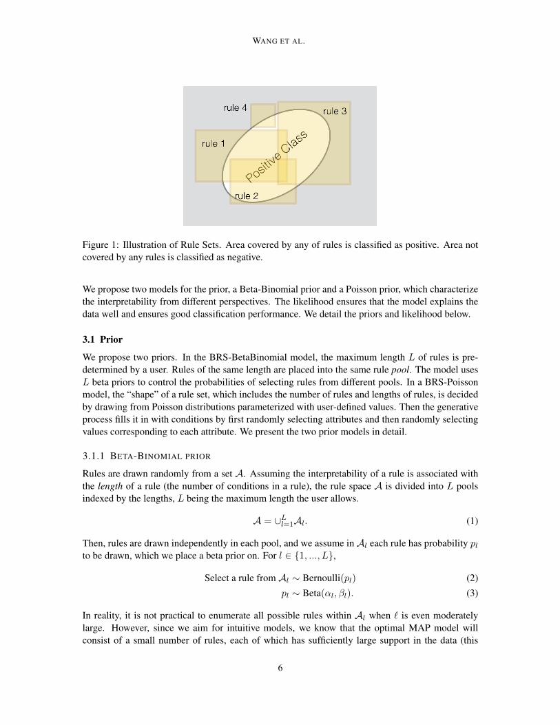
x is classified as positive if it satisfies at least one rule in A.Figure 1 shows an example of a rule set. Each rule is a yellow patch that covers a particular
area, and the rule applies to the area it covers. In Figure 1, the white oval in the middle indicates thepositive class. Our goal is to find a set of rules A that covers mostly the positive class, but little ofthe negative class, while keeping A as a small set of short rules.
We present a probabilistic model for selecting rules. Taking a generative approach allows us toflexibly incorporate users’ expectations on the “shape" of a rule set through the prior. The user canguide the model toward more domain-interpretable solutions by specifying the desired balance be-tween the size and lengths of rules without committing to any particular value for these parameters.
5
WANG ET AL.
Figure 1: Illustration of Rule Sets. Area covered by any of rules is classified as positive. Area notcovered by any rules is classified as negative.
We propose two models for the prior, a Beta-Binomial prior and a Poisson prior, which characterizethe interpretability from different perspectives. The likelihood ensures that the model explains thedata well and ensures good classification performance. We detail the priors and likelihood below.
3.1 Prior
We propose two priors. In the BRS-BetaBinomial model, the maximum length L of rules is pre-determined by a user. Rules of the same length are placed into the same rule pool. The model usesL beta priors to control the probabilities of selecting rules from different pools. In a BRS-Poissonmodel, the “shape” of a rule set, which includes the number of rules and lengths of rules, is decidedby drawing from Poisson distributions parameterized with user-defined values. Then the generativeprocess fills it in with conditions by first randomly selecting attributes and then randomly selectingvalues corresponding to each attribute. We present the two prior models in detail.
3.1.1 BETA-BINOMIAL PRIOR
Rules are drawn randomly from a set A. Assuming the interpretability of a rule is associated withthe length of a rule (the number of conditions in a rule), the rule space A is divided into L poolsindexed by the lengths, L being the maximum length the user allows.
A = ∪Ll=1Al. (1)
Then, rules are drawn independently in each pool, and we assume inAl each rule has probability plto be drawn, which we place a beta prior on. For l ∈ {1, ..., L},
Select a rule from Al ∼ Bernoulli(pl) (2)
pl ∼ Beta(αl, βl). (3)
In reality, it is not practical to enumerate all possible rules within Al when ` is even moderatelylarge. However, since we aim for intuitive models, we know that the optimal MAP model willconsist of a small number of rules, each of which has sufficiently large support in the data (this
6

BAYESIAN RULE SETS
is formalized later within proofs). Our approximate inference technique thus finds and uses highsupport rules to use within Al. This effectively makes the beta-binomial model non-parametric.
Let Ml notate the number of rules drawn from Al, l ∈ {1, ..., L}. A BRS model A consists ofrules selected from each pool. Then
p(A; {αl, βl}l) =
L∏l=1
∫pMll (1− pl)(|Al|−Ml)dpl
=L∏l=1
B(Ml + αl, |Al| −Ml + βl)
B(αl, βl), (4)
whereB(·) represents a Beta function. Parameters {αl, βl}l govern the prior probability of selectinga rule set. To favor smaller models, we would choose αl, βl such that αl
αl+βlis close to 0. In our
experiments, we set αl = 1 for all l.
3.1.2 POISSON PRIOR
We introduce a data independent prior for the BRS model. Let M denote the total number of rulesin A and Lm denote the lengths of rules for m ∈ {1, ...M}. For each rule, the length needs to be atleast 1 and at most the number of all attributes J . According to the model, we first draw M froma Poisson distribution. We then draw Lm from truncated Poisson distributions (which only allownumbers from 1 to J), to decide the “shape” of a rule set. Then, since we know the rule sizes, we cannow fill in the rules with conditions. To generate a condition, we first randomly select the attributesthen randomly select values corresponding to each attribute. Let vm,k represent the attribute indexfor the k-th condition in the m-th rule, vm,k ∈ {1, ...J}. Kvm,k is the total number of values forattribute vm,k. Note that a “value” here refers to a category for a categorical attribute, or an intervalfor a discretized continuous variable. To summarize, a rule set is constructed as follows:
1: Draw the number of rules: M ∼ Poisson(λ)2: for m ∈ {1, ...M} do3: Draw the number of conditions in m-th rule: Lm ∼ Truncated-Poisson(η), Lm ∈ {1, ...J}4: Randomly select Lm attributes from J attributes without replacement5: for k ∈ {1, ...Lm} do6: Uniformly at random select a value from Kvm,k values corresponding to attribute vm,k7: end for8: end for
We define the normalization constant ω(λ, η), so the probability of generating a rule set A is
p(A;λ, η) =1
ω(λ, η)Poisson(M ;λ)
M∏m=1
Poisson(Lm; η)1(JLm
) Lm∏k=1
1
Kvm,k
. (5)
3.2 Likelihood
LetA(xn) denote the classification outcome for xn, and let yn denote the observed outcome. Recallthat A(xn) = 1 if xn obeys any of the rules a ∈ A. We introduce likelihood parameter ρ+ to rep-resent the prior probability that yn = 1 when A(xn) = 1, and ρ− to represent the prior probability
7

WANG ET AL.
that yn = 0 when A(xn) = 0. Thus:
yn|xn, A ∼
{Bernoulli(ρ+) A(xn) = 1
Bernoulli(1− ρ−) A(xn) = 0,
with ρ+ and ρ− drawn from beta priors:
ρ+ ∼ Beta(α+, β+) and ρ− ∼ Beta(α−, β−). (6)
Based on the classification outcomes, the training data are divided into four cases: true pos-itives (TP =
∑nA(xn)yn), false positives (FP =
∑nA(xn)(1 − yn)), true negatives (TN =∑
n (1−A(xn)) (1−yn)) and false negatives (FN =∑
n (1−A(xn)) yn). Then, it can be derivedthat
p(S|A;α+, β+, α−, β−) =
∫ρTP
+ (1− ρ+)FPρTN− (1− ρ−)FNdρ+dρ−
=B(TP + α+,FP + β+)
B(α+, β+)
B(TN + α−,FN + β−)
B(α−, β−). (7)
According to (6), α+, β+, α−, β− govern the probability that a prediction is correct on trainingdata, which determines the likelihood. To ensure the model achieves the maximum likelihood whenall data points are classified correctly, we need ρ+ ≥ 1 − ρ+ and ρ− ≥ 1 − ρ−. So we chooseα+, β+, α−, β− such that α+
α++β+> 0.5 and α−
α−+β−> 0.5. Parameter tuning for the prior parame-
ters will be shown in experiments section. Let H denote a set of parameters for a data S,
H ={α+, β+, α−, β−, θprior
},
where θprior depends on the prior model, our goal is to find an optimal rule set A∗ that
A∗ ∈ arg maxA
p(A|S;H). (8)
Solving for a MAP model is equivalent to maximizing
F (A,S;H) = log p(A;H) + log p(S|A;H), (9)
where either of the two priors provided above can be used for the first term, and the likelihood is in(7). We write the objective as F (A), the prior probability of selecting A as p(A), and the likelihoodas p(S|A), omitting dependence on parameters when appropriate.
4. Approximate MAP Inference
In this section, we describe a procedure for approximately solving for the maximum a posteriori(MAP) solution to a BRS model.
Inference in Rule Set modeling is challenging because it involves a search over exponentiallymany possible sets of rules: since each rule is a conjunction of conditions, the number of rulesincreases exponentially with the number of conditions, and the number of sets of rules increasesexponentially with the number of rules. This is the reason learning a rule set has always been adifficult problem in theory.
8

BAYESIAN RULE SETS
Inference becomes easier, however, for our BRS model, due to the computational benefitsbrought by the Bayesian prior, which can effectively reduce the original problem to a much moremanageable size and significantly improve computational efficiency. Below, we detail how to ex-ploit the Bayesian prior to derive useful bounds during any search process. Here we use a stochasticcoordinate descent search technique, but the bounds hold regardless of what search technique isused.
4.1 Search Procedure
Given an objective function F (A) over discrete search space of different sets of rules and a tem-
perature schedule function over time steps, T [t] = T1− t
Niter0 , a simulated annealing (Hwang, 1988)
procedure is a discrete time, discrete state Markov Chain where at step t, given the current stateA[t],the next state A[t+1] is chosen by first randomly selecting a proposal from the neighbors, and theproposal is accepted with probability min
{1, exp
(F (A[t+1])−F (A[t])
T [t]
)}, in order to find an optimal
rule set A∗. Our version of simulated annealing is similar also to the ε-greedy algorithm used inmulti-armed bandits (Sutton and Barto, 1998).
Similar to the Gibbs sampling steps used by Letham et al. (2015); Wang and Rudin (2015) forrule-list models, here a “neighboring” solution is a rule set whose edit distance is 1 to the currentrule set (one of the rules is different). Our simulated annealing algorithm proposes a new solutionvia two steps: choosing an action from ADD, CUT and REPLACE, and then choosing a rule toperform the action on.
In the first step, the selection of which rules to ADD, CUT or REPLACE is not chosen uni-formly. Instead, the simulated annealing proposes a neighboring solution that aims to do better thanthe current model with respect to a randomly chosen misclassified point. At iteration t + 1, anexample k is drawn from data points misclassified by the current model A[t]. LetR1(xk) representa set of rules that xk satisfies, and let R0(xk) represent a set of rules that xk does not satisfy. Ifexample k is positive, it means the current rule set fails to cover it so we propose a new model thatcovers example k, by either adding a new rule from R1(xk) to A[t], or replacing a rule from A[t]
with a rule fromR1(xk). The two actions are chosen with equal probabilities. Similarly, if examplek is negative, it means the current rule set covers wrong data, and we then find a neighboring ruleset that covers less, by removing or replacing a rule from A[t] ∩R0(xk), each with probability 0.5.
In the second step, a rule is chosen to perform the action on. To choose the best rule, we evaluatethe precision of tentative models obtained by performing the selected action on each candidate rule.This precision is:
Q(A) =
∑iA(xi)yi∑iA(xi)
.
Then a choice is made between exploration, which means choosing a random rule (from the onesthat improve on the new point), and exploitation, which means choosing the best rule (the onewith the highest precision). We denote the probability of exploration as p in our search algorithm.This randomness helps to avoid local minima and helps the Markov Chain to converge to a globalminimum. We detail the three actions below.
• ADD
1. Select a rule z according to xk
9

WANG ET AL.
– With probability p, draw z randomly fromR1(xk). (Explore)– With probability 1− p, z = arg max
a∈R1(xk)Q(A[t] ∪ a). (Exploit)
2. Then A[t+1] ← A[t] ∪ z.
• CUT
1. Select a rule z according to xk
– With probability p, draw z randomly from A[t] ∩R0(xk). (Explore)– With probability 1− p, z = arg max
a∈A[t]∩R0(xk)
Q(A[t]\a). (Exploit)
2. Then A[t+1] ← A[t]\z.
• REPLACE: first CUT, then ADD.
To summarize: the proposal strategy uses an ε-greedy strategy to determine when to explore andwhen to exploit, and when it exploits, the algorithm uses a randomized coordinate descent approachby choosing a rule to maximize improvement.
4.2 Iteratively reducing rule space
Another approach to reducing computation is to directly reduce the set of rules. This dramaticallyreduces the search space, which is the power set of the set of rules. We take advantage of theBayesian prior and derive a deterministic bound on MAP BRS models that exclude rules that fail tosatisfy the bound.
Since the Bayesian prior is constructed to penalize large models, a BRS model tends to containa small number of rules. As a small number of rules must cover the positive class, each rule in theMAP model must cover enough observations. We define the number of observations that satisfy arule as the support of the rule:
supp(a) =N∑n=1
1(a(xn) = 1). (10)
Removing a rule will yield a simpler model (and a smaller prior) but may lower the likelihood.However, we can prove that the loss in likelihood is bounded as a function of the support. For a ruleset A and a rule z ∈ A, we use A\z to represent a set that contains all rules from A except z, i.e.,
A\z = {a|a ∈ A, a 6= z}.
Define
Υ =β−(N+ + α+ + β+ − 1)
(N− + α− + β−)(N+ + α+ − 1).
Then the following holds:
Lemma 1 p(S|A) ≥ (Υ)supp(z)p(S|A\z).
10

BAYESIAN RULE SETS
All proofs in this paper are in Appendix A. This lemma shows that if Υ ≤ 1, removing a rule withhigh support lowers the likelihood.
We wish to derive lower bounds on the support of rules in a MAP model. This will allowus to remove (low-support) rules from the search space without any loss in posterior. This willsimultaneously yield an upper bound on the maximum number of rules in a MAP model. Thebounds will be updated as the search proceeds.
Recall that A[τ ] denotes the rule set at time τ , and let v[t] denote the best solution found untiliteration t, i.e.,
v[t] = maxτ≤t
F (A[τ ]).
We first look at BRS-BetaBinomial models. In a BRS-BetaBinomial model, rules are selectedbased on their lengths, so there are separate bounds for rules of different lengths, and we notatethe upper bounds of the number of rules at step t as {m[t]
l }l=1,...,L, where m[t]l represents the upper
bound for the number of rules of length l.We then introduce some notations that will be used in the theorems. LetL∗ denote the maximum
likelihood of data S, which is achieved when all data are classified correctly (this holds when α+ >β+ and α− > β−), i.e. TP = N+, FP = 0, TN = N−, and FN = 0, giving:
L∗ := maxA
p(S|A) =B(N+ + α+, β+)
B(α+, β+)
B(N− + α−, β−)
B(α−, β−). (11)
For a BRS-BetaBinomial model, the following is true.
Theorem 1 Take a BRS-BetaBinomial model with parameters
H = {L,α+, β+, α−, β−, {Al, αl, βl}l=1,..L} ,
where L,α+, β+, α−, β−, {αl, βl}l=1,...L ∈ N+, α+ > β+, α− > β− and αl < βl. Define A∗ ∈arg maxA F (A) and M∗ = |A∗|. If Υ ≤ 1, we have: ∀a ∈ A∗, supp(a) ≥ C [t] and
C [t] =
log max
l
(|Al|−m
[t−1]l +βl
m[t−1]l −1+αl
)log Υ
, (12)
where
m[t]l =
logL∗ + log p(∅)− v[t]
log |Al|+βl−1
αl+m[t−1]l −1
,and m[0]
l =⌊
logL∗−log p(S|∅)log|Al|+βl−1
αl+|Al|−1
⌋and v[0] = F (∅). The size of A∗ is upper bounded by
M∗ ≤L∑l=1
m[t]l .
11

WANG ET AL.
In the equation for m[t]l , p(∅) is the prior of an empty set, which is also the maximum prior for a
rule set model, which occurs when we set αl = 1 for all l. Since L∗ and p(∅) upper bound thelikelihood and prior, respectively, logL∗ + log p(∅) upper bounds the optimal objective value. Thedifference between this value and v[t], the numerator, represents the room for improvement fromthe current solution v[t]. The smaller the difference, the smaller the m[t]
l , and thus the larger theminimum support bound. In the extreme case, when an empty set is the optimal solution, i.e., thelikelihood and the prior achieve the upper bound L∗ and p(∅) at the same time, and the optimalsolution is discovered at time t, then the numerator becomes zero and m[t]
l = 0 which preciselyrefers to an empty set. Additionally, parameters αl and βl jointly govern the probability of selectingrules of length l, according to formula (3). When αl is set to be small and βl is set to be large, plis small since E(pl) = αl
αl+βl. Therefore the resulting m[t]
l is small, guaranteeing that the algorithmwill choose a smaller number of rules overall.
Specifically, at step 0 when there is no m[t−1]l , we set m[t−1]
l = |Al|, yielding
m[0]l =
logL∗ − log p(S|∅)log |Al|+βl−1
αl+|Al|−1
, (13)
which is the upper bound we obtain before we start learning for A∗. This bound uses an empty setas a comparison model, which is a reasonable benchmark since the Bayesian prior favors smallermodels. (It is possible, for instance, that the empty model is actually close to optimal, dependingon the prior.) As log p(S|∅) increases, m[0]
l becomes smaller, which means the model’s maximumpossible size is smaller. Intuitively, if an empty set already achieves high likelihood, adding ruleswill often hurt the prior term and achieve little gain on the likelihood.
Using this upper bound, we get a minimum support which can be used to reduce the searchspace before simulated annealing begins. As m[t] decreases, the minimum support increases sincethe rules need to jointly cover positive examples. Also, if fewer rules are needed it means each ruleneeds to cover more examples.
Similarly, for BRS-Poisson models, we have:
Theorem 2 Take a BRS-Poisson model with parameters
H = {L,α+, β+, α−, β−, λ, η} ,
where L,α+, β+, α−, β− ∈ N+, α+ > β+, α− > β−. Define A∗ ∈ arg maxA F (A) and M∗ =|A∗|. If Υ ≤ 1, we have: ∀a ∈ A∗, supp(a) ≥ C [t] and
C [t] =
⌈log x
M [t]
log Υ
⌉, (14)
where
x =e−ηλmax
{(η2
)Γ(J + 1),
(η2
)J}Γ(J + 1)
,
and
M [t] =
log (λ+1)λ
Γ(λ+1)
log λ+1x
+logL∗ + log p(∅)− v[t]
log λ+1x
.12

BAYESIAN RULE SETS
The size of A∗ is upper bounded byM∗ ≤M [t].
Similar to Theorem 1, logL∗ + log p(∅) upper bounds the optimal objective value and logL∗ +log p(∅) − v[t] is an upper bound on the room for improvement from the current solution v[t]. Thesmaller the bounds becomes, the larger is the minimum support, thus reducing the rule space itera-tively whenever a new maximum solution is discovered.
The algorithm, which applies the bounds above, is given as Algorithm 1.
Algorithm 1 Inference algorithm.
procedure SIMULATED ANNEALING(Niter)A ← FP-Growth(S)A[0] ← a randomly generated rule setAmax ← A[0]
for t = 0→ Niter doA ← {a ∈ A, supp(a) ≥ C [t]} (C [t] is from (12) or (14), depending on the model choice)Sε ← misclassified examples by A[t] (Find misclassified examples)(xk, yk)← a random example drawn from Sεif yk = 1 then
action←
{ADD, with probability 0.5
REPLACE, with probability 0.5else
action←
{CUT, with probability 0.5
REPLACE, with probability 0.5
A[t+1] ← action(A, A[t],xk)Amax ← arg max(F (Amax), F (A[t+1])) (Check for improved optimal solution)α = min
{1, exp
(F (A[t+1])−F (A[t])
T [t]
)}(Probability of an annealing move)
A[t+1] ←
{A[t+1], with probability αA[t], with probability 1− α
end forreturn Amax
end procedure
4.3 Rule Mining
We mine a set of candidate rules A before running the search algorithm and only search within Ato create an approximate but more computationally efficient inference algorithm. For categorical at-tributes, we consider both positive associations (e.g., xj=‘blue’) and negative associations (xj=‘notgreen’) as conditions. (The importance of negative conditions is stressed, for instance, by Brinet al., 1997; Wu et al., 2002; Teng et al., 2002). For numerical attributes, we create a set of binaryvariables for each numerical attribute, by comparing it with a set of thresholds (usually quantiles),and add their negations as separate attributes. For example, we discretize age with three thresholds,creating six binary variables in total, i.e., age≥25, age≥50, age≥ 75 and the negations for each of
13

WANG ET AL.
them, i.e., age<25, age<50 and age<75. We then mine for frequent rules within the set of positiveobservations S+. To do this, we use the FP-growth algorithm (Borgelt, 2005), which can in practicebe replaced with any desired frequent rule-mining method.
Sometimes for large data sets with many features, even when we restrict the length of rules andthe minimum support, the number of generated rules could still be too large to handle, as it canbe exponential in the number of attributes. For example, for one of the advertisement data sets,a million rules are generated when the minimum support is 5% and the maximum length is 3. Inthat case, we use a second criterion to screen for the most potentially useful M0 rules, where M0 isuser-defined and depends on the user’s computational capacity. We first filter out rules on the lowerright plane of ROC space, i.e., their false positive rate is greater than true positive rate. Then we useinformation gain to screen rules, similarly to other works (Chen et al., 2006; Cheng et al., 2007).For a rule a, the information gain is
InfoGain(S|a) = H(S)−H(S|a), (15)
where H(S) is the entropy of the data and H(S|a) is the conditional entropy of data that split onrule a. Given a data set S, entropy H(S) is constant; therefore our screening technique chooses theM0 rules that have the smallest H(S|a).
Figure 2: All rules and selected rules on a ROC plane
We illustrate the effect of screening on one of our mobile advertisement data sets. We minedall rules with minimum support 5% and maximum length 3. For each rule, we computed its truepositive rate and false positive rate on the training data and plotted it as a dot in Figure 2. The top5000 rules with highest information gains are colored in red, and the rest are in blue. As shown inthe figure, information gain indeed selected good rules as they are closer to the upper left cornerin ROC space. For many applications, this screening technique is not needed, and we can simplyuse the entire set of pre-mined rules that have support above the required threshold for the optimalsolution provided in the theorems above.
14

BAYESIAN RULE SETS
5. Simulation Studies
We present simulation studies to show the interpretability and accuracy of our model and the effi-ciency of the simulated annealing procedure. We first demonstrate the efficiency of the simulatedannealing algorithm by searching within candidate rules for a “true rule set" that generates the data.Simulations show that our algorithm can recover the true rule set with high probability within asmall number of iterations despite the large search space. We then designed the second set of sim-ulations to study the trade-off between accuracy and simplicity. BRS models may lose accuracyto gain model simplicity when the number of attributes is large. Combining the two simulationsstudies, we were able to hypothesize that possible losses in accuracy are often due to the choiceof model representation as a rule set, rather than simulated annealing. In this section, we choosethe BRS-BetaBinomial model for the experiments. BRS-Poisson results would be similar; the onlydifference is the choice of prior.
5.1 Simulation Study 1: Efficiency of Simulated Annealing
In the first simulation study, we would like to test if simulated annealing is able to recover a truerule set given that these rules are in a candidate rule set, and we would like to know how efficientlysimulated annealing finds them. Thus we omit the step of rule mining for this experiment anddirectly work with generated candidate rules, which we know in this case contains a true rule set.
Let there be N observations, {xn}n=1,...,N and a collection of M candidate rules, {am}m=1,...M .We can construct an N ×M binary matrix where the entry in the n-th row and m-th column is theBoolean function am(xn) that represents whether the n-th observation satisfies the m-th rule. Letthe true rule set be a subset of the candidate rules, A∗ ⊂ {am}m=1,...M . The labels {yn}n=1,...N
satisfy
yn =
{1 ∃a ∈ A∗, a(xn) = 1
0 otherwise.(16)
We ran experiments with varying N and M . Each time, we first generated an N ×M binarymatrix by setting the entries to 1 with probability 0.035, and then selected 20 columns to form A∗.(Values 0.035 and 20 are chosen so that the positive class contains roughly 50% of the observations.We also ensured that the 20 rules do not include each other.) Then {yn}n=1,...N were generated asabove. We randomly assigned lengths from 1 to 5 to {am}m=1,...M . Finally, we ran Algorithm 1 onthe data set. The prior parameters were set as below for all simulations:
αl = 1, βl = |Al| for l = 1, ..., 3,
α+ = α− = 1000, β+ = β− = 1.
For each pair of N and M , we repeated the experiment 100 times and recorded intermediateoutput models at different iterations. Since multiple different rule sets can cover the same points,we compared labels generated from the true rule set and the recovered rule set: a label is 1 if theinstance satisfies the rule set and 0 otherwise. We recorded the training error for each intermediateoutput model. The mean and standard deviation of training error rate are plot Figure 3, along withrun time to convergence in seconds on the right figure.
Comparing the three sets of experiments, we notice that different sizes of the binary matrix ledto differing convergence times due to different computation cost of handling the matrices, yet thethree error rate curves in Figure 3 almost completely overlap. Neither the size of the data set N nor
15

WANG ET AL.
Figure 3: Convergence of mean error rate with number of iterations for data with varying N and Mand running time (in seconds), obtained by the BRS-BetaBinomial.
the size of the rule space M affected the search. This is because the strategy based on curiosity andbounds chose the best solution efficiently, regardless of the size of data or the rule space.
More importantly, this study shows that simulated annealing is able to recover a true rule setA∗, or an equivalent rule set with optimal performance, with high probability, with few iterations.
5.2 Simulation Study 2: Accuracy-Interpretability Trade-off
We observe from the first simulation study that simulated annealing does not tend to cause losses inaccuracy. In the second simulation study, we would like to identify whether the rule representationcauses losses in accuracy. In this study, we used the rule mining step and directly worked with data{xn}n=1,...,N . Without loss of generality, we assume xn ∈ {0, 1}J .
In each experiment, we first constructed an N × J binary matrix {xn}n=1,...N by setting theentries to 1 with probability 0.5, then randomly generated 20 rules from {xn}n=1,...,N to form A∗
and finally generated labels {yn}n=1,...,N following formula (16). We checked the balance of thedata before pursuing the experiment. The data set was used only if the positive class was within[30%, 70%] of the total data, and otherwise regenerated.
To constrain computational complexity, we set the maximum length of rules to be 7 and thenselected the top 5000 rules with highest information gain. Then we performed Algorithm 1 on thesecandidate rules to generate a BRS model A. Ideally, A should be simpler than A∗, with a possibleloss in its accuracy as a trade-off.
To study the influence of the dimensions of data on accuracy and simplicity, we varied N andJ and repeated each experiment 100 times. Figure 4 shows the accuracy and number of rules in Ain each experiment. The number of rules in A was almost always less than the number of rules inA∗ (which was 20). On average, A contained 12 rules, which was 60% of the size of A∗, slightlycompromising accuracy. BRS needed to compromise more when J was large since it became harderto maintain the same level of simplicity.
16

BAYESIAN RULE SETS
Figure 4: Accuracy and complexity of output BRS models for data with varying N and J , obtainedfrom the BRS-BetaBinomial.
We show in Figure 5 the average training error at different iterations to illustrate the convergencerate. Simulated annealing took less than 50 iterations to converge. Note that it took fewer iterationsthan simulation study 1 since the error rate curve started from less than 0.5, due to rule pre-screeningusing information gain.
Figure 5: Convergence of mean error rate with varying N and J , obtained by BRS-BetaBinomial.
Figure 4 and Figure 5 both indicate that increasing the number of observations did not affectthe performance of the model. BRS is more sensitive to the number of attributes. The larger J is,the less informative a short rule becomes to describe and distinguish a class in the data set, and themore BRS has to trade-off, in order to keep simple rules within the model.
To summarize: when we model using fewer rules, it benefits interpretability but can lose infor-mation. Rules with a constraint on the maximum length tend to be less accurate when dealing with
17

WANG ET AL.
high dimensional feature spaces. The loss increases with the number of features. This is the pricepaid for using an interpretable model. There is little price paid for using our optimization method.
6. Experiments
Our main application of interest is mobile advertising. We collected a large advertisement data setusing Amazon Mechanical Turk that we made publicly available (Wang et al., 2015), and we testedBRS on other publicly available data sets. We show that our model can generate interpretable resultsthat are easy for humans to understand, without losing too much (if any) predictive accuracy. Insituations where the ground truth consists of deterministic rules (similarly to the simulation study),our method tends to perform better than other popular machine learning techniques.
6.1 UCI Data Sets
We test BRS on ten data sets from the UCI machine learning repository (Bache and Lichman, 2013)with different types of attributes; four of them contain categorical attributes, three of them containnumerical attributes and three of them contain both. We performed 5-fold cross validation on eachdata set. Since our goal was to produce models that are accurate and interpretable, we set themaximum length of rules to be 3 for all experiments. We compared with interpretable algorithms:Lasso (without interaction terms to preserve interpretability), decision trees (C4.5 and CART), andinductive rule learner RIPPER (Cohen, 1995), which produces a rule list greedily and anneals locallyafterward. In addition to interpretable models, we also compare BRS with uninterpretable modelsfrom random forests and SVM to set a benchmark for expected accuracy on each data set. We usedimplementations of baseline methods from R packages, and tuned model parameters via 5-foldnested cross validation.
Table 1: Accuracy of each comparing algorithm (mean ± std) on ten UCI data sets.
DataBRS1 BRS2 Lasso C4.5 CART RIPPER
RandomSVM
Type Forest
connect-4
Categorical
.76±.01 .75±.01 .70±.00 .83±.00 .69±.01 ———- .86±.00 .82±.00mushroom 1.00±.00 1.00±.00 .96±.00 1.00±.00 .99±.00 .99±.00 1.00±.00 .93±.00tic-tac-toe 1.00±.00 1.00±.00 .71±.02 .92±.03 .93±.02 .98±.01 .99±.00 .99±.00chess .89±.01 .89±.01 .83±.01 .97±.00 .92±.04 .91±.01 .91±.00 .99±.00magic
Numerical.80±.02 .79±.01 .76±.01 .79±.00 .77±.00 .78±.00 .78±.01 .78±.01
banknote .97±.01 .97±.01 1.00±.00 .90±.01 .90±.02 .91±.01 .91±.01 1.00±.00indian-diabetes .72±.03 .73±.03 .67±.01 .66±.03 .67±.01 .67±.02 .75±.03 .69±.01adult
Mixed.83±.00 .84±.01 .82±.02 .83±.00 .82±.01 .83±.00 .84±.00 .84±.00
bank-marketing .91±.00 .91±.00 .90±.00 .90±.00 .90±.00 .90±.00 .90±.00 .90±.00heart .85±.03 .84±.03 .85±.04 .76±.06 .77±.06 .78±.04 .81±.06 .86±.06
Rank of accuracy 2.6±1.7 2.6±1.8 5.4±2.8 4.3±2. 9 5.6±1.8 4.8±1.5 2.7±1.7 2.8±2.2
Table 1 displays the means and standard deviations of the test accuracy for all algorithms(the lead author’s laptop ran out of memory when applying RIPPER to the connect-4 data set),
18

BAYESIAN RULE SETS
Table 2: Runtime (in seconds) of each comparing algorithm (mean ± std) on ten UCI data sets.
BRS1 BRS2 Lasso C4.5 CART RIPPERRandom
SVMForest
connect-4 288.1±22.2 279.1±20.9 0.9±0.0 30.4±0.6 20.5±0.4 ———- 746.6±14.9 1427.8±35.1mushroom 8.8±1.3 8.18±1.3 0.1±0.0 0.5±0.0 0.6±0.0 1.2±0.1 15.6±0.8 23.5±1.2tic-tac-toe 1.0±0.0 1.0±0.0 0.0±0.0 0.1±0.0 0.1±0.0 0.3±0.0 1.3±.0.0 0.2±0.0chess 44.8±8.2 41.6±8.2 0.1±0.0 1.3±0.4 0.3±0.1 50.6±18.0 47.5±1.9 1193.3±79.6magic 31.3±4.4 29.3±4.4 0.1±0.0 1.4±0.1 2.3±0.2 8.8±1.7 43.5±1.3 139.7±3.2banknote 1.0±0.1 0.9±0.1 0.0±0.0 0.1±0.0 0.1±0.0 0.2±0.0 1.1±0.0 0.1±0.0indian-diabetes 0.6±0.1 0.6±0.1 0.0±0.0 0.1±0.0 0.1±0.0 0.2±0.0 0.7±0.0 0.2±0.0adult 50.2±6.2 47.1±6.2 0.4±0.0 9.8±0.3 10.7±0.4 66.0±8.8 344.4±7.7 174.6±4.7bank-marketing 55.2±2.7 50.8±2.7 0.4±0.0 11.6±0.6 7.6±0.3 23.9±4.6 320.0±9.8 395.1±28.1heart 0.5±0.1 0.5±0.1 0.0±0.0 0.1±0.0 0.0±0.0 0.2±0.1 0.3±0.0 0.0±0.0
and the rank of their average performance. Table 2 displays the runtime. BRS1 represents BRS-BetaBinomial and BRS2 represents BRS-Poisson. While BRS models were under strict restrictionfor interpretability purposes (L = 3), BRS’s performance surpassed that of the other interpretablemethods and was on par with uninterpretable models. This is because, firstly, BRS has Bayesianpriors that favor rules with a large support (Theorem 1, 2) which naturally avoids overfitting ofthe data; and secondly, BRS optimizes a global objective while decision trees and RIPPER rely onlocal greedy splitting and pruning methods, and interpretable versions of Lasso are linear in thebase features. Decision trees and RIPPER are local optimization methods and tend not to have thesame level of performance as globally optimal algorithms, such as SVM, Random Forests, BRS,etc. The class of rule set models and decision tree models are the same: both create regions withininput space consisting of a conjunction of conditions. The difference is the choice of optimizationmethod: global vs. local.
For the tic-tac-toe data set, the positive class can be classified using exactly eight rules. BRS hasthe capability to exactly learn these conditions, whereas the greedy splitting and pruning methodsthat are pervasive throughout the data mining literature (e.g., CART, C4.5) and convexified approx-imate methods (e.g., SVM) have difficulty with this. Both linear models and tree models exist thatachieve perfect accuracy, but the heuristic splitting/pruning and convexification of the methods wecompared with prevented these perfect solutions from being found.
BRS achieves accuracies competitive to uninterpretable models while requiring a much shorterruntime, which grows slowly with the size of the data, unlike Random forest and SVM. This indi-cates that BRS can reliably produce a good model within a reasonable time for large data sets.
6.1.1 PARAMETER TUNING
A MAP solution maximizes the sum of logs of prior and likelihood. The scale of the prior andlikelihood directly determines how the model trades off between fitting the data and achievingthe desired sparsity level. Again, we choose the BRS-BetaBinomial for this demonstration. TheBayesian model uses parameters {αl, βl}Ll=1 to govern the prior for selecting rules and parametersα+, β+, α−, β− to govern the likelihood of data. We study how sensitive the results are to different
19

WANG ET AL.
parameters and how to tune the parameters to get the best performing model. We choose one dataset from each category from Table 1.
We fixed the prior parameters αl = 1, βl = |Al| for l = 1, .., L, and only varied likelihoodparameters α+, β+, α−, β− to analyze how the performance changes as the magnitude and ratioof the parameters change. To simplify the study, we took α+ = α− = α, and β+ = β− = β.We let s = α + β and s was chosen from {100, 1000, 10000}. We let ρ = α
α+β and ρ variedwithin [0, 1]. Here, s and ρ uniquely define α and β. We constructed models for different s and ρand plotted the average out-of-sample accuracy as s and ρ changed in Figure 6 for three data setsrepresentative of categorical, numerical and mixed data types. The X axis represents ρ and Y axisrepresents s. Accuracies increase as ρ increases, which is consistent with the intuition of ρ+ andρ−. The highest accuracy is always achieved at the right half of the curve. The performance is lesssensitive to the magnitude s and ratio ρ, especially when ρ > 0.5. For tic-tac-toe and diabetes, theaccuracy became flat once ρ becomes greater than a certain threshold, and the performance was notsensitive to ρ either after that point; it is important as it makes tuning the algorithm easy in practice.Generally, taking ρ close to 1 leads to a satisfactory output. Table 1 and 2 were generated by modelswith ρ = 0.9 and s = 1000.
Figure 6: Parameter tuning experiments. Accuracy vs. ρ for all data sets. X axis represents ρ and Yaxis represents accuracy.
6.1.2 DEMONSTRATION WITH TIC-TAC-TOE DATA
Let us illustrate the reduction in computation that comes from the bounds in the theorems in Section4. For this demonstration, we chose the tic-tac-toe data set since the data can be classified exactlyby eight rules which are naturally an underlying true rule set, and our method recovered the rulessuccessfully, as shown in Table 1. We use BRS-BetaBinomial for this demonstration.
First, we used FP-Growth (Borgelt, 2005) to generate rules. At this step, we find all possiblerules with length between 1 to 9 (the data has 9 attributes) and has minimum support of 1 (the rule’sitemset must appear at least once int the data set). FP-growth generates a total of 84429 rules. Wethen set the hyper-parameters as:
αl = 1, βl = |Al| for l = 1, ..., 9,
α+ = N+ + 1, β+ = N+, α− = N− + 1, β− = N−.
We ran Algorithm 1 on this data set. We kept a list of the best solutions v[t] found until time tand updated m[t−1]
l and the minimum support with the new v[t] according to Theorem 1. We showin Figure 7 the minimum support at different iterations whenever a better v[t] is obtained. Within
20

BAYESIAN RULE SETS
Figure 7: Updated minimum support at different iterations
ten iterations, the minimum support increased from 1 to 9. If, however, we choose a stronger priorfor small models by increasing βl to 10 times |Al| for all l and keeping all the other parametersunchanged, then the minimum support increases even faster and reached 13 very quickly. This isconsistent with the intuition that if the prior penalizes large models more heavily, the output tendsto have a smaller size. Therefore each rule will need to cover more data.
Placing a bound on the minimum support is critical for computation since the number of possiblerules decays exponentially with the support, as shown in Figure 8a. As the minimum support isincreased, more rules are removed from the original rule space. Figure 8a shows the percentage ofrules left in the solution space as the minimum threshold is increased from 1 to 9 and to 13. At aminimum support of 9, the rule space is reduced to 9.0% of its original size; at a minimum supportof 13, the rule space is reduced to 4.7%. This provides intuition of the benefit of Theorem 1.
(a) Reduced rule space as the minimum support increases (b) Number of rules of different lengths mined at differentminimum support.
Figure 8: Demonstration with Tic-Tac-Toe data set
Although rules are filtered out based on their support, we observe that longer rules are moreheavily reduced than shorter rules. This is because the support of a rule is negatively correlated withits length, as the more conditions a rule contains, the fewer observations can satisfy it. Figure 8bshows distributions of rules across different lengths when mined at different minimum support lev-
21
WANG ET AL.
els. Before any filtering (i.e., C = 1), more than half of the rules have lengths greater than 5. As Cis increased to 9 and 13, these long rules are almost completely removed from the rule space.
To summarize, the strength of the prior is important for computation, and changes the nature ofthe problem: a stronger prior can dramatically reduce the size of the search space. Any increasein minimum support, that the prior provides, leads to a smaller search by the rule mining methodand a smaller optimization problem for the BRS algorithm. These are multiple order-of-magnitudedecreases in the size of the problem.
6.2 Application to In-vehicle Recommendation System
For this experiment, our goal was to understand customers’ response to recommendations made inan in-vehicle recommender system that provides coupons for local businesses. The coupons wouldbe targeted to the user in his/her particular context. Our data were collected on Amazon MechanicalTurk via a survey that we will describe shortly. We used Turkers with high ratings (95% or above).Out of 752 surveys, 652 were accepted, which generated 12684 data cases (after removing rowscontaining missing attributes).
The prediction problem is to predict if a customer is going to accept a coupon for a particularvenue, considering demographic and contextual attributes. Answers that the user will drive there‘right away’ or ‘later before the coupon expires’ are labeled as ‘Y = 1’ and answers ‘no, I do notwant the coupon’ are labeled as ‘Y = 0’. We are interested in investigating five types of coupons:bars, takeaway food restaurants, coffee houses, cheap restaurants (average expense below $20 perperson), expensive restaurants (average expense between $20 to $50 per person). In the first part ofthe survey, we asked users to provide their demographic information and preferences. In the secondpart, we described 20 different driving scenarios (see examples in Appendix B) to each user alongwith additional context information and coupon information (see Appendix B for a full descriptionof attributes) and asked the user if s/he will use the coupon.
For this problem, we wanted to generate simple BRS models that are easy to understand. So werestricted the lengths of rules and the number of rules to yield very sparse models. Before miningrules, we converted each row of data into an item which is an attribute and value pair. For categoricalattributes, each attribute-value pair was directly coded into a condition. Using marital status as anexample, ‘marital status is single’ was converted into (MaritalStatus: Single), (MaritalStatus: NotMarried partner), and (MaritalStatus: Not Unmarried partner), (MaritalStatus: Not Widowed). Fordiscretized numerical attributes, the levels are ordered, such as: age is ‘20 to 25’, or ‘26 to 30’, etc.;additionally, each attribute-value pair was converted into two conditions, each using one side of therange. For example, age is ‘20 to 25’ was converted into (Age:>=20) and (Age:<=25). Then eachcondition is a half-space defined by threshold values. For the rule mining step, we set the minimumsupport to be 5% and set the maximum length of rules to be 4. We used information gain in Equation(15) to select the best 5000 rules to use for BRS. We ran simulated annealing for 50000 iterationsto obtain a rule set.
We compared with interpretable classification algorithms that span the space of widely usedmethods that are known for interpretability and accuracy, C4.5, CART, Lasso, RIPPER, and a naïvebaseline using top K rules, referred to as TopK. For C4.5, CART, Lasso, and RIPPER, we used theRWeka package in R and tuned the hyper-parameters to generate different models on a ROC plane.For the TopK method, we varied K from 1 to 10 to produce ten models using best K pre-minedrules ranked by the information gain in Equation (15). For BRS, We varied the hyperparameters
22

BAYESIAN RULE SETS
α+, β+, α−, β− to obtain different sets of rules. For all methods, we picked models on their ROCfrontiers and reported their performance below.
Performance in accuracy To compare their predictive performance, we measured out-of-sampleAUC (the Area Under The ROC Curve) from 5-fold testing for all methods, reported in Table 3.The BRS classifiers, while restricted to produce sparse disjunctions of conjunctions, had betterperformance than decision trees and RIPPER, which use greedy splitting and pruning methods,and do not aim to globally optimize. TopK’s performance was substantially below that of othermethods. BRS models are also comparable to Lasso, but the form of the model is different. BRSmodels do not require users to cognitively process coefficients.
BarTakeaway
FoodCoffee House
CheapRestaurant
ExpensiveRestaurant
BRS1 0.773 (0.013) 0.682 (0.005) 0.760 (0.010) 0.736 (0.022) 0.705 (0.025)BRS2 0.776 (0.011) 0.667 (0.023) 0.762 (0.007) 0.736 (0.019) 0.707 (0.030)C4.5 0.757 (0.015) 0.602 (0.051) 0.751 (0.018) 0.692 (0.033) 0.639 (0.027)CART 0.772 (0.019) 0.615 (0.035) 0.758 (0.013) 0.732 (0.018) 0.657 (0.010)Lasso 0.795 (0.014) 0.673 (0.042) 0.786 (0.011) 0.769 (0.024) 0.706 (0.017)RIPPER 0.762 (0.015) 0.623 (0.048) 0.762(0.012) 0.705(0.023) 0.689 (0.034)TopK 0.562 (0.015) 0.523 (0.024) 0.502(0.012) 0.582(0.023) 0.508 (0.011)
Table 3: AUC comparison for mobile advertisement data set, means and standard deviations overfolds are reported.
Performance in complexity For the same experiment, we would also like to know the complexityof all methods at different accuracy levels. Since the methods we compare have different structures,there is not a straightforward way to directly compare complexity. However, decision trees can beconverted into equivalent rule set models. For a decision tree, an example is classified as positive ifit falls into any positive leaf. Therefore, we can generate equivalent models in rule set form for eachdecision tree, by simply collecting branches with positive leaves. Therefore, the four algorithmswe compare, C4.5, CART, RIPPER, and BRS have the same form. To measure the complexity, wecount the total number of conditions in the model, which is the sum of lengths for all rules. Thisloosely represents the cognitive load needed to understand a model. For each method, we take themodels that are used to compute the AUC in Table 3 and plot their accuracy and complexity inFigure 9. BRS models achieved the highest accuracy at the same level of complexity. This is notsurprising given that BRS performs substantially more optimization than other methods.
To show that the benefits of BRS did not come from rule mining or screening using heuristics,we compared the BRS models with TopK models that rely solely on rule mining and ranking withheuristics. Figure 10 shows there is a substantial gain in the accuracy of BRS models compared toTopK models.
From Table 3 we observe that Lasso achieved consistently good AUC. For the five coupons, theaverage number of nonzero coefficients for lasso models in different folds are 93, 94.6, 90.2, 93.2and 93.4, which is on the order of ∼20 times larger than the number of conditions used in BRS andother rule based models; in this case, the lasso models are not interpretable.
23

WANG ET AL.
Figure 9: Test accuracy vs complexity for BRS and other models on mobile advertisement data setsfor different coupons
Figure 10: Test accuracy vs complexity for BRS and TopK on mobile advertisement data sets fordifferent coupons
Examples of BRS models In practice, for this particular application, the benefits of interpretabil-ity far outweigh small improvements in accuracy. An interpretable model can be useful to a vender
24

BAYESIAN RULE SETS
choosing whether to provide a coupon and what type of coupon to provide, it can be useful to usersof the recommender system, and it can be useful to the designers of the recommender system tounderstand the population of users and correlations with successful use of the system. As discussedin the introduction, rule set classifiers are particularly natural for representing consumer behavior,particularly consideration sets, as modeled here.
We show several classifiers produced by BRS in Figure 11, where the curves were produced bymodels from the experiments discussed above. Example rule sets are listed in each box along thecurve. For instance, the classifier near the middle of the curve in Figure 11 (a) has one rule, and reads“If a person visits a bar at least once per month, is not traveling with kids, and their occupation isnot farming/fishing/forestry, then predict the person will use the coupon for a bar before it expires."In these examples (and generally), we see that a user’s general interest in a coupon’s venue (bar,coffee shop, etc.) is the most relevant attribute to the classification outcome; it appears in every rulein the two figures.
(a) Coupons for bars (b) Coupons for coffee houses
Figure 11: ROC for data set of coupons for bars and coffee houses.
7. Conclusion
We presented a method that produces rule set (disjunctive normal form) models, where the shapeof the model can be controlled by the user through Bayesian priors. In some applications, such asthose arising in customer behavior modeling, the form of these models may be more useful thantraditional linear models. Since finding sparse models is computationally hard, most approachestake severe heuristic approximations (such as greedy splitting and pruning in the case of decisiontrees, or convexification in the case of linear models). These approximations can severely hurtperformance, as is easily shown experimentally, using data sets whose ground truth formulas are notdifficult to find. We chose a different type of approximation, where we make an up-front statisticalassumption in building our models out of pre-mined rules, and aim to find the globally optimal
25

WANG ET AL.
solution in the reduced space of rules. We then find theoretical conditions under which using pre-mined rules provably does not change the set of MAP optimal solutions. These conditions relatethe size of the data set to the strength of the prior. If the prior is sufficiently strong and the dataset is not too large, the set of pre-mined rules is provably sufficient for finding an optimal rule set.We showed the benefits of this approach on a consumer behavior modeling application of currentinterest to “connected vehicle" projects. Our results, using data from an extensive survey taken byseveral hundred individuals, show that simple rules based on a user’s context can be directly usefulin predicting the user’s response.
Appendix A.
Proof 1 (of Lemma 1) Let TP, FP, TN, and FN be the number of true positives, false positives, truenegatives and false negatives in S classified by A. We now compute the likelihood for model A\z .The most extreme case is when rule z is an 100% accurate rule that applies only to real positivedata points and those data points satisfy only z. Therefore once removing it, the number of truepositives decreases by supp(z) and the number of false negatives increases by supp(z). That is,
p(S|A\z) ≥B(TP− supp(z) + α+,FP + β+)
B(α+, β+)
B(TN + α−,FN + supp(z) + β−)
B(α−, β−)
=p(S|A) · g3(supp(z)), (17)
where
g3(supp(z)) =Γ(TP + α+ − supp(z))
Γ(TP + α+)
Γ(TP + FP + α+ + β+)
Γ(TP + FP + α+ + β+ − supp(z))(18)
Γ(FN + β− + supp(z))
Γ(FN + β−)
Γ(TN + FN + α− + β−)
Γ(TN + FN + α− + β− + supp(z)). (19)
Now we break down g3(supp(z)) to find a lower bound for it. The first two terms in (18) become
Γ(TP + α+ − supp(z))
Γ(TP + α+)
Γ(TP + FP + α+ + β+)
Γ(TP + FP + α+ + β+ − supp(z))
=(TP + FP + α+ + β+ − supp(z)) . . . (TP + FP + α+ + β+ − 1)
(TP + α+ − supp(z)) . . . (TP + α+ − 1)
≥(
TP + FP + α+ + β+ − 1
TP + α+ − 1
)supp(z)
≥(N+ + α+ + β+ − 1
N+ + α+ − 1
)supp(z)
. (20)
26

BAYESIAN RULE SETS
Equality holds in (20) when TP = N+,FP = 0. Similarly, the last two terms in (18) become
Γ(FN + β− + supp(z))
Γ(FN + β−)
Γ(TN + FN + α− + β−)
Γ(TN + FN + α− + β− + supp(z))
=(FN + β−) . . . (FN + β− + supp(z)− 1)
(TN + FN + α− + β−) . . . (TN + FN + α− + β− + supp(z)− 1)
≥(
FN + β−FN + TN + α− + β−
)supp(z)
≥(
β−N− + α− + β−
)supp(z)
. (21)
Equality in (21) holds when TN = N−,FN = 0. Combining (17), (18), (20) and (21), we obtain
P (S|A\z) ≥(N+ + α+ + β+ − 1
N+ + α+ − 1
β−N− + α− + β−
)supp(z)
· p(S|A)
= Υsupp(z)p(S|A). (22)
Proof 2 (of Theorem 1)Step 1 We first prove the upper bound m[t]
l . Since A∗ ∈ arg maxA F (A), F (A∗) ≥ v[t], i.e.,
log p(S|A∗) + log p(A∗) ≥ v[t]. (23)
We then upper bound the two terms on the left-hand-side.Let M∗l denote the number of rules of length l in A∗. The prior probability of selecting A∗ from
A is
p(A∗) = p(∅)L∏l=1
B(Ml + αl, |Al| −Ml + βl)
B(αl, |Al|+ βl).
We observe that when 0 ≤M∗l ≤ |Al|,
B(Ml + αl, |Al| −Ml + βl) ≤ B(αl, |Al|+ βl),
giving
p(A∗) ≤ p(∅)B(Ml′ + αl′ , |Al′ | −Ml′ + βl′)
B(αl′ , |Al′ |+ βl′)
= p(∅)αl′ · (αl′ + 1) · · · (M∗l′ + αl′ − 1)
(|Al′ | −M∗l′ + βl′) · · · (|Al′ |+ βl′ − 1)
≤ p(∅)(M∗l′ + αl′ − 1
|Al′ |+ βl′ − 1
)M∗l′
(24)
for all l′ ∈ {1, ..., L}. The likelihood is upper bounded by
p(S|A∗) ≤ L∗. (25)
Substituting (24) and (25) into (23) we get
logL∗ + log p(∅) +M∗l′ log
(M∗l′ + αl′ − 1
|Al′ |+ βl′ − 1
)≥ v[t], (26)
27

WANG ET AL.
which gives
M∗l′ ≤logL∗ + log p(∅)− v[t]
log(|Al′ |+βl′−1M∗l′+αl′−1
)≤ logL∗ + log p(∅)− v[t]
log
(|Al′ |+βl′−1
m[t−1]
l′ +αl′−1
) , (27)
where (27) follows because m[t−1]l′ is an upper bound on M∗l′ . Since M∗l′ has to be an integer, we get
M∗l′ ≤
logL∗ + log p(∅)− v[t]
log
(|Al′ |+βl′−1
m[t−1]
l′ +αl′−1
)
= m[t]l′ for all l′ ∈ {1, ..., L}. (28)
Thus
M∗ =L∑l=1
M∗l ≤L∑l=1
m[t]l . (29)
Step 2: Now we prove the lower bound on the support. We would like to prove that a MAP modeldoes not contain rules of support less than a threshold. To show this, we prove that if any rule z hassupport smaller than some constant C, then removing it yields a better objective, i.e.,
F (A) ≤ F (A\z). (30)
Our goal is to find conditions on C such that this inequality holds. Assume in rule set A, Ml comesfrom pool Al of rules with length l, l ∈ {1, ...L}, and rule z has length l′ so it is drawn from Al′ .
A\z consists of the same rules as A except missing one rule from Al′ . We must have:
p(A\z) =B(Ml′ + αl′ , |Al′ | −Ml′ + βl′)
B(αl′ , βl′)·∏l 6=l′
B(Ml + αl, |Al| −Ml + βl)
B(αl, βl)
=p(A) · B(Ml′ + αl′ , |Al′ | −Ml′ + βl′)
B(Ml′ + 1 + αl′ , |Al′ | −Ml′ − 1 + βl′)
=p(A) · |Al′ | −Ml′ + βl′
Ml′ − 1 + αl′.
|Al′ |−Ml′+βl′Ml′−1+αl′
decreases monotonically as Ml′ increases, so it is lower bounded at the upper bound
on Ml′ , m[t]l′ , obtained in step 1. Therefore
|Al′ | −Ml′ + βl′
Ml′ − 1 + αl′≥|Al′ | −m
[t]l′ + βl′
m[t]l′ − 1 + αl′
for l′ ∈ {1, ...L}.
28

BAYESIAN RULE SETS
Thus
p(A\z) ≥ maxl
(|Al| −m
[t]l + βl
m[t]l − 1 + αl
)p(A). (31)
Combining (31) and Lemma 1, the joint probability of S and A\z is bounded by
P (S,A\z) =p(A\z)P (S|A\z)
≥maxl
(|Al| −m
[t]l + βl
m[t]l − 1 + αl
)(Υ)supp(z) · P (S,A).
In order to get P (S,A\z) ≥ P (S,A), and with Υ ≤ 1 from the assumption in the theorem’sstatement, we must have
supp(z) ≤log max
l
(|Al|−m
[t]l +βl
m[t]l −1+αl
)log Υ
.
This means if ∃z ∈ A such that supp(z) ≤log max
l
(|Al|−m
[t]l
+βl
m[t]l−1+αl
)log Υ , then A 6∈ arg maxA′ F (A′),
which is equivalent to saying, for any z ∈ A∗,
supp(z) ≥log max
l
(|Al|−m
[t]l +βl
m[t]l −1+αl
)log Υ
.
Since the support of a rule has to be integer,
supp(z) ≥
log max
l
(|Al|−m
[t]l +βl
m[t]l −1+αl
)log Υ
.Before proving Theorem 2, we first prove the following lemma that we will need later.
Lemma 2 Define a function g(l) =(λ2
)lΓ(J − l + 1), λ, J ∈ N+. If 1 ≤ l ≤ J ,
g(l) ≤ max
{(λ
2
)Γ(J + 1),
(λ
2
)J}.
Proof 3 (Of Lemma 2) In order to bound g(l), we will show that g(l) is convex, which means itsmaximum value occurs at the endpoints of the interval we are considering. The second derivativeof g(l) respect to l is
g′′(l) = g(l)
(lnλ
2+ γ −
∞∑k=1
1
k− 1
k + J − Lm
)2
+∞∑k=1
1
(k + J − l)2
> 0, (32)
29

WANG ET AL.
since at least one of the terms 1(k+J−l)2 > 0. Thus g(l) is strictly convex. Therefore the maximum
of g(l) is achieved at the boundary of Lm, namely 1 or J . So we have
g(l) ≤ max {g(1), g(J)}
= max
{(λ
2
)Γ(J + 1),
(λ
2
)J}. (33)
Proof 4 (Of Theorem 2) We follow similar steps in the proof for Theorem 1.Step 1 We first derive an upper bound M∗ at time t, denoted as M [t].
The probability of selecting a rule set A∗ depends on the number of rules M∗ and the length ofeach rule, which we denote as Lm,m ∈ {1, ...,M∗}, so the prior probability of selecting A∗ is
P (A∗; θ) = ω(λ, η)Poisson(M∗;λ)
M∗∏m
Poisson(Lm; η)1(JLm
) Lm∏k
1
Kvm,k
= p(∅) λM∗
Γ(M∗ + 1)
M∗∏m
e−ηηLmΓ(J − Lm + 1)
Γ(J + 1)
Lm∏k
1
Kvm,k
≤ p(∅) 1
Γ(M∗ + 1)
(e−ηλ
Γ(J + 1)
)M∗ M∗∏m
(η2
)LmΓ(J − Lm + 1). (34)
(34) follows from Kvm,k ≥ 2 since all attributes have at least two values. Using Lemma 2 wehave that (η
2
)LmΓ(J − Lm + 1) ≤ max
{(η2
)Γ(J + 1),
(η2
)J}. (35)
Combining (34) and (35), and the definition of x, we have
P (A∗; θ) ≤ p(∅) xM∗
Γ(M∗ + 1). (36)
Now we apply (23) combining with (36) and (25), we get
logL∗ + log p(∅) + logxM
∗
Γ(M∗ + 1)≥ v[t] (37)
Now we want to upper bound xM∗
Γ(M∗+1) .If M∗ ≤ λ, the statement of the theorem holds trivially. For the remainder of the proof we
consider, if M∗ > λ, xM∗
Γ(M∗+1) is upper bounded by
xM∗
M∗!≤ xλ
λ!
x(M∗−λ)
(λ+ 1)(M∗−λ),
where in the denominator we used Γ(M∗+1) = Γ(λ+1)(λ+1) · · ·M∗ ≥ Γ(λ+1)(λ+1)(M∗−λ).So we have
logL∗ + log p(∅) + logxλ
Γ(λ+ 1)+ (M − λ) log
x
λ+ 1≥ v[t]. (38)
30

BAYESIAN RULE SETS
We have xλ+1 ≤ 1. To see this, note Γ(J)
Γ(J+1) < 1, e−η(η
2
)< 1 and
e−η( η2 )J
Γ(J+1) < 1 for every η and J .Then solving for M∗ in (38), using x
λ+1 < 1 to determine the direction of the inequality yields:
M∗ ≤M [t] =
λ+logL∗ + log p(∅) + log xλ
Γ(λ+1) − v[t]
log λ+1x
(39)
=
log (λ+1)λ
Γ(λ+1)
log λ+1x
+logL∗ + log p(∅)− v[t]
log λ+1x
. (40)
Step 2 Now we prove the lower bound on the support of rules in an optimal set A∗. Similar to theproof for Theorem 1, we will show that for a rule set A, if any rule az has support supp(z) < C ondata S, then A 6∈ arg min
A′∈ΛS
F (A′). Assume rule az has support less than C and A\z has the k-th rule
removed from A. Assume A consists of M rules, and the z-th rule has length Lz .We relate P (A\z; θ) with P (A; θ). We multiply P (A\z; θ) with 1 in disguise to relate it to
P (A; θ):
P (A\z) =M∗Γ(J + 1)
λe−ηηLzΓ(J − Lz + 1)∏Lzk
1Kvz,k
P (A)
≥ M∗Γ(J + 1)
λe−η(η
2
)Lz Γ(J − Lz + 1)P (A) (41)
=M∗Γ(J + 1)
λe−ηg(Lz; η, J)P (A) (42)
≥ M∗P (A)
x(43)
where (41) follows that Kvm,k ≥ 2 since all attributes have at least two values, (42) follows thedefinition of g(l) in Lemma 2 and (43) uses the upper bound in Lemma 2 and. Then combining (22)with (42), the joint probability of S and A\z is lower bounded by
P (S,A\z) = P (A\z)P (S|A\z)
≥ M∗Υsupp(z)
xP (S,A).
In order to get P (S,A\z) ≥ P (S,A), we need
M∗Υsupp(z)
x≥ 1,
i.e.,Υsupp(z) ≥ x
M∗≥ x
M [t],
We have Υ ≤ 1, thus
supp(z) ≤log x
M [t]
log Υ. (44)
31

WANG ET AL.
Therefore, for any rule z in a MAP model A∗,
supp(z) ≥⌈
log xM [t]
log Υ
⌉. (45)
Appendix B. Mobile Advertisement data sets
The attributes of this data set include:
1. User attributes
• Gender: male, female• Age: below 21, 21 to 25, 26 to 30, etc.• Marital Status: single, married partner, unmarried partner, or widowed• Number of children: 0, 1, or more than 1• Education: high school, bachelors degree, associates degree, or graduate degree• Occupation: architecture & engineering, business & financial, etc.• Annual income: less than $12500, $12500 - $24999, $25000 - $37499, etc.• Number of times that he/she goes to a bar: 0, less than 1, 1 to 3, 4 to 8 or greater than 8• Number of times that he/she buys takeaway food: 0, less than 1, 1 to 3, 4 to 8 or greater
than 8• Number of times that he/she goes to a coffee house: 0, less than 1, 1 to 3, 4 to 8 or
greater than 8• Number of times that he/she eats at a restaurant with average expense less than $20 per
person: 0, less than 1, 1 to 3, 4 to 8 or greater than 8• Number of times that he/she goes to a bar: 0, less than 1, 1 to 3, 4 to 8 or greater than 8
2. Contextual attributes
• Driving destination: home, work, or no urgent destination• Location of user, coupon and destination: we provide a map to show the geographical
location of the user, destination, and the venue, and we mark the distance between eachtwo places with time of driving. The user can see whether the venue is in the samedirection as the destination.
• Weather: sunny, rainy, or snowy• Temperature: 30Fo, 55Fo, or 80Fo
• Time: 10AM, 2PM, or 6PM• Passenger: alone, partner, kid(s), or friend(s)
3. Coupon attributes
• time before it expires: 2 hours or one day
All coupons provide a 20% discount. The survey was divided into different parts, so that Turkerswithout children would never see a scenario where their “kids" were in the vehicle. Figure 12 and13 show two examples of scenarios in the survey.
32

BAYESIAN RULE SETS
Figure 12: Example 1 of scenario in the survey
Figure 13: Example 2 of scenario in the survey
References
Gediminas Adomavicius and Alexander Tuzhilin. Toward the next generation of recommendersystems: A survey of the state-of-the-art and possible extensions. IEEE Trans. on Knowl. andData Eng., 17(6):734–749, 2005. ISSN 1041-4347.
Gediminas Adomavicius and Alexander Tuzhilin. Context-aware recommender systems. In Procof the 2008 ACM Conf on Rec Systems, RecSys ’08, pages 335–336, New York, NY, USA, 2008.ACM.
Hiva Allahyari and Niklas Lavesson. User-oriented assessment of classification model understand-ability. In SCAI, pages 11–19, 2011.
33

WANG ET AL.
E. Angelino, N. Larus-Stone, D. Alabi, M. Seltzer, and C. Rudin. Learning certifiably optimal rulelists for categorical data. In Proceedings of the 23rd ACM SIGKDD International Conference onKnowledge Discovery and Data Mining (KDD’17), 2017.
K. Bache and M. Lichman. UCI machine learning repository, 2013. URL http://archive.ics.uci.edu/ml.
Matthias Baldauf, Schahram Dustdar, and Florian Rosenberg. A survey on context-aware systems.International Journal of Ad Hoc and Ubiquitous Computing, 2(4):263–277, 2007.
Linas Baltrunas, Marius Kaminskas, Bernd Ludwig, Omar Moling, Francesco Ricci, Aykan Aydin,Karl-Heinz Lüke, and Roland Schwaiger. Incarmusic: Context-aware music recommendations ina car. In E-Commerce and Web Technologies, pages 89–100. Springer, 2011.
Elena Baralis, Luca Cagliero, Tania Cerquitelli, Paolo Garza, and Marco Marchetti. Cas-mine: pro-viding personalized services in context-aware applications by means of generalized rules. Knowl-edge and information systems, 28(2):283–310, 2011.
Christian Borgelt. An implementation of the fp-growth algorithm. In Proc of the 1st interl workshopon open source data mining: frequent pattern mining implementations, pages 1–5. ACM, 2005.
Endre Boros, Peter L Hammer, Toshihide Ibaraki, Alexander Kogan, Eddy Mayoraz, and Ilya Much-nik. An implementation of logical analysis of data. IEEE Transactions on Knowledge and DataEngineering, 12(2):292–306, 2000.
Sergey Brin, Rajeev Motwani, and Craig Silverstein. Beyond market baskets: Generalizing asso-ciation rules to correlations. In ACM SIGMOD Record, volume 26 (2), pages 265–276. ACM,1997.
Guoqing Chen, Hongyan Liu, Lan Yu, Qiang Wei, and Xing Zhang. A new approach to classificationbased on association rule mining. Decision Support Systems, 42(2):674–689, 2006.
Hong Cheng, Xifeng Yan, Jiawei Han, and Chih-Wei Hsu. Discriminative frequent pattern analysisfor effective classification. In ICDE, pages 716–725. IEEE, 2007.
P. Clark and T. Niblett. The cn2 induction algorithm. Machine Learning, 3:261–283, 1989.
William Cohen. Fast effective rule induction. In Proceedings of the twelfth international conferenceon machine learning, pages 115–123, 1995.
Yves Crama, Peter L Hammer, and Toshihide Ibaraki. Cause-effect relationships and partiallydefined boolean functions. Annals of Operations Research, 16(1):299–325, 1988.
Guozhu Dong, Xiuzhen Zhang, Limsoon Wong, and Jinyan Li. Caep: Classification by aggregatingemerging patterns. In International Conference on Discovery Science, pages 30–42. Springer,1999.
Vitaly Feldman. Hardness of approximate two-level logic minimization and pac learning with mem-bership queries. In Proceedings of the thirty-eighth annual ACM symposium on Theory of com-puting, pages 363–372. ACM, 2006.
34

BAYESIAN RULE SETS
Vitaly Feldman. Learning DNF expressions from fourier spectrum. CoRR, abs/1203.0594, 2012.
Eibe Frank and Ian H. Witten. Generating accurate rule sets without global optimization. In Pro-ceedings of the Fifteenth International Conference on Machine Learning, ICML ’98, pages 144–151, 1998.
Alex A Freitas. Comprehensible classification models: a position paper. ACM SIGKDD Explo-rations Newsletter, 15(1):1–10, March 2014.
Jerome H. Friedman and Nicholas I. Fisher. Bump hunting in high-dimensional data. Statistics andComputing, 9(2):123–143, 1999.
Brian R. Gaines and Paul Compton. Induction of ripple-down rules applied to modeling largedatabases. Journal of Intelligent Information Systems, 5(3):211–228, 1995.
Siong Thye Goh and Cynthia Rudin. Box drawings for learning with imbalanced data. In Proceed-ings of the 20th ACM SIGKDD Conference on Knowledge Discovery and Data Mining (KDD),2014.
John R Hauser, Olivier Toubia, Theodoros Evgeniou, Rene Befurt, and Daria Dzyabura. Disjunc-tions of conjunctions, cognitive simplicity, and consideration sets. Jour of Marketing Research,47(3):485–496, 2010.
Robert C. Holte. Very simple classification rules perform well on most commonly used datasets.Machine Learning, 11(1):63–91, 1993.
Johan Huysmans, Karel Dejaeger, Christophe Mues, Jan Vanthienen, and Bart Baesens. An empir-ical evaluation of the comprehensibility of decision table, tree and rule based predictive models.Decision Support Systems, 51(1):141–154, 2011.
Chii-Ruey Hwang. Simulated annealing: theory and applications. Acta Applicandae Mathematicae,12(1):108–111, 1988.
Adam R. Klivans and Rocco Servedio. Learning dnf in time 2O(n1/3). In Proc of the 33rd AnnualACM Symp on Theory of Computing, STOC ’01, pages 258–265, New York, NY, USA, 2001.ACM.
Bae-Hee Lee, Heung-Nam Kim, Jin-Guk Jung, and Geun-Sik Jo. Location-based service withcontext data for a restaurant recommendation. In Database and Expert Systems Applications,pages 430–438. Springer, 2006.
Benjamin Letham, Cynthia Rudin, Tyler H. McCormick, and David Madigan. Interpretable clas-sifiers using rules and bayesian analysis: Building a better stroke prediction model. Annals ofApplied Statistics, 2015. accepted with minor revision.
Wenmin Li, Jiawei Han, and Jian Pei. Cmar: Accurate and efficient classification based on multipleclass-association rules. In ICDM 2001, pages 369–376. IEEE, 2001.
Bing Ma, Wynne Liu, and Yiming Hsu. Integrating classification and association rule mining. InProceedings of the 4th International Conf on Knowledge Discovery and Data Mining (KDD),1998.
35

WANG ET AL.
Dmitry Malioutov and Kush Varshney. Exact rule learning via boolean compressed sensing. InICML, 2013.
David Martens and Bart Baesens. Building acceptable classification models. In Data Mining, pages53–74. Springer, 2010.
David Martens, Jan Vanthienen, Wouter Verbeke, and Bart Baesens. Performance of classificationmodels from a user perspective. Decision Support Systems, 51(4):782–793, 2011.
Tyler McCormick, Cynthia Rudin, and David Madigan. A hierarchical model for association rulemining of sequential events: An approach to automated medical symptom prediction. Annals ofApplied Statistics, 2012.
R.S. Michalski. On the quasi-minimal solution of the general covering problem. In Proceedings ofthe Fifth International Symposium on Information Processing, pages 125–128, 1969.
Stephen Muggleton and Luc De Raedt. Inductive logic programming: Theory and methods. TheJournal of Logic Programming, 19:629–679, 1994.
José M. Noguera, Manuel J. Barranco, Rafael J. Segura, and Luis Martinez. A mobile 3d-gis hybridrecommender system for tourism. Information Sciences, 215(0):37 – 52, 2012.
Moon-Hee Park, Jin-Hyuk Hong, and Sung-Bae Cho. Location-based recommendation systemusing bayesian user’s preference model in mobile devices. In Ubiquitous Intelligence and Com-puting, pages 1130–1139. Springer, 2007.
Murray M Pollack, Urs E Ruttimann, and Pamela R Getson. Pediatric risk of mortality (prism)score. Critical care medicine, 16(11):1110–1116, 1988.
Peter R Rijnbeek and Jan A Kors. Finding a short and accurate decision rule in disjunctive normalform by exhaustive search. Machine learning, 80(1):33–62, 2010.
Cynthia Rudin, Benjamin Letham, and David Madigan. Learning theory analysis for associationrules and sequential event prediction. Journal of Machine Learning Research, 14:3384–3436,2013.
Stefan Rüping. Learning interpretable models. PhD thesis, Universität Dortmund, 2006.
Robert E. Schapire. Using output codes to boost multiclass learning problems. In Proceedings ofthe Fourteenth International Conference on Machine Learning (ICML), pages 313–321, 1997.
W Schwinger, Chr Grün, B Pröll, W Retschitzegger, and A Schauerhuber. Context-awareness inmobile tourism guides–a comprehensive survey. Technical report, Johannes Kepler UniversityLinz, 2005.
Richard S Sutton and Andrew G Barto. Reinforcement learning: An introduction, volume 1. MITpress Cambridge, 1998.
Wei-Guang Teng, Ming-Jyh Hsieh, and Ming-Syan Chen. On the mining of substitution rules forstatistically dependent items. In ICDM 2003, pages 442–449. IEEE, 2002.
36

BAYESIAN RULE SETS
Hung-Wen Tung and Von-Wun Soo. A personalized restaurant recommender agent for mobile e-service. In IEEE Int Conf on e-Technology, e-Commerce and e-Service, 2004. (EEE), pages259–262, 2004.
L. G. Valiant. A theory of the learnable. Commun. ACM, 27(11):1134–1142, November 1984. ISSN0001-0782.
Mark Van Setten, Stanislav Pokraev, and Johan Koolwaaij. Context-aware recommendations in themobile tourist application compass. In Adaptive hypermedia and adaptive web-based systems,pages 235–244. Springer, 2004.
Katrien Verbert, Nikos Manouselis, Xavier Ochoa, Martin Wolpers, Hendrik Drachsler, IvanaBosnic, and Erik Duval. Context-aware recommender systems for learning: a survey and fu-ture challenges. IEEE Transactions on Learning Technologies, 5(4):318–335, 2012.
Fulton Wang and Cynthia Rudin. Falling rule lists. In Proceedings of Artificial Intelligence andStatistics (AISTATS), 2015.
Tong Wang, Cynthia Rudin, F Doshi, Yimin Liu, Erica Klampfl, and Perry MacNeille. In-vehiclecoupon recommendation dataset, 2015. URL www.researchgate.net/publication/\318645502_in-vehicle_coupon_recommendation.
Tong Wang, Cynthia Rudin, Finale Doshi, Yimin Liu, Erica Klampfl, and Perry MacNeille.Bayesian or’s of and’s for interpretable classification with application to context aware recom-mender systems. In Proceedings of the International Conference on Data Mining (ICDM), 2016.
Xinxi Wang, David Rosenblum, and Ye Wang. Context-aware mobile music recommendation fordaily activities. In Proceedings of the 20th ACM International Conference on Multimedia, pages99–108, 2012.
Geoffrey I. Webb. Opus: An efficient admissible algorithm for unordered search. J. Artif. Intell.Res., 3:431–465, 1995.
Xindong Wu, Chengqi Zhang, and Shichao Zhang. Mining both positive and negative associationrules. In Proceedings of the Nineteenth ICML, pages 658–665. Morgan Kaufmann PublishersInc., 2002.
Xiaoxin Yin and Jiawei Han. Cpar: Classification based on predictive association rules. In SDM,volume 3, pages 369–376. SIAM, 2003.
37
![ReleaseNotes:Junos OSRelease 15.1X49-D75fortheSRXSeries · application-traffic-control rule-sets RS8 rule 1 match application junos:CCPROXY] Asaworkaround,disableAppFWandAppQoSrulesbeforeupgradingordowngrading](https://img.dokumen.tips/doc/110x75/5bc4c33f09d3f264788ba718/releasenotesjunos-osrelease-151x49-d75forthesrxseries-application-traffic-control.jpg)