Embed Size (px)
Citation preview

Alma Mater Studiorum - Universita di Bologna
DOTTORATO DI RICERCA IN
Metodologia Statistica per la Ricerca Scientifica
XXVII Ciclo
Settore Concorsuale di afferenza: 13/D1
Settore Scientifico disciplinare: SECS-S/01
A Bayesian changepoint analysison spatio-temporal point processes
Presentata daLinda Altieri
Coordinatore Dottorato RelatoriProf. Angela Montanari Prof.ssa Daniela Cocchi
Prof.ssa E. Marian Scott
Esame finale anno 2015


Abstract
Changepoint analysis is a well-established area of statistical research, but
in the context of spatio-temporal point processes it appears to be as yet rel-
atively unexplored. Some substantial differences with regard to the standard
changepoint analysis in time or in space have to be taken into account: firstly,
at every time point the datum is not a single point but an irregular pattern of
points distributed over a possibly irregular observation window; secondly, in
many real situations spatial dependence between points and temporal depen-
dence within time segments (i.e. time intervals delimited by two consecutive
changepoints) have to be taken into account, and issues are raised in analyti-
cally obtaining mathematical quantities of interest, such as likelihood values
and posterior distributions.
Our motivating example consists of data concerning the monitoring and
recovery of radioactive particles from Sandside beach in Dounreay, in the
North of Scotland; over recent years, there have been two major changes in
the equipment used to detect the particles in the study area, representing
known potential changepoints. In addition, offshore particle retrieval cam-
paigns are believed may reduce the particle intensity onshore with an un-
known temporal lag, potentially generating multiple unknown changepoints
in the intensity function of the particle distribution.
In this work, we propose a Bayesian approach for detecting multiple
changepoints in the intensity function of a spatio-temporal point process,
allowing for spatial and temporal dependence within time segments. We re-
strict the study to Log-Gaussian Cox Processes, a very flexible class of point
i

ii
process models suitable for environmental applications that can be extended
to the spatio-temporal case. Log-Gaussian Cox models can be implemented
using Integrated Nested Laplace Approximation (INLA), a computationally
efficient alternative to Monte Carlo Markov Chain methods for approximat-
ing the posterior distribution of the parameters of interest. The use of INLA
allows the posterior distribution of number and positions of multiple change-
points to be accurately approximated even for complex models, without be-
coming computationally prohibitive.
Once the posterior distribution is obtained, we propose a few methods
for detecting significant changepoints. We present a simulation study assess-
ing the validity and properties of the methods, which consists in generating
spatio-temporal point pattern series with zero, one or multiple changepoints,
with or without spatial and temporal dependence; the proposed models are
fitted on all data series, and the performance of the methods is assessed in
terms of type I and II errors, detected changepoint locations and accuracy
of the segment intensity estimates. We show that our methods have a good
overall performance in detecting changepoints over such complex data se-
ries, and we highlight good and bad aspects of all methods. For instance,
one method based on a modified version of the Bayes Factor obtained using
backward-type recursions performs well on simple models but is too con-
servative when used on more complex models including spatial dependence.
Another method, based on fixing a threshold for the posterior distribution,
suffers from the issues deriving from the arbitrariness of the threshold choice
but is more flexible and holds better over all models. We also show that,
when changepoints are detected, they are located in the correct position by
all methods. Finally, we show that INLA is a tool of great help: it returns
tractable posterior distributions in all cases, it is computationally fast and it
produces accurate estimates of the intensity function for every time segment.
We finally apply the above methods to the motivating real dataset, extend
the models by including extra information and find good and sensible results
concerning the presence and quality of changes in the process.

Acknowledgements
Many people cooperated in this work and they all deserve my deepest
gratitude. First of all, I would like to thank my tutor, professor Daniela
Cocchi, for suggesting the project idea, for supervising my work during the
past three years and for giving me great opportunities, such as the possi-
bility to present my study in both Italian and international conferences and
the possibility to spend 11 months in the University of Glasgow. Professor
Marian Scott is the other person whose contribution has been fundamen-
tal for the realization of this project; she supervised me during my stay in
Glasgow, followed the development of the project step by step, improved my
English and constantly gave me support and suggestions, not only providing
me with practical tools and knowledge for the study, but also teaching me
how to think, organize my work and write a thesis. The third substantial
contribution to the project has been given by doctor Janine Illian from the
University of St Andrews, who has been so kind as to share her expertise in
point process analysis and INLA with me, as to meet me regularly during
my stay in Scotland and as to give me the opportunity to present my project
in her department.
Many other people have actively contributed to the development of my
project with useful suggestions, papers, pieces of work or purely with moral
support: just to mention some, my colleague in Glasgow Amira El Ayouti, my
colleagues in Bologna Lucia Paci and Massimo Ventrucci, professor Havard
Rue (NTNU Trondheim), professor Adrian Baddeley (University of Western
Australia), doctor Ege Rubak (Aalborg University), professor Peter Diggle
(Lancaster University), doctor Guido Sanguinetti (University of Edinburgh).
Their contributions have substantially enriched my project. A special thank
iii

iv
is also due to the PhD students in Bologna who started their projects and
gave exams (and celebrated afterwards) at the same time as me: Elisabetta,
Elena, Giovanni, Sara, Arianna.
Many thanks to the University of Bologna for funding my PhD and in par-
ticular to the Marco Polo project for providing extra funds for my visit in
Glasgow; my participation to conferences has also been possible thanks to
the FIRB 2012 grant won by my research group in Bologna (doctor Francesca
Bruno in charge).
Other people did not give a strictly scientific contribution to my work, still
their presence in my life is priceless. Firstly, my family for constantly sup-
porting me in every possible way throughout all my studies, and for teaching
me to pursuit knowledge and love science. Secondly, the pool of people,
with a special mention to Nadia, who share my passion for rhythmic gym-
nastics and train gymnasts with me in my hometown; they have been very
understanding and patient when I have been busy and abroad carrying out
my PhD project. Last but not least, my best friends for their time, energy,
moral support, love: among all Chiara, Annalisa, Airish, Lorenzo, Silvia,
Giada, my brother Lucio and the best colleague ever, Amira.


Contents
Acknowledgements iii
Contents vii
List of Figures xi
List of Tables xvii
1 Introduction 1
1.1 Motivation for the work . . . . . . . . . . . . . . . . . . . . . 1
1.1.1 Theoretical issues . . . . . . . . . . . . . . . . . . . . . 1
1.1.2 Motivating dataset . . . . . . . . . . . . . . . . . . . . 2
1.2 Background and tools . . . . . . . . . . . . . . . . . . . . . . . 3
1.3 Research objectives . . . . . . . . . . . . . . . . . . . . . . . . 5
1.4 Thesis outline . . . . . . . . . . . . . . . . . . . . . . . . . . . 8
2 Literature Review 9
2.1 Spatio-temporal Log-Gaussian Cox Processes . . . . . . . . . . 9
2.1.1 Introduction to spatial point processes . . . . . . . . . 10
2.1.2 Preliminary tests on point processes . . . . . . . . . . . 13
2.1.3 Spatial Cox Processes . . . . . . . . . . . . . . . . . . 17
2.1.4 Spatial Log-Gaussian Cox Processes . . . . . . . . . . . 18
2.1.5 Estimation issues . . . . . . . . . . . . . . . . . . . . . 19
2.1.6 Extension to the spatio-temporal case . . . . . . . . . . 20
2.2 Integrated Nested Laplace Approximation . . . . . . . . . . . 21
2.2.1 Latent Gaussian Models . . . . . . . . . . . . . . . . . 22
vii

viii CONTENTS
2.2.2 Obtaining posterior estimates with INLA . . . . . . . . 24
2.2.3 Estimating models with INLA . . . . . . . . . . . . . . 26
2.2.4 Estimating LGCPs with INLA . . . . . . . . . . . . . . 28
2.2.5 Discussion on INLA performance . . . . . . . . . . . . 29
2.2.6 Notes on INLA software . . . . . . . . . . . . . . . . . 30
2.3 Bayesian changepoint analysis . . . . . . . . . . . . . . . . . . 31
2.3.1 Introduction to changepoint analysis . . . . . . . . . . 31
2.3.2 A partial solution: likelihood-based methods . . . . . . 34
2.3.3 The issue of dependence within segments . . . . . . . . 36
2.3.4 Prior distributions . . . . . . . . . . . . . . . . . . . . 37
2.3.5 Likelihood: recursive methods . . . . . . . . . . . . . . 38
2.3.6 Posterior distribution . . . . . . . . . . . . . . . . . . . 44
2.4 Discussion . . . . . . . . . . . . . . . . . . . . . . . . . . . . . 46
3 Developments in Methodology 49
3.1 Framework and notation . . . . . . . . . . . . . . . . . . . . . 50
3.2 Single changepoint detection . . . . . . . . . . . . . . . . . . . 51
3.2.1 Prior distribution . . . . . . . . . . . . . . . . . . . . . 51
3.2.2 Segment likelihood . . . . . . . . . . . . . . . . . . . . 52
3.2.3 Posterior distribution . . . . . . . . . . . . . . . . . . . 55
3.2.4 Methods for changepoint detection . . . . . . . . . . . 56
3.3 Multiple changepoint detection . . . . . . . . . . . . . . . . . 61
3.3.1 Prior distribution . . . . . . . . . . . . . . . . . . . . . 63
3.3.2 Segment likelihood . . . . . . . . . . . . . . . . . . . . 64
3.3.3 Posterior distribution . . . . . . . . . . . . . . . . . . . 67
3.3.4 Methods for changepoint detection . . . . . . . . . . . 68
3.4 Intensity estimates . . . . . . . . . . . . . . . . . . . . . . . . 69
3.5 Discussion . . . . . . . . . . . . . . . . . . . . . . . . . . . . . 70
3.5.1 Time dependent data . . . . . . . . . . . . . . . . . . . 70
3.5.2 Abrupt vs gradual change . . . . . . . . . . . . . . . . 71
3.5.3 Model definition . . . . . . . . . . . . . . . . . . . . . . 72
3.5.4 Model selection . . . . . . . . . . . . . . . . . . . . . . 72
3.5.5 Methodological discussion . . . . . . . . . . . . . . . . 73

CONTENTS ix
4 Methods Assessment via Simulation Study 77
4.1 Simulation design . . . . . . . . . . . . . . . . . . . . . . . . . 78
4.1.1 Summary of the simulation plan . . . . . . . . . . . . . 78
4.1.2 Details of the simulation design . . . . . . . . . . . . . 80
4.1.3 Single changepoint data generation . . . . . . . . . . . 85
4.1.4 Multiple changepoint data generation . . . . . . . . . . 87
4.1.5 Simulation models and methods . . . . . . . . . . . . . 89
4.2 Simulation results . . . . . . . . . . . . . . . . . . . . . . . . . 91
4.2.1 Summary of the simulation results . . . . . . . . . . . 91
4.2.2 Single changepoint detection with Bayes Factor method 95
4.2.3 Single changepoint detection with Posterior
Threshold method . . . . . . . . . . . . . . . . . . . . 102
4.2.4 Iterative multiple changepoint detection
with Bayes Factor method . . . . . . . . . . . . . . . . 109
4.2.5 Iterative multiple changepoint detection
with Posterior Threshold method . . . . . . . . . . . . 110
4.2.6 Simultaneous multiple changepoint detection . . . . . . 116
4.3 Changes in the spatial structure . . . . . . . . . . . . . . . . . 118
4.3.1 General framework . . . . . . . . . . . . . . . . . . . . 118
4.3.2 Design . . . . . . . . . . . . . . . . . . . . . . . . . . . 119
4.3.3 Results . . . . . . . . . . . . . . . . . . . . . . . . . . . 120
4.4 Discussion . . . . . . . . . . . . . . . . . . . . . . . . . . . . . 125
4.4.1 Methodological discussion . . . . . . . . . . . . . . . . 126
4.4.2 Time dependent data . . . . . . . . . . . . . . . . . . . 128
4.4.3 Multiple detection algorithms . . . . . . . . . . . . . . 129
4.4.4 INLA performance . . . . . . . . . . . . . . . . . . . . 131
4.4.5 Choice of the priors . . . . . . . . . . . . . . . . . . . . 132
5 Radioactive Particle Data Analysis 135
5.1 Introduction to particle data . . . . . . . . . . . . . . . . . . . 136
5.2 Exploratory analysis . . . . . . . . . . . . . . . . . . . . . . . 140
5.3 Fitting Cox models . . . . . . . . . . . . . . . . . . . . . . . . 144
5.4 Changepoint analysis on particle data . . . . . . . . . . . . . . 145
5.4.1 Preparing the data . . . . . . . . . . . . . . . . . . . . 146

x CONTENTS
5.4.2 Single changepoint search results . . . . . . . . . . . . 148
5.4.3 Multiple changepoint search results . . . . . . . . . . . 152
5.5 Inclusion of covariates . . . . . . . . . . . . . . . . . . . . . . 157
5.5.1 Introducing covariates . . . . . . . . . . . . . . . . . . 157
5.5.2 Extensions of the models . . . . . . . . . . . . . . . . . 158
5.5.3 Results and discussion . . . . . . . . . . . . . . . . . . 158
5.6 Informative prior settings . . . . . . . . . . . . . . . . . . . . . 161
5.6.1 Number of changepoints . . . . . . . . . . . . . . . . . 162
5.6.2 Changepoint positions . . . . . . . . . . . . . . . . . . 164
5.7 Discussion . . . . . . . . . . . . . . . . . . . . . . . . . . . . . 169
5.7.1 Remarks on standard changepoint analysis . . . . . . . 170
5.7.2 Inclusion of extra information . . . . . . . . . . . . . . 171
6 Conclusions and Final Discussion 173
6.1 Work review . . . . . . . . . . . . . . . . . . . . . . . . . . . . 173
6.1.1 Assumptions . . . . . . . . . . . . . . . . . . . . . . . . 174
6.1.2 Work summary . . . . . . . . . . . . . . . . . . . . . . 174
6.1.3 Meeting the research questions . . . . . . . . . . . . . . 176
6.2 Contribution of the work . . . . . . . . . . . . . . . . . . . . . 177
6.3 Discussion on the Bayesian approach . . . . . . . . . . . . . . 179
6.4 Hints for further studies . . . . . . . . . . . . . . . . . . . . . 180
A Simulation - all figures 183
Bibliography 225

List of Figures
4.1 Simulated patterns - examples . . . . . . . . . . . . . . . . . . 81
4.2 Simulated time series with zero, one and three changepoints . 83
4.3 Examples of data segments patterns for series with multiple
changepoints . . . . . . . . . . . . . . . . . . . . . . . . . . . . 84
4.4 Single changepoint search on iid data, with the fixed effect
model and the BF method . . . . . . . . . . . . . . . . . . . . 97
4.5 Single changepoint search on AR(1) data, with the temporal
effect model and the BF method . . . . . . . . . . . . . . . . . 98
4.6 Single changepoint search on iid data, with the spatio-temporal
effect model and the BF method - Power level and location of
the changepoint . . . . . . . . . . . . . . . . . . . . . . . . . . 99
4.7 Single changepoint search on iid data, with the spatio-temporal
effect model and the BF method - Estimated intensities . . . . 101
4.8 Single changepoint search on iid data, with the fixed effect
model and the PT method . . . . . . . . . . . . . . . . . . . . 104
4.9 Single changepoint search on AR(1) data, with the fixed effect
model and the PT method . . . . . . . . . . . . . . . . . . . . 105
4.10 Single changepoint search on AR(1) data, with the spatial
effect model and the PT method - Power level and location of
the changepoint . . . . . . . . . . . . . . . . . . . . . . . . . . 106
4.11 Single changepoint search on AR(1) data, with the spatial
effect model and the PT method - Estimated intensities . . . . 108
4.12 Multiple changepoint search on AR(1) data, with the temporal
effect model and the PT method . . . . . . . . . . . . . . . . . 112
xi
xii LIST OF FIGURES
4.13 Multiple changepoint search on AR(1) data, with the spatio-
temporal effect model and the PT method - Power level and
location of the changepoint . . . . . . . . . . . . . . . . . . . . 114
4.14 Multiple changepoint search on AR(1) data, with the spatio-
temporal effect model and the PT method - Estimated intensities115
4.15 Examples of generated data with a change in the spatial struc-
ture and in both spatial structure and scale . . . . . . . . . . 120
4.16 Results for a changepoint search on data with a change in the
spatial structure, with the fixed effect model and the PT method122
4.17 Changepoint search on data with a change in the spatial struc-
ture, with the spatio-temporal model and the PT method -
Power level and location of the changepoint . . . . . . . . . . 123
4.18 Changepoint search on data with a change in the spatial struc-
ture, with the spatio-temporal model and the PT method -
Estimated intensities . . . . . . . . . . . . . . . . . . . . . . . 124
4.19 Comparison between a non parametric and a INLA estimate
for the segment intensity function . . . . . . . . . . . . . . . . 131
5.1 Dounreay nuclear area (UK) . . . . . . . . . . . . . . . . . . . 137
5.2 One of the largest retrieved particles . . . . . . . . . . . . . . 139
5.3 Selected observation window, Sandside beach . . . . . . . . . . 141
5.4 Kernel density estimate, Sandside beach . . . . . . . . . . . . 141
5.5 Sandside beach data, yearly patterns . . . . . . . . . . . . . . 142
5.6 MCMC tests for Complete Spatial Randomness . . . . . . . . 143
5.7 Kolmogorov-Smirnov tests for Complete Spatial Randomness . 144
5.8 Thomas process and Log-Gaussian Cox process: a comparison 145
5.9 Building the response variable with an irregular window . . . . 147
5.10 BF performance, single changepoint search . . . . . . . . . . . 149
5.11 PT performance, single changepoint search . . . . . . . . . . . 151
5.12 BF performance, multiple changepoint search . . . . . . . . . 154
5.13 PT performance, multiple changepoint search . . . . . . . . . 156
5.14 Covariates (distance in metres) . . . . . . . . . . . . . . . . . 158
5.15 Prior settings on the number of changepoints . . . . . . . . . . 163
5.16 Prior settings on the changepoint position . . . . . . . . . . . 165

LIST OF FIGURES xiii
5.17 Posterior distributions resulting from different priors . . . . . 167
5.18 Prior settings for two changepoints . . . . . . . . . . . . . . . 168
A.1 Single changepoint search on AR(1) data, with the fixed effect
model and the BF method . . . . . . . . . . . . . . . . . . . . 184
A.2 Single changepoint search on iid data, with the temporal effect
model and the BF method . . . . . . . . . . . . . . . . . . . . 185
A.3 Single changepoint search on iid data, with the spatial effect
model and the BF method - Power level and location of the
changepoint . . . . . . . . . . . . . . . . . . . . . . . . . . . . 186
A.4 Single changepoint search on iid data, with the spatial effect
model and the BF method - Estimated intensities . . . . . . . 187
A.5 Single changepoint search on AR(1) data, with the spatial
effect model and the BF method - Power level and location of
the changepoint . . . . . . . . . . . . . . . . . . . . . . . . . . 188
A.6 Single changepoint search on AR(1) data, with the spatial
effect model and the BF method - Estimated intensities . . . . 189
A.7 Single changepoint search on AR(1) data, with the spatio-
temporal effect model and the BF method - Power level and
location of the changepoint . . . . . . . . . . . . . . . . . . . . 190
A.8 Single changepoint search on AR(1) data, with the spatio-
temporal effect model and the BF method - Estimated intensities191
A.9 Single changepoint search on iid data, with the temporal effect
model and the PT method . . . . . . . . . . . . . . . . . . . . 192
A.10 Single changepoint search on AR(1) data, with the temporal
effect model and the PT method . . . . . . . . . . . . . . . . . 193
A.11 Single changepoint search on iid data, with the spatial effect
model and the PT method - Power level and location of the
changepoint . . . . . . . . . . . . . . . . . . . . . . . . . . . . 194
A.12 Single changepoint search on iid data, with the spatial effect
model and the PT method - Estimated intensities . . . . . . . 195
A.13 Single changepoint search on iid data, with the spatio-temporal
effect model and the PT method - Power level and location of
the changepoint . . . . . . . . . . . . . . . . . . . . . . . . . . 196

xiv LIST OF FIGURES
A.14 Single changepoint search on iid data, with the spatio-temporal
effect model and the PT method - Estimated intensities . . . . 197
A.15 Single changepoint search on AR(1) data, with the spatio-
temporal effect model and the PT method - Power level and
location of the changepoint . . . . . . . . . . . . . . . . . . . . 198
A.16 Single changepoint search on AR(1) data, with the spatio-
temporal effect model and the PT method - Estimated intensities199
A.17 Multiple changepoint search on iid data, with the fixed effect
model and the BF method . . . . . . . . . . . . . . . . . . . . 200
A.18 Multiple changepoint search on iid data, with the temporal
effect model and the BF method . . . . . . . . . . . . . . . . . 201
A.19 Multiple changepoint search on iid data, with the spatial effect
model and the BF method - Power level and location of the
changepoint . . . . . . . . . . . . . . . . . . . . . . . . . . . . 202
A.20 Multiple changepoint search on iid data, with the spatial effect
model and the BF method - Estimated intensities . . . . . . . 203
A.21 Multiple changepoint search on iid data, with the spatio-temporal
effect model and the BF method - Power level and location of
the changepoint . . . . . . . . . . . . . . . . . . . . . . . . . . 204
A.22 Multiple changepoint search on iid data, with the spatio-temporal
effect model and the BF method - Estimated intensities . . . . 205
A.23 Multiple changepoint search on iid data, with the fixed effect
model and the PT method . . . . . . . . . . . . . . . . . . . . 206
A.24 Multiple changepoint search on AR(1) data, with the fixed
effect model and the PT method . . . . . . . . . . . . . . . . . 207
A.25 Multiple changepoint search on iid data, with the temporal
effect model and the PT method . . . . . . . . . . . . . . . . . 208
A.26 Multiple changepoint search on iid data, with the spatial effect
model and the PT method - Power level and location of the
changepoint . . . . . . . . . . . . . . . . . . . . . . . . . . . . 209
A.27 Multiple changepoint search on iid data, with the spatial effect
model and the PT method - Estimated intensities . . . . . . . 210

LIST OF FIGURES xv
A.28 Multiple changepoint search on iid data, with the spatio-temporal
effect model and the PT method - Power level and location of
the changepoint . . . . . . . . . . . . . . . . . . . . . . . . . . 211
A.29 Multiple changepoint search on iid data, with the spatio-temporal
effect model and the PT method - Estimated intensities . . . . 212
A.30 Multiple changepoint search on AR(1) data, with the spatio-
temporal effect model and the PT method - Power level and
location of the changepoint . . . . . . . . . . . . . . . . . . . . 213
A.31 Multiple changepoint search on AR(1) data, with the spatio-
temporal effect model and the PT method - Estimated intensities214
A.32 Changepoint search on data with a change in the spatial struc-
ture, with the fixed effect model and the BF method . . . . . 215
A.33 Changepoint search on data with a change in the spatial struc-
ture, with the temporal effect model and the BF method . . . 216
A.34 Changepoint search on data with a change in the spatial struc-
ture, with the temporal effect model and the PT method . . . 217
A.35 Changepoint search on data with a change in the spatial struc-
ture, with the spatial model and the BF method - Power level
and location of the changepoint . . . . . . . . . . . . . . . . . 218
A.36 Changepoint search on data with a change in the spatial struc-
ture, with the spatial model and the BF method - Estimated
intensities . . . . . . . . . . . . . . . . . . . . . . . . . . . . . 219
A.37 Changepoint search on data with a change in the spatial struc-
ture, with the spatial model and the PT method - Power level
and location of the changepoint . . . . . . . . . . . . . . . . . 220
A.38 Changepoint search on data with a change in the spatial struc-
ture, with the spatial model and the PT method - Estimated
intensities . . . . . . . . . . . . . . . . . . . . . . . . . . . . . 221
A.39 Changepoint search on data with a change in the spatial struc-
ture, with the spatio-temporal model and the BF method -
Power level and location of the changepoint . . . . . . . . . . 222
A.40 Changepoint search on data with a change in the spatial struc-
ture, with the spatio-temporal model and the BF method -
Estimated intensities . . . . . . . . . . . . . . . . . . . . . . . 223


List of Tables
4.1 Structure of the simulation study . . . . . . . . . . . . . . . . 80
4.2 Significance levels (H0 data) and power levels (H1 data) . . . 92
4.3 Summary of type I and type II errors . . . . . . . . . . . . . . 93
4.4 Position of the detected changepoints . . . . . . . . . . . . . . 94
4.5 Estimates for the segment intensity . . . . . . . . . . . . . . . 95
4.6 Simultaneous search - detected changepoints on iid data . . . 116
4.7 Simultaneous search - detected changepoints on AR(1) data . 117
4.8 Results summary for data with a change in spatial structure . 121
5.1 Single search - detected changepoints . . . . . . . . . . . . . . 152
5.2 Multiple search - detected changepoints . . . . . . . . . . . . . 153
5.3 Single search - detected changepoints with either covariate . . 159
5.4 Single search - DIC values . . . . . . . . . . . . . . . . . . . . 160
5.5 Multiple search - detected changepoints with either covariate . 160
5.6 Simultaneous search with different prior settings . . . . . . . . 163
5.7 Single search with different prior settings and the BF method 166
5.8 Single search with different prior settings and the PT method 166
5.9 Multiple changepoint search with different prior settings, the
binary segmentation algorithm and the BF method . . . . . . 168
5.10 Multiple changepoint search with different prior settings, the
binary segmentation algorithm and the PT method . . . . . . 169
5.11 Simultaneous multiple changepoint search with different prior
settings . . . . . . . . . . . . . . . . . . . . . . . . . . . . . . 169
xvii


xix


Chapter 1
Introduction
In this Chapter, a brief overview of the work is presented, giving the
analysis context together with the main research questions and aims to meet.
Afterwards, the thesis structure is outlined.
1.1 Motivation for the work
Changepoint analysis consists in looking for significant changes in the
parameters of a model from a subset of a data series to the following one;
it is an interesting area of statistics, potentially able to answer many open
research questions; it is frequently applied in a temporal context, less fre-
quently over space and very rarely on spatio-temporal data. Nevertheless, as
more and more data become available that show both a spatial and a tem-
poral dimension (e.g. spatio-temporal lattice or point process data) there is
a need to extend existing methods that currently apply to spatial data or
temporal series separately.
We now introduce some theoretical and practical issues that are current chal-
lenges in changepoint analysis.
1.1.1 Theoretical issues
Some of the existing changepoint methods can potentially be extended
to the general spatio-temporal context; however, for spatio-temporal point
1

2 1. Introduction
processes this branch of analysis appears to be relatively unexplored. When
dealing with point processes, some differences and difficulties with regard to
a standard changepoint analysis in time have to be accounted for. Firstly,
at every time point the datum is not a single point but an irregular pattern
of points, distributed over a possibly irregular observation window. Sec-
ondly, frequently, point process data are collected over space, and it is not
usual to have repeated measurements on the same observation window over
time, in a sequence large enough to allow changepoint analysis. Further-
more, the response variable is the point location; further information, called
mark, can be collected for every point but is not an essential component of
a changepoint analysis. In addition, in many real situations spatial depen-
dence among points and temporal dependence within time segments have to
be taken into account, and analytically obtaining mathematical quantities of
interest, such as likelihood values and posterior distributions, is not trivial.
Modelling dependence within data segments in the context of unknown mul-
tiple changepoints is currently a challenge even for simple temporal series.
Despite these complications, most of the studies on point processes aim at
describing the behaviour of the intensity function, therefore its changes over
time are certainly of interest, and the provision of tools for changepoint anal-
ysis on spatio-temporal processes would enlarge the number of questions that
can be answered.
We do not have knowledge of a changepoint analysis carried over a spatio-
temporal point process with recently developed techniques. For all the men-
tioned reasons, we believe a statistical analysis of changepoint detection
methods in the context of spatio-temporal point processes is a challenging
and interesting study area.
1.1.2 Motivating dataset
Our study was originally motivated by questions on the monitoring and
recovery of radioactive particles from Sandside beach, North of Scotland,
resulting from the presence of a former nuclear reactor and fuel processing
facility (Tyler et al., 2010); the distribution of particles and their behaviour
over time in the offshore and foreshore areas are of interest for a retrieval

1.2 Background and tools 3
campaign that has taken place over recent years with environment cleaning
purposes. Questions on this dataset cover both the case of potential change-
points in a known position and the most general case of unknown changes.
Known potential changepoints are represented by two major changes in the
equipment used to detect the particles. The interest lies in verifying if they
significantly increased the ability to detect particles in the area. As for un-
known changes, offshore particle retrieval campaigns might have reduced the
particle intensity onshore with an unknown temporal lag; we want to check
if the offshore campaigns have been effective in decreasing the point process
intensity on the beach.
Questions on how to build a method able to detect changepoints in such a
complex dataset are raised; the proposed method has to deal with the issues
of spatial inhomogeneity, spatial dependence among points and temporal de-
pendence of the process. The dataset motivates very interesting questions
but is not big enough for relying on the performance of an untested method:
the time series is quite short (T = 15) and some yearly patterns only contain
very few data. Since we propose a new approach, we carry out a simulation
study in order to evaluate the proposed methods before applying them to
real data.
1.2 Background and tools
For understanding this work, the reader is required to have some knowl-
edge of Bayesian statistics (in particular, the computational tool INLA),
changepoint analysis techniques and spatio-temporal point processes. A gen-
eral introduction of these main fields is given here, and a more detailed review
of the recent literature can be found in Chapter 2.
Bayesian changepoint analysis
The basic assumption in a changepoint analysis is that data are ordered
and split into segments, which generally follow the same model but under
different parameter specifications (Wyse et al., 2011). The other common
assumption is that observations are i.i.d. within a segment of time between

4 1. Introduction
two changes. Modelling dependence within data segments in the context of
unknown multiple changepoints is currently a challenge. Fearnhead (2006)
proposed a method for simulating from the posterior distribution of multiple
changepoints using a recursive technique; this is an important step forward in
multiple changepoint analysis. When dependence is allowed, though, the seg-
ment marginal likelihood required by Fearnhead’s method usually becomes
intractable: including any type of dependence increases the computational
complexity of the problem, and there is a need for fast methods providing
an accurate and tractable approximation of the likelihood. Recent work by
Wyse et al. (2011) extended the method to allow for dependence within seg-
ments, using Integrated Nested Laplace Approximation (INLA) (Rue et al.,
2009), an alternative, computationally efficient approach to MCMC methods
for fitting a class of Bayesian hierarchical models to face the well known diffi-
culty with analytically obtaining the posterior distribution of the parameters.
The authors combined recursive methods with INLA to produce estimates
for the segment marginal likelihoods and approximations for the posterior
of both the number of changepoints and their position. The computational
speed and flexibility of INLA has not been exploited for a spatio-temporal
changepoint analysis yet.
Point process models
Our work extends these new techniques to the context of spatio-temporal
point processes, in particular Log-Gaussian Cox point processes (LGCPs).
Cox processes assume the point distribution over space (and potential ag-
gregation) is due to stochastic environmental heterogeneity modelled as a
random intensity function Λ(s) (Illian et al., 2008); given Λ(s), the distri-
bution of points follows an inhomogeneous Poisson process. In LGCPs, the
logarithm of the intensity surface over an observation window W is assumed
to be a Gaussian (latent) field η(s), i.e. Λ(s) =∫Wλ(s)ds = exp(η(s)), and
conditional on η(s) the number of points N ∼ Poi(Λ(s)). LGCPs constitute
a very flexible class of models that can potentially be extended to spatio-
temporal data; tractability issues that have impeded the use of these models
up to very recent years can now be overcome using Integrated Nested Laplace

1.3 Research objectives 5
Approximation (INLA, Rue et al. (2009)).
Integrated Nested Laplace Approximation
INLA is an effective computational tool for implementing complex mod-
els. It is simulation free, which is the key to its fastness, and it exploits two
approximations. Firstly, a Laplace approximation is employed to represent
the posterior distributions with a Gaussian shape; secondly, the Gaussian
Field is substituted by a Gaussian Markov Random Field with a sparse pre-
cision matrix, which makes calculations very efficient.
Thanks to its computational efficiency it allows extension from the temporal
to the spatio-temporal context even for large datasets. Moreover, likelihood
values resulting from different changepoint positions can be evaluated, and
the posterior probability of every time point of being a changepoint is re-
turned, allowing the changepoint position to be inferred a posteriori. We
present a simulation study of a Bayesian approach to changepoint analysis
using INLA by extending it to the spatio-temporal point process context,
without reducing the problem to a one dimensional, simply temporal series.
1.3 Research objectives
Our work aims at finding a method for detecting multiple unknown
changepoints over time in the spatially inhomogeneous intensity function
of a spatio-temporal point process, when both spatial dependence among
points and temporal dependence within time segments are allowed. We want
to understand what happens when the usual assumptions of a changepoint
analysis (simply temporal i.i.d. data) do not hold, which raises a few chal-
lenging issues especially when applied to the context of point processes.
When the point process under study is assumed spatially homogeneous, the
intensity is constant over the window and can therefore be represented by
a single number for each time point; this means we may achieve good and
sensible results with a traditional changepoint analysis on a temporal series
made by the number of points at each instant, since the observation window
is fixed and the spatial distribution is of no interest as it is assumed constant

6 1. Introduction
and completely random. In a more general inhomogeneous process, which is
likely to be the case in many real situations, though, a changepoint analysis
of the behaviour of the intensity function over time can concern different
aspects:
• a change in scale, when the overall number of points increases or de-
creases significantly after a certain time point
• a change in spatial structure, when the expected number of points re-
mains constant, but their distribution over space changes after a certain
time point
• a change in both scale and spatial distribution.
We are interested in a method that is able to detect any of these changes
over time, and that can therefore provide answers to a much wider variety
of cases and carry much more information than a traditional changepoint
analysis that ignores spatial structure. Focusing in changes over time on
spatio-temporal data means that in this work there is no focus on analysing
changes over space (i.e. describing the spatial inhomogeneity) at a fixed time
point.
In this study, we take a Bayesian approach to changepoint analysis for two
main reasons, that will be further discussed in Chapter 6. First of all,
Bayesian inference allows knowledge brought by data (the likelihood) to be
enriched by including extra information in the prior distributions of the pa-
rameters. This is very useful as in many real situations for contextual reasons
some changepoints might be considered more likely than others. Secondly, a
Bayesian approach allows dependence to be dealt with, while there are cur-
rently no satisfactory frequentist solutions to the problem.
Moreover, we aim at including the use of INLA in our approach as it brings
several fundamental advantages when it comes to detecting multiple change-
points in a spatio-temporal point process context: first of all, the flexibility
of LGCPs allows an extension of changepoint methods from the temporal
to the spatio-temporal context, and very complex models can be accurately
fitted using INLA. The extension to spatio-temporal models is not trivial
and requires a higher computational effort, but, due to INLA’s efficiency, it

1.3 Research objectives 7
is still feasible even for large datasets. Secondly, thanks to INLA’s compu-
tational efficiency again, we can explore all the time series and compare the
likelihood values resulting from different changepoint positions to choose the
best position a posteriori. This is more efficient than traditional changepoint
algorithms (Eckley et al., 2011), that often encounter computational issues.
Such a complex exploration in such a complex dataset would not be possible
in reasonable time without INLA. Moreover, we want to produce accurate
and tractable approximations of the segment marginal likelihoods and with
INLA we can fit general models including both spatial and temporal depen-
dence within segments in our data so as to face all the real situations where
assuming i.i.d. data is unrealistic. Besides, when the time series is very
long and computations become too demanding (which may easily be the
case with spatio-temporal data), the Reduced Filtering Recursion technique
(Wyse et al., 2011), carefully applied and combined with INLA, overcomes
computational issues.
In conclusion, with our approach we can provide a case study with new
changepoint detection techniques, in the very general and complex frame-
work of unknown multiple changepoints with dependence within segments;
we can bring innovation by extending recent approaches such as Wyse et al.
(2011) to the spatio-temporal context and to point process data, adapting the
methods and solving computational issues. Furthermore, we move one step
forward with respect to the traditional changepoint detection algorithms,
that require data to be reduced to a temporal series: with this method, the
3 dimensions of the problem (two spatial and one temporal) are maintained.
These theoretical issues have been motivated by the work on radioactive par-
ticle data; they are addressed in order to provide a method which is able to
answer new questions and in particular to analyse our motivating dataset.
We can therefore summarize our aims as follows: define some methods for
the detection of multiple changepoints in the intensity of a spatio-temporal
point process; allow decisions on whether, and how many, temporal change-
points are present; assess the methods’ performance via simulation; finally,
apply them to real data.

8 1. Introduction
1.4 Thesis outline
This first introductory Chapter is aimed at giving an idea of the context
and the objectives of our work. The next Chapter consists of a literature re-
view on the topics of interest, presenting the state of art and the most recent
developments in the field of Log-Gaussian Cox point processes, Integrated
Nested Laplace Approximation and the Bayesian approach to changepoint
analysis. In Chapter 3, the novelty in the methodology of the work is pre-
sented, explaining what models we use and what innovation they bring to
the existing literature, and presenting and motivating the chosen detection
methods. Chapter 4 illustrates the simulation study structure, and the per-
formance of all methods is assessed and discussed. Chapter 5 shows the
application to real data and how our method can answer the practical re-
search questions. Lastly, Chapter 6 summarises what has been done, adds
some general concluding remarks and gives some directions for further work.

Chapter 2
Literature Review
In this Chapter, we present the necessary background for understand-
ing our work: firstly, an introduction to spatial and spatio-temporal point
processes, with special focus on the class of point process models we fit to
our data, i.e. Log-Gaussian Cox Processes; then, a presentation of the re-
cently developed Integrated Nested Laplace Approximation (INLA) approach
for obtaining the posterior distributions in case of computationally complex
models with dependence between data. Lastly, we give an overview of the
most recent Bayesian changepoint analysis techniques and of the current
challenges in this field.
As the reader will understand, the presented topics are extremely broad and
much more can be said about them. We choose to give some basic informa-
tion in order to make the analysis context understandable, then we rapidly
move on to the specific tools for our work.
2.1 Spatio-temporal Log-Gaussian Cox
Processes
Spatial statistics is divided into three main branches: geostatistics, areal
processes and point processes. The latter is the less studied, mainly because
it is mathematically intense: analyses are often complicated in this field as
the datum is the pattern of points altogether, therefore variables describing
9

10 2. Literature Review
such a structure and its distribution are likely to be complex, and the math-
ematical background is often heavy (Illian et al., 2013). Moreover, in most
cases only a single spatial point pattern, i.e. a single realisation of the pro-
cess, is available, which makes temporal analyses infeasible. Nevertheless,
interest in this field has been recently raising, and new questions arise on
how to adapt general methods to the context of point processes.
2.1.1 Introduction to spatial point processes
Points are defined as �reference locations for non overlapping objects of
finite size�(Gelfand et al., 2010), and are sometimes called events, in or-
der to distinguish them from arbitrary spatial locations in the considered
space that do not belong to the process. A spatial point pattern is a set
of random locations, irregularly distributed within a finite designated (usu-
ally bi-dimensional) region, where it is assumed that all points are observed
and that points can potentially occur anywhere. In a spatial point pattern,
randomness and questions concern the number of points and their locations.
The pattern is generated by a stochastic mechanism called spatial point pro-
cess, therefore the pattern itself is the observation or ’response’ of interest.
A realization of a point process is an unordered set of points, i.e. the points
do not have a serial order in space, unless they are marked.
Point processes can in general also be temporal or spatio-temporal, but if
the occurrence time is ignored and a picture of a situation is taken, spa-
tial point processes are considered (Baddeley and Turner, 2006). Usually,
point processes are assumed stationary and isotropic (i.e. invariant to the
rigid motions of translation and rotation), even if in practice it is sufficient
that these properties are acceptable for the planar region of interest (Diggle,
2014).
Point processes have numerous application areas, as forestry, ecology, geol-
ogy, geography, astronomy and epidemiology (Diggle, 2014). A few simple
examples of possible questions that can be addressed via point process anal-
ysis are: are two patterns independent? How much spatial segregation is
present? Is it constant over time? Does it depend on any spatial covariate?
For a complete introduction to spatial point processes, we refer to Diggle

2.1 Spatio-temporal Log-Gaussian Cox Processes 11
(2014) and Illian et al. (2008). We follow the notation in Illian et al. (2008)
and define
• N(W ): random number of points of the process in the observation
window W ;
• X: point process defined on a measurable space and observed inside
the window W ;
• xi, i = 1, . . . , N : generic point/event of the process;
• P (N(W ) = n): (univariate) number distribution;
• E(N(W )) = Λ(W ): expected number of points in W .
The intensity function
Interest lies in the distribution of X, which is unknown and depends on
the behaviour of an intensity function. The intensity of a process is defined as
the abundance/frequency of events in an area (Baddeley and Turner, 2006),
i.e. as the expected density of points per unit area; it is also defined as a
measure of the potential for an event to appear at any location in the window
(Cressie and Collins, 2001). Given a small spatial region ds with area |ds|around a random location s, the first order intensity function λ(s) of the
point process X is
λ(s) = lim|ds|→0
E(N(ds))
|ds|
i.e. the expected number of points in an extremely small region. The in-
tensity may be constant, and the process is called uniform/homogeneous, or
inconstant, and the process is non-uniform/inhomogeneous.
The intensity is homogeneous when the number of points in a region is
N(W ) ∼ Poi(λ|W |)
therefore
P (N(W ) = n) = exp(−λ|W |)(λ|W |)n
n!.

12 2. Literature Review
This implies λ(s) = λ, i.e. the mean number of events per unit area does
not depend on the location s.
The intensity of the process is inhomogeneous if
N(W ) ∼ Poi(Λ(W ))
where
Λ(W ) = E(N(W )) =
∫W
λ(s)ds
and λ(s) is the first order intensity at location s.
Point process models
Depending on the type of inhomogeneity and its cause, different processes
can be defined. A general inhomogeneous Poisson process is characterized by
independence of the process X for non-overlapping sets, but allows the inten-
sity λ(s) to vary over the window W (Cressie and Wikle, 2011). The class of
Poisson cluster processes was introduced by Neyman and Scott with the idea
that aggregated spatial point patterns can be generated by the clustering of
groups of related events, as the case of parents producing offsprings. Gibbs
processes are an extension of Poisson processes where interpoint interaction
is considered, under the assumption that this is the direct cause of the pat-
tern distribution and any clustering or repulsive behaviour (Baddeley et al.,
2013): an example can be the competition for soil of food. Another broad
class of point processes is given by Cox processes, that are of special interest
for our work. One special case of Cox processes which is often used in point
process analysis is the Thomas process, that also belongs to the class of Pois-
son cluster processes and that we briefly introduce as it is one of the models
that will be fitted to our data in Chapter 5. First of all, a Poisson process of
parent points takes place, then at each parent location clusters are generated,
where each cluster consists of a Poisson number of random points with an
isotropic Gaussian dispersion around its parent (Møller and Waagepetersen,
2004). The intensity of a stationary Thomas process is λ = kµ where k is the
intensity of the homogeneous Poisson process for the parent points, and µ is
the mean of the Poisson random variable ’number of offspring per parent’.

2.1 Spatio-temporal Log-Gaussian Cox Processes 13
A wider and more flexible class of Cox processes consists of Log-Gaussian
Cox Processes, that will be presented in detail in Section 2.1.4.
2.1.2 Preliminary tests on point processes
When dealing with spatial point processes, usually preliminary questions
are performed that aim at understanding the general behaviour of the pro-
cess. In particular, it is of interest to know if the pattern can be considered
as randomly scattered, clustered or regular. The answer to this question
gives hints on what class of models is most suitable for the data. The tests
presented in this Section answer this question and are therefore part of a
preliminary analysis to understand the kind of process under study. We now
present them briefly as we will use these tests as an exploratory step on our
real data (see Section 5.2). All tests are meant for checking the null hypoth-
esis of Complete Spatial Randomness (CSR). CSR is defined as the absence
of any type of interaction among points, i.e. the absence of any clustering or
repulsive behaviour; the points occur in the observation area in a completely
random fashion. The homogeneous spatial Poisson process is a model of
CSR, i.e. it implies that the number of events follows a Poisson distribution
with constant intensity λ and that the number of events in disjoint regions
are independent. In a more formal definition, CSR occurs when
• the process is characterized by a single intensity parameter λ
• P (N(W ) = n) = exp(−λ|W |) (λ|W |)n
n!
• the numbers of occurrences counted in disjoint sub-areas are indepen-
dent of each other
• the probability distribution of the number of occurrences counted in
any sub-area only depends on the area size.
Distance-based methods
One class of methods for testing CSR is based on measuring interpoint
distances; these methods have the advantage of being independent from the
window shape. They look for interpoint interaction (Baddeley, 2010), the

14 2. Literature Review
conventional term for stochastic dependence between points in a point pat-
tern. These methods are Monte Carlo Markov Chain (MCMC) methods as
they are based on simulations under the null hypothesis of CSR and compar-
ison with the observed data: a summary characteristic is estimated for the
data and is compared to the one estimated from simulated point patterns.
We now introduce some well known distance-based methods.
• Pairwise distance (or interevent distance): it is defined as
dij =‖ xi − xj ‖ and it has to be computed between all distinct pairs
of points xi and xj (i 6= j) in the pattern.
If the number of events is n, there are 12n(n − 1) pairwise distances;
the distribution function of the distances depends on the region shape
and size (even if the test result does not). A simple visual test for CSR
is given by the empirical distribution function of interevent distances:
the function represents the observed proportion of distances which are
at most equal to d:
H1(d) = (1
2n(n− 1))
∑I(dij ≤ d)− 1.
If the true H is known and plotted against the empirical distribution
function, the plot should be linear under CSR. To assess the significance
of departures from CSR the following steps are needed:
1. estimate H1(d)
2. calculate ν − 1 empirical distributions from ν − 1 independent
simulations on n events independently and uniformly distributed
over the region: H2(d), H3(d), . . . , Hν(d) (e.g.: ν − 1 = 99)
3. define the upper and lower ’simulation envelopes’
U(d) = maxu{Hu(d)} and L(d) = minu{Hu(d)}, with u = 2, . . . , ν
4. plot the envelopes together with the estimated H1(d)
5. if H1(d) lies between the envelopes all over its range, the null
hypothesis of CSR is not rejected, otherwise:
– if H1(d) > U(d) in small values, there is tendency to clustering
(many small distances);

2.1 Spatio-temporal Log-Gaussian Cox Processes 15
– if H1(d) < L(d) in small values, there is tendency to a regular
pattern.
• Nearest neighbour distance: the nearest neighbour distance be-
tween two events G(d) is defined as the probability that the nearest
event is within distance d from another event, and di is the distance
from event xi to the nearest event of the pattern (duplicate measure-
ments occur between reciprocal nearest neighbours pairs). This dis-
tance measure is useful because often interaction between events only
exists if the distance is ’small’.
The empirical distribution function is
G(d) = (n− 1)∑
I(di ≤ d).
A MCMC test for CSR proceeds analogously as for interevent distances,
with similar conclusions.
• Empty space distance (or point to nearest event distance): it is
measured as d(s) = min ‖ s− xi ‖ and represents the distance from a
reference location s in the window (not necessarily belonging to the
pattern) to the nearest data event. The F function is defined as the
nearest neighbour distance between an arbitrary point and an event,
and F (d) is the probability that the nearest event is within distance d
from a point in the window.
After choosing m arbitrary sample points in the window, we can define
the empirical distribution function:
F (d) = (m− 1)∑
I(di ≤ d).
Again, a MCMC test for CSR proceeds analogously as for interevent
and nearest neighbour distances, with similar conclusions.
If the process is only observed inside a window, the observed empty
space distance between a location near the border could be larger than
the actual one, because the nearest event lies outside the window and
is not considered (Baddeley and Turner, 2006). In this situation, the
empirical F is negatively biased, and an edge correction giving weights

16 2. Literature Review
to the observations is necessary.
For a homogeneous Poisson process, both the true empty space function and
the true nearest neighbour functions are known (Diggle, 2014):
F (d) = G(d) = 1− exp(−λπd2)
where λ is the mean intensity per unit area and πd2 is the circle area of radius
d. Thus, λπd2 is the number of expected events within distance d from an
arbitrary origin (and this number is constant all over the pattern because of
CSR). This is a reference value to which we compare the estimated functions:
higher values suggest that empty space distances in the point pattern are
shorter than for a Poisson process and hint for a regularly spaced pattern,
while smaller values suggest a clustered pattern. Analogously, if the empirical
G is negatively biased, a weight correction is needed.
The estimated curves can be compared with the true ones with a theoretical
QQ plot (Duan et al., 2010), where shorter tails give a hint for clustering,
and longer tails for repulsion.
Other non parametric tests against CSR
Other tests exist that are not based on distances and depend on the
window size and shape.
1. Pearson chi-square test
The window W is divided into p sub-regions of equal area (usually, but
not necessarily, quadrats), and the events in each region are counted.
Then, the usual Pearson chi-square test is used (its distribution under
CSR is χ2(p−1)). The null hypothesis may be rejected either because
the distribution of events in W is not uniform or because there are
dependencies (interactions) among the events. Significantly large val-
ues indicate aggregation, while small values indicate regularity. The
main critique to the quadrat test approach is the lack of information
(Baddeley and Turner, 2006). This is a goodness-of-fit test in which
the alternative hypothesis H1 is simply the negation of H0, i.e. the

2.1 Spatio-temporal Log-Gaussian Cox Processes 17
alternative is that ’the process is not a homogeneous Poisson process’,
but there are many types of departure from H0.
2. Variance-to-mean ratio
This is a well known index of dispersion. It can be computed for each
quadrat and then for further aggregations of k × k adjacent quadrats
(blocks); afterwards, the index is plotted against block size. If peaks or
troughs in the graph are found, there is evidence of scales of patterns
(aggregation or regularity, respectively). This is only a visual test.
3. Kolmogorov-Smirnov test
This is a more powerful test than the Pearson chi-square test (Baddeley
and Turner, 2006) in which the observed and expected distributions of
the values of some real-valued function T (s), defined at every location s
in the window, are compared. This function is evaluated at each of the
data points; then, the empirical distribution of T is compared with the
predicted distribution of T under CSR, using the classical Kolmogorov-
Smirnov test.
The Kolmogorov-Smirnov test is usually preferred if a covariate Z is
available, with continuously varying numerical values (Baddeley, 2010).
If the covariate is a factor or discrete variable, then the Kolmogorov-
Smirnov test is ineffective because of tied values, and the χ2 test based
on quadrat counts would be used.
If the preliminary tests reject the null hypothesis of CSR and give hint for
clustering, one of the most general and suitable class of models to fit to many
data is given by Cox processes.
2.1.3 Spatial Cox Processes
A spatial point pattern can have aggregation for various reasons; one of
them is spatial heterogeneity (Møller et al., 1998). Cox processes model
aggregation as due to stochastic environmental heterogeneity represented
by an underlying latent field. They are a generalization of inhomogeneous
Poisson processes where λ(s) is random (Illian et al., 2008), indeed they are

18 2. Literature Review
also called doubly stochastic Poisson processes, as they are built by a 2 stage
random mechanism:
1. generation of an intensity function λ(s) from a distribution
2. conditioning on λ(s) (i.e. knowing the value it takes at each location),
construction of an inhomogeneous Poisson process with intensity λ(s).
Given λ(s), the distribution of points is random and there is no direct inter-
action among points. For a general introduction to Cox processes, we refer
to Møller and Waagepetersen (2004).
Cox processes are particularly suitable for phenomena where it is plausible
to consider an environmental driver as the main cause for clustering or re-
pulsion; for this reason, they are widely used in environmental and ecological
statistics. However, Cox processes often encounter the issue of having an an-
alytically intractable likelihood; this traditionally leads to computationally
expensive MCMC-type approaches, but complex Cox processes can also be
fitted with Integrated Nested Laplace Approximation (INLA, see Section 2.2)
by exploiting the latent random field.
2.1.4 Spatial Log-Gaussian Cox Processes
Log-Gaussian Cox Processes (LGCPs) are Cox point processes where the
logarithm of the intensity surface is assumed to be Gaussian. They are an
extremely flexible class of point process models, and provide excellent mod-
els, e.g., for what is usually referred to in ecological studies as ’presence only’
data, i.e. data where the presence is always recorded, but the absence can
mean a true absence or a lack of recording. Inference for these models is
historically very hard, but INLA (see Section 2.2) opens new possibilities.
Let {η(s)}s∈W be a random field; this is a Gaussian field if and only if,
given s1, . . . , sn a finite set of locations and b1, . . . , bn a set of real numbers,
b1η(s1) + · · · + bnη(sn) is normally distributed; in other words, the vectors
η(s1), . . . , η(sn) follow a multivariate normal distribution for any location s.
As a normal variable, η(s) can take negative values, so the easiest transfor-

2.1 Spatio-temporal Log-Gaussian Cox Processes 19
mation in order to define a non-negative intensity for a Cox process is
Λ(s) =
∫W
λ(s)ds = exp(η(s));
by construction {Λ(s)}s∈W is also a random field.
The distribution of a LGCP X is defined through the distribution of the
Gaussian field {η(s)}s∈W , which is specified by its mean, variance and cor-
relation structure (positive semi-definite). If the process is stationary and
isotropic, the joint distribution of (X, η) is invariant under rigid motions.
Stationary LGCPs are particularly friendly to deal with (Møller et al., 1998)
as their distribution is completely characterised by the intensity and the
pair correlation function (1st and 2nd order quantities), so both interpreta-
tion and estimation are easy; moreover, there are no edge effect problems
(Diggle, 2014), and they are flexible and easy to simulate. Under station-
arity, µ = E(Λ(0)) = λ is the mean of the intensity field (the origin is
chosen as a reference point here, but because of stationarity it could be
any point). Let σ2 be the variance and C(r) the covariance function of the
latent field at distance r (being stationary, it only depends on distance),
i.e. C(r) = σ2k(r) = Cov{η(s), η(s− r)}. Then, for the moment properties
of the log-Normal distribution (Diggle et al., 2013), the first order intensity
of a LGCP is
λ = E(Λ(0)) = E(exp(η(0))) = exp(µ+1
2σ2)
and the covariance density is
g(r) = λ2[exp(σ2k(r))− 1].
It is natural to extend the definition of LGCPs to multivariate LGCPs, by re-
placing the scalar-valued η(s) with a vector-valued multivariate Gaussian pro-
cess (Diggle et al., 2013), and to spatio-temporal processes (see Section 2.1.6)
(Møller and Waagepetersen, 2004).
2.1.5 Estimation issues
Despite their flexibility and their suitability for many real situations,
LGCPs have not been much used until very recent years. The problem with

20 2. Literature Review
LGCPs is that, except for very special cases, the density of X is analytically
intractable (Waagepetersen, 2008), and has to be approximated. The general
form of the Cox process likelihood involves integration over the distribution
of Λ which has infinite dimensions (Diggle et al., 2013). The traditional ap-
proach for estimating LGCPs (Møller and Waagepetersen, 2004) consists in
approximating its likelihood with a Poisson likelihood, by superimposing a
grid over the window and counting the number of points Ni in each cell Ci.
As this is a Cox process, Ni ∼ Poi(Λi), where Λi =∫Ciλ(s)ds, but usually
the integral in Λi is impossible to compute and approximation is needed:
approximately, Ni ∼ Poi(|Ci| exp(ηi)), where ηi is a representative value of
the (continuous) Gaussian random field inside the cell Ci. Under suitable
regularity conditions and when the cell size |Ci| tends to zero, the composite
likelihood coincides with the likelihood function in the case of a Poisson pro-
cess. The corresponding estimating function is given by the derivative of the
likelihood, and by Campbell’s theorem (Baddeley et al., 2013) an unbiased
estimating equation is obtained, for which the estimate coincides with the
MLE under a Poisson process with the same intensity function. The prob-
lem is that the vector η = (ηi) has a dense covariance matrix. In conclusion,
the grid should be made of few cells to make computations easier, but this
way a higher approximation error is obtained. It is then intuitive to under-
stand that, even if an advantage of Cox processes is that they can potentially
reach high levels of complexity, this method is not suitable for complex mod-
els (Illian, 2012): high dimensionality can become a huge obstacle. That is
why recent developments have proposed INLA as an approximate estimation
approach (see Section 2.2.4).
2.1.6 Extension to the spatio-temporal case
Much of the theory of spatio-temporal point processes comes from that of
spatial point processes. However, the temporal aspect enables an ordering of
the points, or of some of them, that does not generally exist for spatial pro-
cesses. Generic methods for the analysis of spatio-temporal point processes
are not well established yet (Cressie and Wikle, 2011).
A temporal point process is defined as {X(t) : t ∈ T} where t is a time index

2.1 Spatio-temporal Log-Gaussian Cox Processes 21
and T ⊂ R can be continuous or discrete and is a random set of randomly
occurring points (Cressie and Wikle, 2011); a spatio temporal point process
(in two dimensions) is defined in a subset W (s, t) ⊂ Rd×R and has first or-
der intensity λ(s, t) (Cressie and Wikle, 2011). This means we take repeated
’pictures’ of a spatial phenomenon at different time points.
A spatio-temporal LGCP can be defined as a spatio-temporal inhomogeneous
Poisson process conditional on a stochastic intensity function that varies both
in space and time:
Λ(s, t) = exp(η(s, t))
where η(s, t) is a Gaussian process. The spatio-temporal LGCP is extremely
flexible as it enables the presence of both fixed and random effects (Taylor
et al., 2013).
In a spatio-temporal LGCP, as given in Diggle et al. (2013) for disease map-
ping data, the number of cases occurring at a certain time X(s, t), or at a
certain time interval X(s, [t1, t2]), is then inhomogeneous Poisson with inten-
sity parameter
X(s, [t1, t2]) ∼ Poi(
∫W
∫ t2
t1
λ(s, t)dtds).
The intensity, in separable models, is decomposable as
λ(s, t) = λ0(s, t)R(s, t) = λ0(s)µ0(t)exp(η(s, t))
where λ0(s, t) = λ0(s)µ0(t) is the predictable deterministic baseline part,
often a product of a purely spatial and a purely temporal component. The
spatial baseline λ0(s) can be estimated via adaptive kernel smoothing, using
for example the first available data of the series and integrates to 1 over
the window W ; the temporal baseline µ0(t) is found fitting a Poisson log-
linear regression to the point counts over time. The second term R(s, t) =
exp(η(s, t)) is the stochastic part, describing the spatio-temporal variation,
where η(s, t) is a Gaussian process continuous over both space and time; the
available data have to be used to build the predictive distribution of this ’risk’
surface R using the LGCP and moment-based methods (Brix and Diggle,
2001) with a separable correlation structure: the spatio-temporal correlation
k(r, v) = ks(r)kt(v) can be divided into two components, one simply spatial
and one simply temporal.

22 2. Literature Review
2.2 Integrated Nested Laplace Approximation
In a nutshell, INLA (Integrated Nested Laplace Approximation) (Rue
et al., 2009) is an alternative approach to MCMC methods for estimating
Bayesian hierarchical models; it is a method not based on sampling (which is
the key to its fastness), and it is only valid for latent Gaussian models with
a small number of hyperparameters.
The INLA approach is mathematically intense; Section 2.2.1 and 2.2.2 aim
at giving an intuitive idea of how INLA works.
2.2.1 Latent Gaussian Models
Latent Gaussian models are a very general class of hierarchical Bayesian
models where the response variable is assumed to belong to an exponential
family and to be conditionally independent given a latent field (normally
distributed) and some hyperparameters.
The hierarchical model can be written as:
1. observation level
y|η, θ ∼ π(y|η, θ) =∏i
π(yi|ηi,θ)
2. latent field level
η|θ ∼ N(µθ,Q−1θ )
3. hyperparameter level:
θ ∼ π(θ).
The marginal distribution of each parameter is:
(ηi|η−i,θ) ∼ N(µi −1
Qii
∑j 6=i
Qij(ηj − µj), Q−1ii ).
Combining the three levels the joint posterior gives (Illian et al., 2013):
π(η, θ|y) ∝ π(θ)N(µθ,Q−1θ )∏i
π(yi|ηi,θ)

2.2 Integrated Nested Laplace Approximation 23
and the analysis is aimed at finding the marginal posteriors for all the ele-
ments of the latent field, to make inference on the relationship between the
response variable and all the covariates and spatial structures (Simpson et al.,
2012).
Sparse dependence
In Gaussian Random Fields (GRFs), observations are jointly normally
distributed with covariance matrix Σ. This matrix is generally dense, but
the matrices for the analysis have to be sparse, as this solves computational
efficiency and storage memory problems. A solution is to build a sparse pre-
cision matrix Q = Σ−1, which implies sparse conditional dependence; sparse
conditional dependence intuitively means an event depends on a close neigh-
bourhood in such a way that, given that neighbourhood, it is independent of
all other events. Defining the idea of neighbourhood on continuous space is
not trivial; an approximation can be given by a discrete grid structure as the
one we will use in our work. When working with spatial data on a grid, neigh-
bour cells are defined as the ones within a fixed distance from a reference cell:
this way, first order neighbours are defined as the adjacent ones in the cardi-
nal directions, second order neighbours as the adjacent ones on the diagonals,
third order neighbours as the further four ones in the cardinal directions and
so on. Working with discrete space allows to choose a neighbourhood struc-
ture and build as sparse a precision matrix as it is needed. That is why GRFs
are often approximated by their discrete version, Gaussian Markov Random
Fields (GMRFs), and marginal distributions are substituted by conditional
distributions. A Markov Random Field can be defined as a set of random
variables having the Markov property (Rue and Held, 2005), and when all
variables are normally distributed, we have a GMRF. GMRFs are defined
on a discrete space (often, a grid) where the single cell value is chosen as
a representative value of the continuous GRF inside the cell. Building the
precision matrix Q = Σ−1 as a sparse matrix implies full conditional inde-
pendence (but not marginal independence) between variables belonging to
the latent field: ηi ⊥ ηj|η−{ij} ⇔ Qij = 0. We can build processes such that
Σ is dense but Q is sparse. If Q is sparse, calculations can be made very

24 2. Literature Review
efficient.
As we are interested in the conditional distributions, we can define a GMRF
by its conditional mean and precision; the conditional mean is a weighted
sum of the neighbours, with weights corresponding to the values in Q
E[ηi|η−i] = µi −1
Qii
∑j∼i
Qij(ηj − µj)
where j ∼ i means that ηj belongs to the neighbourhood of ηi.
The precision is
Prec[ηi|η−i] = Qii.
Intrinsic GMRFs
Different types of random fields may be used to model the spatial effect
on a lattice; one of them is the intrinsic GMRF (IGMRF) (Illian, 2012).
IGMRFs are often called intrinsic CAR models, or Random Walks in two di-
mensions (RW2d), and are characterized by a precision matrix which is not of
full rank (has at least one zero eigenvalue), i.e. they are improper ; the Besag
model belongs to this class. Following an IGMRF, the conditional expected
value in a cell E[ηi|η−i] is a weighted average of its 12 neighbours ηj, j ∼ i,
with higher weights for closer neighbours: the four nearest neighbours have
weight Qij = 8, the 4 second order neighbours in the cardinal directions have
weight Qij = −1 and the 4 nearest neighbours on the diagonal are weighted
Qij = −2 (Illian, 2012).
As for the precision hyperparameter, values have to be carefully chosen as
a high variance might produce a function too smooth to explain spatial cor-
relation, while too high a precision might lead to overfitting and miss the
spatial trend.
A sum-to-zero constraint is needed for all IGMRFs to ensure identifiability
of the model.
2.2.2 Obtaining posterior estimates with INLA
The Laplace approximation (Rue and Held, 2005) is a method for using
a Gaussian distribution to represent a given probability density function (in

2.2 Integrated Nested Laplace Approximation 25
Bayesian analysis, the posterior distribution). This is obviously more effec-
tive for a single-mode distribution, as many popular distributions could be
roughly represented with a Gaussian shape. The idea is that often the actual
distribution p(η|y,θ) cannot be easily sampled, and an alternative way to
draw samples from p(η|y,θ) is needed; one solution is to draw samples from
another, ’nicer’ distribution. It is preferable to use something simple and
computable because, as the dimension of the problem increases, the required
computational memory increases very quickly. This is why approximations
are used.
The Laplace approximation exploits the Gaussian distribution and Taylor’s
series expansion to obtain a tractable and computationally fast approxima-
tion of the original distribution (Blangiardo et al., 2013). The aim of INLA
is to provide accurate and fast deterministic approximations to all, or at
least some of, the k posterior marginals for ηis, the components of the latent
Gaussian vector η, plus possibly the posterior marginals for θ (or some of
its components θjs). For this purpose, INLA exploits two approximations:
• the latent Gaussian field is approximated by a discrete GMRF, i.e. the
space is discretized and it is assumed that each value in the grid only
depends on some neighbourhood structure, so that the precision matrix
is sparse. The neighbourhood structure can be different for the different
components of the field
• the latent field is Gaussian, so a Laplace approximation can be used
for its posterior distribution.
The approximation applied by INLA is aimed at finding the marginal poste-
rior distribution, i.e. the conditional distribution of the latent field η given
the data π(ηi|y) and of θ, π(θi|y) without integrating over η: the problem
is that usually these integrals are extremely high dimensional (they could
involve billions of values). Here follow the main steps:
1. Laplace approximation π of the joint posterior of the hyperparameters:
π(θ|y) =π(η,θ,y)
π(η|θ,y)π(y)=π(η,θ|y)
π(η|θ,y)∝ π(η,θ|y)
πG(η|θ,y)|η=η∗θ = π(θ|y)

26 2. Literature Review
where πG is a Gaussian (Laplace) approximation of π(η|θ,y) with the
characteristic of matching the true posterior at the mode: in fact, the
full conditional of a GMRF can often be well approximated by a Gaus-
sian distribution by matching the value and the curvature at the mode.
This means the true full conditional of the latent field is approximated
by a Gaussian distribution evaluated at the mode η∗θ .
This approximation is very accurate in most cases (Rue et al., 2009) as
π(η|θ,y) looks almost Gaussian, due to the assumption that the prior
π(η|θ) is Gaussian (Illian, 2012);
2. numerical integration to find the (approximate) posterior marginals
π(θi|y), which is possible because we assume θ is made of few hyper-
parameters;
3. Laplace approximation of the posterior marginals (that can be many):
π(ηi|θ,y). The most efficient (fast) algorithm is the ’Simplified Laplace
approximation’, which is based on a Taylor’s series expansion of the
Laplace approximation. This is usually corrected by including a mixing
term (e.g. splines), to increase the fit to the required distribution;
4. integration out of θ to find the posterior marginals π(ηi|y). In numerical
integration, the Laplace approximation of π(θ|y) (already obtained) is
explored numerically in order to find support points θp for the numerical
integration. These points are given area weights ∆p that are plugged
into the sum that approximates the integral:
π(ηi|y) =
∫π(ηi|θ,y)π(θ|y)dθ ≈
∑p
πG(ηi|θp,y)π(θp|y)∆p.
INLA first explores the marginal joint posterior of the hyperparameters θ in
order to locate the mode, which will become the mean of the approximate
Gaussian posterior (Blangiardo et al., 2013). A grid search is then performed
and produces a set of ’relevant’ points θ∗ = {θp, p = 1, . . . , P} together
with a corresponding set of weights ∆∗ = {∆p, p = 1, . . . , P} to give the
approximation to this distribution. Each marginal posterior for the relevant
points π(θp|y) can be obtained using interpolation based on the computed

2.2 Integrated Nested Laplace Approximation 27
values and correcting for (probable) skewness, e.g. by using log-splines. For
each θp, the conditional posteriors π(ηi|θp,y) are then evaluated on a grid of
selected values for ηi and the marginal posteriors π(ηi|y) are obtained out
by numerical integration.
2.2.3 Estimating models with INLA
As already said, the objectives of Bayesian inference are the marginal
posterior distributions for each element of η and θ. Typically, the interest
lies in estimating the effect of a set of relevant covariates on some function
(usually the mean) of the observed data, while accounting for the spatial or
spatio-temporal correlation implied in the model.
Latent Gaussian models are a subclass of structured additive regression mod-
els, i.e. a subset of all Bayesian additive models with a structured additive
predictor.
A structured additive model can be written as
yi = µi + εi
with
g(µi) = β0 +∑
βkzki +∑
wjifj(zji) + ui
where the latent field is η = {β0, βk(k = 1...K), fj(j = 1...J), ui(i = 1...N)},i.e. a collection of all random parameters, and specifically
• β0 is a common intercept; it can be fixed, i-varying or have both com-
ponents
• βk are linear fixed effects of covariates
• fj(zji) are smooth (large or small scale) spatial effects
• ui is an unstructured error term that might be included.
With the INLA approach for latent Gaussian models:
• η ∼ N(0,Q−1), i.e. all effects are assumed normal with zero mean

28 2. Literature Review
• the latent field can have any size, but Q must be ruled by ≤ 7 different
hyperparameters
• β ∼ N(0, τ−1β I) i.e. all linear effects are assumed independent and
depending on the same hyperparameter
• neighbourhood structures must be fixed for the fjs, in order to define
the non-zero values in Q; by fixing different neighbourhood structures,
both small and large scale variation can be taken into account. Non-
linear effects can also be unstructured, like error terms, and in this
case they are uncorrelated. This way, the general precision matrix Q
has non-zero off-diagonal values only corresponding to the non-linear
structured effects
• u ∼ N(0, τ−1u I), i.e. the linear error terms ui are i.i.d. and
τu ∼ Ga(α, β). Note that E(τu) = αβ
and σ2u = 1
τu∼ InvGa(α, β).
This means that E(σ2u) = β
α−1 and V (σ2u) = β2
(α−1)2(α−2) , which gives
indications on how to choose the hyperparameters and is valid in all
cases where the precision is modelled as a Gamma: V (σ2) <∞⇔ α >
2; if α ≤ 2 the prior is vague (infinite variance).
Note that a zero-mean for all latent field components is not a loss of gen-
erality, as this can be obtained by shifting data (under stationarity) or by
considering residuals.
2.2.4 Estimating LGCPs with INLA
In the particular case of LGCPs, the log-intensity of the Poisson process
can be described by a linear predictor (Illian et al., 2012) as
yi = λi + εi ∼ Poi(λi)
where yi = N(Ci). The approximation of the point process X by a discrete
Poisson process Y is good when cells are small enough, with
log(λi) = β0 + βt +K∑k=1
βkzki +J∑j=1
wjifj(zji)

2.2 Integrated Nested Laplace Approximation 29
where β0 is a common intercept and βt are time-specific intercepts and ac-
count for variation in the intensity across time/space. The Gaussian latent
field is η = {β0, βk(k = 1...K), fj(j = 1...J)} and the distribution of all
the parameters of the field is approximated by a GMRF; a neighbourhood
structure for all the parameters is fixed, which can be different (e.g. small-
scale effects have first-order neighbours, large scale effects account for a wider
neighbourhood, . . . ): practically, only neighbourhood structures for f func-
tions must be set, while the linear effects are assumed independent.
With the INLA discretization to cell counts, the response variable is Poisson
distributed; data usually look like zero-inflated Poisson data, as most cells
(especially with a fine grid) have zero values; however, it would be wrong to
model them as zero-inflated, as what they actually are is spatially correlated
Poisson data.
2.2.5 Discussion on INLA performance
Experience (Rue et al., 2009) says practically exact results are obtained
over a wide range of commonly used latent Gaussian models. Moreover, tools
for assessing the approximation error are provided. The approach produces
precise estimates in seconds and minutes, even for models involving thou-
sands of variables, in situations where any MCMC computation typically
takes hours or even days (Rue et al., 2009). This also means different models
can be run and compared, usually by Deviance Information Criterion (DIC),
within reasonable time, which is of great help.
Some disadvantages are encountered when using INLA:
• ts computational cost is exponential with respect to the number of
hyperparameters m (but in most applications m is small)
• it requires some analytic computation or/and some black box numerical
differentiation, being based on a standard second-order Taylor approx-
imation to the log-density
• it misses a clean evaluation of the associated error

30 2. Literature Review
• the calibration of the Laplace approximations seems to require a high
level of expertise.
In a few words, INLA has two main disadvantages with regard to MCMC:
it does not work for all possible models, and it has a harder mathematical
background. As for the first aspect, INLA authors argue that in order to
find a better performing method than MCMC they had to restrict the class
of models that can be solved by a single method. Nevertheless, the class
of Latent Gaussian Models is still very broad and flexible and provides a
good solution in many real situations. As for the mathematical complexity,
this mainly implies that using INLA can be prohibitive for non-statisticians
or mathematicians. Despite this, when it is possible to use it results are
extremely accurate, and the fastness of INLA in providing a solution is cer-
tainly its greatest advantage. Obtaining fast results is a key point in many
analyses, especially when prediction is concerned; as for our work, it allows
many models to be fitted and different methods to be tested in a very rea-
sonable time despite the complexity of the dataset, as we show in Chapters
4 and 5. In addition, the R package R-INLA (see Section 2.2.6) now allows
an easy implementation of the approach.
As for the choice of the grid size, this is in general an issue in practical work.
As usual, the finer the grid, the more accurate the results, but the longer
the computational time. However, there are a few nice aspects to point out.
First, the grid need not be so fine as to contain maximum one point per
cell, as is desirable in other situations (e.g. Waagepetersen (2008)): INLA
models the resulting counts as a Poisson, therefore values higher than 1 are
considered for what they are, there is no approximation to binary values.
Moreover, the use of a GMRF keeps a small neighbourhood structure, so the
covariance matrix will still be very sparse even if the grid is very fine, which
will keep computations feasible. Furthermore, the computational efficiency
of INLA allows the statistician to try different grid sizes in an acceptable time
before choosing the best trade off between being accurate and being fast for
the specific analysis. In most cases the conclusion will be that the grid can
be as fine as the statistician wishes, and we found that after a certain fine
resolution results are not substantially affected by the cell size.

2.3 Bayesian changepoint analysis 31
If being as fast as it is possible is the main concern of an analysis, there
are other approaches than the grid that further increase the computational
efficiency. They are discussed in Chapter 6.
2.2.6 Notes on INLA software
The reference software for working with INLA is R (Rue et al., 2009):
the R-INLA package can be used for many GMRF hierarchical models and
aims at being user friendly and fairly easy to approach. The package is
constantly under construction, and can be downloaded from the website
www.r-inla.org, where examples and tutorials are also displayed, or by typ-
ing source(’’http://www.math.ntnu.no/inla/givemeINLA.R’’) in R.
The package implements many exponential models, and dependence, which
is the main interest in our work, can be modelled using many random effects
models, such as first order auto-regressive models, random walks of first and
second order and in two dimensions. It is also possible to build user-defined
dependence structures.
The R-INLA package is used for all the computations in this work.
2.3 Bayesian changepoint analysis
In this Section, we give a brief overview of what is meant by a temporal
changepoint and give some examples of changepoint analysis questions. We
show some likelihood based methods, as they have been widely used for
detecting changepoints in time series up to recent years, and we highlight the
issues that cannot be answered with these methods (i.e. dependence between
data). We then introduce some recent Bayesian techniques for overcoming
the problem and widen the range of real situations that can be dealt with.
2.3.1 Introduction to changepoint analysis
A changepoint is defined as a place or time point τ in a data series Y such
that the observations follow one distribution, say F0, up to that point and an-
other one, say F1, after that point (Chen and Gupta, 2012). The assumption

32 2. Literature Review
is that data are ordered from 1 to T (it usually is time order, but it may be
some other natural order) and that the model describing them presents some
abrupt changes; data are then split into segments, which generally follow
the same model but under different parameter specifications (Wyse et al.,
2011). Note that we only consider abrupt changes here; for a discussion on
the differences with regard to gradual change we remind to Section 3.5.
The usual assumption in standard changepoint analysis is that observations
are i.i.d. between every pair of changepoints, therefore the distribution of
the sequence can be written as:
Yi ∼ F0 for i ≤ τ1
Yi ∼ F1 for τ1 < i ≤ τ2
Yi ∼ F2 for τ2 < i ≤ τ3
. . .
where τ1, τ2, . . . are the changepoint locations, defined in our work as the last
time point of every segment.
Changepoint problems can be developed on different complexity levels, a list
of which follows.
1. One changepoint, known location in τ0;
the underlying assumptions are:
• data follow a distribution Yi ∼ Fi with one potential change in
the parameters after τ0
• H0: F1 = · · · = FT
H1: F1 = · · · = Fτ0 6= Gτ0+1 = · · · = GT
• rejection of H0 means that there is a changepoint at location τ0,
otherwise there is no distributional change.
2. One changepoint, unknown location in τ , τ ∈ {1, . . . , T};the underlying assumptions are:
• data follow a distribution Yi ∼ Fi with one potential change in
the parameters which can occur at any time point
• H0: F1 = · · · = FT
H1: F1 = · · · = Fτ 6= Gτ+1 = · · · = GT , τ ∈ {1, . . . , T}

2.3 Bayesian changepoint analysis 33
• rejection of H0 means that there is a changepoint at an unknown
location τ that needs to be detected.
3. Known number of changepoints M , unknown locations τ1, . . . , τM ;
the underlying assumptions are:
• data follow a distribution Yi ∼ Fi with M potential changes in
the parameters which can occur at any time point
• H0: F1 = · · · = FT
H1: F1 = · · · = Fτ1 6= Gτ1+1 = · · · = Gτ2 6= · · · 6= HτM+1 = · · · =
HT
• rejection of H0 means that there are M changepoints that need
to be detected.
It is not possible to test all the possible combinations, as computa-
tions quickly become infeasible as M increases. There is a need for
some dynamic algorithm. Note that in general the rejection of H0 only
means that there is at least one change at some location, and does not
imply a specific number of changepoints. In this special case, thanks
to some prior knowledge we know that, if H0 is rejected, there are M
changepoints.
4. Unknown number of changepoints m = 1, . . . ,M , unknown lo-
cations τ1, . . . , τm;
the underlying assumptions are:
• data follow a distribution Yi ∼ Fi with m potential changes in the
parameters, m unknown, which can occur at any time point
• H0: F1 = · · · = FT
H1: F1 = · · · = Fτ1 6= · · · 6= Hτm+1 = · · · = HT , m = 1, . . . ,M
• rejection of H0 means that there is at least one changepoint. Num-
ber and locations need to be detected.
The approach to concurrent estimation becomes infeasible with the
currently available tools, therefore sequential methods such as binary

34 2. Literature Review
segmentation (or bisection) methods and model selection procedures
are used. In Chapter 3, further details on sequential algorithms are
given.
All the previous cases assume i.i.d. observations, therefore analyses get even
more complex if we want to introduce any type of dependence between points.
In the usual case of temporal series, temporal dependence within each time
segment may be considered; in the unusual case of a changepoint analysis on
spatio-temporal data, dependence can be over both space and time.
The most common methods for changepoint detection include parametric
techniques (likelihood ratio), non parametric tests, Bayesian tests, stochas-
tic processes. Most parametric works cover the case of a single changepoint
in i.i.d. continuous variables (Chen and Gupta, 2012). Bayesian methods
can be useful for our analysis, as they potentially allow for the presence and
estimation of multiple changepoints at unknown locations in a wide range
of models. The Bayesian approach offers an alternative to likelihood-based
methods: frequentist procedures for changepoint analysis estimate specific
locations of changepoints, while a Bayesian changepoint search produces a
probability distribution, i.e. the probability of a changepoint at each loca-
tion in a sequence of data (Erdman and Emerson, 2007). When running a
Bayesian analysis, what has to be specified in addition to the likelihood is a
prior distribution on the number of changepoints, on their positions and on
the segment parameters.
We now briefly review the most important likelihood-based methods for
changepoint analysis, and then illustrate the most recent developments in
Bayesian changepoint analysis.
2.3.2 A partial solution: likelihood-based methods
Let y1:T = (y1, . . . , yT ) be the time series data, indexed by t = 1, . . . , T .
Let M be the (unknown) number of changepoints, whose positions are listed
in τ = (τ1, . . . , τm, . . . , τM) (we focus on the fourth and last case in the above
list of changepoint scenarios); by definition, τ0 = 0, τM+1 = T and we assume
the changepoints are ordered, i.e. τi < τj ⇐⇒ i < j. The sequence of data
with a constant value for the (vector of) parameter(s) θ is called a segment

2.3 Bayesian changepoint analysis 35
or block ; segments can be identified as ya:b, where a identifies the first obser-
vation of the block and b the last one. A number M of changepoints splits
data into M + 1 segments, and we indicate segment j = 1, . . . , (M + 1) with
yτj−1+1:τj where every τm marks the last point of a segment.
For a parametric family of distributions and under the assumption of i.i.d. data
within segments, the null hypothesis coincides with H0 : θ1 = · · · = θT . To
assess the hypothesis, the likelihood ratio between the overall likelihood L0
(a product of T equal functions) and the likelihood under H1, L1 (a product
of M + 1 blocks of equal functions), is used.
For a single changepoint detection,
H0 : M = 0
H1 : M = 1.
Under H0, the maximum log-likelihood is
l0 = log p(y1:T |θ)
where θ is the Maximum Likelihood Estimate for the whole dataset.
Under H1, the maximum log-likelihood for a given changepoint in τ0 is
l1(τ0) = log p(y1:τ0 |θ1) + log p(yτ0+1:T |θ2).
In the case of discrete changepoints, the maximum is taken over all possible
locations, so the maximum log-likelihood under H1 is
l1 = maxτ l1(τ).
A suitable test statistic is:
γ = 2[l1 − l0].
The statistician has to choose a threshold c and reject the null hypothesis
if γ > c; once H0 is rejected, the chosen changepoint position is the value τ
that maximises l1(τ). The appropriate value for the threshold is still an open
research question; in most cases, it is based on p-values and Information Cri-
teria. Remember all this holds under the assumption of i.i.d. observations.
The problem of multiple changepoints is not often considered, being compu-
tationally much more challenging: as datasets increase in length, the number

36 2. Literature Review
of possible solutions to the multiple changepoint problem increases combina-
torially with M (Killick and Eckley, 2011); typically, it is tested how many
segments are needed to represent the data, i.e. how many changepoints are
present, and then the values of the parameters associated with each segment
are estimated.
In the general case of M points, the most common approach is to minimise
M+1∑j=1
C(yτj−1+1:τj) + βf(M)
where
• C is a cost function for each segment (e.g. C = −logLik)
• βf(M) is a penalty against over fitting. As for the choice of f(), usually
f(M) = M , while the choice of β is different for different Information
Criteria, for instance
– AIC: β = 2p
– BIC/SIC: β = p log T
where p is the number of additional parameters to estimate when adding
a changepoint.
AIC is a popular choice, but it is proved to asymptotically overestimate the
number of changepoints (Killick et al., 2012); BIC asymptotically estimates
the correct M .
For an overview of the most common sequential algorithms for multiple
changepoint detection we refer to Eckley et al. (2011).
Likelihood-based methods have been widely used for detecting changepoints.
Their common limit is that they heavily rely on the assumption of i.i.d. data
within segments, as this makes all computations easier because segment like-
lihoods are simply products of data likelihoods. When dependence needs to
be included, no solution has been provided with likelihood-based methods so
far, as the segment likelihoods often become intractable. Some progress has
been recently done using Bayesian methods, as we illustrate in Section 2.3.3.

2.3 Bayesian changepoint analysis 37
2.3.3 The issue of dependence within segments
From now on, unless differently specified we will deal with the most gen-
eral changepoint scenario of multiple changes at unknown locations.
As previously introduced, an usual assumption is that each observation yt in
the sequence y1, . . . , yT is independent, with a density parameter θt whose
changes are of interest. The other usual assumption is that yt ∼ N(µt, σ2),
i.e. observations are normally distributed.
With a Bayesian approach, both assumptions can be weakened: normality
can be replaced by any other parametric family, and as for independence it is
enough that observations in different blocks are mutually independent (Barry
and Hartigan, 1993). The difficulty in performing Bayesian changepoint anal-
ysis is that the segment marginal likelihood is required to be computable in
order to find the posterior; this is not always possible, especially when in-
dependence assumptions are relaxed, and this is why approximate methods
have to be employed.
The most complicated step in a changepoint analysis concerns situations
where the number and locations of changepoints is not known. Further is-
sues arise when any kind of dependence within data is included.
An important step toward the detection of multiple unknown changepoints in
a temporal series is introduced by Fearnhead (2006). A Bayesian method is
developed using recursive techniques for a number M of changepoints. Fearn-
head aims at showing that, under some conditions, calculating the Bayes
Factor for models with many changepoints is feasible. The use of the recur-
sions is introduced to calculate posterior probabilities of different numbers
of changepoints and posterior means of the segment parameters; besides, in-
ference conditional on a number of changepoints is allowed.
The limit of this method is that it requires the segment marginal likelihoods
to be analytically or numerically computable. This implies, again, that ob-
servations within a segment have to be independent, given the parameters,
or that the number of parameters must be very small. In the case of in-
dependence the segment marginal likelihood is simply the product of each
time point’s likelihood; when dependence is allowed, segment likelihoods usu-
ally become intractable. This is the case in many real situations, where some

38 2. Literature Review
type of dependence must be included. Wyse et al. (2011) extend Fearnhead’s
method to the case of dependence within segments by substituting analytical
computation of the segment likelihoods with a fast and (under some condi-
tions) accurate approximation given by INLA (introduced in Section 2.2).
Dependence within, but not between, segments implies that the data general
likelihood conditional on the M changepoints and on the latent field can be
still written as a product of M + 1 segment marginal likelihoods; thus, the
approximation is only needed within time segments.
In this Section, we introduce the idea of recursions under the setting of the
works by Fearnhead and Wyse et al..
2.3.4 Prior distributions
As Fearnhead (2006) illustrates, there are two possible classes of prior
settings.
The first one is structured into two levels: firstly, a prior π(m), m = 0, . . . ,M
on the number of changepoints is defined and then, conditional on m, a set of
priors for the changepoint positions is built, where every changepoint’s prior
depends on the following changepoint position
1) π(m)
2) πm(τ1, . . . , τm) = πm(τm)πm(τm−1|τm) . . . πm(τ1|τ2).(2.3.1)
By definition, we have τ0 = 0 and τm+1 = T .
The second prior setting consists of a joint prior on number and position
of the changepoints, built by modelling the occurrence of changepoints by a
discrete point process in Z∩ [1, T −1]. This might be particularly interesting
in the context of our work, as we would have a point process on two levels: a
temporal process at the prior level and a spatio-temporal process at the data
level. The point process prior is built by looking at the mass density function
g(v) of the time v between two successive changepoints. Since the distribution
is discrete, its cumulative distribution function (CDF) G(v) =∑v
u=1 g(u) will
be stepwise.
πm(τ1, . . . , τm) = g0(τ1)(m∏j=2
g(τj − τj−1))(1−G(τm+1 − τm)).

2.3 Bayesian changepoint analysis 39
where g0(τ1) is the mass function at the first changepoint, as initial value for
the series of products.
A natural choice for the distribution of v is the Negative Binomial distribu-
tion:
v ∼ NB(k, p)
g0(v) =∑k
i=1
(v−ii−1
)pi(1−p)v−ik
g(v) =(v−kk−1
)pk(1− p)v−k
where k is the number of changepoints until the sequence is stopped, and p
is the probability of each i.i.d. Bernoulli trial.
2.3.5 Likelihood: recursive methods
We now show how to derive the filtering recursions under either prior
setting. A changepoint τj is the last point of segment j, therefore if a segment
begins at time t it means the last changepoint occurred at t − 1: a general
segment j defines the interval [τj−1 + 1, τj]. Then, given ya:b as the set of
data from time point a to time point b, we define the quantity
P (a, b) = Pr(ya:b| a, b are in the same segment).
This is the likelihood of a set of data within a segment, and, if a and b are
the extreme values of a segment, this defines a segment’s marginal likelihood.
This is the quantity that becomes intractable in complex models and needs
to be approximated using INLA.
Point process prior setting
Fearnhead’s approach derives recursions under the point process prior,
and assumes data are independent given the parameters. This would require
conjugate priors on the parameters, or a small parameter vector to allow for
numerical solutions.
Let
Q(a) = Pr(ya:T |there is a changepoint in a-1 )

40 2. Literature Review
be the probability of a segment or a union of segments; there are two differ-
ences with respect to P (a, b): first, a must now be the start of a new segment,
and second, a and T need not be within the same segment. As a consequence
Q(1) = Pr(y1:T )
is the likelihood of the whole dataset, which coincides with P (1, T ) iff there
are no changepoints.
Fearnhead writes Q(a) recursively as
Q(a) =T−1∑b=a
P (a, b)Q(b+ 1)g(b+ 1− a) + P (a, T )(1−G(T − a)). (2.3.2)
This can be intuitively proved: since Q(a) = Pr(ya:T |changepoint in a-1 ),
where a further changepoint can occur at any time, this is a sum of many
different cases
Q(a) =T−1∑b=a
Pr(a, T , next changepoint is in b)
+ Pr(a, T , no further changepoints).
(2.3.3)
The first term on the right hand side is a product of
• a prior probability that, given the changepoint in a−1, the next change-
point will be in b: g(b− (a− 1)) = g(b+ 1− a)
• a conditional probability Pr(ya:T |next changepoint is in b) where b is
somewhere between a and T . This, in turn, can be split into
– a single segment from a to the following changepoint b:
Pr(ya:b|a, b are in the same segment) = P (a, b)
– the union of segments from b+ 1 to T :
Pr(yb+1:T |there is a changepoint in b) = Q(b+ 1)
Therefore, as for the first term we obtain
T−1∑b=a
Pr(a, T , next changepoint is in b) =T−1∑b=a
P (a, b)Q(b+ 1)g(b+ 1− a).
As for the second term on the right hand side of Formula(2.3.3), it is a
product of

2.3 Bayesian changepoint analysis 41
• a prior probability on the last time interval, given that the last change-
point is in a− 1: g(T − a) = 1−G(T − a)
• a segment likelihood, as there are no further changepoints
Pr(ya:T |a, T are in the same segment) = P (a, T )
and we obtain
Pr(a, T , no further changepoints) = P (a, T )(1−G(T − a)).
The sum of the two terms returns Formula(2.3.2).
Recursive equations are computed backwards from a = T − 1 to a = 1.
Q(1) is the likelihood of the data under the model with changepoints, and
gives evidence for the model. It can be compared to the likelihood under the
null model P (1, T ); if Q(1) > P (1, T ) then changepoints occur in the series.
The joint posterior distribution of number and positions of changepoints
will depend on the prior mass probability function and the results of the
recursions.
Two level prior setting
The novelty of Wyse et al. (2011) is to relax the assumption of exchange-
ability of data within segments. The focus of the work is on inferring the
changepoint positions after estimating the most likely number of change-
points a posteriori; this method is shown for a prior on two levels as in
(2.3.1): a prior distribution on the number of changepoints and then, condi-
tional on that, a prior distribution on their positions. However, the method
also applies when there is a joint prior on the number and position of change-
points. If a two level prior is used, first of all the posterior distribution for
each number of changepoints m = 0, . . . ,M can be found, using the usual
Bayesian formula
π(m|y) ∝ π(y|m)π(m)
where the likelihood is recursively computed. By doing this for many ms it is
possible to compare the posterior distributions and estimate the most likely
number of changepoints a posteriori. Once the best number of changepoints
is found, their positions are inferred.

42 2. Literature Review
Having a different prior setting, recursions are built in a different way to
Fearnhead’s approach: the point process prior does not fix a number of
changepoints, while, if we work on a two level prior, recursions are computed
conditional on a number of changepoints. This means, for example, that if
we look at Q(a) where a−1 is the jth changepoint, then there must be m−jchangepoints from a to T . Thus, we do not have both right hand side terms
as in Formula(2.3.3): we only have either the first one if a − 1 is the jth
changepoint, j < m, or the second one if a− 1 is the mth changepoint.
Since recursions are not built the same way as in Fearnhead (2006), instead
of labelling them with Q we use L, that depends on both m and j:
L(m)j (a) = Pr(ya:T |the j th changepoint is in a-1, there are m changepoints)
and, using the corresponding prior setting
L(m)j (a) =
T−m+j∑b=a
P (a, b)L(m)j+1(b+ 1)πm(τj = a− 1|τj+1 = b) (2.3.4)
where j = (m− 1), . . . , 0 and, for every j, a = (T −m+ j − 1), . . . , (j + 1).
Formula(2.3.4) can be proved analogously to (2.3.3) for j = 0, . . . ,m; in
particular it is easy to derive that for j = m
L(m)m (a) = P (a, T )
since there are no further changepoints after a− 1.
The data marginal likelihood under m changepoints becomes
L(Y |m) = L(m)0 (1) =
T−m∑b=1
P (1, b)L(m)1 (b+ 1)πm(τ0 = 0|τ1 = b)
where Y = y1:T .
Case m = 1: relation to the Bayes Factor
If we assume there is a single changepoint, we have two segments j = 0, 1
and a = (T − 1), . . . , 1. Then
L(1)0 (a) =
T−1∑b=a
P (a, b)L(1)1 (b+ 1)π1(τ0 = a− 1|τ1 = b).

2.3 Bayesian changepoint analysis 43
Note that, since by definition τ0 = 0, π1(τ0 = a− 1|τ1 = b) 6= 0 ⇐⇒ a = 1,
therefore
L(1)0 (1) =
T−1∑b=1
P (1, b)L(1)1 (b+ 1)π1(τ0 = 0|τ1 = b).
If we have a single changepoint in b, for every b L(1)1 (b+ 1) = P (b+ 1, T ), as
what follows b is a single segment. We then find an important equality:
L(1)0 (1) =
T−1∑b=1
P (1, b)P (b+ 1, T )π1(τ0 = 0|τ1 = b) = Bayes Factor× P (1, T ).
(2.3.5)
Indeed, we have the segment likelihood before the changepoint P (1, τ1), the
segment likelihood after the changepoint P (τ1 + 1, T ) and the prior on the
changepoint position τ1; being a discrete distribution, we sum over all possi-
ble values for τ1, and this is exactly how the numerator of the Bayes Factor is
built. The denominator of the Bayes Factor is the likelihood under the null
model P (1, T ). Note that this relationship only holds for a single change-
point. See Section 3.2.4 for further details.
Case m = 2
In order to see a slightly more complex example where we can effectively
check how the recursions work, we now derive the case for two changepoints;
j = 0, 1, 2 and, for every j, a = (T − 3 + j), . . . , (j + 1).
As the equations are built backwards, we start from
L(2)1 (a) =
T−1∑b=a
P (a, b)P (b+ 1, T )π2(τ1 = a− 1|τ2 = b). (2.3.6)
This equation only concerns the part of the data series after the first change-
point τ1: the union of segments yτ1:T is split in correspondence of different
possible positions for τ2. Note that this means that for every a we have T −aterms to compute.
The following step concerns the whole dataset
L(2)0 (1) =
T−2∑b=1
P (1, b)L(2)1 (b+ 1)π2(τ0 = 0|τ1 = b). (2.3.7)

44 2. Literature Review
The result of Formula(2.3.6) for every possible value of b + 1 is plugged in
Formula(2.3.7). In Formula(2.3.7) there are T − 2 terms to compute.
INLA and filtering recursions
When working with models as hierarchical GMRFs, which can include
dependence within segments, the segment marginal likelihoods will never be
available in close form. The INLA methodology provides computationally
efficient approximations to GMRFs posterior distributions; an important ad-
vantage for this work is that approximations can be used to estimate the
marginal likelihoods of the data under a model, and overcome the issue of
intractability. Indeed, with INLA we can replace the (often) intractable
terms P (t, s) with good approximations, given that the segment model is a
GMRF; moreover, accurate approximations for the posterior distribution of
both number of changepoints and their positions can be quickly obtained.
Problems may arise if every segment has a very small amount of data, i.e. if
we expect the changepoints to be very close to each other, or if the total
amount of data is very large, because computing all the possible segment
likelihoods for the recursions can be computationally demanding. To over-
come both problems, Reduced Filtering Recursion (RFR) is proposed (see
Section 3.3.4), which consists in looking for changepoints in an adequately
sampled subset of the whole data series (see Wyse et al., 2011 and Chapter
6 for details).
Choice of the prior and computational cost
Running all the computations required by the filtering recursion approach
can become computationally demanding. They require computational effort
in O(T 2M2). As far as the prior on two levels is concerned, the computa-
tional cost can be reduced by choosing appropriate priors on the changepoint
positions that are built in such a way as to simplify the recursive equation.
Both Fearnhead and Wyse et al. choose the same prior that gives a reduction
by a factor M in computational effort. There are no notes in either work on
how much results are affected by the choice of this prior.

2.3 Bayesian changepoint analysis 45
2.3.6 Posterior distribution
The example with m = 2 in Section 2.3.5 shows how the recursions work
in a very simple case; in the end we do not consider the intermediate steps,
which are iteratively plugged into the following equations, and only look
at the final equation which returns the data marginal likelihoods under m
changepoints
L(Y |m) = L(m)0 (1) = Pr(y1:T |m).
When we compute the likelihood for many different ms, in general the value
m = 0 must also be included; for this value recursive equations simply reduce
to
L(0)0 (1) = P (1, T ),
a single segment marginal likelihood approximated in one single step by
INLA.
The segment marginal likelihoods incorporate a prior term for that partic-
ular segment’s parameters. Parameters have been marginalized out, to give
the evidence for a segment. This is a model with quite high structure, and
the incorporation of the prior in the P (a, b) terms introduces a natural pe-
nalization for overfitting. This is similar to the way in which Bayes Factors
naturally incorporate penalization for model complexity, so there is no need
for an extra penalization term as in Information Criteria. This means higher
values for m will not necessarily be preferred.
In order to make inference on m, recursions must be computed for many dif-
ferent ms, i.e. for all the ms that have a non zero prior π(m). For every m
we then obtain a posterior distribution following the Bayes Rule and, using
the approximate likelihood given a number m of changepoints L(m)0 (1), we
obtain
π(m|Y ) ∝ π(Y |m)π(m) ≈ L(m)0 (1)π(m).
The posterior distribution of m allows the best number of changepoints given
the data, say M , to be chosen. If M ≥ 1 the following step is to choose the
best changepoint positions a posteriori. The most likely positions are found
using the (already computed) recursions for m = M via the conditional
distribution. Indeed, this method also allows the conditional posterior dis-
tribution for each changepoint to be obtained, which makes simulation of

46 2. Literature Review
changepoints under the chosen model possible. For any m, in general the
distribution can be written as
Pr(τj|τj−1, y1:T ,m) ∝P (τj−1 + 1, τj)L
(m)j (τj + 1)πm(τj−1|τj)
L(m)j−1(τj−1 + 1)
(2.3.8)
where the numerator is a single term out of the ones inside the recursive
equations.
Let us see a simple example with M = 1:
P (τ1 = t|τ0, y1:T , M = 1) ∝ P (1, t)P (t+ 1, T )π1(τ0|τ1 = t)
L(1)0 (1)
∝ P (1, t)P (t+ 1, T )π1(τ0|τ1 = t)∑T−1b=1 P (1, b)P (b+ 1, T )π1(τ0|τ1 = b)
.
It is easy to see that this equation is a ratio between a specific case τ1 = t
and all possible cases τ1 = b, b = 1, . . . , T − 1. Therefore, in the case of a
single changepoint, irrespective of the value of t the denominator is constant,
and in order to know the most likely changepoint position it is sufficient to
compare the numerators. In conclusion, for a single changepoint search the
best changepoint position a posteriori τ ∗ will be
τ ∗ = arg maxt{P (1, t)P (t+ 1, T )π1(τ0|τ1 = t)}. (2.3.9)
This idea holds for any m: the most likely position for τ1, . . . , τm can be
chosen a posteriori by comparing, for every changepoint, the numerators of
the posterior probabilities corresponding to different potential positions.
2.4 Discussion
In this Chapter, we presented the main fields of our analysis: spatio-
temporal statistics, in particular spatio-temporal point processes, and change-
point analysis, which is mainly run on temporal data. In addition to these
two fields, INLA, an innovative tool for fitting complex spatio-temporal mod-
els, is introduced.
These are the main topics that will be connected to carry out our work: we

2.4 Discussion 47
run a changepoint analysis for multiple unknown changepoints on spatio-
temporal point process data, and use INLA for computations. With respect
to the recent literature presented here, our work adds some new contribu-
tions: first, we look for changepoints on spatio-temporal, instead of simply
temporal, point process data. Moreover, we use a very broad, flexible and
complex class of Cox process models, covering many more cases than the
commonly used Poisson processes; LGCPs are not widely used yet because
of the estimation issues that have only recently been overcome by INLA.
Therefore, we use INLA for fitting the models, which is computationally
much more competitive than MCMC methods and allows the fitting of a
much wider class of models than other analytical or numerical solutions. In
conclusion, we believe our work can open new ways of answering interesting
questions in many applied fields.
The next three Chapters will show how the three components of our work
that have been presented are pulled together and how results are produced.
Indeed, in Chapter 3 we present some increasingly complex Log-Gaussian Cox
Processes that can be fitted to the data time segments in order to describe
the spatial and temporal behaviour of the data points. We also present some
algorithms for running single and multiple changepoint analyses on point
process data, and propose a few Bayesian methods for detecting changes in
the point process intensity. When presenting the developments in method-
ology in Chapter 3, we assume the reader has knowledge of what has been
presented in the current Chapter, where a strong theoretical support is given
to the choice of both models and methods for detecting changepoints on
spatio-temporal point process data. In Chapter 4, we carry out a simulation
study using the models and methods provided. All the segment likelihoods
are approximated using INLA, which also provides estimates for the segment
parameters. In Chapter 5, after the performance of our methods has been
evaluated by the simulation results, we run the same analysis on the motivat-
ing dataset and add some extensions to the models. After the work is fully
presented, a final and more detailed discussion on the novelty of our study
can be found in Chapter 6.


Chapter 3
Developments in Methodology
In this Chapter, we illustrate the models and the new methods that will
be evaluated with a simulation study in Chapter 4 and then applied to real
data in Chapter 5.
Recently, different Bayesian techniques have been developed to determine
whether a change (or more) occurs in a time series; as stated in Section 2.3,
Bayesian methods have the advantage of allowing the probability of change at
each data point within the series to be calculated. Once the posterior proba-
bilities are obtained, different techniques can be used for taking decisions on
the presence and number of changepoints. As we use a Bayesian approach,
prior distributions, likelihood functions and posterior distributions have to
be defined; in this work, we use non informative prior distributions on both
number and position of changepoints, but our methods are not linked to a
specific prior setting and may therefore be combined with any prior distri-
bution.
We first show the methodology for a single changepoint detection at an
unknown location; we then propose a few options for decision making on
the presence of a changepoint. Afterwards, we move on to the detection
of changepoints at unknown locations, the most general framework for a
changepoint analysis that can answer any question regarding changepoints.
The cases of a known number of changepoints or even of known position(s)
to test can be derived as special cases of what we propose here.
49

50 3. Developments in Methodology
3.1 Framework and notation
In general, we look for significant changepoints over time in an intensity
function describing the behaviour of the point process realizations, where
each realization is a point pattern over an observation window at a specific
time point, and time points are equispaced. We build methods for data in
continuous space and discrete time and we aim at covering a wide range of
point process scenarios.
We now present four increasingly complex Log-Gaussian Cox Process mod-
els. As for the intensity function structure, in the first two models (Section
3.2.2) we assume the intensity function to be constant over space, i.e. we
have a spatially homogeneous process; this means the intensity function at
each time point can be represented by a single value. In the third and fourth
model, the function is allowed to vary over space as well as over time. In all
inhomogeneous processes, at each time segment the intensity function is a
2-dimensional image to estimate.
As for the number of changepoints, in Section 3.2 we deal with a single
changepoint; in Section 3.3 we face the more general multiple changepoint
analysis.
As in Chapter 2, we define T as the time series length, labelled by t =
1, . . . , T ; let M be the number of changepoints, so that data are split into
M + 1 time segments; the changepoint positions are τ1, . . . , τM , indexed by
m = 1, . . . ,M . As for the spatial component, the observation window is
discretized into S cells indexed by s = 1, . . . , S. Note that in Chapter 2 s is
the general space index; here, as we discretize the space into cells, the cell
itself becomes the basic space unit, since the intensity value inside the cell is
assumed constant.
The response variable Y is the number of points observed in each grid cell,
and the notation for a general value at time t in cell s is yts. For every
time point t, the datum is a S × 1 vector Yt = (yt1, . . . , ytS)′ counting the
observations for each cell at that specific time point; there are T different
data points, and the overall vector Y is of length (T × S) × 1, made of
blocks: Y = (Y1, . . . , YT )′. Being counts, the general distribution of the data
is yts ∼ Poi(|C|λ(t, s)) where |C| is the cell area and, again, the intensity is

3.2 Single changepoint detection 51
assumed constant inside the cell: we use a discretized version of the continu-
ous latent field in order to make estimation feasible with the INLA approach,
as explained in Section 2.2.4. For the special case of a spatially homogeneous
process, the distribution parameter reduces to yt ∼ Poi(|C|λ(t)). Having
Poisson distributed data, we focus on discrete models that are less developed
than continuous models in the context of changepoint analysis. Given the
nature of the algorithm used, though, it is straightforward to extend the
method to different distributions.
3.2 Single changepoint detection
In this framework, in the general case of an unknown position, our hy-
potheses are
H0: no changepoint
H1: one changepoint.
The hypotheses only concern the number of changepoints, not their position.
If H0 is rejected, the position τ ∗ of the changepoint has to be detected within
the set 1, . . . , T as the ’best’ one for the data, according to some criterion
that will be explained in detail in Section 3.2.4. The alternative hypothesis
is therefore complex and can be divided into T sub-hypotheses, each one
specifying a different position for τ ∗.
3.2.1 Prior distribution
We choose a prior setting on two levels, therefore a prior distribution must
be set on both number (0 or 1) of changepoints and, given the alternative
hypothesis, on their position; for details on this prior setting see Section
2.3.4. In absence of prior knowledge, the same probability mass is given to
both values:π(M) = 0.5 M = 0, 1
π(M) = 0 M > 1.
Note that a uniform prior implies that the prior ratio π(1)π(0)
is 1, therefore
any computation involving the posterior ratio, which is product of prior and
(weighted) likelihood ratios, can be simplified.

52 3. Developments in Methodology
As for the best position of the changepoint τ ∗ under H1, we exclude the
endpoints of the range, assuming each segment must have a minimum number
of time points; this is aimed at avoiding ’wasting’ computational time on
options that are not of interest, moreover the INLA changepoint detection
algorithms are shown to perform better when segments are not too short
(Wyse et al., 2011); this assumption can be easily relaxed if needed.
Let t1 and t2 be the extremes of the considered range. Conditional on M = 1,
we take a non-informative prior distribution over the considered subset of
points between t1 and t2, assumed to have length T1:2 = t2 − t1 + 1:
π(τ ∗) = 1T1:2
τ ∗ ∈ {t1, t1 + 1, . . . , t2 − 1, t2}π(τ ∗) = 0 τ ∗ < t1 ∨ τ ∗ > t2.
Being non informative also means that all the conditional priors of a specific
changepoints given the following (or previous) one are uniform on the con-
sidered interval.
3.2.2 Segment likelihood
The model likelihood becomes gradually more complicated as we switch
from one model to the following one; for each model, we include different
effects to describe the behaviour of the logarithm of the intensity function.
Note that in this work we do not include the effect of any covariate, but the
models we show can be extended to a more general case by adding covariates
as fixed or smooth effects in the equations (an example is given in Section
5.5).
All the models presented here are fitted using the INLA approach with the
R-INLA package (www.r-inla.org) as explained in Section 2.2.3. If there are
no changepoints in a data series, the model equation is fitted to the whole
dataset; if there are changepoints, for every occurring change data are split
into two time segments and the chosen model is fitted separately to each
segment.

3.2 Single changepoint detection 53
Model 1: model with fixed effect
We initially consider a model which assumes a spatially homogeneous
intensity function and i.i.d. data (where we remind that every single datum
is a point pattern): λ(t, s) = λ(t). The general model equation is
log λ = µ+ ε
where µ is an offset term taking different values under either hypothesis and
ε is an unstructured error term as in Section 2.2.3.
H0 : log λ(t) = µ+ εt for t = 1, . . . , T
H1 : log λ(t) = µ1 + εt for t ≤ τ ∗
log λ(t) = µ2 + εt for t > τ ∗.
(3.2.1)
Under H0 all values over both space and time depend on a single value for
µ that must be estimated and is a common intercept, while under H1 µt is
a time-specific intercept, constant over space but allowed to vary over time,
where its variation occurs in correspondence of the changepoint, in a position
in the interval {t1, . . . , t2}. For M = 1 we have two time segments, i.e. two
values of µt to estimate.
Model 2: model with temporal effect
In this second scenario, we keep the spatial homogeneity assumption, but
relax the i.i.d. assumption: data can show temporal dependence on the point
pattern of the previous time point. Dependence is only allowed within time
segments, not across segments; the temporal effect is called φ. The model
equation changes as
log λ = µ+ φ+ ε
and specifically
H0 : log λ(t) = µ+ φ+ εt for t = 1, . . . , T
H1 : log λ(t) = µ1 + φ1 + εt for t ≤ τ ∗
log λ(t) = µ2 + φ2 + εt for t > τ ∗.
(3.2.2)
Within each time segment, φ is a random effect modelled as an autoregressive
model of order 1 (AR(1)), i.e. the logarithm of the intensity function at every

54 3. Developments in Methodology
time point is supposed to depend on its own value at the previous time:
φt = ρφt−1 + ut
where as usual |ρ| < 1. Hyperparameters are needed for the precision νφ ∼Gamma(αφ, βφ). Note that in a homogeneous process AR(1) dependence
means that the whole pattern at a specific time point depends on the whole
pattern at the previous time point.
Model 3: model with spatial effect
In this model, we assume point patterns are i.i.d. replicates over time,
but we substitute the offset term with a smooth random effect allowing for
spatial inhomogeneity and dependence named ψ.
log λ = α + ψ + ε
and specifically
H0 : log λ(t, s) = δ + ψs + εts for t = 1, . . . , T and s = 1, . . . , S
H1 : log λ(t, s) = δ + ψ1s + εts for t ≤ τ ∗ and s = 1, . . . , S
log λ(t, s) = δ + ψ2s + εts for t > τ ∗ and s = 1, . . . , S
(3.2.3)
where δ is a common intercept and ψs describes spatial dependence; it is
indexed by s as it may take different values for every grid cell. Under H1, a
single value defines the intensity for each cell over all the first time segment,
and after the changepoint the value for each cell changes. The spatial effect
is modelled as an intrinsic CAR, i.e. as a Random Walk in two dimensions
on a lattice; the model is easily specified with INLA, with a neighbourhood
structure that gives non-zero weights to the first 12 neighbours in the lattice
(see Section 2.2.1). This produces a very smooth spatial structure which is
suitable for LGCPs, where the hypothesis is that there is a smooth underlying
driver determining the behaviour of the intensity function. Here too, the
precision hyperparameter can be modelled as νψ ∼ Gamma(αψ, βψ).
Model 4: general model
In the most complicated scenario we include both effects, so the assump-
tions are very weak: we allow for spatial inhomogeneity, for temporal depen-

3.2 Single changepoint detection 55
dence within segments and for spatial dependence at every time point. The
model can be written as
log λ = α + φ+ ψ + ε
and for each hypothesis
H0 : log λ(t, s) = δ + φ+ ψs + εts for t = 1, . . . , T and s = 1, . . . , S
H1 : log λ(t, s) = δ + φ1 + ψ1s + εts for t ≤ τ ∗ and s = 1, . . . , S
log λ(t, s) = δ + φ2 + ψ2s + εts for t > τ ∗ and s = 1, . . . , S.
.
(3.2.4)
Again, in these models temporal dependence is only assumed to be within,
not across, segments. In a inhomogeneous process, AR(1) dependence con-
cerns cells: for every time t and cell s, λ(t, s) depends on λ(t−1, s), i.e. each
cell’s intensity depends on its previous value. The final estimated value for
φ is a synthesis of the cell values over space. The precision parameter for
both temporal and spatial effects has a Gamma prior that is by default set
as non-informative but can be tuned according to a specific context.
When looking for a single changepoint, each model is run one time for
every possible changepoint position, i.e. for every time point with a non-zero
prior probability of being a changepoint. By fitting every model with INLA,
a series of approximate likelihood values is then produced and normalised
(in absence of prior knowledge) to obtain the posterior distribution of the
changepoints. Once we have the posterior distribution, methods for identify-
ing significant changepoints are proposed in Section 3.2.4. Since each model
is run many times assuming different changepoint positions, there is a need
for efficient computational tools in order to obtain results in a reasonable
time, and that is one of the reasons why we fit the models using INLA.
3.2.3 Posterior distribution
In a single changepoint search, we do not obtain a posterior distribution
for the number of changepoints and their position separately: the algorithm
produces a posterior distribution assigning a probability to every potential
changepoint position.

56 3. Developments in Methodology
In the case of the prior distribution proposed at Section 3.2.1 on the change-
point position, for each model scenario we run the model T1:2 times under
the alternative hypothesis; at each run, we condition on the changepoint oc-
curring at a different specific location τ ∈ {t1, . . . , t2} and return the model
log-likelihood given the changepoint location. This means at each run we
have the same overall dataset, but the series is split in two time segments at
a different point. Every time we choose a τ in the set and fit one of the mod-
els, we obtain two approximate log-likelihoods, q1(τ) for the first segment and
q2(τ) for the second one, and we sum them to obtain the log-likelihood value
l1(τ) given the alternative hypothesis and the specific potential changepoint
position. The T -dimensional vector l1 = {l1(τ), τ ∈ {t1, . . . , t2}} is then
transformed following the usual Bayes Rule to obtain the posterior distribu-
tion: the curve resulting from the combination of all these likelihood values,
and rescaled in order to integrate to one, is the posterior distribution of in-
terest. It might show peaks in correspondence of the candidate changepoint
positions.
For every model scenario in the context of a single changepoint analysis, we
take as the most likely changepoint position a posteriori τ ∗ the one producing
the maximum value for the likelihood from the T1:2 runs:
l∗1 = l1(τ∗) = maxτ{l1(τ), τ ∈ {t1, . . . , t2}}.
The decision on the significance of the detected potential changepoint with
respect to the null hypothesis can be taken with different methods that we
now examine in more details.
The computational efficiency of INLA and the ability to return the (approxi-
mate) likelihood value for any model makes this changepoint search algorithm
feasible, even for complex dataset such as the one we work with.
3.2.4 Methods for changepoint detection
In this Section, we present some different Bayesian techniques for assess-
ing the presence of a single changepoint. In next Chapter, we implement all
methods on our simulated data and we evaluate their performance, before
applying them to real data.
Again, it is to note that the alternative hypothesis here is simply H1: one

3.2 Single changepoint detection 57
changepoint. It is not tied to any specific changepoint position. This is
important when assessing the probability of committing errors of decision-
making techniques: they only refer to the rejection of H0, irrespective of how
many changepoints are found and where they are. This is particularly worth
noting when applied to the context of unknown changepoints. In the special
case of a potential changepoint in a known position, thanks to a ad hoc prior
setting the changepoint detection only evaluates that specific position, and
the alternative hypothesis can be modified in order to include the position.
Method 1: Bayes Factor method
As presented in Eckley et al. (2011), when running a Bayesian changepoint
detection in absence of prior knowledge the likelihood ratio is used to decide
if there is a changepoint or not:
γ =L1
L0
=
∑τ π(τ)Q1(τ)Q2(τ)
L0
(3.2.5)
where Q1(τ) and Q2(τ) are the segment maximum likelihood values, i.e. the
maximum likelihoods for the two segments resulting from a changepoint po-
sition in τ ∈ {1, . . . , T}. Specifically, Q1(τ) is the log-likelihood value for
segment y1:τ and Q2(τ) is the log-likelihood value for segment yτ+1:T . It is
immediately seen that this method requires the likelihood value under the
null model to be computed as well. This means we also explore the possi-
bility of M = 0, i.e. we run each model once under H0 assuming data are
made of a single segment and obtain a likelihood value L0.
This ratio is commonly known as the Bayes Factor (BF), expressing the ev-
idence showed by data in support of the alternative model with regard to
the null model. Since independence across segments is assumed, for every
changepoint position the maximum likelihood value under the alternative
hypothesis is L1(τ) = Q1(τ)Q2(τ).
For the model with no changepoints, the maximum log-likelihood value under
H0 is greater than the maximum log-likelihood value under H1: differently
from the frequentist likelihood ratio, when using the Bayes Factor we find
that models with more parameters do not necessarily produce higher likeli-
hood values (Section 3.2.4). Therefore, higher values for m will not always

58 3. Developments in Methodology
necessarily be preferred, and we show in Chapter 4 that the BF method
performs very similarly, though not identically, to the Schwartz Information
Criterion (SIC) model selection (presented in Section 3.2.4).
Formula (3.2.5) can be extended to the case of a non-vague prior distribution
by taking the posterior ratio, i.e. the product of likelihood and prior ratios:
γ =π(1)
π(0)
∑τ π(τ)Q1(τ)Q2(τ)
L0
.
As we explain in Section 2.3.5, for the case of a single changepoint there is
a relationship between the Bayes Factor and the filtering recursions: from
Formula (2.3.5) we have
L(1)0 (1) =
T−1∑b=1
P (1, b)P (b+ 1, T )π1(τ0 = 0|τ1 = b) = Bayes Factor× P (1, T ).
where, in the usual notation, L(1)0 (1) = L1 =
∑τ L1(τ)π(τ) is the numerator
of the Bayes Factor, i.e. the evidence for the model with one changepoint.
The denominator is P (1, T ) = L0, and for every value b taken by τ we have
P (1, b) = Q1(b) and P (b+ 1, T ) = Q2(b). Therefore Formula (2.3.5) becomes
L1 =T−1∑τ=1
Q1(τ)Q2(τ)π(τ) = Bayes Factor× L0. (3.2.6)
In order to choose the correct changepoint position, if there is a significant
changepoint, we start from the posterior distribution of every changepoint in
the general case, as in Formula (2.3.8):
P (τj|τj−1, y1:T ,m) ∝P (τj−1 + 1, τj)L
(m)j (τj + 1)πm(τj−1|τj)
L(m)j−1(τj−1 + 1)
which, in the case of m = 1, becomes
P (τ = t|y1:T ,m = 1) ∝ Q1(t)Q2(t)π(t)
L1
.
The denominator L1, as in Formula (3.2.6), is a sum over all possible τs,
i.e. the denominator is the same irrespective of the value t taken by τ . There-
fore, in the case of a single changepoint, the most likely changepoint position
a posteriori τ ∗ will be chosen by comparing the numerators
τ ∗ = arg maxτ{Q1(τ)Q2(τ)π(τ)}.

3.2 Single changepoint detection 59
The prior weight π(τ) in the nominator sum in Formula (3.2.5) shrinks each
alternative likelihood value, still every element in the sum will be positive,
and the greater the nominator is, the more likely it is to reject H0. We choose
a more conservative condition:
γτ∗ =π(τ ∗)Q1(τ
∗)Q2(τ∗)
L0
(3.2.7)
where τ ∗ is the best changepoint position a posteriori.
Equivalently, we can use log-likelihood values:
γ′
τ∗ = log(π(τ ∗)) + q∗1 + q∗2 − l0 = log(π(τ ∗)) + l∗1 − l0 (3.2.8)
where q∗1 = log(Q1(τ∗)) and q∗2 = log(Q1(τ
∗)). For Formula (3.2.8) the value
0 is a threshold for rejecting the null model of no changepoint and, at the
same time, find the changepoint position: if γ′τ∗ > 0, the null hypothesis is
rejected and the changepoint occurs at τ ∗.
This conservative version of a Bayes Factor is particularly suitable for testing
known potential changepoints. In the special case of a known changepoint
position, computations can be reduced: the model is run only once under
each hypothesis, the position tested can be called τ ∗ and the Bayes Factor
automatically reduces to the more conservative version we have chosen, as in
Formula (3.2.8) or its equivalent (3.2.7).
Method 2: Schwartz Information Criterion method
Another option for taking decisions about the presence of changepoints
in a temporal series is to use the Schwartz Information Criterion (SIC), also
known as Bayesian Information Criterion (BIC).
Under H0
SICH0 = −2l0 + log T
while under H1
SIC∗H1 = −2l∗1 + 2 log T
where again l∗1 = q∗1 + q∗2 and SIC∗H1 is the value corresponding to the most
likely changepoint position (i.e. producing the smallest SIC value under the
alternative hypothesis). This criterion incorporates a penalty for the num-
ber of parameters included in the model and is therefore expected to behave

60 3. Developments in Methodology
analogously to the BF method.
As for all information criteria, smaller values are preferred, hence the condi-
tion for rejecting the null hypothesis of no changepoint is
SICH0 > SIC∗H1.
As we show in Chapter 4, results for this method are indeed very similar to
results produced by the BF method.
Method 3: Posterior Threshold method
An alternative option we explored is another typical Bayesian way of
taking decisions, i.e. by looking at the posterior distribution and fixing a
posterior probability threshold for significant values.
In the changepoint analysis context, the posterior distribution concerns the
potential changepoint position: once data are observed, every time point of
the series is assigned a probability of being a changepoint. Once the resulting
curve is plotted, a threshold needs to be fixed in order to take decisions on
what time points are to be considered changepoints.
As for the threshold choice, it is to bear in mind that greater values (closer
to 1) will lead to more conservative conclusions, and smaller values (closer to
0) will detect changepoints more easily. The choice of the threshold can be
knowledge-driven, if information is available on the diffusion of changepoints
in the data series. Note that useful knowledge can also be incorporated in the
posterior probability via the prior distribution. Another important notion is
that the height of peaks in the posterior distribution depends on the length
of the time series: since the curve must integrate to 1, longer T s will flatten
its peaks. For example, Park et al. (2012) use a threshold of 0.1 for a data
series of T = 1000; the same value would certainly lead to the acceptance of
too many changepoints in a shorter series.
In order to find a sensible and not too arbitrary threshold h, we propose to
use simulated data under the null hypothesis for assessing the probability
of committing type I errors based on different values of h. Once we find a
value for h such that the significance level α does not exceed a certain limit
(usually α ≤ α0, α0 ∈ {0.01, 0.05, 0.1}), we use h on data generated under

3.3 Multiple changepoint detection 61
the alternative hypothesis in order to evaluate the Posterior Threshold (PT)
method’s power level, the ability to detect the correct changepoints and the
accuracy of the produced estimates.
In the special case of a known changepoint position to test, the method does
not change: a posterior probability curve will be estimated all the same, and
the threshold will be only used to evaluate the significance of the candidate
changepoint position.
3.3 Multiple changepoint detection
We now extend the method to an unknown number of changepoints, the
most complicated type of changepoint analysis. The hypotheses become:
H0: no changepoints
H1: ≥ 1 changepoint.
As for the single changepoint detection, note that H1 is not tied to a spe-
cific changepoint position, nor to a number of changepoints; the alternative
hypothesis is very complex because it considers the presence of changepoints
first, but then the precise number and positions also have to be estimated. If
H0 is rejected, the final result is τ ∗ = (τ ∗1 , . . . , τ∗M), a M×1 vector containing
the estimated changepoint positions, a subset of (1, . . . , T ).
Multiple changepoints can be searched with two approaches: an iterative
search aims at finding one changepoint at every step, while a simultaneous
search aims at finding all the significant changepoints in one step.
Iterative changepoint search via binary segmentation algorithms
The simplest and more straightforward way of running an iterative mul-
tiple changepoint analysis is to use a binary segmentation method. For a
general introduction to these methods we refer to Eckley et al. (2011), and
in particular for point processes to Park et al. (2012). The idea of a binary
segmentation procedure, and the key to its simplicity, is to split the multiple
search into a series of subsequent single changepoint searches. In general,
the algorithm can be explained as:

62 3. Developments in Methodology
1. Run a changepoint analysis on the whole data series Y , testing the
simple hypotheses
H0: no changepoints
H1: one changepoint.
2. a) If no changepoint is found, stop the algorithm.
b) If one changepoint is found, let its position be τ ∗0 , and split data
in correspondence of τ ∗0 into two segments, YA ([S × τ ∗0 ] × 1) and YB
([S × (T − τ ∗0 )]× 1). Note that the changepoint position τ ∗0 marks the
end of segment YA. For each of the two resulting segments, go back to
step 1.
3. a) If no more changepoints are found, the dataset has a single change-
point in τ ∗0 .
b) If changepoints τ ∗A and/or τ ∗B are detected, go back to step 2b and
repeat the procedure for each segment containing a changepoint.
4. Repeat until some criterion is met:
• no more changepoints are detected in any segment
• a pre-fixed number of changepoints is reached
• a minimum segment length is reached.
Many binary segmentation methods can be built, according to the criterion
for detecting a changepoint (e.g. the BF or PT method); what they have
in common is that at each step the algorithm carries out a single change-
point search for every segment. When running such an algorithm, number
and positions of changepoints are estimated sequentially at the same time:
at every step, if a changepoint is found, its position is immediately chosen
before moving on to the next step, as we need to know where to split data
into further segments.
Intuitively, the analysis can become computationally very demanding as T
and M become large (Killick et al., 2012), and methods are available for re-
ducing time and memory storage requirements. The computational efficiency
of INLA makes this algorithm feasible even for complex spatio-temporal data.

3.3 Multiple changepoint detection 63
Simultaneous changepoint search
The alternative option is to run a simultaneous changepoint search. A
non naıf algorithm must be effectively able to identify all changes even if
they have different magnitudes.
The procedure we build follows the two level prior in Section 2.3.4: first of all,
we estimate the number of changepoints, and then, conditional on that num-
ber, we identify the most likely positions. We then follow Wyse et al. (2011)
as introduced from Section 2.3.5 on, with an extension to spatio-temporal
models. The method consists of two steps, irrespective of the number of
changepoints found:
1. first of all, the number of changepoints is estimated by comparing data
marginal likelihoods under a given number m of changepoints, for dif-
ferent values of m = 0, . . . ,M . We then obtain M + 1 conditional
likelihoods, which are computed using recursive equations, and give
evidence for the model with m changepoints. The highest likelihood
value corresponds to the chosen number of changepoints, say M ;
2. conditional on M , the positions for the changepoints are then esti-
mated, by computing the conditional posterior probabilities for each
changepoint given the previous one, the data and M as shown in Sec-
tion 2.3.6.
With this technique, the criterion for the detection of changepoints is incor-
porated in the method itself, therefore there are no alternative choices (such
as the BF or PT method). Different results can be compared by fitting dif-
ferent models to the data segments, and model selection and choice can be
carried out.
3.3.1 Prior distribution
A prior distribution is first set on the number of changepoints. In practi-
cal changepoint analyses, a maximum number of changepoints M is usually
fixed; if not, then potentially M = T , which could lead to nonsensical con-
clusions, as all time points could be changepoints. To avoid this, usually

64 3. Developments in Methodology
M = bTdc where d is a minimum set segment length, and b.c denotes the
integer part of the ratio. Other reasons due to the specific context or to prior
knowledge can lead to different choices for M .
Again, given M we use non informative priors, by assigning the same prob-
ability mass to all values:
π(m) = 1M+1
m = 0, . . . ,M
π(m) = 0 m > M.(3.3.1)
The prior for the position of the changepoint(s) depends on the technique
used for the changepoint search. If an iterative binary segmentation algo-
rithm is used, the prior distribution can be built analogously to what shown
in Sec 3.2.1, as the analysis concerns a single changepoint at each step. Again,
we set a minimum segment length d and at each step
π(τ ∗) = 1T1:2
τ ∗ ∈ {t1, t1 + 1, . . . , t2 − 1, t2}π(τ ∗) = 0 τ ∗ < t1 ∨ τ ∗ > t2.
where t1 and t2 are the extremes of the considered range given d, of length
T1:2 = t2 − t1 + 1. If during the iterative procedure a segment is found to be
shorter than 2d, it means it cannot be further split into sub segments of an
acceptable length, therefore the analysis is stopped on that segment.
If a simultaneous search is performed, the prior distribution for changepoint
number and positions follows what explained in Section 2.3.4. In particu-
lar, for the changepoint number it can be the same as in Formula (3.3.1).
As for the positions, for every possible m conditional probabilities on the
changepoint positions given the following changepoint are built:
πm(τ1, . . . , τm) = πm(τm)× πm(τm−1|τm)× πm(τm−2|τm−1)× · · · × πm(τ1|τ2).
Note that this implies the assumption that the changepoints follow a Markov
process.
A discussion regarding the choice of priors is left to Chapter 6.
3.3.2 Segment likelihood
For each data segment, the same four models listed in Sec 3.2.2 are fitted.
The general formulation for the four models is a more complicated version

3.3 Multiple changepoint detection 65
of what presented for the single changepoint search.
Let us assume we have a maximum M = bTdc fixed, and that the chosen num-
ber of detected changepoints is M ≤ M . Under the alternative hypothesis,
every model is fitted separately to each of the M + 1 data segments.
Model 1: model with fixed effect
The model equation is
log λ = µ+ ε
and under each hypothesis
H0 : log λ(t) = µ+ εt for t = 1, . . . , T
H1 : log λ(t) = µ1 + εt for t ≤ τ ∗1log λ(t) = µ2 + εt for τ ∗1 < t ≤ τ ∗2. . . . . .
log λ(t) = µM + εt for τ ∗M−1 < t ≤ τ ∗
M
log λ(t) = µM+1 + εt for t > τ ∗M
.
where µ is an offset term and the detected changepoints are reordered so that
τ ∗1 < τ ∗2 < · · · < τ ∗M
. We have M + 1 time segments, i.e. M + 1 values of µt
to estimate.
Model 2: model with temporal effect
The model equation changes, including a temporal effect called φ, as
log λ = µ+ φ+ ε
and specifically
H0 : log λ(t) = µ+ φ+ εt for t = 1, . . . , T
H1 : log λ(t) = µ1 + φ1 + εt for t ≤ τ ∗1log λ(t) = µ2 + φ2 + εt for τ ∗1 < t ≤ τ ∗2. . . . . .
log λ(t) = µM + φM + εt for τ ∗M−1 < t ≤ τ ∗
M
log λ(t) = µM+1 + φM+1 + εt for t > τ ∗M.

66 3. Developments in Methodology
Within each time segment, φ is a random effect modelled as an AR(1) as
for the single changepoint detection, and again under H1 there are M + 1
values of φ to estimate.
Model 3: model with spatial effect
In this model the spatial effect is called ψ:
log λ = α + ψ + ε
and specifically, for s = 1, . . . , S
H0 : log λ(t, s) = δ + ψs + εt,s for t = 1, . . . , T
H1 : log λ(t, s) = δ + ψ1s + εt,s for t ≤ τ ∗1log λ(t, s) = δ + ψ2s + εt,s for τ ∗1 < t ≤ τ ∗2. . . . . .
log λ(t, s) = δ + ψMs + εt,s for τ ∗(M−1) < t ≤ τ ∗
M
log λ(t, s) = δ + ψ(M+1)s + εt,s for t > τ ∗M.
Here, δ is a time invariant intercept, and ψ is again modelled as a Random
Walk in two dimensions, as for the single changepoint model.
Model 4: general model
We here include both effects, and the model can be written as
log λ = α + φ+ ψ + ε
and for each hypothesis
H0 : log λ(t, s) = δ + φ+ ψs + εt,s for t = 1, . . . , T
H1 : log λ(t, s) = δ + φ1 + ψ1s + εt,s for t ≤ τ ∗1log λ(t, s) = δ + φ2 + ψ2s + εt,s for τ ∗1 < t ≤ τ ∗2. . . . . .
log λ(t, s) = δ + φM + ψMs + εt,s for τ ∗(M−1) < t ≤ τ ∗
M
log λ(t, s) = δ + φM+1 + ψ(M+1)s + εt,s for t > τ ∗M.
The total number of parameters to estimate (hyperparameters excluded) is
2(M + 1) + 4: all the φs and ψs, plus the three precisions and δ.

3.3 Multiple changepoint detection 67
3.3.3 Posterior distribution
In multiple changepoint analysis, the generation of likelihood values and,
eventually, of the posterior distribution, depends on whether the search is
simultaneous or iterative.
As for the binary segmentation algorithm, a criterion for decision making
must be chosen first in order to proceed with the iterations. Any of the
methods proposed in 3.2.4 can be used. Once chosen, the posterior distribu-
tion for each potential changepoint position is obtained for every step and for
every time segment the same way as in Sec 3.2.3, as we have a single change-
point search at every step. As time is discrete, a final posterior distribution
for the whole time series can be obtained by averaging values pointwise, and
then rescaling in order to integrate to 1 and deal with a proper distribution.
If a simultaneous search is carried out, the method follows what presented
in Section 2.3.5. First of all M + 1 data likelihoods are obtained conditional
on different values for m = 0, . . . ,M : we obtain L(Y |m = 0), L(Y |m = 1),
L(Y |m = 2), . . . , L(Y |m = M), where Y = y1:T is the whole dataset. Fol-
lowing the Bayes Rule we have
P (m|Y ) ∝ L(Y |m)π(m)
therefore, if the prior is uniform then the likelihood values are proportional
to the posterior probability values for m. This means that, under a non
informative prior, the highest conditional likelihood determines the chosen
M a posteriori
M = arg maxm{L(Y |m), m = 1, . . . ,M}.
Conditional on M , the posterior positions for the M changepoints need to
be found. Assuming the changepoint process is a Markov process
P (τ1, . . . , τM |Y, M) = P (τ1|Y, M)×P (τ2|τ1, Y, M)× · · · ×P (τM |τM−1, Y, M)
and we find one changepoint position at a time, following Formula 2.3.8:
Pr(τj|τj−1, Y, M) ∝P (τj−1 + 1, τj)L
(M)j (τj + 1)πM(τj−1|τj)
L(M)j−1(τj−1 + 1)
.

68 3. Developments in Methodology
3.3.4 Methods for changepoint detection
In a multiple changepoint analysis, the choice of the search technique (si-
multaneous or iterative), the choice of the methods for detecting significant
changepoints if an iterative technique is used and the generation of the pos-
terior distribution are tightly linked.
As explained in Section 3.3.3, for a binary segmentation algorithm the detec-
tion method is chosen before the analysis starts, as the algorithm only goes
on if a changepoint is detected. Any of the methods can be used (BF, SIC
or PT) but once the choice is made it cannot be changed in further steps for
consistency reasons. After a proper posterior distribution is obtained, using
the same criterion chosen for the algorithm steps decisions are made on the
presence/absence, number and positions of changepoints in the data series.
If a simultaneous search following Wyse et al. (2011) is carried out, as pre-
viously said the detection method is incorporated in the analysis. As the
algorithm is quite computationally intensive, despite INLA’s efficiency, when
a dataset is too long or complex techniques for increasing the computational
speed, such as the Reduced Filtering Recursion method, can be used.
Reduced Filtering Recursion
The simultaneous changepoint detection algorithm in Wyse et al. (2011)
consists in combining recursive techniques with INLA, in order to produce
estimates for the segment marginal likelihoods and approximations for the
posterior of both number of changepoints and their positions. Issues that
may arise if every segment has a very small amount of data or if the total
amount of data is very large, can be overcome by Reduced Filtering Recur-
sions (RFR). In a nutshell, the idea of RFR is to take a subset of points from
the data and to look for changepoints inside that small series; if the subset
is well chosen, the detected changepoints should be close to the true ones.
The main principle is to reduce computations by running the recursive equa-
tions on a small number of time points; the assumption is that data segments
have a ’reasonable’ length, therefore even if a subset of points is chosen,
changepoints should be found close to where they have occurred. A number
N < T is chosen and ordered time points {t1, . . . , tN} extracted (where we

3.4 Intensity estimates 69
define t0 = 0 and tN+1 = T ). Then, the recursive equation method is imple-
mented as if this were the complete data series.
Intuitively, the spacing between chosen time points is an issue. As in all our
work, we assume there is no prior knowledge on the number or length of
the data segments. Therefore, a natural choice is ti = id, i.e. equal spacing,
where d must be fixed in order to reach the desired trade off between compu-
tational speed and precision. If points are well chosen, each true changepoint
should lie in the interval ]ti − d2; ti + d
2[. The greater d is, the faster the al-
gorithm, but the greater error will be allowed for the detected changepoint
location, with a risk of totally missing some points. Details on the compu-
tational cost saving and techniques for refining the detected changepoints’
estimated locations are available in Wyse et al. (2011).
3.4 Intensity estimates
Obtaining a good summary of the posterior distribution of the param-
eter whose changes are under analysis (in our case, λ) in order to produce
estimates for each time segment is often a secondary, non required step in a
changepoint analysis. In many situations, the interest only lies in detecting
the positions of the changepoints; sometimes there is a focus on understand-
ing what type of change occurs (an increase or a decrease in the parameters)
but without special attention to the accuracy of the estimated values. Never-
theless, in a complete changepoint analysis not only the location but also the
magnitude of the change has to be detected, therefore parameter estimates
for every time segment are needed.
The INLA algorithm produces estimates for all model effects and for each
potential changepoint location, thus once the changepoints are detected the
corresponding means of the parameters of the identified segments are chosen
as estimates, since we are working on a Gaussian field. In the simulation
study presented in Chapter 4, a comparison of the INLA estimates to the
true values is carried out, showing that the estimates are satisfactorily accu-
rate for our data under all scenarios.
For the spatially homogeneous models (Model 1 and 2) the estimated value

70 3. Developments in Methodology
for the intensity will result in a stepwise linear function, as a single inten-
sity value over space is representative of the point pattern at every time
point. For the inhomogeneous models (model 3 and 4), the intensity is as-
sumed constant inside each cell, due to the discretization necessary for the
approximation, therefore at every time point the resulting estimate will be a
(two-dimensional) pixel image. As the intensity strength is constant within
each time segment, for m changepoints m+1 images will be produced, where
each image contains values averaged/synthesized over the corresponding seg-
ment.
If desired, any synthetic measure (mean, median, . . . ) can be chosen for the
estimate as the INLA approximation provides the whole posterior distribu-
tion for all (both fixed and random) effects. Estimates are also provided for
the precision hyperparameters.
As recent literature about INLA proves (Rue et al., 2009), if the assumptions
hold then the produced estimates are very accurate and outperform MCMC
estimates for any given computational time.
3.5 Discussion
In this Chapter, we presented all the models we fit to the data segments
and we showed how to obtain the posterior distribution and detect change-
points with different algorithms and methods. In Chapter 4, all the proposed
methods will be tested and evaluated in a complex simulation study. We now
give some hints for discussion and further work concerning the methodolog-
ical choices.
3.5.1 Time dependent data
A note is necessary about data with strong time dependence. A sub-
stantial advantage of our method is that it works even when data are space
and time dependent, irrespective of the dependence strength; nevertheless, it
must not be forgotten that time dependence inevitably affects the detection
of changepoints.
When data are i.i.d. or show a weak time dependence, changepoints usually

3.5 Discussion 71
correspond to effective changes in the intensity strength, e.g. due to external
factors or changes in environmental conditions. When dependence is strong,
though, the data series can drift far away from the initial values, and changes
might be detected that are not due to a real change of time segment, but to
the time dependence itself. In general, a higher number of changepoints will
be detected in a time dependent temporal series with regard to an i.i.d. time
series with the same initial conditions.
The risk is an overestimation of the number of changepoints, and on real
data where changepoints are unknown and not set a priori, it is not certain
if the two resulting time segments be effectively independent of each other.
Therefore, to protect results against overestimation, conservative versions of
the above illustrated methods (e.g. higher thresholds) should be adopted.
Anyway, abrupt changes due to external/environmental changes should still
be detectable in the series. We show results for strong time dependent data
as well as i.i.d. data in our simulation study in Chapter 4, we highlight the
difference in the results and propose a method for choosing thresholds when
dealing with strong time dependent data.
3.5.2 Abrupt vs gradual change
All the work done here concerns abrupt changes in the intensity function
of a process. Abrupt changes are often of interest in many changepoint stud-
ies and in a simple homogeneous case or in the case of a standard time series
they generate a stepwise function representing the behaviour of the process
parameter. Other studies consider gradual changes, producing a smoother
function and covering a wider range of problems, up to what is referred to as
trend analysis. We choose to focus on abrupt changes as the issue of where
to locate the changepoint and of the linked uncertainty is simpler to deal
with; this work brings many novelties to the fields of changepoint analysis
and spatio-temporal point processes, and these new techniques need to be
assessed on a process with well defined changes first. Further work might
extend the methods to gradual changes.

72 3. Developments in Methodology
3.5.3 Model definition
The four models proposed in this Chapter include few effects, therefore
they appear rather simple. It is to remember that in this work the aim is
not to build a complex model, but to be able to fit this class of models to
complex data, which is currently an open challenge. Despite looking sim-
ple, these models contain the key elements for the analysis, that is to say
spatial heterogeneity, spatial dependence and temporal dependence within
segments. Once our methodology has proved itself well performing on time
and space dependent spatio-temporal point processes, it is straightforward to
add fixed and random effects up to very complicated models, thanks to the
additive structure of Log-Gaussian Cox models and to INLA. The addition
of effects has to respect the INLA assumptions: a latent Gaussian field and
a small number of hyperparameters. For example, further extensions to this
work can include covariates; in particular, constructed covariates based on
the distance between points can be used in order to account for interpoint
interaction and small scale variation which is in general not considered in
LGCPs (see Illian (2012)). The key point of this study remains the ability to
obtain results for such models fitted on spatio-temporal point process data.
In our work, spatial dependence is modelled as a Random Walk in two dimen-
sions and temporal dependence as an autoregressive of order 1. This choice
is due to prior knowledge on the motivating dataset and to the availability of
these models in the R-INLA package; they define a smooth spatial structure
and a strong short-time dependence. Other dependence structures can be
tried among the ones provided by the R package or by defining new ones; as
long as the assumptions underlying the use of INLA hold, accurate results
will be obtained under any model specification.
3.5.4 Model selection
Our primary interest lies in testing the models on our data, in order to
understand if it is possible to obtain results by progressively adding effects.
The main goal is to be able to fit models allowing for spatial and temporal
dependence. In this work, we do not focus on the issue of selecting the best
model for the data. When this is of interest, the usual Bayesian tool for model

3.5 Discussion 73
comparison and selection can be used, which is the Deviance Information
Criterion (DIC). If specified when running the code, INLA computes and
returns DIC values for every model. It will be of interest to compare models
as a further step, once the ability of fitting such models is successfully tested,
and realistically good models for the data can be built, that include not only
dependence but also covariates, marks and extra information. Some further
work towards model selection is given in Section 5.5.
3.5.5 Methodological discussion
Single changepoint detection techniques
When running a single search (and within binary segmentation tech-
niques) in Chapter 4 we highlight the difference between BF, SIC and PT
method. Note that irrespective of its performance, the PT method has some
advantages: it is visually immediate and easy to explain to non-statisticians,
besides it is very flexible as the threshold choice can be adapted to the model
fitting the data and to the analysis context. The threshold choice is undoubt-
edly an issue as it strongly affects the results. If there is prior knowledge, it
can be used when fixing the threshold. A method for reducing the arbitrari-
ness in absence of external knowledge is proposed in Chapter 4. If the PT
method is selected in a multiple changepoint search, a further note on the
choice of the threshold is needed: if the whole data series is not very long, as
in our simulated data presented in Chapter 4, the threshold value can be kept
constant throughout the detection algorithm with negligible consequences. If
the series is very long, say T = 1000, then the time segments can become
much shorter than the original data length, and keeping a constant thresh-
old can lead to overestimation of the number of changepoints, as posterior
distribution peaks, once rescaled for short segments, will more easily raise
quite high in order to integrate to 1. In conclusion, it can be considered to
weight the initial threshold by a value inversely proportional to the segment
length. This is left to further studies.

74 3. Developments in Methodology
Multiple changepoint detection techniques
As we introduce in Section 3.3, two possible classes of algorithms can be
used when carrying out a multiple analysis: binary segmentation iterative
algorithms, or a simultaneous changepoint search. We decided to try both
techniques as comments in the literature concerning the performance of the
two methods are contradictory. In many studies, the simultaneous change-
point search is discarded as it proved to perform poorly, showing tendency
to underestimate the number of changepoints. This can be intuitively ex-
plained: different changepoints will refer to changes of different magnitudes
in the intensity function; when the posterior probability curve is normalised
to integrate to 1, posterior peaks will tend to flatten and changepoint posi-
tions corresponding to smaller, but not negligible, changes may be considered
non-significant. A binary segmentation algorithm allows local maxima to be
found and has proved itself better performing in many analyses. On the other
hand, Wyse et al. (2011) state that when running multiple changepoint anal-
ysis on data with dependence within segments, some binary segmentation
methods can perform poorly with regard to the recursive techniques. In
Chapter 4 and 5, we show results and performance of the above methods on
both simulated and real data for both techniques.
A further note on binary segmentation algorithms is needed. Since the
method is iterative, at every step a single changepoint is found; on data
with multiple changepoints this implies that in the first steps some change-
points will be ’hidden’. What is temporarily treated as a single segment
actually contains changepoints that have not yet been detected; this means
that an error is included, as the ’segment’ likelihood should actually be a
product of segment likelihoods. The likelihood we are using at that step
is therefore not strictly correct. This should not prevent people from using
such techniques, as what is done at each step is a comparison among different
likelihoods conditional on different changepoint positions, in order to choose
the best one before moving on with the search. Indeed, if a changepoint is
found, a finer analysis will be carried out on each segment. The ’correct’
segment likelihoods will only be found at the last step of the algorithm, still
every step is meant to bring the greatest possible improvement given a sin-

3.5 Discussion 75
gle changepoint search. In other words, the meaning of a single step is not
’we just computed the correct segment likelihood’; it is ’splitting data at
a specific location returns the best possible marginal likelihood, given the
hypotheses H0 (no changepoint) versus H1 (a single changepoint)’.


Chapter 4
Methods Assessment via
Simulation Study
Our simulation study is designed to explore the validity and properties
of the changepoint detection methods proposed in Section 3.2.4 and the be-
haviour of the INLA algorithms in this context; once the performance is
evaluated through a number of simulation replicates and under different sce-
narios, it will be possible to apply them to real data and answer to research
questions.
In this Chapter, we first show how we plan our complex simulation study,
highlighting what aspects and characteristics we change over the scenarios.
Secondly, we present in detail all the simulation results for every single model
and scenario. We then propose an extension of the simulation study for a
restricted scenario, where we allow the intensity function to change in a more
general way. A final discussion with comments and remarks is in Section 4.4.
All the analyses in this Chapter are carried out with the statistical software
R (R Development Core Team, 2008); the main packages used are spatstat
(Baddeley and Turner, 2005) for defining point processes and R-INLA for
computations (www.r-inla.org). There is no use of the currently avail-
able packages for changepoint analysis in this work, as they do not support
spatio-temporal data.
77

78 4. Methods Assessment via Simulation Study
4.1 Simulation design
Our simulation study is quite complex as it aims at covering a wide range
of point process scenarios.
We fix a time series of T = 50 time points, and a grid of S = 20× 20 = 400
cells. Both shorter and longer time series lengths have been tested and mainly
differ in computational time; the chosen value for T is a good trade off be-
tween reliability of the results and computational speed; moreover, the series
length is enough to cover many real datasets.
The observation window W is a square of area 100; choosing a regularly
shaped window makes code writing simpler, and many software functions for
point processes only work on this type of windows. In our case, though, a
more complicated version allowing for irregular polygonal windows is avail-
able, which does not lead to substantially different conclusions and is there-
fore not presented here.
As for the choice of the scenarios to cover, we first present a synthetic sum-
mary of the simulation structure in Section 4.1.1; then, we explain each
aspect in more details in Section 4.1.2.
4.1.1 Summary of the simulation plan
We build data for both single and multiple changepoint detection.
For a single changepoint search we have
• i.i.d. and strong time dependent (AR(1)) data (see Section 4.1.3 for
details on the data generation) with
– no changepoint (λ = 1)
– one big change (from λ1 = 1 to λ2 = 2)
– one small change (from λ1 = 1 to λ2 = 1.2)
100 replicates generated for each case

4.1 Simulation design 79
• four model scenarios (Section 3.2.2):
1. Model 1 - fixed effect (homogeneous process)
2. Model 2 - fixed and temporal effect (homogeneous process)
3. Model 3 - spatial effect, with intercept (inhomogeneous process)
4. Model 4 - spatial and temporal effect, with intercept (inhomoge-
neous process)
• three detection methods (Section 3.2.4)
1. BF - Bayes Factor method
2. SIC - SIC criterion
3. PT - Posterior Threshold method.
For a multiple changepoint search we have
• i.i.d. and strong time dependent (AR(1)) data (see Section 4.1.4 for
details on the data generation) with
– no changepoint
– three changepoints of different magnitude (λ1 = 1, λ2 = 1.4, λ3 =
2.3, λ4 = 2)
100 replicates generated for each case
• four model scenarios (Section 3.2.2):
1. Model 1 - fixed effect (homogeneous process)
2. Model 2 - fixed and temporal effect (homogeneous process)
3. Model 3 - spatial effect, with intercept (inhomogeneous process)
4. Model 4 - spatial and temporal effect - with intercept (inhomoge-
neous process)
• two detection algorithms (Section 3.3)
1. simultaneous changepoint search

80 4. Methods Assessment via Simulation Study
2. binary segmentation algorithms, with
(a) BF method
(b) SIC criterion
(c) PT method.
A summary of the simulation design is in Table 4.1; the SIC results are not
reported as they replicate the BF results in nearly all cases. Comments can
be found in Section 4.2.2. In Section 4.1.2 we present in further detail how
the simulation structure has been designed and planned.
Table 4.1: Structure of the simulation study
Homogeneous data Inhomogeneous data
Model 1 Model 2 Model 3 Model 4
BF PT BF PT BF PT BF PT
IID
H0 λ = 1 100r 100r 100r 100r 100r 100r 100r 100r
H1
λ2 = 2 100r 100r 100r 100r 100r 100r 100r 100r
λ2 = 1.2 100r 100r 100r 100r 100r 100r 100r 100r
multiple 100r 100r 100r 100r 100r 100r 100r 100r
AR(1)
H0 λ = 1 100r 100r 100r 100r 100r 100r 100r 100r
H1
λ2 = 2 100r 100r 100r 100r 100r 100r 100r 100r
λ2 = 1.2 100r 100r 100r 100r 100r 100r 100r 100r
multiple 100r 100r 100r 100r 100r 100r 100r 100r
4.1.2 Details of the simulation design
In this Section, we present all the aspects we choose to tune and test
in the simulation study. First of all, the spatial and temporal structure of
the intensity function is introduced. Then, we show how to build the data
series and choose different dependence structures; technical details on how
the data series are generated are in Sections 4.1.3 and 4.1.4. Lastly, number
and magnitude of changepoints for both a single and a multiple search are
set. Details on the models and detection methods can be found in Sections
3.2.2 and 3.2.4.

4.1 Simulation design 81
Choice of the intensity function
As for the intensity function structure, in the simplest case we assume
the intensity function to be constant over space, i.e. we have a spatially
homogeneous process; this means the intensity function at each time point
can be represented by a single value. Therefore, point pattern series are
generated with a spatially homogeneous intensity structure (a single value
for λ over the window) and a inhomogeneous spatial structure. As for the
inhomogeneous case, the overall value for Λ =∑
s∈W λ(s) gives the average
number of points at each time point, but the spatial structure changes over
the window and is indexed by s. More precisely, we build a smooth spatial
trend which is more intense in the top-right corner of the square window
and then progressively decreases toward the bottom-left corner. Figure 4.1
shows an example before and after the changepoint for both homogeneous
and inhomogeneous patterns, with both a small and a big change.
(a) Homogeneous pattern, three different intensity levels
(b) Inhomogeneous pattern, three different intensity levels
Figure 4.1: Simulated patterns - examples
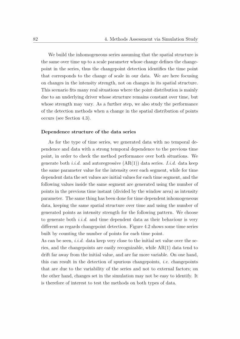
82 4. Methods Assessment via Simulation Study
We build the inhomogeneous series assuming that the spatial structure is
the same over time up to a scale parameter whose change defines the change-
point in the series, thus the changepoint detection identifies the time point
that corresponds to the change of scale in our data. We are here focusing
on changes in the intensity strength, not on changes in its spatial structure.
This scenario fits many real situations where the point distribution is mainly
due to an underlying driver whose structure remains constant over time, but
whose strength may vary. As a further step, we also study the performance
of the detection methods when a change in the spatial distribution of points
occurs (see Section 4.3).
Dependence structure of the data series
As for the type of time series, we generated data with no temporal de-
pendence and data with a strong temporal dependence to the previous time
point, in order to check the method performance over both situations. We
generate both i.i.d. and autoregressive (AR(1)) data series. I.i.d. data keep
the same parameter value for the intensity over each segment, while for time
dependent data the set values are initial values for each time segment, and the
following values inside the same segment are generated using the number of
points in the previous time instant (divided by the window area) as intensity
parameter. The same thing has been done for time dependent inhomogeneous
data, keeping the same spatial structure over time and using the number of
generated points as intensity strength for the following pattern. We choose
to generate both i.i.d. and time dependent data as their behaviour is very
different as regards changepoint detection. Figure 4.2 shows some time series
built by counting the number of points for each time point.
As can be seen, i.i.d. data keep very close to the initial set value over the se-
ries, and the changepoints are easily recognizable, while AR(1) data tend to
drift far away from the initial value, and are far more variable. On one hand,
this can result in the detection of spurious changepoints, i.e. changepoints
that are due to the variability of the series and not to external factors; on
the other hand, changes set in the simulation may not be easy to identify. It
is therefore of interest to test the methods on both types of data.

4.1 Simulation design 83
(a) Iid time series with no change, small change, big change
(b) AR(1) time series with no change, small change, big change
(c) Multiple changepoints, iid and AR(1) time series
Figure 4.2: Simulated time series with zero, one and three changepoints

84 4. Methods Assessment via Simulation Study
Number and magnitude of changepoints
As for the number of changepoints, we start with a single changepoint
with a large magnitude change, the easiest case to detect; we then check
the performance of our methods on a small magnitude change. Besides, we
generate data with three changepoints of varying size and quality (increas-
ing/decreasing intensity strength).
Let λ(j) be the parameter for segment j, where for m changepoints we have
j = 1, . . . ,m + 1. For the single changepoint series, we tried two different
change magnitudes: a big one, from λ(1) = 1 to λ(2) = 2, and a small one,
from λ(1) = 1 to λ(2) = 1.2. Given the window area, λ = 1 produces pat-
terns with an expected number of points equal to 100, λ = 1.2 generates 120
points and λ = 2 generates 200 points on average. Bigger changes have been
tested and lead to analogous conclusions as λ(2) = 2. As for the multiple
changepoint series, we set two positive changes and a negative one, all with
different magnitudes: the segment intensity values are λ(1) = 1, λ(2) = 1.4,
λ(3) = 2.3 and λ(4) = 2. Figure 4.3 shows data with multiple changes.
(a) Homogeneous pattern, 3 changepoints, 4 data segments
(b) Inhomogeneous pattern, 3 changepoints, 4 data segments
Figure 4.3: Examples of data segments patterns for series with multiple
changepoints

4.1 Simulation design 85
The last change is extremely small, to further test the performance of the
detection methods. Each one of these time series was replicated 100 times.
For the inhomogeneous models, the same values are used for Λ. Once all the
time series are generated, we fit the four models described in Section 3.2.2
on all of them and try to detect changepoints with both methods described
in Section 3.2.4. All model fitting is done using INLA.
4.1.3 Single changepoint data generation
As for the homogeneous models (Models 3.2.1 and 3.2.2), data are gen-
erated from a stationary Poisson process, with an initial intensity value of
λ = 1. Data generated under H0 keep the same value for λ all throughout
the series; data generated under H1 have a change in the intensity value in
t = 24, the fixed changepoint. Since the intensity function is constant within
segments, in a homogeneous process λ(j) is the single parameter value for
the intensity at time segment j; for 1 changepoint we have j = 1, 2. In all
replicates λ(1) = 1, while in one scenario λ(2) = 2 and in the other one
λ(2) = 1.2.
As for the non uniform case, data were generated from a spatially inhomo-
geneous function, whose structure is constant over time up to a scale factor,
using an inhomogeneous Poisson process (this is analogous to generating
from a LGCP, but fixing the latent field). Let now λ(j, s) be the value for
the intensity of time segment j at location s, and Λ(j) =∑
s λ(j, s) be the
overall value for the observation window in segment j. Here too, the initial
setting for the intensity function Λ(1) = 1 produced patterns with 100 points
on average over the window, and for alternative data from t = 24 on there
have been again two change magnitude possibilities: λ(2, s) = 2λ(1, s) or
λ(2, s) = 1.2λ(1, s), resulting in Λ(2) = 2 and an expected number of points
equal to 200, or Λ(2) = 1.2 and an expected number of points equal to 120.
Under these conditions, both i.i.d. and AR(1) data were generated.

86 4. Methods Assessment via Simulation Study
Therefore, for i.i.d. homogeneous patterns
H0
{Yt ∼ Poi(1) for t = 1, . . . , 50
H1
{Yt ∼ Poi(1) for t ≤ 24
Yt ∼ Poi(λ(2)) for t > 24
where λ(2) ∈ {1.2, 2}.
For AR(1) homogeneous patterns, let λ(t) = N(Xt)|W | be the maximum
likelihood (ML) estimate for the intensity of the process at time t, where
N(Xt) is the number of points of the pattern, and |W | = 100 is the window
area.
H0
{Yt ∼ Poi(1) for t = 1
Yt ∼ Poi(λ(t− 1)) for t = 2, . . . , 50
H1
Yt ∼ Poi(1) for t = 1
Yt ∼ Poi(λ(t− 1)) for t = 2, . . . , 24
Yt ∼ Poi(λ(2)) for t = 25
Yt ∼ Poi(λ(t− 1)) for t = 26, . . . , 50
For i.i.d. inhomogeneous patterns
H0
{Yts ∼ Poi(λ(1, s)) for t = 1, . . . , 50, s = 1, . . . , 400
H1
{Yts ∼ Poi(λ(1, s)) for t ≤ 24, s = 1, . . . , 400
Yts ∼ Poi(λ(2, s)) for t > 24, s = 1, . . . , 400
where λ(2, s) ∈ {1.2λ(1, s), 2λ(1, s)}.
For AR(1) inhomogeneous patterns, now let λ(t, s) = N(Xts)|C| be the
ML estimate for the intensity of the process at time t in cell s, where N(Xts)
is the number of points at time t inside cell s, and |C| = |W |S
is the (time

4.1 Simulation design 87
invariant) cell area.
H0
{Yts ∼ Poi(λ(1, s)) for t = 1, s = 1, . . . , 400
Yts ∼ Poi(λ(t− 1, s)) for t = 2, . . . , 50, s = 1, . . . , 400
H1
Yts ∼ Poi(λ(1, s)) for t = 1, s = 1, . . . , 400
Yts ∼ Poi(λ(t− 1, s)) for t = 2, . . . , 24, s = 1, . . . , 400
Yts ∼ Poi(λ(2, s)) for t = 25, s = 1, . . . , 400
Yts ∼ Poi(λ(t− 1, s)) for t = 26, . . . , 50, s = 1, . . . , 400
An example of homogeneous and inhomogeneous data can be again found in
Figure 4.1 and Figure 4.2.
4.1.4 Multiple changepoint data generation
For the multiple changepoint analysis, data are generated using the same
methods as the single changepoint data: homogeneous and inhomogeneous
process, i.i.d. and AR(1) time series. There is no difference with regard to a
single changepoint search in H0 data, while H1 data have three changepoints
instead of one. For both homogeneous and inhomogeneous data, change-
points are set at t = 15, 30, 40. In a general inhomogeneous process, with
M = 3 changepoints λ(j, s) is now defined for j = 1, . . . , 4. Following the
fixed values, the expected number of points at every time point is 100 for
segment 1 (Λ(1) = 1), 140 for segment 2 (Λ(2) = 1.4), 230 for segment 3
(Λ(3) = 2.3) and 200 for segment 4 (Λ(4) = 2); they are randomly scattered
in a homogeneous dataset, and randomly distributed given the intensity at
each location for a inhomogeneous dataset. The same technique as in Section
4.1.3 is used for generating time dependent data.
For i.i.d. homogeneous patterns
H0
{Yt ∼ Poi(1) for t = 1, . . . , 50
H1
Yt ∼ Poi(1) for t ≤ 15
Yt ∼ Poi(1.4) for 15 < t ≤ 30
Yt ∼ Poi(2.3) for 30 < t ≤ 40
Yt ∼ Poi(2) for 40 < t ≤ 50
′

88 4. Methods Assessment via Simulation Study
For AR(1) homogeneous patterns
H0
{Yt ∼ Poi(1) for t = 1
Yt ∼ Poi(λ(t− 1)) for t = 2, . . . , 50
H1
Yt ∼ Poi(1) for t = 1
Yt ∼ Poi(λ(t− 1)) for t = 2, . . . , 15
Yt ∼ Poi(1.4) for t = 16
Yt ∼ Poi(λ(t− 1)) for t = 17, . . . , 30
Yt ∼ Poi(2.3) for t = 31
Yt ∼ Poi(λ(t− 1)) for t = 32, . . . , 40
Yt ∼ Poi(2) for t = 41
Yt ∼ Poi(λ(t− 1)) for t = 42, . . . , 50
.
For i.i.d. inhomogeneous patterns
H0
{Yts ∼ Poi(λ(1, s)) for t = 1, . . . , 50, s = 1, . . . , 400
H1
Yts ∼ Poi(λ(1, s)) for t ≤ 15, s = 1, . . . , 400
Yts ∼ Poi(1.4λ(1, s)) for 15 < t ≤ 30, s = 1, . . . , 400
Yts ∼ Poi(2.3λ(1, s)) for 30 < t ≤ 40, s = 1, . . . , 400
Yts ∼ Poi(2λ(1, s)) for 40 < t ≤ 50, s = 1, . . . , 400
.
For AR(1) inhomogeneous patterns
H0
{Yts ∼ Poi(λ(1, s)) for t = 1, s = 1, . . . , 400
Yts ∼ Poi(λ(t− 1, s)) for t = 2, . . . , 50, s = 1, . . . , 400

4.1 Simulation design 89
H1
Yts ∼ Poi(λ(1, s)) for t = 1, s = 1, . . . , 400
Yts ∼ Poi(λ(t− 1, s)) for t = 2, . . . , 15, s = 1, . . . , 400
Yts ∼ Poi(1.4λ(1, s)) for t = 16, s = 1, . . . , 400
Yts ∼ Poi(λ(t− 1, s)) for t = 17, . . . , 30, s = 1, . . . , 400
Yts ∼ Poi(2.3λ(1, s)) for t = 31, s = 1, . . . , 400
Yts ∼ Poi(λ(t− 1, s)) for t = 32, . . . , 40, s = 1, . . . , 400
Yts ∼ Poi(2λ(1, s)) for t = 41, s = 1, . . . , 400
Yts ∼ Poi(λ(t− 1, s)) for t = 42, . . . , 50, s = 1, . . . , 400
An example of both homogeneous and inhomogeneous data series with mul-
tiple changes is in Figure 4.3.
4.1.5 Simulation models and methods
We use the simulated data to run all four model scenarios described in
Section 3.2.2: a simple one assuming a spatially homogeneous process and
introducing a fixed effect to describe the intensity level over time (Model 1,
Formula 3.2.1), a model adding a temporal random effect (Model 2, Formula
3.2.2), a model including an intercept, spatial dependence and heterogeneity
(Model 3, Formula 3.2.3), and finally a more complex model for spatially
inhomogeneous intensity with two smooth effects allowing for both spatial
and temporal dependence within segments (Model 4, Formula 3.2.4).
Since the window is discretized into 400 cells and we have 50 time points,
for each scenario and under each hypothesis the response vector is Y (50 ×400)× 1 = 20, 000× 1.
Models are fitted separately to different parts of the data, according to the
hypotheses. Under the null hypothesis, each model is fitted to the whole
data vector to obtain the marginal data log-likelihood. Under the alternative
hypothesis, for a single changepoint search we
1. choose a minimum segment length of d = 4 to make the changepoint
search more effective and improve the INLA algorithm performance
(see Section 3.2.3)
2. run each model T − 2d + 1 times for each simulation replicate; in
each run, we condition on the changepoint occurring at a location

90 4. Methods Assessment via Simulation Study
τ ∈ {4, 6, . . . , 44, 46} (remember that τ marks the end of a segment)
and fit the considered model to every data segment using INLA; for ev-
ery τ , we obtain two log-likelihood values q1(τ) and q2(τ) (see Section
3.2.4)
3. sum q1(τ) and q2(τ) to obtain the marginal data log-likelihood under
a specific changepoint l1(τ)
4. since we do the same for every possible τ , for every single replicate we
obtain T − 2d+ 1 marginal log-likelihood values under the alternative
hypothesis of one changepoint; they all refer to the whole data series
Y , but they are conditional on different positions for the potential
changepoint
5. use the log-likelihood vector to build the posterior distribution of the
potential changepoint positions for a specific replicate as explained in
Chapter 3
6. for every model, we do the same over 100 data series replicates, thus
we have 100 posterior curves
7. for every curve, we use one of the methods described in Section 3.2.4
to take decisions on the occurrence of a changepoint
8. evaluate the performance of each detection method, for each scenario,
by summarising the results over 100 posterior curves.
For a multiple changepoint search, we can follow either an iterative or a
simultaneous technique, as introduced in Section 3.3. If we use a binary
segmentation algorithm, the same procedure is repeated at every step for
the multiple changepoint detection; we set the algorithm to find maximum
4 changepoints, but different maxima can easily be fixed. When we run
a simultaneous changepoint search, we follow what explained in Chapter
3: we first obtain a few data likelihoods conditional on different numbers of
changepoints and choose the number of changepoints that corresponds to the
highest likelihood; then, we infer the position of every single changepoint via
conditional posterior distributions of every changepoint given the previous

4.2 Simulation results 91
one, the data and the chosen number of changepoints.
We use all detection methods proposed in Chapter 3 in order to assess their
performance and choose the most suitable one(s) for the analysis on real data
presented in Chapter 5.
4.2 Simulation results
After running all the analyses, we obtain results for each of the cases
listed in Section 4.1.1, and we show a few graphs:
• a histogram showing the probability of committing type I errors for H0
data and type II errors for H1 data
• a histogram of the number of changepoints found, where the mode is
chosen as the correct number of changepoints
• a posterior probability plot: conditioning on the chosen number of
changepoints, we obtain the averaged (over 100 replicates) pointwise
posterior probability for each time point to be a changepoint
• an estimate for the intensity function for each time segment produced
by the INLA algorithm, together with a few synthetic measures and a
comparison with the true values.
As for Section 4.1, a summarised overview of the results with general com-
ments is given first in Section 4.2.1; detailed comments can be found in the
following Sections. A few representative results are displayed in figures along
the Chapter. For all the remaining results, we refer to figures in the Ap-
pendix. As a note, data without changepoints are labelled as H0, single
big change data as H1b and single small change data as H1s in all graphs;
multiple changepoint data are simply labelled as H1.
4.2.1 Summary of the simulation results
The BF (and SIC) and PT methods’ performance was evaluated according
to type I and type II errors, number and position of detected changepoints
and values of the intensity estimates.

92 4. Methods Assessment via Simulation Study
Type I and II errors
A summary of the methods performance is in Table 4.2.
Table 4.2: Significance levels (H0 data) and power levels (H1 data)
Homogeneous data Inhomogeneous data
Model 1 Model 2 Model 3 Model 4
BF PT BF PT BF PT BF PT
IID
H0 λ = 1 0 ≤ 0.05 0 ≤ 0.05 0 ≤ 0.1 0 ≤ 0.01
H1
λ2 = 2 1 1 1 1 1 1 0 1
λ2 = 1.2 1 1 1 0.98 0 0.34 0 0.3
mult BinSeg 1 1 0.99 1 0 0.93 0 0.26
mult Simult 1 1 0 0
AR(1)
H0 λ = 1 0.96 0.66 0.38 0.24 0.15 0.26 0 0.18
H1
λ2 = 2 1 0.97 0.81 0.75 0.53 0.81 0 0.52
λ2 = 1.2 1 0.73 0.43 0.36 0.19 0.54 0 0.37
mult BinSeg 1 0.98 0.94 0.91 0.55 0.84 0 0.67
mult Simult 1 1 0 0
In general, the Bayes Factor method (and, analogously, the simultaneous
approach) performs very well as regards the first two models: in most cases
type I errors are very small (with the exception of one case with time depen-
dent data, but we expect poorer performance on these data, for the reasons
introduced in Section 3.1) and type II errors are negligible in all cases. When
we fit more complicated models including a spatial effect, though, the per-
formance is very poor: the method is too conservative and does not detect
changepoints, irrespective of their magnitude.
The Posterior Threshold method gives a better performance over all models;
this is sensible, as the threshold value can be tuned according to the model.
A few ’grey’ zones are produced, but the overall conclusions are correct in
most cases, and there is at least some ability to detect changes in all situa-
tions (unlike the Bayes Factor method).
A further summary of this performance can be found in Table 4.3: the first
row in each table concerns data generated under H0 and the second row con-
cerns data generated under H1, therefore numbers have to sum to 100 by row.
It is very plain that the PT method has a better overall performance: as re-
gards null data (first row), the behaviour of the two methods is very similar,

4.2 Simulation results 93
but the PT method is 20 percentage points better in finding changepoints in
H1 data (second row).
Table 4.3: Summary of type I and type II errors
H0 correct result False positive
False negative H1 correct result
BF method ( %) PT method ( %)
81.38 18.63 79.75 20.25
43.79 56.21 23.92 76.08
Number and location of changepoints
As for the number of detected changepoints, results are linked, but not
necessarily identical, to the previous ones: committing or not a type II error
only concerns the rejection of H0 and tells nothing on the number and posi-
tions of the detected changepoints, which is of special interest in a multiple
changepoint search. Table 4.4 shows a summary of the results.
We can see that as far as H0 data are concerned, results are correct in all
cases: even in situation where some changepoints were found, as in AR(1)
data, all the positions were different, and this indicates they are spurious
changepoints and not ’true’ ones. As regards the detection in H1 data, the
BF method suffers from the above mentioned issue: it is very precise in
detecting the true change(s) in the first two models, but too conservative
when spatial dependence and inhomogeneity is introduced. The PT method
performs much better: when changepoints are not detected in the majority
of replicates, it is due to the small magnitude of the change, which means the
method is not too sensible; despite the small size, a percentage of replicates
still had a change detected. The only wrong conclusion concerns the multiple
changepoint i.i.d. data series under the most complicated model; in all other
cases, conclusions are very sensitive and the detected positions are correct
or as close as it makes no difference. It is interesting to note that spurious
changes in time dependent data do not affect conclusions.

94 4. Methods Assessment via Simulation Study
Table 4.4: Position of the detected changepoints
Homogeneous data Inhomogeneous data
Model 1 Model 2 Model 3 Model 4
True BF PT BF PT BF PT BF PT
IID
H0 No chp – – – – – – – –
H1
24 24 24 24 24 24 24 – 24
24 24 24 24 24 – – – –
15 30 40 BinSeg 15
30
40
15
30
40
15
30
40
15
30
40
– 15
30
– –
15 30 40 Simult 28 28 16 – –
AR(1)
H0 No chp – – – – – – – –
H1
24 24 24 24 24 24 24 – 24
24 24 24 – – – 24 – –
15 30 40 BinSeg 15
30
41
15
30
41
15
30
40
15
30
40
15
30
15
30
41
– 15
30
40
15 30 40 Simult 28 13 28 13 40 – –
Intensity estimates
Lastly, a few comments about the intensity estimates, which again depend
on the above presented results. A summary of the estimated values is given
in Table 4.5. Note that the intensity is a inhomogeneous function which takes
different values over space. In this table, for brevity reasons, only the mean
value is reported, but the mean range (over the replicates) and credibility
bands are also available as in every Bayesian inference output. Given the
detected changepoints, estimates are very accurate over all the simulated
scenarios: when a changepoint is not detected, values are an average between
the two segments’ true values, and when a changepoint is only detected
in part of the replicates (as it happens with very small changes), the true
magnitude of the change is shrunk. In all cases the correct (increasing or
decreasing) trend is captured.

4.2 Simulation results 95
Table 4.5: Estimates for the segment intensity
Homogeneous data Inhomogeneous data
Model 1 Model 2 Model 3 Model 4
True intensity BF PT BF PT BF PT BF PT
IID
H0 1.00 1.00 1.01 1.00 1.01 0.99 1.00 1.00 1.00
H1
1.00 2.00 0.99
2.00
1.04
2.00
1.00
2.00
1.04
2.00
0.99
2.00
1.00
2.00
1.50 1.00
2.00
1.00 1.20 1.00
1.20
1.01
1.20
1.00
1.20
1.01
1.20
1.09 1.10 1.10 1.10
1.00 1.40 2.30 2.00 1.00
1.40
2.17
2.07
1.00
1.38
2.22
2.05
1.01
1.40
2.12
2.10
1.00
1.38
2.15
2.08
1.58 1.20
1.50
2.20
1.51 1.60
AR(1)
H0 1.00 0.99 1.01 0.96 0.99 0.92 0.98 0.87 0.98
H1
1.00 2.00 1.05
2.04
1.05
2.03
1.09
2.10
1.11
2.05
1.18
1.90
1.08
1.99
1.41 1.20
1.78
1.00 1.20 1.01
1.14
1.01
1.14
1.06 1.06 1.10 1.01
1.18
1.07 1.09
1.00 1.40 2.30 2.00 1.02
1.40
2.21
1.08
1.02
1.40
2.22
2.07
1.05
1.39
2.15
2.02
1.07
1.38
2.14
2.04
1.12
1.40
2.13
1.10
1.42
2.18
2.08
– 1.15
1.41
2.03
1.97
In the next Sections, detailed comments about the simulation results
are presented, along with some representative graphs; a complete list of the
figures is in Appendix A.
4.2.2 Single changepoint detection with Bayes Factor
method
In this Section, we summarise results for a single changepoint search on
both i.i.d. and time dependent data. Bayes Factor (BF) and SIC method
(SIC) perform extremely similarly; the SIC method tends to be ever so
slightly less conservative, but the difference is negligible in most cases, and
never substantial. We will therefore not explicitly report results for the SIC

96 4. Methods Assessment via Simulation Study
method.
As we say in Section 3.2.4, the Formula (3.2.8) we apply to simulated data
is a conservative version of the commonly used Bayes Factor. This is for two
main reasons: first of all, a positive but small value for the Bayes Factor is
usually interpreted as ’small evidence’, and we would like to protect results
against type I errors. Secondly, as log-likelihoods are returned by the INLA
algorithm, when computing the sum in the numerator of the Bayes Factor
exponents have to be taken and issues due to software numerical rounding
raise, as number easily go to infinity or 0. The version in Equation 3.2.8 is
instead perfectly computable with no need to convert logarithms.
On both i.i.d. and time dependent data, the BF method performs very well
over three of the four model scenarios as regards detection and location of
the change.
Homogeneous models
In the fixed and temporal effect models the statistic correctly rejects H0
in all i.i.d. replicates, even when a very small change occurs; moreover, the
detected changepoint position is correct in all replicates with a big change,
and in most with a small change (very close in the remaining ones). The
estimated values produced by INLA are compactly distributed around the
true value, and both their mean and median are a good choice for the in-
tensity parameter posterior estimate, being always less than 0.05 away from
the correct values. An example of the simulation output is in Figure 4.4.
Predictably, results are not so neat on time dependent data, and the main
cause is data variability that will lead to the detection of changepoints that
have not been set a priori in H0 data; nevertheless, introducing the temporal
effect in the model has a high positive effect on the statistic performance on
null data, as the mode of the detected number of changepoints is correctly
set to 0. For both models, the performance is very good for data generated
under the alternative hypothesis as regards both power and location. As
for the estimated values, the variability among the replicates is much higher
than the i.i.d. data one, still both mean and median are very close enough
to the initial intensity values. Some results for AR(1) data are in Figure 4.5.

4.2 Simulation results 97
Figure 4.4: Single changepoint search on iid data, with the fixed effect model
and the BF method
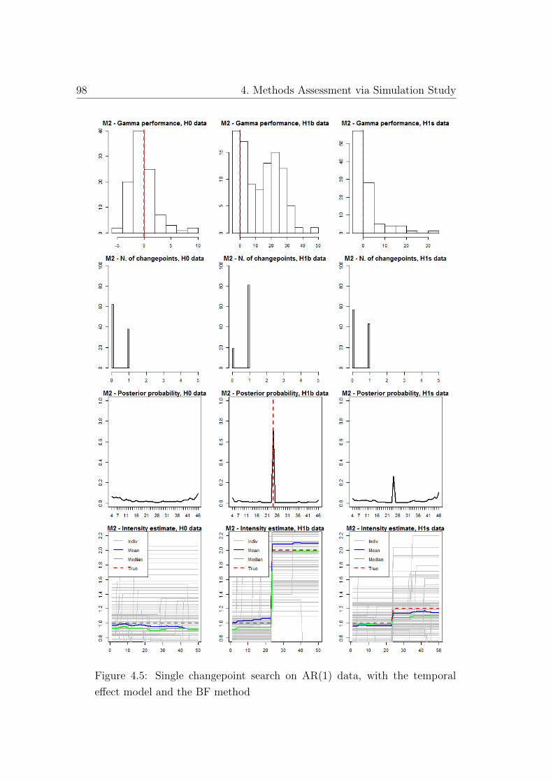
98 4. Methods Assessment via Simulation Study
Figure 4.5: Single changepoint search on AR(1) data, with the temporal
effect model and the BF method

4.2 Simulation results 99
Inhomogeneous models
The third and fourth models allow for spatially inhomogeneous intensity
functions and a spatial random effect, and are therefore applied to data
generated following an inhomogeneous process. An example of the resulting
graphs is in Figure 4.6.
Figure 4.6: Single changepoint search on iid data, with the spatio-temporal
effect model and the BF method - Power level and location of the changepoint

100 4. Methods Assessment via Simulation Study
The significance level is correctly set to 0 over all replicates for both
models, but a conservatism issue raises here, as the big change is the only
one detected (in the correct location) with the spatial model, while with the
spatio-temporal model no change is detected over all the data series, despite
high peaks corresponding to t = 24 in all posterior distributions. The most
interesting novelty with inhomogeneous models is the intensity estimate: we
obtain a value for every grid cell, hence the estimate is shown as a pixel
image where for every cell values are averaged over the corresponding time
segment (we choose the mean as synthetic value, and the median would
lead to extremely similar results in all cases). In all cases (both spatial and
spatio-temporal model, and both i.i.d. and AR(1) data) the estimates are
very accurate given the detected changepoints: they not only capture the true
range of values very well, but also produce a smooth image that correctly
estimates the spatial trend. When changepoints are not detected, the range
of the estimated values is correctly set in between the two segment’s values
(see e.g. Figure 4.7). In AR(1) data, some small drifts with respect to the
set values occur, due to the strong time dependency and variability in the
data.

4.2 Simulation results 101
Figure 4.7: Single changepoint search on iid data, with the spatio-temporal
effect model and the BF method - Estimated intensities

102 4. Methods Assessment via Simulation Study
4.2.3 Single changepoint detection with Posterior
Threshold method
The method consisting in fixing a threshold for posterior probability val-
ues can be adapted to the model, in order to be able to recognise changepoints
even when spatial and/or temporal dependence are considered and lead to
higher data variability, e.g. by raising the threshold with respect to a simpler
model. Having simulated data, we bound the choice of the threshold to a
certain significance level, giving an objective threshold value that will still
depend on the model applied to our data.
We use a threshold corresponding to α ≤ 0.05 for the fixed and temporal
effect models, and one corresponding to α ≤ 0.1 for the spatial and spatio-
temporal inhomogeneous models. The different choice for α is due to the
fitted model: for the inhomogeneous models, fixing a lower α would result in
a threshold equal to 1, which is not a sensible choice. For dependent data,
fixing a threshold based on the significance level obtained on such variable
data is tricky. We decide to fix the threshold referring to i.i.d. data, keeping,
where possible, a stricter criterion: this results in a choice of α ≤ 0.01 for
the two homogeneous models and in α ≤ 0.1 for the inhomogeneous ones for
the same reasons explained above.
The performance of this method on a single changepoint search is, in general,
preferable to the BF method on alternative data.
Homogeneous models
The threshold for these two models for i.i.d. data is 0.2 with the fixed
effect model and 0.25 for the temporal model; for time dependent data, it
is 0.55 with the fixed effect model and 0.65 for the temporal model. A
significance level not greater than 0.05 is set on i.i.d. data; on AR(1) data,
it is higher and, as for the BF method, leads to an overall wrong conclusion
with a fixed model but a correct conclusion when the temporal effect is
introduced; the significance level is anyway much better on time dependent
data than the one obtained by the BF method.
As for i.i.d. data, the changepoint is correctly detected and the right location
is identified as with the BF method, since the choice of the method only

4.2 Simulation results 103
concerns the number of changepoints, while the correct location is given by
the posterior probability distributions, irrespective of the method used. The
same conclusions concern the intensity estimate. A summary of the results
is in Figure 4.8.
As far as time dependent data are concerned, no evidence for a specific change
is shown by the H0 data posterior distribution, while conclusions regarding
both number and location of changepoints are correct in most H1b data and
not significant in H1s data. As said in the BF method results, single replicate
estimates are extremely variable, still both mean and median perform well as
estimates for λ. In H1s data, there is a small underestimation of the second
segment value, due to the difficulty in detecting the small change. Results
for the fixed effect model are in Figure 4.9.

104 4. Methods Assessment via Simulation Study
Figure 4.8: Single changepoint search on iid data, with the fixed effect model
and the PT method

4.2 Simulation results 105
Figure 4.9: Single changepoint search on AR(1) data, with the fixed effect
model and the PT method

106 4. Methods Assessment via Simulation Study
Inhomogeneous models
The threshold for the inhomogeneous models is 0.95 for all data, corre-
sponding to a significance level not greater than 0.1 on i.i.d. data and low
enough to reach the overall correct conclusion on AR(1) data.
Figure 4.10: Single changepoint search on AR(1) data, with the spatial effect
model and the PT method - Power level and location of the changepoint

4.2 Simulation results 107
The most important comparison to the BF method conclusions con-
cern data with a changepoint; with the spatial model results are similar
on i.i.d. data: one changepoint in H1b data, no changepoint in H1s data.
On time dependent data, though, a changepoint is correctly detected even
when it has a small magnitude with the spatial model. The spatio-temporal
model also leads to better conclusion as the big change is detected on both
i.i.d. and time dependent data. See Figure 4.10 for a summary of the re-
sults.
Again, location estimates are correct and the intensity estimates are very
accurate given the changepoint locations and the variability in the data, as
shown in Figure 4.11. When the changepoint is not detected in a consistent
part of the replicates, its actual size will be shrunk in the estimates.

108 4. Methods Assessment via Simulation Study
Figure 4.11: Single changepoint search on AR(1) data, with the spatial effect
model and the PT method - Estimated intensities

4.2 Simulation results 109
4.2.4 Iterative multiple changepoint detection
with Bayes Factor method
When applied to a multiple changepoint search, the BF method performs
more poorly than in the single changepoint case: its results are good for the
first two homogeneous models, but not for the inhomogeneous ones. The
greater difficulty in detecting changepoints in more complex models in this
analysis can also be imputed to the very small change magnitudes that have
been set over these datasets. It is interesting to notice that the range of γ
values is in all cases very consistent: either nearly all values are negative or
they are positive, the power level is 1 or 0, there is no grey zone. Perhaps,
as the posterior threshold is tuned according to the fitted model, the γ′τ∗
statistic (Formula 3.2.8) decision threshold should also be changed according
to the model. There is anyway no reference we are aware of about giving
a different threshold than zero to the logarithm of the Bayes Factor. As
the method does not perform well on time dependent data, we only use the
Posterior Threshold method on those ones.
The significance level is of course very similar to the single changepoint results
over all data, as it only concerns the rejection of H0. Moreover we already
know the INLA estimates are very good given the detected changepoints.
What is of interest here is then the actual number of detected changepoints
and their location. for every model. Remember that with multiple changes
we only have one type of data generated under H1.
As for the fixed effect model, 3 changepoints were correctly found in 15,
30 and 40. The peak in 40 is smaller as this changepoint has the lowest
change magnitude along with the highest data variability (from λ = 2.3 to
λ = 2). Consistently, the INLA estimate are very accurate in the first two
segments, and then a bit lower than 2.3 on the third and a bit higher than
2 in the fourth, shrinking the actual magnitude for the last changepoint.
Nevertheless, the general behaviour of the intensity function is very well
captured.
Introducing a temporal effect on i.i.d. generated data does not substantially
modify the results with respect to the first model, except it flattens the
third peak in 40 even more, even if this time point will still be detected.

110 4. Methods Assessment via Simulation Study
In the INLA estimates it is of interest to see that the abruptness of all
steps is softened, giving more gradual changes, and that best suits real data
situations.
When moving on to inhomogeneous processes, problems in the BF method
begin, as no changepoints are identified in any data series. Since the first
potential changepoint found (the one returning the maximum log-likelihood
value) is considered non significant, the binary segmentation algorithm stops
running; nevertheless, the posterior distribution curve shows a very high peak
at position t = 30, where the change with the largest magnitude is set. Due
to the lack of changepoint detections, the estimate images are very precise
for H0 data, but the range of values for H1 data has a mean of 1.7, which is
a good average across all segments.
All figures can be found in Appendix A.
4.2.5 Iterative multiple changepoint detection
with Posterior Threshold method
We finally fit the four models on both i.i.d. and AR(1) data, looking
for multiple changepoints in the series and making decisions based on the
posterior probability distribution and a fixed threshold. On i.i.d. data, we
detect different possibilities for the threshold corresponding to a probability
of committing the type I error equal to 0.01, 0.05, 0.1, when possible. Then,
for i.i.d. data when homogeneous models are fitted, we choose the threshold
corresponding to α = 0.05. In the two inhomogeneous models, the only
sensible threshold corresponds to α = 0.1 as lower values for α would result
in a threshold equal to 1. For the same reason, the threshold is maintained at
the same value for AR(1) data, while in the homogeneous models we choose
a stricter threshold, corresponding to α = 0.01 on i.i.d. data, as it is much
more likely to detect changepoints even in H0 data series when data are time
dependent.

4.2 Simulation results 111
Homogeneous models
The threshold for the first model is 0.25 for i.i.d. data and 0.45 for AR(1)
data; for the second model, it is the same for i.i.d. data and 0.4 for AR(1)
series.
Conclusions concerning the detection of multiple changes are very good: the
two greatest changes in t = 15 and t = 30 are detected over all cases, and
the small one in t = 40 is still detected on all data series, except for the
AR(1) data with the temporal model, where most likely the data variability
together with the inclusion of a time dependence hides the small change. As
for the location, the only conclusion that is slightly wrong concerns the last
small change that is sometimes detected in t = 41 instead, but in the greatest
majority of practical studies, this result will be considered precise enough to
make correct description and inference on the phenomenon under study.
The estimated stepwise function for the intensity is a little smoothed at
the step angles, but very close to the true one. Even on time dependent
data, despite the variability of the estimates, a stepwise process is identifiable
through the series, across all replicates, and the synthetic measure chosen for
estimation are both performing well.
An output example is in Figure 4.12.

112 4. Methods Assessment via Simulation Study
Figure 4.12: Multiple changepoint search on AR(1) data, with the temporal
effect model and the PT method

4.2 Simulation results 113
Inhomogeneous models
As for the single search, the threshold is 0.95 for all data and the spatial
model, and 0.9 for the spatio-temporal model.
As for the spatial model, on i.i.d. data the number of changepoints is un-
derestimated, as the mode is 2; a third non significant peak corresponds to
t = 40. In AR(1) H0 data, correct overall conclusions are drawn; on H1 data
the mode for the number of changes is 3, and all three peaks in the poste-
rior distribution correspond to the correct locations. As for the estimated
images, the spatial trend is correct over all segments, the range is a little
overestimated over the first two segments and then, as usual, the estimated
distance between third and fourth segment is smaller than the true one.
When fitting the last model on i.i.d. data the power, is much lower, there-
fore the main decision is not to reject H0. The second option would be to
have 2 changepoints, correctly identified in the posterior distribution by two
peaks at 15 and 30, nevertheless they are not considered significant in the
majority of cases. The estimate is therefore a single image, with the correct
spatial trend and a mean value close to 1.6, a good average of the four time
segments. Time dependent data show sensibly better results, as the model
suits them better: a correct conclusion of no changepoints is drawn in H0
data, and the mode of the number of changepoint is now correctly situated
at 3 for H1 data, where the three peaks in the posterior correspond to the
true changes in 15, 30, 40. Therefore the conclusion is overall correct despite
the strong time dependence, when using a high strict threshold and account-
ing for both spatial and temporal dependence within segments. Again, the
estimated images produce a good imitation of the set values. An example
figure is in Figure 4.13 and 4.14.

114 4. Methods Assessment via Simulation Study
Figure 4.13: Multiple changepoint search on AR(1) data, with the spatio-
temporal effect model and the PT method - Power level and location of the
changepoint
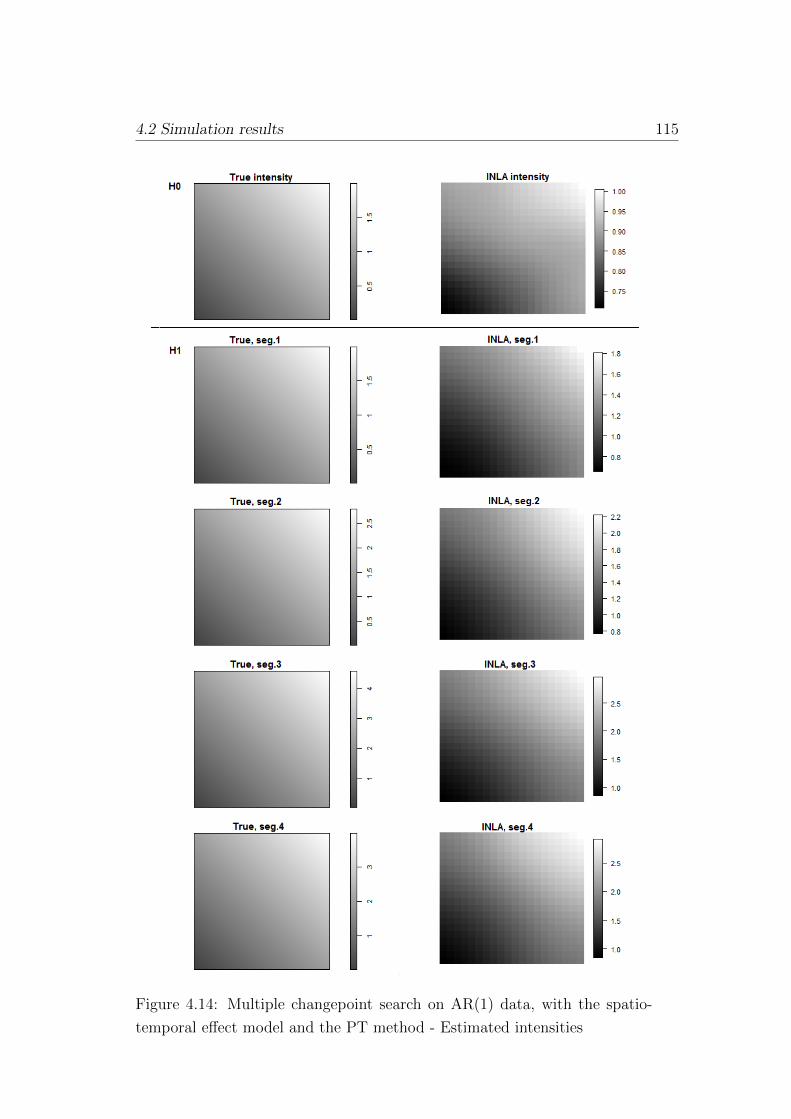
4.2 Simulation results 115
Figure 4.14: Multiple changepoint search on AR(1) data, with the spatio-
temporal effect model and the PT method - Estimated intensities

116 4. Methods Assessment via Simulation Study
4.2.6 Simultaneous multiple changepoint detection
Results have been presented so far that concern both a single and a mul-
tiple unknown changepoint search; therefore, they cover a wide range of
changepoint questions. Additional information on our methods’ performance
would derive from a comparison of the iterative algorithms to a simultaneous
detection approach.
In this study, we are particularly interested in understanding the ability of
the methods to detect changepoints. Therefore, we focus on the results of
the simultaneous search method on H1 data with multiple changes, and we
present a summary of the results regarding the number and locations of de-
tected changes. We do not focus on the estimated values, since, as we pointed
out already, they depend on the INLA algorithm and not on the detection
method, and are always very accurate given the changepoints.
As for the changepoint location, with this method it will be only approxi-
mately detected. Indeed, as introduced in Section 3.3.4, computations be-
come relatively intense when all the possible segment likelihoods have to be
computed, therefore we used Reduced Filtering Recursions (RFR). In partic-
ular, we drew a subset of the 50 time points by choosing equispaced points
with an interpoint distance equal to 3. This generated a sample of 17 time
points, namely 1, 4, 7, . . . . Changepoints will be looked for within the sub-
set, therefore their location will not be exact; if the method performs well,
though, it should be very close to some, or all, the set changepoints τ1 = 15,
τ2 = 30, τ3 = 40.
A summary of the detected changes is in Table 4.6 for i.i.d. data and Table
4.7 for AR(1) data.
Table 4.6: Simultaneous search - detected changepoints on iid data
Model No of changepoints Location (no of repl.)
Fixed 1 28 (96/100)
Temporal 1 28 (63/100), 16 (33/100)
Spatial 0 —
Sp-temp 0 —

4.2 Simulation results 117
Table 4.7: Simultaneous search - detected changepoints on AR(1) data
Model No of changepoints Location (no of repl.)
Fixed 1 28 (58/100), 13 (30/100)
Temporal 1 28 (43/100), 13 (33/100), 40 (10/100)
Spatial 0 —
Sp-temp 0 —
As regards i.i.d. data, first of all, we immediately see that the method
shows to be more conservative than the binary segmentation algorithms, as
it detects at most one change over data that actually have three changes. Its
performance is extremely similar to the BF method: one changepoint for the
homogeneous models, no changepoints for the inhomogeneous ones. Indeed,
we have pointed out the relationship with the Bayes Factor in Section 2.3.5.
As for the detected location, results are very sensible. In the fixed model,
the changepoint is identified as very close to t = 30, which is the location
of the change with the largest magnitude (from λ2 = 1.4 to λ3 = 2.3). As
soon as the temporal effect is included, a second possible location is high-
lighted (though only by a minority of replicates) that is the closest point to
the true changepoint location τ1 = 15. The small changepoint in 40 is never
detected. As happened more than once over the simulation study, the spatial
effect and spatio-temporal effect model lead to the detection of no significant
changepoints when combined with the simultaneous approach.
When time dependent data are analysed, there is no change in the conclu-
sions as regards the inhomogeneous models: again, as happens with all the
analyses carried out using the BF method, no changepoint is considered sig-
nificant. Nevertheless, results improve when working with the homogeneous
models. The number of detected changepoints is still 1, but the locations are
more evenly distributed close to the three true changes. The majority of the
locations are close to the change with the largest magnitude, i.e. τ2 = 30,
but there is a consistent percentage of replicates where the second largest
change, τ1 = 15, is (approximately) detected instead, and with the temporal
effect some of the replicates show a changepoint correspondent to the third
one, τ3 = 40. Further comments can be found in Section 4.4.

118 4. Methods Assessment via Simulation Study
4.3 Changes in the spatial structure
We now briefly check the performance of the proposed methods with a
more general inhomogeneous intensity function. As explained in Chapter 1,
we still look for changepoints over time, not over space, but we now aim at
detecting changes not only in the scale of the intensity function, but also in
its spatial structure.
4.3.1 General framework
So far, all the simulated data series are generated by choosing a constant
spatial structure for the intensity function and allowing for a change in scale,
i.e. a changepoint corresponds to a greater or smaller number of points,
which follow the same spatial distribution. We generate such data for two
main reasons: first of all, the real dataset that motivated the work presents a
spatial structure that is roughly constant over time, therefore changes mainly
concern the number of points. Secondly, this scenario represents a step to-
wards the analysis of inhomogeneous processes, without being too general,
and we consider it a good starting point for evaluating the performance of
the proposed methods.
Nevertheless, we would ideally like a methodology that is able to detect any
type of change over time in the intensity function of a inhomogeneous pro-
cess. Hence, we are now interested in relaxing the spatial assumption and
allowing the intensity function to change in space as well as in time, as hap-
pens in many real situations. This might lead to two more different types
of change: a change in structure, when the overall number of points remains
approximately the same but the spatial distribution changes, and a change
in both scale and structure.
We believe our methods to hold over this general situation as well: when
looking for a change with the proposed algorithms, we never specify that we
are looking for a different number of points; we try and split the data at all
different time points and look for the single equation (no changepoint) or
the product of M + 1 equations (M changepoints) that describe the dataset
best, irrespective of the type of change that occurred. Therefore, if we use a

4.3 Changes in the spatial structure 119
model that includes a spatial effect, we expect our methodology to be able
to identify changepoints in both space and time.
4.3.2 Design
We do not replicate the whole complex simulation study we carried out
and reported in this Chapter so far. We only want to test the performance
of our methods in detecting changes in the spatial structure as well as scale
on a restricted scenario. Indeed, for studying this situation we only work on
inhomogeneous i.i.d. data generated under the alternative hypothesis of one
changepoint. The spatially homogeneous case is of no interest here, and if the
method works for a single changepoint search it is straightforward to extend
it to multiple changes with the tools we provide. We use the same values for
T = 50, S = 400 and the same window W , and the changepoint is again set
in the centre of the time series, at t = 24. We cover both the case of only
spatial change and the case of spatial plus scale change. For data presenting
a change in both scale and spatial structure, we use the large magnitude
change, therefore we have 100 data series with Λ(1) = 1 for segment y1:24
and Λ(2) = 2 for segment y25:50. In conclusion, we have
1. Data with only a spatial change
• 100 replicates of data series with T = 50 time points
• 1 changepoint in t = 24
• same overall intensity strength across segments:
Λ(1) =∑
s λ(1, s) = Λ(2) =∑
s λ(2, s) = 1
• different spatial structure
– segment 1: higher values for top-right cells, lower values for
bottom-left cells
– segment 2: higher values for bottom-left cells, lower values for
top-right cells
2. Data with both spatial and scale change
• 100 replicates of data series with T = 50 time points
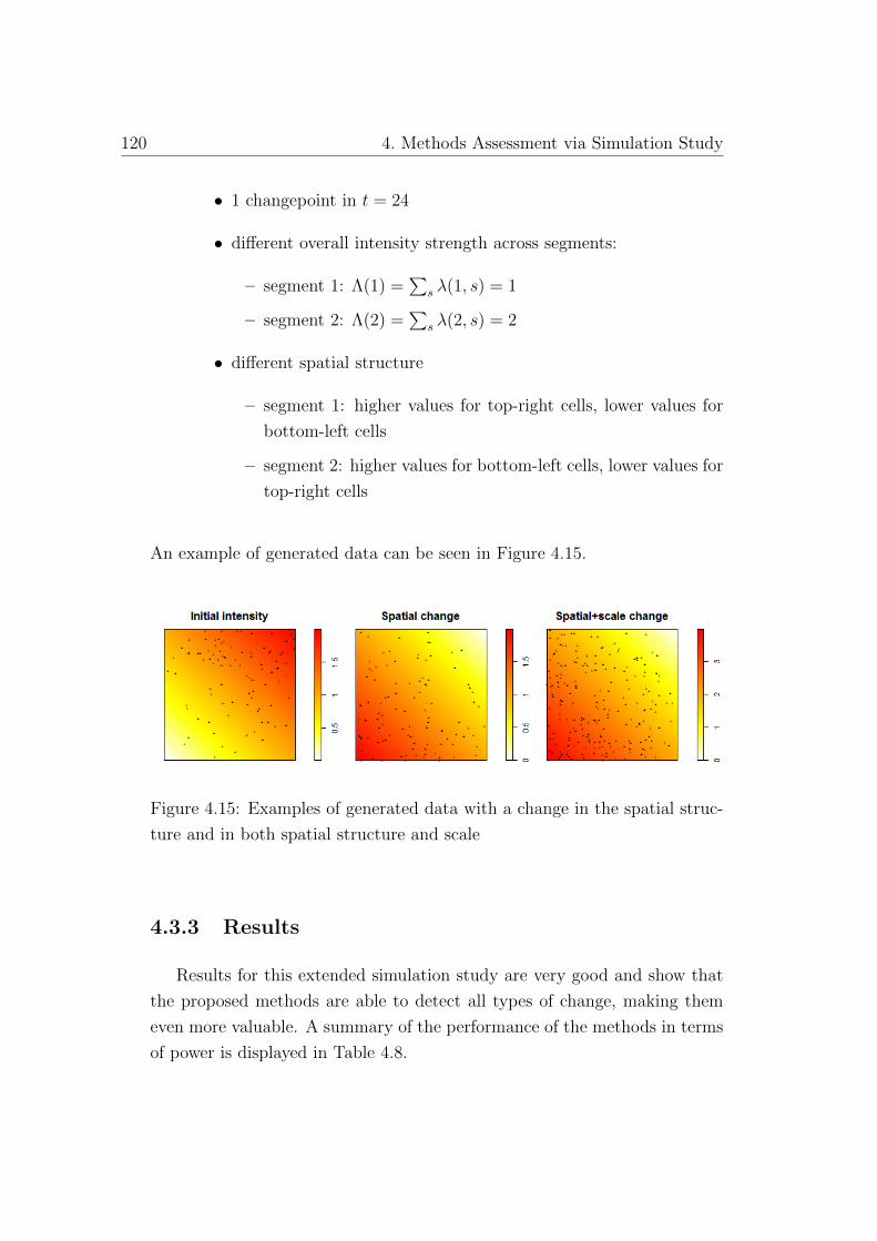
120 4. Methods Assessment via Simulation Study
• 1 changepoint in t = 24
• different overall intensity strength across segments:
– segment 1: Λ(1) =∑
s λ(1, s) = 1
– segment 2: Λ(2) =∑
s λ(2, s) = 2
• different spatial structure
– segment 1: higher values for top-right cells, lower values for
bottom-left cells
– segment 2: higher values for bottom-left cells, lower values for
top-right cells
An example of generated data can be seen in Figure 4.15.
Figure 4.15: Examples of generated data with a change in the spatial struc-
ture and in both spatial structure and scale
4.3.3 Results
Results for this extended simulation study are very good and show that
the proposed methods are able to detect all types of change, making them
even more valuable. A summary of the performance of the methods in terms
of power is displayed in Table 4.8.

4.3 Changes in the spatial structure 121
Table 4.8: Results summary for data with a change in spatial structure
Homogeneous data Inhomogeneous data
Model 1 Model 2 Model 3 Model 4
BF PT BF PT BF PT BF PT
Spatial
Power 0.38 0.44 0.42 0.26 1.00 1.00 1.00 1.00
Location – – – – 24 24 24 24
Estimate 0.95 0.95 0.97 0.97 1.05
1.00
1.03
1.01
1.06
1.02
1.04
1.00
Spatial and scale
Power 1.00 1.00 1.00 1.00 1.00 1.00 1.00 1.00
Location 24 24 24 24 24 24 24 24
Estimate 1.00
1.95
1.00
1.95
0.99
1.96
0.99
1.97
1.06
2.00
1.01
2.00
1.03
2.01
1.02
2.00
Results for the first two models, with fixed and temporal effect, are very
similar for the BF and PT method. An example of the simulation output is
in Figure 4.16 concerning both data with only a change in spatial structure
(labelled as H1sp data) and data with change in scale and structure (labelled
as H1ss) for the fixed model with the PT method; for more (similar) results,
see Appendix A.
As regards data with only a change in the spatial structure, as expected
the first two models do not perform very well in detecting the change, since
the spatial effect is not included and they ignore the inhomogeneity in the
intensity function, i.e. they assume that the intensity function is constant
over space. It is nevertheless interesting to point out that, in the minority of
cases where the changepoint is detected, it is in the correct location t = 24.
For what concerns data with a change in both spatial structure and scale,
the change is correctly detected in all replicates even in the homogeneous
models, as a change in the number of points is recognized as changepoint
over all models.
As soon as spatial inhomogeneity and dependence are included (Models 3
and 4), results show that a changepoint is correctly detected in all replicates
(Figure 4.17 for a representative graph, and the Appendix for more graphs).
The power level is 1, and the location is correctly estimated in all datasets.

122 4. Methods Assessment via Simulation Study
Figure 4.16: Results for a changepoint search on data with a change in the
spatial structure, with the fixed effect model and the PT method

4.3 Changes in the spatial structure 123
Figure 4.17: Changepoint search on data with a change in the spatial struc-
ture, with the spatio-temporal model and the PT method - Power level and
location of the changepoint
As for the intensity estimates (e.g. Figure 4.18), since only a spatial
change takes place, the values for Λ(1) and Λ(2) are extremely similar.
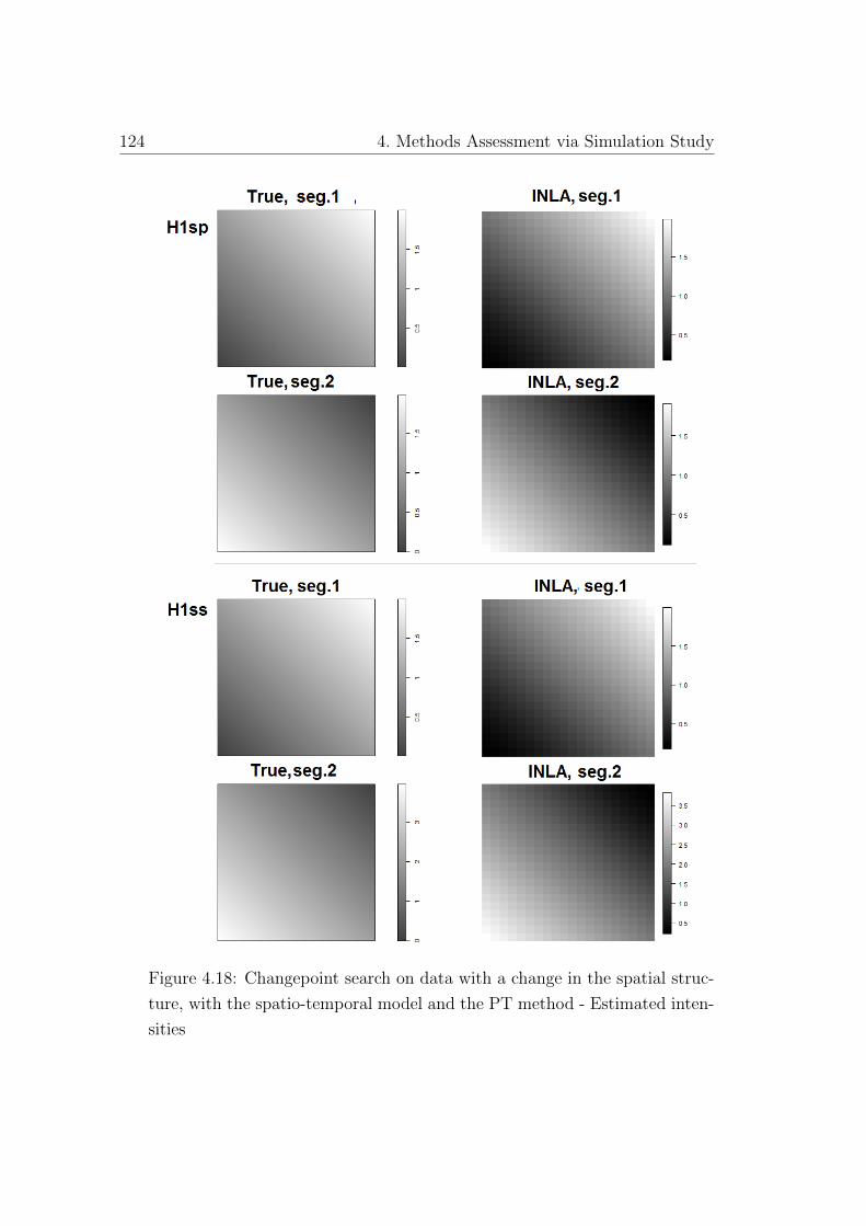
124 4. Methods Assessment via Simulation Study
Figure 4.18: Changepoint search on data with a change in the spatial struc-
ture, with the spatio-temporal model and the PT method - Estimated inten-
sities

4.4 Discussion 125
We can appreciate a slight decrease in the estimated values from segment
1 to segment 2; this happens in all results as the original dataset is the same
(100 replicates of a inhomogeneous process under H1) and must be imputed
to the uncertainty linked to the single process realizations. However, all es-
timates are very close to 1, the initial set value. Over all cases the power is
1, the location is in 24 and the estimated values are close around 1 for the
first time segment and around 2 for the second segment. In particular, the
estimate for the second segment is very precise for the two inhomogeneous
models, while it is slightly underestimated in the first two models, due to the
lack of spatial effects.
There are no substantial differences in the performance of the BF and PT
method; the BF method performs even better than in the only-scale change
situation (previous simulation study), as it does not suffer from too much
conservatism and gives sensibly good results over all models, therefore gen-
eralising the type of change improves the BF method results.
4.4 Discussion
Our simulation study consisted in fitting four different model scenarios
over both i.i.d. and time dependent data, generated with single or multiple
changepoints and with a homogeneous or inhomogeneous intensity function;
100 replicates were produced for each case, over a square observation win-
dow. Once the models were fitted, Bayes Factor, SIC and Posterior Threshold
methods were applied to detect a single changepoint in the process intensity;
as for multiple changes, both some iterative techniques and a simultane-
ous search have been carried out. The first model, including only a fixed
effect, was more suitable for homogeneous i.i.d. series; the temporal effect
model for time dependent homogeneous data; the spatial effect model for
i.i.d. inhomogeneous data; finally, the spatio-temporal model fits the AR(1)
inhomogeneous time series best.

126 4. Methods Assessment via Simulation Study
4.4.1 Methodological discussion
Both the BF and the PT method results coincide with likelihood-based
results if we choose non informative priors in all cases; the likelihood for each
potential changepoint position is then rescaled so that the final distribution
integrates to one and is a proper posterior distribution. However, they show
two advantages with respect to likelihood-based methods: first of all, they
can be extended to any prior setting and exploit external knowledge; sec-
ondly, with this approach (approximate) results can be obtained even for
complex models including spatial and temporal dependence, which is not
currently the case with likelihood-based approaches.
The difference between the two methods is that the BF focuses on comparing
values under both hypotheses and has an absolute threshold, while the PT
looks at the posterior distribution of the potential changepoint positions and
has a tunable threshold.
The BF method is essentially the Bayesian likelihood ratio test: the values
under H0 and H1 are compared, in order to look for substantial evidence
in favour of the alternative model and detect the presence of changepoints.
Given that small positive values for the BF test are considered non substan-
tial, and given some computational issues linked to taking the exponent of
log-likelihood values, a more conservative version of the BF has been chosen,
and the value 0 considered an absolute threshold for rejecting (positive val-
ues) or non rejecting (negative values) H0. This conservative version has also
the advantage of easily reducing to the case of known potential changepoint
positions.
The PT method does not require the computation of the likelihood value
under H0: once the posterior distribution is produced, peaks raising above a
certain threshold are considered significant changepoints. This lack of com-
parison between null and alternative model can be unacceptable under a fre-
quentist approach, but is often used in Bayesian statistics. However, doubts
can be raised about the arbitrariness of the method. When available, prior
knowledge on the presence, possible number or locations of changepoints can
be incorporated in the threshold choice. As an alternative option, in order to
reduce the arbitrariness in choosing the threshold, this has been fixed as the

4.4 Discussion 127
lowest possible value allowing the probability of committing the type I error
to be kept below the usual limits (0.01, 0.05 and 0.1). This technique returns
a different threshold according to the model, which is a sensible choice con-
sidering that models including dependence allow for higher data variability,
and this must be kept in mind when fitting models to real data.
As a note on the PT method, the reader might notice that some of the pos-
terior distribution peaks do not raise above the threshold. This is due to
normalisation of the posterior curve: the threshold value is applied to every
single data segment throughout the algorithm implementation, as a proper
posterior distribution is obtained for every single segment. Once the change-
points are detected, the final posterior distribution is obtained by averaging
over the values for every segment pointwise, and rescaling in order to inte-
grate to one. This might flatten some peaks, that do not appear to raise
above the threshold in the final posterior, but are significant when the seg-
ments are analysed separately. This is how a binary segmentation algorithm
works, and is one of the reasons why these iterative approaches are often able
to detect more changes than simultaneous techniques.
The BF method proves to perform very well in simpler models, up to the
spatial one for the single changepoint detection and up to the temporal one
for the multiple changepoint detection. Results are in general very precise
and neat, with significance levels very close to zero and power levels very
close to one. When moving on to more complex models, though, the method
proves unable to detect changepoints, despite the high peaks shown in the
posterior distribution; again results are very neat as the power level abruptly
decreases from 1 to 0. It could be improved by substituting the segment
likelihood with more complex recursive methods for computing the overall
likelihood, as shown in Fearnhead (2006) and Wyse et al. (2011). The PT
method is more flexible, therefore its results, given the threshold choice, pro-
duce more grey zones but also more sensible conclusions, and hold over all
models. Different choices for the threshold can be made due to ad hoc ne-
cessities/knowledge, and our figures show the significance and power levels
corresponding to any threshold choice between 0 and 1. A summary of all
results for comparison purposes can be found in Table 4.2, 4.3, 4.4 and 4.5.
In the extension of our simulation study to changes in the intensity spatial

128 4. Methods Assessment via Simulation Study
structure (Section 4.3), though, both methods have a really good perfor-
mance (Table 4.8), therefore either can be used when a spatial change is
hypothesised.
4.4.2 Time dependent data
It is interesting to observe the difference between data generated as in-
dependent replicates within time segments and data showing a very strong
time dependence. The values taken by the latter are much less under control
once the series develops further away from the initial set values, therefore
the time dependent data variability is much higher and estimated values are
sometimes different from the initial ones. Moreover, changepoints other than
the fixed ones can be detected in the series. Indeed, in many cases they
are detected in H0 data and the locations are evenly distributed along the
series: on simulated data it is then easy to conclude that there is no specific
changepoint. Nevertheless, if there is no prior knowledge on the number or
nature of changepoints, and if only a single data series is available, this will
lead to the detection of a changepoint along the series. Note that this is
not necessarily a wrong conclusion, as a shift in the intensity value actually
takes place, but this changepoint is driven by the time dependence itself and
not by some external factor, therefore, depending on the analysis context,
the statistician must be careful in interpreting the phenomenon under study.
When more than one data series is available, though, little doubt remains as
the changepoints due to time dependence will change from one replicate to
the other, while the other ones will keep the same position. A positive result
given by the PT method is that when changepoints fixed a priori are present,
they are still detected above the other ones in most data series. This means
that changes due to external conditions are more recognisable than changes
due to the series variability, and if it is known that such changepoints are
present in a series, then our method will be able to identify them.
As for data generated under the alternative hypothesis, sometimes the poste-
rior distribution shows a peak in the correct location which is considered non
significant, but is still much higher than all other values. In such cases, if the
analysis focuses on locating a changepoint when it is expected or known that

4.4 Discussion 129
one is present in the series, despite the time dependence conclusions will still
be correct. In addition, an informative prior over the expected changepoint
will probably raise the peak above the threshold.
4.4.3 Multiple detection algorithms
For the multiple changepoint detection, for performance comparison pur-
poses, firstly a binary segmentation algorithm was implemented, then two
simultaneous changepoint searches were carried out.
For what concerns the iterative multiple changepoint search, we fix the max-
imum number of detectable changepoints to 4 for computational reasons, but
the method works for any number of changepoints. It is advisable to fix a
minimum segment length, though, as the INLA performance becomes unreli-
able if segments have very few data, besides in most studies it is not sensible
to detect changepoints too close to each other. As a further note, choosing a
binary segmentation algorithm means that at each step we carry out a single
changepoint search. This way, the BF method performance suffers from the
same problems as the single search: no detection of changepoints in models
with spatial dependence, when only a change in scale is considered. Indeed,
Wyse et al. state that if testing for more than one changepoint then binary
segmentation procedures can perform poorly.
As regards the simultaneous approaches, two have been implemented but
one of them has not been mentioned so far as it brought no methodological
novelty and was simply meant to check the performance of the PT method
further; indeed, we simply used the PT method to detect more than one
changepoint (i.e. more than one significant peak in the posterior distribu-
tion) in one single step. This simultaneous search method performs poorly:
if one change magnitude is higher than the others, the posterior mass will
concentrate at that position, and other peaks will not be detected. In the
simplest model one changepoint was detected in all replicates, and its posi-
tion located at an intermediate time point between 15 and 30, the two greater
changes; for the second model, the mode for the number of detected changes
is 1, and the highest peak is located in 30, though a few replicates also found
a second changepoint in 15; in the spatial model only the changepoint in 30

130 4. Methods Assessment via Simulation Study
was detected; even if the final model posterior distributions shows two peaks,
these have not been considered significant so no changepoints are detected.
The binary segmentation algorithm allows a deeper search which includes
minor but still interesting changes. This first simultaneous search method
has therefore been discarded.
The more complex simultaneous changepoint detection algorithm we imple-
mented exploits recursive equations following the idea of Wyse et al. (2011).
The authors argue that for data with temporal dependence within segments,
the approach performs better than a binary segmentation algorithm, though
they do not bring proof of that. As regards our spatio-temporal data series,
the simultaneous approach performs poorly with respect to iterative proce-
dures, since it only detects one change when combined with the homogeneous
models and no changes with the inhomogeneous ones. The (approximate) de-
tected location is close to the true changes, with a preference for the one with
the largest magnitude. The best performing model in finding the right lo-
cations is the temporal one, and is the type of model Wyse et al. work on:
on i.i.d. data, 30 and 15 are both identified, and on AR(1) data even the
small change in 40 is found in a few replicates. The concentration of the
resulting values around a few points over the replicates is a hint for multiple
changes. Possibly, better results (namely more than one significant change
per replicate) can be found when imposing informative priors.
As a final note on the multiple changepoint detection techniques, we would
like to highlight that these methods work similarly to the Information Cri-
teria used with likelihood-based approaches, i.e. they incorporate a penalty
for the number of parameters so that models with more changepoints are
not necessarily chosen. Indeed, as an example, in the binary segmentation
algorithm up to 4 changepoints were detectable, but a fourth one was hardly
ever found; moreover, in many scenarios less than three changes (i.e. two,
or even zero) were detected, meaning that a model allowing for more data
segments does not always describe data better. The same happens with the
simultaneous approach, that proves to be even too conservative on our data.

4.4 Discussion 131
4.4.4 INLA performance
The use of the INLA algorithm means all results are approximate, but
since the latent field is Gaussian the approximation is in general very accu-
rate; all estimated values computed with INLA are very precise and accurate,
given the detected changepoints. In all scenarios and cases the spatial struc-
ture of the intensity function and its smoothness have been perfectly cap-
tured; as for the estimated value (homogeneous process) or range of values
(inhomogeneous process) for the intensity, this is extremely close to the true
one in most cases, with departures from the initial values due to the lack of
detection of a changepoints, or to the time dependence within a segment. We
are therefore very satisfied with the INLA performance, for both computa-
tional time and produced results. A comparison to non parametric estimates
has been run for all scenarios, and in all inhomogeneous processes INLA per-
forms sensibly better as for reproducing the smooth spatial trend: the non
parametric estimates are generally reasonably good as far as the range of
values is concerned, but much more noisy as for the spatial structure. In ad-
dition, it is to keep in mind that when producing a non paramteric estimate
only a single value for each cell is available, while INLA returns the whole
posterior probability and we may choose any synthesis for the parameters (in
our work, mean and median). An example of the difference between INLA
and non parametric estimates is in Figure 4.19.
Figure 4.19: Comparison between a non parametric and a INLA estimate for
the segment intensity function
One of the issues that is commonly raised when working with INLA con-
cerns the resolution of the grid and the computational speed. The two aspects

132 4. Methods Assessment via Simulation Study
are closely connected, as in general a finer grid will lead to more accurate
but slower results. One of the INLA advantages, though, is that it assumes a
sparse covariance matrix; therefore, computational issues that are normally
linked to a dense matrix are not a problem here. This means that in many
situations a grid can be as fine as the statistician wishes, with a feasible
increase in computational effort. If computations are not prohibitive, it is
sufficient to choose a grid resolution that allows response data (counts) to
be ’sufficiently sparse’, meaning that a finer resolution will not affect the
conclusions substantially. In our work, we tried different grid sizes, and a
grid of 20x20 proved to be a good trade off between accuracy and time.
If an application needs an extremely fine grid and this leads to a prohibitive
computational time, there are other tools that allow the algorithm’s fastness
to be increased while keeping the information about the exact location of the
points. This is commonly referred to as the Stochastic Partial Differential
Equation (SPDE) approach ((Lindgren et al., 2011)).
A further issue concerns the validity of the Gaussian assumption. Ques-
tions can be raised about how accurate/wrong estimates would be with a
non-Gaussian field. This is currently under study by the INLA team, that
would like to extend the range of models that can be fitted with INLA. At
the moment, though, assuming a Gaussian Field is the only way to obtain
a fast solution for data with dependence. The advantage is that a Gaussian
distribution is a reasonable approximation in many applications.
4.4.5 Choice of the priors
In our work, prior distributions need to be set on many different pa-
rameters. First of all, they can concern both number of changepoints and
location conditional on the number. This depends on prior knowledge on
the occurrence of changes in a specific dataset. Moreover, prior distributions
concern the model hyperparameters, in particular for the temporal effect φ
and the spatial effect ψ. Since our present goal is not to test the sensitiv-
ity of results to changes in priors, we keep the default setting given by the
R-INLA package: for both effects, the only hyperparameter is the precision ν
which follows, as usual, a Gamma distribution ν ∼ Gamma(α, β). For both

4.4 Discussion 133
φ and ψ, the default values are set in order to give a non informative prior:
ν ∼ Gamma(1, 5e−5). This standard setting gives a good performance for
both the temporal and the spatial effect: in particular, the smoothness of the
spatial trend is well reproduced over time. We tried different options for the
hyperparameters; none of them were informative as this was not our point,
and we found no substantial change in the results, apart from the occurrence
of some spatial noise when the smoothness was not enough.
The choice of the smoothness is not always trivial: if a spatial random effect
is too smooth, it becomes flat and changes in the spatial structure can be
missed, while the opposite might lead to an overdetection of the changes.
Different settings should be tried when working with real data, that should
also incorporate knowledge on the phenomenon under study; thanks to the
computational efficiency of INLA, it is feasible to fit a model more than once
in a reasonable time, and this allows a proper sensitivity analysis to be car-
ried out for every specific situation.
It needs to be pointed out that the spatial smoothness also depends on the
grid resolution, and if this changes, in general the smoothness will change
as well. A very recent option has been added to the inla function, that
rescales the priors according to a change in the grid size, in order to keep a
constant spatial structure. For further information on this topic, we refer to
Sørbye (2013).


Chapter 5
Radioactive Particle Data
Analysis
After all the methodology is developed and a simulation study carried
out to assess the validity of the proposed methods, it is time to go back to
the original research questions.
In this Chapter, we present the real problem that is our motivating exam-
ple for the need of a changepoint analysis on the behaviour of the intensity
function and of a detection technique for point processes. Questions concern
both a multiple known changepoint and a multiple unknown changepoint
detection problem, as presented in Chapter 1.
The Chapter starts with a general introduction to the environmental prob-
lem and an historical review of the decommissioning process. Afterwards,
a standard preliminary analysis on the point pattern is carried out, in or-
der to detect clustering or repulsing behaviour and choose the most suitable
class of models. Then, the changepoint analysis results are shown; the Sec-
tion is quite brief as all models and methods are presented and discussed in
Chapter 3, and their practical implementation and the assessment of their
performance is in Chapter 4. Sections 5.5 and 5.6 present some extensions
of our work that might be of interest on real data application, such as the
introduction of covariates and of informative prior distributions on number
and location of the changepoints. Finally, some concluding remarks are pre-
sented.
135

136 5. Radioactive Particle Data Analysis
Please note that in this Chapter the time point (i.e. the year) labelled as the
changepoint is the first year of a new segment, as experience told this was
more intuitive when presenting a real application. For instance, if we mark
a change in 2003 this means the previous segment ends in 2002 and 2003
corresponds to the beginning of a new segment.
5.1 Introduction to particle data
The data we are working with are a collection of radioactive particles
that have been retrieved from Sandside beach, around Dounreay site, North
of Scotland. They present a hazard to the environment and individuals who
come in contact with them. From the early 1980s a retrieval process started
but is not finished yet. An analysis of the behaviour of particles over time
will help our understanding of the environmental processes whereby particles
arrive on the beach, and the longevity of the problem.
Our temporal data series is made of yearly point pattern realizations that
show the particles’ locations over the years on a single beach; additional
information about the retrieval location and time and radioactivity level also
labels each particle once it has been collected and examined.
Birth of Dounreay nuclear reactor
Dounreay is on the north coast of Caithness, in the Highland area of
Scotland, and was originally the site of a castle. Since the 1950s, it has been
the site of several nuclear research establishments, including a prototype fast
breeder reactor and a test for submarine reactors (www.dounreay.com). The
site was used by the United Kingdom Atomic Energy Authority (UKAEA,
Dounreay Nuclear Power Development Establishment) and the Ministry of
Defence (Vulcan Naval Reactor Test Establishment), and is well known for
its five nuclear reactors, three owned and operated by the UKAEA and two
by the Ministry of Defence. Dounreay was chosen as the reactor location
because of its isolation for safety reasons, in case of an explosion.
In 1994, the last reactor ceased operation. Dounreay Site Restoration Ltd
(DSRL) is the Site Licence Company (SLC) that manages and operates on

5.1 Introduction to particle data 137
Dounreay site in order to restore its previous conditions.
A map of the former nuclear area can be seen in Figure 5.1.
On April 1st 2005, the Nuclear Decommissioning Authority (NDA) became
the owner of the site, with the UKAEA remaining as operator. Decom-
missioning of Dounreay is planned to bring the site to an interim care and
surveillance state by 2036, and as a brownfield site by 2336, at a total cost
of £2.9 billions (Dounreay Particle Advisory Group, 2006).
Figure 5.1: Dounreay nuclear area (UK)
Source: www.dounreay.com
Decommissioning and particle clean up
Approximately 180 fuel processing facilities were built at the site. Some
are very straightforward to dismantle, while others require great care because
of chemical or radiological hazards. About 50 facilities have a presence of
radioactive materials, and special controls are needed to contain radiation.
Areas of ground have been polluted by radioactive materials and chemicals,
and need to be remediated. Apart from decommissioning reactors, repro-
cessing plant, and associated facilities, one of the main environmental issues
to be dealt with are radioactive particles on the seabed near the plant, esti-
mated (in terms of the potential number retrieved) about several hundreds

138 5. Radioactive Particle Data Analysis
of thousands in number (Dounreay Particle Advisory Group, 2006).
Radioactive particles are fragments of irradiated nuclear fuel discharged into
the sea during the 1960s and 1970s by a nuclear discharge outlet, located ap-
proximately 600 metres offshore on the seabed: through this undersea pipe,
old fuel rod fragments were released into the sea. The belief is that the
significant (> 106 bequerels of Caesium-137) particles are physically larger,
that they may be buried on the seabed and then brought to the surface by
storms; these larger particles might then physically fragment to give smaller
particles, less radioactive and more likely to be moved by tides and waves,
hence there is a winnowing. The further from the outlet point, the more
likely small and less radioactive particles are believed to be.
The firstly investigated areas, from the early 1980s, are the foreshore area
directly in front of the site, and the closest beach on the West, Sandside
beach, as tides and currents are likely to bring particles there: the very first
particle was retrieved in Sandside beach in 1984 (Tyler et al., 2010). The
particle population density is at its highest at Dounreay foreshore and Sand-
side beach. Other surrounding areas have been monitored, but the number
of particles recovered was extremely small (1 or 2). The Sandside beach has
been closed to public access since 1983 due to this danger. In 1999, vehicular
based beach monitoring was introduced (Tyler et al., 2010); prior to this,
the beach was monitored using hand held devices. The introduction of this
monitoring provided a time series of data which helped understanding the
distribution and movement of the particles. From 2008, a clean-up project
using Geiger counter-fitted robot submarines searches out and retrieves each
particle offshore individually, a process that will take years.
Presently, not all offshore areas have been surveyed yet. The most hazardous
particles are located within an area shaped as a ’plume’; the overall clean-up
is targeted at an area of seabed measuring 60 hectares with depth of water up
to 30 metres. By the end of 2012, all 60 hectares should have been covered
by the underwater detection and retrieval system, with some areas repeated.
The total coverage is 90 hectares. The last datasets used for the analysis
were updated in February 2013.
We focus on the Sandside beach area. Here are a few highlights in the clean-
ing process history.

5.1 Introduction to particle data 139
• 1984: starting of recovery of particles on Sandside beach with hand-
held Geiger counters
• 1999: starting of vehicular-based beach monitoring
• 2002, November: major change in equipment for Sandside beach
• 2007, January: change in equipment for Sandside beach
The changes in equipment appear to be followed by an increase in the number
of retrievals, with a higher number of detected particles with lower activities.
The observed Sandside area is (approximately) 526,400 m2. Particles recov-
ered from the seabed are returned to Dounreay and analysed, thus no particle
remains in the seabed or beach after being detected; particles are extremely
small, typically less than 2 mm in size (Figure 5.2 shows a particularly large
one).
Figure 5.2: One of the largest retrieved particles
Source: www.dounreay.com
The dataset consisting of all up to date particle retrievals is publicly
available, together with notes and reports, at www.dounreay.com. For each
particle, the Sandside beach dataset reports
• ID number
• Date of finding
• Easting coordinate (in metres)
• Northing coordinate (in metres)
• Depth in the sediment in centimetres (this could be considered as a
third dimension in the point pattern)

140 5. Radioactive Particle Data Analysis
• The Caesium-137 concentration (measured in bequerels, which is a con-
tinuous mark)
• Radioactivity category (depending on Cs-137 activity): Minor/ Rele-
vant/ Significant (categorical mark)
• Further comments
Coordinates are provided in UK national grid. We have also converted
them in decimal degrees (Latitude-Longitude) to plot them on GIS software
(www.arcgis.com).
The underlying intensity function behaviour of the Sandside beach dataset
is of interest, with particular focus on potential changes in its scale and/or
structure. The point patterns are given by the particles’ locations over the
years (we have used the annual cumulative cover).
The dataset presents some difficulties when a changepoint analysis is carried
out: the time series is not long (T = 15) and some annual patterns present
very few points, since in certain years the monitoring was limited. Still, the
questions presented in Chapter 1 are of interest, and the methods’ perfor-
mance has already been tested over simulated data, therefore we are ready
to try to give them an answer.
5.2 Exploratory analysis
All analyses in this Section are run using the R package spatstat(Baddeley
and Turner, 2005).
The observation window has been plotted around the particle data, account-
ing for the retrieval criteria: the Sandside beach area covers beach and low
water area (up to a depth of 300 mm).
The polygonal boundary has then been used in R to create the point pattern
and the (irregularly shaped) observation window. Both the selected area and
the point pattern plot in R can be see in Figure 5.3.
As an exploratory tool, we have produced a kernel intensity estimate of the
area. The single estimated value for λ does not look very representative, as

5.2 Exploratory analysis 141
we can see from the kernel plot in Figure 5.4 that the intensity is spatially
variable, i.e. inhomogeneous.
A plot of the data series is shown in Figure 5.5: every single datum is a
point pattern and they range from 1999 to 2013. Previous years have been
discarded as they contain an insufficient number of particles (< 5).
Figure 5.3: Selected observation window, Sandside beach
Source: www.dounreay.com
Figure 5.4: Kernel density estimate, Sandside beach

142 5. Radioactive Particle Data Analysis
Figure 5.5: Sandside beach data, yearly patterns
The following usual step in the analysis of a point pattern consists in
checking complete spatial randomness (CSR), regularity or clustering. The
results give hints about what kind of process we are facing and what kind of
models can, or can not, fit our data. The most common tests for CSR are
MCMC based and look for repulsive or clustering behaviour by measuring
the distance between points (see Section 2.1.2). The credibility intervals are
called envelopes and are created by repeated MCMC simulations from a ho-
mogeneous Poisson model with the same intensity value as the dataset. There
are three different tests, one based on the empty-space distance (i.e. the dis-
tance between an arbitrary location in the region and the nearest point of the
pattern), one on the pairwise distance (i.e. the distance between all possible
pairs of points of the pattern) and one on the nearest neighbour distance

5.2 Exploratory analysis 143
(i.e. the distance between each point and its nearest neighbour). All plots
are shown in Figure 5.6.
Figure 5.6: MCMC tests for Complete Spatial Randomness
All tests are run on the overall dataset, i.e. on the spatial point pattern
containing all the points of the data series. From the plots it is possible to
see that in all tests the empirical curve lies well outside the bands: this says
the overall Sandside pattern is not randomly scattered in the area and gives
hints for clustering.
Other non parametric, not simulation-based tests are presented in Section
2.1.2 for checking CSR. Some examples are Pearson’s Chi square test and
the Kolmogorov-Smirnov test, usually more powerful than the Chi square
test, which compares the distribution of a spatial covariate (as the spatial
coordinates themselves, or another available covariate) under the null hy-
pothesis of CSR with its empirical curve. All tests led to the same result:
rejection of the null hypothesis in favour of clustering. Plots are shown in
Figure 5.7.
In conclusion, the exploratory analysis shows some clustering which may be
mainly due to environmental reasons (discharge outlet, water stream etc.)
and possibly to particle interaction (e.g. the generation of sub-particles).
This suggests a Cox process should be particularly suitable for the data.

144 5. Radioactive Particle Data Analysis
Figure 5.7: Kolmogorov-Smirnov tests for Complete Spatial Randomness
5.3 Fitting Cox models
We fit a few different models mentioned in Section 2.1.1 (inhomogeneous
Poisson processes, Poisson cluster processes, area interaction processes; re-
sults not reported here) and then choose the more flexible and general class
of Cox processes, particularly suitable for modelling data with clustering due
to an underlying environmental driver.
We first fit a stationary Thomas process to the data, as it is a very common
Cox model, it is quite simple and it seems sensible to fit this model to the
particles (see an introduction to this process in Section 2.1.1). Indeed, the
model seems to fit the data very well, according to an MCMC goodness of
fit test based on 39 simulations (significance level α = 0.025). The goodness-
of-fit plot is shown in Figure 5.8.
A more flexible type of Cox models is the Log-Gaussian Cox Process (LGCP,
see Section 2.1.4). A stationary LGCP model with no effects fitted to our
data has a very similar performance to the Thomas model, with even better
results when the distance between points becomes really huge: see Figure 5.8
for a comparison. This similarity suggests that, as the Thomas process fits
the data so well, the LGCP is also very good for them.

5.4 Changepoint analysis on particle data 145
Figure 5.8: Thomas process and Log-Gaussian Cox process: a comparison
It is worth using LGCPs rather than Thomas processes because
• it is very straightforward to complicate these models by adding fixed or
random/smooth effects to the structured predictor (see Section 2.2.4);
• they can be estimated with INLA so the estimation is very fast (and
precise) even for complex models and this allows many different models
to be fitted without high computational effort;
• they look well-fitting the data and also realistically suitable for the
problem as the distribution of particles could be due to an underlying
driver.
The use of LGCPs is then motivated, and in the next Section we proceed
with the changepoint analysis using the methods presented in Chapter 3.
5.4 Changepoint analysis on particle data
In Section 2.2, we showed how INLA works in general and how to fit
LGCPs with this approach. In this Section, we fit all the LGCP models with
INLA and apply all the detection techniques presented in Chapter 3 to the
real dataset. We use the same practical procedures and functions presented

146 5. Radioactive Particle Data Analysis
in Chapter 4 for the simulated data. Where further notes are needed on how
to implement the methods, they are presented in this Section.
5.4.1 Preparing the data
The first task when dealing with a practical spatial problem and INLA is
to adapt the window to the INLA functions: having an irregular polygonal
window is an issue that we have not faced during the simulation study in
Chapter 4. Most of the R functions and commands for point process analysis
are created for a rectangular window, therefore a few preliminary steps are
needed for adapting the code. The procedure consists in
1. creating a rectangular box bounding the polygonal window (Figure 5.9,
panel 1);
2. building a regularly distributed dummy process that discretizes the
rectangular window into a cell grid: every point of the dummy process
is the centroid of a cell (Figure 5.9, panel 2);
3. counting the number of true process points in each cell; a vector of
counts Y is produced with the same dimension as the number of cells,
and this becomes the dataset of interest, as explained in detail in Sec-
tion 3.1 (Figure 5.9, panel 3);
4. selecting the polygonal window area out of the bounding box (Figure
5.9, panel 4).
In conclusion, we have
• W , an irregular shaped observation window;
• T = 15 yearly time points from 1999 to 2013, renumbered 1 to 15;
• S = 698 cells: the rectangular box was cut into 30 × 40 = 1200 cells
and all the cells with a centroid outside W were discarded;
• Y , a 15× 698 = 10470-dimensional response vector.

5.4 Changepoint analysis on particle data 147
Figure 5.9: Building the response variable with an irregular window
In this picture, the resolution of the grid is very rough in order to make it
readable. The actual resolution is much finer.
After adapting the functions to an irregular window, all the models used in
the simulation study can be fitted to real data; we run both a single and a
multiple changepoint analysis, keeping the maximum number of changepoints
to look for set to 3 as more than 3 would be too many for such a short time
series. We used both the Bayes Factor method and the Posterior Threshold
method presented in Section 3.2.4 for detecting single changepoints, and both
the binary segmentation and the recursive equations approach as in Section
3.3 for multiple changes. As in Chapter 4, at the beginning non informative
prior distributions are taken on number and position for the changepoints
and on all hyperparameters. An extension using different prior distributions
is given in Section 5.6.

148 5. Radioactive Particle Data Analysis
5.4.2 Single changepoint search results
For a single changepoint analysis, results are available for the four models
introduced in Section 3.2.2, using both the BF and the PT detection methods.
We recall here that Model 1 assumes a spatially homogeneous process and
only includes a fixed effect, Model 2 adds a random temporal effect modelled
as an AR(1), Model 3 allows for spatial heterogeneity and dependence thanks
to a random spatial effect modelled as a Random Walk in two dimensions,
and Model 4 includes both smooth effects. In general, two major peaks are
detected, both leading to an increase in the intensity function, and they are
very close to the changes in the equipment used to find and retrieve the
particles.
Bayes Factor method
When moving from one model to the following one and using the BF
method, results change, as it can be seen in the summary in Figure 5.10.
Models 1 and 3, which do not include a temporal effect, detect a change in
2006, while Models 2 and 4, with a temporal effect, show a higher peak in
2003. In particular, with the fixed effect model, a changepoint in 2006 is
detected, with an increase in the particle intensity. We know there has been
a change in equipment at the beginning of 2007, so this might give a hint
for an effective improvement in the ability of detecting particles. The time
points in the data series are quite different as for number of points, there-
fore the changepoint might be detected a year earlier because of a random
positive oscillation, after which the increase in the intensity level is due to
the equipment improvement. As can be seen from the changepoint posterior
distribution, though, there is another high peak corresponding to 2003, only
slightly lower than the 2006 one. This peak becomes significant when fitting
the second model, introducing temporal dependence, which leads to a detec-
tion of a changepoint in 2003, and perfectly coincides with the first change
in equipment at the end of 2002.
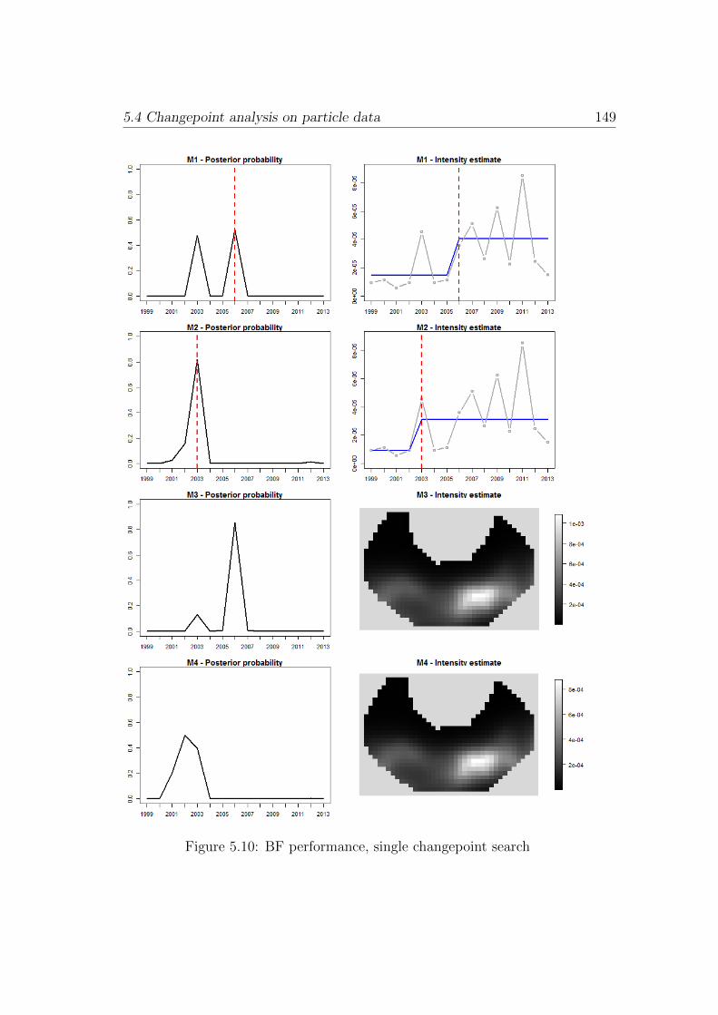
5.4 Changepoint analysis on particle data 149
Figure 5.10: BF performance, single changepoint search

150 5. Radioactive Particle Data Analysis
As happens when using the BF method with simulated data, there are
no changepoints detected in the two inhomogeneous models, despite the fact
that the spatial model posterior shows a very high peak, above 0.8, in 2006
and a second one in 2003, while the spatio-temporal model posterior has a
peak around 0.5 between 2002 and 2003. They are considered non-significant
using the BF method, therefore changepoints are present in the data series
only if fitting the two homogeneous models.
Posterior Threshold method
As for the PT method, threshold values are chosen based on the simula-
tion results: a low threshold of 0.2 for the first model, an only slightly greater
one, 0.25, for the second model, and much higher values, 0.85, for the third
and fourth model. In general, results are consistent with the simulation re-
sults: coherent conclusions with respect to the BF method results for the two
homogeneous models, but more changepoints detected when moving to the
inhomogeneous models. Results are all shown in Figure 5.11. Indeed, a sig-
nificant changepoint in 2006 is detected when fitting the fixed effect model,
with a peak raising high above the threshold; the second peak in 2003 is
also above the threshold, so, even if discarded at the moment because we
are looking for a single changepoint, it suggests the usefulness of a multiple
changepoint search. Coherent results with regard to the BF method are also
achieved with the second model: a major changepoint in 2003, determin-
ing an increase in the particle intensity. Results change with respect to the
BF method conclusions when fitting the spatial inhomogeneous model: the
peak in 2006 is considered significant, therefore the INLA estimates are split
into two images for the two segments, with a similar spatial structure and
a different scale. Here too, a visible second peak in 2003 hints at the need
to look for further changes. The posterior distribution of the fourth model,
showing a peak that reaches 0.5, does not raise above the threshold, therefore
no changepoints are detected when allowing for both spatial and temporal
dependence.

5.4 Changepoint analysis on particle data 151
Figure 5.11: PT performance, single changepoint search

152 5. Radioactive Particle Data Analysis
Results for the single changepoint search are summarised in Table 5.1.
Table 5.1: Single search - detected changepoints
Model Changepoint (BF) Changepoint (PT)
Fixed 2006 2006
Temporal 2003 2003
Spatial — 2006
Sp-temp — —
When looking at the data behaviour, models assuming a homogeneous in-
tensity do not seem very suitable for our data: the kernel intensity estimates
(Figure 5.5) show an inhomogeneous behaviour, whose structure is substan-
tially constant over time up to a scale parameter, with a main hot spot in
the bottom-right area and a second one in the bottom-left part, and lower
density in the top half of the window. This visual approach suggests data
are better described with the third or fourth model, and show a similar be-
haviour to the simulated data presented in Chapter 4, which kept a constant
spatial structure and only showed a change in scale. If further investigation
is of interest about the best model for the data, the Deviance Information
Criterion can be used as introduced in Section 3.5.
5.4.3 Multiple changepoint search results
Again, we follow the same procedure used for the simulation study, i.e. we
implement a binary segmentation algorithm combined with both BF and PT
methods, and then we try a simultaneous multiple changepoint search with
the recursive equation approach.
A summary of the resulting changepoints is given in Table 5.2.
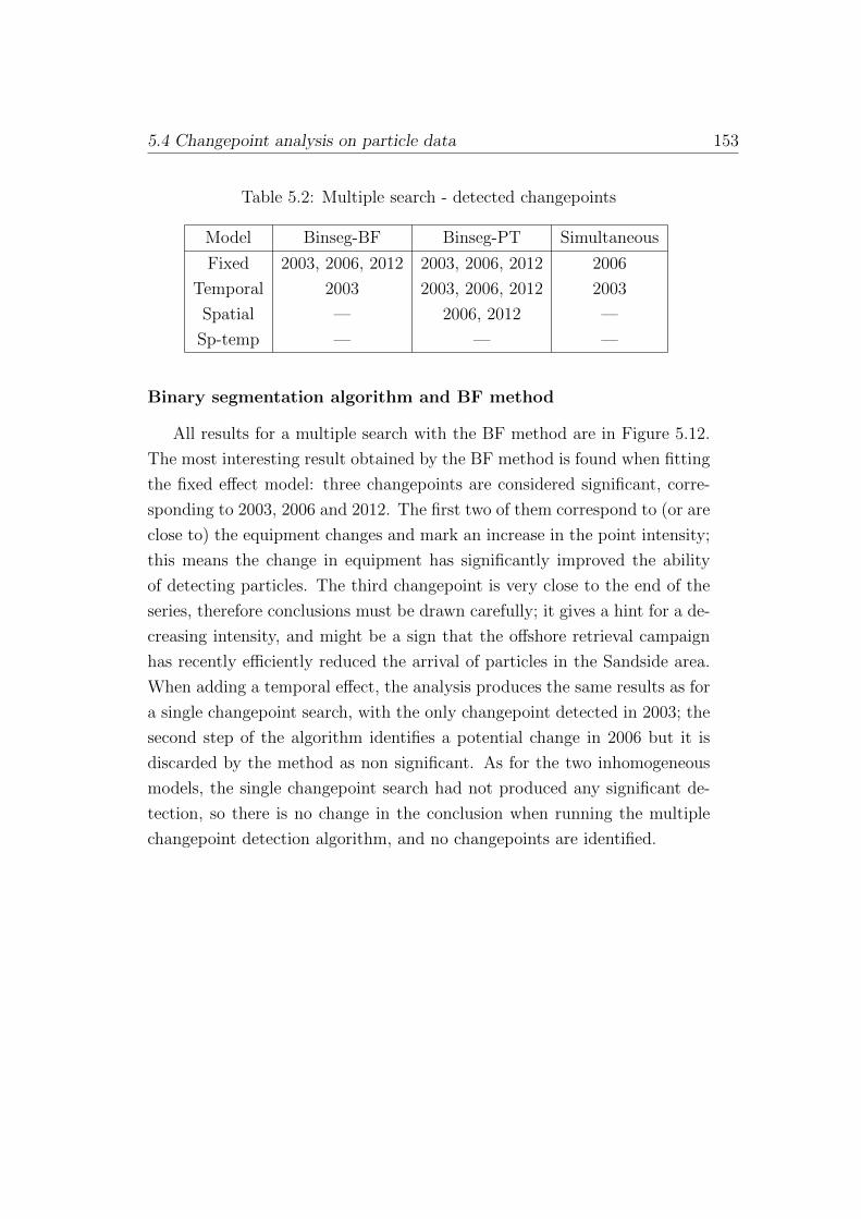
5.4 Changepoint analysis on particle data 153
Table 5.2: Multiple search - detected changepoints
Model Binseg-BF Binseg-PT Simultaneous
Fixed 2003, 2006, 2012 2003, 2006, 2012 2006
Temporal 2003 2003, 2006, 2012 2003
Spatial — 2006, 2012 —
Sp-temp — — —
Binary segmentation algorithm and BF method
All results for a multiple search with the BF method are in Figure 5.12.
The most interesting result obtained by the BF method is found when fitting
the fixed effect model: three changepoints are considered significant, corre-
sponding to 2003, 2006 and 2012. The first two of them correspond to (or are
close to) the equipment changes and mark an increase in the point intensity;
this means the change in equipment has significantly improved the ability
of detecting particles. The third changepoint is very close to the end of the
series, therefore conclusions must be drawn carefully; it gives a hint for a de-
creasing intensity, and might be a sign that the offshore retrieval campaign
has recently efficiently reduced the arrival of particles in the Sandside area.
When adding a temporal effect, the analysis produces the same results as for
a single changepoint search, with the only changepoint detected in 2003; the
second step of the algorithm identifies a potential change in 2006 but it is
discarded by the method as non significant. As for the two inhomogeneous
models, the single changepoint search had not produced any significant de-
tection, so there is no change in the conclusion when running the multiple
changepoint detection algorithm, and no changepoints are identified.

154 5. Radioactive Particle Data Analysis
Figure 5.12: BF performance, multiple changepoint search
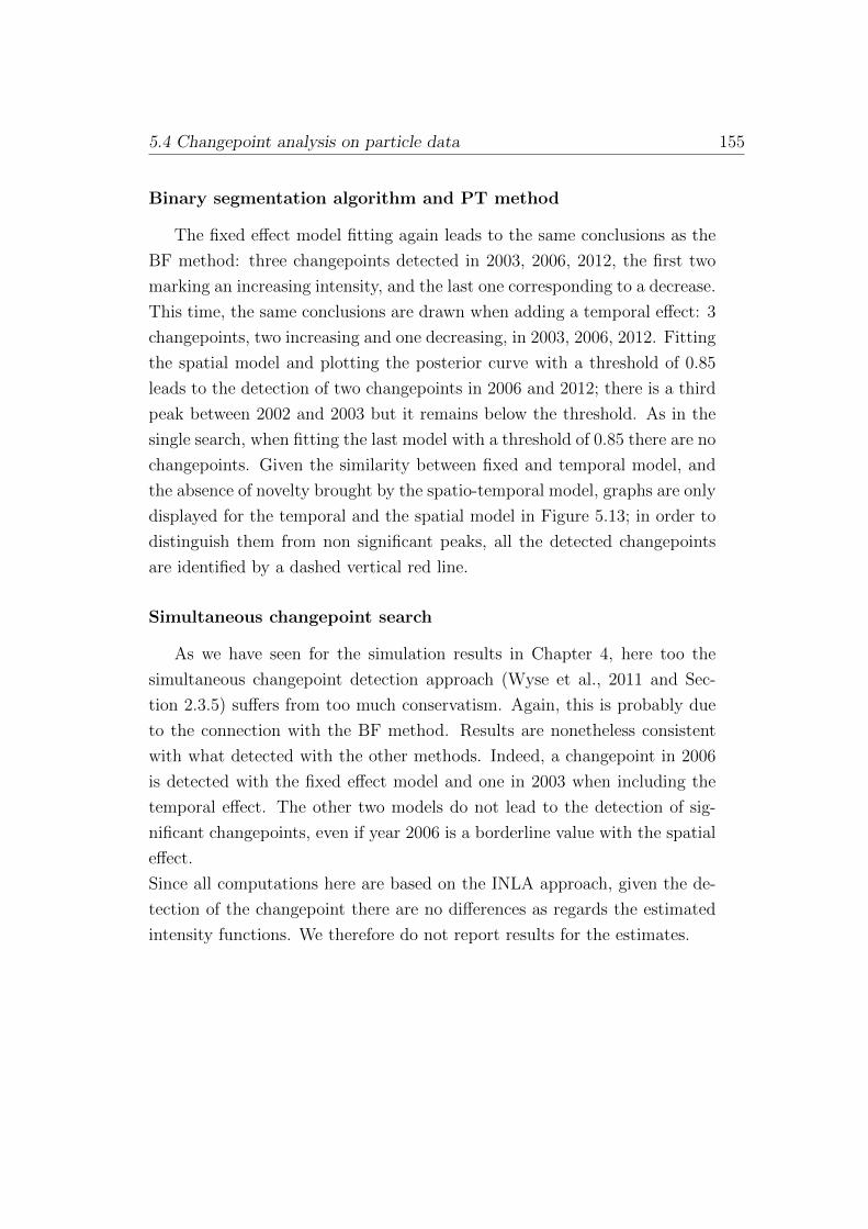
5.4 Changepoint analysis on particle data 155
Binary segmentation algorithm and PT method
The fixed effect model fitting again leads to the same conclusions as the
BF method: three changepoints detected in 2003, 2006, 2012, the first two
marking an increasing intensity, and the last one corresponding to a decrease.
This time, the same conclusions are drawn when adding a temporal effect: 3
changepoints, two increasing and one decreasing, in 2003, 2006, 2012. Fitting
the spatial model and plotting the posterior curve with a threshold of 0.85
leads to the detection of two changepoints in 2006 and 2012; there is a third
peak between 2002 and 2003 but it remains below the threshold. As in the
single search, when fitting the last model with a threshold of 0.85 there are no
changepoints. Given the similarity between fixed and temporal model, and
the absence of novelty brought by the spatio-temporal model, graphs are only
displayed for the temporal and the spatial model in Figure 5.13; in order to
distinguish them from non significant peaks, all the detected changepoints
are identified by a dashed vertical red line.
Simultaneous changepoint search
As we have seen for the simulation results in Chapter 4, here too the
simultaneous changepoint detection approach (Wyse et al., 2011 and Sec-
tion 2.3.5) suffers from too much conservatism. Again, this is probably due
to the connection with the BF method. Results are nonetheless consistent
with what detected with the other methods. Indeed, a changepoint in 2006
is detected with the fixed effect model and one in 2003 when including the
temporal effect. The other two models do not lead to the detection of sig-
nificant changepoints, even if year 2006 is a borderline value with the spatial
effect.
Since all computations here are based on the INLA approach, given the de-
tection of the changepoint there are no differences as regards the estimated
intensity functions. We therefore do not report results for the estimates.

156 5. Radioactive Particle Data Analysis
Figure 5.13: PT performance, multiple changepoint search

5.5 Inclusion of covariates 157
5.5 Inclusion of covariates
When introducing the dataset (Section 5.1), we listed the available infor-
mation including data on the radioactivity level and depth in the sediment of
the retrieved particles. This is part of the response and is usually referred to
in point process analysis as marks. Additional information is also available,
though, that is contextual and does not depend on the particles themselves;
it can be exploited to improve the models and further check the methods’
performance.
5.5.1 Introducing covariates
Two covariates in particular may be useful for analysing the particle dis-
tribution over Sandside beach: the distance from the nuclear discharge outlet,
that is considered the main source for particle dispersion, and the distance
from the ’low water level’, i.e. the northern boundary of the observation win-
dow, since the particle arrival from the offshore area must depend on tides
and currents.
Figure 5.14 shows both distances; as can be seen, the range of values is very
different as the low water level is part of the window border, while the nu-
clear discharge outlet is far away from the beach in the North-East direction.
We are inclined to believe that the nuclear discharge does not have a sig-
nificant effect on the distribution of particles, because the distance is high
and there are several intervening environmental processes; for instance, the
U-shaped coast around the beach (Figure 5.1) is likely to nullify potential
long-distance effects. Nevertheless, we test both covariates separately on our
data in order to check their ability to add useful information for describing
the phenomenon under study.

158 5. Radioactive Particle Data Analysis
Figure 5.14: Covariates (distance in metres)
5.5.2 Extensions of the models
We introduce the two covariates in our models, one at a time, as fixed
effects. The models become:
• Model 1: fixed effect and covariate
log λ(t) = µt + βtz + εt for t = 1, . . . , T
• Model 2: fixed effect, covariate and temporal effect
log λ(t) = µt + βtz + φt + εt for t = 1, . . . , T
• Model 3: intercept, covariate and spatial effect
log λ(t, s) = δ + βtz + ψts + εts for t = 1, . . . , T and s = 1, . . . , S
• Model 4: intercept, covariate, temporal effect and spatial effect
log λ(t, s) = δ + βtz + φt + ψts + εts for t = 1, . . . , T and s = 1, . . . , S.
We refer to Section 3.2.2 for details on the notation; here, z indicates the
single covariate. As usual, under H0 each effect takes a single value over
time, while under H1 it takes m + 1 values where m ≥ 1 is the unknown
number of changepoints. We apply all our detection methods considering
each covariate separately.
5.5.3 Results and discussion
A summary of the obtained results is in Tables 5.3 for a single changepoint
search and 5.5 for a multiple changepoint search.

5.5 Inclusion of covariates 159
Single search: comparison and comments
Table 5.3: Single search - detected changepoints with either covariate
Nuclear discharge Low water level
Model BF PT BF PT
Fixed 2003 2003 2006 2006
Temporal — 2003 — 2003
Spatial — 2006 — 2006
Sp-temp — — — —
When comparing Table 5.3 to Table 5.1, the first thing to note is that
with Model 1 (fixed) results depend on the covariate. Using the distance
from the low water level leads to the same results as the analysis without
covariates, while including the distance from the nuclear discharge outlet has
a similar effect to including a temporal component: year 2003 is chosen as
the changepoint. Besides, including a covariate in Model 2 (temporal) has a
negative effect on the BF method, since it is now unable to detect any change-
point. Results remain the same as regards Model 2 with the PT method and
Model 3 (spatial) and 4 (spatio-temporal) with either method and covariate.
In conclusion, when covariates are included in a single changepoint search
no increase in the ability to find changepoints takes place: the PT method
seems unaffected by covariates, and the BF method tends to be even more
conservative.
It would be of interest to carry out a model comparison and see if a model
with one of the covariates is preferred to the corresponding one with no co-
variate. The Deviance Information Criterion (DIC) may be used as it is
frequently used in Bayesian analysis for model selection. Since this is not
the main focus of our work, we only show an example of the DIC for a single
search and leave a deeper analysis for further studies; values are in Table 5.4.
In this Table, we can see that when using Model 1 the addition of the dis-
tance from the nuclear discharge improves the DIC, while the distance from
the low water level has no effect. As for Model 2, no improvements take
place: when using the BF method, no changepoints are found, so the DIC

160 5. Radioactive Particle Data Analysis
Table 5.4: Single search - DIC values
No covariate Nuclear discharge Low water level
Model BF PT BF PT BF PT
Fixed 599 599 234 234 598 598
Temporal 239 239 2080 243 2077 243
Spatial 1949 1864 1951 1081 1951 648
Sp-temp 1853 1853 1855 1855 1855 1855
under H0 is far higher than the other ones; when using the PT method, there
are no substantial changes. The DIC for Model 2 shows a consistent improve-
ment with respect to Model 1 when no covariate is used (the temporal model
would be chosen as the best model among the four of them), but the best
performance is given by the fixed model with the inclusion of the distance
from the nuclear discharge outlet. As regards Model 3, the inclusion of the
covariates has a strong positive effect, especially with the distance from the
low water level, if combined with the PT method: the model performs much
better than the one without covariates. No changepoints are detected with
Model 4 irrespective of the method and of the inclusion of covariates; H0 is
never rejected and all DICs are very high.
Multiple search: comparison and comments
The detected changepoint location for a binary segmentation procedure
with either the BF or the PT method and for a simultaneous approach are
reported in Table 5.5.
Table 5.5: Multiple search - detected changepoints with either covariate
Nuclear discharge Low water level
Model Binseg-BF Binseg-PT Simult Binseg-BF Binseg-PT Simult
Fixed 2003 2003 2006 2012 2003 2006 2003 2006 2012 2006
Temporal — 2003 2006 2012 — — 2003 2006 2012 —
Spatial — 2006 2012 — — 2006 2012 —
Sp-temp — — — — — —

5.6 Informative prior settings 161
The binary segmentation combined with the PT method is unaffected by
either covariate: results are exactly the same as in Table 5.2 for all models.
The binary segmentation with the BF method and the simultaneous search
lead to the same results, which are roughly the same as for the single search in
Table 5.3: in Model 1, the inclusion of the distance from the nuclear discharge
outlet shifts the changepoint from 2006 to 2003, while in Model 2 considering
any of the two covariates leads to the detection of no changepoint. No other
change occurs with respect to Table 5.2, and conclusions are extremely similar
to the simple single search ones.
Concluding remarks
This Section is only a first step towards the inclusion of covariates and
the search for a good model for the data. Different options for including
covariates can be tested: for instance, they can be modelled as smooth effects
or can be included jointly. In this work, we do not aim at a complete analysis
on the covariates; the scope of our work has already been clarified and focuses
on spatial and temporal dependence. Since the available information is of
interest on real data, though, we choose to give a hint of what can be done to
improve our models and to show that our methods still produce good results.
Indeed, linear dependence on a covariate does not substantially affect results
on these data. We are in general still able to detect changes and the only
relevant differences concern BF-based detection techniques: a changepoint is
detected in 2003 instead of 2006 when fitting Model 1 with the distance from
the nuclear discharge outlet, and no changepoint is detected in Model 2. A
comparison of the DIC values for the single search highlights a preference for
the first model combined with the distance from the nuclear discharge outlet,
or (with very close values) for the second model.
5.6 Informative prior settings
In the simulation study presented in Chapter 4, all prior distributions are
non informative, as the scope of the study is to test the ability of the meth-
ods to detect changepoints irrespective of the prior setting. When working

162 5. Radioactive Particle Data Analysis
with real data, though, prior knowledge can be of help in obtaining sensi-
ble results. In particular, one of the research questions presented in Section
1.1.2 concerns two known potential changepoints corresponding to equipment
changes. So far, we focused on the more general case of unknown locations,
but it is of interest to check the performance of our methods in the presence
of informative priors. Non vague prior distribution may, in this context, re-
gard the number of changepoints and/or their positions. We try both cases
separately.
5.6.1 Number of changepoints
Firstly, we focus on prior knowledge concerning the number of change-
points. Since we believe that there are two main changepoints, we focus on
multiple changepoint detection techniques, in particular on the simultaneous
search for two main reasons. First of all, the approach presented in Section
2.3.4 allows separate prior distributions on number and locations to be set;
secondly, the simultaneous approach produced conservative results on our
data (Section 5.4.3), so we are interested in improving the method by in-
cluding extra information. Moreover, the binary segmentation algorithms do
not need diffenrent prior distributions, as they have already detected the two
changepoints of interest in most cases with no addition of extra knowledge.
We compare results with four different prior settings: a non informative one
(presented in Section 5.4.3) and three different belief strengths:
1. Prior 1 - vague
π(m) = 0.25 for m = 0, 1, 2, 3
2. Prior 2 - weak
π(2) = 0.4
π(m) = 0.2 for m = 0, 1, 3
3. Prior 3 - medium
π(2) = 0.6
π(m) = 0.13 for m = 0, 1, 3
4. Prior 4 - strong

5.6 Informative prior settings 163
π(2) = 0.8
π(m) = 0.07 for m = 0, 1, 3
The four prior distributions are shown in Figure 5.15.
Figure 5.15: Prior settings on the number of changepoints
After choosing the priors, the same simultaneous changepoint search is
run; then, the conditional likelihoods L(Y |m), m = 0, . . . , 3 are multiplied by
the corresponding prior probability before choosing the highest one. Results
are displayed in Table 5.6. Note that the column referring to Prior 1 is the
same as the results displayed in Table 5.2, since the prior is non informative.
Table 5.6: Simultaneous search with different prior settings
Model Prior 1 Prior 2 Prior 3 Prior 4
Fixed 2006 2003,2006 2003,2006 2003,2006
Temporal 2003 2003,2006 2003,2006 2003,2006
Spatial — — 2003,2006 2003,2006
Sp-temp — — 2000,2003 2000,2003
With the first two models, a weak belief that there are two changepoints
is sufficient for detecting the changes in the equipment, while Model 3 and
4 allow for more data variability, therefore they need a strongly informative
prior setting in order to detect any change. When fitting Model 3, conclu-
sions are consistent with the rest of the results, while Model 4 leads to the
detection of a different changepoint in 2000, which had never been found
before. In conclusion, the use of an informative prior setting allows the first

164 5. Radioactive Particle Data Analysis
research question to be fully answered by detecting positive changes in the
intensity of the process corresponding, in most cases, to the improvements
in the equipment. The simultaneous approach is substantially improved by
the addition of extra knowledge via informative prior distributions, as its
conservatism is overcome.
5.6.2 Changepoint positions
Another option is to use information about the changepoint positions (in a
changepoint search with an unknown number of changepoints the two options
can be combined). Since the two equipment changes took place at the end
of 2002 and at the beginning of 2007, we fix peaks in the prior distributions
corresponding to 2003 and 2007, firstly one at a time (for a single search),
then jointly (for a multiple search). Three prior distributions with different
peak heights are set for each case, where the first one is non informative and
coincides with the previous analysis. For a single search with a prior peak in
2003
1. Prior 1 - vague
π(τ) = 0.083 for τ = 2000, . . . , 2011
π(τ) = 0 for τ = 1999, 2012, 2013
2. Prior 2 - weak
π(τ) = 0.2 for τ = 2003
π(τ) = 0.073 for τ = 2000, 2001, 2002, 2004, . . . , 2011
π(τ) = 0 for τ = 1999, 2012, 2013
3. Prior 3 - strong
π(τ) = 0.5 for τ = 2003
π(τ) = 0.045 for τ = 2000, 2001, 2002, 2004, . . . , 2011
π(τ) = 0 for τ = 1999, 2012, 2013
The same setting is replicated for a changepoint in 2007. Extreme values
have a null prior probability as we set a minimum segment length of 2 time
points.
For a multiple search

5.6 Informative prior settings 165
1. Prior 1 - vague
π(τ) = 0.083 for τ = 2000, . . . , 2011
π(τ) = 0 for τ = 1999, 2012, 2013
2. Prior 2 - weak
π(τ) = 0.2 for τ = 2003, 2007
π(τ) = 0.06 for τ = 2000, 2001, 2002, 2004, 2005, 2006, 2008, 2009, 2010, 2011
π(τ) = 0 for τ = 1999, 2012, 2013
3. Prior 3 - strong
π(τ) = 0.4 for τ = 2003, 2007
π(τ) = 0.02 for τ = 2000, 2001, 2002, 2004, 2005, 2006, 2008, 2009, 2010, 2011
π(τ) = 0 for τ = 1999, 2012, 2013
All prior distributions are displayed in Figure 5.16 (single peak) and 5.18
(multiple peaks).
Single changepoint detection
We fit Model 1 to 4 with six different prior settings, three for 2003 and
three for 2007, as shown in Figure 5.16. Then, we look for a changepoint
with both the BF and the PT method.
Figure 5.16: Prior settings on the changepoint position

166 5. Radioactive Particle Data Analysis
Results for the BF method are summarized in Table 5.7, while results for
the PT method are in Table 5.8.
In both Tables, it is immediate to see that the inclusion of an informative
Table 5.7: Single search with different prior settings and the BF method
Model Vague Prior on 2003 Prior on 2007
prior Prior 2 Prior 3 Prior 2 Prior 3
Fixed 2006 2006 2006 2006 2006
Temporal 2003 2003 2003 2003 2003
Spatial — — — — —
Sp-temp — — — — —
Table 5.8: Single search with different prior settings and the PT method
Model Vague Prior on 2003 Prior on 2007
prior Prior 2 Prior 3 Prior 2 Prior 3
Fixed 2006 2006 2006 2006 2006
Temporal 2003 2003 2003 2003 2003
Spatial 2006 — — 2006 —
Sp-temp — — 2003 — —
prior with a single peak does not affect the result in most cases. When
using the BF method, no difference in the results occurs. With the PT
method, changes in Model 3 results decrease the ability to find changes, as
the changepoint in 2006 is not detectable when imposing a prior peak on 2003
(or a very strong one on 2007); indeed, showing a preference for 2003 flattens
the other peaks so that 2006 becomes non significant, still the preference
is not powerful enough to raise the posterior probability in 2003 above the
threshold. The only new changepoint occurs when fitting Model 4 with a
strong prior on 2003: the posterior distribution raises above the threshold
thus, for the first time with respect to results deriving from non informative
priors, we have a significant changepoint with the spatio-temporal model.
We can see how posterior distributions change as we take different prior
distributions in Figure 5.17; the threshold for the PT method is also reported.

5.6 Informative prior settings 167
Figure 5.17: Posterior distributions resulting from different priors

168 5. Radioactive Particle Data Analysis
Multiple changepoint detection
We again fit Model 1 to 4 with different prior settings for two changepoints
corresponding to the equipment changes (Figure 5.18). We use both the
binary segmentation algorithm and the simultaneous approach to look for
changepoints.
Figure 5.18: Prior settings for two changepoints
Results for the binary segmentation method are in Tables 5.9 and 5.10,
while changepoints detected with the simultaneous approach are summarised
in Table 5.11.
Table 5.9: Multiple changepoint search with different prior settings, the bi-
nary segmentation algorithm and the BF method
Model Vague Prior on 2003 and 2007
prior Prior 2 Prior 3
Fixed 2003 2006 2012 2003 2006 2012 2003 2006 2012
Temporal 2003 2003 2003
Spatial — — —
Sp-temp — — —
As for the single search with the BF method, a multiple changepoint
analysis with the binary segmentation and the BF method (Table 5.9) does
not depend on the prior distributions on the changepoint locations: results
are identical to what obtained with a vague prior (see also Table 5.2). Again,
there is an analogy to the single search when using the PT method; fitting

5.7 Discussion 169
Table 5.10: Multiple changepoint search with different prior settings, the
binary segmentation algorithm and the PT method
Model Vague Prior on 2003 and 2007
prior Prior 2 Prior 3
Fixed 2003 2006 2012 2003 2006 2012 2003 2006 2012
Temporal 2003 2006 2012 2003 2006 2012 2003 2006 2012
Spatial 2006 2012 — —
Sp-temp — — 2003
Table 5.11: Simultaneous multiple changepoint search with different prior
settings
Model Vague Prior on 2003 and 2007
prior Prior 2 Prior 3
Fixed 2006 2003 2003
Temporal 2003 2003 2003
Spatial — — —
Sp-temp — — —
Model 3 with an informative prior on 2003 and 2007 decreases the ability to
detect changes, which become non significant. The improvement in Model 4
also occurs with a multiple search: when imposing strong peaks, the change-
point in 2003 raises above the threshold.
With a simultaneous approach, there is no improvement in the ability to de-
tect changepoints; it is to remark that a non vague prior leads to preferring
a changepoint in 2003 rather than in 2006 even with the fixed model.
5.7 Discussion
In this Chapter, we go back to the original research questions that mo-
tivated the whole study, after providing all the needed methodology and
method assessment: since the performance of the methods has already been
evaluated with simulated data, we know when to rely on the results and when

170 5. Radioactive Particle Data Analysis
they can be, e.g., too conservative.
We first follow the usual preliminary steps in a point process analysis. We test
Complete Spatial Randomness with MCMC distance based tests and reject
it in favour of a clustering behaviour. We motivate the use of Log-Gaussian
Cox processes via goodness of fit tests and privilege this class of models over
others for reasons such as flexibility and compatibility with INLA, which pro-
vides fast estimates even for complex models. After choosing the right class
of models, we can apply our new changepoint methods and draw conclusions
on the data behaviour. As a last step, we add some external information such
as including covariates and trying informative prior settings on the number
or locations of the changepoints.
According to the overall results, both the improvements in the equipment
and the offshore retrieval process have had positive effects in the intensity
of the process. The constance in the spatial structure of the intensity sug-
gests that future search of radioactive particles should emphasise the bottom
part of the Sandside beach, where the greater number of particles tends to
concentrate.
5.7.1 Remarks on standard changepoint analysis
Firstly, we carried out the same changepoint analysis as in Chapter 4,
with no addition/change in the models.
Results must be interpreted carefully since the time series is very short, but
they are sensible given the context, and there is a general, comforting con-
sistency over all the results: two major changes are detected, corresponding
to two peaks in the posterior probability of the changepoint position. They
correspond to 2003 and 2006, and they both mark an increase in the inten-
sity function. The spatial structure of the function remains approximately
the same, with higher values in the bottom half of the observation window
and lower values in the top half; its strength, or scale, increases after the
two changes. We know from the data history that two major changes in the
equipment used to detect the particles have taken place, one at the end of
2002 and the following at the beginning of 2007. We then hoped to find two
positive significant changes in 2003 and 2007; results are very close to what

5.7 Discussion 171
expected, with a shift of one year in the second change that might be due to
natural random oscillation in the data. When running a single changepoint
analysis, there are no different changepoints found. For both BF and PT
methods, we note that the peak in 2003 is favoured when including temporal
dependence in the model, while the change in 2006 is detected for the fixed
and spatial models. This supports the thesis of a positive random increase
in the data just before the second change: if we do not consider time depen-
dence in the data series, the peak in 2006 is detected first, probably because
it is the greatest in terms of scale shift. When including time dependence,
though, this peak becomes smaller than the one in 2003, thus the temporal
model results suggest that part of the change in 2006 is imputable to time
dependence. Despite this, the second peak is still visible in all models and
must not be discarded. Therefore, there is good support for stating that the
changes in the equipment have been effective in improving the ability to find
nuclear particles in the area.
As for the multiple changepoint search, the two peaks in 2003 and 2006 are
still among the detected ones, with, again, a preference for the first one in
the temporal model and for the second one in the fixed effect and spatial
model. In addition, a further change in 2012 is detected when a binary seg-
mentation algorithm is implemented. The third change point is very close
to the end of the series, therefore conclusions must be drawn with a special
care; it gives a hint of a decreasing intensity, which could be related to the
offshore retrieval campaign, suggesting a reduction of the arrival of particles
on Sandside beach.
5.7.2 Inclusion of extra information
In this Chapter, we also bring some novelty with regard to what has been
done so far, as we take a first step towards the inclusion of external knowl-
edge to potentially improve the models in order to explain the phenomenon
under study better.
First of all, we add two possible covariates, the distance to the nuclear dis-
charge outlet that is presumably responsible for the particle spreading off-
shore, and the distance from the low water level; we refit all the models and

172 5. Radioactive Particle Data Analysis
apply all our methods including one covariate at a time. In general, we can
say the distance from the low water level has a scarce effect on the change-
point detection, while the distance from the nuclear discharge outlet leads
to a preference for the changepoint in 2003. Apart from this effect, the PT
method (both in a single and multiple detection context) shows no changes
when either covariate is included. The effect on the BF based search and on
the simultaneous approach is negative as results become even more conser-
vative. A comparison of the DIC values (that depend on the number and
location of the detected changepoints) shows the preferred options are the
temporal model with no covariate or with the distance from the low water
level, or the fixed model with the distance from the nuclear discharge outlet.
Model 3 and 4 have higher DICs because of the inability to detect significant
changes.
Then, we exploit knowledge concerning the two changes in the equipment to
set informative prior distributions on the number or locations of the change-
points. As for their number, different peak heights on m = 2 are tested
with the simultaneous approach. This leads to a substantial increase in the
method performance, as regards the number of changes: the conservatism
is overcome, two changepoints are detected, results are consistent about the
changepoint locations and, above all, when imposing a stronger prior the
changes in the equipment become significant even with more complex mod-
els. For the first time, we detect changepoints with the spatio-temporal
model. Fixing an informative prior on the number of changepoints has a
more positive effect than a prior on the changepoint locations. When setting
peaks corresponding to 2003 and 2007, the only remarkable modification in
the results concerns the PT method: with a strong prior, a changepoint in
2003 is detected with Model 4. No other substantial changes or improve-
ments take place; in general, the changepoint in 2003 is preferred to the one
in 2006/2007. This is probably also due to the fact that the change in the
equipment that took place at the end of 2002 is more radical than the second
one (see Section 5.1).
Further steps in the analysis of the process should extend the inclusion of
available information to marks, such as the depth in the sediment or the
radioactivity level, and focus on finding the best model for the data.

Chapter 6
Conclusions and Final
Discussion
Detailed concluding remarks regarding specific aspects of our work can be
found at the end of each Chapter. In this final Chapter, we firstly summarise
the project and the main findings. Afterwards, we highlight the novelty and
contribution of our work to the fields of changepoint analysis and of point
process analysis and we motivate the choice of a Bayesian approach. Lastly,
a few hints at possible further directions for the study and the most recent
developments are outlined.
6.1 Work review
Our work aims at developing new methods for a changepoint analysis
on the inhomogeneous intensity function of a spatio-temporal point process.
We consider the most general case of multiple unknown changes, and are
interested in both detecting the change locations and estimating the change
type and its magnitude. Dealing with spatio-temporal data, the estimated
intensity for each time segment is a two dimensional pixel image. Estimates
of the segment parameters are not always the first goal of a changepoint anal-
ysis, as sometimes the interest only lies in detecting where the changepoint
lies, however our method also provides accurate estimates for a wide range
of problems.
173

174 6. Conclusions and Final Discussion
6.1.1 Assumptions
The assumptions and restrictions that need to be made when using our
methods are not strong. The process can be inhomogeneous and the intensity
function is only constrained to be smooth. Any type of change over time can
be detected: in scale, in spatial distribution or in both. Any prior setting
is acceptable and only influences the total computational time, which is still
feasible and can be further improved thanks to recent developments in the
INLA methodology, if needed. Data are Poisson distributed in our work but
may follow any distribution. There is no independence assumption except
between time segments. Dependence can be both spatial and temporal, either
small scale dependence or wide and smooth, either strong or weak, as long as
all the parameters can be assumed to belong to a Gaussian Field. There is no
limitation on the number of changepoints and reasonably weak assumptions
on their locations (they have to be ’not too close’ to each other). Therefore,
this method covers a very wide range of real situations.
6.1.2 Work summary
We start by presenting the motivating issues which include both theoret-
ical and practical questions.
As for the theory, we want to know what happens if a changepoint analysis
is run on a spatio-temporal point process instead of traditional time series:
first of all we have three dimensions, two spatial and one temporal, and
we want our method to be able to keep the information about all of them;
secondly, we can have different types of change over time and our method
should be able to detect any of them and, ideally, to distinguish between
them; besides, the dataset is quite complex and a long computational time
may be required to obtain results. The other theoretical assumption that
is usually made in changepoint analysis is that data are i.i.d.. If they are
not, spatio-temporal data can show many types of dependence, both in space
(between events at a specific time point) and in time (within time segments);
in particular, when temporal dependence is allowed, traditional changepoint
detection techniques do not offer a solution as, except for trivial situations,
the segment marginal likelihood is not tractable. This generates a need for

6.1 Work review 175
fast and accurate approximate computational methods.
As for the practical aspect, we have an interesting dataset concerning the
collection of radioactive particles on a beach, and the objective consists in
understanding the behaviour of the underlying process over time, with par-
ticular focus on two changes in the particle detection equipment that have
desirably marked an increased ability to find the particles, and on an offshore
retrieval campaign that should have recently reduced the arrival of particles
onshore.
As a second step in our work, we briefly present the three main topics our
study is built on: point processes, INLA and changepoint analysis. We give a
general introduction to all of them and present the most recent works in those
fields, then we focus on the aspects that are most useful for our project. As
for point processes, we introduce the class of spatio-temporal Log-Gaussian
Cox Processes, a broad and flexible class of models particularly suitable for
environmental applications. As for INLA, after a general introduction we
explain in detail how the fitting of a LGCP works and how it is possible to
overcome the intractability issue. As regards changepoint analysis, the most
recent challenge is of particular interest for us, concerning how to include
temporal dependence in time series data.
From Chapter 3 on, the contribution of our work is presented. We first give a
few options for setting the prior distributions on number and locations of the
changepoints; we introduce four increasingly complex LGCPs for both a sin-
gle and a multiple changepoint detection; then, after obtaining the posterior
distribution of the changepoint locations we propose some different methods
for taking decisions on which changepoints are significant and which are not.
Lastly, we present two methods, an iterative and a simultaneous one, to carry
out a multiple changepoint search.
A complex simulation study follows, where the performance of our models
and methods, the accuracy and the computational time of the INLA method-
ology are evaluated. We cover a wide range of real situations by generating
both i.i.d. and time dependent data, both from a homogeneous and an inho-
mogeneous process, with zero, one or multiple changes; we also try all types
of temporal change, in scale, in spatial structure and in both. In general, our
method proves to work; it suffers from too much conservatism when using

176 6. Conclusions and Final Discussion
some of the methods, still it is overall satisfactory; whenever changepoints
are detected, the methods are very accurate in estimating the changepoint
location(s) and producing good estimates for the process intensity at every
time segment.
As a last stage, all the proposed models and methods are applied to the moti-
vating dataset in order to answer the motivating practical questions. Firstly,
we reproduce the study carried out on simulated data, then we extend it by
adding covariates and introducing informative prior distributions on num-
ber and locations of the changes. In general, we find sensible results, as the
equipment changes correspond to a significant increase in the intensity func-
tion of the process, while a decrease toward the end of the series gives a hint
for effectiveness in reducing the quantity of particles that arrive onshore.
6.1.3 Meeting the research questions
We have positively answered all our research questions, both theoreti-
cal and practical. Our approach is effectively able to detect any type of
changepoint over time in the intensity of a spatio-temporal point process,
even when spatial heterogeneity, spatial dependence and temporal depen-
dence within segments are allowed. The computational time is satisfactory,
as results only take a few minutes for every dataset, and this is very useful
because it allows many different models to be fit and model comparison and
selection to be run in a feasible time despite the complexity of the data. Re-
sults are in general good (improvements in some of the methods are left to
further studies) and the application to real data leads to sensible interpreta-
tion of the phenomenon under study.
One of our motivating questions is to look for potential changepoints at
known locations (equipment changes). We firstly address the question using
the general technique for unknown locations for two main reasons. First of
all, the other practical question concerns unknown changes and needs to be
addressed this way; secondly, the case of known changepoints can easily be
derived as a special case of our method by imposing informative priors (see
Section 6.3 for a discussion), thus we prefer to propose a method that is able
to cover a wider range of issues. We also showed an example of what happens

6.2 Contribution of the work 177
in the special case of an informative prior on 2 changepoints and of a high
prior probability of having a changepoint corresponding to the equipment
changes. In general, results have not been affected by the priors as they
were already very good; it is worth mentioning that an informative prior
on the number of changepoints has substantially increased the ability of the
simultaneous approach to detect changes.
6.2 Contribution of the work
Spatial statistic and changepoint analysis are two well established ar-
eas of statistical research, but they do not meet often. A combination of
changepoint analysis and point processes is even rarer, and we have very
few examples of this in recent literature. These examples all deal with a
temporal process, and it usually is a simple Poisson process; nevertheless,
analyses are complex. The extension of changepoint analysis to spatial stud-
ies is uncommon, therefore it is even rarer to find works focused on looking
for changepoints in the parameters of a spatio-temporal model, irrespective
of the type of available data. In particular, as far as changepoints in spatio-
temporal point processes are concerned the subject is totally unexplored.
Nevertheless, questions and issues are raised, as is the case of our motivating
dataset, that need to be answered by developing new methods and extending
the existing ones.
A changepoint analysis on spatio-temporal point processes, therefore, would
be a novelty itself in statistical studies. It would extend the currently used
methods even if it were dealing with a very simple case, like a homogeneous
Poisson process with i.i.d. point patterns within segments. Our work aims
at doing more than providing an extension of simple models: it aims at de-
veloping methods able to cover a wide range of real situations.
The second novelty is the inclusion of dependence within time segments; as
we deal with spatio-temporal data, we include both spatial and temporal de-
pendence between data points. In the simulation study presented in Chapter
4, we show results for models allowing for temporal dependence between
point patterns, for spatial dependence between the points of a single point

178 6. Conclusions and Final Discussion
pattern, and for both.
The third novelty is the class of models we use, Log-Gaussian Cox Processes,
thanks to which we cover the case of inhomogeneous processes, and the pos-
sibility of spatial clustering and/or repulsion.
Moreover, we study changes in the scale of the intensity function (i.e. a
change in the expected number of points per pattern), in its spatial structure
(i.e. a change in the spatial distribution of points, with the same expected
number of events) and in both. This means our methods are able to cover
an extremely wide variety of real situation, and in particular many datasets
with a complex behaviour that are not easy to model and describe.
In addition to all this, our work provides a useful new case study of the INLA
performance. INLA is a young methodology and it is still unknown to a wide
part of the global statistical community. The number of case studies is in-
creasing but currently limited. In particular, there is a very small number of
published papers on point process models fitted with INLA and hardly any
work on changepoint analysis using INLA. Therefore, our work shows a new
way of exploiting the power and potential of the INLA approach.
As mentioned in Chapter 1, in the special case of a spatially homogeneous
spatio-temporal point process, the same results can be obtained in a simpler
way by running a changepoint analysis on the time series made by the num-
ber of points at every instant. This is hardly ever the case in real situations,
though, and our method is much more general as it not only considers how
many changepoints are present, but also where they occur. Therefore, if a
process is inhomogeneous or if we are not sure about what kind of process
we are facing, the use of our method avoids the risk of missing changes in the
spatial distribution of the points and brings more information by maintaining
the spatial dimension of the dataset.
Lastly, we add a few details that are often avoided in Bayesian inference:
despite our methods should theoretically work with any prior distribution,
we show it by running some sensitivity analysis on our real dataset and com-
paring posterior distributions deriving from different prior settings.
A further topic might be to face the issue of dependence across segments.
This is scarcely of interest in the situation of an abrupt change, where it is
sensible to assume independence after a changepoint occurs, but can open up

6.3 Discussion on the Bayesian approach 179
to other possibilities such as gradual changes. Still, our study is a consistent
step forward and a big challenge even without covering the case of depen-
dence across segments; moreover, as we use Log-Gaussian Cox Processes and
assume changes to be due to an external factor such as a change in the equip-
ment, the assumption of dependence within segments only fits the situation
well.
6.3 Discussion on the Bayesian approach
We build a Bayesian approach to face this complex changepoint issue. The
main reason is that we want to be able to incorporate external prior knowl-
edge in the model. In many real applications, experts of the phenomenon
under study have ideas of where, or approximately where, a changepoint
might be. Frequentist approaches, though, are very rigid, since only two
possibilities are considered. In an unknown changepoint search, all time
points have exactly the same probability of being a changepoint; in known
changepoint testing, only one (or a small number of) changepoint location(s)
is tested, and if there is an extra, unexpected changepoint it will be missed.
With a Bayesian approach, prior belief on the changepoint location(s) can
be included and the strength of this belief specified, as we do in our real data
application; in an extreme case, the prior mass may be concentrated on very
few points, but if knowledge is not that strong, a higher prior probability
can be assigned to a set of specific points, without excluding the other time
points from the analysis. This avoids the risk to miss significant unexpected
changes. A Bayesian setting substantially enriches the crude information
given by the data and allows for more flexibility.
Secondly, the issue of including dependence is recent and challenging, and
very few techniques are currently available; we have no knowledge of a fully
likelihood-based approach able to produce accurate results in such situations.
A Bayesian approach, combined with reliable approximate methods such as
INLA, returns posterior distributions and estimates for any kind of model
as long as the underlying assumptions hold. This way, we provide a method
that is able to give results that, in the worst case (i.e. total absence of prior

180 6. Conclusions and Final Discussion
knowledge) will equal the frequentist results that are currently unachievable
in this context; in any case where even weak prior knowledge is available,
likelihood-based conclusions will be improved by a Bayesian approach.
6.4 Hints for further studies
Our work combines recent literature from many different fields of statis-
tics, therefore it can be faced from different perspectives; this is very stimu-
lating, as each perspective gives suggestions for future directions and further
developments.
First of all, our work consists in a Bayesian approach. Doubtless, the most
important aspect of Bayesian statistics is the role of the prior distributions;
still, in most works this is hidden under the carpet. In our study, the main
goal that has been fulfilled is to be able to fit models with spatial and tem-
poral dependence, and a sensitivity analysis has been hinted at in Chapter
5. One of the next natural steps is therefore to carry out a complete work on
the priors that can concern the number of changepoints, their locations and
all the effects hyperparameters; it would certainly be of interest to test differ-
ent, more informative prior settings and check how strongly conclusions are
affected by them. As for the priors on number and positions of changepoints,
an alternative option is given in Fearnhead (2006) and Wyse et al. (2011); no
motivation is given for that specific setting, though, apart from its property
to reduce computation and increase the algorithm speed. Consequences on
the ability to detect changes should be further investigated. Another, more
informative setting can be given when there is knowledge about a possible
location for the change: one value, or a small set of adjacent values, can be
given a high a priori probability of being a changepoint.
A second filter for looking at our work is INLA. This approximate approach
is proving so effective in many situations that is now often used even for non
fully Bayesian analyses. People interested in cases studies where INLA is
employed will find an original contribution here, as there is very little done
in recent literature on point processes and even less on spatio-temporal ex-
tensions or changepoint detection. As for further work in this field, improve-
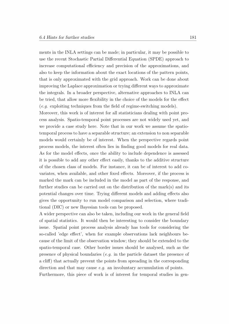
6.4 Hints for further studies 181
ments in the INLA settings can be made; in particular, it may be possible to
use the recent Stochastic Partial Differential Equation (SPDE) approach to
increase computational efficiency and precision of the approximations, and
also to keep the information about the exact locations of the pattern points,
that is only approximated with the grid approach. Work can be done about
improving the Laplace approximation or trying different ways to approximate
the integrals. In a broader perspective, alternative approaches to INLA can
be tried, that allow more flexibility in the choice of the models for the effect
(e.g. exploiting techniques from the field of regime-switching models).
Moreover, this work is of interest for all statisticians dealing with point pro-
cess analysis. Spatio-temporal point processes are not widely used yet, and
we provide a case study here. Note that in our work we assume the spatio-
temporal process to have a separable structure; an extension to non separable
models would certainly be of interest. When the perspective regards point
process models, the interest often lies in finding good models for real data.
As for the model effects, once the ability to include dependence is assessed
it is possible to add any other effect easily, thanks to the additive structure
of the chosen class of models. For instance, it can be of interest to add co-
variates, when available, and other fixed effects. Moreover, if the process is
marked the mark can be included in the model as part of the response, and
further studies can be carried out on the distribution of the mark(s) and its
potential changes over time. Trying different models and adding effects also
gives the opportunity to run model comparison and selection, where tradi-
tional (DIC) or new Bayesian tools can be proposed.
A wider perspective can also be taken, including our work in the general field
of spatial statistics. It would then be interesting to consider the boundary
issue. Spatial point process analysis already has tools for considering the
so-called ’edge effect’, when for example observations lack neighbours be-
cause of the limit of the observation window; they should be extended to the
spatio-temporal case. Other border issues should be analysed, such as the
presence of physical boundaries (e.g. in the particle dataset the presence of
a cliff) that actually prevent the points from spreading in the corresponding
direction and that may cause e.g. an involuntary accumulation of points.
Furthermore, this piece of work is of interest for temporal studies in gen-

182 6. Conclusions and Final Discussion
eral, and changepoint analysis in particular. This is a specific field in time
series analysis that does not often meet with other traditional approaches,
for instance what is called trend analysis. It would be interesting to further
extend the analysis to gradual changes in the intensity function, and compare
its performance with a study of the spatio-temporal trend of the series.
Lastly, as the work is motivated by practical questions on a real dataset, it is
possible to face this study from an applied perspective. This work can find
applications in many fields: ecology, forestry, epidemiology, crime, . . . . Since
the methodology has been well developed but the application only concerns
a short time series with few points, we suggest the production of another
case study with a larger spatio-temporal point process dataset.

Appendix A
Simulation - all figures
183

184 A. Simulation - all figures
Figure A.1: Single changepoint search on AR(1) data, with the fixed effect
model and the BF method

185
Figure A.2: Single changepoint search on iid data, with the temporal effect
model and the BF method

186 A. Simulation - all figures
Figure A.3: Single changepoint search on iid data, with the spatial effect
model and the BF method - Power level and location of the changepoint

187
Figure A.4: Single changepoint search on iid data, with the spatial effect
model and the BF method - Estimated intensities

188 A. Simulation - all figures
Figure A.5: Single changepoint search on AR(1) data, with the spatial effect
model and the BF method - Power level and location of the changepoint

189
Figure A.6: Single changepoint search on AR(1) data, with the spatial effect
model and the BF method - Estimated intensities

190 A. Simulation - all figures
Figure A.7: Single changepoint search on AR(1) data, with the spatio-
temporal effect model and the BF method - Power level and location of
the changepoint

191
Figure A.8: Single changepoint search on AR(1) data, with the spatio-
temporal effect model and the BF method - Estimated intensities

192 A. Simulation - all figures
Figure A.9: Single changepoint search on iid data, with the temporal effect
model and the PT method

193
Figure A.10: Single changepoint search on AR(1) data, with the temporal
effect model and the PT method
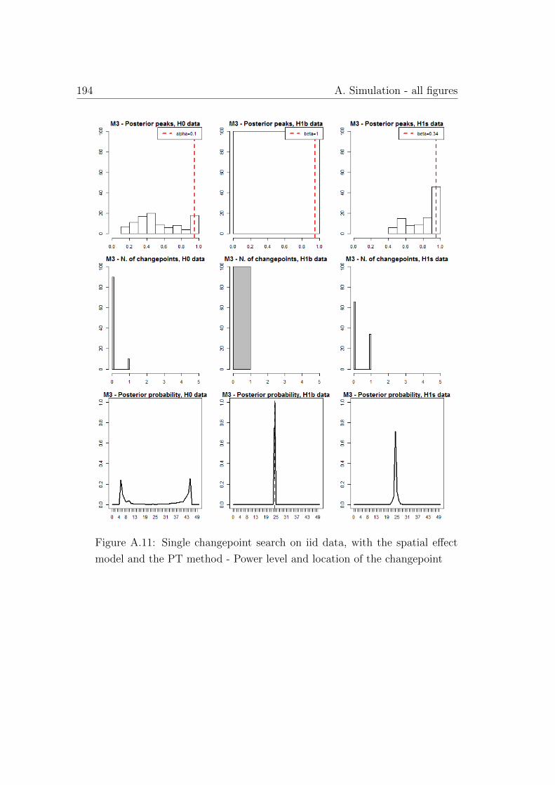
194 A. Simulation - all figures
Figure A.11: Single changepoint search on iid data, with the spatial effect
model and the PT method - Power level and location of the changepoint

195
Figure A.12: Single changepoint search on iid data, with the spatial effect
model and the PT method - Estimated intensities

196 A. Simulation - all figures
Figure A.13: Single changepoint search on iid data, with the spatio-temporal
effect model and the PT method - Power level and location of the changepoint

197
Figure A.14: Single changepoint search on iid data, with the spatio-temporal
effect model and the PT method - Estimated intensities

198 A. Simulation - all figures
Figure A.15: Single changepoint search on AR(1) data, with the spatio-
temporal effect model and the PT method - Power level and location of the
changepoint

199
Figure A.16: Single changepoint search on AR(1) data, with the spatio-
temporal effect model and the PT method - Estimated intensities

200 A. Simulation - all figures
Figure A.17: Multiple changepoint search on iid data, with the fixed effect
model and the BF method

201
Figure A.18: Multiple changepoint search on iid data, with the temporal
effect model and the BF method

202 A. Simulation - all figures
Figure A.19: Multiple changepoint search on iid data, with the spatial effect
model and the BF method - Power level and location of the changepoint

203
Figure A.20: Multiple changepoint search on iid data, with the spatial effect
model and the BF method - Estimated intensities

204 A. Simulation - all figures
Figure A.21: Multiple changepoint search on iid data, with the spatio-
temporal effect model and the BF method - Power level and location of
the changepoint

205
Figure A.22: Multiple changepoint search on iid data, with the spatio-
temporal effect model and the BF method - Estimated intensities

206 A. Simulation - all figures
Figure A.23: Multiple changepoint search on iid data, with the fixed effect
model and the PT method
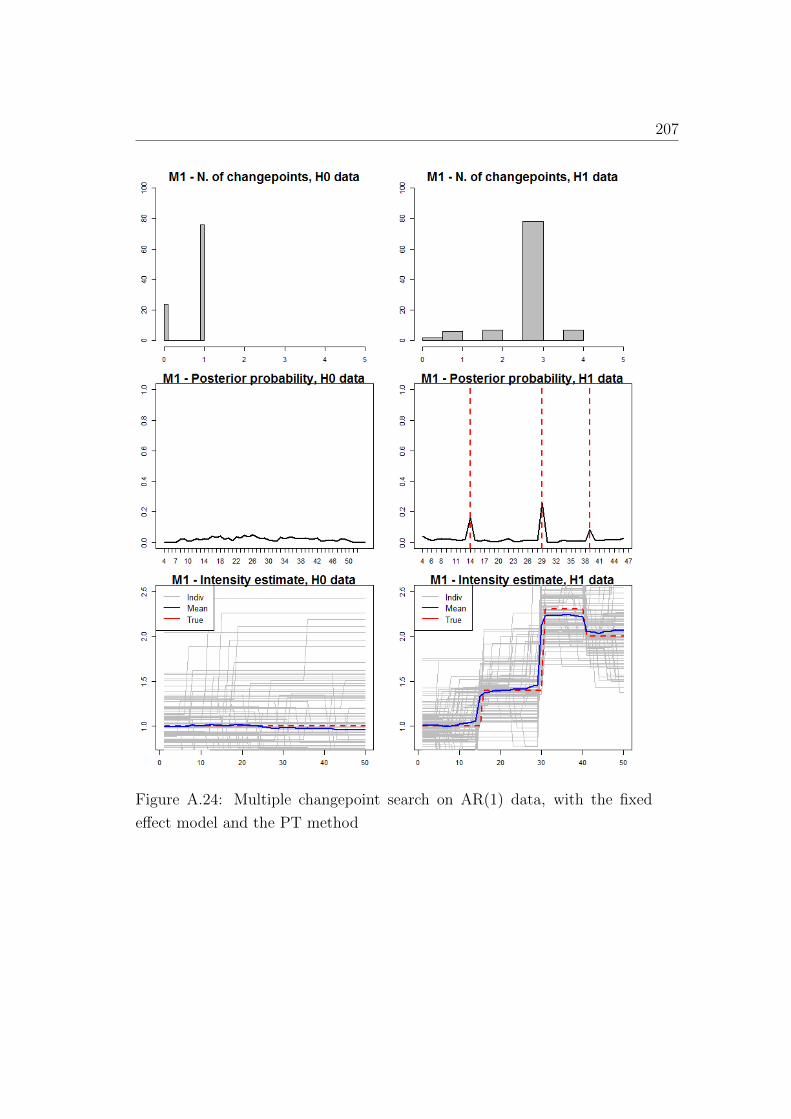
207
Figure A.24: Multiple changepoint search on AR(1) data, with the fixed
effect model and the PT method
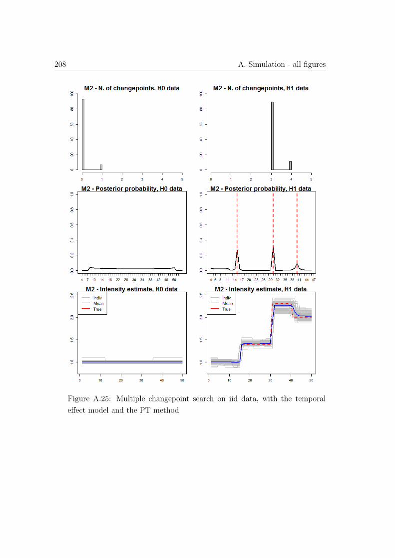
208 A. Simulation - all figures
Figure A.25: Multiple changepoint search on iid data, with the temporal
effect model and the PT method

209
Figure A.26: Multiple changepoint search on iid data, with the spatial effect
model and the PT method - Power level and location of the changepoint

210 A. Simulation - all figures
Figure A.27: Multiple changepoint search on iid data, with the spatial effect
model and the PT method - Estimated intensities

211
Figure A.28: Multiple changepoint search on iid data, with the spatio-
temporal effect model and the PT method - Power level and location of
the changepoint

212 A. Simulation - all figures
Figure A.29: Multiple changepoint search on iid data, with the spatio-
temporal effect model and the PT method - Estimated intensities

213
Figure A.30: Multiple changepoint search on AR(1) data, with the spatio-
temporal effect model and the PT method - Power level and location of the
changepoint

214 A. Simulation - all figures
Figure A.31: Multiple changepoint search on AR(1) data, with the spatio-
temporal effect model and the PT method - Estimated intensities

215
Figure A.32: Changepoint search on data with a change in the spatial struc-
ture, with the fixed effect model and the BF method

216 A. Simulation - all figures
Figure A.33: Changepoint search on data with a change in the spatial struc-
ture, with the temporal effect model and the BF method
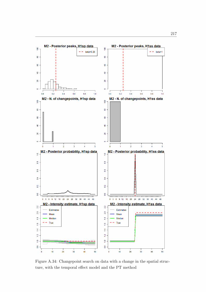
217
Figure A.34: Changepoint search on data with a change in the spatial struc-
ture, with the temporal effect model and the PT method

218 A. Simulation - all figures
Figure A.35: Changepoint search on data with a change in the spatial struc-
ture, with the spatial model and the BF method - Power level and location
of the changepoint

219
Figure A.36: Changepoint search on data with a change in the spatial struc-
ture, with the spatial model and the BF method - Estimated intensities

220 A. Simulation - all figures
Figure A.37: Changepoint search on data with a change in the spatial struc-
ture, with the spatial model and the PT method - Power level and location
of the changepoint

221
Figure A.38: Changepoint search on data with a change in the spatial struc-
ture, with the spatial model and the PT method - Estimated intensities
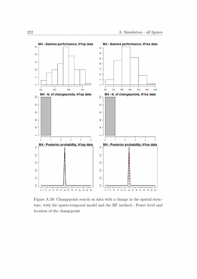
222 A. Simulation - all figures
Figure A.39: Changepoint search on data with a change in the spatial struc-
ture, with the spatio-temporal model and the BF method - Power level and
location of the changepoint

223
Figure A.40: Changepoint search on data with a change in the spatial struc-
ture, with the spatio-temporal model and the BF method - Estimated inten-
sities


Bibliography
Altieri, L., E. M. Scott, D. Cocchi, and J. B. Illian. A changepoint analysis
of spatio-temporal point processes. Submitted to Spatial Statistics .
Baddeley, A. and R. Turner (2005). spatstat: An R package for analyzing
spatial point patterns. Journal of Statistical Software 12, Issue 6.
Baddeley, A. and R. Turner (2006). Modelling spatial point patterns in R.
Case Studies in Spatial Point Process Modeling 185, 23–74.
Baddeley, A. J. (2010). Analysing spatial point patterns in R. Technical
report, CSIRO and University of Western Australia.
Baddeley, A. J., M. Berman, N. I. Fisher, A. Hardegen, R. K. Milne,
D. Schuhmacher, R. Shah, and R. Turner (2010). Spatial logistic regres-
sion and change-of-support in Poisson point processes. Electronic Journal
of Statistics 4, 1151–1201.
Baddeley, A. J., J. F. Coeurjolly, E. Rubak, and R. Waagepetersen (2013).
Logistic regression for spatial Gibbs point processes. Biometrika, 1–16.
Baddeley, A. J., J. Møller, and A. G. Pakes (2006). Properties of residuals
for spatial point processes. Technical report, Aalborg University.
Baddeley, A. J. and G. Nair (2012). Fast approximation of the intensity of
Gibbs point processes. Electronic Journal of Statistics 6, 1155–1169.
Baddeley, A. J., E. Rubak, and J. Møller (2011). Score, pseudo-score and
residual diagnostics for spatial point process models. Statistical Science 26,
613–646.
225

226 BIBLIOGRAPHY
Baddeley, A. J. and R. Turner (2000). Practical maximum pseudolikelihood
for spatial point patterns. Australian & New Zealand Journal of Statis-
tics 42, 283–322.
Baddeley, A. J., R. Turner, J. Møller, and M. Hazelton (2005). Residual
analysis for spatial point processes. Journal of the Royal Statistical Society
B 67, 617–666.
Baddeley, A. J. and M. N. M. Van Lieshout (1995). Area-interaction point
processes. Annals of the Institute of Statistical Mathematics 47, 601–619.
Barry, D. and J. A. Hartigan (1993). A Bayesian analysis for change point
problems. Journal of the American Statistical Association 88, 309–319.
Barthelme, S., H. Trukenbrod, R. Engbert, and F. Wichmann (2013). Mod-
elling fixation locations using spatial point processes. Journal of Vision 13.
Beaulieu, C., T. B. M. J. Ouarda, and O. Seidou (2010). A Bayesian normal
homogeneity test for the detection of artificial discontinuities in climatic
series. International Journal Of Climatology 30, 2342–2357.
Berman, M. and R. Turner (1992). Approximating point process likelihoods
with GLIM. Journal of the Royal Statistical Society C 41, 31–38.
Besag, J. (1975). Statistical analysis of non-lattice data. The Statistician 24,
179–195.
Blangiardo, M., M. Cameletti, G. Baio, and H. Rue (2013). Spatial and
spatio-temporal models with R-INLA. Spatial and Spatio-temporal Epi-
demiology 4, 33–49.
Blaszczyszyn, B. and D. Yogeshwaran (2013). Clustering comparison of point
processes with applications to random geometric models. In V. Schmidt
(Ed.), Stochastic Geometry, Spatial Statistics and Random Fields: Analy-
sis, Modeling and Simulation of Complex Structures.
Bondesson, L. and J. Fahlen (2003). Mean and variance of vacancy for hard-
core disc processes and applications. Scandinavian Journal of Statistics 30,
797–816.

BIBLIOGRAPHY 227
Brix, A. and P. Diggle (2001). Spatiotemporal prediction for log-Gaussian
Cox Processes. Journal of the Royal Statistical Society B 63, 823–841.
Brown, M. and G. J. Shanthikumar (1998). Comparing the variability of
random variables and point processes. Probability in the Engineering and
Informational Sciences 12, 425–444.
Cameletti, M., a. L. F., H. Rue, and D. Simpson (2013). Spatio-temporal
modelling of particulate matter concentration through theSPDE approach.
Advances in Statistical Analysis 97, 109–131.
Chatelain, F., A. Costard, and O. J. J. Michel (2011). A Bayesian marked
point process for object detection. Application to muse hyperspectral data.
In IEEE (Ed.), IEEE International Conference on Acoustics, Speech and
Signal Processing (ICASSP), pp. 3628–3631.
Chen, J. and A. K. Gupta (2012). Parametric Statistical Changepoint Anal-
ysis. Second Edition. Boston: Birkhauser.
Clyde, M. and D. Strauss (1991). Logistic regression for spatial pair-potential
models. Lecture Notes-Monograph Series 20, 14–20.
Cressie, N. and L. B. Collins (2001). Analysis of spatial point patterns
using bundles of product density LISA functions. Journal of agricultural,
biological and environmental statistics 6, 118–135.
Cressie, N. and C. K. Wikle (2011). Statistics for spatio-temporal data. Hobo-
ken: John Wiley & Sons.
Cseke, B., A. Z. Mangion, G. Sanguinetti, and T. Heskes (2013). Sparse
approximations in spatio-temporal point process models. arXiv:1305.4152
[stat.ML] .
Daley, D. J. (1981). Distances of random variables and point processes.
Technical report, Department of Statistics, University of North Carolina.
Daley, D. J. and D. Vere-Jones (2003). An Introduction to the Theory of
Point Processes. New York: Springer-Verlag.

228 BIBLIOGRAPHY
Dao, N. A. and M. G. Genton (2014). A Monte Carlo adjusted goodness-of-
fit test for parametric models describing spatial point patterns. Journal of
Computational and Graphical Statistics 23.
Dass, S. C., C. Y. Lim, and T. Maiti (2011). Hierarchical spatial regres-
sion models for change point analysis. In A. S. Association (Ed.), JSM
Proceedings, Survey Research Methods Section, pp. 3119–3133.
Dehling, H., A. Rooch, and M. S. Taqqu (2013). Power of change-point tests
for long-range dependent data. arXiv:1303.4917 [math.ST] .
Deng, Y. L. (1985). On the comparison of point processes. Journal of Applied
Probability 22, 300–313.
Diggle, P. (2006). Spatio-temporal point processes, partial likelihood, foot
and mouth disease. Statistical Methods in Medical Research 15, 325–336.
Diggle, P., P. Moraga, B. Rowlingson, and B. M. Taylor (2013). Spatial and
spatio-temporal log-Gaussian Cox Processes: extending the geostatistical
paradigm. Statistical Science 28, 542–563.
Diggle, P. J. (2000). Spatial statistics for environmental epidemiology. Tech-
nical report, Lancaster University.
Diggle, P. J. (2005). Spatio-temporal point processes: Methods and applica-
tions. Johns Hopkins University, Dept. of Biostatistics Working Papers 78.
Diggle, P. J. (2014). Statistical Analysis of Spatial and Spatio-Temporal Point
Patterns. Third Edition. Boca Raton: Taylor & Francis Group.
Diggle, P. J. and A. Brix (2001). Spatiotemporal prediction for log-Gaussian
Cox Processes. Journal of the Royal Statistical Society. Series B 63, 823–
841.
Diggle, P. J. and A. G. Chetwynd (1991). Second-order analysis of spatial
clustering for inhomogeneous populations. Biometrics 47, 1155–1163.
Dounreay-Particle-Advisory-Group (2006). Third report. Technical report,
Scottish Environment Protection Agency.

BIBLIOGRAPHY 229
Dounreay-Particle-Advisory-Group (2008). Fourth report. Technical report,
Scottish Environment Protection Agency.
Dounreay-Particle-Advisory-Group (2012). Dounreay Site Restoration Lim-
ited. Annual report. Technical report, Scottish Environment Protection
Agency.
Duan, J. A., A. E. Gelfand, and C. F. Sirmans (2010). Space-time point
process models using differential equations with application to urban de-
velopment.
Eckley, I. A., P. Fearnhead, and R. Killick (2011). Analysis of changepoint
models. In C.-A. T. Barber, D and C. U. P. Chiappa, S. (Eds.), Bayesian
Time Series Models, pp. Chapter 10.
Erdman, C. and J. W. Emerson (2007). bcp: An R package for perform-
ing a Bayesian analysis of change point problems. Journal of Statistical
Software 23, Issue 3.
Fahrmeir, K. (2006). Propriety of posteriors in structured additive regression
models: Theory and empirical evidence. Sonderforschungsbereich 386,
Paper 510.
Fearnhead, P. (2006). Exact and efficient Bayesian inference for multiple
changepoint problems. Statistics and Computing 16, 203–213.
Fearnhead, P. and L. Ziu (2011). Efficient Bayesian analysis of multiple
changepoint models with dependence across segments. Statistics and Com-
puting 21, 217–229.
Gatrell, A. C., T. C. Bailey, P. J. Diggle, and B. S. Rowlingson (1996). Spatial
point pattern analysis and its application in geographical epidemiology.
Transactions of the Institute of British Geographers 21, 256–274.
Gelfand, A. E., P. J. Diggle, M. Fuentes, and P. Guttorp (2010). Handbook
of Spatial Statistics. Boca Raton: Taylor & Francis Group.
Giraitis, L., G. Kapetanios, and T. Yates (2014). Inference on stochastic
time-varying coefficient models. Journal of Econometrics 179, 46–65.

230 BIBLIOGRAPHY
Gomez-Rubio, V., R. S. Bivand, and H. Rue (2014). Spatial models using
Laplace approximation methods. Handbook of Regional Science, 1401–
1417.
Gotway, C. A. and L. J. Young (2002). Combining incompatible spatial data.
Journal of the American Statistical Association 97, 632–648.
Gurarie, E., R. D. Andrews, and K. L. Laidre (2009). A novel method
for identifying behavioural changes in animal movement data. Ecology
Letters 12, 395–408.
Hall, P., B. U. Park, and B. A. Turlach (2002). Rolling-ball method for esti-
mating the boundary of the support of a point-process intensity. Annales
de l’Institut Henri Poincare 38, 959–971.
Hanks, E. M., M. B. Hooten, D. S. Johnson, and J. T. Sterling (2011).
Velocity-based movement modeling for individual and population level in-
ference. Technical report, PLoS ONE 6(8):e22795.
Held, L., B. Schrodle, and H. Rue (2010). Posterior and cross-validatory
predictive checks: A comparison of MCMC and INLA. Statistical Modelling
and Regression Structures , 91–110.
Illian, J. (2006). Combining geostatistical and point process modelling. In
Proceedings of METMA3.
Illian, J., A. Penttinen, H. Stoyan, and D. Stoyan (2008). Statistical Analysis
and Modelling of Spatial Point Patterns. Chichester: Wiley.
Illian, J. B. (2012). A toolbox for fitting complex spatial point process models
using integrated nested Laplace approximation (INLA). The Annals of
Applied Statistics 6, 1499–1530.
Illian, J. B. and D. K. Hendrichsen (2010). Gibbs point process models with
mixed effects. Environmetrics 21, 341–353.
Illian, J. B., S. Martino, S. H. Sørbye, J. B. Gallego-Fernandez, M. Zun-
zunegui, M. P. Esquivias, and J. M. J. Travis (2013). Fitting complex

BIBLIOGRAPHY 231
ecological point process models with integrated nested Laplace approxi-
mation. Methods in Ecology and Evolution 4, 305–315.
Illian, J. B., H. S. Sørbye, H. Rue, and D. K. Hendrichsen (2012). Using INLA
to fit a complex point process model with temporally varying effects. A case
study. Journal of Environmental Statistics 3.
Ivanoff, B. G. and E. Merzbach (2010). Optimal detection of a change-set in
a spatial Poisson process. The Annals of Applied Probability 20, 640–659.
James, B., K. L. James, and D. Siegmund (1987). Tests for a change-point.
Biometrika 74, 71–83.
Jandhyala, V., S. Fotopoulos, I. MacNeill, and P. Liu (2013). Inference for
single and multiple change-points in time series. Journal of time series
analysis .
Kallenberg, O. (1984). An informal guide to the theory of conditioning in
point processes. International statistical review 52, 151–164.
Killick, R. and I. A. Eckley (2011). changepoint: An R pack-
age for changepoint analysis. Technical report, Available online at
http://www.lancs.ac.uk/killick/Pub/KillickEckley2011.pdf.
Killick, R., P. Fearnhead, and I. A. Eckley (2012). Optimal detection of
changepoints with a linear computational cost. Journal of the American
Statistical Association 107, 1590–1598.
King, R., J. B. Illian, S. E. King, G. F. Nightingale, and D. K. Hendrichsen
(2012). A Bayesian approach to fitting Gibbs processes with temporal
random effects. Journal of Agricultural, Biological, and Environmental
Statistics 17, 601–622.
Krainski, E. T. and F. Lindgren (2013). The R-INLA tutorial: SPDE models.
Technical report, Available online at www.r-inla.org.
Liang, S., S. Banerjee, and B. P. Carlin (2009). Bayesian wombling for spatial
point processes. Biometrics 65, 1243–1253.

232 BIBLIOGRAPHY
Liang, S., B. P. Carlin, and A. E. Gelfand (2009). Analysis of Minnesota colon
and rectum cancer point patterns with spatial and nonspatial covariate
information. The annals of applied statistics 3, 943–962.
Lindgren, F. (2012). Continuous domain spatial models in R-INLA. The
ISBA Bulletin 19, No 4.
Lindgren, F. and H. Rue (2013). Bayesian spatial and spatio-temporal mod-
elling with R-INLA. Journal of Statistical Software.
Lindgren, F., H. Rue, and J. Lindstrom (2011). An explicit link between
Gaussian fields and Gaussian Markov random fields: the stochastic partial
differential equation approach. Journal of the Royal Statistical Society
B 73, Part 4, 423–498.
Liu, S., M. Yamada, N. Collier, and M. Sugiyama (2013). Change-point
detection in time-series data by relative density-ratio estimation. Neural
Networks 43, 72–83.
Mangion, A. Z., M. Dewar, V. Kadirkamanathan, and G. Sanguinetti (2012).
Point process modelling of the Afghan War Diary. Proceedings of the
National Academy of Sciences of the United States of America 109, 12414–
12419.
Mangion, A. Z., G. Sanguinetti, and V. Kadirkamanathan (2012). Variational
estimation in spatiotemporal systems from continuous and point-process
observations. IEEE Transactions on Signal Processing 60, 3449–3459.
Mangion, A. Z., K. Yuan, V. Kadirkamanathan, M. Niranjan, and G. San-
guinetti (2011). Online variational inference for state-space models with
point-process observations. Neural Computation 23, 1967–1999.
Martins, T. G., D. Simpson, F. Lindgren, and H. Rue (2013). Bayesian
computing with INLA: new features. Computational Statistics & Data
Analysis 67, 68–83.

BIBLIOGRAPHY 233
Matteson, D. S. and N. A. James (2014). A nonparametric approach for mul-
tiple change point analysis of multivariate data. Journal of the American
Statistical Association 109, 334–345.
Mehta, C. R., P. N. R. and P. Senchaudhuri (2000). Efficient Monte Carlo
methods for conditional logistic regression. Journal of the American Sta-
tistical Association 95, 99–108.
Møller, J., A. R. Syversveen, and R. P. Waagepetersen (1998). Log Gaussian
Cox Processes. Scandinavian Journal of Statistics 25, 451–482.
Møller, J. and R. P. Waagepetersen (2004). Statistical Inference and Simu-
lation for Spatial Point Processes. Boca Raton: Chapman and Hall/CRC.
Møller, J. and R. P. Waagepetersen (2007). Modern statistics for spatial
point processes. Scandinavian Journal of Statistics 34, 643–684.
Murphy, S. A. and P. K. Sen (1991). Time-dependent coefficients in a Cox-
type regression model. Stochastic Processes and their Applications 39,
153–180.
Park, T., R. T. Krafty, and A. I. Sanchez (2012). Bayesian semi-parametric
analysis of Poisson change-point regression models: application to policy
making in Cali, Colombia. Journal of Applied Statistics 39(10), 2285–2298.
R Development Core Team (2008). R: A Language and Environment for
Statistical Computing. Vienna, Austria: R Foundation for Statistical Com-
puting. ISBN 3-900051-07-0.
Raftery, A. E. (1993). Change point and change curve modeling in stochastic
processes and spatial statistics. Technical report, University of Washing-
ton.
Reeves, J., J. Chen, L. Wang, R. Lund, and Q. Lu (2006). A review and
comparison of changepoint detection techniques for climate data. Journal
of Applied Meteorology and Climatology 46, 900–915.
Ripley, B. D. (1977). Modelling spatial patterns. Journal of the Royal Sta-
tistical Society. Series B 39, 172–212.

234 BIBLIOGRAPHY
Ross, G. J. (2013). Parametric and nonparametric sequential change detec-
tion in R: The cpm package. Journal of Statistical Software.
Rue, H. and L. Held (2005). Gaussian Markov Random Fields. Theory and
Applications. Boca Raton: Chapman & Hall.
Rue, H., S. Martino, and N. Chopin (2009). Approximate Bayesian inference
for latent Gaussian models by using integrated nested Laplace approxima-
tions. Journal of the Royal Statistical Society B 71, Part 2, 319–392.
Shao, C., U. Mueller, and J. Cross (2011). Area-to-point Poisson kriging
analysis for lung cancer incidence in Perth areas. In ECU Publications
PRE. 2011.
Shao, X. and X. Zhang (2010). Testing for change points in time series.
Journal of the American Statistical Association 105, 1228–1240.
Simpson, D., J. B. Illian, F. Lindgren, H. S. Sørbye, and H. Rue (2012).
Going off grid: Computationally efficient inference for log-Gaussian Cox
Processes. Technical report, NTNU Technical report 10.
Simpson, D., F. Lindgren, and H. Rue (2011). Fast approximate infer-
ence with INLA: the past, the present and the future. Technical report,
arXiv:1105.2982v1 [stat.CO].
Sørbye, S. H. (2013). Tutorial: Scaling IGMRF-models in R-INLA. Technical
report, www.r-inla.org.
Stasinopoulos, D. M. and R. A. Rigby (2007). Generalized additive mod-
els for location scale and shape (GAMLSS) in R. Journal of Statistical
Software 23, Issue 7.
Sun, J. and S. N. Rai (2001). Non-parametric tests for the comparison of
point processes based on incomplete data. Scandinavian Journal of Statis-
tics 28, 725–732.
Sundardas, S. D. R. (2001). First- and second-order properties of spatiotem-
poral point processes in the space-time and frequency domains. PhD thesis.
BIBLIOGRAPHY 235
Taylor, B. M., T. M. Davies, B. S. Rowlingson, and P. J. Diggle (2013). lgcp:
Inference with spatial and spatio-temporal log-Gaussian Cox Processes in
R. Journal of Statistical Software 52, Issue 4.
Taylor, B. M. and P. J. Diggle (2014). INLA or MCMC? a tutorial and com-
parative evaluation for spatial prediction in log-Gaussian Cox Processes.
Journal of Statistical Computation and Simulation 84, 2266–2284.
Tyler, A. N., E. M. Scott, P. Dale, A. T. Elliott, B. T. Wilkins, K. Boddy,
J. Toole, and P. Cartwright (2010). Reconstructing the abundance of
Dounreay hot particles on an adjacent public beach in Northern Scotland.
Science of the Total Environment 408, 4495–4503.
Veen, A. and F. P. Schoenberg (2011). Goodness-of-fit assessment of point
process models based on K-function variants. Technical report, Depart-
ment of Statistics, UCLA, UC Los Angeles.
Waagepetersen, R. (2008). Estimating functions for inhomogeneous spatial
point processes with incomplete covariate data. Biometrika 95, 351–363.
Warton, D. I. and L. Shepherd (2010). Poisson point process models solve
the ’pseudo-absence problem’ for presence-only data in ecology. Annals of
Applied Statistics 4, 1383–1402.
Wyse, J., N. Friel, and H. Rue (2011). Approximate simulation-free Bayesian
inference for multiple changepoint models with dependence within seg-
ments. Bayesian Analysis 6, 501–528.
Yang, T. Y. and L. Kuo (2001a). Bayesian binary segmentation procedure for
a Poisson process with multiple changepoints. Journal of Computational
and Graphical Statistics 10, 772–785.
Yang, T. Y. and L. Kuo (2001b). Bayesian binary segmentation procedure for
a Poisson process with multiple changepoints. Journal of Computational
and Graphical Statistics 10, 772–785.
Zou, C., Y. Liu, P. Qin, and Z. Wang (2007). Empirical likelihood ratio test
for the change-point problem. Statistics & Probability Letters 77, 374–382.

236 BIBLIOGRAPHY
Zou, C., G. Yin, L. Feng, and Z. Wang (2014). Nonparametric maximum
likelihood approach to multiple change-point problems. Annals of Statis-
tics 42, 970–1002.


![[6740 - 16810]unidade1](https://img.dokumen.tips/doc/110x75/5571fc41497959916996da1f/6740-16810unidade1.jpg)