Genetic Epidemiology 22:41–51 (2002)

© 2002 Wiley-Liss, Inc.

A Bayesian Approach to the Transmission/Disequilibrium Test for Binary Traits

Varghese George 1* and Purushottam W. Laud 2

1Department of Biostatistics, University of Alabama, Birmingham2Division of Biostatistics, Medical College of Wisconsin, Milwaukee

The transmission/disequilibrium test (TDT) for binary traits is a powerful methodfor detecting linkage between a marker locus and a trait locus in the presence ofallelic association. The TDT uses information on the parent-to-offspring transmis-sion status of the associated allele at the marker locus to assess linkage or asso-ciation in the presence of the other, using one affected offspring from each set ofparents. For testing for linkage in the presence of association, more than one off-spring per family can be used. However, without incorporating the correlationstructure among offspring, it is not possible to correctly assess the association inthe presence of linkage. In this presentation, we propose a Bayesian TDT methodas a complementary alternative to the classical approach. In the hypothesis testingsetup, given two competing hypotheses, the Bayes factor can be used to weighthe evidence in favor of one of them, thus allowing us to decide between the twohypotheses using established criteria. We compare the proposed Bayesian TDTwith a competing frequentist-testing method with respect to power and type Ierror validity. If we know the mode of inheritance of the disease, then the jointand marginal posterior distributions for the recombination fraction (θ) and dis-equilibrium coefficient (δ) can be obtained via standard MCMC methods, whichlead naturally to Bayesian credible intervals for both parameters. Genet. Epidemiol.22:41–51, 2002. © 2002 Wiley-Liss, Inc.

Key words: association; Bayes factor; credible interval; likelihood; linkage; Markov chain MonteCarlo method

Contract grant sponsor: NIH; contract grant HL65203 (V.G.).

*Correspondence to: Varghese George, Ph.D., Department of Biostatistics, University of Alabama atBirmingham, 327N Ryals Public Health Building, 1665 University Boulevard, Birmingham, AL 35294-0022. E-mail: VGeorge@ms.soph.uab.edu

Received for publication 12 February 2001; Revision accepted 20 April 2001

42 George and Laud

INTRODUCTION

In the presence of population association (disequilibrium) between a marker anda disease, the allele sharing method or LOD score method may fail to detect linkageeven with very large sample size. The transmission-disequilibrium test (TDT) pro-posed by Spielman et al. [1993] is a novel and intuitively appealing alternative thattests for linkage or association between a marker locus and associated dichotomoustrait in the presence of the other. It compares the frequency of marker alleles transmit-ted to affected children with the frequency of marker alleles not transmitted, using theMcNemar chi-square test. The basic idea is that a heterozygous parent will transmit theassociated marker allele to the affected offspring more frequently than the alternatemarker allele. This test is valid regardless of the allele frequencies of the marker anddisease locus, penetrance, ascertainment procedure, and mode of inheritance. The onlyassumptions required for the test are that the contributions from the two parents areindependent and that there is no segregation distortion at the marker locus. Thus, forthe purpose of testing linkage, Spielman’s TDT has the advantage of not requiring dataon multiple affected family members or on unaffected sibs, although transmission tounaffected sibs should be studied if there is any doubt about segregation distortion, ormeiotic drive, at the marker locus. It is a valid and powerful test for linkage in thepresence of population association and for association in the presence of linkage (withsingle affected offspring). Thus, it serves as an alternative to more powerful methodssuch as the one proposed by Terwilliger and Ott [1992] for homogeneous populations.Also, the test is not affected by the ascertainment procedure, and it is robust againstpopulation stratification. Various extensions have been proposed for quantitative traits,multiple affected offspring, multiple alleles at the marker locus, extended pedigrees,etc. [Allison, 1997; Martin et al., 1997; Horvath and Laird, 1998; Spielman and Ewens,1998; George et al., 1999; Abecasis et al., 2000].

In this paper we propose a Bayesian alternative to Spielman’s TDT for binarytraits. We use both affected and unaffected offspring who are informative for link-age. Non-informative prior distributions are selected for the joint probabilities, p11 =P(an individual has the associated allele transmitted and has the disease) and p10 =P(an individual does not have the associated allele transmitted but has the disease).From the prior distributions and the likelihood function, we compute the Bayes fac-tor for the hypothesis of linkage. The Bayes factor is a meaningful measure of evi-dence conditional on the given data. We show through simulation studies that thisapproach leads to a test with good frequentist properties: high power and correctcontrol of the type I error.

Just as in case of the classical TDT, the Bayesian TDT does not require knowl-edge of the mode of inheritance of the disease. However, if it is known, then thejoint and marginal posterior distributions for the recombination fraction (θ) and dis-equilibrium coefficient (δ) can be obtained via standard Markov chain Monte Carlo(MCMC) methods. These lead naturally to Bayesian interval estimates for θ and δ.

A BAYESIAN TDT FOR H 1: LINKAGE VERSUS H 2: NO LINKAGE

Assume that the marker locus is diallelic with associated allele M. (If there aremore than two alleles, they can be treated as “M” and “not M”). As in Spielman’s

Bayesian TDT for Binary Traits 43

TDT, we use only offspring who are informative for linkage. These include, withrespect to the marker locus, all offspring of homozygous by heterozygous matingand homozygous offspring of heterozygous by heterozygous mating. Let Yi be thebinary disease status and Xi be the binary transmission status (in both cases, 1 = yesand 0 = no) of the ith offspring in the sample. Let Xi = –1 if the offspring isnoninformative. Letting p = P(M), under the assumption of random mating of theparents, define

k = P(Xi = 0) = P(Xi = 1) = p(1 – p)(2 – 3p + 3p2). (1)

Thus, the probability that an offspring is informative is 2k. So,

P(Xi = 0 | Xi ≠ –1) = P(Xi = 1 | Xi ≠ –1) = ½.

Let D denote the disease allele at the disease locus with q = P(D). The disequilib-rium parameter is then defined as, for example,

δ = P(DM) – pq = qP(M | D) – pq = q(λ – p). (2)

As Thomson and Bodmer [1979] showed, 0 < δ ≤ min{p(1 – q), (1 – p)q}, andtherefore it follows that p < λ ≤ min(p/q, 1).

Now, the joint probabilities of the disease status and the transmission status are

p11 = P(Yi = 1, Xi = 1 | Xi ≠ –1), p10 = P(Yi = 1, Xi = 0 | Xi ≠ –1),p01 = P(Yi = 0, Xi = 1 | Xi ≠ –1) = ½ – p11, andp00 = P(Yi = 0, Xi = 0 | Xi ≠ – 1) = ½ – p10. (3)

The sample data can be summarized into:

n11 = number of offspring with Yi = 1 and Xi = 1,n10 = number of offspring with Yi = 1 and Xi = 0,n01 = number of offspring with Yi = 0 and Xi = 1, andn00 = number of offspring with Yi = 0 and Xi = 0,

where n11 + n10 + n01 + n00 = n. So, the likelihood function with a random sample of ninformative offspring is given by the multinomial distribution as

Λ = − − < <01 10 001111 11 10 10 11 10(½ ) (½ ) , where 0 , ½.n n nnp p p p p p

We make the implicit assumption here that within a sibship, given the transmissionstatus, the disease status of siblings is independent. If this is not reasonable, it ispossible to incorporate some correlation structure for the disease status among mem-bers within sibships.

For a given pair of hypotheses (H1, H2), the Bayes factor in favor of H1 is theratio of the post-data odds of H1 to its pre-data odds, and it can be computed as theratio of the marginal densities of the data under the two hypotheses. The Bayes fac-

44 George and Laud

tor can be used to weigh evidence in favor of a hypothesis, taking into account theprior information and the information from the likelihood function. The use of Bayesfactors to compare scientific theories was first proposed by Jeffreys [1961]. Over thepast decade, its use has seen a dramatic increase, primarily due to computational ad-vances. Kass and Raftery [1995] provide an excellent overview of the literature on thistopic. In our case, the two hypotheses of interest are H1: θ < 0.5 (linkage) and H2: θ =0.5 (no linkage). Under H2, the probability of transmission of the associated markerallele is the same regardless of the affection status. Thus, the two hypotheses are equiva-lent to H1: p11 ≠ p10 and H2: p11 = p10. Let the common probability under H2 be denotedby p1 and its prior distribution by f(p1). Also, denote the joint prior distribution of (p11,p10) by f(p11, p10). Then the Bayes factor for H1 is given by BF = L1/L2, where

= − −∫ 10 01 0011

11 10

1 11 10 11 10 11 10 11 10

,

(½ ) (½ ) ( , ) , and,n n nn

p p

L p p p p f p p dp dp(4)

+ += −∫ 11 10 01 00

1

2 1 1 1 1(½ ) ( ) .n n n n

p

L p p f p dp (5)

The integrals in the Bayes factor are expectations with respect to prior distributions.If we choose a beta distribution (rescaled to the interval from 0 to 0.5) with param-eters α and β as the prior for all three parameters p11, p10, and p1, then under theassumption that p11 and p10 are independent, the numerator and the denominator ofthe Bayes factor simplify to

2

11 01 10 001

11 01 10 00

11 10 01 002

( ) ( ) ( ) ( )1 ( ), and

2 ( ) ( ) ( ) ( )

( ) ( )1 ( ).

2 ( ) ( ) ( )

n

n

n n n nL

n n n n

n n n nL

n

Γ + α Γ + β Γ + α Γ + βΓ α + β = × × Γ α Γ β Γ + + α + β Γ + + α + β

Γ + + α Γ + + βΓ α + β = × × Γ α Γ β Γ + α + β

Setting α = β = 1 yields uniform priors for p11, p10, and p1, and further simplifies theBayes factor.

To aid in the interpretation of the Bayes factor, Jeffreys [1961] proposed thefollowing rule of thumb: “when 1 < BF ≤ 3, there is evidence for H1, but it is notworth more than a bare mention; when 3 < BF ≤ 10, the evidence is positive; when10 < BF ≤ 100, the evidence is strong; when BF > 100 the evidence is decisive.” Aspointed out by Kass and Raftery [1995], these categories are not a precise calibrationof the Bayes factor but rather a descriptive statement about standards of evidence inscientific investigations.

Simulation Study of the Properties of the Procedure

To evaluate frequentist properties of the proposed method via power and type Ierror validity, we simulated 2,000 replicate sets of samples, each consisting of 200

Bayesian TDT for Binary Traits 45

nuclear families, each of two parents and four offspring, under the assumptions ofrandom mating of parents and no crossover interference. The disease allele (D) of arecessive trait locus was simulated with allele frequency q = 0.4. The associatedmarker (M) allele was simulated with allele frequency p = 0.5. From equation (1),the probability of informative offspring is 62.5%. Thus, the expected number of in-formative offspring per sample is 500, and we observed an average of 500.6. Link-age disequilibrium coefficient δ of 0.1 was achieved by choosing P(MD) = 0.3, P(md)= 0.4, P(Md) = 0.2, and P(mD) = 0.1. The simulation was repeated for six differentmodels listed in Table I, under different values of θ, penetrance and phenocopies.Empirical probabilities for the different categories of the Bayes factor based onJeffreys’ rule of thumb were computed and are also given in Table I. For example, totest the hypotheses of linkage (H1) versus no linkage (H2) under the model withcomplete penetrance and no phenocopies, a Bayes factor cut-off value of 10 gives anempirical type I error of 0.001 (the null hypothesis being H2) with power 99% and98% for recombination fractions 0.0 and 0.05, respectively. Under the model with75% penetrance and 5% phenocopies, the empirical type I error is still 0.001 withpower 92.0% and 85%.

To compare power, we also performed Spielman’s TDT on the 2,000 replicatesamples. We computed empirical critical values for the Bayes factor correspondingto various values of the significance levels α under the hypothesis of no linkage.These critical values were used to decide whether to reject the hypothesis of nolinkage for different values of θ. The percentage of the time the hypothesis is re-jected corresponds to the empirical power of the test. We also computed the empiri-cal power of Spielman’s TDT. The results for different values of α and θ, penetranceand phenocopies are given in Table II. Under complete penetrance and no pheno-copies, the power is very high for both methods, even though the Bayesian methodis consistently more powerful. In the more realistic genetic model with incompletepenetrance and phenocopies, the Bayesian approach is substantially more powerful.For example, with 75% penetrance and 5% phenocopies at α = 0.001, the power ofthe Bayesian approach is 85% compared with 62% for the frequentist method.

A BAYESIAN TDT WHEN MODE OF INHERITANCE IS KNOWN

If one knows the mode of inheritance of the disease, that information can beincorporated in computing the likelihood function, the Bayes factor, and the posteri-

TABLE I. Empirical Probabilities of Jeffreys’ Rule Based on Bayes Factor in Favor of LinkageFrom a Simulation of 2,000 Replicates (d = 0.1)

Model Bayes factor in favor of linkage

no. Model ≤ 1 ≤ 3 > 3 > 10 > 100

i θ = 0.0, penetrance = 1.0, phenocopy = 0.0 0.002 0.003 0.997 0.993 0.968ii θ = 0.05, penetrance = 1.0, phenocopy = 0.0 0.004 0.010 0.990 0.980 0.930iii θ = 0.5, penetrance = 1.0, phenocopy = 0.0 0.968 0.993 0.007 0.001 0.000

iv θ = 0.0, penetrance = 0.75, phenocopy = 0.05 0.018 0.035 0.965 0.920 0.796v θ = 0.05, penetrance = 0.75, phenocopy = 0.05 0.028 0.078 0.923 0.846 0.670vi θ = 0.5, penetrance = 0.75, phenocopy = 0.05 0.973 0.994 0.006 0.001 0.000

θ, recombination fraction between the trait and the marker loci; δ, disequilibrium coefficient.

46 George and Laud

ors. One would expect that the added information should result in more powerfultests to detect linkage in the presence of association. Also, we can calculate the jointand marginal posterior distributions of θ and δ, yielding full inference proceduresfor these parameters.

To illustrate this, consider the case in which the disease trait is known to berecessive with complete penetrance. It can be shown that the joint probabilities inequation (3) simplify to

= − + δ − θδ + δ + − − − δ − θδ= − − δ + θδ − − − δ + + + δ + θδ= − = −

11

10

01 11 00 10

{(1 )( ) )}{2 ( ) (1 )(2 ) }/ 2 ,

{( [(1 ) ] )}{2(1 )[(1 ) ] ( ) }/ 2 ,

½ and ½ ,

p p pq p pq p q pq k

p p p q p p q p q pq k

p p p p

(6)

where k is as defined in equation (1). For all parameters in the model, we use priordistributions that represent very little pre-data information. Thus, for p, q, and λ, wetake uniform distributions on their respective ranges. The prior for δ is induced bythe priors of p, q, and λ. The prior for the recombination fraction is taken as beta (½,½) rescaled to the interval from 0 to ½. This is motivated by two considerations.First, it is the non-informative transformation-invariant choice (often termed Jeffreys’prior) for a probability in a Bernoulli likelihood. More important, its shape (see Fig.1B) equally emphasizes values of θ near 0 (extreme tight linkage) and 0.5 (no link-age), these being of most concern in practice.

Now, given the transmission status (Xi) of the associated marker allele, the dis-ease status (Yi) of the i th offspring follows a Bernoulli distribution with parameter

−η = = = ≠ − = 111 10( 1 | , 1) 2 ,i ix x

i i i i iP Y X x X p p

where p11 and p10 are as given in equation (6). The joint likelihood of the randomsample is then

( ) −

=

Λ = η − η∏ 112

1

(1 ) ,i i

nn y y

i ii

TABLE II. Simulation-Based Comparison of Power Between the Bayesian and the FrequentistTDT (2,000 Replicates, d = 0.1)

Power

Penetrance = 1.0, phenocopy = 0.0 Penetrance = 0.75, phenocopy = 0.05

θ = 0.0 θ = 0.05 θ = 0.0 θ = 0.05

α Bayes Freq. Bayes Freq. Bayes Freq. Bayes Freq.

0.001 0.993 0.952 0.984 0.902 0.932 0.750 0.849 0.6230.005 0.996 0.981 0.990 0.962 0.964 0.875 0.920 0.7750.010 0.998 0.990 0.994 0.978 0.975 0.905 0.946 0.8400.020 0.999 0.994 0.996 0.987 0.995 0.939 0.965 0.8920.050 1.000 0.998 0.999 0.994 0.998 0.973 0.980 0.947

θ, recombination fraction between the trait and the marker loci; α, significant level; δ, disequilibriumcoefficient; Freq., frequentist.

Bayesian TDT for Binary Traits 47

where hi is a function of θ, δ, p, and q. This Bayesian model is graphically repre-sented in Fig. 2.

Under this model, the numerator of the Bayes factor corresponding to the hy-pothesis H1: θ < 0.5, given in equation (4), becomes

θ δ

= − − θ δ θ δ∫ 10 01 00111 11 10 11 10

, , ,

(½ ) (½ ) ( , , , ) ,n n nn

p q

L p p p p f p q d d dpdq

Fig. 1. Prior (broken line) and posterior (solid line) densities for delta (disequilibrium coefficient),theta (recombination fraction), p (marker allele frequency) and q (disease allele frequency) in A, B, C,and D, respectively. The prior for delta is induced from the uniform priors of p and q and their relation-ship to delta. The prior for theta is beta (½, ½) rescaled to the interval from 0 to ½. The likelihood isbased on one replicate sample from the simulated data.

48 George and Laud

where f(θ, δ, p, q) is the joint prior distribution of these parameters. As before, underH2: θ = 0.5, p11 = p10 = p1, where, in this case, p1 is a function of δ, p, and q.Therefore, the denominator of the Bayes factor, given in equation (5), becomes

+ +

δ

= − δ δ∫11 10

10 002 1 1

, ,

(½ ) ( , , ) ,n n

n n

p q

L p p f p q d dpdq

where f(δ, p, q) is the joint prior distribution of δ, p, and q. The integrals above canbe computed by numerical integration or by simulation approximations. As before,the Bayes factor can be used as a “test statistic” to decide between the two hypoth-eses. The simulation results are very similar to those in the previous section and notshown here. The marginal posterior distributions of θ and δ are obtained from theprior distributions and the likelihood function via standard MCMC methods.

To illustrate parameter estimation, we randomly picked one replicate samplefrom the simulated data under the hypothesis of linkage, and analyzed it using thesoftware package BUGS [Spiegelhalter et al., 1995], which uses MCMC techniques[Brooks, 1998; Carlin and Louis, 2000]. These methods generate random samplesfrom the posterior distribution by running a Markov chain whose steady-state distri-bution equals the desired posterior distribution. The model depicted in Fig. 2 alongwith the precise relationships (described in the Methods section) among the variousnodes is conveyed to BUGS by a simple program (available on request). The gener-ated samples must then be subjected to convergence diagnostics to ensure that theMarkov chain has attained its steady state. In our case, we discarded the first 2,000iterations of the chain and then retained every eighth iteration of the next 8,000. This

Fig. 2. Graphic representation of the Bayesianmodel. Nodes represent various parameter and dataelements and arrows show interdependenciesamong them. Here, q = disease allele (D) fre-quency; p = associated marker allele (M) fre-quency; l = P(D|M); δ = disequilibrium coefficient;θ = recombination fraction between the trait andthe marker loci; Xi = 1 if M is transmitted, 0 if nottransmitted, –1 if non-informative; Yi = 1 if dis-ease is present, 0 otherwise; p11 = P(Yi = 1, Xi = 1 |Xi ≠ –1); p10 = P(Yi = 1, Xi = 0 | Xi ≠ –1); ηi =P (Yi = 1 | Xi = xi,Xi ≠ –1) = 2pxi

11p101–xi.

Bayesian TDT for Binary Traits 49

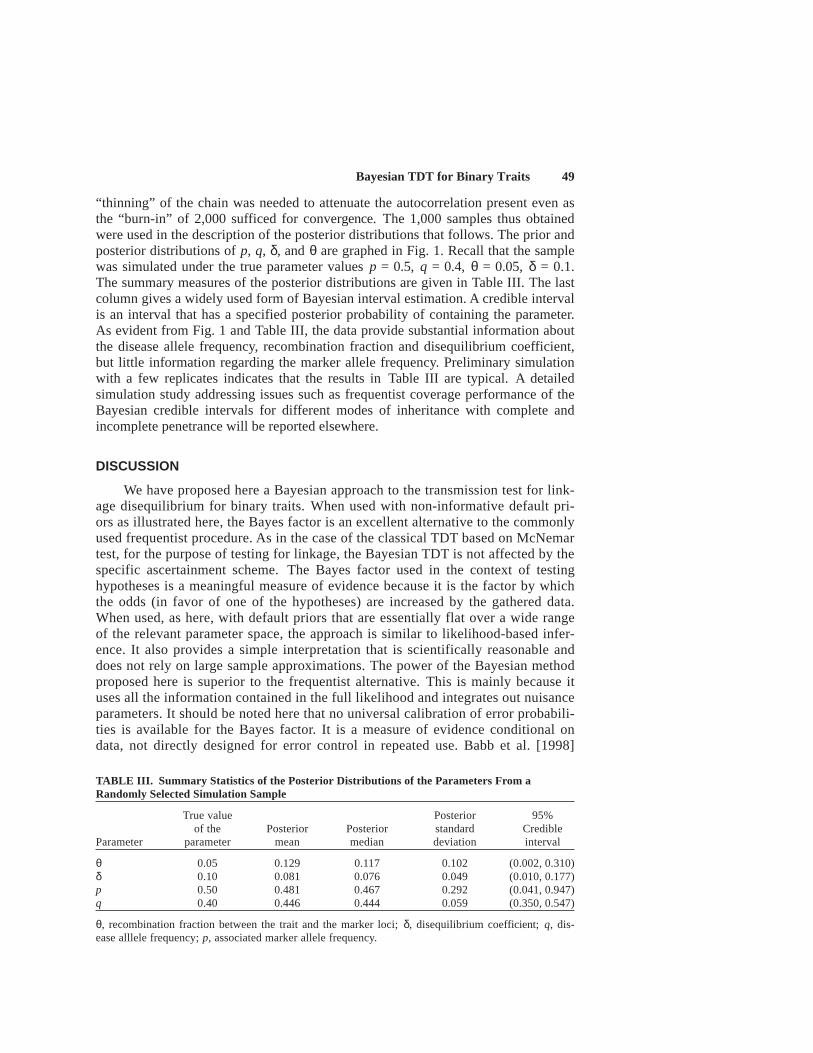
“thinning” of the chain was needed to attenuate the autocorrelation present even asthe “burn-in” of 2,000 sufficed for convergence. The 1,000 samples thus obtainedwere used in the description of the posterior distributions that follows. The prior andposterior distributions of p, q, δ, and θ are graphed in Fig. 1. Recall that the samplewas simulated under the true parameter values p = 0.5, q = 0.4, θ = 0.05, δ = 0.1.The summary measures of the posterior distributions are given in Table III. The lastcolumn gives a widely used form of Bayesian interval estimation. A credible intervalis an interval that has a specified posterior probability of containing the parameter.As evident from Fig. 1 and Table III, the data provide substantial information aboutthe disease allele frequency, recombination fraction and disequilibrium coefficient,but little information regarding the marker allele frequency. Preliminary simulationwith a few replicates indicates that the results in Table III are typical. A detailedsimulation study addressing issues such as frequentist coverage performance of theBayesian credible intervals for different modes of inheritance with complete andincomplete penetrance will be reported elsewhere.

DISCUSSION

We have proposed here a Bayesian approach to the transmission test for link-age disequilibrium for binary traits. When used with non-informative default pri-ors as illustrated here, the Bayes factor is an excellent alternative to the commonlyused frequentist procedure. As in the case of the classical TDT based on McNemartest, for the purpose of testing for linkage, the Bayesian TDT is not affected by thespecific ascertainment scheme. The Bayes factor used in the context of testinghypotheses is a meaningful measure of evidence because it is the factor by whichthe odds (in favor of one of the hypotheses) are increased by the gathered data.When used, as here, with default priors that are essentially flat over a wide rangeof the relevant parameter space, the approach is similar to likelihood-based infer-ence. It also provides a simple interpretation that is scientifically reasonable anddoes not rely on large sample approximations. The power of the Bayesian methodproposed here is superior to the frequentist alternative. This is mainly because ituses all the information contained in the full likelihood and integrates out nuisanceparameters. It should be noted here that no universal calibration of error probabili-ties is available for the Bayes factor. It is a measure of evidence conditional ondata, not directly designed for error control in repeated use. Babb et al. [1998]

TABLE III. Summary Statistics of the Posterior Distributions of the Parameters From aRandomly Selected Simulation Sample

True value Posterior 95%of the Posterior Posterior standard Credible

Parameter parameter mean median deviation interval

θ 0.05 0.129 0.117 0.102 (0.002, 0.310)δ 0.10 0.081 0.076 0.049 (0.010, 0.177)p 0.50 0.481 0.467 0.292 (0.041, 0.947)q 0.40 0.446 0.444 0.059 (0.350, 0.547)

θ, recombination fraction between the trait and the marker loci; δ, disequilibrium coefficient; q, dis-ease alllele frequency; p, associated marker allele frequency.

50 George and Laud

show, however, that it is possible to give theoretical bounds on error probabilitiesfor some Bayesian decision rules.

The incorporation of the mode of inheritance allows us to obtain estimates ofthe recombination fraction and the disequilibrium coefficient through Bayesian cred-ible intervals as illustrated in the case of recessive traits. Similar analyses can becarried out for dominant or codominant disease traits. Expressions similar to equa-tion (6) need to be derived in each case. While inferences obtained are accurate forall finite sample sizes, their validity depends on correct choice of the mode of inher-itance. Robustness with respect to incorrect specification of the model needs carefulinvestigation.

All these inferences have the potential to be even more powerful if meaningfulinformative priors can be constructed using knowledge from the literature or histori-cal data. While the feasibility of such priors has been demonstrated in other contexts[Kadane, 1980; Ibrahim et al., 1998], special attention should be given to possiblepopulation heterogeneity and to avoiding publication bias.

Finally, it is worth noting that the Bayesian approach used here for binary traitcan be extended to quantitative traits and to more complex models involving familialcorrelation, complex pedigree structure, etc. Clearly, the particulars of the computa-tional methods are different in each case.

ACKNOWLEDGMENT

This work was supported in part by NIH grant HL65203 (V.G.).

REFERENCES

Abecasis GR, Cardon LR, Cookson WOC. 2000. A general test of association for quantitative traits innuclear families. Am J Hum Genet 66:279–92.

Allison DB. 1997. Transmission-disequilibrium tests for quantitative traits. Am J Hum Genet 60:676–90.Brooks SP. 1998. Markov chain Monte Carlo method and its application. Statistician 47:69–100.Babb J, Rogatko A, Zacks S. 1998. Bayesian sequential and fixed sample testing of multihypothesis.

In: Szyszkowicz B, editor. Asymptotic methods in probability and statistics. Amsterdam: Elsevier.p 801–9.

Carlin BP, Louis TA. 1996. Bayes and empirical Bayes methods for data analysis, 2nd ed. Boca Raton,FL: CRC Press.

George V, Tiwari HK, Zhu X, Elston RC. 1999. A test of transmission/disequilibrium for quantitativetraits in pedigree data by multiple regression. Am J Hum Genet 65:236–45.

Horvath S, Laird NM. 1998. A discordant-sibship test for disequilibrium and linkage: no need forparental data. Am J Hum Genet 63:1886–97.

Ibrahim JG, Ryan LM, Chen MH. 1998. Using historical controls to adjust for covariates in trend testsfor binary data. J Am Statist Assoc 93:1282–93.

Jeffreys H. 1961. Theory of probability, 3rd ed. Oxford: Clarendon Press.Kadane J. 1980. Predictive and structural methods for eliciting prior distributions. In: Zellner A. editor.

Bayesian analysis in economics and statistics. Amsterdam: North-Holland. p 89–93.Kass R, Raftery A. 1995. Bayes factors and model uncertainty. J Am Statist Assoc 90:773–95.Martin ER, Kaplan NL, Weir BS. 1997. Tests for linkage and association in nuclear families. Am J

Hum Genet 61:439–48.Spiegelhalter DJ, Thomas A, Best NG, Gilks WR. 1995. BUGS: Bayesian Inference using Gibbs Sam-

pling, Version 0.50. Cambridge: MRC Biostatistics Unit.Spielman RS, Ewens WJ. 1998. A sibship test for linkage in the presence of association: the sib trans-

mission/disequilibrium test. Am J Hum Genet 62:450–8.

Bayesian TDT for Binary Traits 51

Spielman RS, McGinnis RE, Ewens WJ. 1993. Transmission test for linkage disequilibrium: the insulingene region and insulin-dependent diabetes mellitus (IDDM). Am J Hum Genet 52:506–16.

Terwilliger JD, Ott J. 1992. A haplotype-based haplotype relative risk approach to detecting allelicassociations. Hum Hered 42:337–46.

Thomson G, Bodmer W. 1979. HLA haplotype associations with disease. Tissue Antigens 13:91–102.