GENETICS | INVESTIGATION

A Bayesian Approach to Inferring Rates of Selfingand Locus-Specific Mutation

Benjamin D. Redelings,* Seiji Kumagai,* Andrey Tatarenkov,† Liuyang Wang,* Ann K. Sakai,†

Stephen G. Weller,† Theresa M. Culley,‡ John C. Avise,† and Marcy K. Uyenoyama*,1

*Department of Biology, Duke University, Durham, North Carolina 27708-0338, †Department of Ecology and Evolutionary Biology,University of California, Irvine, California 92697-2525, and ‡Department of Biological Sciences, University of Cincinnati, Cincinnati,

Ohio 45220

ORCID IDs: 0000-0002-3278-4343 (B.D.R.); 0000-0002-0516-5862 (A.T.); 0000-0001-9556-2361 (L.W.); 0000-0001-8249-1103 (M.K.U.)

ABSTRACT We present a Bayesian method for characterizing the mating system of populations reproducing through a mixture of self-fertilization and random outcrossing. Our method uses patterns of genetic variation across the genome as a basis for inference aboutreproduction under pure hermaphroditism, gynodioecy, and a model developed to describe the self-fertilizing killifish Kryptolebiasmarmoratus. We extend the standard coalescence model to accommodate these mating systems, accounting explicitly for multilocusidentity disequilibrium, inbreeding depression, and variation in fertility among mating types. We incorporate the Ewens samplingformula (ESF) under the infinite-alleles model of mutation to obtain a novel expression for the likelihood of mating system parameters.Our Markov chain Monte Carlo (MCMC) algorithm assigns locus-specific mutation rates, drawn from a common mutation ratedistribution that is itself estimated from the data using a Dirichlet process prior model. Our sampler is designed to accommodateadditional information, including observations pertaining to the sex ratio, the intensity of inbreeding depression, and other aspects ofreproduction. It can provide joint posterior distributions for the population-wide proportion of uniparental individuals, locus-specificmutation rates, and the number of generations since the most recent outcrossing event for each sampled individual. Further,estimation of all basic parameters of a given model permits estimation of functions of those parameters, including the proportionof the gene pool contributed by each sex and relative effective numbers.

KEYWORDS selfing rate; Ewens sampling formula; Bayesian; MCMC; mating system

INBREEDING generates genome-wide, multilocus disequi-libria of various orders, transforming the context in which

evolution proceeds. Here, we address a simple form of in-breeding: a mixture of self-fertilization (selfing) and randomoutcrossing (Clegg 1980; Ritland 2002).

Various methods exist for the estimation of selfing ratesfrom genetic data. Wright’s (1921) fundamental approachbases the estimation of selfing rates on the coefficient of in-breeding (FIS), a summary of the departure from Hardy–Weinberg proportions of genotypes for a given set of allelefrequencies. The maximum-likelihood method of Enjalbertand David (2000) detects inbreeding from departures of

multiple unlinked loci from Hardy–Weinberg proportions,estimating allele frequencies for each locus and accountingfor correlations in heterozygosity among loci [identity dis-equilibrium (Cockerham and Weir 1968)]. David et al.(2007) extend the approach of Enjalbert and David (2000)to accommodate errors in scoring heterozygotes as homozy-gotes. A primary objective of InStruct (Gao et al. 2007) is theestimation of admixture. It extends the widely used programstructure (Pritchard et al. 2000), which bases the estimationof admixture on disequilibria of various forms, by accountingfor disequilibria due to selfing. Progeny array methods (seeRitland 2002), which base the estimation of selfing rates onthe genetic analysis of family data, are particularly wellsuited to plant populations. Wang et al. (2012) extend thisapproach to a random sample of individuals by reconstruct-ing sibship relationships within the sample.

Methods that base the estimation of inbreeding rates on theobserved departure from random union of gametes require

Copyright © 2015 by the Genetics Society of Americadoi: 10.1534/genetics.115.179093Manuscript received June 5, 2015; accepted for publication September 4, 2015;published Early Online September 14, 2015.Supporting information is available online at www.genetics.org/lookup/suppl/doi:10.1534/genetics.115.179093/-/DC1.1Corrresponding author: Department of Biology, Box 90338, Duke University, Durham,NC 27708-0338. E-mail: marcy@duke.edu

Genetics, Vol. 201, 1171–1188 November 2015 1171

information on expected Hardy–Weinberg proportions.Population-wide frequencies of alleles observed in a sampleat locus l (fplig) can be estimated jointly in a maximum-likelihood framework (e.g., Hill et al. 1995) or integratedout as nuisance parameters in a Bayesian framework (e.g.,Ayres and Balding 1998). Similarly, expected locus-specificheterozygosity,

dl ¼ 12Xip2li; (1)

can be obtained from observed allele frequencies (Enjalbertand David 2000) or estimated jointly with the selfing rate(David et al. 2007).

Here, we introduce a Bayesian method for the analysis ofmixed-mating systems that accounts for genetic variationthrough coalescence-based models and uses the Ewenssampling formula (ESF) (Ewens 1972) in determining like-lihoods. Our approach replaces the estimation of allele fre-quencies or heterozygosity (Equation 1) with the estimationof a locus-specific mutation rate (u*) under the infinite-alleles model of mutation. We use a Dirichlet process prior(DPP) to determine the number of classes of mutationrates, the mutation rate for each class, and the class mem-bership of each locus. We assign the DPP parameters in aconservative manner so that a new mutational class is cre-ated only if sufficient evidence exists to justify doing so.Further, while other methods assume that the frequency inthe population of an allelic class not observed in the sampleis zero, the ESF provides the probability, under the infinite-alleles model of mutation, that the next-sampled gene rep-resents a novel allele [see (21a)].

To estimate the probability that a random individual is uni-parental (s*), we exploit identity disequilibrium (CockerhamandWeir 1968), the correlation in heterozygosity across loci.This association, even among unlinked loci, reflects that allloci within an individual share a history of inbreeding back tothe most recent random outcrossing event. Conditional onthe number of generations since this event, the genealogicalhistories of unlinked loci are independent. For each diploidindividual in the sample, our method models coalescenceevents at each locus back to the most recent point at whichall remaining lineages reside in distinct individuals. The ESFprovides the exact likelihood of the ancestral allele frequencyspectrum at that point, obviating the need for further gene-alogical reconstruction. This approach permits computation-ally efficient analysis of samples comprising large numbers ofindividuals and large numbers of loci observed across thegenome.

We address the estimation of rates of inbreeding and otherevolutionary processes in populations undergoing pure her-maphroditism, androdioecy (hermaphrodites and males), orgynodioecy (hermaphrodites and females). Application of themethod to simulated data sets demonstrates its accuracy inparameter estimation and in assessing uncertainty. We applythe method to microsatellite data from the self-fertilizing

killifish Kryptolebias marmoratus (Mackiewicz et al. 2006;Tatarenkov et al. 2012) and the gynodioecious Hawaiian en-demic Schiedea salicaria (Wallace et al. 2011) to illustrate thesimultaneous inference of various biologically significant as-pects of mating systems in nature, including levels of inbreed-ing depression, population proportions of sexual forms, andeffective numbers.

Evolutionary Model

We use the ESF (Ewens 1972) to determine likelihoodsbased on a sample of diploid multilocus genotypes. Bysubsampling a single gene from each locus from each dip-loid individual, we could apply the ESF to the reducedsample to determine a likelihood function with a singleparameter: the mutation rate, appropriately scaled to ac-count for the acceleration of the coalescence rate causedby inbreeding [u* (Fu 1997; Nordborg and Donnelly1997)]. Consideration of the full sample of diploid geno-types yields information about an additional parameter:the probability that a random individual is uniparental(uniparental proportion s*).

We describe the dependence of composite parameters s*and u* on the basic parameters of the iconic mating systemspure hermaphroditism and gynodioecy. In addition, we de-velop the Kryptolebias model, based on the mating system ofthe killifish K. marmoratus, in which only males fertilize eggsthat are not self-fertilized by hermaphrodites (Furness et al.2015). Although this mating system and that of the wormCaenorhabditis elegans have been described as androdioe-cious, we reserve this botanical term for plant systems com-prising hermaphrodites and female steriles (males), withpollen from both sexes capable of fertilizing seeds that arenot set by self-pollen.

Rates of coalescence and mutation

Here, we describe the structure of the coalescence processshared by our pure hermaphroditism, Kryptolebias, and gyno-dioecy models.

Relative rates of coalescence and mutation: We use s* todenote the uniparental proportion (probability that a randomindividual is uniparental) and 1=N* to denote the rate ofparent sharing (the probability that a pair of genes residingin distinct individuals descend from the same individual inthe immediately preceding generation). These quantities de-termine the coalescence rate and the scaled mutation rate ofthe ESF.

A pair of lineages residing in distinct individuals derivefrom a single parent (P) in the preceding generation at rate1=N*: They descend from the same gene (immediate coales-cence) or from distinct genes in P with equal probability. Inthe latter case, P is itself either uniparental (probability s*),implying descent once again of the lineages from a singleindividual in the preceding generation, or biparental, imply-ing descent from distinct individuals. The ancestry of a pair of

1172 B. D. Redelings et al.

lineages residing in a single individual rapidly resolves eitherto coalescence, with probability

fc ¼ s*22 s 

[the classical coefficient of identity (Wright 1921; Haldane1924)], or to residence in distinct individuals, with the com-plement probability. The total rate of coalescence of lineagessampled from distinct individuals corresponds to

ð1þ fcÞ=2N*

¼ 1N*ð22 s*Þ: (2)

Our model assumes that coalescence and mutation occur oncomparable timescales,

limN/Nu/0

4Nu5 u

limN/N

N*/N

N*

N5 E;

(3)

for u the rate of mutation under the infinite-alleles model andN an arbitrary quantity that goes to infinity at a rate compa-rable toN* and 1=u:Here, E represents a measure of effectivepopulation size (the “inbreeding effective size” of Crow andDenniston 1988), scaled relative to a population comprisingN reproductives.

In large populations, switching of lineages between uni-parental and biparental carriers occurs on the order of gen-erations, virtually instantaneously relative to the rate atwhichlineages residing in distinct individuals coalesce (Fu 1997;Nordborg and Donnelly 1997). Our model assumes indepen-dence between the processes of coalescence and mutationand that these processes occur on a much longer timescalethan random outcrossing:

12 s* � u;  1N*

: (4)

Using (2),weobtain theprobability that themost recent eventin the ancestry of m lineages, each residing in a distinct indi-vidual, corresponds to mutation,

limN/N

um

umþ�m2

��hN*ð22 s*Þ

i ¼ u*u*þ  m2 1

;

in which

u*5 limN/Nu/0

2N*u�22 s*

� ¼ limN/Nu/0

4NuN*

N

�12 s*

.2�

5u�12 s*

2�E; (5)

for u and E defined in (3). In inbred populations, the singleparameter of the ESF for an allele frequency spectrum

comprising genes sampled from separate individuals corre-sponds to u*:

Uniparental proportion and the rate of parent sharing: Ina purely hermaphroditic population comprising Nh reproduc-tives, the rate of parent sharing (1=N*) corresponds to 1=Nh

and the uniparental proportion (s*) to

sH ¼ ~st~st þ 12~s

; (6a)

for ~s the fraction of uniparental offspring at conception and t

the rate of survival of uniparental relative to biparental off-spring. For the pure-hermaphroditism model, we assign thearbitrary constant N in (3) as Nh; implying

EH ¼ Nh

N[ 1: (6b)

Under the Kryptolebias model, involving reproduction by Nh

hermaphrodites and Nm males, the uniparental proportion(s*) is identical to the case of pure hermaphroditism (Equa-tion 6),

sL ¼~st

~st þ 12~s: (7a)

Because onlymales fertilize eggs that are not self-fertilized byhermaphrodites, a random gene derives from a male in thepreceding generation with probability

12 sL2

:

The rate of parent sharing (1=N*) corresponds to

1NL

¼ð1þ sLÞ=2

�2Nh

þð12sLÞ=2

�2Nm

; (7b)

which in the absence of inbreeding (sL ¼ 0) agrees with theclassical harmonic mean expression for effective popula-tion size (Wright 1969). For the Kryptolebias model, weassign the arbitrary constant N in (3) as the number ofreproductives ðNh þ NmÞ; implying a scaled rate of coales-cence of

1EL

¼ Nh þ Nm

NL¼ð1þ sLÞ=2

�212 pm

þð12sLÞ=2

�2pm

; (7c)

for

pm ¼ Nm

Nh þ Nm; (8a)

the proportion of males among reproductives. Relative effec-tive number EL 2 ð0; 1� takes its maximum under equalitybetween the total number of reproductives (Nh þ Nm) andeffective number NL; determined by the rate of parent shar-ing. At EL ¼ 1; the probability that a random gene derives

Bayesian Estimation of Inbreeding 1173

from a male parent corresponds to the proportion of malesamong reproductives:

12 sL2

¼ pm: (8b)

In gynodioecious populations, in which Nh hermaphroditesand Nf females (male steriles) reproduce, the uniparentalproportion (s*) corresponds to

sG ¼ tNh~stNh~sþ Nhð12~sÞ þ Nfs

; (9a)

in which s represents the seed fertility of females relative tohermaphrodites and ~s is the proportion of seeds of hermaph-rodites set by self-pollen. A random gene derives from a fe-male in the preceding generation with probability

ð12 sGÞ F2

;

for

F ¼ Nfs

Nhð12~sÞ þ Nfs; (9b)

the proportion of biparental offspring that have a femaleparent. The rate of parent sharing (1=N*) corresponds to

1NG

¼12ð12sGÞF=2

�2Nh

þð12sGÞF=2

�2Nf

: (9c)

We assign the arbitrary constant N in (3) as ðNh þ NfÞ; im-plying a scaled rate of coalescence of

1EG

¼ Nh þ Nf

NG¼12ð12sGÞF=2

�212 pf

þð12sGÞF=2

�2pf

; (9d)

for

pf ¼Nf

Nh þ Nf; (10a)

the proportion of females among reproductives. As for theKryptolebias model, EG 2 ð0; 1� achieves its maximum onlyif the proportion of females among reproductives equalsthe probability that a random gene derives from a femaleparent:

ð12 sGÞF2

¼ pf : (10b)

Likelihood

We here address the probability of a sample of diploid multi-locus genotypes.

Genealogical histories: For a sample comprising up to twoalleles at each of L autosomal loci in n diploid individuals, werepresent the observed genotypes by

X ¼ fX1;X2; . . . ;XLg; (11)

in which Xl denotes the set of genotypes observed at locus lamong the n individuals

Xl ¼ fXl1;Xl2; . . . ;Xlng; (12)

with

Xlk ¼�Xlk1;Xlk2

�the genotype at locus l of individual k, which bears alleles Xlk1and Xlk2:

To facilitate accounting for the shared recent history ofgenes borne by an individual in sample, we introduce latentvariables

T ¼ fT1;T2; . . . ;Tng; (13)

for Tk denoting the number of consecutive generations ofselfing in the immediate ancestry of the kth individual, and

I ¼ fIlkg; (14)

for Ilk indicating whether the lineages borne by the kth indi-vidual at locus l coalesce within the most recent Tk genera-tions. Independent of other individuals, the number ofconsecutive generations of inbreeding in the ancestry of thekth individual is geometrically distributed,

Tk � Geometric�s*�; (15)

with Tk ¼ 0 signifying that individual k is the product ofrandom outcrossing. Irrespective of whether 0, 1, or 2 ofthe genes at locus l in individual k are observed, Ilk indicateswhether the two genes at that locus in individual k coalesceduring the Tk consecutive generations of inbreeding in itsimmediate ancestry:

Ilk ¼�0 if   the  two  genes  do  not  coalesce1 if   the  two  genes  coalesce:

Because the pair of lineages at any locus coalesce with prob-ability 1/2 in each generation of selfing,

Pr�Ilk ¼ 0

� ¼ 12Tk

¼ 12 Pr�Ilk ¼ 1

�: (16)

Figure 1 depicts the recent genealogical history at a locus l infive individuals. Individuals 2 and 5 are products of randomoutcrossing (T2 ¼ T5 ¼ 0), while the others derive from somepositive number of consecutive generations of selfing in theirimmediate ancestry (T1 ¼ 2;T3 ¼ 3;T4 ¼ 1). Both individuals1 and 3 are homozygotes (aa), with the lineages of individual3 but not 1 coalescing more recently than the most recentoutcrossing event (Il1 ¼ 0; Il3 ¼ 1). As individual 2 is hetero-zygous (ab), its lineages necessarily remain distinct since themost recent outcrossing event (Il2 ¼ 0). One gene in each ofindividuals 4 and 5 is unobserved (*), with the unobserved

1174 B. D. Redelings et al.

lineage in individual 4 but not 5 coalescingmore recently thanthe most recent outcrossing event (Il4 ¼ 1; Il5 ¼ 0).

In addition to the observed sample of diploid individuals,we consider the state of the sampled lineages at the mostrecent generation in which an outcrossing event has occurredin the ancestry of all n individuals. This point in the history ofthe sample occurs T̂ generations into the past, for

T̂ ¼ 1þmaxk

Tk:

In Figure 1, for example, T̂ ¼ 4; reflecting the most recentoutcrossing event in the ancestry of individual 3. As allremaining lineages reside in distinct individuals at that point,the ESF provides the probability of the allele frequency spec-trum at this point.

We represent the ordered list of allelic states of the lineagesat T̂ generations into the past by

Y ¼ fY1;Y2; . . . ;YLg; (17)

for Yl a list of ancestral genes in the same order as theirdescendants in Xl: Each gene in Yl is the ancestor of either1 or 2 genes at locus l from a particular individual in Xl

(Equation 12), depending on whether the lineages held bythat individual coalesce during the consecutive generationsof inbreeding in its immediate ancestry. We represent thenumber of genes in Yl by ml (n#ml # 2n). In Figure 1, forexample, Xl contains 10 genes in five individuals, but Yl con-tains only 8 genes, with Yl1 the ancestor of only the first alleleof Xl1 and Yl5 the ancestor of both alleles of Xl3:

We assume (Equation 4) that the initial phase of consec-utive generations of selfing is sufficiently short to ensure anegligible probability of mutation in any lineage at any locusand a negligible probability of coalescence between lineages

held by distinct individuals more recently than T̂: In additionto constraints on relative rates within loci (Equation 4), thisassumption may entail small numbers of observed loci rela-tive to the population size (n � N   *). Under these assump-tions, the coalescence history I (Equation 14) completelydetermines the correspondence between genetic lineages inX (Equation 11) and Y (Equation 17).

Computing the likelihood: In principle, the likelihood of theobserved data can be computed from the augmented likeli-hood by summation,

Pr�XjQ*; s*

� ¼XI

XT

Pr�X; I;TjQ*; s*

�; (18)

for

Q* ¼nu*1; u

*2; . . . ; u

*L

o; (19)

the list of scaled, locus-specific mutation rates, s* the popula-tion-wide uniparental proportion for the reproductive systemunder consideration (e.g., Equation 6 for the pure hermaphro-ditism model), and T (Equation 13) and I (Equation 14) thelists of latent variables representing the time since the mostrecent outcrossing event and whether the two lineages borneby a sampled individual coalesce during this period. Here wefollow a common abuse of notation in using PrðXÞ to denotePrðX ¼ xÞ for random variable X and realized value x: Sum-mation (18) is computationally expensive: the number of con-secutive generations of inbreeding in the immediate ancestryof an individual (Tk) has no upper limit (compare David et al.2007) and the number of combinations of coalescence states(Ilk) across the L loci and n individuals increases exponentially(2Ln) with the total number of assignments. We perform Mar-kov chain Monte Carlo (MCMC) to avoid both these sums.

To calculate the augmented likelihood, we begin by ap-plying Bayes’ rule:

Pr�X; I;TjQ*; s*

� ¼ Pr�X; IjT;Q*; s*

�Pr�TjQ*; s*

�:

Because the times since the most recent outcrossing event Tdepend only on the uniparental proportion s*; through (15),and not on the rates of mutation Q*;

Pr�TjQ*; s*

� ¼ Ynk¼1

Pr�Tkjs*

�:

Even though our model assumes the absence of physicallinkage among any of the loci, the genetic data X and coales-cence events I are not independent across loci because theydepend on the times since the most recent outcrossing eventT: Given T; however, the genetic data and coalescence eventsare independent across loci:

Pr�X; IjT;Q*; s*

� ¼YLl¼1

Pr�Xl; IljT; u*l ; s*

�:

Figure 1 Following the history of the sample (Xl ) backward in time untilall ancestors of sampled genes reside in different individuals (Yl ). Ovalsrepresent individuals and circles represent genes. Blue lines indicate theparents of individuals, while red lines represent the ancestry of genes.Black circles represent sampled genes for which the allelic class is ob-served (Greek letters) and their ancestral lineages. White circles representgenes in the sample with unobserved allelic class (*). Gray circles repre-sent other genes carried by ancestors of the sampled individuals. Therelationship between the observed sample Xl and the ancestral sampleYl is determined by the intervening coalescence events Il : T indicates thenumber of consecutive generations of selfing for each sampled individual.

Bayesian Estimation of Inbreeding 1175

Further,

Pr�Xl; IljT; u*l ; s*

� ¼ Pr�XljIl;T; u*l ; s*

��Pr�IljT; u*l ; s*�¼ Pr

�XljIl; u*l ; s*

��Qnk¼1

PrðIlkjTkÞ:

This expression reflects that the times to the most recentoutcrossing event T affect the observed genotypes Xl onlythrough the coalescence states Il and that the coalescencestates Il depend only on the times to the most recent out-crossing event T; through (16).

To compute PrðXljIl; u*l ; s*Þ;we incorporate latent variableYl (Equation 17), describing the states of lineages at the mostrecent point at which all occur in distinct individuals (Figure 1),

Pr�XljIl; u*l ; s*

�¼XYl

Pr�Xl;   YljIl; u*l ; s*

�¼XYl

Pr�XljYl; Il; u*l ; s*

�Pr�YljIl; u*l ; s*

�¼XYl

Pr�XljYl; Il

�� Pr�YljIl; u*l�;

(20a)

reflecting that the coalescence states Il establish the corre-spondence between the spectrum of genotypes in Xl and thespectrum of alleles in Yl and that the distribution of Yl; givenby the ESF, depends on the uniparental proportion s* onlythrough the scaled mutation rate u*l (Equation 5).

Given the sampled genotypes Xl and coalescence states Il;at most one ordered list of alleles Yl produces positivePrðXljYl;   IlÞ in (20a). Coalescence of the lineages at locus lin any heterozygous individual [e.g., Xlk ¼ ðb;aÞ with Ilk ¼ 1in Figure 1] implies

Pr�XljYl; Il

� ¼ 0

for all Yl: Any nonzero PrðXljYl;   IlÞ precludes coalescence inany heterozygous individual and Yl must specify the observedalleles ofXl in the order of observation, with either 1 (Ilk ¼ 1) or2 (Ilk ¼ 0) instances of the allele for any homozygous individual[e.g., Xlk ¼ ða;aÞ]. For all cases with nonzero PrðXljYl;   IlÞ;

Pr�XljYl; Il

� ¼ 1:

Accordingly, expression (20a) reduces to

Pr�XljIl; u*l ; s*

� ¼ XYl:PrðXljYl;IlÞ6¼0

Pr�YljIl; u*l

�; (20b)

a sumwith either 0 or 1 terms. Because all genes inYl reside indistinct individuals, we obtain PrðYljIl; u*l Þ from the Ewenssampling formula for a sample, of size

ml ¼ 2n2Xnk¼1

Ilk;

ordered in the sequence in which the genes are observed.

To determine PrðYljIl; u*l Þ in (20b), we use a fundamentalproperty of the ESF (Ewens 1972; Karlin and McGregor1972): the probability that the next-sampled (ith) gene rep-resents a novel allele corresponds to

pi ¼ u*i2 1þ u*

; (21a)

for u* defined in (5), and the probability that it represents anadditional copy of already-observed allele j is

ð12piÞij

i21; (21b)

for ij the number of replicates of allele j in the sample at sizeði2 1Þ (Pjij ¼ i21). Appendix A presents a first-principlesderivation of (21a). Expressions (21) imply that for Yl the listof alleles at locus l in order of observance,

Pr�YljIl; u*l

� ¼ �u*l �KlQKlj¼1ðmlj 21Þ!Qml

i¼1

�i2 1þ u*l

� ; (22)

inwhichKl denotes the total number of distinct allelic classes,mlj the number of replicates of the jth allele in the sample,and ml ¼

Pjmlj the number of lineages remaining at time bT

(Figure 1).

Missing data: Our method allows the allelic class of one orboth genes at each locus to be missing. In Figure 1, for ex-ample, the genotype of individual 4 is Xl4 ¼ ðb; *Þ; indicatingthat the allelic class of the first gene is observed to be b, butthat of the second gene is unknown.

Amissing allelic specification in the sample of genotypesXl

leads to a missing specification for the corresponding gene inYl unless the genetic lineage coalesces, in the interval be-tween Xl and Yl; with a lineage ancestral to a gene for whichthe allelic type was observed. Figure 1 illustrates such a co-alescence event in the case of individual 4. In contrast, thelineages ancestral to the genes carried by individual 5 fail tocoalesce more recently than their separation into distinct in-dividuals, giving rise to a missing specification in Yl:

The probability of Yl can be computed by simply summingover all possible values for each missing specification. Equiv-alently, those elements may simply be dropped from Yl beforecomputing the probability via the ESF, the procedure imple-mented in our method.

Bayesian Inference Framework

Prior on mutation rates

Ewens (1972) showed for the panmictic case that the numberof distinct allelic classes observed at a locus [e.g., Kl in (22)]provides a sufficient statistic for the estimation of the scaledmutation rate. As each locus l provides relatively little infor-mation about the scaled mutation rate u*l (Equation 5), wemake the assumption thatmutation rates across loci cluster ina finite number of groups. Because we do not know a priori

1176 B. D. Redelings et al.

the group assignment of loci or even the number of distinctrate classes among the observed loci, we use the DPP toestimate simultaneously the number of groups, the value ofu* for each group, and the assignment of loci to groups.

The Dirichlet process comprises a base distribution, whichhere represents the distribution of the scaledmutation rate u*across groups, and a concentration parameter a, which con-trols the probability that each successive locus belongs toa new group. In assigning 0.1 to a, which implies a lowexpected number of rate classes, we adopt a conservativeapproach under which a new rate class is created only ifthe data provide sufficient support for doing so. Further, weplace a gamma distribution [Gða ¼ 0:25;b ¼ 2Þ] on themean scaled mutation rate for each group. As this prior hasa high variance relative to the mean (0.5), it is relativelyuninformative about u*:

Model-specific parameters

Derivations presented in the preceding section indicate thatthe probability of a sample of diploid genotypes under theinfinite-alleles model depends on only the uniparental pro-portion s* and the scaled mutation rates Q* (Equation 19)across loci. These composite parameters are determined bythe set of basic demographic parameters C associated witheach model of reproduction under consideration. As the ge-notypic data provide equal support to any combination ofbasic parameters that implies the same values of s* and Q*;the full set of basic parameters for any model is in generalnonidentifiable, using the observed genotype frequency spec-trum alone.

Even so, our MCMC implementation updates the basicparameters directly, with likelihoods determined from theimplied values of s* and Q*: This feature facilitates the in-corporation of information in addition to the genotypic datathat can contribute to the estimation of the basic parametersunder a particularmodel or assessment of alternativemodels.We have

Pr�X;Q*;C

� ¼ Pr�XjQ*;C

��Pr�Q*��Pr�C�

¼ Pr�XjQ*; s*

�C���Pr�Q*

��Pr�C�; (23)

for X the genotypic data and s*ðCÞ the uniparental propor-tion determined byC for the model under consideration. Todetermine the marginal distribution of ul (Equation 3) foreach locus l, we use (5), incorporating the distributions ofs*ðCÞ and EðCÞ; the scaling factor defined in (3):

ul ¼u*l

E�12 s*=2

�:For thepurehermaphroditismmodel (Equation6),C ¼ f~s; tg;for ~s the proportion of conceptions through selfing and t theviability of uniparental individuals relative to biparental indi-viduals. The default priors for ~s and t are uniform:

~s � Uniform�0; 1�

t � Uniform�0; 1�:

(24)

For the Kryptolebiasmodel (Equation 7),C ¼ f~s; t; pmg;withuniform priors as the default:

~s � Uniform�0; 1�

t � Uniform�0; 1�

pm � Uniform�0; 1�:

(25)

For the gynodioecy model (Equation 9),C ¼ f~s; t; pf ;sg; in-cluding ~s the proportion of egg cells produced by hermaph-rodites fertilized by selfing, pf (Equation 10a) the proportionof females (male steriles) among reproductives, and s thefertility of females relative to hermaphrodites. The defaultpriors correspond to

~s � Uniform�0; 1�

t � Uniform�0; 1�

pf � Uniform�0; 1�

1s

� Uniform�0; 1�:

(26)

Assessment of Accuracy and Coverage UsingSimulated Data

We developed a forward-in-time simulator (https://github.com/skumagai/selfingsim) that tracks multiple neutral lociwith locus-specific scaled mutation rates (Q) in a populationcomprising N ¼ 104 reproducing diploid hermaphrodites ofwhich a proportion s* are of uniparental origin. We used thissimulator to generate data under two sampling regimes:large (L ¼ 32 loci in each of n ¼ 70 diploid individuals)and small (L ¼ 6 loci in each of n ¼ 10 diploid individuals).We applied our Bayesian method and RMES (David et al.2007) to simulated data sets. A description of the proceduresused to assess the accuracy and coverage properties of thethreemethods is included in Supporting Information, File S1.

In addition, we determine the uniparental proportion (s*)inferred from the departure from Hardy–Weinberg expecta-tion (FIS) (Wright 1969) alone. Our FIS-based estimate entailssetting the observed value of FIS equal to its classical

Figure 2 Errors for the full likelihood (posterior mode), RMES, andFIS-based (Equation 27) methods for a large simulated sample (n ¼ 70individuals, L ¼ 32 loci). In the key, rms indicates the root-mean-squareerror and bias the average deviation. Averages are taken across simulateddata sets at each true value of s*:

Bayesian Estimation of Inbreeding 1177

expectation s*=ð22 s*Þ (Wright 1921; Haldane 1924) andsolving for s* :

bs* ¼ 2cFIS1þ cFIS: (27)

In accommodating multiple loci, this estimate incorporates amultilocus estimate for cFIS (Appendix B) but, unlike thosegenerated by our Bayesian method and RMES, does not useidentity disequilibrium across loci within individuals to inferthe number of generations since the most recent outcrossevent in their ancestry. As our primary purpose in examiningthe FIS-based estimate (Equation 27) is to provide a baselinefor the results of those likelihood-based methods, we havenot attempted to develop an index of error or uncertaintyfor it.

Accuracy

To assess relative accuracy of estimates of the uniparentalproportion s*; we determine the bias and root-mean-squareerror of the three methods by averaging over 104 data sets(102 independent samples from each of 102 independentsimulations for each assigned s*). In contrast with the pointestimates of s* produced by RMES, our Bayesian methodgenerates a posterior distribution. To facilitate comparison,we reduce our estimate to a single value, the mode of theposterior distribution of s*; with the caveat that the medianand mean may show different qualitative behavior (seeFile S1).

Figure 2 indicates that our method, RMES, and even theFIS-based estimate (Equation 27) provide estimates of theuniparental proportion s* that show little bias over most ofits range. RMES differs from the other two methods in show-ing a steep rise in both bias and root-mean-square (RMS)error for high values of s*; with the change point occurringat lower values of the uniparental proportion s* for the small-sample regime (n ¼ 10, L ¼ 6). A likely contributing factor tothe increased error shown by RMES under high values of s* isits default assumption that the number of generations in theancestry of any individual does not exceed 20. Violations of

this assumption arise more often under high values of s*;possibly promoting underestimation of the uniparental pro-portion. Further, RMES discards data at loci at which no het-erozygotes are observed and terminates analysis altogether ifthe number of loci drops below 2. RMES treats all loci withzero heterozygosity (Equation 1) as uninformative, even ifmultiple alleles are observed. In contrast, our full-likelihoodmethod uses data from all loci, with polymorphic loci in theabsence of heterozygotes providing strong evidence of highrates of selfing (rather than low rates of mutation). Under thelarge sampling regime (n ¼ 70; L ¼ 32), RMES discards onaverage 50% of the loci for true s* values exceeding 0.94,with ,   10% of data sets unanalyzable (,2 informative loci)even at s* ¼ 0:99 (Figure 3). Under the n ¼ 10; L ¼ 6 re-gime, RMES discards on average 50% of loci for true s* valuesexceeding 0.85, with �50% of data sets unanalyzable unders*$ 0:94:

Coverage

We determine the fraction of data sets for which the confi-dence interval (C.I.) generated by RMES and the Bayesiancredible interval (BCI) generated by our method contain thetrue value of the uniparental proportion s*: This measure ofcoverage is a frequentist notion, as it treats each true value ofs* separately. A 95% C.I. should contain the truth 95% of thetime for each specific value of s*: However, a 95% BCI is notexpected to have 95% coverage at each value of s*; but rather95% coverage averaged over values of s* sampled from theprior. Of the various ways to determine a BCI for a givenposterior distribution, we choose to report the highest poste-rior density BCI (rather than the central BCI, for example).

Figure 4 indicates that coverage of the 95%C.I.’s producedby RMES is consistently,95% across all true s* values underthe large sampling regime (n ¼ 70; L ¼ 32). Coverage ap-pears to decline as s* increases, dropping from 86% fors* ¼ 0:1 to 64% for s* ¼ 0:99: In contrast, the 95% BCIs have

Figure 3 Fraction of loci and data sets that are ignored by RMES. Figure 4 Frequentist coverage at each level of s* for 95% intervals fromRMES and the method based on the full likelihood under the large sam-pling regime (n ¼ 70;   L ¼ 32). RMES intervals are 95% confidence inter-vals computed via profile likelihood. Full-likelihood intervals are 95%highest posterior density Bayesian credible intervals.

1178 B. D. Redelings et al.

slightly .95% frequentist coverage for each value of s*; ex-cept for s* values very close to the extremes (0 and 1). Undervery high rates of inbreeding (s* � 1), an assumption (Equa-tion 4) of our underlying model (random outcrossing occurson a timescale much shorter than the timescales of mutationand coalescence) is likely violated. We observed similar be-havior under nominal coverage levels ranging from 0.5 to0.99 (File S1).

Number of consecutive generations of selfing

To check the accuracy of our reconstructed generations ofselfing,we examine the posterior distributions of selfing timesfTkg for s* ¼ 0:5 under the large sampling regime(n ¼ 70;   L ¼ 32).We average posterior distributions for self-ing times across 100 simulated data sets and across individ-uals k ¼ 1 . . . 70 within each simulated data set. We thencompare these averages based on the simulated data withthe exact distribution of selfing times across individuals (Fig-ure 5). The pooled posterior distribution closely matches theexact distribution. This simple check suggests that ourmethod correctly infers the true posterior distribution of self-ing times for each sampled individual.

Analysis ofMicrosatellite Data fromNatural Populations

To illustrate the features of ourmethod,we apply it to existingmicrosatellite data sets from natural populations of a self-fertilizing vertebrate and a plant. We note that the infinite-alleles model of mutation may fail to capture features ofmutation processes of microsatellites.

Self-fertilizing vertebrate

Ouranalysis ofdata fromthekillifishK.marmoratus (Mackiewiczet al. 2006; Tatarenkov et al. 2012) incorporates genotypesfrom 32 microsatellite loci as well as information on the ob-served fraction of males. Our method jointly estimates theproportion of males in the population (pm) together withrates of locus-specific mutation (u*) and the uniparental pro-portion (sL). We apply the method to two populations, whichshow highly divergent rates of inbreeding.

Parameter estimation: Our analysis uses an expanded-likelihood expression, which directly incorporates the obser-vation of nm males among ntotal zygotes,

Pr�X; I;T; nmjs*;Q*; pm; ntotal

�¼ Pr

�X; I;Tjs*;Q*

� � Pr�nmjpm; ntotal�;in which

nm � Binomial�ntotal;   pm

�; (28)

for pm (Equation 8a) the fraction of males among reproduc-tives, under the assumption that the sex ratio among ob-served individuals corresponds to the sex ratio amongreproductives. The likelihood expression reflects that s* andQ* are sufficient to account for X; I; and T; which are inde-pendent of nm; ntotal; and pm:

In theabsenceofdirect information regarding theexistenceor intensity of inbreeding depression, we impose the con-straint t[ 1; which permits estimation of the uniparentalproportion sL under a uniform prior:

s* � Uniform�0;   1

�:

Low outcrossing rate:We applied our method to the BP dataset described by Tatarenkov et al. (2012). This data set com-prises a total of 70 individuals, collected in 2007, 2010, and2011 from the Big Pine location in the Florida Keys.

Tatarenkov et al. (2012) report 2 males among the 201individuals collected from various locations in the FloridaKeys during this period, consistent with other estimates of�1% (e.g., Turner et al. 1992). Drawing on the long-termexperience of the Tatarenkov–Avise laboratory, we assumeobservation of nm ¼ 20 males of ntotal ¼ 2000 individuals in(28). Our purpose here is to illustrate the application of themethod, with researchers using the software for primary re-search encouraged to substitute actual numbers. Our analysisfor the BP population generates a posterior distribution forthe fraction of males in the population (pm) with a posteriormedian of 0.01 and a 95% BCI of ð0:0062;   0:015Þ:

Figure 6 Posterior distribution of the uniparental proportion sL for the BPpopulation. The median is indicated by a black circle, with a maroon barfor the 95% BCI and a slate-colored bar for the 50% BCI.

Figure 5 Exact distribution of selfing times under s* ¼ 0:5 comparedto the posterior distribution averaged across individuals and acrossdata sets.

Bayesian Estimation of Inbreeding 1179

Our estimates of mutation rates (u*) indicate substantialvariation among loci, with the median ranging over an orderof magnitude (�0.5–5.0) (Figure S8). The distribution ofmutation rates across loci appears to be multimodal, withmany loci having a relatively low rate and some having largerrates.

Figure 6 shows the posterior distribution of uniparentalproportion sL; with a median of 0.95 and a 95% BCI ofð0:93;   0:97Þ: This estimate appears to be somewhat lowerthan the FIS-based estimate (Equation 27) of 0.97 andslightly higher than the RMES estimate of 0.94, which hasa 95% C.I. of ð0:91;   0:96Þ: We note that RMES discardedfrom the analysis data from the 9 loci (of 32) that showed noheterozygosity, even though 7 of the 9 were polymorphic inthe sample.

Our method estimates the latent variables fT1;T2; . . . ;Tng(Equation 13), representing the number of generations sincethe most recent outcross event in the ancestry of each indi-vidual (Figure S6). Figure 7 shows the empirical distributionof the time since outcrossing across individuals, averagedover posterior uncertainty, indicating a complete absenceof biparental individuals (0 generations of selfing). Becausewe expect that a sample of size 70 would include at leastsome biparental individuals under the inferred uniparentalproportion (sL � 0:95), this finding suggests that any bipa-rental individuals that may exist in the sample show lowerheterozygosity than expected from the observed level of ge-netic variation. This deficiency suggests that an extendedmodel that accommodates biparental inbreeding or popula-tion subdivision may account for the data better than thepresent model, which allows only selfing and randomoutcrossing.

Higher outcrossing rate: We apply the three methods to thesample collected in 2005 from Twin Cays, Belize (TC05)(Mackiewicz et al. 2006). Compared to the BP data set, this

TC data set shows considerably higher incidence of males andlevels of polymorphism and heterozygosity.

We incorporate the observation of 19males among the 112individuals collected from Belize in 2005 (Mackiewicz et al.2006) into the likelihood (see Equation 28). Our estimateof the population fraction of males among reproductives(pm) has a posterior median of 0.17 with a 95% BCI ofð0:11;   0:25Þ:

Figure S9 indicates that the posteriormedians of the locus-specific mutation rates span a wide range (�0.5–23). Twoloci appear to exhibit mutation rates substantially higherthan those of other loci, both of which appear to have highrates in the BP population as well (Figure S8). The rankorders of median mutation rates estimated across loci fromthe two data sets show only diffuse correspondence (FigureS10).

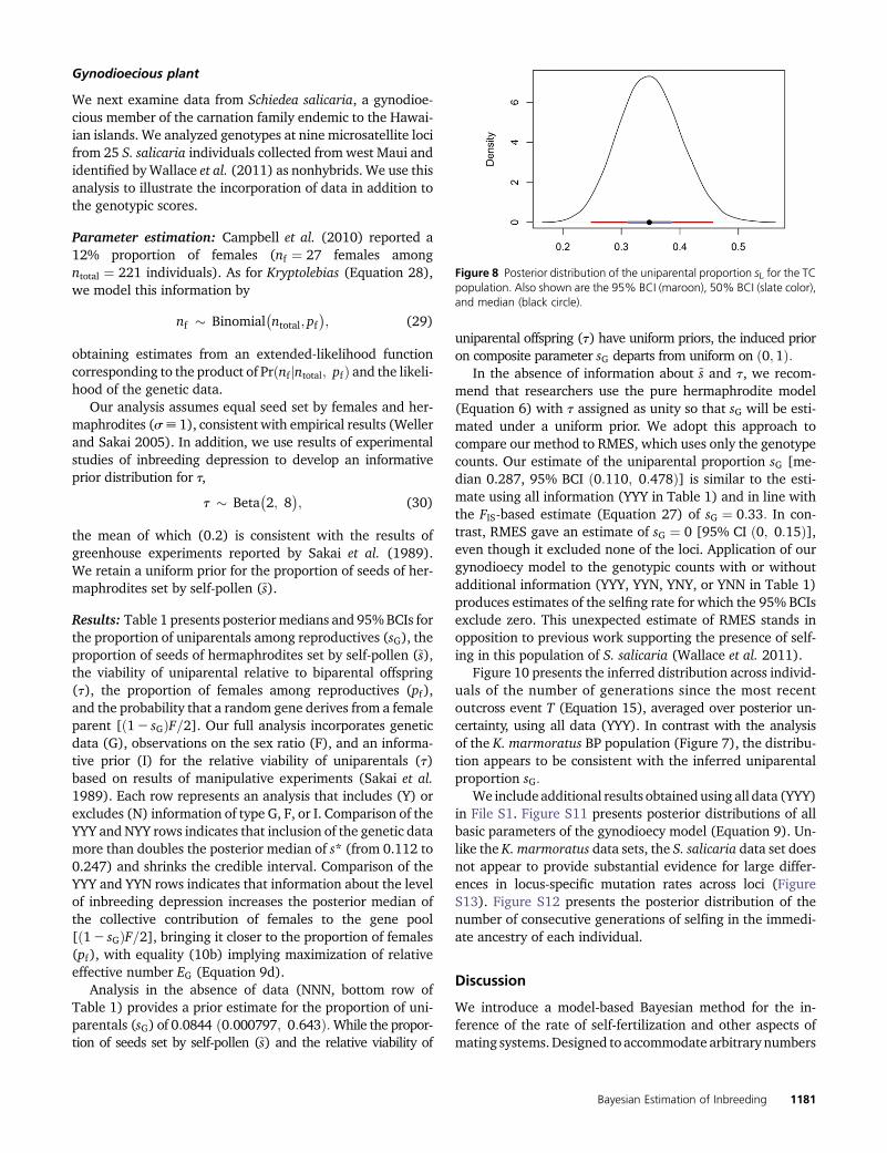
All three methods confirm the inference of Mackiewiczet al. (2006) of much lower inbreeding in the TC populationrelative to the BP population. Our posterior distribution ofuniparental proportion sL has a median and 95% BCI of0:35  ð0:25;   0:45Þ (Figure 8). This median again lies betweenthe FIS-based estimate (Equation 27) of 0.39 and the RMESestimate of 0.33, which has a 95% C.I. of ð0:30;   0:36Þ: In thiscase, RMES excluded from the analysis only a single locus,which was monomorphic in the sample.

Figure 9 shows the inferred distribution of the numberof generations since the most recent outcross event (T)across individuals, averaged over posterior uncertainty. Incontrast to the BP population, the distribution of time sincethe most recent outcross event in the TC population ap-pears to conform to the distribution expected under theinferred uniparental proportion (sL), including a high frac-tion of biparental individuals (Tk ¼ 0). Figure S7 presentsthe posterior distribution of the number of consecutivegenerations of selfing in the immediate ancestry of eachindividual.

Figure 7 Empirical distribution of number of generations since the most recent outcross event (T) across individuals for the BP population of K.marmoratus, averaged across posterior samples. The right panel is constructed by zooming in on the panel on the left. “Expected” probabilitiesrepresent the proportion of individuals with the indicated number of selfing generations expected under the median uniparental proportion sL:“Inferred” probabilities represent proportions inferred across individuals in the sample. The first inferred bar with positive probability corresponds toT ¼ 1:

1180 B. D. Redelings et al.

Gynodioecious plant

We next examine data from Schiedea salicaria, a gynodioe-cious member of the carnation family endemic to the Hawai-ian islands. We analyzed genotypes at nine microsatellite locifrom 25 S. salicaria individuals collected from west Maui andidentified byWallace et al. (2011) as nonhybrids. We use thisanalysis to illustrate the incorporation of data in addition tothe genotypic scores.

Parameter estimation: Campbell et al. (2010) reported a12% proportion of females (nf ¼ 27 females amongntotal ¼ 221 individuals). As for Kryptolebias (Equation 28),we model this information by

nf � Binomial�ntotal; pf

�; (29)

obtaining estimates from an extended-likelihood functioncorresponding to the product of Prðnf jntotal;   pfÞ and the likeli-hood of the genetic data.

Our analysis assumes equal seed set by females and her-maphrodites (s[ 1), consistent with empirical results (Wellerand Sakai 2005). In addition, we use results of experimentalstudies of inbreeding depression to develop an informativeprior distribution for t,

t � Beta�2;   8

�; (30)

the mean of which (0.2) is consistent with the results ofgreenhouse experiments reported by Sakai et al. (1989).We retain a uniform prior for the proportion of seeds of her-maphrodites set by self-pollen (~s).

Results: Table 1 presents posteriormedians and 95%BCIs forthe proportion of uniparentals among reproductives (sG), theproportion of seeds of hermaphrodites set by self-pollen (~s),the viability of uniparental relative to biparental offspring(t), the proportion of females among reproductives (pf ),and the probability that a random gene derives from a femaleparent [ð12 sGÞF=2]. Our full analysis incorporates geneticdata (G), observations on the sex ratio (F), and an informa-tive prior (I) for the relative viability of uniparentals (t)based on results of manipulative experiments (Sakai et al.1989). Each row represents an analysis that includes (Y) orexcludes (N) information of type G, F, or I. Comparison of theYYY and NYY rows indicates that inclusion of the genetic datamore than doubles the posterior median of s* (from 0.112 to0.247) and shrinks the credible interval. Comparison of theYYY and YYN rows indicates that information about the levelof inbreeding depression increases the posterior median ofthe collective contribution of females to the gene pool[ð12 sGÞF=2], bringing it closer to the proportion of females(pf ), with equality (10b) implying maximization of relativeeffective number EG (Equation 9d).

Analysis in the absence of data (NNN, bottom row ofTable 1) provides a prior estimate for the proportion of uni-parentals (sG) of 0:0844  ð0:000797;   0:643Þ:While the propor-tion of seeds set by self-pollen (~s) and the relative viability of

uniparental offspring (t) have uniform priors, the induced prioron composite parameter sG departs from uniform on ð0; 1Þ:

In the absence of information about ~s and t, we recom-mend that researchers use the pure hermaphrodite model(Equation 6) with t assigned as unity so that sG will be esti-mated under a uniform prior. We adopt this approach tocompare our method to RMES, which uses only the genotypecounts. Our estimate of the uniparental proportion sG [me-dian 0.287, 95% BCI ð0:110;   0:478Þ] is similar to the esti-mate using all information (YYY in Table 1) and in line withthe FIS-based estimate (Equation 27) of sG ¼ 0:33: In con-trast, RMES gave an estimate of sG ¼ 0 [95% CI ð0;   0:15Þ],even though it excluded none of the loci. Application of ourgynodioecy model to the genotypic counts with or withoutadditional information (YYY, YYN, YNY, or YNN in Table 1)produces estimates of the selfing rate for which the 95% BCIsexclude zero. This unexpected estimate of RMES stands inopposition to previous work supporting the presence of self-ing in this population of S. salicaria (Wallace et al. 2011).

Figure 10 presents the inferred distribution across individ-uals of the number of generations since the most recentoutcross event T (Equation 15), averaged over posterior un-certainty, using all data (YYY). In contrast with the analysisof the K. marmoratus BP population (Figure 7), the distribu-tion appears to be consistent with the inferred uniparentalproportion sG:

We includeadditional results obtainedusing all data (YYY)in File S1. Figure S11 presents posterior distributions of allbasic parameters of the gynodioecy model (Equation 9). Un-like the K. marmoratus data sets, the S. salicaria data set doesnot appear to provide substantial evidence for large differ-ences in locus-specific mutation rates across loci (FigureS13). Figure S12 presents the posterior distribution of thenumber of consecutive generations of selfing in the immedi-ate ancestry of each individual.

Discussion

We introduce a model-based Bayesian method for the in-ference of the rate of self-fertilization and other aspects ofmating systems. Designed to accommodate arbitrary numbers

Figure 8 Posterior distribution of the uniparental proportion sL for the TCpopulation. Also shown are the 95% BCI (maroon), 50% BCI (slate color),and median (black circle).

Bayesian Estimation of Inbreeding 1181

of loci, it uses the ESF to determine likelihoods in a compu-tationally efficient manner from frequency spectra of geno-types observed at multiple unlinked sites throughout thegenome. Our MCMC sampler explicitly incorporates the fullset of parameters for each mating system considered (purehermaphroditism, Kryptolebias, and gynodioecy). This con-struction permits incorporation of information in addition togenetic data, affording insight into components of the evolu-tionary process beyond the estimation of selfing rates alone.

Components of inference

Locus-specific mutation rates:Ourmethodpermits variationamong loci in the rate of mutation (Equation 3) by using theDPP todetermine thenumberof rate classes, themutation rateof each class, and the class to which each locus belongs. OurDPP adopts a conservative approach, creating a new rate classonly if thedatademand it.Under theDPP, loci belonging to thesame group have identical mutation rates. This approachmightbegeneralized, for example, byusingaDirichlet processmixture to allow variation in mutation rate among loci withina rate class.

Joint inference of mutation and inbreeding rates: For theinfinite-alleles model of mutation, the ESF (Ewens 1972)provides the probability of any allele frequency spectrum(AFS) observed at a locus in a sample derived from a panmic-tic population. Under partial self-fertilization, the ESF pro-vides the probability of an AFS observed among genes, eachsampled from a distinct individual. For such genic (as op-posed to genotypic) samples, the coalescence process underinbreeding is identical to the standard coalescence process,but with a rescaling of time (Fu 1997; Nordborg and Don-nelly 1997). Accordingly, genic samples may serve as thebasis for the estimation of the single parameter of the ESF,the scaled mutation rate u* (Equation 5), but not the rate ofinbreeding apart from the scaled mutation rate.

Our method uses the information in a genotypic sample,the genotype frequency spectrum, to infer both the unipa-rental proportion s* and the scaled mutation rate u*: Our

sampler reconstructs the genealogical history of a sample ofdiploid genotypes only to the point of the most recent ran-dom-outcross event of each individual, with the number ofconsecutive generations of inbreeding in the immediate an-cestry of a given individual (Tk for individual k) correspond-ing to a latent variable in our Bayesian inference framework.Invocation of the ESF beyond the point at which all lineagesreside in separate individuals obviates the necessity of furthergenealogical reconstruction. As a consequence, our methodmay be better able to accommodate genome-scale magni-tudes of observed loci (L).

Identity disequilibrium (Cockerham and Weir 1968), thecorrelation in heterozygosity across loci within individuals,reflects that all loci within an individual experience the mostrecent random-outcross event at the same time, irrespectiveof physical linkage. The heterozygosity profile of individual kprovides information about Tk (Equation 15), which in turnreflects the uniparental proportion s*: Observation of multi-ple individuals provides a basis for inference of both the uni-parental proportion s* and the scaled mutation rate u*:

Estimation of the selfing rate

Accuracy and uncertainty: Enjalbert and David (2000) andDavid et al. (2007) base estimates of selfing rate on the dis-tribution of numbers of heterozygous loci. Bothmethods stripgenotype information from the data, distinguishing betweenonly homozygotes and heterozygotes, irrespective of the al-leles involved. Loci lacking heterozygotes altogether (even ifpolymorphic) are removed from the analysis as uninforma-tive about the magnitude of departure from Hardy–Weinbergproportions (Figure 3). As the observation of polymorphicloci with low heterozygosity provides strong evidence of in-breeding, exclusion of such loci by RMES (David et al. 2007)may contribute to its loss of accuracy for high rates of selfing(Figure 2).

Our method derives information from all loci. Like mostcoalescence-based models, it accounts for the level of varia-tion aswell as theway inwhich variation is partitionedwithinthe sample. Even a locus monomorphic within a sampleprovides information about the age of the most recent

Figure 10 Empirical distribution of selfing times T across individuals, forS. salicaria. The histogram is averaged across posterior samples.

Figure 9 Empirical distribution of selfing times T across individuals, for K.marmoratus (population TC). The histogram is averaged across posteriorsamples.

1182 B. D. Redelings et al.

common ancestor of the observed sequences, a property thatwas not widely appreciated prior to analyses of the absence ofvariation in a sample of human Y chromosomes (Dorit et al.1995; Fu and Li 1996).

Both RMES and our method invoke independence of ge-nealogical histories of unlinked loci, conditional on the timesince the most recent outcrossing event. RMES seeks toapproximate the likelihood by summing over the distributionof time since themost recent outcross event, but truncates theinfinite sum at 20 generations. The increased error exhibitedby RMES under high rates of inbreeding may reflect that thelikelihood has a substantial mass beyond the truncation pointin such cases. Our method explicitly estimates the latentvariable of time since the most recent outcross for each indi-vidual (Equation 13). This quantity ranges over the nonneg-ative integers, but values assigned to individuals are exploredby the MCMC according to their effects on the likelihood.

Estimates of the proportion of uniparental individuals s*(Equation 4) produced by ourmethod appear to show greateraccuracy than RMES over much of the parameter range (Fig-ure 2). Even so, we note that all methods considered hereprovide fair estimates of the selfing rate, including theFIS-based method (Equation 27) that uses only the single-locus departures from Hardy–Weinberg proportions and notidentity disequilibrium. However, our Bayesian method ap-pears to provide a more accurate assessment of uncertaintythan does the maximum-likelihood method RMES: ourBCIs have good frequentist coverage properties (Figure S5),while the C.I.’s reported by RMES appear to perform less well(Figure 4).

Identifiability: In an analysis based solely on the genotypefrequency spectrum observed in a sample, the likelihooddepends on just two composite parameters: the probabilitythat a random individual is uniparental (s*) and the scaledrates of mutation Q* (Equation 19) across loci. Even so, ourMCMC implementation updates the full set of basic parame-ters, with likelihoods determined from the implied values ofs* and Q*:

Any model for which the parameter set C (Equation 23)comprises more than one parameter is not fully identifiablefrom the genetic data alone. In the pure hermaphroditismmodel (Equation 6), for example, basic parameters~s (fraction

of fertilizations by selfing) and t (relative viability of unipa-rental offspring) are nonidentifiable: any assignments thatdetermine the same values of composite parameters s* andQ* have the same likelihood.

For each basic parameter in C beyond one, identifiabilityrequires incorporation of additional information beyond thegenetic data. A full treatment of such information requiresexpansion of the likelihood function to encompass an explicitmodel of the new information. For example, the Kryptolebiasmodel (Equation 7) comprises three basic parameters, in-cluding pm (Equation 8a), the frequency of males amongreproductives. In our analysis of microsatellite data fromthe killifishK.marmoratus (Mackiewicz et al. 2006; Tatarenkovet al. 2012), the expanded-likelihood function corresponds tothe product of the probability of the genetic data and theprobability of the number of males observed among a totalnumber of individuals (Equation 28). In a similarmanner, ouranalysis of the data set from S. salicaria (Wallace et al. 2011)uses an extended-likelihood function that models the ob-served number of females as a binomial random variable(Equation 29), permitting estimation of the frequency of fe-males among reproductives (pf ).

Nonidentifiable parameters can also be estimated throughthe incorporationof informative priors. Because identifiabilityis defined in terms of the likelihood, which is unaffected bypriors, such parameters remain nonidentifiable. Even so, in-formative priors assist in their estimation through Bayesianapproaches, which do not require parameters to be identifi-able. Our analysis of the Schiedea data draws on experimentalevidence in addition to the genotype counts to justify theassumption of equal seed set by females and hermaphrodites(s[ 1) (Weller and Sakai 2005) and to develop an informa-tive prior for t (Equation 30) (Sakai et al. 1989).

Guidance for applying the method: Our present implemen-tation of the method introduced here includes default priorsfor the basic parameters, with users encouraged to specifypriors appropriate for their systems. For example, a biologi-cally motivated prior for the relative viability of uniparentals(t) might favor weak selection (t � 1) or inbreeding depres-sion of an intensity sufficient to maintain selfing (t$ 1=2).

In the Kryptolebiasmodel (Equation 7), comprising basic pa-rameters~s (proportion of eggs self-fertilized by hermaphrodites),

Table 1 Parameter estimates for different amounts of data

G F I sG ~s t pf ð12 sGÞF=2Y Y Y 0:247  ð0:0791; 0:444Þ 0:695  ð0:299;0:971Þ 0:215  ð0:0597;0:529Þ 0:125  ð0:0849;0:173Þ 0:118  ð0:054;0:258ÞY Y N 0:267  ð0:0951; 0:469Þ 0:497  ð0:187; 0:93Þ 0:507  ð0:082; 0:973Þ 0:125  ð0:0851;0:174Þ 0:0808  ð0:0398;0:191ÞY N Y 0:213  ð0:045; 0:402Þ 0:742  ð0:379;1:00Þ 0:252  ð0:0488;0:529Þ 0:244  ð0:00; 0:613Þ 0:218  ð0:0;0:403ÞY N N 0:243  ð0:0608; 0:429Þ 0:628  ð0:268; 0:999Þ 0:611  ð0:167;1:00Þ 0:354  ð0:00; 0:072Þ 0:223  ð0:00; 0:394ÞN Y Y 0:112  ð0:0026; 0:588Þ 0:496  ð0:0252; 0:974Þ 0:183  ð0:0277;0:513Þ 0:125  ð0:0847;0:173Þ 0:0956  ð0:0427;0:218ÞN Y N 0:231  ð0:00391;0:776Þ 0:504  ð0:025; 0:973Þ 0:493  ð0:0257;0:975Þ 0:125  ð0:0847;0:173Þ 0:0778  ð0:0392;0:172ÞN N Y 0:0376  ð0:00;0:318Þ 0:492  ð0:0122; 0:957Þ 0:0:185  ð0:00917; 0:462Þ 0:483  ð0:00; 0:946Þ 0:314  ð0:0361; 0:500ÞN N N 0:0844  ð0:000; 0:643Þ 0:497  ð0:0244; 0:975Þ 0:494  ð0:0252;0:975Þ 0:479  ð0:0245;0:972Þ 0:289  ð0:0313;0:5ÞEstimates are given by a posterior median and a 95% BCI. Each row represents an analysis that includes (Y) or excludes (N) information, including genotype frequency data(G), counts of females (F), and replacement of the Uniform(0,1) prior on t by an informative prior (I).

Bayesian Estimation of Inbreeding 1183

t (relative viability of uniparentals), and pm (proportion ofmales among reproductives), pm together with sL determinesthe scaling of time (Equation 7c), which depends on ~s and t

only through sL: In the absence of information regarding ~sand t, we recommend assigning t[ 1;which permits estima-tion of sL under the default uniform prior or a user-specifiedprior. This assignment produces estimates that are simplyagnostic concerning the relative influence of ~s and t in de-termining sL:

In the four-parameter gynodioecy model (Equation 26),however, the scaling of time (Equation 9d) depends not onlyon sG (the proportion of uniparentals) and pf (the proportionof females among reproductives), but also on F (the propor-tion of biparental offspring that have a female parent). Be-cause F (Equation 9b) depends on ~s (the proportion of seedsset by self-pollen), information about t affects inference of allbasic parameters. In the absence of information about theintensity of inbreeding depression, we recommend usingthe pure hermaphroditism model (Equation 24) under theassignment t[ 1; which permits estimation of the uniparen-tal proportion s* under a uniform prior.

Beyond estimation of the selfing rate

Unlike the other methods considered here, our method pro-vides a framework for the incorporation of information inaddition to counts of diploid genotypes and the inference of anumber of aspects of the mating system beyond the selfingrate.

Time since the most recent outcross: Our method incorpo-rates as a latent variable Tk (Equation 13), the number ofgenerations since the most recent outcross event in the im-mediate ancestry of individual k, and provides posterior dis-tributions for this quantity.

This aspect of the mating system is of biological interest initself and also affords insight into the suitability of the un-derlyingmodel. Pooling suchestimates of times since themostrecent outcross over individuals produces an empirical distri-bution of the number of consecutive generations of selfing.Under the assumption of a single population-wide rate of self-fertilization, we expect selfing time to have a geometricdistribution with parameters corresponding to the estimatedselfing rate. Empirical distributions of the estimated numberof generations since the last outcross appear consistent withthis expectation for the data sets derived from the TC pop-ulation of K. marmoratus (Figure 9) and from Schiedea(Figure 10). In contrast, the empirical distribution for thehighly inbred BP population of K. marmoratus (Figure 7)shows an absence of individuals formed by random outcross-ing (T ¼ 0).

That our method accurately estimates T from simulateddata (Figure 5) argues against attributing the inferred defi-ciency of biparental individuals in the BP data set to an arti-fact of the method. Rather, the deficiency may indicate adeparture from the underlying model, which assumes repro-duction only through self-fertilization or random outcrossing.

In particular, biparental inbreeding as well as selfing mayreduce the fraction of individuals formed by random out-crossing. Misscoring of heterozygotes as homozygotes dueto null alleles or other factors, a possibility directly addressedby RMES (David et al. 2007) but not by our method, may alsoin principle contribute to the apparent deficiency of individ-uals formed by random outcrossing.

Relative effective number: Incorporation of additional in-formation, either through extension of the likelihood orthrough informative priors, permits inference not only ofthe basic parameters but also of functions of the basic param-eters. For example, Table 1 includes estimates of the propor-tion of seeds of hermaphrodites set by self-pollen (~s) and theprobability that a random gene derives from a female parent[ð12 sGÞF=2] in gynodioecious S. salicaria. We are not awareof other studies in which these quantities have been inferredfrom the pattern of neutral genetic variation observed in arandom sample.

Among themost biologically significant functions towhichthis approach affords access is relative effective number E(Equation 3), a fundamental component of the reproductivevalue of the sexes (Fisher 1958). We denote the probabilitythat a pair of genes, randomly drawn from distinct individu-als, derive from the same parent in the preceding generationas the rate of parent sharing (1=N*). Its inverse (N*) corre-sponds to the inbreeding effective size of Crow andDenniston(1988). Relative effective number E is the ratio of N* to thetotal number of reproductive individuals. For example, in theabsence of inbreeding (s* ¼ 0), N* in our gynodioecy model(Equation 9) corresponds to Wright’s (1969) harmonic meanexpression for effective population size and E to the ratio ofN* and Nf þ Nh; the total number of reproductive femalesand hermaphrodites. In general (s*$ 0), relative effectivesize E reflects reductions in effective size due to inbreedingin addition to differences in numbers of the sexual forms.

Figure 11 presents posterior distributions of E for the threedata sets explored here. These results suggest that relativeeffective number E in each of the natural populations sur-veyed lies close to its maximum of unity, with the effectivenumber defined through the rate of parent sharing approach-ing the total number of reproductives. Our estimates suggest

Figure 11 Posterior distributions of relative effective number E (Equation3) for data sets derived from K. marmoratus (BP and TC populations) andS. salicaria.

1184 B. D. Redelings et al.

that maximization of relative effective number would occurunder a slight increase in the frequency of males pm (Equa-tion 8b) in both K. marmoratus populations and a very slightdecrease in the frequency of females pf (Equation 10b) in theS. salicaria population.

Acknowledgments

We thank the Reviewers, Associate Editor Rasmus Nielsen,and Senior Editor John Wakeley for valuable comments andsuggestions. This project was initiated during a sabbaticalvisit of M.K.U. to the Department of Ecology and Evolution-ary Biology at the University of California at Irvine. Wethank Francisco J. Ayala for exceedingly gracious hospitalityand Diane R. Campbell and all members of the Departmentfor stimulating interactions. We thank Lisa E. Wallace formaking available to us microsatellite data from S. salicaria.Public Health Service grant GM 37841 (to M.K.U.) providedpartial funding for this research.

Literature Cited

Ayres, K. L., and D. J. Balding, 1998 Measuring departures fromHardy-Weinberg: a Markov chain Monte Carlo method for esti-mating the inbreeding coefficient. Heredity 80: 769–777.

Campbell, D. R., S. G. Weller, A. K. Sakai, T. M. Culley, P. N. Danget al., 2010 Genetic variation and covariation in floral alloca-tion of two species of Schiedea with contrasting levels of sexualdimorphism. Evolution 65: 757–770.

Clegg, M. T., 1980 Measuring plant mating systems. Bioscience30: 814–818.

Cockerham, C. C., and B. S. Weir, 1968 Sib mating with twolinked loci. Genetics 60: 629–640.

Crow, J. F., and C. Denniston, 1988 Inbreeding and variance ef-fective population numbers. Evolution 42: 482–495.

David, P., B. Pujol, F. Viard, V. Castella, and J. Goudet,2007 Reliable selfing rate estimates from imperfect populationgenetic data. Mol. Ecol. 16: 2474–2487.

Dorit, R. L., H. Akashi, and W. Gilbert, 1995 Absence of polymor-phism at the ZFY locus on the human Y chromosome. Science286: 1183–1185.

Enjalbert, J., and J. L. David, 2000 Inferring recent outcrossingrates using multilocus individual heterozygosity: application toevolving wheat populations. Genetics 156: 1973–1982.

Ewens, W. J., 1972 The sampling theory of selectively neutralalleles. Theor. Popul. Biol. 3: 87–112.

Fisher, R. A., 1958 The Genetical Theory of Natural Selection, Ed. 2.Dover, New York.

Fu, Y.-X., 1997 Coalescent theory for a partially selfing popula-tion. Genetics 146: 1489–1499.

Fu, Y.-X., and W.-H. Li, 1996 Absence of polymorphism at the ZFYlocus on the human Y chromosome. Science 272: 1356–1357.

Furness, A. I., A. Tatarenkov, and J. C. Avise, 2015 A genetic testfor whether pairs of hermaphrodites can cross-fertilize in a self-ing killifish. J. Hered. DOI:10.1093/jhered/esv077.

Gao, H., S. Williamson, and C. D. Bustamante, 2007 A Markovchain Monte Carlo approach for joint inference of population

structure and inbreeding rates from multilocus genotype data.Genetics 176: 1635–1651.

Griffiths, R. C., and S. Lessard, 2005 Ewens’ sampling formulaand related formulae: combinatorial proofs, extensions to vari-able population size and applications to ages of alleles. Theor.Popul. Biol. 68: 167–177.

Haldane, J., 1924 A mathematical theory of natural and artificialselection. Part ii. The influence of partial self-fertilization, in-breeding, assortative mating, and selective fertilization on thecomposition of Mendelian populations, and on natural selection.Biol. Rev. Camb. Philos. Soc. 1: 158–163.

Hill, W. G., H. A. Babiker, L. C. Ranford-Cartwright, and D. Walliker,1995 Estimation of inbreeding coefficients from genotypicdata on multiple alleles, and application to estimation of clon-ality in malaria parasites. Genet. Res. 65: 53–61.

Karlin, S., and J. McGregor, 1972 Addendum to a paper of W.Ewens. Theor. Popul. Biol. 3: 113–116.

Liu, J. S., 2001 Monte Carlo Strategies in Scientific Computing.Springer, New York.

Mackiewicz, M., A. Tatarenkov, D. S. Taylor, B. J. Turner, and J. C.Avise, 2006 Extensive outcrossing and androdioecy in a verte-brate species that otherwise reproduces as a self-fertilizing her-maphrodite. Proc. Natl. Acad. Sci. USA 103: 9924–9928.

Neal, R. M., 2000 Markov chain sampling methods for Dirichletprocess mixture models. J. Comput. Graph. Stat. 9: 249–265.

Nordborg, M., and P. Donnelly, 1997 The coalescent process withselfing. Genetics 146: 1185–1195.

Pritchard, J. K., M. Stephens, and P. Donnelly, 2000 Inference ofpopulation structure using multilocus genotype data. Genetics155: 945–959.

Ritland, K., 2002 Extensions of models for the estimation of mat-ing systems using n independent loci. Heredity 88: 221–228.

Sakai, A. K., K. Karoly, and S. G. Weller, 1989 Inbreeding depres-sion in Schiedea globosa and S. salicaria (Caryophyllaceae), sub-dioecious and gynodioecious Hawaiian species. Am. J. Bot. 76:437–444.

Tatarenkov, A., R. L. Earley, D. S. Taylor, and J. C. Avise,2012 Microevolutionary distribution of isogenicity in a self-fertilizing fish (Kryptolebias marmoratus) in the Florida Keys.Integr. Comp. Biol. 52: 743–752.

Turner, B. J., W. P. Davis, and D. S. Taylor, 1992 Abundant malesin populations of a selfing hermaphrodite fish, Rivulus marmor-atus, from some Belize cays. J. Fish Biol. 40: 307–310.

Wallace, L. E., T. M. Culley, S. G. Weller, A. K. Sakai, A. Kuenziet al., 2011 Asymmetrical gene flow in a hybrid zone of Ha-waiian Schiedea (Caryophyllaceae) species with contrastingmating systems. PLoS One 6: e24845.

Wang, J., Y. A. El-Kassaby, and K. Ritland, 2012 Estimating selfingrates from reconstructed pedigrees using multilocus genotypedata. Mol. Ecol. 21: 100–116.

Weir, B. S., 1996 Genetic Data Analysis II. Sinauer Associates,Sunderland, MA.

Weller, S. G., and A. K. Sakai, 2005 Inbreeding and resource al-location in Schiedea salicaria (Caryophyllaceae), a gynodioe-cious species. J. Evol. Biol. 18: 301–308.

Wright, S., 1921 Systems of mating. I, II, III, IV, V. Genetics 6:111–178.

Wright, S., 1969 The Theory of Gene Frequencies (Evolution andthe Genetics of Populations, Vol. 2). University of Chicago Press,Chicago.

Communicating editor: R. Nielsen

Bayesian Estimation of Inbreeding 1185

Appendix A

The Last-Sampled Gene

We present a first-principles derivation (not requiring knowledge of the ESF) of the probability that the last-sampled gene of igenes randomly sampled from distinct individuals represents a novel allele (Equation 21a).

Under the infinite-allelesmodelofmutation, a singlemutation ina lineage suffices todistinguishanewallele.Wedesignateasthe focal gene the last-sampledgeneand consider the level of the genealogical tree inwhich its ancestral lineage either receives amutation or joins the gene tree of the sample at size ði2 1Þ: Level ℓ of the entire (i-gene) gene tree corresponds to the segment inwhich ℓ lineages persist.

The probability that the line of descent of the focal gene terminates in a mutation immediately, in level i of the genealogy, is

u

iuþ�

i2

��N*�22 s*

� ¼ u*i�u*þ   i2 1

�:In general, the probability that the lineage of the focal gene terminates on level ℓ. 2 is

�i2 1

�uþ

i2 1

2

!,N*�22 s*

�iuþ

i

2

!,N*�22 s*

��i2 2

�uþ

i2 2

2

!,N*�22 s*

��i2 1

�uþ

i2 1

2

!,N*�22 s*

�

. . .  

luþ

l

2

!,N*�22 s*

��lþ 1

�uþ

lþ 1

2

!,N*�22 s*

� u

luþ

l

2

!,N*�22 s*

�¼ u*

i�u*þ i2 1

�:This expression illustrates the invariance over termination orders noted by Griffiths and Lessard (2005). Summing over alllevels, including level 2, for which a mutation in either remaining lineage ensures that the focal gene represents a novel allele,we obtain the overall probability that the last-sampled gene represents a novel allele:

u*�i2 2

�i�u*þ i2 1

�þ 2u*i�u*þ i21

� ¼ u*u*þ i2 1

:

Appendix B

Estimators of FIS

We follow Weir (1996) in developing an estimate of the uniparental proportion s* from FIS alone (Equation 27).For a single locus, a simple estimator of FIS corresponds to

cFIS ¼ 12OE;

for O the observed fraction of heterozygotes in the sample and E the expected fraction based on Hardy–Weinberg proportionsgiven the observed allele frequencies. Explicitly, we have

cFIS ¼ 1212

Xu~Puu

12X

u~p2u

¼�X

u~Puu 2 ~p2u

�12

Xu~p2u

;

for ~pu the frequency of allele u in the sample and ~Puu the frequency of homozygous genotype uu in the sample. However, thisestimator can be substantially biased for small samples, leading to underestimation of FIS (Weir 1996).

To address this bias and accommodate multiple loci, we instead adopt

1186 B. D. Redelings et al.

cFIS ¼XL

l¼1

hXKl

u¼1

�~Pluu 2 ~p2lu

�þ�12

XKl

u¼1~Pluu

�.2ni

XL

l¼1

h�12

XKl

u¼1~p2lu�2�12

XKl

u¼1~Pluu

�.2ni ; (B1)

for n the number of diploid genotypes observed, L the number of loci, and Kl the number of alleles at locus l. While thisestimator is also biased in general, it corresponds to the ratio of unbiased estimators of FIS �

Plð12

Pup

2luÞ and

Plð12

Pup

2luÞ;

in which plu is the frequency of allele u at locus l in the entire population (Weir 1996). Our analysis of simulated data (AppendixD) indicates that this estimator is more accurate than an estimator that simply averages single-locus estimates:

cFIS ¼ 1L

XLl¼1

XKl

u¼1

�~Pluu 2 ~p2lu

�þ�12

XKl

u¼1~Pluu

�.2n�

12XKl

u¼1~p2lu�2�12

XKl

u¼1~Pluu

�.2n

: (B2)

Our FIS-based estimates (Equation 27) incorporate (B1) and not (B2).

Appendix C

Implementation of the MCMC

State space

The state space for the Markov chain of our MCMC sampler includes times across sampled individuals since the last outcrossevent T (Equation 13), coalescence events across individuals and loci since that event I (Equation 14), and model-specificparameters C (Equation 23). The state space also comprises the scaled mutation rates Q* (Equation 19), which are de-termined by C; a list specifying the mutation rate category Cl for locus l ¼ 1 . . . L; and Z; a list specifying the scaled mutationrate Zi for category i ¼ 1 . . . Lþ 4: For example, the scaled mutation rate at locus l corresponds to

u*l ¼ ZCl : (C1)

While the actual number of observed rate categories does not exceed the number of loci (L), expanding the size of the lists toLþ 4 improves mixing of the MCMC by ensuring that multiple categories are available for the placement of a new, previouslyunobserved category (see section 6 of Neal 2000). At any given point in the MCMC, the state of the Markov chain correspondsto ðI;T;C;C;ZÞ:Iterations

Each iteration of our MCMC sampler performs multiple updates, with each variable updated at least once per iteration. Werecorded the state sampled by the MCMC at each iteration. We assessed convergence by computing for each parameter aneffective number of independent samples [effective sample size (Liu 2001)]. Effective numbers for the large sample regimeexceeded 500 samples for each parameter on average, while effective number for the small sample regime exceeded 250samples for each parameter on average. We found that 2000 iterations were more than sufficient to achieve these effectivenumbers. About 14.5 min were required to complete 2000 iterations for the large sample regime on a Core i3–4030 processor;�10 sec were required for the small sample regime.

Foranalysesof simulateddata sets,we ranMarkovchains for2000 iterations, discarding thefirst 200 iterationsasburn-in. Foranalyses of the actual data sets, we ran Markov chains for 100,000 iterations, discarding the first 10,000 iterations as burn-in.Convergence appeared to occur as rapidly for actual data as for simulated data, butwe found empirically that the larger numberof samples was needed to achieve smooth density plots for the actual data sets.

Transition kernels

Updating of the continuous variables ofmutation rates fZlg (Equation C1) andmodel-specific parametersC (Equation 23) usesboth Metropolis–Hastings (MH) transition kernels and autotuned slice-sampling transition kernels. Updating of the discretevariables fClg uses a Gibbs transition kernel.

Efficient inference on selfing times through collapsed Metropolis–Hastings

SimpleMHproposals that separately update the time since themost recent outcross event (Tk) andcoalescencehistory since thatevent (I�k) lead to extremely poor mixing efficiency. Strong correlations between Tk and I�k cause changes to Tk to be rejectedwith high probability unless I�k is updated as well. For example, consider proposing a change of Tk from 1 to 0.When Tk ¼ 1; onaverage Ilk will be 1 at half of the loci and 0 at the remaining loci. If any of the Ilk ¼ 1; a move to Tk ¼ 0 will always be rejected

Bayesian Estimation of Inbreeding 1187

because the probability of a coalescence event more recently than the most recent outcross event is 0 if the sampled individualis itself a product of outcrossing. To permit acceptance of changes to Tk; we introduce a proposal for Tk that also changes I�k:

The scheme starts from the value Tk ¼ tk and proposes a new value t9k: In standard MHwithin Gibbs, we would compute theprobability of Tk ¼ tk and of Tk ¼ t9k given that all other parameters are unchanged. We modify this MH scheme to computeprobabilities without conditioning on the coalescence indicators for individual k. However, the coalescence indicators for otherindividuals are still held constant. To compute this probability, let J indicate all the coalescence indicators I�y where y 6¼ k: Then

Pr�X;T; J; s; u

� ¼ Pr�X; JjT; s; u�Pr�Tjs�Pr�s�Pr�u�:

We introduce I�k by summing over all possible values i�k :

Pr�X; JjT; s; u� ¼X

i�k

Pr�X; I�k ¼ i�k; JjT; s; u

�:

Since the ilk for different loci are independent given Tk; we have

Pr�X; JjT; s; u� ¼P

i�k

QLl¼1

Pr�Xl;   Ilk ¼ ilk; JljT; s; u

�¼ QL

l¼1

Pilk

Pr�Xl; Ilk ¼ ilk; JljT; s; u

�:

Therefore, for specific values of T and J; we can compute the sum over all possible values of I�k for l ¼ 1 . . . L in computationtime proportional to L instead of 2L: This is possible because the L coalescence indicators for individual k each affect differentloci and are conditionally independent given Tk and J:

After accepting or rejecting the new value of Tk with I�k integrated out, we must choose new values for I�k given the chosenvalue of Tk: Because of their conditional independence, we may separately sample each coalescence indicator Ilk for l ¼ 1 . . . Lfrom its full conditional given the chosen value of Tk: This completes the collapsed MH proposal.

Appendix D

Analysis of Simulated Data

Simulations

Our simulator (https://github.com/skumagai/selfingsim) was developed using simuPOP, publicly available at http://simu-pop.sourceforge.net/. It explicitly represents N ¼ 10; 000 individuals, each bearing two genes at each of L unlinked loci.Mutations arise at locus l at scaled rate ul (Equation 3), in accordance with the infinite-alleles model.

We assigned to uniparental proportion s* values ranging from 0.01 to 0.99, with half of the L ¼ 32 loci assigned scaledmutation rate u ¼ 0:5 and the remaining loci assigned u ¼ 1:5:

We conducted 102 independent simulations for each assignment of s*: Each simulation was initialized with each of the2N3 32 genes representing a unique allele. Most of this maximal heterozygosity was lost very rapidly, with allele number andallele frequency spectrum typically stabilizing well within 10N generations. After 20N generations, we recorded the realizedpopulation, from which 100 independent samples of L ¼ 32 loci of size n ¼ 70 were extracted. From this collection, werandomly chose L ¼ 6 loci and subsampled 100 independent samples of size n ¼ 6:

Analysis

We applied our Bayesian method, the FIS method, and RMES to 102 independent samples from each of 102 independentsimulations for each assignment of the uniparental proportion s*: Our Bayesian method is open source and can be obtained athttps://github.com/bredelings/BayesianEstimatorSelfing/. We used the implementation of RMES (David et al. 2007) pro-vided at http://www.cefe.cnrs.fr/images/stories/DPTEEvolution/Genetique/fichiers%20Equipe/RMES%202009%282%29.zip.

1188 B. D. Redelings et al.

GENETICSSupporting Information

www.genetics.org/lookup/suppl/doi:10.1534/genetics.115.179093/-/DC1

A Bayesian Approach to Inferring Rates of Selfingand Locus-Specific Mutation

Benjamin D. Redelings, Seiji Kumagai, Andrey Tatarenkov, Liuyang Wang, Ann K. Sakai,Stephen G. Weller, Theresa M. Culley, John C. Avise, and Marcy K. Uyenoyama

Copyright © 2015 by the Genetics Society of AmericaDOI: 10.1534/genetics.115.179093

File S1

Supporting Information

1 Assessment of the methods

1.1 Comparison of the median of the posterior distribution of the

uniparental proportion

We address the relative accuracy of estimates of the uniparental proportion s∗ produced by

our Bayesian method relative to those produced by RMES and the FIS method (27) upon

application to simulated data (compare Assessment of Accuracy and Coverage using Simu-

lated Data section). While we summarize our posterior distributions of s∗ by the mode in

the main text, we here use the median.

We first address application of the methods to simulated data under the large-sample

regime (n = 70 individuals, L = 32 loci). Except in cases in which the true s∗ is very close

to 0, the error for RMES exceeds the error for our method (Figure S1), a trend that is apparent

under under both the large- and small-sample regimes. The error for the FIS-based estimate

also exceeds the error for our method. It is largest near s∗ = 0 and vanishes as s∗ approaches

1, a pattern distinct from RMES.

Both RMES and our method show positive bias upon application to data sets for which

the true uniparental proportion s∗ is close to zero and negative bias for s∗ close to unity.

This trend reflects that both methods yield estimates of s∗ constrained to lie between 0 and

1. In contrast, the FIS-based estimate (27) underestimates s∗ throughout the range, even

near s∗ = 0 (F̂IS is not constrained to be positive). Our method has a bias near 0 that

is substantially larger than the bias of RMES, and an error that is slightly larger. A major

contributor to this trend is that our Bayesian estimate is represented by only the median of

the posterior distribution of the uniparental proportion s∗.

B. D. Redelings et al. 2 SI

Figure S2 indicates that for data sets generated under a true value of s∗ of 0 (full random

outcrossing), the posterior distribution for s∗ has greater mass near 0. We suggest that the

bias shown near s∗ = 0 merely represents uncertainty in the posterior distribution for s∗ and

not any preference for incorrect values. We note that our method assumes that the data are

derived from a population reproducing through a mixture of self-fertilization and random

outcrossing. Assessment of a model of complete random mating (s∗ = 0) against the present

model (s∗ > 0) might be conducted through the Bayes factor.

Figure S3 indicates that all methods show increased error upon application of smaller

samples (n = 10 individuals, L = 6 loci), as expected. Comparison of our method and RMES

show trends qualitatively similar to the large-sample case: positive bias upon application

to data sets for which the true uniparental proportion s∗ is close to zero and negative bias

for s∗ close to unity, with less error exhibited by our method throughout the range of the

uniparental proportion (s∗).

1.2 Comparison of the median, mode, and mean

In addition to the mode (Figure 2) and median (Figure S1), error might also be assessed by

consideration of the mean of the posterior distribution of s∗. Figure S4 suggests that the

bias and root-mean-squared (rms) error of the mode, median, and mean exhibit different

properties. For example, the posterior mode shows smaller bias throughout the parameter

range, but the median and mean show smaller rms error for s∗ near the boundaries (near 0

or 1). That the posterior mode does not display large bias near s∗ = 0 is consistent with our

suggestion that the larger error of the mean in that region reflects higher uncertainty.

1.3 Frequentist coverage

As for the 95% BCIs (Figure 4), Figure S5 indicates that BCIs of different nominal values

(0.5, 0.75, 0.9, 0.95, and 0.99) display the same pattern, with coverage exceeding the desired

value for intermediate true s∗ values and dipping below the desired value for very high values

B. D. Redelings et al. 3 SI

of s∗. Coverage is closer to the nominal value for the 0.99 and 0.95 levels than for the 0.5

level.

2 Data analysis

2.1 Self-fertilizing vertebrate

Figure S6 shows the posterior distributions of number of generations since the most recent

outcross event (13) for each sampled individual in the highly inbred BP population of K.

marmoratus. Figure S7 shows the posterior distributions for the more outbred TC popula-

tion.

Figures S8 and S9 present posterior distributions of locus-specific mutation rates for the

BP and TC populations, respectively. For each locus, Fig. S10 compares the rank order of

its median mutation rate estimated from the BP data set versus that from the TC data set.

If a relationship exists between the mutation rates estimated from the datasets, it appears

to be diffuse.

2.2 Gynodioecious plant

Figure S11 presents posterior distributions for the uniparental proportion (sG), the propor-

tion of females among reproductives (pf ), the proportion of seeds set by hermaphrodites by

self-pollen (s̃), and the viability of uniparental offspring relative to biparental offspring (τ).

Figure S12 presents the inferred number of generations since the most recent outcross

event Tk (13) for each individual k.

Figure S13 presents posterior distributions for locus-specific mutation rates inferred from

the S. salicaria data set. The loci appear to have similar posterior medians.

B. D. Redelings et al. 4 SI

0.00

0.05

0.10

0.15

0.0 0.2 0.4 0.6 0.8 1.0Selfing rate

Ave

rage

err

or

variable

bias

rms

type

median

RMES

Fis

Figure S1 Errors for the full likelihood (posterior median), RMES, and FIS-based (27)methods for a large simulated sample (n = 70 individuals, L = 32 loci). In the legend,rms indicates the root-mean-squared error and bias the average deviation. Averages aretaken across simulated data sets at each true value of s∗.

B. D. Redelings et al. 5 SI

0

20

40

0.000 0.025 0.050 0.075 0.100s*

Den

sity

Figure S2 Average posterior density of the uniparental proportion (s∗) inferred from simu-lated data generated under the large sample regime (n = 70, L = 32) with a true value ofs∗ = 0. The average was taken across posterior densities for 100 data sets.

B. D. Redelings et al. 6 SI

−0.2

0.0

0.2

0.0 0.2 0.4 0.6 0.8 1.0Selfing rate

Ave

rage

err

or

variable

bias

rms

type

median

RMES

Fis

Figure S3 Errors for the full likelihood (posterior median), RMES, and FIS methods for asmall sample (n = 10 individuals, L = 6 loci). In the legend, rms indicates the root-mean-squared error and bias the average deviation. Averages are taken across simulated datasets at each true value of s∗.

B. D. Redelings et al. 7 SI

0.0

0.1

0.0 0.1 0.2 0.3 0.4 0.5 0.6 0.7 0.8 0.9 1.0Selfing rate

Ave

rage

err

or

variable

bias

rms

type

mean

median

mode

(a) n = 10, L = 6

0.00

0.02

0.04

0.0 0.1 0.2 0.3 0.4 0.5 0.6 0.7 0.8 0.9 1.0Selfing rate

Ave

rage

err

orvariable

bias

rms

type

mean

median

mode

(b) n = 70, L = 32

Figure S4 Errors for the posterior mean, posterior median, and posterior mode. Bluecurves (rms) indicate the root-mean-squared error, and red curves (bias) the average de-viation. Averages are taken across simulated data sets at each true value of the selfing rates∗.

B. D. Redelings et al. 8 SI

●

●

●

●

●

●

●

●

●

●

●

●

●

●

●

●

●

●

●

●

●

●

●

●●

●

●

●

●

●

●

●

●

●

●

●

●

●

●

●

●

●

●

●

●

●

●

●

●

●

●

●

●

●

●

●

●

●

●

●

●

●

●

●

●

●

●

●

●

●

●

●

●

●

●

●

●

●

●

●

●

●

●

●

●

●

●

●

●

●

●

●

●

●

●

●

●

●

●

●

●

●

●

●

●

●

●

●

●

●

●

●

●

●

●

●

●

●

●

●

●

●

●

●

●

●

●

●

●

●

●

●

●

●

●

0.0

0.1

0.2

0.3

0.4

0.5

0.6

0.7

0.8

0.9

1.0

0.0 0.1 0.2 0.3 0.4 0.5 0.6 0.7 0.8 0.9 1.0Selfing rate

Fre

quen

tist c

over

age

CI

●

●

●

●

●

0.5

0.75

0.9

0.95

0.99

Figure S5 Frequentist coverage for Bayesian credible intervals at different levels of credi-bility under the large sampling regime (n = 70, L = 32).

B. D. Redelings et al. 9 SI

● ● ● ● ● ● ● ● ● ● ●

● ● ● ● ● ● ● ● ● ● ● ● ● ● ● ● ● ● ● ● ● ● ● ● ● ● ● ● ●

● ● ● ● ● ● ● ● ● ● ● ● ● ● ● ● ● ● ● ● ● ● ● ● ● ● ● ● ● ● ● ● ● ● ● ● ● ● ● ● ● ● ● ● ● ● ● ● ● ● ● ● ● ● ●

● ● ● ● ● ● ● ● ● ● ● ● ● ● ● ● ● ● ● ● ● ● ● ● ● ● ● ● ● ● ● ● ● ● ● ● ● ● ● ● ● ● ● ● ● ● ● ● ● ● ● ● ●

● ● ● ● ● ● ● ● ● ● ● ● ● ● ● ● ● ● ● ● ● ● ● ● ● ● ● ● ● ● ● ● ● ● ● ● ● ● ● ● ● ● ● ● ● ● ● ● ● ● ● ●

● ● ● ● ● ● ● ● ● ● ● ● ● ● ● ● ● ● ● ● ● ● ● ● ● ● ● ● ● ● ● ● ● ● ● ● ● ● ● ● ● ● ● ● ● ● ● ● ●

● ● ● ● ● ● ● ● ● ● ● ● ● ● ● ● ● ● ● ● ● ● ● ● ● ● ● ● ● ● ● ● ● ● ● ● ● ● ● ● ● ● ● ● ● ● ● ● ●

● ● ● ● ● ● ● ● ● ● ● ● ● ● ● ● ● ● ● ● ● ● ● ● ● ● ● ● ● ● ● ● ● ● ● ● ● ● ● ● ● ● ● ● ● ● ● ●

● ● ● ● ● ● ● ● ● ● ● ● ● ● ● ● ● ● ● ● ● ● ● ● ● ● ● ● ● ● ● ● ● ● ● ● ● ● ● ● ● ● ● ●

● ● ● ● ● ● ● ● ● ● ● ● ● ● ● ● ● ● ● ● ● ● ● ● ● ● ● ● ● ● ● ● ● ● ● ● ● ● ● ● ● ● ● ●

● ● ● ● ● ● ● ● ● ● ● ● ● ● ● ● ● ● ● ● ● ● ● ● ● ● ● ● ● ● ● ● ● ● ● ● ● ● ● ● ● ● ● ●

● ● ● ● ● ● ● ● ● ● ● ● ● ● ● ● ● ● ● ● ● ● ● ● ● ● ● ● ● ● ● ● ● ● ● ● ● ● ● ● ● ● ● ●

● ● ● ● ● ● ● ● ● ● ● ● ● ● ● ● ● ● ● ● ● ● ● ● ● ● ● ● ● ● ● ● ● ● ● ● ● ● ● ● ● ●

● ● ● ● ● ● ● ● ● ● ● ● ● ● ● ● ● ● ● ● ● ● ● ● ● ● ● ● ● ● ● ● ● ● ● ● ● ● ● ● ● ●

● ● ● ● ● ● ● ● ● ● ● ● ● ● ● ● ● ● ● ● ● ● ● ● ● ● ● ● ● ● ● ● ● ● ● ● ● ● ● ● ● ●

● ● ● ● ● ● ● ● ● ● ● ● ● ● ● ● ● ● ● ● ● ● ● ● ● ● ● ● ● ● ● ● ● ● ● ● ● ● ● ● ● ●

● ● ● ● ● ● ● ● ● ● ● ● ● ● ● ● ● ● ● ● ● ● ● ● ● ● ● ● ● ● ● ● ● ● ● ● ● ● ● ● ● ●

● ● ● ● ● ● ● ● ● ● ● ● ● ● ● ● ● ● ● ● ● ● ● ● ● ● ● ● ● ● ● ● ● ● ● ● ● ● ● ● ● ●

● ● ● ● ● ● ● ● ● ● ● ● ● ● ● ● ● ● ● ● ● ● ● ● ● ● ● ● ● ● ● ● ● ● ● ● ● ● ● ● ● ●

● ● ● ● ● ● ● ● ● ● ● ● ● ● ● ● ● ● ● ● ● ● ● ● ● ● ● ● ● ● ● ● ● ● ● ● ● ● ● ● ● ●

● ● ● ● ● ● ● ● ● ● ● ● ● ● ● ● ● ● ● ● ● ● ● ● ● ● ● ● ● ● ● ● ● ● ● ● ● ● ● ● ● ●

● ● ● ● ● ● ● ● ● ● ● ● ● ● ● ● ● ● ● ● ● ● ● ● ● ● ● ● ● ● ● ● ● ● ● ● ● ● ● ● ● ●

● ● ● ● ● ● ● ● ● ● ● ● ● ● ● ● ● ● ● ● ● ● ● ● ● ● ● ● ● ● ● ● ● ● ● ● ● ● ● ● ● ●

● ● ● ● ● ● ● ● ● ● ● ● ● ● ● ● ● ● ● ● ● ● ● ● ● ● ● ● ● ● ● ● ● ● ● ● ● ● ● ● ● ●

● ● ● ● ● ● ● ● ● ● ● ● ● ● ● ● ● ● ● ● ● ● ● ● ● ● ● ● ● ● ● ● ● ● ● ● ● ● ● ● ● ●

● ● ● ● ● ● ● ● ● ● ● ● ● ● ● ● ● ● ● ● ● ● ● ● ● ● ● ● ● ● ● ● ● ● ● ● ● ● ● ● ● ●

● ● ● ● ● ● ● ● ● ● ● ● ● ● ● ● ● ● ● ● ● ● ● ● ● ● ● ● ● ● ● ● ● ● ● ● ● ● ● ● ● ●

● ● ● ● ● ● ● ● ● ● ● ● ● ● ● ● ● ● ● ● ● ● ● ● ● ● ● ● ● ● ● ● ● ● ● ● ● ● ● ● ● ●

● ● ● ● ● ● ● ● ● ● ● ● ● ● ● ● ● ● ● ● ● ● ● ● ● ● ● ● ● ● ● ● ● ● ● ● ● ● ● ● ● ●

● ● ● ● ● ● ● ● ● ● ● ● ● ● ● ● ● ● ● ● ● ● ● ● ● ● ● ● ● ● ● ● ● ● ● ● ● ● ● ● ● ●

● ●

● ● ●

● ● ●

● ● ●

● ● ●

● ● ●

● ● ●

● ● ●

● ● ●

● ● ●

● ● ●

● ● ●

● ● ●

● ● ●

● ● ●

● ● ●

● ● ●

● ● ●

● ● ●

● ● ●

● ● ●

● ● ●

● ● ●

● ● ●

● ● ●

● ● ●

● ● ●

● ● ●

● ● ●

●● ●

● ● ● ●

● ● ● ●

● ● ●

● ● ●

● ● ●

● ● ●

● ● ●

● ● ●

● ● ●

● ● ●

● ● ●

● ● ●

● ● ●

● ● ●

● ● ●

● ● ●

● ● ●

● ● ●

● ● ●

● ● ●

● ● ●

● ● ●

● ● ●

● ● ●

● ● ●

● ● ●

● ● ●

● ● ●

●

●

●

●

●

●

●

●

●

●

●

●

●

●

●

●

●

●

●

●

●

●

●

●

●

●

●

●

●

●

● ●

● ●

● ●

● ●

● ●

● ●

● ●

● ●

● ●

● ●

● ●

● ●

● ●

● ●

● ●

● ●

● ●

● ●

● ●

● ●

● ●

● ●

● ●

● ●

● ●

● ●

● ●

● ●

●

●

●●

●

●

●

●

●

●

●

●

● ●

● ●

● ●

● ●

● ●

● ●

● ●

● ●

● ●

● ●

● ●

● ●

● ●

● ●

● ●

● ●

● ●

● ●

● ●

● ●

● ●

● ●

● ●

● ●

● ●

● ●

● ●

● ●

●

●

●

●

●

●

●

●

●

●

●

●

●

●

●

●

●

●

●

●

●

●

●

●

●

●

●

●

●

●

●

●

●

●

●

●

●

●

●

●

●

●

●

●

●

●

●

●

●

●

●

●

●

●

●

●

●

0

10

20

30

46 18 42 41 45 49 14 32 53 70 4 55 21 29 54 33 40 66 12 6 38 35 27 69 34 1 68 24 15 22 64 28 67 39 51 5 65 11 9 10 2 17 43 62 58 20 52 59 56 47 30 26 16 23 31 25 60 3 19 44 36 63 50 8 61 37 48 7 13 57Individual

Gen

erat

ions

of s

elfin

g

Figure S6 Number of generations since the most recent outcross event in the ancestry ofeach individual in the sample from the BP population of K. marmoratus. The area of eachdot indicates the posterior probability that an individual (X-axis) has the indicated num-ber (Y-axis) of consecutive generations of selfing in its immediate ancestry. The red lineindicates the posterior mean number of selfing generations and the blue line indicates thenumber of heterozygous loci across individuals. The Y-axis is truncated to [0, 30].

B. D. Redelings et al. 10 SI

●●

● ● ● ●●

●

● ● ● ●●●

●

● ●●● ●● ● ●● ●

●

●● ●

●●

● ●● ●

●

● ●● ●

● ●● ● ● ● ● ● ●

● ● ● ● ●● ●

●

●

● ●● ●

● ●●

● ●● ● ●

● ●

●

● ● ●● ●

●●

●

● ● ● ● ●● ● ● ●

● ● ●● ● ●

●

●● ● ●

● ●

●

● ●● ●

●

●

0

10

20

30

2 5 10 12 13 17 20 28 35 36 37 43 48 50 53 55 56 58 3 47 57 38 30 23 54 42 32 49 59 29 26 41 14 40 31 46 39 52 34 33 11 44 21 15 1 6 24 4 51 25 16 19 22 7 18 9 45 8 27Individual

Gen

erat

ions

of s

elfin

g

Figure S7 Number of generations since the most recent outcross event in the ancestry ofeach individual in the sample from the TC population of K. marmoratus. Symbols as inFigure S6.

B. D. Redelings et al. 11 SI

26 18 27 1 5 30 29 31 15 22 20 25 6 28 21 19 2 7 10 16 32 11 12 4 3 14 17 9 13 24 23 8

0.0

2.5

5.0

7.5

10.0

Density

The

ta*

Figure S8 Posterior distributions for mutation rates at each locus in K. marmoratus (BPpopulation). For each distribution. the locus name is indicated in the grey shaded box.

B. D. Redelings et al. 12 SI

26 31 6 5 1 21 7 20 29 14 16 25 18 22 28 32 15 19 4 3 10 27 24 30 12 17 11 2 9 13 23 8

0

10

20

30

Density

The

ta*

Figure S9 Mutation rates at each locus for K. marmoratus (TC population). For eachdistribution. the locus name is indicated in the grey shaded box.

B. D. Redelings et al. 13 SI

●

●

●●

●●

●

●

●

●

●

●

●

●

●

●

●

●

●

●

●

●

●

●

●

●

●

●

●

●

●

●

0

10

20

30

0 10 20 30BP population

TC

pop

ulat

ion

Figure S10 Comparison of rank order of estimated locus-specific mutation rates betweenthe BP and TC populations of K. marmoratus. Each dot represents the rank order of themedian of the mutation rate of a given locus estimated from the BP data set versus thatfrom the TC data set.

B. D. Redelings et al. 14 SI

0.0 0.1 0.2 0.3 0.4 0.5 0.6

01

23

4

Den

sity

●

(a)0.05 0.10 0.15 0.20

05

1015

Den

sity

●

(b)

0.0 0.2 0.4 0.6 0.8 1.0

0.0

0.5

1.0

1.5

2.0

Den

sity

●

(c)0.0 0.2 0.4 0.6 0.8

0.0

1.0

2.0

3.0

Den

sity

●

(d)

Figure S11 Posterior distributions on (a) sG, (b) pf , (c) s̃, and (d) τ for the Schiedea sali-caria data set. Also shown are 95% BCI (maroon), 50% BCI (slate), and median (blackdot).

B. D. Redelings et al. 15 SI

●

●

●

●

●

●

● ●

● ●

● ●

● ● ● ● ●

● ● ● ● ●

● ● ●

●

● ● ● ● ● ● ● ●

● ● ● ● ● ● ● ●

● ● ● ● ●

●

● ● ● ● ● ●

● ● ● ● ● ●

● ● ● ●

●

●

●

●

●

● ●

● ●

● ●

0

2

4

6

18 9 22 14 24 2 10 19 5 12 6 7 8 3 20 23 1 17 4 21 15 16 11 13 25Individual

Gen

erat

ions

of s

elfin

g

Figure S12 Estimated number of selfing generations for each individual for S. salicaria.The area of each dot indicates the posterior probability that a numbered individual (x-axis) has been selfed for a given number of generations (y-axis). For each individual thered line indicates the posterior mean number of selfing generations and the blue line indi-cates the number of heterozygous loci.

B. D. Redelings et al. 16 SI

L6 L2 L4 L7 L8 L3 L5 L9 L1

0.0

0.5

1.0

1.5

2.0

Density

The

ta*

Figure S13 Posterior distributions for mutation rates at locus in S. salicaria. For eachdistribution, the locus name is indicated in the grey shaded box.

B. D. Redelings et al. 17 SI