Real-Time Syst (2012) 48:223–263DOI 10.1007/s11241-011-9144-7

A bandwidth allocation scheme for compositionalreal-time systems with periodic resources

Nathan Fisher · Farhana Dewan

Published online: 20 December 2011© Springer Science+Business Media, LLC 2011

Abstract Allocation of bandwidth among components is a fundamental problem incompositional real-time systems. State-of-the-art algorithms for bandwidth alloca-tion use either exponential-time or pseudo-polynomial-time techniques for exact al-location, or linear-time, utilization-based techniques which may over-provision band-width. In this paper, we propose research into a third possible approach: parametricapproximation algorithms for bandwidth allocation in compositional real-time sys-tems. We develop a fully-polynomial-time approximation scheme (FPTAS) for allo-cating bandwidth for sporadic task systems scheduled by earliest-deadline first (EDF)upon an Explicit-Deadline Periodic (EDP) resource. Our algorithm takes, as parame-ters, the task system and an accuracy parameter ε > 0, and returns a bandwidth whichis guaranteed to be at most a factor (1 + ε) more than the optimal minimum band-width required to successfully schedule the task system. Furthermore, the algorithmhas time complexity that is polynomial in the number of tasks and 1/ε.

Keywords Compositional real-time systems · Schedulability analysis · Periodicresource model · Sporadic tasks · Earliest-deadline first · Approximation algorithms

1 Introduction

Component-based design is widely practiced in system design and development dueto the remarkable benefits obtained from decomposing a complex system into simpler

A preliminary version of this work has been published in 21st Euromicro Conference on Real-TimeSystems, 2009, pages 87–96 (Fisher and Dewan 2009).

N. Fisher (�) · F. DewanDepartment of Computer Science, Wayne State University, 5057 Woodward Avenue, Suite 3010,Detroit, MI, USAe-mail: fishern@cs.wayne.edu

F. Dewane-mail: farhanad@wayne.edu

224 Real-Time Syst (2012) 48:223–263

Fig. 1 An example of resourceallocation in the EDP model

components. Component abstraction, a central goal of component-based design, per-mits each component to hide internal complexity and details from developers of othercomponents and only exposes information necessary to use the component via an in-terface. Recently, component-based design for real-time systems has received consid-erable attention, as numerous frameworks for compositional real-time systems havebeen proposed (for a non-exhaustive list see Deng and Liu 1997; Feng and Mok 2002;Shin and Lee 2008; Albers et al. 2008).

For compositional real-time systems, most proposed frameworks facilitate the ab-straction of each component’s real-time requirements by specifying a real-time in-terface for each component. A real-time interface describes the processing-resourcesupply that a component requires to meet all real-time constraints. Though the vari-ous proposed compositional frameworks differ in the component information that isexposed to the system by a real-time interface, a common necessary attribute is the in-terface bandwidth. The interface bandwidth simultaneously quantifies the fraction ofthe total system resource supply that a component C will require to meet its real-timeconstraints and the component C’s “interference” on the resource supply providedto other system components. Thus, an important fundamental problem in design andanalysis of compositional real-time systems is the minimization of real-time interfacebandwidth (MIB-RT).

Using the notation of Shin and Lee (2008), let component C be characterized by(W,A) where W represents the real-time workload generated by C and A representsthe component-level scheduling algorithm.1 Let I ∈ I denote a real-time interface I

from the set I of all possible real-time interfaces in a given compositional framework.Let β(I) denote the interface bandwidth of real-time interface I . We say the compo-nent C is schedulable upon interface I , if, for any resource supply R that exceeds orequals the resource supply specified by I , W can meet all deadlines when scheduledby A upon R. With these notations, our goal is to minimize interface bandwidth β(I)

for a specific compositional framework: explicit deadline periodic (EDP) (Easwaranet al. 2007) resources.

In the EDP model (Fig. 1), a resource Ω is characterized by a three-tuple(Π,Θ,Δ). The interpretation of such a resource is that a component C executed uponΩ is guaranteed Θ units of processing resource supply for successive Π -length in-tervals (given some initial starting time). Furthermore, the Θ units of resource supplymust be provided within Δ (≤ Π ) time units after the start of the Π -length interval.For Ω = (Π,Θ,Δ), Π is referred to as the period of repetition, Θ is the capacity,

1Note the component-level scheduling algorithm may differ from the system-level scheduling algorithm.Furthermore, many compositional frameworks permit components to be composed of sub-components.

Real-Time Syst (2012) 48:223–263 225

Fig. 2 MIB-RT problem for periodic resources

and Δ is the relative deadline. The EDP model generalized the simpler period re-source model (Shin and Lee 2003) which represented a resource by (Π,Θ) wherethe resource relative deadline is implicit (i.e., Δ = Π ). The advantage of the EDPmodel over the periodic resource model is to permit tighter control of the resourceallocation by reducing the starvation period for the resource model. The starvationperiod is the maximum amount of time at which a component using any resourcemodel will not receive any resource from the system. The EDP model provides theflexibility of reducing starvation period by tuning Δ. A full discussion on the relativemerits of the EDP model is beyond the scope of this article. We direct the interestedreader to Easwaran et al. (2007) for a more detailed discussion. The results obtainedin this paper apply to both the EDP model and the simpler periodic resource model.

The MIB-RT problem for the EDP model (under EDF-scheduling) can be statedas follows: for any component C determine capacity Θ , period Π and deadline Δsuch that interface bandwidth2 Θ

Πis minimized and C is EDF-schedulable upon a

resource Ω = (Π, Θ, Δ). Therefore, to solve MIB-RT, we need to address twosubproblems: capacity determination and period selection. Previous techniques areknown for determining Π and Δ (Fisher 2009; Easwaran 2007). Given a capacity de-termination algorithm A, and a range of values of period Πlower to Πupper , the periodselection algorithm selects period Π and uses A to determine capacity Θ such thatthe bandwidth Θ/Π is minimized (Fig. 2). Thus, given those methods, we narrowthe scope of MIB-RT as follows: for any component C, given Π and Δ, determinea capacity Θ such that

ΘΠ

is minimized and C is EDF-schedulable upon a resourceΩ = (Π, Θ,Δ).

The MIB-RT problem has been extensively studied for the various real-time com-positional frameworks. The currently-known solutions to MIB-RT generally fallinto one of two categories: exact or over-provisioned. Exact solutions to MIB-RT(e.g., see Easwaran et al. 2007 or Lipari et al. 2000; Lipari and Baruah 2000),determine the exact minimum bandwidth necessary to meet the component’s real-time constraints under a given framework—i.e., if the bandwidth provided by thesystem is less than the exact minimum bandwidth for component C, some real-time constraint will be violated for C. Typically, exact solutions for MIB-RTrely upon modifications to exact schedulability techniques for non-compositional

2We abuse terminology slightly and allow (Π,Θ,Δ) describe both the resource Ω and an interface for C.

226 Real-Time Syst (2012) 48:223–263

real-time systems (Baruah et al. 1993; Lehoczky et al. 1989) which are compu-tationally expensive. Furthermore, MIB-RT is clearly co-NP-hard by reduction touniprocessor EDF schedulability (which was recently shown to be co-NP-Hard byEisenbrand and Rothvoß 2010); a task system is EDF-schedulable if and only ifthe task system can be scheduled on a periodic resource Ω = (Π,Θ,Π) withΘ ≤ Π . Thus, it is unlikely that exact polynomial-time algorithms exist for MIB-RT. Over-provisioned solutions to MIB-RT (e.g., Almeida and Pedreiras 2004;Easwaran et al. 2007) for a component C also allocate sufficient bandwidth to C

to ensure that all real-time constraints are met; however, the allocated bandwidthmay be more than necessary—leading to a potential waste of processing resources.Advantageously, an over-provisioned solution is typically computationally much lessexpensive than an exact solution since its running time is linear or polynomial in therepresentation of C’s real-time constraints.

The speed-of-analysis for MIB-RT is often a critical issue in compositional real-time systems where components may dynamically join the system, since efficient ad-mission tests based on interface bandwidth are required to quickly determine whethera component may be admitted. To address this need and the current gap for MIB-RTbetween computationally-expensive exact solutions and computationally-inexpensiveover-provisioned solutions, we propose investigation into a third category of solutionfor MIB-RT: parametric approximate solutions. A parametric approximate solutionallows the component designer to pre-specify an arbitrary level of accuracy in obtain-ing a solution to MIB-RT; however, the desired level of accuracy has a quantifiabletrade-off with the efficiency of obtaining the solution. In other words, an increasedlevel of accuracy requires an increased amount of computation.

Our contribution Beyond proposing and motivating an investigation into the de-velopment of parametric approximate solutions for MIB-RT, this paper makes thefollowing contributions:

– For the periodic resource model, we show that current algorithms for producingan over-provisioned solution potentially may return an interface whose interfacebandwidth is between 3

2 to 3 times larger than the optimal interface bandwidth.– We develop a parametric approximate solution for the MIB-RT problem in the

context of sporadic task systems (Mok 1983) scheduled by EDF upon an explicitdeadline periodic resource (Shin and Lee 2003). Our fully polynomial-time ap-proximate algorithm trades bandwidth with computational complexity accordingto the accuracy parameter ε.

Our algorithm gives the following guarantee.

Given Π , Δ, task system τ , and accuracy parameter ε > 0, let Θ∗(Π,Δ, τ)

be the optimal minimum capacity for τ to be EDF-schedulable upon Ω∗ =(Π,Θ∗(Π,Δ, τ),Δ). If our algorithm returns Θ for the given parameters, thenΘ∗(Π,Δ, τ) ≤ Θ ≤ (1 + ε) ·Θ∗(Π,Δ, τ). Furthermore, our algorithm runs intime polynomial in the number of tasks in τ and 1

ε.

Furthermore, we require that the complexity of the algorithm to obtain the approx-imate solution is polynomial both in terms of 1

εand in the representation of τ . In

Real-Time Syst (2012) 48:223–263 227

other words, our goal is to obtain a fully-polynomial-time approximation schemes(FPTAS) (Vazirani 2001) for the MIB-RT problem under various compositional real-time frameworks. The (1+ε) factor is called the approximation ratio of the producedsolution. To the best of our knowledge, we are currently not aware of any FPTASdeveloped to address the MIB-RT problem for any of the known real-time compo-sitional frameworks. (However, research by Albers et al. (2008) has developed para-metric algorithms, without known approximation ratios, for the hierarchical eventstream model.) We also show, via simulation, that our algorithm is quite accurateover synthetically generated task systems even for medium-sized values of ε.

Organization The remainder of the paper is organized as follows. We briefly reviewprior related research on MIB-RT for various compositional real-time frameworks inSect. 2. We give necessary background and notation, in Sect. 3, to describe the MIB-RT problem in the context of a sporadic task system executing upon explicit-deadlineperiodic resource. We formally state our goal of obtaining an FPTAS for such a settingin Sect. 4. Furthermore, in Sect. 4, we derive bounds on the approximation ratio ofa known over-provisioned solutions to MIB-RT for periodic resources. We presentour algorithm and prove its correctness in Sect. 5. Approximation ratio results forour proposed algorithm are contained in Sect. 6; here, we show that our algorithm isan FPTAS. Simulations results comparing our algorithm with both previously-knownexact and sufficient algorithms are given in Sect. 7.

2 Related work

Over the past decade, many different compositional frameworks have been pro-posed, since the original seminal works in real-time open environments by Deng andLiu (1997) and resource kernels by Rajkumar et al. (2001). The MIB-RT problemhas been a well-studied problem in various compositional models. In this section, wegive a high-level survey of some of the prior work on MIB-RT for compositionalreal-time systems.

For the two-level hierarchical framework of Deng and Liu (1997), Kuo andLi (1998) developed exact schedulability conditions for fixed priority system-levelscheduler, and Lipari and Baruah gave exact conditions (Lipari et al. 2000; Lipariand Baruah 2000) for dynamic priority (EDF) system-level scheduler. The commonassumption for these initial works was that the system level scheduler has full pro-cessor capacity (100% utilization), which limits the hierarchical frameworks to twolevels only. A more general approach was proposed by Regehr and Stankovic (Regehrand Stankovic 2001) in which they used real-time guarantee conversion from parentcomponent to child components.

To support multi-level hierarchical frameworks in uniprocessor platform, twotypes of compositional analysis techniques are available in the literature: (1) re-source model based analysis and (2) demand bound function based analysis. In re-source model based techniques, a component workload is abstracted by partial re-source supply (processor). In other words, resource models can be used to specify thereal-time guarantees that a parent component provides to its children components

228 Real-Time Syst (2012) 48:223–263

(i.e., subcomponents). Compositional analysis techniques have been proposed forbounded delay resource model (Feng and Mok 2002; Mok et al. 2001; Shin and Lee2004), periodic resource model (Shin and Lee 2003; Almeida and Pedreiras 2004;Saewong et al. 2002; Lipari and Bini 2003; Davis and Burns 2005) and explicit dead-line periodic (Easwaran et al. 2007; Easwaran 2007) (EDP) model.

Feng and Mok (2002) proposed the concept of temporal partitions to support hi-erarchical sharing of a processing resource. They introduced bounded delay resourcemodel (Mok et al. 2001) to implement open system environments. In this model, theresource is specified using two parameters: a resource fraction (c,0 ≤ c ≤ 1) and amaximum delay (δ). The model is guaranteed to provide at least cL units of resourcein every time interval of length L. This model achieves a clean separation between aparent component and its children, and has been used for compositional schedulabil-ity analysis (Feng and Mok 2002; Shin and Lee 2004). Henzinger and Matic (2006)have also extended these techniques to support incremental analysis for composition.While Almeida and Pedreiras (2004) developed sufficient, polynomial-time band-width allocation techniques for fixed-priority scheduling upon temporal partitions.

The periodic resource model (or periodic servers) has been introduced by Sae-wong et al. (2002), Lipari and Bini (2003), and Shin and Lee (2003). This modelcharacterizes resource supply guaranteed to any component in compositional sys-tem (along with algorithms for MIB-RT described in the introduction) with peri-odic resource allocation behavior. For fixed priority (RM) scheduler with periodicresource model, Saewong et al. (2002) introduced an exact schedulability conditionbased on worst-case response time analysis, and Lipari and Bini (2003) developed anexact, pseudo-polynomial-time algorithm for MIB-RT based on time demand anal-ysis. Similarly, for a component that uses dynamic-priority (EDF) scheduler, Shinand Lee (2003) have presented an exact schedulability condition based on time de-mand analysis. To analyze hierarchical scheduling frameworks, these studies havealso presented composition techniques for the component interfaces generated by theresource models. Easwaran et al. (2007) generalized the periodic resource model asexplicit deadline periodic (EDP) model by introducing a deadline parameter to thecomponent interface (see Sect. 1). They developed optimal interface generation andcomposition techniques and gave exact algorithms for MIB-RT for their model.

Recently, researchers have also focused on characterizing components by proces-sor-demand functions which describe the maximum amount of processing that acomponent requires for any time interval length and scheduler. For example, Thieleet al. (2006), Wandeler and Thiele (2005, 2006) proposed the concept of interface-based design to compute demand curves and service curves for interface abstractionof a component in a compositional real-time system. They applied existing inter-face theory (de Alfaro and Henzinger 2001a; de Alfaro and Henzinger 2001b) intoreal-time context by developing a real-time calculus (Thiele et al. 2000) for theseinterfaces. These studies (Henzinger and Matic 2006; Wandeler and Thiele 2006;Thiele et al. 2006) have also proposed compositional techniques based on incremen-tal design. In another demand-based model, Albers et al. (2008) have developed para-metric algorithms for MIB-RT (without known approximation ratios) for the hierar-chical event stream model. Thus, for a variety of both partition-based models anddemand-supply curve models, relatively efficient, sufficient algorithms for MIB-RT

Real-Time Syst (2012) 48:223–263 229

have been proposed. However, we are currently unaware of any work on obtainingpolynomial-time algorithms with constant-factor approximation ratios. Our goal isto fill this needed gap by obtaining an FPTAS for MIB-RT in the periodic resourcemodel with uniprocessor platform. We take the initial step towards the goal in Fisherand Dewan (2009), Fisher (2008) and provide a complete version with enhanced sim-ulation results in this paper.

3 Model and notation

In this section, we present background and notation for the task model, workloadfunctions, and periodic resource model that we use throughout the paper. Note thatwe use Θ to denote capacity in general, Θ∗ to denote exact or minimal capacity re-quired for a component to be schedulable, Θ to denote sufficient capacity obtainedfrom the previously-proposed algorithm (Shin and Lee 2008), SUFFICIENTCAPAC-ITY (Sect. 4.2), and Θ to denote approximate capacity obtained from our proposedalgorithm MINIMUMCAPACITY (Sect. 5).

Sporadic task model We consider each component C of the compositional real-timesystem as a sporadic task system τ . A sporadic task τi = (ei, di,pi) is characterizedby a worst-case execution requirement ei , a (relative) deadline di , and a minimuminter-arrival separation pi , which is, for historical reasons, also referred to as theperiod of the task. Such a sporadic task generates a potentially infinite sequence ofjobs, with successive job-arrivals separated by at least pi time units. Each job hasa worst-case execution requirement equal to ei and a deadline that occurs di time

units after its arrival time. A sporadic task system τdef= {τ1, . . . , τn} is a collection of

n such sporadic tasks. A useful metric for a sporadic task τi is the task utilization

uidef= ei/pi . The system utilization is denoted U(τ)

def= ∑

τi∈τ ui .

Workload functions For determining schedulability of a sporadic task system, it isoften useful to quantify the maximum amount of execution that must complete overany given interval. For this purpose, researchers (Baruah et al. 1990) have derived thedemand-bound function, defined below.

Definition 1 (Demand-Bound Function) For any t > 0 and task τi , the demand-bound function (dbf) quantifies the maximum cumulative execution requirement ofall jobs of τi that could have both an arrival time and deadline in any interval oflength t . Baruah et al. (1990) have shown that, for sporadic tasks, dbf can be calcu-lated as follows.

dbf(τi, t) = max

(

0,

⌊

t − di

pi

⌋

+ 1

)

· ei . (1)

Figure 3 gives a visual depiction of the demand-bound function for a sporadictask τi . Observe from the above definition and Fig. 3 that the dbf is a right continuousfunction with discontinuities at time points of the form t ≡ di + a · pi where a ∈ N+.

230 Real-Time Syst (2012) 48:223–263

Fig. 3 The step functiondenotes a plot of dbf(τi , t) as afunction of t . The dashed linerepresents the function˜dbf(τi , t, k), approximatingdbf(τi , t). ˜dbf(τi , t, k) is equal todbf(τi , t) for allt < di + (k − 1)pi (k equalsthree in the above graph)

Let DBF(τ, t)def= ∑

τi∈τ dbf(τi, t). It has been shown (Baruah et al. 1990) that con-dition DBF(τ, t) ≤ t,∀t ≥ 0 is necessary and sufficient for sporadic task system τ tobe EDF-schedulable upon a preemptive uniprocessor platform of unit speed. Further-more, it has also been shown that the aforementioned condition needs to be verifiedat only time points in the following ordered set (with elements are in non-decreasingorder). These points correspond to the points of discontinuity for DBF.

TS(τ )def=⋃

τi∈τ

{t ≡ di + a · pi | (a ∈ N+) ∧ (t ≤ P(τ))} , (2)

where P(τ) is an upper bound on the maximum time instant that the schedulabilitycondition must be verified at. For EDF-scheduled sporadic task systems on preemptiveunit-speed processors, P(τ) is at most lcmτi∈τ {pi}. The above set is known as thetesting set for sporadic task system τ . For any ta ∈ TS(τ ), ta ≤ ta+1, (a ∈ N

+); if tais the last element of the set, we use the convention that ta+1 equals ∞. Also, we willassume that t0 is equal to zero.

Albers and Slomka (2004) proposed the following approximation to dbf to reducethe number of discontinuities (and, thus, points in the testing set).

˜dbf(τi, t, k)def={

dbf(τi, t), if t < di + (k − 1)pi;ui · (t − di) + ei, otherwise.

(3)

The main intuition behind ˜dbf(τi, t, k) is that it “tracks” dbf for exactly k disconti-nuities (i.e., “steps”). After k discontinuities, ˜dbf(τi, t, k) is a linear interpolation ofthe subsequent discontinuous points (with slope equal to ui ). The steps with the thicklines and the sloped-dotted line in Fig. 3 correspond to dbf(τi, t,3). We will abusenotation slightly and use the convention that dbf(τi, t,∞) corresponds to dbf(τi, t).

Let ˜DBF(τ, t, k)def= ∑

τi∈τ˜dbf(τi, t, k). Albers and Slomka (2004) show, for any fixed

k ∈ N+, the condition ˜DBF(τ, t, k) ≤ t,∀t ≥ 0 is sufficient for sporadic task system

Real-Time Syst (2012) 48:223–263 231

τ to be EDF-schedulable upon a preemptive uniprocessor platform of unit speed. Theordered testing set of this condition is reduced to

˜TS(τ, k)def=⋃

τi∈τ

{t ≡ di + a · pi | (a ∈ N+) ∧ (a < k) ∧ (t ≤ P(τ))} . (4)

In order to obtain a fully polynomial-time approximation scheme for preemptiveuniprocessors, Albers and Slomka (2004) make the following observation regardingthe relationship between dbf and ˜dbf. We will use this observation for our approxima-tion algorithm presented in Sect. 6.

Lemma 1 (from Albers and Slomka 2004) Given a fixed integer k ∈ N+, dbf(τi, t) ≤˜dbf(τi, t, k) ≤ ( k+1

k)dbf(τi, t) for all τi ∈ τ and t ∈ R≥0.

In addition to the above observation, we will now derive a technical lemma re-garding ˜DBF. This property will be used in Sects. 5 and 6 to obtain an exact andan approximate algorithm for determining the minimum bandwidth of a periodicresource that schedules task system τ . Let 〈(t,Dt ),α〉 denote the half-line in Eu-clidean space R

2, originating at point (t,Dt ) ∈ R2 with slope α where 0 ≤ α ≤ 1

(i.e., 〈(t,Dt ),α〉 = {(x, y) ∈ R2 | (x ≥ t) ∧ (y = α(x − t) + Dt))}.) Additionally, we

define the following function ψ(τ, t, k) which quantifies the slope of the expression˜DBF(τ, t, k) at any time t . Formally,

ψ(τ, t, k)def=

∑

τi∈τ :t≥di+(k−1)pi

ui . (5)

Note that ψ(τ, t,∞) is zero for all t . The following lemma states that for any elementta of testing set ˜TS(τ, k), the half-line defined by 〈(ta, ˜DBF(τ, ta, k)),ψ(τ, ta, k)〉lower bounds ˜DBF(τ, t, k) for all t at least ta .

Lemma 2 Given any fixed k ∈ N+ ∪ {∞}, ta ∈˜TS(τ, k), and t ≥ ta

˜DBF(τ, t, k) ≥ ψ(τ, ta, k) · (t − ta) + ˜DBF(τ, ta, k). (6)

Furthermore, for t ∈ [ta, ta+1), (6) satisfies equality.

Proof Given a k and ta as defined above, consider ˜DBF(τ, t, k) for any t ≥ ta .

˜DBF(τ, t, k)

=∑

τj ∈τ

˜dbf(τj , t, k)

=∑

τj ∈τ :t<dj +(k−1)pj

˜dbf(τj , t, k) +∑

τj ∈τ :t≥dj +(k−1)pj

[

uj (t − dj ) + ej

]

(by Definition of ˜dbf)

232 Real-Time Syst (2012) 48:223–263

≥∑

τj ∈τ :t<dj +(k−1)pj

˜dbf(τj , ta, k)

+∑

τj ∈τ :t≥dj +(k−1)pj

[(

uj (ta − dj ) + ej

)+ uj (t − ta)]

(˜dbf is monotonically non-decreasing)

=∑

τj ∈τ

˜dbf(τj , ta, k) + ψ(τ, ta, k) · (t − ta)

(by Definition of ˜dbf and ψ).

The above series of inequalities show (6). We now show that equality holds for (6)for any time instant between ta and ta+1. For a task τj ∈ τ , consider t, t ′ ∈ [dj +(s − 1)pj , dj + spj ) where s ∈ N+ and s ≤ k − 1. For any such t and t ′, ˜dbf(τj , t, k)

equals dbf(τj , t) and ˜dbf(τj , t′, k) equals dbf(τj , t

′), by definition of ˜dbf (see (3)).Furthermore, by Definition 1, dbf(τj , t) equals dbf(τj , t

′) due to the floor in theexpression of (1). Thus, for such a t and t ′, ˜dbf(τj , t, k) equals ˜dbf(τj , t

′, k). Inthe third step of the derivation above the inequality may be replaced by equal-ity for all t ∈ [ta, ta+1) and τj where t < dj + (k − 1)pj , since there exists as ∈ N+ (s < k − 1) such that t, ta ∈ [dj + (s − 1)pj , dj + spj ). (Otherwise, therewould exist a tb(= d� + (s − 1)p�) ∈˜TS(τ, k) for some τ� ∈ τ where ta < tb < ta+1

which would contradict the ordering of the testing set.) This implies that ˜dbf(τj , t, k)

equals ˜dbf(τj , ta, k) for all such τj ∈ τ with t < dj + (k − 1)pj . �

The next corollary immediately follows by combining Lemmas 1 and 2.

Corollary 1 Given any fixed k ∈ N+, ta ∈˜TS(τ, k), and t ≥ ta ,

DBF(τ, t) ≥(

k

k + 1

)

· [ψ(τ, ta, k) · (t − ta) + ˜DBF(τ, ta, k)]

. (7)

Resource model A periodic resource (Shin and Lee 2003, 2004) denoted by Γ =(Π,Θ), characterizes a partitioned resource that guarantees allocations of Θ timeunits every Π time units, where a resource period Π is a positive integer and aresource allocation time Θ is a real number in the interval [0,Π]. This model isgeneralized by Easwaran et al. (2007) as Explicit-Deadline Periodic (EDP) resourcemodel. An EDP resource, denoted by Ω = (Π,Θ,Δ), guarantees that a component C

(in our setting, given by task system τ ) executed upon resource Ω will receive at leastΘ units of execution between successive time points in {t ≡ t0 + �Π | � ∈ N+} wheret0 is some initial service start-time for the periodic resource. Furthermore, the Θ unitsof service must occur Δ units after each successive time point in the aforementionedset. Obviously, Θ ≤ Δ; for this paper, we will make the simplifying assumption thatΔ ≤ Π , as well. Furthermore, we will assume in this paper that each component C is

Real-Time Syst (2012) 48:223–263 233

a sporadic task system3 τ scheduled by EDF upon Ω . (From now on, we use τ in thecontext of component C.)

Definition 2 (Supply-bound function) For any t > 0, the supply-bound function (sbf)quantifies the minimum execution supply that a component executed upon periodicresource may receive over any interval of length t . For periodic resource Γ , Shin andLee (2008) have defined the supply bound function as follows.

sbf(Γ, t) =

⎧

⎪

⎪

⎨

⎪

⎪

⎩

t − (q + 1)(Π − Θ),

if t ∈ [(q + 1)Π − 2Θ,(q + 1)Π − Θ],(q − 1)Θ

otherwise,

(8)

where q = max(� t−(Π−Θ)Π

�,1).Easwaran et al. (2007) have quantified the supply bound function for an EDP re-

source in the following (see Fig. 7 in Sect. 5 for a graphical depiction of the function):

sbf(Ω, t) ={

yΩΘ + max(0, t − xΩ − yΩΠ), if t ≥ Δ − Θ

0, otherwise,(9)

where yΩ = � t−(Δ−Θ)Π

� and xΩ = (Π + Δ − 2Θ).

Note that we can obtain supply bound function for periodic resource Γ by replacingΔ by Π in the above equation (see (9)).

Definition 3 (Lower supply-bound function)

lsbf(Ω, t) = Θ

Π(t − Π − Δ + 2Θ). (10)

lsbf is a linear interpolation of the lower portions of the “steps” in the sbf function.It has been shown (Shin and Lee 2004) that lsbf(Ω, t) ≤ sbf(Ω, t) for all t > 0. SeeFig. 7 for a visual depiction of lsbf.

4 Analysis of previous results

Our goal is to develop efficient algorithms for obtaining parametric approximate so-lutions to the MIB-RT problem for the periodic resource model. As an initial goal (inthe context of a wider study of interface bandwidth minimization for compositionalreal-time systems), we pose the following problem:

Given any task system τ , Π ∈ R+, and ε ∈ R+, find a Θ ∈ R+ such thatτ is EDF-schedulable upon EDP resource Ω = (Π, Θ,Δ) and Θ∗ ≤ Θ ≤(1 + ε)Θ∗ where Θ∗

Πis the optimal minimum interface bandwidth required

to schedule τ on a periodic resource with fixed Π .

3Observe this is not a restriction on the number of hierarchical levels for our results. Subcomponents mayalso be represented by sporadic tasks, and our results will apply without change.

234 Real-Time Syst (2012) 48:223–263

Furthermore, an algorithm to obtain such a Θ should ideally run in time poly-nomial in n and 1

ε. That is, we wish to find an FPTAS for this problem. As we

will see in the next subsection (Sect. 4.2), currently-known algorithms for obtain-ing over-provisioned solutions cannot guarantee that the returned solution Θ satisfiesΘ∗ ≤ Θ ≤ (1 + ε)Θ∗ for any ε < 1

2 (i.e., current polynomial-time algorithms haveapproximation ratios at or exceeding one-half). In this section we state the exact con-dition for optimal bandwidth allocation of EDP resource (Sect. 4.1) and analyze theresults of Shin and Lee (2008) in the context of bandwidth optimization problem forperiodic resources.

4.1 An exact solution

For periodic resource Γ , Shin and Lee (2003, 2004) developed schedulability con-ditions when components are scheduled by EDF. The condition is similar for EDPresource Ω (Easwaran et al. 2007), as given in the following theorem.

Theorem 1 (from Theorem 2.2 in Easwaran et al. (2007) and Theorem 5.1 inEaswaran (2007)) A sporadic task system τ is EDF-schedulable upon an EDP re-source Ω = (Π,Θ,Δ), if and only if,

(DBF(τ, t) ≤ sbf(Ω, t), ∀t ≤ P(τ))∧

(

U(τ) ≤ Θ

Π

)

(11)

where P(τ) equals lcmτi∈τ {pi} + maxτi∈τ {di}.

Note that the condition U(τ) ≤ ΘΠ

is required when di < pi for any task τi inthe task system (Baruah et al. 1990). For the case di ≥ pi , this condition becomesredundant, since the first schedulability condition in (11) ensures that task systemutilization will be less or equal the resource bandwidth (Θ/Π ).

This condition needs to be verified at each point in the testing set. As the size ofthe testing set is exponential (up to the lcm of task periods) in the number of tasks inthe task system, the overall complexity of the exact test is exponential. Easwaran etal. (2007) describe how this condition may be used to determine the optimal capacityfor EDP resources in (worst-case) exponential time.

4.2 An over-provisioned solution

Shin and Lee (2008) proposed a polynomial-time approach for generating over-provisioned solutions given a component C = (W,A) where W is an implicit-deadline sporadic task system τ (i.e., for all τi ∈ τ , di = pi ) and A is the EDF schedul-ing algorithm. We will paraphrase their result in the following theorem.

Theorem 2 (from Shin and Lee 2008) A component C = (τ, EDF) (where τ isan implicit-deadline sporadic task system) is EDF-schedulable upon periodic re-source Γ = (Π, Θ) if there exists an a ∈ N+ such that Θ ∈ [θmin(a), θmax(a)] where

Real-Time Syst (2012) 48:223–263 235

θmin(a) = max{θ0(a), θ1(a)} and θmax(a) = min{θ2(a),Π} with θ0(a), θ1(a), andθ2(a) defined as follows.

θ0(a)def= (a + 1)Π − pmin(τ )

1 + aa+2

,

θ1(a)def= Π · (a + 2)U(τ)

a + 2U(τ),

and

θ2(a)def= (a + 2)Π − pmin(τ )

1 + a+1a+3

.

By the above result, if the interval [θmin(a), θmax(a)] is non-empty, then a real-timecomponent C = (τ, EDF) is schedulable on periodic resource Γ = (Π, Θ = θmin(a)).This immediately suggests an approach to finding a “small” value Θ such that C isschedulable upon Γ = (Π, Θ): determine the value of a ∈ N+ that minimizes θmin(a)

such that [θmin(a), θmax(a)] is non-empty.It is difficult to compare the above approach which uses Theorem 2, with the

optimal minimum capacity value Θ∗. The reason is that there may exist τ and Π

such that [θmin(a), θmax(a)] is empty for all a, even though Γ ∗ = (Π,Θ∗) may ex-ist. Therefore, in order to compare Theorem 2 with the optimal approach, we mayinstead consider a “relaxed” version of the above theorem in which Θ may exceedΠ . The relaxation on the upper bound of Θ implies the existence of a ∈ N+ such that[θmin(a), θmax(a)] is non-empty (see Fig. 4 for a visual depiction). The informal inter-pretation of such an “‘over-capacity” periodic resource,4 Γ = (Θ,Π) where Θ > Π

is that Γ represents a dedicated processor executing at speed Θ/Π . We restate Theo-rem 2 for the relaxed version of the MIB-RT problem in the following corollary. Theonly change from Theorem 2 is that Π is removed from the computation of θmax(a).The proof of the corollary is identical to that of Theorem 2, contained in Shin andLee (2008). Throughout this subsection, we will limit our comparison to task sys-tems that are EDF-schedulable upon a unit-capacity processor; thus, we may assumethat Θ∗ ≤ Π .

Corollary 2 A component C = (τ, EDF) (where τ is an implicit-deadline sporadictask system) is EDF-schedulable upon (a potentially over-capacity) periodic resourceΓ = (Π, Θ) if there exists an a ∈ N+ such that Θ ∈ [θmin(a), θ2(a)] where θmin(a) =max{θ0(a), θ1(a)} with θ0(a), θ1(a), and θ2(a) defined as in Theorem 2.

Proof Assume the supposition of the corollary is satisfied and there exists an a ∈N+ : Θ ∈ [θmin(a), θ2(a)]. The proof of the corollary may be analyzed based on

4Please note that we are permitting over-capacity periodic resources for the sake of comparison only. Ourgoal is to show that the value returned by application of Theorem 2 (when such value exists) is boundedby a constant factor from the optimal Θ∗ . Showing that a solution for the relaxed problem (where over-capacity is permitted) is bounded by constant factor from optimal will imply the same for the originalproblem, where over-capacity periodic resources are disallowed.

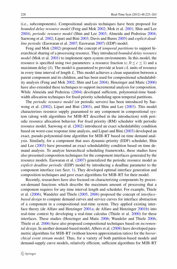
236 Real-Time Syst (2012) 48:223–263

Fig. 4 Space of feasible choicesfor Θ according to Corollary 2.The above scenario representsthe feasibility space whenθ0(1) < θ1(1). a′ represents thepoint of intersection for θ0(a)

and θ1(a). a′−1 is the point ofintersection for θ1(a) and θ2(a)

two cases: (1) Θ ≤ Π and (2) Θ > Π . For Case 1, Θ is also in the interval[θmin(a), θmax(a)] by definition of θmax(a); thus, Theorem 2 is also satisfied and τ

is EDF-schedulable upon Γ . Otherwise, if Case 2 is true, then Γ represents a Θ/Π -speed processor, according to the paragraph preceding the corollary, where Θ/Π > 1.By assumption, τ is EDF-schedulable on a unit-capacity processor; thus, it is clearlymust continue to be EDF-schedulable on a Θ/Π -speed processor. �

At this point, we will make a few observations about Corollary 2:

Observation 1 Both θ0(a) and θ2(a) are monotonically increasing in a.

Observation 2 θ1(a) is monotonically decreasing in a.

Observation 3 θ0(a + 1) = θ2(a).

If θ0(1) ≥ θ1(1), then θmin(a) equals θ0(a) for all a ∈ N+. The fact that θ0(a) ismonotonically increasing implies that θ0(1) is the minimum Θ that will satisfy Corol-lary 2 (since θ0(a) < θ2(a) for all a ∈ N+). If θ0(1) < θ1(1), then the minimum valueof Θ can be achieved when θ0(a

′) = θ1(a′) for some a′ ≥ 1 (i.e., the intersection

of θ0(a) and θ1(a)). This last observation follows from the fact that θ0 is mono-tonically increasing and θ1 is monotonically decreasing. We may determine a′ asfollows.

θ0(a′) = θ1(a

′)

⇒ (a′ + 1)Π − pmin(τ )

1 + a′a′+2

= Π · (a′ + 2)U(τ)

a′ + 2U(τ)

⇒ (a′ + 2)(a′ + 1)Π − (a′ + 2)pmin(τ )

2(a′ + 1)= Π · (a′ + 2)U(τ)

a′ + 2U(τ)

⇒ (

(a′ + 2U(τ))

(a′ + 1)Π − (a′ + 2U(τ))pmin(τ )

− 2(a′ + 1)ΠU(τ) = 0

Real-Time Syst (2012) 48:223–263 237

SUFFICIENTCAPACITY(Π, τ)

1 if θ0(1) ≥ θ1(1)

2 Θ ← θ0(1)

3 else4 Set a′ according to (12).5 if θmin(�a′�) > θ2(�a′�)6 Θ ← θmin(�a′�)7 else8 Θ ← min{θmin(�a′�), θmin(�a′�)}9 return Θ

Fig. 5 Pseudo-code for determining minimum Θ

⇒ Π(a′)2 + [Π + 2ΠU(τ) − pmin(τ ) − 2ΠU(τ)] · a′

− [2ΠU(τ) + 2U(τ)pmin(τ ) − 2ΠU(τ)]= 0

⇒ Π(a′)2 + [Π − pmin(τ )] · a′ − 2U(τ)pmin(τ ) = 0.

The solution a′ may be determined using standard techniques for solving quadraticequations.

a′ = − (Π − pmin(τ )) +√(Π − pmin(τ ))2 + 8ΠU(τ)pmin(τ )

2Π. (12)

In general, a′ as defined above may not be an integer. Therefore, to determine theminimum θmin(a), we should take the minimum of θmin(�a′�) and θmin(�a′�), if[θmin(�a′�), θ2(�a′�)] is non-empty. Otherwise, θmin(�a′�) is the minimum value ofθmin(a) that satisfies Corollary 2, since [θmin(�a′�), θ2(�a′�)] is guaranteed to be non-empty. The pseudocode for determining the minimum Θ that satisfies Corollary 2 isgiven in SUFFICIENTCAPACITY in Fig. 5.

Shin and Lee (2008) show that Theorem 2 (and by extension Corollary 2) performswell in identifying “near-minimum” real-time interfaces over randomly generatedtask systems. However, it is not shown whether any Θ returned from Theorem 2(Corollary 2) can be bounded by a constant approximation ratio from the minimumcapacity Θ∗. We will now show (in the context of permitting over-capacity periodicresources) that Corollary 2 has an approximation ratio of at most three. We first provesome properties of Θ∗.

Lemma 3 Given any implicit-deadline sporadic task system τ and Π ∈ R+, let Θ∗be the minimum capacity such that τ is EDF-schedulable upon periodic resourceΓ ∗ = (Π,Θ∗). If Θ∗ ≤ Π , then

Θ∗ ≥ Π · U(τ). (13)

Proof The proof is by contradiction. Assume that Θ∗ < Π ·U(τ). Thus, U(τ) > Θ∗Π

.By the second condition of Theorem 1 (note that the conditions are same for both EDP

238 Real-Time Syst (2012) 48:223–263

resource Ω and periodic resource Γ ), τ is not EDF-schedulable upon Γ ∗ = (Π,Θ∗).However, this contradicts our supposition that τ is EDF-schedulable on Γ ∗. Thus, ouroriginal assumption is false, and the lemma follows. �

Lemma 4 Given any implicit-deadline sporadic task system τ and Π ∈ R+, let Θ∗be the minimum capacity such that τ is EDF-schedulable upon periodic resourceΓ ∗ = (Π,Θ∗). If Θ∗ ≤ Π , then

Θ∗ ≥ 2Π − pmin(τ ) + δ

2(14)

where δ denotes DBF(τ,pmin(τ )).

Proof We begin by making an observation concerning the optimal value Θ∗. Sinceτ is an implicit-deadline sporadic task system, pmin(τ ) corresponds to the first valueof t such that DBF(τ, t) is positive; thus, δ is positive. Since τ is EDF-schedulableon Γ ∗, DBF(τ, t) ≤ sbf(Γ ∗, t) for all t ≥ 0, it must be that δ ≤ sbf(Γ ∗,pmin(τ )).By definition of sbf (see (8)) and from the assumption that Θ∗ ≤ Π , the previousstatement implies that there must exist some q ∈ N+ such that δ ≤ pmin(τ ) − (q +1)(Π − Θ∗). Solving the preceding inequality for Θ∗, we have

Θ∗ ≥ (q + 1)Π − pmin(τ ) + δ

q + 1. (15)

Since Θ∗ ≤ Π , δ must not exceed pmin(τ ); otherwise, τ would not be schedulableeven on a dedicated processor of unit-speed. The fact that δ − pmin(τ ) ≤ 0 impliesthat the right-hand side of inequality (15) is increasing in q . The lemma follows byobserving the right-hand side is minimized when q equals one. �

We next show that the value returned from SUFFICIENTCAPACITY does not ex-ceed θmin(1).

Lemma 5

min {θmin(a)|(a ∈ N+) ∧ ([θmin(a), θ2(a)] �= ∅)} ≤ θmin(1). (16)

Proof Let X denote the left-hand side of inequality (16). We consider two possiblecases. In each case, we show that X is less θmin(1).

Case I θ0(1) ≥ θ1(1);

or

Case II θ0(1) < θ1(1).

For Case I, Observations 1 and 2 imply that θmin(a) equals θ0(a) for all a ∈ N+. Sinceθ0(a) is monotonically increasing (Observation 1), θmin(1) ≤ θmin(a) for all a ∈ N+.It is easy to see that θ0(a) is strictly less than θ2(a) for all a; thus, [θmin(a), θ2(a)] is

Real-Time Syst (2012) 48:223–263 239

non-empty. Since θ0(1) represents a valid choice of Θ and is the minimum value ofθmin(a) for all a, X is equal to θ0(1) (which equals θmin(1)). Thus, the lemma followsin this case.

For Case II, the argument directly following the statement of Corollary 2 showedthat either θmin(�a′�) or θmin(�a′�) correspond to the value of X. We will considertwo subcases for Case II based on θmin(a) at �a′�:

SubCase II.A The interval [θmin(�a′�), θ2(�a′�)] is non-empty;

or

SubCase II.B [θmin(�a′�), θ2(�a′�)] is empty.

For Subcase II.A, observe that both θmin(�a′�) or θmin(�a′�) are feasible choicesfor X, since θ2(a) exceeds or equals θ0(a) at both �a′� and �a′�. Since �a′� pre-cedes (or equals) the intersection of θ0(a) and θ1(a) and θ0(1) < θ1(1), it mustbe that θ0(a) ≤ θ1(a) for all 1 ≤ a ≤ �a′�. Thus, θ1(a) equals θmin(a) for all1 ≤ a ≤ �a′�. Furthermore, since θ1(a) is monotonically decreasing (Observa-tion 2), θ1(1) ≥ θmin(�a′�). Because X ∈ {θmin(�a′�), θmin(�a′�)} and θmin(�a′�) ≥min{θmin(�a′�), θmin(�a′�)}, it must be that θmin(1) = θ1(1) ≥ X; thus, the lemmafollows in this subcase.

For Subcase II.B, X must be equal to θmin(�a′�). Since θ0(a) is a monotonicallyincreasing function (Observation 1) and �a′� is after the intersection of θ0(a) andθ1(a), it must be that θ0(�a′�) equals θmin(�a′�). To prove the lemma in this case,we must show that θ1(1) is at least θmin(�a′�) (which corresponds to X). To showthis, consider the point at which θ1(a) = θ2(a); denote this point of intersection bya′−1. Since θ1(a) is decreasing in a, it must be that θ1(1) ≥ θ1(a

′−1). By Observa-tion 3, θ0(a

′−1 + 1) equals θ2(a′−1) (which also equals θ1(a

′−1)). Thus, for all a suchthat a′−1 ≤ a ≤ a′−1 + 1, θmin(a) ≤ θ1(a

′−1). See Fig. 4 for a visual explanation. Fur-thermore, it must be that �a′� does not exceed a′−1 + 1 (otherwise, �a′� ≥ a′−1 and[θmin(�a′�), θ2(�a′�)] would be non-empty). Therefore, θmin(�a′�) ≤ θmin(a

′−1); thelemma follows. �

In the next two lemmas, we obtain bounds on θ0(1) and θ1(1) in terms of Θ∗.

Lemma 6 θ0(1) ≤ 32Θ∗.

Proof Consider the ratio θ0(1)Θ∗ where Θ∗ is the optimal minimum capacity given Π

and task system τ . From Lemma 4,

θ0(1)

Θ∗ ≤ θ0(1)

2Π−pmin(τ )+δ2

=3(2Π−pmin(τ ))

42Π−pmin(τ )+δ

2

= 3(2Π − pmin(τ ))

2(2Π − pmin(τ ) + δ)

≤ 3

2.

240 Real-Time Syst (2012) 48:223–263

The last inequality follows from the fact that δ is positive by definition and the preced-ing implication decreases in δ. Since limδ→0 2Π −pmin(τ )+ δ equals 2Π −pmin(τ ),the inequality θ0(1)

Θ∗ ≤ 32 follows. �

Lemma 7 θ1(1) ≤ 3Θ∗.

Proof Consider the ratio θ1(1)Θ∗ . From Lemma 3,

θ1(1)

Θ∗ ≤ θ0(1)

Π · U(τ)= Π · 3U(τ)

1+2U(τ)

Π · U(τ)

= 3

1 + 2U(τ)≤ 3.

The last inequality follows from the fact that preceding expression decreases withU(τ) and U(τ) must be positive. Since limU(τ)→0 1 + 2U(τ) equals one, the in-equality θ0(1)

Θ∗ ≤ 3 follows. �

Theorem 3 (below) follows directly from Lemmas 5, 6, and 7.

Theorem 3 Given any implicit-deadline sporadic task system τ and Π ∈ R+, let Θ

be the minimum value obtained from SUFFICIENTCAPACITY. Let Θ∗ be the minimumcapacity such that τ is EDF-schedulable upon periodic resource Γ ∗ = (Π,Θ∗) withΘ∗ ≤ Π . The following condition regarding Θ and Θ∗ must hold:

Θ∗ ≤ Θ ≤ 3Θ∗. (17)

The above theorem implies that the approximation ratio of SUFFICIENTCAPACITY

is at most three. We may also show a lower bound of 3/2 on the approximation ratioin the theorem below. A “tight” approximation ratio for the application of Theorem 2or Corollary 2 remains open.

Theorem 4 There exists an implicit-deadline sporadic task system τ and Π ∈ R+such that Θ approaches 3

2Θ∗.

Proof Consider an implicit-deadline sporadic task system comprised of a single task:

τdef= {τ1 = (e1, d1,p1) = (δ, γ,∞)} where γ ∈ R+ and 0 < δ <

γ2 . Furthermore, let

Π = γ . We now show that for any such τ and Π the minimum Θ∗ such that τ isEDF-schedulable upon Γ ∗ = (Π,Θ∗) has

Θ∗ = 2Π − γ + δ

2= γ + δ

2. (18)

From the definition of sbf (Definition 2), consider the value of q given Π , Θ∗, and

t ; denote this value by the function q(Π,Θ∗, t) def= max(1, � t−(Π−Θ∗)Π

�). For t = γ ,

we have q(Π,Θ,γ ) = �Θ∗Π

�, since Π = γ . By assumption that τ is EDF-schedulableon a unit-speed processor, Θ∗ ≤ Π . Thus, q(Π,Θ∗, γ ) = 1. By definition of sbf

Real-Time Syst (2012) 48:223–263 241

and the schedulability condition of Theorem 1, if γ ∈ [2Π − 2Θ∗,2Π − Θ∗], thenDBF(τ, γ ) = δ ≤ sbf((Π,Θ∗), γ ) = γ −2Π +2Θ∗. Since p1 equals ∞, there is onlyone step in the DBF(τ, t) function. Thus, DBF(τ, γ ) = sbf((Π,Θ∗), γ ) when Θ∗ isminimized. This case implies (18). If γ �∈ [2Π − 2Θ∗,2Π − Θ∗], then δ ≤ 0 whichis not possible due to our assumption that 0 < δ.

By our choice of γ , δ, and Π , we now show that θ0(1) > θ1(1). Observe that θ0(1)

equals 3γ4 and that θ1(1) equals 3δγ

γ+2δ. By assumption 2δ < γ , which implies that

θ1(1) <3δγ

2δ+2δ= θ0(1). Therefore, SUFFICIENTCAPACITY will return θ0(1) = 3γ

4 .Thus,

Θ

Θ∗ = θ0(1)

Θ∗

= 3γ

2(γ + δ).

Observe limδ→03(γ )

2(γ+δ)equals 3/2. Thus, there exist choices of τ and Π such that Θ

approaches 32Θ∗. �

From Theorem 3 and 4 above, we have shown that the capacity Θ from the suffi-cient algorithm has an approximation ratio in the range 3

2 to 3. In the next section, wegive our algorithm for determining minimum capacity Θ of an EDP resource withina user specified approximation ratio.

5 An algorithm for determining minimum capacity

In Fig. 6, we give pseudocode for our algorithm, MINIMUMCAPACITY, for deter-mining the minimum capacity required to correctly schedule task system τ accordingto EDF upon an EDP resource with given Π and Δ parameters. One of the input pa-rameters is k ∈ N+. If k is some fixed value, then MINIMUMCAPACITY returns anapproximate value for the minimum capacity (as explained in Sect. 6); however, if theinput value of k is equal to ∞, then the returned value will be the actual minimumcapacity.

The intuition behind algorithm MINIMUMCAPACITY is as follows: for eachvalue t in the testing set ˜TS(τ, k) find the minimum capacity Θmin

t requiredto guarantee that the half-line 〈(t, ˜DBF(τ, t, k)),ψ(τ, t, k)〉 is completely beneathsbf((Π,Θmin

t ,Δ), t). By Lemma 2, this half-line is equal to ˜DBF(τ, t, k) until thenext testing set time-point. So, any capacity greater than this minimum capacityΘmin

t will ensure that ˜DBF falls below sbf up until the next point in the testing set.If we set Θ to be the maximum of all these Θmin

t (Line 9 of MINIMUMCAPAC-ITY) and U(τ) · Π , then we ensure that each “step” of ˜DBF(τ, t, k) is strictly lessthan sbf((Π, Θ,Δ), t) and U(τ) ≤ Θ

Π. Since ˜DBF(τ, t, k) ≥ DBF(τ, t) for all t , this

implies that the schedulability condition of Theorem 1 is satisfied; thus, τ is EDF-schedulable upon EDP resource Ω = (Π, Θ,Δ). (Note that if the algorithm returnsΘ > Δ, we cannot guarantee that τ is schedulable upon any EDP resource withparameters Π and Δ executing upon a unit-speed processor.)

242 Real-Time Syst (2012) 48:223–263

MINIMUMCAPACITY(Π,Δ, τ, k)

1 Θ ← U(τ) · Π2 for each t ∈˜TS(τ, k)� (In order)

� For testing set with P(τ) defined as in Theorem 1.3 Dt ← ˜DBF(τ, t, k)

4 α ← ψ(τ, t, k)

5 Θmint ← ∞

6 for � ← max{

1,⌊

t−ΔΠ

⌋}

to(⌈

t+ΔΠ

⌉− 1)

7 Θmin� ← max

⎧

⎪

⎪

⎨

⎪

⎪

⎩

αΠ,Dt−t+�Π+Δ

�+1 ,Dt

�,

Dt+α((�+1)Π+Δ−t)�+2α

⎫

⎪

⎪

⎬

⎪

⎪

⎭

8 Θmint ← min{Θmin

t ,Θmin� }

9 end (of inner loop)10 Θ ← max{Θ,Θmin

t }11 end (of outer loop)12 return Θ

Fig. 6 Pseudo-code for determining minimum capacity for a periodic resource given Π , Δ, and τ . Notethe algorithm is exact when k equals ∞

Algorithm complexity The complexity of MINIMUMCAPACITY depends almost en-tirely upon the cardinality of ˜TS(τ, k). To see this, observe that the inner loop(Lines 6 to 8) has a constant number of iterations due to the fact that 0 ≤ (� t+Δ

Π� −

1) − � t−ΔΠ

� ≤ 2 (since 0 ≤ Δ ≤ Π ). The work inside the inner loop takes constanttime as well. For the outer loop (Lines 2 to 11), the algorithm iterates (in non-decreasing order) through the testing set˜TS(τ, k). Using a “heap-of-heaps” describedby Mok (1988), the time complexity to obtain an element of the testing set is O(lgn).Since for each element of the testing set, t ≡ di + api for some τi ∈ τ and a ∈ N, set-ting Dt and α (Lines 3 and 4) may be done in constant time on each iteration ofthe outer loop. (Dt is increased by ei from prior iteration and α is only increasedby ui , if a = (k − 1).) Therefore, the runtime complexity of MINIMUMCAPACITY

is O(|˜TS(τ, k)| · lgn). If k = ∞, then |˜TS(τ,∞)| ≤ P(τ) which is potentially expo-nential in the number of tasks. The complexity for exactly determining the minimumcapacity is, thus, the same complexity as the test of Theorem 1 on a fixed Ω . Other-wise, if k is a fixed integer, |˜TS(τ, k)| ≤ kn and the complexity is O(kn lgn).

Algorithm correctness To prove the correctness of MINIMUMCAPACITY, we willshow the following theorem which states that the value returned by the algorithm(i.e., Θ) is at least the optimal minimum capacity value Θ∗(Π,Δ, τ). Furthermore,if the input k equals ∞, then the returned capacity is optimal.

Theorem 5 For all k ∈ N+ ∪ {∞}, MINIMUMCAPACITY returns Θ ≥ Θ∗(Π,Δ, τ).Furthermore, if k = ∞, Θ = Θ∗(Π,Δ, τ).

Real-Time Syst (2012) 48:223–263 243

Fig. 7 The solid line “step”function is sbf for Ω . Thedashed line is the lowersupply-bound function lsbf. Theshaded region represents the�-Feasibility Region for � = 2with element 〈(t,Dt ),α〉

In order to prove the above theorem, we require some additional definitions. Thenext definition quantifies the minimum capacity Θ(≤ Δ) that is required for sbf toupper-bound a half-line 〈(t,Dt ),α〉. Definition 4 and 6 uses the function infimum(inf) instead of minimum (min). We will use the convention that inf returns ∞ on anempty set.

Definition 4 (Minimum capacity for 〈(t,Dt ),α〉)Θ∗(Π,Δ, 〈(t,Dt ),α〉)def= inf

{

Θ ∈ R+∣

∣

∣

∣

(Θ ≤ Δ)

∧ (∀x ≥ t : α(x − t) + Dt ≤ sbf((Π,Θ,Δ), t))

}

. (19)

Since sbf is not a continuous function, it is difficult to calculate Θ∗(Π,Δ,

〈(t,Dt ),α〉) in a straightforward linear way. Instead, we break the region below thesbf function into overlapping subregions we call �-feasibility regions for any givenΩ = (Π,Θ,Δ). An �-feasibility region is the area below the �th “step” of the sbffunction extending downward and infinitely to the right. Figure 7 gives a visual de-piction; the definition below formalizes the �-feasibility region concept.

Definition 5 (�-Feasibility region of Ω)

F�(Π,Θ,Δ)def=

⎧

⎪

⎪

⎪

⎨

⎪

⎪

⎪

⎩

〈(t,Dt ),α〉 ∈ R2≥0 × R≥0

∣

∣

∣

∣

∣

∣

∣

∣

∣

(0 ≤ α ≤ ΘΠ

)

∧ (Θ ≥ Dt−t+�Π+Δ�+1 )

∧ (Θ ≥ Dt

�)

∧ (Θ ≥ Dt+α((�+1)Π+Δ−t)�+2α

)

⎫

⎪

⎪

⎪

⎬

⎪

⎪

⎪

⎭

. (20)

The next defined function determines the minimum capacity for any given half-line 〈(t,Dt ),α〉 to be an element of the �-feasibility region.

Definition 6 (�-Minimum capacity for 〈(t,Dt ),α〉)

Θ∗� (Π,Δ, 〈(t,Dt ),α〉) def= inf {Θ(≤ Δ) ∈ R+ | 〈(t,Dt ),α〉 ∈ F�(Π,Θ,Δ)} . (21)

244 Real-Time Syst (2012) 48:223–263

Fig. 8 Illustration of Lemma 8. (a) Originating point of half-line 〈(t,Dt ),α〉 is below lsbf. (b) Originatingpoint of 〈(t,Dt ),α〉 is above lsbf

We begin by showing that the half-line 〈(t,Dt ),α〉 is completely below sbf if andonly if 〈(t,Dt ),α〉 is contained in some �-feasibility region with � > 0.

Lemma 8 For any 〈(t,Dt ),α〉 ∈ R2≥0 × R≥0, α(t ′ − t) + Dt ≤ sbf((Π,Θ,Δ), t ′)

∀t ′ ≥ t if and only if there exists � ∈ N+ such that 〈(t,Dt ),α〉 ∈ F�(Π,Δ,Θ).

Proof We will give a geometric-based proof for this lemma. We will first showthe “if” direction. Assume that 〈(t,Dt ),α〉 ∈ F�(Π,Δ,Θ) for some � ∈ N+. Wemust show that the half-line 〈(t,Dt ),α〉 is completely contained below the sbffunction for Ω = (Π,Θ,Δ). (This is equivalent to showing α(t ′ − t) + Dt ≤sbf((Π,Θ,Δ), t ′) ∀t ′ ≥ t .)

If Dt ≤ lsbf((Π,Θ,Δ), t), then the half-line 〈(t,Dt ),α〉 is below lsbf(Ω, t ′) forall t ′ ≥ t , because the slope of the half-line (i.e., α) is at most Θ

Πthat is, the slope

of lsbf(Ω, t) (see Fig. 8a). α ≤ ΘΠ

follows from (20). Since lsbf(Ω, t ′) ≤ sbf(Ω, t ′)for all t ′ ≥ t , this implies that the half-line 〈(t,Dt ),α〉 never exceeds lsbf for Ω =(Π,Θ,Δ). Otherwise, if Dt > lsbf((Π,Θ,Δ), t), the originating point of the half-line 〈(t,Dt ),α〉 is contained within the triangular convex region defined by the (x, y)-points (�Π +Δ−2Θ,(�−1)Θ), (�Π +Δ−Θ,�Θ), and ((�+1)Π +Δ−2Θ,�Θ);this region is formed by the intersection of the half-plane y > lsbf((Π,Θ,Δ), x)

and the �-feasibility region; e.g., see Fig. 8b. From the figure it is obvious that thistriangular region is contained below sbf. Furthermore, the entire �-feasibility regionis contained below sbf; thus, Dt ≤ sbf((Π,Θ,Δ), t). If we can show that the half-line 〈(t,Dt ),α〉’s value is below �Θ at t1 = (� + 1)Π + Δ − 2Θ , then [t, t1] intervalportion of the half-line is contained entirely within the �-feasibility region (and, thus,below sbf), and the remaining [t1,∞) portion of the half-line falls below lsbf (and,thus, sbf). From the fourth condition of (20), it must be that �Θ ≥ Dt +α((�+1)Π +Δ − 2Θ − t) which is equivalent to 〈(t,Dt ),α〉 being less than �Θ at t1. Thus, ineither case (based on the relative values of Dt and lsbf(Ω, t)), we show the half-line〈(t,Dt ),α〉 must be completely contained below the sbf function for Ω .

For the “only if” direction, we must show that if the half-line 〈(t,Dt ),α〉 is com-pletely contained below the sbf function for Ω , then there exists an � ∈ N+ suchthat 〈(t,Dt ),α〉 ∈ F�(Π,Θ,Δ). Consider � = �Dt

Θ�. (If Θ = 0, then we will sim-

ply use � = 0, since in this case Dt must be zero due to sbf((Π,0,Δ), t) = 0 for

Real-Time Syst (2012) 48:223–263 245

all t > 0.) The third condition of (20) is trivially satisfied for this �. It also mustbe true that Dt > (� − 1)Θ . Thus, (t,Dt ) must be below of the line defined byy = x − (�Π + Δ − (� + 1)Θ) (otherwise, (t,Dt ) would be above the sbf functionat t). This last constraint is equivalent to the second condition of (20). The half-line’sslope α obviously must not exceed Θ

Π; otherwise, the 〈(t,Dt ),α〉 would eventually

exceed sbf at some point. This constraint corresponds to the first condition of (20).Finally, �Θ must be greater than the value of 〈(t,Dt ),α〉 at t1 = (�+1)Π +Δ−2Θ ;otherwise, the half-line would exceed sbf at t1. By the previous paragraph, weshowed that this condition corresponds to satisfying the fourth condition of (20).Therefore, for � = �Dt

Θ� we have satisfied all four conditions of (20), implying that

〈(t,Dt ),α〉 ∈ F� DtΘ

�(Π,Θ,Δ). �

Lemma 9 For any � ∈ N+,

Θ∗� (Π,Δ, 〈(t,Dt ),α〉) = max

⎧

⎪

⎪

⎨

⎪

⎪

⎩

αΠ,Dt−t+�Π+Δ

�+1 ,Dt

�,

Dt+α((�+1)Π+Δ−t)�+2α

⎫

⎪

⎪

⎬

⎪

⎪

⎭

. (22)

Proof Let ΘRHS denote the right-hand side of (22). We will show that both ΘRHS ≥Θ∗

� (Π,Δ, 〈(t,Dt ),α〉) and ΘRHS ≤ Θ∗� (Π,Δ, 〈(t,Dt ),α〉) which will imply the

lemma. The inequality ΘRHS ≥ Θ∗� (Π,Δ, 〈(t,Dt ),α〉) follows from the observation

that 〈(t,Dt ),α〉 ∈ F�(Π,ΘRHS,Δ) (i.e., the four conditions of (20) imply the lowerbound).

We will show ΘRHS ≤ Θ∗� (Π,Δ, 〈(t,Dt ),α〉) by contradiction. Assume the nega-

tion of the inequality. In this case, since ΘRHS > Θ∗� (Π,Δ, 〈(t,Dt ),α〉), it must be

that Θ∗� (Π,Δ, 〈(t,Dt ),α〉) is strictly less than at least one of the four terms in the

RHS of (22); however, this implies that 〈(t,Dt ),α〉 �∈ F�(Π,Θ∗� (Π,Δ, 〈(t,Dt ),α〉),

Δ). The previous statement contradicts Definition 6; thus, it must be that ΘRHS ≤Θ∗

� (Π,Δ, 〈(t,Dt ),α〉) is true. �

Now that we know how to efficiently compute Θ∗� (Π,Δ, 〈(t,Dt ),α〉) by simply

checking the four values defined by the previous lemma, it would be convenient touse this value to compute the overall minimum capacity for half-line 〈(t,Dt ),α〉. Thenext lemma shows that this minimum bandwidth can be found by taking the minimum�-minimum capacity for all positive �.

Lemma 10

Θ∗(Π,Δ, 〈(t,Dt ),α〉) = inf�>0

{

Θ∗� (Π,Δ, 〈(t,Dt ),α〉)} . (23)

Proof Let ΘRHS denote the right-hand side of (23). We will show that both ΘRHS ≥Θ∗(Π,Δ, 〈(t,Dt ),α〉) and ΘRHS ≤ Θ∗(Π,Δ, 〈(t,Dt ),α〉) which will imply thelemma. First, we show ΘRHS ≥ Θ∗(Π,Δ, 〈(t,Dt ),α〉). By definition of infimum,for any δ > 0, there exists � ∈ N+ such that {Θ∗

� (Π,Δ, 〈(t,Dt ),α〉)} ≤ ΘRHS + δ.Definition 6 states that 〈(t,Dt ),α〉 ∈ F�(Π,ΘRHS + δ,Δ) for this �. Lemma 8 then

246 Real-Time Syst (2012) 48:223–263

implies that α(t ′ − t) + Dt ≤ sbf((Π,ΘRHS + δ,Δ), t ′) for all t ′ ≥ t . Therefore, forall δ > 0, ΘRHS + δ must be in the set considered in the inf on the right-hand sideof (19) in Definition 4. Thus, ΘRHS ≥ Θ∗(Π,Δ, 〈(t,Dt ),α〉).

Next, we will show ΘRHS ≤ Θ∗(Π,Δ, 〈(t,Dt ),α〉). By Definition 4,

∀x ≥ t : α · (x − t) + Dt ≤ sbf((Π,Δ,Θ∗(Π,Δ, 〈(t,Dt ),α〉)), t).Lemma 8 implies that there exists � ∈ N+ such that 〈(t,Dt ),α〉 ∈ F�(Π,Θ∗(Π,Δ,

〈(t,Dt ),α〉),Δ). By Definition 6, this implies that Θ∗(Π,Δ, 〈(t,Dt ),α〉) is in theset considered in the right-hand side of (21) which implies the inequality. �

Fortunately, we do not need to evaluate Θ∗� (Π,Δ, 〈(t,Dt ),α〉) for all positive

� to compute the minimum capacity for half-line 〈(t,Dt ),α〉. In the next lemmaand corollary, we show that the smallest value of � that needs to be considered ismax(1, � t−Δ

Π�) for a given Π and Δ. For all values of �′ smaller than this value, we

can show that Θ∗�′(Π,Δ, 〈(t,Dt ),α〉) ≥ Θ∗

max(1,� t−ΔΠ

�)(Π,Δ, 〈(t,Dt ),α〉).

Lemma 11 For any �, �′ ∈ N+ and Dt, t, α ∈ R≥0, if (t ≥ �Π + Δ), (�′ < �), and(α ≤ 1), then

[〈(t,Dt ),α〉 ∈ F�′(Π,Θ,Δ)] ⇒ [〈(t,Dt ),α〉 ∈ F�(Π,Θ,Δ)] . (24)

Proof Assume that 〈(t,Dt ),α〉 ∈ F�′(Π,Θ,Δ). We must show that all four condi-tions of (20) are satisfied for F�. First note that 〈(t,Dt ),α〉 ∈ F�′(Π,Θ,Δ) impliesthat α ≤ Θ

Π; thus, the first condition of (5) is trivially satisfied for F�. By the third

condition of (20) for F�′ , Dt ≤ �′Θ . Since � > �′, it must also be that Dt ≤ �Θ

(which satisfies third condition for F�). Similarly, the fourth condition of (20) for F�′implies that �′Θ ≥ α((�′ + 1)Π + Δ − 2Θ − t) + Dt . Since Θ ≥ αΠ and � ≥ �′, thefourth condition for F� is also satisfied. Finally, consider the following expression

t − �Π − Δ + (� + 1)Θ

≥ (�Π + Δ) − (�Π + Δ) + (� + 1)Θ (by assumption on t)

= (� + 1)Θ

> �′Θ

≥ Dt (from condition three for F�′).

The above derivation implies the second condition for F� which proves the lemma. �

Given t , Π , and Δ, consider � = max(1, � t−ΔΠ

�). For any Dt , α, and �′ < � whichsatisfy the supposition of the above lemma, it must be that.

{Θ(≤ Δ) ∈ R+ | 〈(t,Dt ),α〉 ∈ F�′(Π,Θ,Δ)}⊆{

Θ(≤ Δ) ∈ R+ | 〈(t,Dt ),α〉 ∈ Fmax(1,� t−ΔΠ

�)(Π,Θ,Δ)}

.

By the above expression and (21) of Definition 6, the corollary below follows imme-diately.

Real-Time Syst (2012) 48:223–263 247

Corollary 3 For any �′ ∈ N+ and Dt, t, α ∈ R≥0, if (�′ < max(1, � t−ΔΠ

�)) and (α ≤1), then

Θ∗�′(Π,Δ, 〈(t,Dt ),α〉) ≥ Θ∗

max(1,� t−ΔΠ

�)(Π,Δ, 〈(t,Dt ),α〉).

In the following two lemmas and one corollary, we show that the largest valueof � that needs to be considered is � t+Δ

Π� − 1 for a given Π and Δ. For all

values of �′ larger than this value, we can show that Θ∗�′(Π,Δ, 〈(t,Dt ),α〉) ≥

Θ∗� t+Δ

Π�−1

(Π,Δ, 〈(t,Dt ),α〉).

Lemma 12 For any �, �′ ∈ N+ and Dt, t, α ∈ R≥0, if (t ≤ �Π − Δ), (�′ ≥ � − 1),and (α ≤ 1), then

[〈(t,Dt ),α〉 �∈ F�′(Π,Θ,Δ)]⇒ [〈(t,Dt ),α〉 �∈ F�′+1(Π,Θ,Δ)

]

.

Proof Assume that 〈(t,Dt ),α〉 �∈ F�′(Π,Θ,Δ). This implies that at least one of thefollowing is true:

α >Θ

Π(25a)

Θ <Dt − t + �′Π + Δ

�′ + 1(25b)

Θ <Dt

�′ (25c)

Θ <Dt + α((�′ + 1)Π + Δ − t)

�′ + 2α. (25d)

We will show that each of the above inequalities implies that 〈(t,Dt ),α〉 �∈F�′+1(Π,Θ,Δ). Obviously, (25a) trivially implies the aforementioned expression.If (25b) is true, then

Dt > t − �′Π − Δ + (�′ + 1)Θ

⇒ Dt > t − (�′ + 1)Π − Δ + (�′ + 2)Θ

⇒ Θ >Dt − t + (�′ + 1)Π + Δ

�′ + 2.

The first implication above is due to the fact that right-hand side of the first inequalityin the derivation is non-increasing in �′ (since Θ ≤ Π ). Thus, if (25b) is true, then〈(t,Dt ),α〉 �∈ F�′+1(Π,Θ,Δ).

If (25c) is true, then consider the following expression:

t − (�′ + 1)Π − Δ + (�′ + 2)Θ

≤ �Π − Δ − (�′ + 1)Π − Δ + (�′ + 2)Θ

248 Real-Time Syst (2012) 48:223–263

(by supposition on t)

≤ �Π − �Π − 2Δ + (�′ + 2)Θ (by �′ ≥ � − 1)

≤ (�′ + 2)Θ − 2Θ (by Δ ≥ Θ)

= �′Θ

< Dt (by (25c)).

Thus, Θ <Dt−t+(�′+1)Π+Δ

�′+2 which implies 〈(t,Dt ),α〉 �∈ F�′+1(Π,Θ,Δ).Finally, if (25d) is true, then

�′Θ < Dt + α((�′ + 1)Π + Δ − 2Θ − t)

⇒ �′Θ < Dt + (�′ + 1)Π + Δ − 2Θ − t

⇒ (�′ + 2)Θ < Dt + (�′ + 1)Π + Δ − t

⇒ Θ <Dt − t + (�′ + 1)Π + Δ

�′ + 2.

The first implication is due to α ≤ 1. The last inequality implies that when (25d) istrue, 〈(t,Dt ),α〉 �∈ F�′+1(Π,Θ,Δ); the lemma follows. �

Lemma 13 For any �, �′ ∈ N+ and Dt, t, α ∈ R≥0, if (t ≤ �Π − Δ), (�′ > � − 1),and (α ≤ 1), then

[〈(t,Dt ),α〉 ∈ F�′(Π,Θ,Δ)] ⇒ [〈(t,Dt ),α〉 ∈ F�−1(Π,Θ,Δ)]

.

Proof By the contrapositive of Lemma 12, if 〈(t,Dt ),α〉 ∈ F�′(Π,Θ,Δ), then〈(t,Dt ),α〉 ∈ F�′−1(Π,Θ,Δ). If �′ −1 equals �−1, then we have shown the lemma.Otherwise, the lemma follows from repeated application of the contrapositive ofLemma 12. �

Given t , Π , and Δ, consider � = � t+ΔΠ

�. For any Dt,α, �′ > � − 1 which satisfythe supposition of the above lemma, it must be that.

{Θ(≤ Δ) ∈ R+ | 〈(t,Dt ),α〉 ∈ F�′(Π,Θ,Δ)}⊆{

Θ(≤ Δ) ∈ R+ | 〈(t,Dt ),α〉 ∈ F� t+ΔΠ

�−1(Π,Θ,Δ)}

.

By the above expression and (21) of Definition 6, the corollary below follows imme-diately.

Corollary 4 For a given Π , Δ, and 〈(t,Dt ),α〉, the following is true for all �′ >

� t+ΔΠ

� − 1,

Θ∗�′(Π,Δ, 〈(t,Dt ),α〉) ≥ Θ∗

� t+ΔΠ

�−1(Π,Δ, 〈(t,Dt ),α〉).

Real-Time Syst (2012) 48:223–263 249

Combining Corollaries 3 and 4 with Lemma 10, we obtain the following corollarywhich shows that Θ∗(Π,Δ, 〈(t,Dt ),α〉) may be calculated with only a small numberof values for �.

Corollary 5

Θ∗(Π,Δ, 〈(t,Dt ),α〉)

= minmax{1,(� t−Δ

Π�)}

≤ � ≤(⌈

t + Δ

Π

⌉

− 1

)

{

Θ∗� (Π,Δ, 〈(t,Dt ),α〉)} .

The next lemma shows the maximum value of Θ obtained from calculating Θ∗(·)for every value in the testing set ˜TS(τ, k) may be used safely as a capacity which willsatisfy the condition of Theorem 1 (i.e., the EDP schedulability condition).

Lemma 14 For any t ≥ 0, ˜DBF(τ, t, k) ≤ sbf((Π,Θ,Δ), t) and U(τ) ≤ ΘΠ

, if andonly if,

Θ ≥ max

(

maxt∈˜TS(τ,k)

{

Θ∗ (Π,Δ, 〈(t, ˜DBF(τ, t, k)),ψ(τ, t, k)〉)} ,

U(τ) · Π)

. (26)

Proof We will show the “if” direction first, by showing its contrapositive. We mustshow that if either U(τ) > Θ

Πor ∃t ≥ 0 : ˜DBF(τ, t, k) > sbf((Π,Θ,Δ), t), then the

negation of the inequality of (26) is also true. Assume that U(τ) > ΘΠ

. By the secondexpression in the outer “max” of (26), the negation of the inequality is true. Now,assume there exists t ≥ 0 such that ˜DBF(τ, t, k) > sbf((Π,Θ,Δ), t). There must existtwo consecutive values ta and ta+1 in ˜TS(τ, k) where t ∈ [ta, ta+1). (Recall that if tais the largest value in ˜TS(τ, k) then ta+1 is assumed to be ∞.) Lemma 2 implies thatfor all t ′ ∈ [ta, ta+1), ˜DBF(τ, t ′, k) equals ψ(τ, ta, k) · (t ′ − ta) + ˜DBF(τ, ta, k). Sincet ∈ [ta, ta+1),

sbf((Π,Θ,Δ), t) < ψ(τ, ta, k) · (t − ta) + ˜DBF(τ, ta, k).

By Lemma 8, this implies that for all � ∈ N+,

〈(ta, ˜DBF(τ, ta, k)),ψ(τ, ta, k)〉 �∈ F�(Π,Θ,Δ).

By (21) from Definition 6,

Θ < Θ∗� (Π,Δ, 〈(ta, ˜DBF(τ, ta, k)),ψ(τ, ta, k)〉)

for all � ∈ N+, which implies (by Lemma 10)

Θ < Θ∗(Π,Δ, 〈(ta, ˜DBF(τ, ta, k)),ψ(τ, ta, k)〉).Thus, Θ < maxt∈˜TS(τ,k){Θ∗(Π,Δ, 〈(t, ˜DBF(τ, t, k)),ψ(τ, t, k)〉)}. Again, the nega-tion of the inequality of (26) is true. The contrapositive of the “if” direction follows.

For the “only if” direction of the lemma, we will also consider the contrapositive.The contrapositive will follow by simply reversing the implications of the proof for

250 Real-Time Syst (2012) 48:223–263

the “if” direction. We give the argument for completeness. Assume that the negationof the inequality of (26). If Θ < U(τ) · Π , then obviously U(τ) > Θ

Π. Otherwise, if

Θ < maxt∈˜TS(τ,k)

{

Θ∗ (Π,Δ, 〈(t, ˜DBF(τ, t, k)),ψ(τ, t, k)〉)} ,

then there exists ta ∈ ˜TS(τ, k) such that Θ < Θ∗(Π,Δ, 〈(ta, ˜DBF(τ, ta, k)),

ψ(τ, ta, k)〉). By Lemma 10,

Θ < Θ∗� (Π,Δ, 〈(ta, ˜DBF(τ, ta, k)),ψ(τ, ta, k)〉)

for all � ∈ N+. From (21) from Definition 6, 〈(ta, ˜DBF(τ, ta, k)),ψ(τ, ta, k)〉 �∈F�(Π,Θ,Δ) for all � ∈ N+. By Lemma 8, there exists a t ≥ ta such thatsbf((Π,Θ,Δ), t) < ψ(τ, ta, k) · (t − ta) + ˜DBF(τ, ta, k). Lemma 2 implies that forall t ′ ≥ ta , ˜DBF(τ, t ′, k) is at least ψ(τ, ta, k) · (t ′ − ta) + ˜DBF(τ, ta, k). Thus, sincet ≥ ta , sbf((Π,Θ,Δ), t) < ˜DBF(τ, t, k). The contrapositive of the “only if” directionfollows. �

After proving the above lemma, we may now prove Theorem 5 which states thatMINIMUMCAPACITY returns a valid capacity (i.e., τ is schedulable upon the returnedcapacity) for finite k and an exact value for k = ∞.

Proof of Theorem 5 It is easy to see that Θ returned from MINIMUMCAPACITY

corresponds to the value on the right-hand side of (26) of Lemma 14; the loopfrom Line 2 to 11 iterate through each value ta in ˜TS(τ, k) (setting variables cor-responding to ˜DBF(τ, ta, k) and ψ(τ, ta, k) in Lines 3 and 4, respectively). The in-ner loop from Line 6 to 8 determines Θ∗(Π,Δ, 〈(ta, ˜DBF(τ, ta, k)),ψ(τ, ta, k)〉);the implications of Corollary 5 and Lemma 10 show that we need to calculateΘ∗

� (Π,Δ, 〈(ta, ˜DBF(τ, ta, k)),ψ(τ, ta, k)〉) only for values of � from max(1, � ta−ΔΠ

�)to � ta+Δ

Π� − 1. Finally, in Line 9, Θ is set to the maximum of U(τ) · Π and

Θ∗(Π,Δ, 〈(ta, ˜DBF(τ, ta, k)),ψ(τ, ta, k)〉) over all values ta in ˜TS(τ, k).By Lemma 14, ˜DBF(τ, t, k) ≤ sbf((Π, Θ,Δ), t) for all t ≥ 0 and U(τ) ≤ Θ

Π.

By Lemma 1, DBF(τ, t) ≤ ˜DBF(τ, t, k) ≤ sbf((Π, Θ,Δ), t) for all t ≥ 0. Therefore,the suppositions of Theorem 1 are satisfied and τ will always meet all deadlineswhen scheduled by EDF upon Ω = (Π, Θ,Δ). When k = ∞, ˜DBF(τ, t, k) equalsDBF(τ, t) for all t ≥ 0; in this case, Θ equals Θ∗(Π,Δ, τ) (i.e., Θ is an exact value)due to the fact that both Lemma 14 and Theorem 1 are necessary and sufficient. �

6 An approximation scheme

In the previous section, we have shown that MINIMUMCAPACITY gives a valid an-swer when k is finite and an exact answer when k is infinite. When k is finite, we havenot, yet, given any details on how accurate the returned Θ will be. In this section, weshow that we may trade computational efficiency for accuracy; that is, as k increasesthe guaranteed accuracy of MINIMUMCAPACITY increases along with its runningtime. Theorem 6 quantifies this tradeoff for a given k; Corollary 7 shows that this

Real-Time Syst (2012) 48:223–263 251

tradeoff permits an FPTAS for the MIB-RT problem. Before we prove Theorem 6and Corollary 7, we need to prove two technical lemmas.

Lemma 15 Given Π , Δ, and τ , the following is true for all k, �(∈ N+), t,Dt (∈ R+),and α(∈ [0,1]),

Θ∗� (Π,Δ, 〈(t,Dt ),α〉) ≤

(

k + 1

k

)

· Θ∗�

(

Π,Δ,

⟨(

t,k · Dt

k + 1

)

,k · αk + 1

⟩)

. (27)

Proof By Lemma 9, Θ∗� (Π,Δ, 〈(t,Dt ),α〉) must be equal to one of the follow-

ing: αΠ ; Dt−t+�Π+Δ�+1 ; Dt

�; or Dt+α((�+1)Π+Δ−t)

�+2α. We will show that for each of the

four possibilities, (27) must hold. If Θ∗� (Π,Δ, 〈(t,Dt ),α〉) is equal to αΠ , then by

Lemma 9,

Θ∗�

(

Π,Δ,

⟨(

t,k · Dt

k + 1

)

,k · αk + 1

⟩)

≥(

k · αk + 1

)

· Π

=(

k

k + 1

)

· Θ∗� (Π,Δ, 〈(t,Dt ),α〉) .

The last step implies (27).If Θ∗

� (Π,Δ, 〈(t,Dt ),α〉) is equal to Dt−t+�Π+Δ�+1 , we will consider two subcases:

t ≤ �Π + Δ and t > �Π + Δ. If t ≤ �Π + Δ, then by Lemma 9,

Θ∗�

(

Π,Δ,

⟨(

t,k · Dt

k + 1

)

,k · αk + 1

⟩)

≥k·Dt

k+1 − t + �Π + Δ

� + 1

≥(

k

k + 1

)

·(

Dt − t + �Π + Δ

� + 1

)

=(

k

k + 1

)

· Θ∗� (Π,Δ, 〈(t,Dt ),α〉) .

Otherwise, t > �Π + Δ. In this case, Lemma 9 also implies

Θ∗�

(

Π,Δ,

⟨(

t,k · Dt

k + 1

)

,k · αk + 1

⟩)

≥k·Dt

k+1

�

≥ ( kk+1 ) · Dt − ( k

k+1 )(t − �Π + Δ)

� + 1

252 Real-Time Syst (2012) 48:223–263

=(

k

k + 1

)

·(

Dt − t + �Π + Δ

� + 1

)

=(

k

k + 1

)

· Θ∗� (Π,Δ, 〈(t,Dt ),α〉) .

Thus, in either subcase, (27) holds.If Θ∗

� (Π,Δ, 〈(t,Dt ),α〉) is equal to Dt

�, then Lemma 9 implies

Θ∗�

(

Π,Δ,

⟨(

t,k · Dt

k + 1

)

,k · αk + 1

⟩)

≥k·Dt

k+1

�

=(

k

k + 1

)

· Θ∗� (Π,Δ, 〈(t,Dt ),α〉) .

Finally, if Θ∗� (Π,Δ, 〈(t,Dt ),α〉) is equal to Dt+α((�+1)Π+Δ−t)

�+2α, then Lemma 9

implies that

Θ∗�

(

Π,Δ,

⟨(

t,k · Dt

k + 1

)

,k · αk + 1

⟩)

≥k·Dt

k+1 − ( k·αk+1 )((� + 1)Π + Δ − t)

� + 2 · ( k·αk+1 )

≥(

k

k + 1

)

·(

Dt − α ((� + 1)Π + Δ − t)

� + 2α

)

=(

k

k + 1

)

· Θ∗� (Π,Δ, 〈(t,Dt ),α〉) . �

Lemma 16 Given Π , Δ, and τ , the following is true for all k ∈ N+ and ta ∈˜TS(τ, k),

Θ∗(Π,Δ, τ) ≥ Θ∗(

Π,Δ,

⟨(

ta,k · ˜DBF(τ, ta, k)

k + 1

)

,k · ψ(τ, ta, k)

k + 1

⟩)

. (28)

Proof Let ΘRHS denote the right-hand side of (28). By definition of Θ∗(Π,Δ, τ)

and Theorem 1,

sbf((Π,Θ∗(Π,Δ, τ),Δ), t) ≥ DBF(τ, t) : ∀t ≥ 0. (29)

Now consider any ta ∈˜TS(τ, k). By combining Lemma 1 and Lemma 2, we have, forall t ≥ ta ,

(

k + 1

k

)

· DBF(τ, t) ≥ ψ(τ, ta, k) · (t − ta) + ˜DBF(τ, ta, k). (30)

Real-Time Syst (2012) 48:223–263 253

Combining the inequalities of (29) and (30) gives us, for all t ≥ ta ,

sbf((Π,Θ∗(Π,Δ, τ),Δ), t) ≥(

k·ψ(τ,ta,k)k+1

)

· (t − ta) + k·˜DBF(τ,ta,k)k+1 . (31)

Lemma 8 and (31) imply that there exists � ∈ N+ such that

⟨(

ta,k · ˜DBF(τ, ta, k)

k + 1

)

,k · ψ(τ, ta, k)

k + 1

⟩

∈ F�(Π,Θ∗(Π,Δ, τ),Δ). (32)

The above expression and Definition 6 imply

Θ∗�

(

Π,Δ,

⟨(

ta,k · ˜DBF(τ, ta, k)

k + 1

)

,k · ψ(τ, ta, k)

k + 1

⟩)

≤ Θ∗(Π,Δ, τ). (33)

The lemma follows from the expression above and Lemma 10. �

The following corollary gives upper and lower bounds on the value obtained fromthe approximation. The corollary follows by combining Lemmas 15 and 16.

Corollary 6 Given Π , Δ, and τ , the following is true for all k ∈ N+ and t ∈˜TS(τ, k),(

k + 1

k

)

· Θ∗(Π,Δ, τ) ≥ min�∈N+

{

Θ∗�

(

Π,Δ,⟨(

t, ˜DBF(τ, t, k))

,ψ(τ, t, k)⟩)}

. (34)

Finally, we give the theorem which quantifies the tradeoff between accuracy andcomputational complexity, in terms of k.

Theorem 6 Given Π , Δ, τ , and k ∈ N+, the procedure MINIMUMCAPACITY returnsΘ such that

Θ∗(Π,Δ, τ) ≤ Θ ≤(

k + 1

k

)

· Θ∗(Π,Δ, τ).

Furthermore, MINIMUMCAPACITY(Π,Δ, τ, k) has time complexity O(kn lgn)

Proof Theorem 5 shows that Θ∗(Π,Δ, τ) ≤ Θ ; thus, we are left to prove the secondinequality of the theorem. There are two cases that we will consider: Θ = U(τ) · Πand Θ > U(τ) ·Π . (Observe by Line 1, Θ must be at least U(τ) ·Π .) In the case thatΘ equals U(τ) · Π , Theorem 1 implies that Θ∗(Π,Δ, τ) must be at least U(τ) · Π .For this case, the second inequality follows, since k+1

k≥ 1 for all k ∈ N+.

In the case that Θ exceeds U(τ) · Π , Θ must equal

maxt∈˜TS(τ,k)

{

Θ∗ (Π,Δ, 〈(t, ˜DBF(τ, t, k)),ψ(τ, t, k)〉)}

according to the proof of Theorem 5. By Lemma 10, this is equivalent to

maxt∈˜TS(τ,k)

{

min�∈N+

{

Θ∗�

(

Π,Δ, 〈(t, ˜DBF(τ, t, k)),ψ(τ, t, k)〉)}}

.

254 Real-Time Syst (2012) 48:223–263

Applying Corollary 6 immediately yields the second inequality of the theorem forthis case. �

If we are given an accuracy parameter ε > 0, we can appropriately set k equal to� 1

ε� and guarantee an (1+ ε) approximation ratio from the result returned from MIN-

IMUMCAPACITY. The following corollary (which follows from Theorem 6) showsthat this approach yields an FPTAS for MIB-RT.

Corollary 7 Given Π , Δ, τ , and ε > 0, the procedure MINIMUMCAPACITY(Π,Δ,

τ, � 1ε�) returns Θ such that

Θ∗(Π,Δ, τ) ≤ Θ ≤ (1 + ε) · Θ∗(Π,Δ, τ).

Furthermore, MINIMUMCAPACITY(Π,Δ, τ, � 1ε�) has time complexity O(

n lgnε

).

7 Evaluation

In this section, we first give an illustrative example of the effectiveness of our ap-proach over both the exact algorithm and the sufficient algorithm. We then show theeffectiveness in simulations over randomly-generated task systems.

7.1 An example

Consider a component C of a compositional system consisting of three sporadictasks τ1 = (3,15,15), τ2 = (3,8,8) and τ3 = (4,18,18). For the exact schedula-bility test, we need to calculate the lcm of periods, and the testing set TS will consistof {8,15,16,18,24,30, . . . ,378}—a total of 82 unique points. If we approximatethe demand bound function at k = 3, the approximate testing set ˜TS will consistof {8,15,16,18,24,30,36,45,54}—a total of nine points. Thus, approximating dbfreduces complexity to polynomial in number of tasks and k. Now, if we considerΠ = 10 and Δ = Π as the resource to the system, the optimal minimum capacity Θ∗obtained from MINIMUMCAPACITY using k = ∞ is 8.33. Approximate minimumcapacity Θ obtained from MINIMUMCAPACITY using k = 3 is 8.43 and sufficientcapacity Θ from SUFFICIENTCAPACITY is 9.21. From this example, we may ob-serve a very small loss of accuracy (relative error5 1.2%) for MINIMUMCAPACITY

when compared with the optimal and SUFFICIENTCAPACITY (relative error 10.5%).Furthermore, our algorithm achieves a low loss of accuracy with 1/9’th the numberof points as the exact algorithm. In the next subsection, we will show this observationholds over randomly-generated systems, in general.

5Relative error is defined as follows: Θ−Θ∗Θ∗ . In this case, the exact capacity is Θ∗ and the estimated

capacity Θ is either the sufficient capacity Θ or approximate capacity Θ .

Real-Time Syst (2012) 48:223–263 255

7.2 Simulations

In this section, we show the simulation results for our proposed algorithm and com-pare it with the exact (Theorem 1) (Easwaran et al. 2007) and the sufficient algorithm(Theorem 2) (Shin and Lee 2008). During simulations, we have the following simu-lation parameters and value ranges:

1. The number of tasks (n) in the task system τ is taken from the set {2,4,6,8, . . . ,

24}.2. The system utilization U(τ) is taken from the range [0.1,0.8] at 0.05-increments

and individual task utilizations ui are generated using UUniFast algorithm (Biniand Buttazzo 2004). For a specific system utilization U(τ), this algorithm gener-ates n random numbers in the range [0,U(τ)] from uniform distribution in such away that the sum of the numbers equals the system utilization U(τ).

3. Each sporadic task τi = (ei, di,pi) has a period pi uniformly drawn from theinterval [5,40]. (A small period range is used to keep P(τ) from becoming toolarge.) The execution time ei is set to ui × pi . For each task, di = pi .

4. The component level scheduling algorithm is EDF.5. The value of k is taken from the set {1,3,5, . . . ,19}; Π is taken from the set

{5,10,15, . . . ,40}; Δ is set equal to Π .

For each simulation, given task system size n and system utilization U(τ), we ran-domly generate taskset parameters ui,pi , and ei for each task τi . We implementedthe linear time algorithm SUFFICIENTCAPACITY, the exact algorithm (Easwaran etal. 2007; Shin and Lee 2008) and MINIMUMCAPACITY in MATLAB to generate suf-ficient, exact and approximate capacity, respectively. We have used two machines inour simulations with the following specifications: an Intel i-7 950 (four-core CPUwith two hardware threads per core) machine with 6 GB RAM and a Phenom II X61100T (six-core CPU) machine with 8 GB RAM. To exploit the benefit of a multi-core architecture, we have used ‘parfor’ function of MATLAB instead of a regular‘for’ loop. Using this function, the simulation runs are concurrently executed on thecores of the CPU, which allowed us a significant speed-up in the duration of thesimulations.

Our comparison metrics are relative error, testing set size and execution time ofthe algorithms. We compare relative error of our algorithm with the sufficient algo-rithm, and the other two metric of our algorithm with the exact algorithm. For oursimulations, we vary the task system utilization (Figs. 9, 10, and 16), resource period(Figs. 13, 14, and 18), and task system size (Figs. 11, 12, and 17) and evaluated eachof the comparison metrics above. We also varied the approximation parameter k toevaluate the change in relative error (Fig. 15). For the plots which vary the system uti-lization, resource period, or approximation parameter, each point represents the meanvalue of the comparison metric over 1000 simulation runs. For the plots which varytask system size, we reduced the number of simulation runs per point to 300. (Us-ing 1000 runs for this experiment requires the simulation to execute for more thanone week!) The 95% confidence intervals are shown for all the plots.

In Fig. 9, relative error in calculation of capacity for the two algorithms are plottedas a function of task system utilization. In the graph, the dotted-line curve represents

256 Real-Time Syst (2012) 48:223–263

Fig. 9 Relative error vs systemutilization

Fig. 10 Testing set size vssystem utilization

relative error for Θ and the solid-line curve represents relative error for Θ . For MIN-IMUMCAPACITY, the mean relative error is less than 5%, whereas for the sufficientalgorithm it ranges from 15% to 50%. Please note that approximation ratio for Θ

is between 3/2 and 3 as shown in Sect. 4.2 whereas the approximation ratio for Θis at most 4/3 when k = 3 (from Theorem 6). Another interesting phenomena inthe figure is that the relative error of SUFFICIENTCAPACITY reduces with increas-ing utilization. A potential explanation for the decrease in relative error is that someof the functions in SUFFICIENTCAPACITY for setting the capacity (e.g., θ0(a)) donot depend on the utilization, but on the task and resource period parameters. Suchfunctions will be constant over increasing utilization while the optimal capacity mustincrease as utilization increases. The result is a reduction in the relative error of these(non-utilization-dependent) functions.

As we have mentioned before, the runtime complexity of MINIMUMCAPACITY

entirely depends on the size of the testing set. Figure 10 shows a logarithmic plot

Real-Time Syst (2012) 48:223–263 257

Fig. 11 Relative error vs tasksystem size

Fig. 12 Testing set size vs tasksystem size

to compare between testing set sizes for exact algorithm (|TS(τ )|) and approximatealgorithm (|˜TS(τ, k)|). The solid-line curve in the graph represents |˜TS(τ, k)| andthe dotted-line curve represents |TS(τ )|. As we know from the algorithm, |˜TS(τ, k)|depends on only the input k and taskset size n (which is constant for our graph), on theother hand |TS(τ )| may be exponentially large and has several orders of magnitudeof variance, since it depends on the lcm of the periods. The sufficient algorithm is notshown since the algorithm only uses the utilization and minimum period parameters(i.e., it is linear time).

The next plot shows the effect of task system size on relative error for the twoalgorithms (Fig. 11). In this plot we considered system utilization U(τ) = 0.4, ap-proximation parameter k = 3, period Π = 5 and task system size is varied from 2 to24. We observe that for MINIMUMCAPACITY, task system size does not have sig-nificant effect on relative error, where as for SUFFICIENTCAPACITY relative errorincreases with task system size. This is due to the fact that in the later case, capac-

258 Real-Time Syst (2012) 48:223–263

Fig. 13 Relative error vsresource period

Fig. 14 Testing set size vsresource period

ity depends on minimum period of the task system. As the task system size grows,minimum period tends to go smaller, which results the overestimation of sufficient ca-pacity calculation. Figure 12 compares testing set size of the exact algorithm and theapproximate algorithm for the same setting. Here, as expected, testing set size of theexact algorithm grows exponentially with task system size compared to polynomial-time growth of MINIMUMCAPACITY.

The next plots (Figs. 13 and 14) compare the effect of resource period on therelative error and testing set size for the two algorithms. We varied Π from 5 to 40and took n = 8,U(τ) = 0.4 and k = 3. We observe that varying Π does not effectrelative error or testing set size for both the algorithms.

In Fig. 15, the effect of approximation parameter (k) on relative error for the ap-proximate algorithm (MINIMUMCAPACITY) is shown. We observe that the relativeerror for Θ approaches 0 for k ≥ 7. That is, the approximation gives as good as theexact performance for accuracy ε ≥ 1

7 .

Real-Time Syst (2012) 48:223–263 259

Fig. 15 Relative error vsapproximation parameter

Fig. 16 Execution time vssystem utilization

Finally, in Figs. 16, 17 and 18, we compare the execution time of our algorithmwith the exact algorithm. Observe that for each execution-time plot, the execution-time curves for each algorithm are roughly proportional to their corresponding testingset size plots. All three plots show several orders of magnitude improvement in theapproximate algorithm’s execution time when compared with the exact algorithm’sexecution time.

Therefore, the simulation results strengthen the claim that MINIMUMCAPACITY

improves upon the performance of SUFFICIENTCAPACITY while still maintaining alow polynomial runtime.

8 Conclusions and future work

In this paper, we propose a thorough investigation of approximation algorithms forthe minimization of interface bandwidth (MIB-RT) problem for real-time composi-

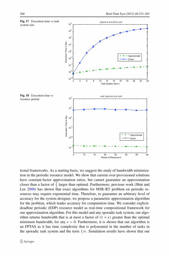
260 Real-Time Syst (2012) 48:223–263

Fig. 17 Execution time vs tasksystem size

Fig. 18 Execution time vsresource period

tional frameworks. As a starting basis, we suggest the study of bandwidth minimiza-tion in the periodic resource model. We show that current over-provisioned solutionshave constant-factor approximation ratios, but cannot guarantee an approximationcloser than a factor of 3

2 larger than optimal. Furthermore, previous work (Shin andLee 2008) has shown that exact algorithms for MIB-RT problem on periodic re-sources may require exponential time. Therefore, to guarantee an arbitrary level ofaccuracy for the system designer, we propose a parametric approximation algorithmfor the problem, which trades accuracy for computation time. We consider explicit-deadline periodic (EDP) resource model as real-time compositional framework forour approximation algorithm. For this model and any sporadic task system, our algo-rithm returns bandwidth that is at most a factor of (1 + ε) greater than the optimalminimum bandwidth, for any ε > 0. Furthermore, it is shown that our algorithm isan FPTAS as it has time complexity that is polynomial in the number of tasks inthe sporadic task system and the term 1/ε. Simulation results have shown that our

Real-Time Syst (2012) 48:223–263 261

approximation algorithm is effective at reducing the relative error over syntheticallygenerated tasks, while maintaining a low runtime complexity.

We believe that the attainment of parametric approximation algorithms for MIB-RT problem under a variety of compositional frameworks will provide a real-timecomponent designer with a valuable choice in determining how much interface band-width to trade for decreased speed-of-analysis. Extending the work contained in thispaper to more general task models (e.g., generalized multiframe tasks (Baruah et al.1999)) remains as future work. Furthermore, we expect that parametric approxima-tion algorithms for MIB-RT on uniprocessor frameworks will also extend to multi-processor compositional frameworks (e.g., Shin et al. 2008).

Acknowledgements We are sincerely thankful to the reviewers for the detailed comments, corrections,and insightful directions which helped us to improve the quality of the article. This research has beensupported in part by a National Science Foundation CAREER Award (CNS-0953585) and a grant fromWayne State University’s Office of Vice President of Research.

References

Albers K, Slomka F (2004) An event stream driven approximation for the analysis of real-time systems.In: Proceedings of the EuroMicro conference on real-time systems. IEEE Computer Society Press,Catania, pp 187–195

Albers K, Bodmann F, Slomka F (2008) Advanced hierarchical event-stream model. In: Proceedings ofthe EuroMicro conference on real-time systems. IEEE Computer Society, Prague, pp 211–220

Almeida L, Pedreiras P (2004) Scheduling within temporal partitions: response-time analysis and serverdesign. In: EMSOFT ’04: Proceedings of the 4th ACM international conference on embedded soft-ware. ACM, New York, pp 95–103. DOI:http://doi.acm.org/10.1145/1017753.1017772

Baruah S, Howell R, Rosier L (1990) Algorithms and complexity concerning the preemptive schedulingof periodic, real-time tasks on one processor. Real-Time Systems: The International Journal of Time-Critical Computing 2:301–324

Baruah S, Mok A, Rosier L (1990) Preemptively scheduling hard-real-time sporadic tasks on one pro-cessor. In: Proceedings of the 11th real-time systems symposium. IEEE Computer Society Press,Orlando, pp 182–190

Baruah S, Howell R, Rosier L (1993) Feasibility problems for recurring tasks on one processor. TheorComput Sci 118(1):3–20

Baruah S, Chen D, Gorinsky S, Mok A (1999) Generalized multiframe tasks. Time-Critical Comput Syst17(1):5–22

Bini E, Buttazzo G (2004) Biasing effects in schedulability measures. In: Proceedings of the 16th EuroMi-cro conference on real-time systems. IEEE Computer Society, Los Alamitos, pp 196–203

Davis RI, Burns A (2005) Hierarchical fixed priority pre-emptive scheduling. In: Proceedings of the IEEEreal-time systems symposium. IEEE Computer Society, Miami, pp 389–398

de Alfaro L, Henzinger TA (2001a) Interface automata. In: Proceedings of the ninth annual symposium onfoundations of software engineering (FSE). ACM Press, Vienna, pp 109–120

de Alfaro L, Henzinger TA (2001b) Interface theories for component-based design. In: EMSOFT ’01:Proceedings of the first international workshop on embedded software. Springer, London, pp 148–165

Deng Z, Liu J (1997) Scheduling real-time applications in an open environment. In: Proceedings of theeighteenth real-time systems symposium. IEEE Computer Society Press, San Francisco, pp 308–319

Easwaran A (2007) Compositional schedulability analysis supporting associativity, optimality, dependencyand concurrency. PhD dissertation, University of Pennsylvania, Department of Computer and Infor-mation Science

Easwaran A, Anand M, Lee I (2007) Compositional analysis framework using EDP resource models. In:Proceedings of the IEEE real-time systems symposium. IEEE Computer Society, Tuscon, pp 129–138

262 Real-Time Syst (2012) 48:223–263

Eisenbrand F, Rothvoß T (2010) EDF-schedulability of synchronous periodic task systems is coNP-hard.In: Proceedings of the annual ACM-SIAM symposium on discrete algorithms

Feng XA, Mok A (2002) A model of hierarchical real-time virtual resources. In: Proceedings of the IEEEreal-time systems symposium. IEEE Computer Society, Los Alamitos, pp 26–35

Fisher N (2008) Approximation algorithms for compositional real-time systems: Trading bandwidth forspeed-of-analysis. In: Proceedings of the workshop on compositional theory and technology for real-time embedded systems. IEEE Computer Society Press, Barcelona

Fisher N (2009) An FPTAS for interface selection in the periodic resource model. In: Proceedings of the17th international conference on real-time and network systems. Paris, France

Fisher N, Dewan F (2009) Approximate bandwidth allocation for compositional real-time systems. In:Proceedings of the 21st EuroMicro conference on real-time systems. IEEE Computer Society Press,Dublin

Henzinger TA, Matic S (2006) An interface algebra for real-time components. In: RTAS ’06: Proceedingsof the 12th IEEE real-time and embedded technology and applications symposium. IEEE ComputerSociety, Washington, DC, pp 253–266

Kuo TW, Li CH (1998) A fixed priority driven open environment for real-time applications. In: Proceed-ings of the IEEE real-time systems symposium. IEEE Computer Society Press, Madrid, pp 256–267

Lehoczky J, Sha L, Ding Y (1989) The rate monotonic scheduling algorithm: Exact characterization andaverage case behavior. In: Proceedings of the real-time systems symposium—1989. IEEE ComputerSociety Press, Santa Monica, pp 166–171

Lipari G, Baruah S (2000) Efficient scheduling of real-time multi-task applications in dynamic systems.In: Proceedings of the real-time technology and applications symposium. IEEE Computer SocietyPress, Washington, pp 166–175

Lipari G, Bini E (2003) Resource partitioning among real-time applications. In: Proceedings of the Eu-roMicro conference on real-time systems. IEEE Computer Society, Porto, pp 151–160

Lipari G, Carpenter J, Baruah S (2000) A framework for achieving inter-application isolation in multipro-grammed, hard real-time environments. In: Proceedings of the real-time systems symposium. IEEEComputer Society Press, Orlando, pp 217–226

Mok AK (1983) Fundamental design problems of distributed systems for the hard-real-time environment.PhD thesis, Laboratory for Computer Science, Massachusetts Institute of Technology. Available asTechnical Report No MIT/LCS/TR-297

Mok A (1988) Task management techniques for enforcing ED scheduling on a periodic task set. In: Proc.5th IEEE workshop on real-time software and operating systems. Washington DC, pp 42–46

Mok A, Feng X, Chen D (2001) Resource partition for real-time systems. In: 7th IEEE real-time technol-ogy and applications symposium (RTAS ’01). IEEE Press, New York, pp 75–84

Rajkumar R, Juvva K, Molano A, Oikawa S (2001) Resource kernels: a resource-centric approach toreal-time and multimedia systems. In: Readings in multimedia computing and networking. MorganKaufmann, San Francisco, pp 476–490

Regehr J, Stankovic JA (2001) HLS: A framework for composing soft real-time schedulers. In: Proceedingsof the 22nd IEEE real-time systems symposium (RTSS 2001). London, UK, pp 3–14

Saewong S, Rajkumar R, Lehoczky JP, Klein MH (2002) Analysis of hierarchical fixed-priority scheduling.In: Proceedings of the EuroMicro conference on real-time systems. IEEE Computer Society Press,Vienna, pp 173–181

Shin I, Lee I (2003) Periodic resource model for compositional real-time guarantees. In: Proceedings ofthe IEEE real-time systems symposium. IEEE Computer Society, Los Alamitos, pp 2–13

Shin I, Lee I (2004) Compositional real-time scheduling framework. In: Proceedings of the IEEE real-timesystems symposium. IEEE Computer Society, Los Alamitos, pp 57–67

Shin I, Lee I (2008) Compositional real-time scheduling framework with periodic model. ACM TransEmbed Comput Syst 7(3):30:1–30:39

Shin I, Easwaran A, Lee I (2008) Hierarchical scheduling framework for virtual clustering of multipro-cessors. In: Proceedings of the EuroMicro conference on real-time systems. IEEE Computer SocietyPress, Prague, pp 181–190

Thiele L, Chakraborty S, Naedele M (2000) Real-time calculus for scheduling hard real-time systems. In:Proceedings of IEEE international symposium on circuits and systems (ISCAS) Geneva, Switzerland,pp 101–104

Thiele L, Wandeler E, Stoimenov N (2006) Real-time interfaces for composing real-time systems. In:Proceedings of the 6th ACM and IEEE international conference on embedded software (EMSOFT),pp 34–43

Real-Time Syst (2012) 48:223–263 263

Vazirani VV (2001) Approximation algorithms. Springer, BerlinWandeler E, Thiele L (2005) Real-time interfaces for interface-based design of real-time systems with

fixed priority scheduling. In: EMSOFT ’05: Proceedings of the 5th ACM international conference onEmbedded software. ACM, New York, pp 80–89. DOI:http://doi.acm.org/10.1145/1086228.1086246

Wandeler E, Thiele L (2006) Interface-based design of real-time systems with hierarchical scheduling. In:IEEE real time technology and applications symposium, San Jose, CA, pp 243–252

Nathan Fisher is an Assistant Professor in the Department of Com-puter Science at Wayne State University. He received his Ph.D. fromthe University of North Carolina at Chapel Hill in 2007, his M.S. de-gree from Columbia University in 2002, and his B.S. degree from theUniversity of Minnesota in 1999, all in computer science. His researchinterests are in real-time and embedded computer systems, parallel anddistributed algorithms, resource allocation, algorithmic mechanism de-sign, and approximation algorithms.

Farhana Dewan is a Ph.D. student in the Department of ComputerScience at Wayne State University in Detroit, Michigan. She did herM.S. degree in computer science from Wayne State University in 2011and received her B.S. degree in computer science and engineering fromBangladesh University of Engineering and Technology in 2006. Sheis currently working with Dr. Nathan Fisher on her research focus ofcompositional real-time systems.