ESRM 430QUIZ 3

A B

Image A is an example of Nearest Neighbor Interpolation technique and image B is an example of Bilinear Interpolation

1. Which technique leaves pixel values unchanged? _________2. Geometry of linear features is preserved with _______________; thus, this type of

interpolation is most suitable for feature classification.

5/21/2013 ESRM430

Nearest Neighbor Bilinear Interpolation Cubic Convolution

MrSID

GeoTIFF

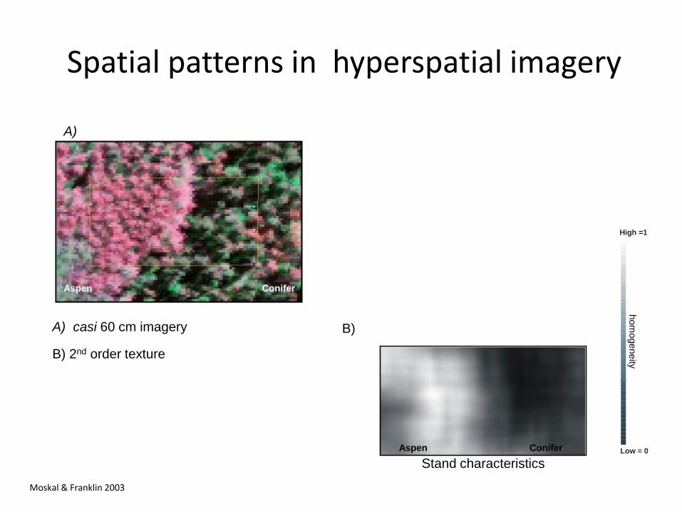
Spatial patterns in hyperspatial imagery

20 m

40 m

Aspen Conifer

A) casi 60 cm imagery

B) 2nd order texture

A)

Aspen Conifer

Stand characteristics

Aspen Conifer

High =1

Low = 0

hom

ogeneity

B)

Moskal & Franklin 2003

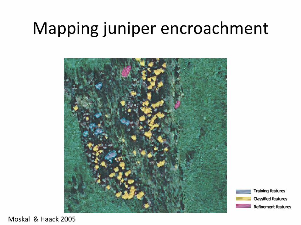
Mapping juniper encroachment

Training features

Classified features

Refinement features

Moskal & Haack 2005

Automated tree stems identification

A B

Training features

Classified features

Refinement features

Moskal & Haack 2005

Moskal & Haack 2005

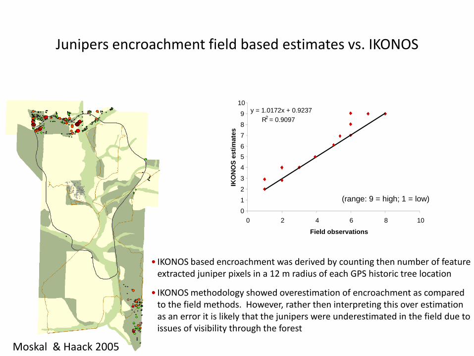
Junipers encroachment field based estimates vs. IKONOS

(range: 9 = high; 1 = low)

y = 1.0172x + 0.9237

R2 = 0.9097

0

1

2

3

4

5

6

7

8

9

10

0 2 4 6 8 10

Field observationsIK

ON

OS

esti

mate

s

• IKONOS based encroachment was derived by counting then number of feature extracted juniper pixels in a 12 m radius of each GPS historic tree location

• IKONOS methodology showed overestimation of encroachment as compared to the field methods. However, rather then interpreting this over estimation as an error it is likely that the junipers were underestimated in the field due to issues of visibility through the forest

Moskal & Haack 2005

Exercise (about 20 minutes)

• Instructor lead exercise to demonstrates how a mean filter, co-occurrence matrix and semivariogram are calculated based on the following subset image

1 0 0

1 3 0

1 1 1

0 1 2 3

0

1

2

3

‘Textures’ from tree density - dense to sparse

Baringo, KenyaA

B

C

A

B

C

Extra Credit (email to TA by May 27th)

1. Calculate semivariance using W to EW direction– List and count the pairs based on lag distance 1 and 2– Calculate semivariance

• For each pair separated by 1 lag, calculate the difference, and then square the difference.

• Sum up all the differences and divide by twice the number of pairs

• This gives the similarity measure g(h) for the variogram for that particular lag increment or distance.

• The same is done for other lag distances– Draw a semivariogram– Outline sill, nugget and range– Discuss forest inventory implications

1 0 0

1 3 0

1 1 1