Embed Size (px)
Citation preview
INTERNATIONAL JOURNAL FOR NUMERICAL METHODS IN ENGINEERINGInt. J. Numer. Meth. Engng 2011; 86:1339–1359Published online 25 January 2011 in Wiley Online Library (wileyonlinelibrary.com). DOI: 10.1002/nme.3107
A 3D finite element approach for the coupled numerical simulationof electrochemical systems and fluid flow
Georg Bauer1, Volker Gravemeier1,2 and Wolfgang A. Wall1,∗,†
1Institute for Computational Mechanics, Technische Universität München, Boltzmannstr. 15,
D-85747 Garching, Germany2Emmy Noether Research Group ‘Computational Multiscale Methods for Turbulent Combustion’,
Technische Universität München, Boltzmannstr. 15, D-85747 Garching, Germany
SUMMARY
A comprehensive finite element method for three-dimensional simulations of stationary and transientelectrochemical systems including all multi-ion transport mechanisms (convection, diffusion and migration)is presented. In addition, non-linear phenomenological electrode kinetics boundary conditions are accountedfor. The governing equations form a set of coupled non-linear partial differential equations subject to analgebraic constraint due to the electroneutrality condition. The advantage of a convective formulation ofthe ion-transport equations with respect to a natural application of homogeneous flux boundary conditionsis emphasized. For one of the numerical examples, an analytical solution for the coupled problem isprovided, and it is demonstrated that the proposed computational approach is robust and provides accurateresults. Copyright � 2011 John Wiley & Sons, Ltd.
Received 28 December 2009; Revised 2 September 2010; Accepted 10 November 2010
KEY WORDS: finite element method; ion transport; electrolyte solution; computational electrochemistry;transient convection–diffusion–migration equation; electroneutrality condition
1. INTRODUCTION
The inclusion of ion-transport phenomena plays a fundamental role for the modeling of manyelectrochemical systems. Typically, three different ion-transport mechanisms are considered indilute electrolyte solutions, see, e.g. [1]: convection (movement with bulk electrolyte solution),diffusion (movement caused by concentration gradients) and migration (movement caused by theapplied electric field). In this work, we focus on electrochemical systems where the influence ofconvection is not negligible. As an example, we name electrodeposition, which is an importantand widely used electrochemical technique for coating electrically conductive objects with layersof metal by using electrical current. In many industrial plating baths, it is aimed at keeping theelectrolyte solution well mixed by using different jet systems and stirring devices. Rotationallysymmetric parts to be plated are usually also rotated to achieve uniform plating results. As aconsequence, quite complex, often turbulent flow conditions arise, directly influencing the ion-transport processes inside the electrolyte solution. Hence, a mathematical model describing suchelectrochemical systems has to take into account the apparent coupling to fluid flow.
Various numerical approaches for the simulation of multi-ion transport in dilute electrolytesolutions have been developed over the last decades. A Lattice-Boltzmann model for studying
∗Correspondence to: Wolfgang A. Wall, Institute for Computational Mechanics, Technische Universität München,Boltzmannstr. 15, D-85747 Garching, Germany.
†E-mail: [email protected]
Copyright � 2011 John Wiley & Sons, Ltd.

1340 G. BAUER, V. GRAVEMEIER AND W. A. WALL
electrochemical processes influenced by all the three transport mechanisms was proposed in [2]for two-dimensional problems. Mesh-free numerical schemes were used in [3]. A finite-differencemethod with upwinding was developed in [4] for the simulation of convection-dominated multi-iontransport. Using that method, various two-dimensional electrochemical systems including convec-tion, e.g. parallel-plate electrochemical reactors [4, 5], a backward-facing step [4] and cavities inlaminar shear flow [6] were studied. A multi-dimensional upwinding method for the analysis ofmulti-ion electrolytes controlled by diffusion, convection and migration was proposed in [7]. It wasused to perform steady-state studies for a two-dimensional parallel plane flow channel. Recently, afractional-step method proposed in [8] for solving two-dimensional diffusion–migration problemson irregular domains with moving boundaries was extended to three space dimensions in [9]. Theresulting method is first-order accurate in time and second-order accurate in space using a finitevolume approach for the spatial discretization. Convection was neglected there, since their focuswas on semiconductor applications with very small length scales smaller than 1 �m. Anotherfractional-step algorithm had been developed earlier in [10] using a finite-difference scheme forspatial discretization. Instationary mass-transfer processes in a 3D-model of an electrochemicalsensor were investigated in [11] using a finite volume approach. All of the three ion-transportmechanisms were addressed in that study, but only the concentration field of one single reactivespecies was considered. In all investigations, the species concentration at the electrode surface wasassumed to be zero. The electric potential was computed by solving a Poisson–Boltzmann equation.
The finite element method (FEM) has also been used already for the spatial discretization ofdifferent electrochemical problems including ionic mass transport: in [12], a finite element methodwas used to simulate secondary current-density distributions in three-dimensional microchannels.However, the model used in [12] did not account for migration, and a constant conductivity of theelectrolyte solution was assumed. Ion-diffusion mechanisms in porous media were modeled in [13],using the Nernst–Planck/Poisson system of equations. Only diffusion and migration were consid-ered in the ion-transport model. The governing equations were discretized in space using a finiteelement method. Applying a commercial finite element software, a rotating cylinder Hull cell wasinvestigated in [14]. For computing steady-state current distributions, a 2D axial-symmetric modelwas used. Mass transport was modeled using a Nernstian diffusion layer expression and assumingTafel kinetics at the working electrode. Only the concentration of a single ionic species was consid-ered, and no flow field was computed. An adaptive multilevel finite element algorithm was proposedin [15] and applied for solving various controlled current experiments in one spatial dimension. Astabilized finite element approach for ionic transport was proposed in [16] for the simulation ofelectrophoresis separation in one and two space dimensions. The popular drift-diffusion model fordescribing the transport of charge carriers within semiconductor devices exhibits also strong simi-larities to the governing equations of multi-ion transport in dilute electrolyte solutions. In [17], astabilized finite element method was used for the spatial discretization of drift-diffusion equations.Within that study, the large-scale parallel performance of an algebraic multigrid preconditioner wasinvestigated.
To the authors’ best knowledge, no three-dimensional finite element method has been proposedso far for robust and accurate simulations of multi-ion transport in dilute electrolyte solutionsincluding all three transport mechanisms (convection, diffusion and migration) and (non-linear)reaction kinetics at the same time. In addition, we use the finite element method as a generalapproach for discretization, including the Navier–Stokes equations that govern the fluid flowcoupled to the electrochemical system. We successfully developed finite element methods forconvection–diffusion–reaction equations (see, e.g. [18]), incompressible flow (see, e.g. [19–21])and, recently, for (turbulent) variable-density flow at low Mach number in [22, 23].
The outline of this study is as follows. In Section 2, we present the governing equations for multi-ion transport in dilute electrolyte solutions. Our computational approach based on a finite elementmethod is then given in Section 3. The numerical method is tested for various numerical examplesin Section 4. For one three-dimensional example, we even provide an analytical solution, beinga valuable contribution for code-validation purposes in computational electrochemistry. Finally,conclusions are drawn in Chapter 5.
Copyright � 2011 John Wiley & Sons, Ltd. Int. J. Numer. Meth. Engng 2011; 86:1339–1359DOI: 10.1002/nme

3D FINITE ELEMENT APPROACH FOR COUPLED ELECTROCHEMICAL SYSTEMS 1341
2. MULTI-ION TRANSPORT IN DILUTE ELECTROLYTE SOLUTIONS
Electrolyte flow and multi-ion transport in a polygonally-shaped and bounded domain �⊂Rd ,where d�3 is the number of space dimensions, is considered for the time interval [0,T ]. Theboundary of � is denoted by �� and assumed sufficiently smooth. The closure of � is defined by� :=�∪��. The incompressible Navier–Stokes equations provide an adequate model to describethe flow of a dilute electrolyte solution in an electrochemical cell at a macroscopic scale (see, e.g.[1]). For dilute solutions, as considered here, concentrations of contained ionic species are verylow compared to the solute. As a result, values for density and viscosity are typically only slightlydifferent to those of the pure solute. Typically, the latter is water, which is governing the flowbehavior of the whole electrolyte solution. The solution variables are the velocity field u and thepressure p, which are governed by
�u
�t+u·∇u−2�∇ ·e(u)+∇ p = b in �×(0,T ), (1)
∇ ·u = 0 in �×(0,T ), (2)
where � denotes the kinematic viscosity, b the specific volume force and e(u) the symmetric strainrate tensor given by
e(u)= 12 (∇u+(∇u)T ). (3)
Based on the partition ��=�D ∪�N with �D ∩�N �=∅, appropriate boundary conditions read:
u = uD on �D ×(0,T ), (4)
(−pI+2�e(u)) ·n = t on �N ×(0,T ). (5)
Here, uD is the velocity prescribed at the boundary part �D, n the unit outer normal to the boundaryand t the boundary traction at �N. Finally, an initial condition in the form
u=u0 in �×{0} (6)
is required for instationary flow problems with u0 being a solenoidal initial velocity field.Based on mass conservation, for each ionic species k =1, . . . ,m present in an electrolyte solution,
a non-linear partial differential equation is obtained, describing temporal and spatial variation ofits molar concentration ck :
�ck
�t+∇ ·Nk =0 in �×(0,T ), (7)
with the total flux given by
Nk := ( cku︸︷︷︸convection
− Dk∇ck︸ ︷︷ ︸diffusion
− zk�k Fck∇�︸ ︷︷ ︸migration
). (8)
In literature, Equation (7) is also often referred to as Nernst–Planck equation. Here, Dk is thediffusion coefficient of ionic species k with respect to the solute, zk is the valence (charge number),�k the mobility constant, F Faraday’s constant (96 485 C/mol), � the electric potential insidethe electrolyte solution and u the velocity field governed by the incompressible Navier–Stokesequations. Thus, the convective term establishes a one-way coupling of fluid flow to each ion-transport equation. As usual in dilute-solution theory, we express the mobility constant �k in termsof diffusivity Dk , temperature T and the universal gas constant R by using the Nernst–Einsteinrelation
�k = Dk
RT. (9)
Copyright � 2011 John Wiley & Sons, Ltd. Int. J. Numer. Meth. Engng 2011; 86:1339–1359DOI: 10.1002/nme

1342 G. BAUER, V. GRAVEMEIER AND W. A. WALL
However, for brevity of notation, we keep using �k in subsequent formulae. An isothermal assump-tion is justified for the applications considered here, since the temperature of the electrolyte solutionis usually kept constant by some external thermal control. In addition, energy dissipation dueto ohmic losses (Joule heating) usually does not cause significant temperature changes for mostelectrodeposition problems. For these applications, electric currents passing the electrochemicalcells are typically low enough to confirm this modeling assumption. In electrochemical systems,reactions are typically restricted to electrode surfaces. Thus, no homogeneous chemical reactionsinside the bulk solution need to be taken into account, leading to a zero right-hand side in (7). Fora solenoidal velocity field u, Equation (7) can be converted from the conservative form (7) intothe following convective form:
�ck
�t+u·∇ck +∇ ·Nd+m
k =0 in �×(0,T ), (10)
where
Nd+mk :=−Dk∇ck −zk�k Fck∇�. (11)
Note that for neutral species (zk =0) Equation (10) reduces to a convection–diffusion equation,since non-charged particles are not influenced by the electric field E given by the negative gradientof the electric potential via E=−∇�. Since the electric potential � is an additional unknown scalarfield in (7) and (10), beside the ionic species concentrations ck , the system of equations is typicallyclosed with the so-called electroneutrality condition. This condition is an algebraic constraintoriginating from the assumption that the electrolyte solution is locally electrically neutral:
m∑k=1
zkck =0 in �×[0,T ]. (12)
As a consequence, at least two ionic species with opposite charges are required for modelingelectrochemical systems. The special case m =2 corresponds to the dissociation of a single saltand is usually referred to as binary electrolyte.
For the transient case, initial conditions for k =1, . . . ,m,
ck =c0k in �×{0}, (13)
have to be specified, which obey the electroneutrality condition. To specify boundary conditionsfor each ionic species k, the partition ��=�D,k ∪�N,k ∪�E,k is considered. The three boundaryregions are assumed to be pairwise disjoint. We note that the partitions do not have to be the samefor each species k. On �D,k , essential (or Dirichlet) boundary conditions as
ck =gk on �D,k ×(0,T ) (14)
are applied. A typical example is an inflow boundary where the composition of the electrolytesolution entering the domain is known. At �N,k , the negative normal flux caused by migration anddiffusion is prescribed:
−Nd+mk ·n=hk on �N,k ×(0,T ). (15)
Here, n denotes the unit outer normal vector at the boundary �N,k . Finally, electrode surfaces arerepresented by the boundary part �E,k , which can be further subdivided into any number of anodicand cathodic parts. There, electrochemical reaction models for reactive ionic species are includedinto the mathematical problem formulation. In this paper, we focus on the case of only one reactingspecies (without loss of generality this species is always considered the first one, i.e. k =1, in thenumerical examples). An important quantity for characterizing electrochemical systems is the totalcurrent density,
i= Fm∑
k=1zkNk = F
m∑k=1
zkNd+mk , (16)
Copyright � 2011 John Wiley & Sons, Ltd. Int. J. Numer. Meth. Engng 2011; 86:1339–1359DOI: 10.1002/nme

3D FINITE ELEMENT APPROACH FOR COUPLED ELECTROCHEMICAL SYSTEMS 1343
which is derived from the ion mass fluxes. Note that convection does not contribute to the currentdensity due to the electroneutrality condition. At electrode surfaces, the normal component in =i·n is of special interest, since it corresponds to the rate of electrochemical reaction. Thus, forelectroplating applications, in is directly proportional to the deposition rate at the cathode. Inertspecies have zero mass flux at these boundaries. Thus, the boundary condition reads
−Nd+mk ·n= jk :=
⎧⎨⎩
0 inert ionic species,
−in
zk Freactive ionic species.
(17)
The normal current density in on the associated boundary parts is determined by some (oftennon-linear) kinetic model that typically depends on the solution variables. An important exampleis the Butler–Volmer law in the form specified in [1]:
in = i0
(ck
c∞k
)� [exp
(�a F
RT(V −�)
)−exp
(−�c F
RT(V −�)
)]. (18)
The additional parameters involved are the exchange current density i0, some reference concentra-tion for the reactive ionic species c∞
k , an exponent � for weighting the concentration dependency, ananodic constant �a , a cathodic constant �c and the overpotential V −�, with V being the potentialapplied on the metal side of the electrode.
Equations (10) together with (11) and initial and boundary conditions define a volume-coupledsystem of non-linear partial differential equations subjected to an algebraic constraint givenin (12). In the following section, we present a finite element method for the numerical solutionof this system.
3. COMPUTATIONAL APPROACH
3.1. Weak problem formulation
With H1(�)⊂ L2(�), we denote the usual Sobolev space of square-integrable functions in � thatpossess a weak first derivative. With respect to each ionic species concentration ck , we define thespace
Sk :={ck ∈ H1(�)|ck =gk on �D,k} (19)
of admissible trial solutions satisfying the Dirichlet boundary conditions (14). The correspondingspaces of weighting (or test) functions for k =1, . . . ,m are defined by
Vk :={wk ∈ H1(�)|wk =0 on �D,k}. (20)
With respect to the electric potential � two spaces of functions,
S� :={�∈ H1(�)}, (21)
and
V� :={�∈ H1(�)}, (22)
are introduced for admissible trial solutions and test functions, respectively. Note that both spacescoincide, since no Dirichlet boundary conditions for the electric potential are applied. When onlyboundary conditions of type (14) and (15) are considered, the electric potential � is only definedup to a constant. For getting a unique solution, a point in � has to be chosen where a referencevalue for the electric potential is prescribed. In that case, formally, the quotient spaces S�/R andV�/R have to be used instead, where all functions that differ only by a constant are groupedtogether in corresponding equivalence classes. Hence, two functions that differ only by a constantare interpreted as the same function in these spaces.
Copyright � 2011 John Wiley & Sons, Ltd. Int. J. Numer. Meth. Engng 2011; 86:1339–1359DOI: 10.1002/nme
1344 G. BAUER, V. GRAVEMEIER AND W. A. WALL
Now, we consider the ion-transport equations (10) for k =1, . . . ,m. Multiplication with wk ∈Vkand integration over � gives∫
�wk
�ck
�td�+
∫�
wku·∇ck d�+∫
�wk∇ ·Nd+m
k d�=0 ∀wk ∈Vk .
After application of integration by parts to the third term on the left-hand side, using wk =0 on�D,k and inserting (15) and (17), the variational formulation reads(
wk,�ck
�t
)+(wk,u·∇ck)−(∇wk,Nd+m
k )−(wk, jk)�E,k = (wk,hk)�N,k ∀wk ∈Vk . (23)
Here, (· , ·) := (· , ·)� denotes the L2-inner product on �. The L2-inner products on �N,k and �E,kare denoted with (· , ·)�N,k and (· , ·)�E,k , respectively. The third term in (23) reads
−(∇wk,Nd+mk )= Dk(∇wk,∇ck)+zk�k F(∇wk,ck∇�). (24)
At this point it is worth mentioning that choosing the convective formulation (10) is beneficialw.r.t. the application of mass-flux boundary conditions. Performing another integration by parts on(23) leads to(
wk,�ck
�t+u·∇ck +∇ ·Nd+m
k
)−(wk,Nd+m
k ·n+ jk)�E,k = (wk,Nd+mk ·n+hk)�N,k ∀wk ∈Vk . (25)
Thus, when the solution of the weak form is smooth enough to fulfill the original partial differentialequation, the flux boundary conditions (15) and (17) are naturally fulfilled. Typically, at walls,a zero total flux in normal direction is demanded. Since u·n=0 at impermeable walls, there isno mass flux due to convection in that case. Consequently, the normal flux Nd+m
k ·n caused bydiffusion and migration has to be zero, i.e. hk =0. In turn, the term w.r.t. �N,k vanishes in (23).Thus, no boundary integral has to be computed resulting in simple ‘doing nothing’ conditionsin that case. This is especially useful at outflow boundaries, where it is impossible to prescribethe total flux, since the contribution due to convection is a priori unknown. Usually, Nd+m
k ·n=0is demanded, which is again fulfilled by the method in a natural way. As a consequence, onlyDirichlet boundary conditions and boundary parts with hk �=0 or jk �=0 require to be explicitlyaccounted for in the computational framework.
Since the electroneutrality condition (12) is the equation for the electric potential (although itdoes not explicitly contain �), it is multiplied with a corresponding test function �∈V�. Thisapproach is consistent with the performed weighting of the ion-transport residuals as well as withthe treatment of other closing equations for the electric potential within a finite element formulation(see, e.g. [13, 16]). After integration over the computational domain the weighted residual form of(12) reads: (
�,m∑
k=1zkck
)=
m∑k=1
zk(�,ck)=0 ∀�∈V�. (26)
In summary, the weak form of the instationary multi-ion-transport problem is given as: for eachtime t ∈ (0,T ) find c1(., t)∈S1, . . . ,cm(., t)∈Sm and �(., t)∈S�, such that
Bk(wk,ck,�) =Fk(wk) ∀wk ∈Vk, k =1, . . . ,m (27)
m∑k=1
zk(�,ck) = 0 ∀�∈V�, (28)
where
Bk(wk,ck,�) :=(
wk,�ck
�t
)+(wk,u·∇ck)+ Dk(∇wk,∇ck)+zk�k F(∇wk,ck∇�)
−(wk, jk(ck,�))�E,k
Copyright � 2011 John Wiley & Sons, Ltd. Int. J. Numer. Meth. Engng 2011; 86:1339–1359DOI: 10.1002/nme
3D FINITE ELEMENT APPROACH FOR COUPLED ELECTROCHEMICAL SYSTEMS 1345
and
Fk(wk) := (wk,hk)�N,k .
3.2. Finite element discretization
Via restriction of the involved function spaces to finite-dimensional subspaces Vhk ⊂Vk , Sh
k ⊂Sk ,Vh
� ⊂V� and Sh� ⊂S� we derive a discrete version of the variational problem: for each time
t ∈ (0,T ) find ch1 (., t)∈Sh
1, . . . ,chm(., t)∈Sh
m and �h(., t)∈Sh�, such that
Bk(whk ,ch
k ,�h) =Fk(whk ) ∀wh
k ∈Vhk , k =1, . . . ,m (29)
m∑k=1
zk(�h,chk ) = 0 ∀�h ∈Vh
�. (30)
By using a nodal basis {N hi , i =1, . . . ,nnod}, where N h
i denotes the shape function associated withnode i , the finite-element approximation ch
k to the concentration ck reads
chk =
nnod∑i=1
N hi ck,i (31)
with ck,i being the unknown concentration value of ionic species k at node i . The latter arearranged in the nodal solution vector ck . The same shape functions are also used to express �h ,velocity field uh and pressure field ph in terms of basis functions and nodal unknowns. Thecorresponding solution vectors are denoted by U, u and p, respectively. We use matching spatialdiscretizations for both fluid and electrochemistry system with the same ansatz-function order.Since equal-order shape functions for velocity and pressure are used, stabilization techniques arerequired for circumventing the inf–sup condition (see, e.g. [19, 21, 24]). An adequate stabilizationfor the case of dominating convection is ensured as well. For completeness, we summarize thestabilized finite element formulation of the Navier–Stokes equations that is solved: find ph ∈Sh
p,
uh ∈Shu such that
(qh,∇ ·uh)+(∇qh,�MRhM)=0, (32)(
vh,�uh
�t
)−(∇ ·vh, ph)+(ε(vh),2�ε(uh))+(∇ ·vh,�CR
hC)+(vh,uh ·∇uh)+(uh ·∇vh,�MRh
M)
= (vh,b)+(vh,hu)�N,u∀vh ∈Vhu. (33)
For details concerning this formulation, the reader is referred to, e.g. [19, 21]. In the following,however, the emphasis is on the numerical treatment of the electrochemistry part.
3.3. Non-linear matrix formulation of the electrochemistry model
For discretizing (29) in time, we apply the generalized trapezoidal rule, which is second-orderaccurate for �=0.5 (Crank–Nicolson scheme). The resulting set of non-linear equations withrespect to ionic species k at time step n+1 reads
Rn+1k (cn+1
k ,Un+1) := [M+��t(C(un+1)+ DkK)]cn+1k +��tEk(cn+1
k ,Un+1)
+��tIk(cn+1k ,Un+1)−��tfn+1
N −fnT =0 (34)
with fnT defined as
fnT := [M−(1−�)�t(C(un)+ DkK)]cn
k −(1−�)�tEk(cnk ,U
n)−(1−�)�tIk(cnk ,U
n)−(1−�)�tfnN
and �t being the time-step length. Here, M denotes the mass matrix, C(un+1) the matrix arisingfrom the discretization of the convective term, K the matrix emanating from the diffusive term, and
Copyright � 2011 John Wiley & Sons, Ltd. Int. J. Numer. Meth. Engng 2011; 86:1339–1359DOI: 10.1002/nme

1346 G. BAUER, V. GRAVEMEIER AND W. A. WALL
Ek(cn+1k ,Un+1) denotes the non-linear migration term in its discretized form at time tn+1. Contribu-
tions due to mass-flux boundary conditions (15) and (17) are denoted by fn+1N and Ik(cn+1
k ,Un+1),respectively. The electroneutrality condition in discretized form reads
Rn+1EN (cn+1
1 , . . . ,cn+1m ) :=
m∑k=1
zkMcn+1k =0. (35)
Note that since the mass matrix M is regular, equation (35) is equivalent to a strong enforcementof the constraint condition at each node:
m∑k=1
zkcn+1k =0⇔M
m∑k=1
zkcn+1k =0. (36)
The resulting non-linear equation system at time step n+1 is given by
Rn+1(yn+1)=
⎡⎢⎢⎢⎢⎢⎢⎣
Rn+11 (cn+1
1 ,Un+1)
...
Rn+1m (cn+1
m ,Un+1)
Rn+1EN (cn+1
1 , . . . ,cn+1m )
⎤⎥⎥⎥⎥⎥⎥⎦
=
⎡⎢⎢⎢⎢⎢⎣
0
...
0
0
⎤⎥⎥⎥⎥⎥⎦ with yn+1 =
⎡⎢⎢⎢⎢⎢⎢⎣
cn+11
...
cn+1m
Un+1
⎤⎥⎥⎥⎥⎥⎥⎦
. (37)
It is solved via Newton’s method for all nodal unknowns collected in yn+1. The following iterationprocedure is executed until convergence is achieved:
Solve :�Rn+1(y)
�y
∣∣∣∣∣yn+1
i
�yn+1i =−Rn+1(yn+1
i ), (38)
Update : yn+1i+1 =yn+1
i +�yn+1i . (39)
As a result, in each iteration step i of the non-linear solution algorithm, a sparse linear equa-tion system (38) has to be solved for the solution increment �yn+1
i . Owing to the electroneu-trality condition, the resulting tangent matrix exhibits a saddle-point structure. For the numericalexamples in this paper, we use a direct sparse solver package [25]. For larger systems, iterativeprocedures in combination with efficient preconditioning techniques are required. An overviewof solution techniques for general saddle-point problems can be found in [26], for example. Forincluding a phenomenological electrode kinetics law given in the form in = f (ck,�), evaluation ofIk(cn+1
k ,Un+1) is required for establishing the right-hand side vector in Equation (38). In addition,the partial derivatives of Ik(cn+1
k ,Un+1) w.r.t. surface concentration and electric potential have tobe provided for computing the corresponding matrix contributions. These evaluations have to beimplemented to the elements on the boundary that are used for discretizing electrode surfaces. Morecomplex surface chemistry models are typically consisting of a coupled system of convection–diffusion–reaction equations to be solved at electrode surfaces. Thus, no single reaction law asdiscussed above is available. If such models have to be accounted for, it is necessary to extend ourpresent numerical approach. In that case, numerical methods as proposed in [9] can be applied forefficient coupling of governing surface and bulk equations.
3.4. One-way coupling fluid flow—electrochemistry
If convection has to be accounted for, a one-way coupling of fluid flow to ion transport has tobe appropriately performed. In each time step, we first solve the non-linear Navier–Stokes systemfor un+1 and pn+1. Afterwards, un+1 is transferred for solving the non-linear electrochemistryequations. Finally, the multi-ion transport problem is solved for the current time step. A sketch ofthe coupling algorithm is provided in Figure 1. The same order is also used for solving stationaryproblem formulations without proceeding in time. This one-way coupled approach is all that is
Copyright � 2011 John Wiley & Sons, Ltd. Int. J. Numer. Meth. Engng 2011; 86:1339–1359DOI: 10.1002/nme

3D FINITE ELEMENT APPROACH FOR COUPLED ELECTROCHEMICAL SYSTEMS 1347
Figure 1. One-way coupling fluid flow—electrochemistry.
needed for the current model. For future applications, however, the proposed coupling schemewill be extended to a two-way-coupled partitioned scheme. A possible application that requiressuch an extension is the consideration of electrode shape changes due to deposition processes.Furthermore, local electrolyte density and viscosity variations due to ion-concentration variationsnear the electrodes result in natural convection phenomena. Both effects influence the flow field, thefirst one due to a moving-boundary problem, the second one due to varying material parameters.Appropriate numerical methods for both problem classes were recently developed, see, e.g. [27, 28]for flows with moving boundaries and [22, 23] for variable-density approaches to fluid flow. Forelectrochemical problems where an isothermal assumption is not justified, a heat transport equationwould have to be solved additionally. For such problems, density, viscosity and diffusivity dependon the temperature. Furthermore, temperature variations also influence the mobility constant subjectto (9). Computational approaches for handling such temperature-dependent problem configurationswere already proposed and successfully tested in [22, 23].
4. NUMERICAL EXAMPLES
4.1. Analysis of a transient diffusion–migration problem in 3D
To demonstrate that our computational approach performs well for problems only governed bydiffusion and migration, we simulate instationary ion transport for a two-species system in thedomain �= (0,1)3 over a time interval [0,T ]. At all boundaries, zero flux conditions for both ionicspecies are prescribed. The material parameters are z1 =1, z2 =−2, D1 =0.008 and D2 =0.005.The initial concentration fields, fulfilling the electroneutrality condition at t =0, are given as:
c01(x, y, z) = 2.0+cos(x)cos(2y)cos(3z), (40)
c02(x, y, z) = − z1
z2c0
1(x, y, z). (41)
A visualization of the initial field c01 is provided in Figure 2. A similar configuration was investigated
in [29] as a 1D problem. The analytical solution of the problem specified in that work was thebasis for a more general extension to two spatial dimensions performed in [10]. Using similarmethods, the logical extension to three space dimensions is provided in the appendix to this paperas a special case of a more general analysis. The exact solution for the specified initial boundaryvalue problem reads:
c1(x, y, z, t) = 2.0+cos(x)cos(2y)cos(3z)e−14D2t , (42)
c2(x, y, z, t) = − z1
z2c1(x, y, z, t), (43)
F
RT�(x, y, z, t) = D2 − D1
z1 D1 −z2 D2ln
(c1(x, y, z, t)
c1(0,0,0, t)
), (44)
where �(0,0,0, t)=0 is fixed to define a reference level for the electric potential �. The factorF/RT remains arbitrary and is assumed to be 1.0 in this example. For studying the convergence
Copyright � 2011 John Wiley & Sons, Ltd. Int. J. Numer. Meth. Engng 2011; 86:1339–1359DOI: 10.1002/nme

1348 G. BAUER, V. GRAVEMEIER AND W. A. WALL
Figure 2. Initial cation concentration field c01 for the transient three-dimensional diffusion–migration
problem depicted on the discretization with element edge length h =0.1.
behavior in space and time, absolute errors are computed for each of the three unknown fields atthe time of interest using the L2-norm on �:
ek : = ‖chk −ck‖L2(�) for k ∈{1,2}, (45)
e� := ‖�h −�‖L2(�). (46)
Hexahedral elements with trilinear shape functions are used. A series of four uniform discretizationswith characteristic element edge lengths h =0.2,h =0.1,h =0.05 and h =0.025 are considered. Forthe temporal error being negligible compared to the error introduced by the spatial discretization,a small (constant) time-step size �t =0.005 is used. Using the Crank–Nicolson scheme (�=0.5), 20 time steps are performed. The computed errors depicted in Figure 3 show second-orderconvergence in space for both ionic species concentrations as well as for the electric potential.Note that (43) is reflected in the computed values for the absolute errors, leading to e1 =2e2 forthe given valences. When depicting relative instead of absolute errors, the curves for cation andanion would coincide. For investigating the temporal accuracy of our computational approach, thespatial error contributions have to be minimized. Owing to the approximation of cosine functionswith trilinear shape functions, the spatial error is dominating in this example. Hence, a very fineuniform discretization with h =0.01 has to be used for revealing the error contribution due to timediscretization. Different numbers of constant time steps are used to reach T =2.0, where the errormeasures introduced above are evaluated. The results for the Crank–Nicolson scheme are shownin Figure 4. As expected, second-order accuracy in time is observed for all physical fields.
4.2. Comparison with an analytical solution for electroplating
In [30], a steady-state solution for electroplating was specified for one spatial dimension. Themathematical model solved in [30] considers diffusion and migration within a binary electrolyte,the electroneutrality condition and non-linear boundary conditions of Butler–Volmer type for the
Copyright � 2011 John Wiley & Sons, Ltd. Int. J. Numer. Meth. Engng 2011; 86:1339–1359DOI: 10.1002/nme

3D FINITE ELEMENT APPROACH FOR COUPLED ELECTROCHEMICAL SYSTEMS 1349
10 10 1010
10
10
10
10
characteristic element length h
cation concentrationanion concentrationelectric potentialslope 2
Figure 3. Spatial convergence for cation concentration c1, anion concentration c2 and electric potential �.
10 10 10 10 10 10 1010
10
time step size
abso
lute
err
or in
L2 –n
orm
cation concentrationanion concentrationelectric potentialslope 2
Figure 4. Temporal convergence for cation concentration c1, anion concentration c2 and electric potential� using the Crank–Nicolson scheme.
electrode surfaces. Owing to the latter, this example is well suited for testing the numerical treatmentof non-linear electrode kinetics boundary conditions as proposed in Section 3. Additionally, thecapability of solving a stationary electrochemical problem is demonstrated here as well. Thematerial parameters are as follows: z1 =1, z2 =−1, D1 =5.0 and D2 =10.0. Instead of a one-dimensional geometry we consider the three-dimensional unit cube �= (0,1)3. A mesh consistingof 10×10×10 eight-noded hexahedrals with trilinear shape functions is used for the spatialdiscretization of the problem. The electrodes are located at the planes x1 =0 (anode) and x1 =1(cathode). The cation species is reacting at the electrodes, while the anion species is inert in thisexample. At both electrode surfaces, the Butler–Volmer law (18) is applied. The parameters forthe electrode kinetics are provided in Table I. On other boundary parts, zero mass flux for bothionic species is assumed. Since there are no Dirichlet boundary conditions present, we have to fixthe anion concentration at a point in order to establish a well-posed steady-state problem. We dothis at the center of the domain, demanding c2(0.5,0.5,0.5)=1.0.
Copyright � 2011 John Wiley & Sons, Ltd. Int. J. Numer. Meth. Engng 2011; 86:1339–1359DOI: 10.1002/nme
1350 G. BAUER, V. GRAVEMEIER AND W. A. WALL
Table I. Parameters for Butler–Volmer law used for the numerical solutionof a stationary electroplating problem.
Parameter c∞1 � �a �c i0 V
Anode 1.0 1.0 1.0 0.0 −1.0 1.0 (VA)Cathode 1.0 1.0 0.0 1.0 −1.0 0.0 (VC)
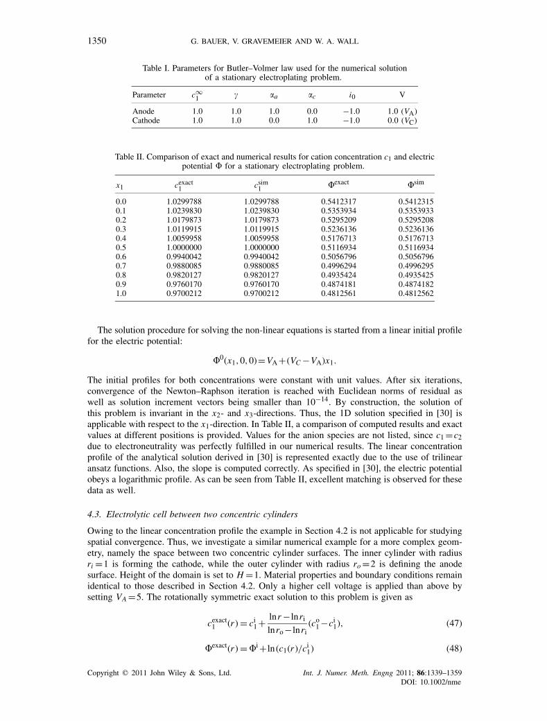
Table II. Comparison of exact and numerical results for cation concentration c1 and electricpotential � for a stationary electroplating problem.
x1 cexact1 csim
1 �exact �sim
0.0 1.0299788 1.0299788 0.5412317 0.54123150.1 1.0239830 1.0239830 0.5353934 0.53539330.2 1.0179873 1.0179873 0.5295209 0.52952080.3 1.0119915 1.0119915 0.5236136 0.52361360.4 1.0059958 1.0059958 0.5176713 0.51767130.5 1.0000000 1.0000000 0.5116934 0.51169340.6 0.9940042 0.9940042 0.5056796 0.50567960.7 0.9880085 0.9880085 0.4996294 0.49962950.8 0.9820127 0.9820127 0.4935424 0.49354250.9 0.9760170 0.9760170 0.4874181 0.48741821.0 0.9700212 0.9700212 0.4812561 0.4812562
The solution procedure for solving the non-linear equations is started from a linear initial profilefor the electric potential:
�0(x1,0,0)=VA +(VC −VA)x1.
The initial profiles for both concentrations were constant with unit values. After six iterations,convergence of the Newton–Raphson iteration is reached with Euclidean norms of residual aswell as solution increment vectors being smaller than 10−14. By construction, the solution ofthis problem is invariant in the x2- and x3-directions. Thus, the 1D solution specified in [30] isapplicable with respect to the x1-direction. In Table II, a comparison of computed results and exactvalues at different positions is provided. Values for the anion species are not listed, since c1 =c2due to electroneutrality was perfectly fulfilled in our numerical results. The linear concentrationprofile of the analytical solution derived in [30] is represented exactly due to the use of trilinearansatz functions. Also, the slope is computed correctly. As specified in [30], the electric potentialobeys a logarithmic profile. As can be seen from Table II, excellent matching is observed for thesedata as well.
4.3. Electrolytic cell between two concentric cylinders
Owing to the linear concentration profile the example in Section 4.2 is not applicable for studyingspatial convergence. Thus, we investigate a similar numerical example for a more complex geom-etry, namely the space between two concentric cylinder surfaces. The inner cylinder with radiusri =1 is forming the cathode, while the outer cylinder with radius ro =2 is defining the anodesurface. Height of the domain is set to H =1. Material properties and boundary conditions remainidentical to those described in Section 4.2. Only a higher cell voltage is applied than above bysetting VA =5. The rotationally symmetric exact solution to this problem is given as
cexact1 (r ) = ci
1 + lnr − lnri
lnro − lnri(co
1 −ci1), (47)
�exact(r ) = �i + ln (c1(r )/ci1) (48)
Copyright � 2011 John Wiley & Sons, Ltd. Int. J. Numer. Meth. Engng 2011; 86:1339–1359DOI: 10.1002/nme

3D FINITE ELEMENT APPROACH FOR COUPLED ELECTROCHEMICAL SYSTEMS 1351
Figure 5. Profiles for cation concentration c1 (a) and electric potential field � (b) at steady state obtainedfor a mesh with h =0.125.
Figure 6. Spatial convergence for cation concentration c1 and electric potential � obtained for anelectroplating problem including Butler–Volmer electrode kinetics.
and again cexact2 (r )=−z1cexact
1 (r )/z2. Since the two cylinder surfaces are aligned with the z-axis,
the cylinder radius is defined as r (x)=√
x2 + y2. The problem-specific constants ci1 (cation concen-
tration at inner cylinder surface), co1 (cation concentration at outer cylinder surface) and �i (electric
potential at inner cylinder surface) are obtained from simulation results using a very fine spatialresolution (h =0.01). A backward Euler time integration scheme (�=1) is used to compute thestationary solution. This procedure ensures that the total amount of inert ions contained is fixed,so that the computed solution fulfills∫
�c2(x)d�=(r2
o −r2i )H =3 (49)
corresponding to an average anion concentration value of one. Successive, simultaneous meshrefinement in each spatial direction is performed. The coarsest mesh uses 2 elements in radial aswell as axial direction and 12 elements in the circumferential direction. A characteristic elementlength h is defined by the gap size ro −ri divided by the number of elements in the radial direction.Figure 5 depicts computed solutions for c1 and � based on a mesh with h =0.125. As can beseen in Figure 6, a second-order convergence rate is also obtained when non-linear Butler–Volmerkinetics and curved boundaries are considered.
4.4. Oscillating shear flow cell
As a fourth and final example, we consider unsteady tertiary current distributions governed byoscillating shear flow. The setup of the problem investigated below is described in detail in [31].A two-dimensional sketch of the cell configuration is depicted in Figure 7. Here, the cathode with
Copyright � 2011 John Wiley & Sons, Ltd. Int. J. Numer. Meth. Engng 2011; 86:1339–1359DOI: 10.1002/nme
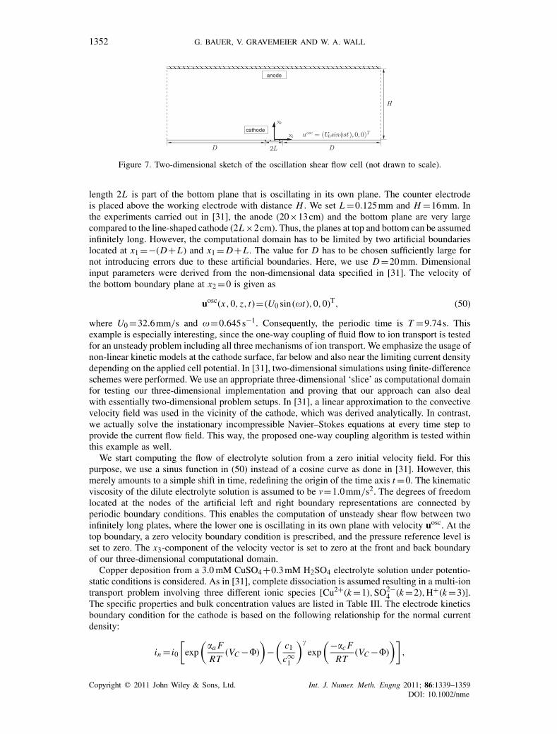
1352 G. BAUER, V. GRAVEMEIER AND W. A. WALL
Figure 7. Two-dimensional sketch of the oscillation shear flow cell (not drawn to scale).
length 2L is part of the bottom plane that is oscillating in its own plane. The counter electrodeis placed above the working electrode with distance H . We set L =0.125mm and H =16mm. Inthe experiments carried out in [31], the anode (20×13cm) and the bottom plane are very largecompared to the line-shaped cathode (2L ×2cm). Thus, the planes at top and bottom can be assumedinfinitely long. However, the computational domain has to be limited by two artificial boundarieslocated at x1 =−(D+L) and x1 = D+L . The value for D has to be chosen sufficiently large fornot introducing errors due to these artificial boundaries. Here, we use D =20mm. Dimensionalinput parameters were derived from the non-dimensional data specified in [31]. The velocity ofthe bottom boundary plane at x2 =0 is given as
uosc(x,0, z, t)= (U0 sin(t),0,0)T, (50)
where U0 =32.6mm/s and =0.645s−1. Consequently, the periodic time is T =9.74s. Thisexample is especially interesting, since the one-way coupling of fluid flow to ion transport is testedfor an unsteady problem including all three mechanisms of ion transport. We emphasize the usage ofnon-linear kinetic models at the cathode surface, far below and also near the limiting current densitydepending on the applied cell potential. In [31], two-dimensional simulations using finite-differenceschemes were performed. We use an appropriate three-dimensional ‘slice’ as computational domainfor testing our three-dimensional implementation and proving that our approach can also dealwith essentially two-dimensional problem setups. In [31], a linear approximation to the convectivevelocity field was used in the vicinity of the cathode, which was derived analytically. In contrast,we actually solve the instationary incompressible Navier–Stokes equations at every time step toprovide the current flow field. This way, the proposed one-way coupling algorithm is tested withinthis example as well.
We start computing the flow of electrolyte solution from a zero initial velocity field. For thispurpose, we use a sinus function in (50) instead of a cosine curve as done in [31]. However, thismerely amounts to a simple shift in time, redefining the origin of the time axis t =0. The kinematicviscosity of the dilute electrolyte solution is assumed to be �=1.0mm/s2. The degrees of freedomlocated at the nodes of the artificial left and right boundary representations are connected byperiodic boundary conditions. This enables the computation of unsteady shear flow between twoinfinitely long plates, where the lower one is oscillating in its own plane with velocity uosc. At thetop boundary, a zero velocity boundary condition is prescribed, and the pressure reference level isset to zero. The x3-component of the velocity vector is set to zero at the front and back boundaryof our three-dimensional computational domain.
Copper deposition from a 3.0 mM CuSO4 +0.3mM H2SO4 electrolyte solution under potentio-static conditions is considered. As in [31], complete dissociation is assumed resulting in a multi-iontransport problem involving three different ionic species [Cu2+(k =1),SO2−
4 (k =2),H+(k =3)].The specific properties and bulk concentration values are listed in Table III. The electrode kineticsboundary condition for the cathode is based on the following relationship for the normal currentdensity:
in = i0
[exp
(�a F
RT(VC −�)
)−
(c1
c∞1
)�
exp
(−�c F
RT(VC −�)
)],
Copyright � 2011 John Wiley & Sons, Ltd. Int. J. Numer. Meth. Engng 2011; 86:1339–1359DOI: 10.1002/nme

3D FINITE ELEMENT APPROACH FOR COUPLED ELECTROCHEMICAL SYSTEMS 1353
Table III. Material parameters and electrolyte bulk concentrations of ionic species.
Ionic species Cu2+ SO2−4 H+
zk +2 −2 +1
Dk ×103mm2/s 0.72 1.065 9.312
c∞k ×1�mol/mm3 0.003 0.103 0.2
with concentration dependency only present at the cathodic term. The parameter values are i0 =−4.0�A/mm2, �=0.5, �a =1.5 and �c =0.5. The anode potential defines the reference level for� and is set to zero (VA =0V ). No overpotential is considered at the anode. The potential VC atthe metal side of the cathode is VC =−0.05V in the first experiment, corresponding to 45% oflimiting current density, and VC =−0.13V in the second one. Following Yang and West [31], thelatter corresponds to 97% of limiting current density. The applied cell potential differences are thesame as those used in the reference, but we use a different reference level for the electric potential.Since the temperature T of the electrolyte solution was not explicitly given in the reference, weassume a reasonable value of T =298K. At left, right and top boundary, being far away from thecathode, we demand ck =c∞
k and �=0. At all other boundary parts not yet discussed, zero massflux is assumed for all concentrations. It is beneficial to solve the electrochemistry equations in aframe of reference where the cathode and its associated boundary part are at rest. Thus, the relativemotion of electrolyte solution with respect to the origin is required for solving the electrochemistryproblem. Consequently, the velocity of the origin has to be subtracted from the velocity field uf
computed from the Navier–Stokes solver. Thus, the relative convective velocity to be used in theion-transport equations reads
u(x, t)=uf(x, t)−uosc(0, t) (51)
being zero all along the bottom boundary plane. Since we consider fluid flow and ionic transportin the complete area between the parallel planes, one can choose H/2 as characteristic length anda time-averaged velocity value of 2U0/ as characteristic velocity. The corresponding Reynoldsnumber is Re=U0 H/�=166 and the according value for the Peclet number reads Pe=Re·Sc=230609 with a Schmidt number of Sc=�/D1 =1389. A particular definition of a Peclet numberwas given in [31], reading Pe= (/�)0.5U0L2/D1 =568.
The computational domain is discretized using a symmetric mesh with 184 elements in thex1-direction and 60 in the x2-direction. The thickness of the slice is chosen to be L/20, discretizedwith one element in the x3-direction. Refinement towards the bottom plane is realized with meshgrading using a bias factor of 1.065. The elements next to the bottom plane exhibit a height ofabout 0.0243 mm. Near the cathode surface an additional local refinement is applied (see Figure 8).Thus, the minimum edge length in the x2-direction of elements adjacent to the cathode is locallyreduced to 3.041�m. In total, the mesh consists of 12 296 hexahedral elements with trilinear shapefunctions and 25 148 nodes. We apply a constant time-step length of �t =T/100 in all simulations.For the start-up phase of each simulation, we apply an appropriate smooth ramp function forchanging VC from zero to its final value within one period of oscillation. With four degrees offreedom per node for the fluid problem (velocity uf, pressure p) and four degrees of freedom pernode for the electrochemistry fields (c1,c2,c3,�), in total, more than 200 000 degrees of freedomhave to be determined within each time step.
At least 15 periodic cycles (1500 time steps) are computed before any data evaluation isperformed. This ensures that initial transients have vanished and the quasi-static periodic solutionhas been reached. Figure 9 depicts the computed copper cation concentration profiles near thecathode for the case VC =−0.245V. Snapshots at four different times are provided that clearlyreveal the influence of the oscillating shear flow on the shape of the concentration boundary layer.The periodic changes in the boundary layer thickness cause the observed oscillatory behavior ofmass flux and current density at the cathode surface. In Figure 10, the temporal evolution of thespatially averaged current density at the cathode surface is shown over two periods of oscillation.
Copyright � 2011 John Wiley & Sons, Ltd. Int. J. Numer. Meth. Engng 2011; 86:1339–1359DOI: 10.1002/nme

1354 G. BAUER, V. GRAVEMEIER AND W. A. WALL
Figure 8. Locally refined mesh near the cathode surface.
Figure 9. Concentration boundary layer of Cu2+ forming near the cathodesurface: snapshots at various times within one oscillation period (T =9.74s):
(a) t =146.1s (=15T ); (b) t =148.5s; (c) t =151.0s; and (d) t =153.4s.
Copyright � 2011 John Wiley & Sons, Ltd. Int. J. Numer. Meth. Engng 2011; 86:1339–1359DOI: 10.1002/nme

3D FINITE ELEMENT APPROACH FOR COUPLED ELECTROCHEMICAL SYSTEMS 1355
Figure 10. Temporal evolution of space-averaged cathodic current density. Comparison of computed resultswith experimental data provided in [31].
Figure 11. Numerical results for the temporal evolution of space-averaged surface concen-tration of Cu2+ ions at the cathode.
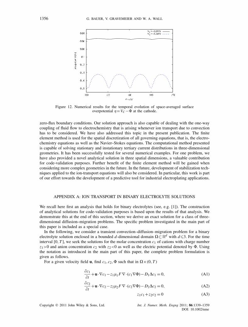
The comparison with the experimental data given in [31] shows excellent agreement for both valuesof applied cell voltages. The computed evolution of copper cation concentration at the cathodesurface relative to the bulk value is depicted in Figure 11. These data are also space-averagedalong the electrode surface. Oscillation of concentration due to periodic shear flow is observedhere as well. For VC =−0.245V the Cu2+-concentration is varying between 1 and 10% of thebulk concentration value reflecting that the cell is operating near the limiting current density inthe second experiment. For the same time interval as before, the average overpotential �=VC −�is finally plotted in Figure 12 for both experiments.
5. CONCLUSIONS
We have presented a new finite element approach to the numerical simulation of electrochem-ical systems. All multi-ion transport phenomena subjected to electroneutrality are addressed inour computational approach. The effects of convection, diffusion, migration as well as the poten-tial use of non-linear phenomenological boundary conditions at electrode surfaces are included.We highlighted the benefit of a convective formulation of ion transport equations for applying
Copyright � 2011 John Wiley & Sons, Ltd. Int. J. Numer. Meth. Engng 2011; 86:1339–1359DOI: 10.1002/nme
1356 G. BAUER, V. GRAVEMEIER AND W. A. WALL
Figure 12. Numerical results for the temporal evolution of space-averaged surfaceoverpotential �=VC −� at the cathode.
zero-flux boundary conditions. Our solution approach is also capable of dealing with the one-waycoupling of fluid flow to electrochemistry that is arising whenever ion transport due to convectionhas to be considered. We have also addressed this topic in the present publication. The finiteelement method is used for the spatial discretization of all governing equations, that is, the electro-chemistry equations as well as the Navier–Stokes equations. The computational method presentedis capable of solving stationary and instationary tertiary current distributions in three-dimensionalgeometries. It has been successfully tested for several numerical examples. For one problem, wehave also provided a novel analytical solution in three spatial dimensions, a valuable contributionfor code-validation purposes. Further benefit of the finite element method will be gained whenconsidering more complex geometries in the future. In the future, development of stabilization tech-niques applied to the ion-transport equations will also be considered. In particular, this work is partof our effort towards the development of a predictive tool for industrial electroplating applications.
APPENDIX A: ION TRANSPORT IN BINARY ELECTROLYTE SOLUTIONS
We recall here first an analysis that holds for binary electrolytes (see, e.g. [1]). The constructionof analytical solutions for code-validation purposes is based upon the results of that analysis. Wedemonstrate this at the end of this section, where we derive an exact solution for a class of three-dimensional diffusion–migration problems. The specific problem investigated in the main part ofthis paper is included as a special case.
In the following, we consider a transient convection–diffusion–migration problem for a binaryelectrolyte solution enclosed in a bounded d-dimensional domain �⊂Rd with d�3. For the timeinterval [0,T ], we seek the solutions for the molar concentration c1 of cations with charge numberz1>0 and anion concentration c2 with z2<0 as well as the electric potential denoted by �. Usingthe notation as introduced in the main part of this paper, the complete problem formulation isgiven as follows.
For a given velocity field u, find c1,c2,� such that in �×(0,T )
�c1
�t+u·∇c1 −z1�1 F ∇ ·(c1∇�)− D1�c1 = 0, (A1)
�c2
�t+u·∇c2 −z2�2 F ∇ ·(c2∇�)− D2�c2 = 0, (A2)
z1c1 +z2c2 = 0 (A3)
Copyright � 2011 John Wiley & Sons, Ltd. Int. J. Numer. Meth. Engng 2011; 86:1339–1359DOI: 10.1002/nme

3D FINITE ELEMENT APPROACH FOR COUPLED ELECTROCHEMICAL SYSTEMS 1357
together with boundary and initial conditions for k =1,2:
ck = gk on �D,k ×(0,T ), (A4)
(zk�k Fck∇�+ Dk∇ck) ·n = hk on �N,k ×(0,T ), (A5)
ck = c0k in �×{0}, (A6)
ck > 0 in �×[0,T ]. (A7)
Owing to the electroneutrality condition (A3), the anion concentration c2 is already uniquelydetermined by c1 via
c2 =− z1
z2c1. (A8)
Consequently, we require c02 = (−z1/z2)c0
1 to be satisfied by the initial conditions. Furthermore, c2can be eliminated from (A2) by multiplication with −z2/z1 and application of (A8). Subtractionof the resulting equation from (A1) then yields:
(z2�2 −z1�1)F ∇ ·(c1∇�)+(D2 − D1)�c1 =0. (A9)
From the expression for the current density
i= F2∑
k=1zk(−Dk∇ck −zk�k Fck∇�) (A10)
as introduced in (16), the following integrated form of (A9) is deduced by using (A8):
iz1 F
= (z2�2 −z1�1)Fc1∇�+(D2 − D1)∇c1. (A11)
For problems where no current i is passing the electrochemical cell, a solution formula for theelectric potential � can be deduced by integration, which is applicable once c1 is known:
�(x, t)−�(x0, t)= D2 − D1
(z1�1 −z2�2)Fln
(c1(x, t)
c1(x0, t)
). (A12)
Here, x0 ∈� is an arbitrary point with c1(x0, t)>0∀t ∈ [0,T ]. Finally, using (A9) in (A1) revealsthat the concentration c1 is governed by a transient convection–diffusion equation of the form
�c1
�t+u·∇c1 − D�c1 =0 in �×(0,T ) (A13)
with a resulting diffusion coefficient
D := z1�1 D2 −z2�2 D1
z1�1 −z2�2(A14)
depending on the properties of both ionic species of interest. In the same manner as before, we caneliminate c2 and � from the flux boundary conditions (A5), resulting in a new boundary condition
D∇c1 ·n=h∗ on �N,1 ×(0,T ) (A15)
with
h∗ := (−z2)(�2h1 +�1h2)
z1�1 −z2�2,
which has to be fulfilled by the solution of (A13). In summary, the task of solving the coupled non-linear ion-transport problem (A1)–(A7) has been reduced to solving a linear convection–diffusionproblem for c1 governed by Equation (A13) with boundary conditions (A4) and (A15) and initial
Copyright � 2011 John Wiley & Sons, Ltd. Int. J. Numer. Meth. Engng 2011; 86:1339–1359DOI: 10.1002/nme

1358 G. BAUER, V. GRAVEMEIER AND W. A. WALL
condition (A6). The analysis shown above holds for an arbitrary number of space dimensionsand is the basis for the construction of analytical solutions for ion-transport problems in binaryelectrolyte solutions.
For deducing the analytical solution of the diffusion–migration problem investigated inSection 4.1, set u=0, and h1 =h2 =0 on �N,1 =�N,2 =��. Let the initial condition c0
1 for thecation concentration c1 be given in the following form:
c01(x, y, z)= A0 +
L∑l=1
M∑m=1
N∑n=1
flmn(x, y, z) in �
with flmn(x, y, z) := Almn cos(lx)cos(my)cos(nz). Here, A0, Almn ∈R are arbitrary coeffi-cients and L , M, N ∈N are positive integers. However, the coefficients have to be chosen in sucha way that c0
1(x, y, z)>0 ∀(x, y, z)∈� is ensured. The initial field of c2 is fixed due to electroneu-trality in the form c0
2 =− z1z2
c01. The analytical solution of (A13) is derived using standard solution
techniques for the instationary diffusion equation and reads
c1(x, y, z, t)= A0 +L∑
l=1
M∑m=1
N∑n=1
flmn(x, y, z)e−D(l2+m2+n2)2t .
Since the current density i equals zero due to the homogeneous flux boundary conditions, formula(A12) is applicable specifying the electric potential. Together with (A8), the analytical solutionfor the diffusion–migration problem with the given specifications has been derived. To obtain thesolution formulae specified in Section 4.1, we just have to set A0 =2 and A123 =1, while all otherAlmn equal zero.
ACKNOWLEDGEMENTS
The financial support by the Space Agency of the German Aerospace Center (DLR) under grant 50RL0743is gratefully acknowledged. The support of the second author via the Emmy Noether program of theDeutsche Forschungsgemeinschaft (DFG) is also gratefully acknowledged.
REFERENCES
1. Newman J, Thomas-Alyea KE. Electrochemical Systems (3rd edn). Wiley: New York, 2004.2. He X, Li N. Lattice Boltzmann simulation of electrochemical systems. Computer Physics Communications 2000;
129:158–166.3. La Rocca A, Power H. Free mesh radial basis function collocation approach for the numerical solution of system
of multi-ion electrolytes. International Journal for Numerical Methods in Engineering 2005; 64:1699–1734.4. Georgiadou M. Finite-difference simulation of multi-ion electrochemical systems governed by diffusion, migration
and convection. Journal of The Electrochemical Society 1997; 144:2732–2739.5. Georgiadou M. Modeling current density distribution in electrochemical systems. Electrochimica Acta 2003;
48:4089–4095.6. Georgiadou M, Mohr R, Alkire RC. Local mass transport in two-dimensional cavities in laminar shear flow.
Journal of The Electrochemical Society 2000; 147:3021–3028.7. Bortels L, Deconinck J, Van den Bossche B. The multi-dimensional upwinding method as a new simulation tool
for the analysis of multi-ion electrolytes controlled by diffusion, convection and migration. Part 1. Steady stateanalysis of a parallel plane flow channel. Journal of Electroanalytical Chemistry 1996; 404:15–26.
8. Buoni M, Petzold L. An efficient, scalable numerical algorithm for the simulation of electrochemical systems onirregular domains. Journal of Computational Physics 2007; 225:2320–2332.
9. Buoni M, Petzold L. An algorithm for simulation of electrochemical systems with surface-bulk coupling strategies.Journal of Computational Physics 2010; 229:379–398.
10. Kwok YK, Wu CCK. Fractional step algorithm for solving a multi-dimensional diffusion–migration equation.Numerical Methods for Partial Differential Equations 1995; 11:389–397.
11. Barak-Shinar D, Rosenfeld M, Abboud S. Numerical simulations of mass-transfer processes in 3D model ofelectrochemical sensor. Journal of The Electrochemical Society 2004; 151:H261–H266.
12. Henley IE, Fisher AC. Computational electrochemistry: The simulation of voltammetry in microchannels withlow conductivity solutions. The Journal of Physical Chemistry B 2003; 107:6579–6585.
13. Samson E, Marchand J, Robert JL, Bournazel JP. Modelling ion diffusion mechanisms in porous media.International Journal for Numerical Methods in Engineering 1999; 46:2043–2060.
Copyright � 2011 John Wiley & Sons, Ltd. Int. J. Numer. Meth. Engng 2011; 86:1339–1359DOI: 10.1002/nme

3D FINITE ELEMENT APPROACH FOR COUPLED ELECTROCHEMICAL SYSTEMS 1359
14. Lee J, Talbot JB. A model of electrocodeposition on a rotating cylinder electrode. Journal of The ElectrochemicalSociety 2007; 154:D70–D77.
15. Ludwig K, Morales I, Speiser B. Echem++—an object-oriented problem solving environment for electrochemistryPart 6. Adaptive finite element simulations of controlled-current electrochemical experiments. Journal ofElectroanalytical Chemistry 2007; 608:102–110.
16. Ganjoo DK, Tezduyar TE. Petrov-Galerkin formulations for electrochemical processes. Computer Methods inApplied Mechanics and Engineering 1987; 65(1):61–83.
17. Lin PT, Shadid JN, Sala M, Tuminaro RS, Hennigan GL, Hoekstra RJ. Performance of a parallel algebraicmultilevel preconditioner for stabilized finite element semiconductor device modeling. Journal of ComputationalPhysics 2009; 228:6250–6267.
18. Gravemeier V, Wall WA. A ‘divide-and-conquer’ spatial and temporal multiscale method for transient convection–diffusion–reaction equations. International Journal for Numerical Methods in Fluids 2007; 54:779–804.
19. Gravemeier V, Wall WA, Ramm E. A three-level finite element method for the instationary incompressibleNavier–Stokes equations. Computer Methods in Applied Mechanics and Engineering 2004; 193:1323–1366.
20. Gravemeier V, Lenz S, Wall WA. Variational multiscale methods for incompressible flows. International Journalof Computing Science and Mathematics 2007; 41:444–466.
21. Gravemeier V, Gee MW, Kronbichler M, Wall WA. An algebraic variational multiscale-multigrid method forlarge eddy simulation of turbulent flow. Computer Methods in Applied Mechanics and Engineering 2010;199(13–16):853–864.
22. Gravemeier V, Wall WA. Residual-based variational multiscale methods for laminar, transitional and turbulentvariable-density flow at low Mach number. International Journal for Numerical Methods in Fluids, in press,available online. DOI: 10.1002/fld.2242.
23. Gravemeier V, Wall WA. An algebraic variational multiscale-multigrid method for large-eddy simulation ofturbulent variable-density flow at low Mach number. Journal of Computational Physics 2010; 229(17):6047–6070.
24. Hughes T, Scovazzi G, Franca L. Multiscale and stabilized methods. In Encyclopedia of Computational Mechanics,Stein E, de Borst R, Hughes T (eds). Wiley: Chichester, 2004; 5–59.
25. Davis TA. Algorithm 832: Umfpack v4.3—an unsymmetric-pattern multifrontal method. ACM Transactions onMathematical Software 2004; 30:196–199.
26. Benzi M, Golub GH, Liesen J. Numerical solution of saddle point problems. Acta Numerica 2005; 14:1–137.27. Gerstenberger A, Wall WA. An extended finite element method/Lagrange multiplier based approach for fluid–
structure interaction. Computer Methods in Applied Mechanics and Engineering 2008; 197:1699–1714.28. Gerstenberger A, Wall WA. An embedded Dirichlet formulation for 3D continua. International Journal for
Numerical Methods in Engineering 2010; 82(5):537–563.29. Choi YS, Chan KY. Exact solutions of transport in a binary electrolyte. Journal of Electroanalytical Chemistry
1992; 334:13–23.30. Choi YS, Yu X. Steady-state solution for electroplating. IMA Journal of Applied Mathematics 1993; 51:251–267.31. Yang JD, West AC. Current distributions governed by coupled concentration and potential fields. AIChE Journal
1997; 43:811–817.
Copyright � 2011 John Wiley & Sons, Ltd. Int. J. Numer. Meth. Engng 2011; 86:1339–1359DOI: 10.1002/nme


![����-��Q�kTitle ����-��Q�k Author ï¿½ï¿½ï¿½Ý t�]�c Created Date �����-�](https://img.dokumen.tips/doc/110x75/60a3a35fc4ece70e851f9842/-qk-title-qk.jpg)