Embed Size (px)
Citation preview

University of New MexicoUNM Digital Repository
Mechanical Engineering ETDs Engineering ETDs
1-28-2015
A 3D Computational Fluid Dynamics ModelValidation for Candidate Molybdenum-99 TargetGeometryLin Zheng
Follow this and additional works at: https://digitalrepository.unm.edu/me_etds
This Thesis is brought to you for free and open access by the Engineering ETDs at UNM Digital Repository. It has been accepted for inclusion inMechanical Engineering ETDs by an authorized administrator of UNM Digital Repository. For more information, please contact [email protected].
Recommended CitationZheng, Lin. "A 3D Computational Fluid Dynamics Model Validation for Candidate Molybdenum-99 Target Geometry." (2015).https://digitalrepository.unm.edu/me_etds/89

i
Lin Zheng Candidate
Mechanical Engineering
Department
This thesis is approved, and it is acceptable in quality and form for publication:
Approved by the Thesis Committee:
Peter Vorobieff, Chairperson
Svetlana Poroseva
Eric Olivas

ii
A 3D Computational Fluid Dynamics Model Validation for
Candidate Molybdenum-99 Target Geometry
By
LIN ZHENG
B.S MECHANICAL ENGINEERING, UNIVERSITY OF NEW
MEXICO (2012)
THESIS
Submitted in Partial Fulfillment of the
Requirements for the Degree of
Master of Science
Mechanical Engineering
The University of New Mexico
Albuquerque, New Mexico
December 2014

iii
Acknowledgements
First, I would like to thank Dr. Greg Dale, of Los Alamos National Laboratory,
for providing this project. He provided me the history and background of this project.
He helped me understand how significant this project will benefit our society. Several
other individuals that I’d also like to thank for and they are:
Dr. Peter Vorobieff, my advisor and professor at the University of New Mexico,
for providing guidance and direction when it was needed at any time. He encouraged me
to record all my research progress by constructing a series of bi-weekly progress reports.
It had really helped me on the development of this thesis.
Keith Woloshun, Frank Romero, and Eric Olivas, of Los Alamos National
Laboratory, for their supports and helps on both model and experiment developments for
this project.
Nima Fathi, PhD Candidate at the University of New Mexico, for explaining me
the process of doing computational fluid dynamics modeling. He provided me ideas of
how to do verification and validation for my CFD model.
Donald Mercer and Sloan Pearsall, my office mates at the University of New
Mexico, for proving me help in different academic areas. I have to thank them for spent
those long hours in the office with me to develop this thesis.

iv
A 3D COMPUTATIONAL FLUID DYNAMICS MODEL VALIDATION FOR CANDIDATE
MOLYBDENUM-99 TARGET GEOMETRY
By
Lin Zheng
B.S. Mechanical Engineering, University of New Mexico, 2012
M.S. Mechanical Engineering, University of New Mexico, 2014
Abstract
As part of its nuclear nonproliferation mission, the U.S. Department of Energy’s
Global Threat Reduction Initiative (GTRI) is working to develop a sustainable means for
producing the critical medical isotope molybdenum-99 (99
Mo) without using highly
enriched uranium (HEU). 99
Mo is the parent product of technetium99m (99m
Tc), a
radioisotope used in approximately 50,000 medical diagnostic tests per day in the U.S.
The primary uses of this product include detection of heart disease, cancer, study of organ
structure and function, and other applications. 99
Mo has a short half-life (66 hours) and
cannot be stockpiled. U.S. demand is approximately 50% of the world market. The
objective of the domestic 99
Mo project is to accelerate existing commercial projects to
meet at least 100% of the U.S. demand of 99
Mo produced without HEU by the end of
2016.
New methods for generating 99
Mo are being explored in an effort to eliminate
proliferation issues and provide a domestic supply of 99m
Tc for medical imaging within

v
the United States. For this project, electron accelerating technology is used by sending an
electron beam through a series of 100
Mo targets. During this process a large amount of
heat is created, which directly affects the operating temperature set for the system. The
wall temperature along the target section must be maintained between 550 and 650 .
This temperature range is dictated by the tensile stress limit of the wall material.
To maintain the required temperature range, helium gas is used to server as a
cooling agent that flows through narrow channels between the target disks.
This thesis investigated the cooling performance on a series of new geometry
designs of the cooling channel by using Computational Fluid Dynamics (CFD) software
ANSYS FLUENT 14.5. An experiment was also conducted to conclude whether the CFD
model is valid and able to predict the right physics of the cooling channels. As a result, a
new optimal geometry for the cooling channels will be selected for the purpose of the
99Mo project.

vi
Table of Contents
Acknowledgements .......................................................................................................... iii
Abstract ............................................................................................................................. iv
Table of Contents ............................................................................................................. vi
List of Figures ................................................................................................................. viii
List of Tables .................................................................................................................... xi
List of Variables .............................................................................................................. xii
Chapter 1 - Introduction and Literature Review .......................................................... 1
1.1 HISTORY OF 99M
TC PRODUCTION AND USAGE .............................................................................................. 3
1.1.1 Nuclear Medicine Techniques and Development ......................................................................... 4
1.1.2 Early Productions of 99
Mo/99m
Tc ................................................................................................... 4
1.1.3 Highly Enriched Uranium (HEU) Method ...................................................................................... 5
1.1.4 Low Enriched Uranium (LEU) ........................................................................................................ 6
1.1.5 Neutron Activation ....................................................................................................................... 6
1.1.6 Photon Induced Reaction 100
Mo( 99
Mo in Accelerator .......................................................... 6
1.1.7 Overview of Non-HEU processes .................................................................................................. 7
1.2 OVERVIEW OF PROPOSED METHOD ............................................................................................................... 8
1.3 TARGET COOLING SYSTEM ........................................................................................................................... 8
1.3.1 Cooling Fluid Selection .................................................................................................................. 9
1.3.2 Once-through Cooling System .................................................................................................... 10
1.3.3 Closed Loop Helium Gas Cooling System .................................................................................... 11
1.3.4 Flow Properties ........................................................................................................................... 15
Chapter 2 - Theory and Methodology ........................................................................... 17
2.1 MACH NUMBER CALCULATION ................................................................................................................... 17
2.2 DENSITY CALCULATION ............................................................................................................................. 18
2.3 CONFINED FLOWS .................................................................................................................................... 18
2.4 REYNOLDS NUMBER ................................................................................................................................. 19
2.5 CFD MODELS ......................................................................................................................................... 20
2.5.1 Turbulence Models ..................................................................................................................... 21
Chapter 3 - CFD Model Development .......................................................................... 29

vii
3.1 GEOMETRY ............................................................................................................................................. 30
3.2 SINGLE CHANNEL MODEL .......................................................................................................................... 32
3.2.1 Turbulence Model Validation ..................................................................................................... 34
3.2.2 Boundary Conditions and Model Inputs ..................................................................................... 36
3.2.3 Mesh Development .................................................................................................................... 38
3.2.4 Result Monitoring ....................................................................................................................... 46
3.3 MULTI-CHANNELS MODEL ........................................................................................................................ 49
3.3.1 Multi-Channels Boundary Conditions and Model Inputs ............................................................ 49
3.3.2 Multi-Channels Mesh Development ........................................................................................... 51
Chapter 4 – Design Decision and Model Reduction .................................................... 58
4.1 INLET FEATURE SELECTION ......................................................................................................................... 58
4.2 SINGLE CHANNEL DIFFUSER ANGLE SELECTION .............................................................................................. 63
4.3 MULTI-CHANNELS STUDY .......................................................................................................................... 68
4.3.1 Model Reduction for Multi-Channels Study ............................................................................... 68
Chapter 5 – Validation Analysis .................................................................................... 76
5.1 EXPERIMENT SETUP .................................................................................................................................. 76
5.2 EXPERIMENTAL INCIDENCE ......................................................................................................................... 80
5.3 EXPERIMENTAL RESULT ............................................................................................................................. 81
5.4 RESULT AND DISCUSSION .......................................................................................................................... 85
Chapter 6 – Conclusions and Recommendations......................................................... 96
6.1 CONCLUSIONS ......................................................................................................................................... 96
6.2 SUGGESTIONS FOR FUTURE WORK .............................................................................................................. 98
References ...................................................................................................................... 100

viii
List of Figures
Figure 1.1: GTRI and U.S Domestic Mo-99: Non-HEU Production Methods................................................ 7
Figure 1.2: Photograph of the Helium Gas Bottle and Gas Manifold Used During the Once-through Helium
Gas Cooled Thermal Test Using the Electron Accelerator at ANL in March 2011 ...................................... 11
Figure 1.3: Photograph of the Roots Blower (Left) and Motor (Right) Mounted to a Plate Cantileverd of the
End of the Pressure Vessle Flange Plate. The Other End of the Pressure Vessel Slides Back and Forth Over
the Motor and Blower on Rails Bolted to the Skid Plate ............................................................................... 13
Figure 1.4: P&ID of the Production System.................................................................................................. 14
Figure 1.5: Piping Layout for the Helium Target Cooling System................................................................ 15
Figure 3.1: Exploded ISO view of housing, holder, and targets. Tubes that are located at the holder chimney
flange are for thermocouple insertion. ........................................................................................................... 30
Figure 3.2: Cross-section view of Mo99 Target and Vacuum Cube Assembly showing assembly and weld
locations. ....................................................................................................................................................... 31
Figure 3.3: Target Disks and Production Configuration ............................................................................... 32
Figure 3.4: Original Target Cooling Channel (Single Channel Base Case) .................................................. 33
Figure 3.5: Obi's Diffuser Geometry ............................................................................................................. 34
Figure 3.6: Development of axial velocity profile through the diffuser for the tested turbulence models
compared with an experimental result of Buice-Eaton data. [19] ................................................................. 35
Figure 3.7: Mean Stream Velocity Comparison in a 10-Degree Diffuser (Model Validation) ..................... 36
Figure 3.8: Single Channel Components ....................................................................................................... 37
Figure 3.9: A Typical Mesh Used in the Calculation - Quarter Circle Inlet (438,216 Nodes) ...................... 38
Figure 3.10: A Typical Mesh Used in the Calculation - Diffuser Outlet (438,216 Nodes) ........................... 38
Figure 3.11: Mesh Study – Mid-section Velocity Profile Comparison SKW Model .................................... 42
Figure 3.12: Mesh Study – Mid-section Velocity Profile Comparison SSTKW Model ............................... 42
Figure 3.13: Mesh Configuration - 59,136 Nodes Inlet ................................................................................. 43
Figure 3.14: Mesh Configuration - 438,216 Nodes Inlet ............................................................................... 43
Figure 3.15: Mesh Configuration - 788,020 Nodes Inlet ............................................................................... 43
Figure 3.16: Mesh Configuration – 59,136 Nodes Outlet ............................................................................. 44
Figure 3.17: Mesh Configuration - 438,216 Nodes Outlet ............................................................................ 44
Figure 3.18: Mesh Configuration - 788,020 Nodes Outlet ............................................................................ 44
Figure 3.19: Mesh Configuration - 59,136 Nodes ISO View ........................................................................ 45
Figure 3.20: Mesh Configuration - 438,216 Nodes ISO View ...................................................................... 45
Figure 3.21: Mesh Configuration - 788,020 Nodes ISO View ...................................................................... 46
Figure 3.22: Scaled Residuals - Single Channel ............................................................................................ 47
Figure 3.23: Mass Flow Rate @ Outlet - Single Channel ............................................................................. 48

ix
Figure 3.24: Dynamic Pressure @ Inlet - Single Channel ............................................................................. 48
Figure 3.25: Multi-Channels Components .................................................................................................... 50
Figure 3.26: Quarter Circle Inlet (2,392,054 Nodes Velocity Contour) - Multi-Channels ............................ 51
Figure 3.27: Diffuser Outlet (2,392,054 Nodes Velocity Contour) - Multi-Channels ................................... 52
Figure 3.28: Diffuser Outlet (2,392,054 Nodes Velocity Contour) - Close Up ............................................. 52
Figure 3.29: Scaled Residuals – Multi-Channels (1,594,242 nodes) SSTKW .............................................. 54
Figure 3.30: Scaled Residuals – Multi-Channels (2,392,054 nodes) SSTKW .............................................. 54
Figure 3.31: Scaled Residuals - Multi-Channels (3,276,750 nodes) SSTKW ............................................... 55
Figure 3.32: Inlet Dynamic Pressure - Multi-Channels (1,594,242 nodes) SSTKW ..................................... 55
Figure 3.33: Inlet Dynamic Pressure - Multi-Channels (2,392,054 nodes) SSTKW ..................................... 56
Figure 3.34: Inlet Dynamic Pressure - Multi-Channels (3,276,750 nodes) SSTKW ..................................... 56
Figure 3.35: 2,392,054 Nodes Mesh - Velocity Contour .............................................................................. 57
Figure 4.1: Quarter Circle Inlet ..................................................................................................................... 59
Figure 4.2: 45° Angled Inlet .......................................................................................................................... 59
Figure 4.3: Sudden Expansion Outlet ............................................................................................................ 59
Figure 4.4: Steady State Velocity Contour for Quarter Circle Inlet - SSTKW ............................................. 60
Figure 4.5: Steady State Velocity Contour for 45 Degree Angled Inlet - SSTKW ....................................... 60
Figure 4.6: Steady State Velocity Streamline for Sudden Contraction Inlet - SSTKW ................................ 60
Figure 4.7: Steady State Velocity Streamline for Quarter Circle Inlet - SSTKW ......................................... 61
Figure 4.8: Steady State Velocity Streamline for 45 Degree Angled Inlet - SSTKW ................................... 61
Figure 4.9: SKW Model - Streamline Paths and Velocity Magnitude with Different Diffuser Angles: (a)
,(b) , (c) , (d) , (e) , (f) , (g) , and (h) ............. 64
Figure 4.10: SSTKW Model Streamline Paths and Velocity Magnitude with Different Diffuser Angles: (a)
,(b) , (c) , (d) , (e) , (f) , (g) , and (h) ............. 65
Figure 4.11: Diffuser Angle vs. Mass Flow .................................................................................................. 67
Figure 4.12: Full Model Mesh (27 Channels with 4 Degree Diffuser) .......................................................... 69
Figure 4.13: Full Model Velocity Streamline (27 Channels with 4 Degree Diffuser – SSTKW Model) ...... 70
Figure 4.14: 1/10 Model Velocity Streamline (27 Channels with 4 Degree Diffuser – SSTKW Model) ..... 71
Figure 4.15: 1/10 Model Convergence History - Inlet Dynamic Pressure (SKW) ........................................ 72
Figure 4.16: 1/10 Model Convergence History - Inlet Dynamic Pressure (SSTKW) ................................... 72
Figure 4.17: 1/10 Model Convergence History - Inlet Velocity Magnitude (SKW) ..................................... 73
Figure 4.18: 1/10 Model Convergence History - Inlet Velocity Magnitude (SSTKW) ................................. 73
Figure 4.19: 1/10 Model Convergence History - Inlet Mass Flow Rate (SKW) ........................................... 74
Figure 4.20: 1/10 Model Convergence History - Inlet Mass Flow Rate (SSTKW) ....................................... 74
Figure 5.1: A Typical Design Drawing for Mo99 Project ............................................................................. 77
Figure 5.2: Mo99 Target Prototype Front ..................................................................................................... 77
Figure 5.3: Mo99 Target Prototype Side View ............................................................................................. 78

x
Figure 5.4: Solidworks Model for Test Section ............................................................................................ 78
Figure 5.5: Experiment Instruments Setup .................................................................................................... 79
Figure 5.6: Experiment Target Placement ..................................................................................................... 79
Figure 5.7: Experiment Incidence - Two Collapsed Disks ............................................................................ 80
Figure 5.8: Experiment Incidence – Broken Disks ........................................................................................ 81
Figure 5.9: Experimental Result - Pressure Drop vs. Mass Flow .................................................................. 82
Figure 5.10: Diffuser Angle vs. Mass Flow – Experimental Data (@15 Psi) ............................................... 84
Figure 5.11: Velocity Streamline - Sudden Contraction and Expansion (SSTKW Model) ........................... 86
Figure 5.12: Velocity Streamline - Sudden Contraction and Expansion (SKW Model) ............................... 86
Figure 5.13: Velocity Streamline - Quarter Circle Inlet (SSTKW Model) .................................................... 87
Figure 5.14: Velocity Streamline - Quarter Circle Inlet (SKW Model) ........................................................ 87
Figure 5.15: Velocity Streamline - 3 Degree Diffuser (SSTKW Model) ...................................................... 88
Figure 5.16: Velocity Streamline - 3 Degree Diffuser (SKW Model) ........................................................... 88
Figure 5.17: Velocity Streamline - 4 Degree Diffuser (SSTKW Model) ...................................................... 89
Figure 5.18: Velocity Streamline - 4 Degree Diffuser (SKW Model) ........................................................... 89
Figure 5.19: Velocity Streamline - 5 Degree Diffuser (SSTKW Model) ...................................................... 90
Figure 5.20: Velocity Streamline - 5 Degree Diffuser (SKW Model) ........................................................... 90
Figure 5.21: Velocity Streamline - 6 Degree Diffuser (SSTKW Model) ...................................................... 91
Figure 5.22: Velocity Streamline - 6 Degree Diffuser (SKW Model) ........................................................... 91
Figure 5.23: Final Result Comparison – Models vs. Experimental Data ...................................................... 93
Figure 5.24: Mass Flow as a Function of Pressure Drop ............................................................................... 94

xi
List of Tables
Table 1.1: Main Mo-99 Production Reactors .................................................................................................. 2
Table 1.2: Gas Coolant Properties ................................................................................................................... 9
Table 2.1: Standard k- Model Closure Coefficients Comparison ............................................................... 26
Table 2.2: SST k- Model Closure Coefficients Comparison ...................................................................... 28
Table 3.1: Mesh Skewness ............................................................................................................................ 41
Table 3.2: Single Channel Mesh Metrics ...................................................................................................... 41
Table 3.3: Multi-Channels Mesh Matrix (3 Degree Diffuser) ....................................................................... 53
Table 4.1: Inlet Geometries Performance Comparison (Single Channel SKW Model) ................................ 62
Table 4.2: Inlet Geometries Performance Comparison (Single Channel SSTKW Model) ............................ 63
Table 4.3: Parametric Study: Single Channel ................................................................................................ 65
Table 4.4: Mass Flow Improvement for Different Diffusers ......................................................................... 67
Table 4.5: Full Model Mesh Matrix .............................................................................................................. 69
Table 4.6: 1/10 Model Mesh Matrix .............................................................................................................. 71
Table 5.1: Pressure Drop vs. Mass Flow – Geometry Comparison ............................................................... 83
Table 5.2: Mass Flow Percentage Improvement ........................................................................................... 83
Table 5.3: Results Comparison - Models vs. Experimental Data (@15 Psi Pressure Drop) ......................... 92

xii
List of Variables
Power
Mass flow rate
Average outlet temperature
Average inlet temperature
Mach number
Velocity
Speed of sound
Density
Bulk modulus of elasticity
Thermal conductivity
Gas constant
Absolute temperature
Pressure
Volumetric flow rate
Area
Reynolds number
Characteristic length
Dynamic viscosity
Turbulence viscosity
Directional velocity components
Average fluctuating velocity component
1
Chapter 1 - Introduction and Literature Review
Nuclear Medicine is a branch of medicine that uses radiation to provide
information about the functioning of a person’s specific organs or to treat disease. Over
10,000 hospitals worldwide use radioisotopes in medicine and about 90% of the
procedures are for diagnostics. The most common radioisotope used in diagnosis is
technetium99m (99m
Tc), with some 40 million procedures per year (16.7 million in USA
in 2012), accounting for 80% of all nuclear medicine procedures worldwide. [1]
One of reasons that 99m
Tc is so popular in the nuclear medicine world is because
of its short half-life. It has a half-life of six hours which is long enough to examine
metabolic process yet short enough to minimize the radiation dose to the patient.
However, the short half-life of 99m
Tc radioisotopes has created an issue when transporting
them from the facility where they are created to their end users. To resolve this issue,
99mTc must be transported in the form of molybdenum-99 (
99Mo), which is the parent
isotope of 99m
Tc. 99
Mo has a longer half-life of 66 hours and cannot be stockpiled.
Over 99% of the 99
Mo is made in five reactors: NRU in Canada (40%), HFR in
Netherlands (30%), BR-2 in Belgium (9%), Osiris in France (5%), and Safari-1 in South
Africa (10%). [1] Table 1.1 shows more info on the current 99
Mo production reactors.
In addition to the information provided above, statistics show that the entire U.S.
supply of 99
Mo for nuclear medicine has been produced in aging foreign reactors using
highly enriched uranium (HEU) targets. Within the last few years, maintenance and

2
repair shutdowns of these reactors have significantly disrupted the supply of 99
Mo in the
U.S. and much of the rest of the world. [2]
Table 1.1: Main Mo-99 Production Reactors
Because of the issues described above, Los Alamos National Laboratory (LANL)
and Argonne National Laboratory (ANL) are working together with NorthStar Medical
Technologies, LLC as part of the National Nuclear Security Administration (NSSA)
Global Threat Reduction Initiative’s (GTRI) program to accelerate the establishment of a
reliable domestic supply of 99
Mo for nuclear medicine, produced without the use of HEU
targets. [2]
Experiments are being performed by LANL and ANL to develop and demonstrate
the technology necessary for large scale production of 99
Mo using high-power electron
accelerators. 99
Mo is produced with electron accelerators using the 100
Mo( 99Mo
reaction in an enriched 100
Mo target. This reaction has a threshold of 9 MeV and peak
cross section of 150 mb. The photons for this reaction are generated by bremsstrahlung as
Reactor Targets Capacity* Start Est Stop
Belgium BR-2 HEU 289 1961 2026
Netherlands HFR HEU 173 1961 2022
Czech Rep LVR-5 HEU 104 1989 2028
Poland Maria LEU 71 1974 2030
Canada NRU HEU 173 1957 2016
Australia OPAL LEU 37 2006 2030+
France OSIRIS HEU 44 1966 2015+
Argentina RA-3 LEU 15 1967 2027
Russia RIAR HEU 33 1961-70 --
South Africa Safari-1 LEU 111 1965 2025
Total -- -- 1050 -- --

3
the electron beam from the accelerator collides with the target. After irradiation, the low
specific activity 99
Mo is separated from the target using a two column generator
developed by NorthStar Medical Technologies, LLC. [2] [3]
The subject currently under investigation in this work is mainly focused on the
target cooling. The relationship between the behavior of the cooling fluid and the channel
geometries are studied. The result of this thesis will provide a series of data (velocity,
mass flow rate, and pressure drop, etc.) and comparisons to come up with a new design to
optimize the heat transfer ability of the system.
1.1 History of 99m
Tc Production and Usage
99mTc was the first artificially produced element.
99mTc also occurs naturally in
very small amount in the earth’s crust. It was discovered by Carol Perrier and Emilio
Segre in 1937. 99m
Tc was created by bombarding molybdenum atoms with deuterons that
had been accelerated by a device called a cyclotron at University of California, Berkeley.
[4] 99m
Tc was first obtained from molybdenum but is also produced as a nuclear reactor
fission product of uranium and plutonium. All isotopes of technetium are radioactive, and
the most commonly available forms are Tc-99 and Tc-99m. [5]
99mTc is an excellent superconductor at very low temperatures. In addition,
99mTc
has anti-corrosive properties. Five parts of technetium per million will protect carbon
steels from corrosion at room temperature. [5] However, 99m
Tc is primarily used in
medical therapy in brain, bone, liver, spleen, kidney, and thyroid scanning and for blood
flow studies. 99m
Tc is the radioisotope mostly widely used as a tracer for medical
diagnosis. [5]

4
1.1.1 Nuclear Medicine Techniques and Development
As a popular source of nuclear medical imaging, 99m
Tc has played an important
role in the nuclear medicine development. Nuclear medicine was developed in the 1950s
by physicians with an endocrine emphasis, initially using iodine-131 to diagnose and then
treat thyroid disease. In recent years, specialists have also come from radiology, as dual
Computed X-ray Tomography (CT)/Positron Emission Tomography (PET) procedures
have become established. [1]
CT scans and nuclear medicine contribute 36% of the total radiation exposure
and 75% of the medical exposure to the US population, according to a US National
Council on Radiation Protection & Measurement report in 2009. [1]
New procedures combine CT and PET scans to give co-registration of two images
(PETCT), enabling 30% better diagnosis than with traditional gamma camera alone. It is
a very powerful and significant tool which provides unique information on a wide variety
of diseases from dementia to cardiovascular disease and cancer (oncology). [1]
1.1.2 Early Productions of 99
Mo/99m
Tc
Brookhaven reactor pioneered research using subatomic particles as tools to
investigate the structure of matter. The Brookhaven High Flux Beam Reactor first
achieved a self-sustaining chain reaction on October 31, 1965. For over 30 years, this
reactor was one of two premier beam reactors in the world, the other being the Institut
Laue-Langevin reactor in Grenoble, France. [6]

5
The raw material, which is produced in a nuclear reactor, is then transferred to a
processing facility where it is purified through a multi-step process. The finished raw of
99Mo is sent to generator manufactures to introduce them in medical markets for use of its
decay product 99m
Tc in medical applications. In 1959 the U.S. Brookhaven National
Laboratory (BNL) started to develop a generator to produce 99m
Tc from the reactor
fissionable product 99
Mo, which has much longer half-life. The first 99m
Tc radiotracers
were developed at the University of Chicago in 1964. Between 1963 and 1966, the
interest in 99m
Tc grew as its numerous applications, as a radiotracer and diagnostic tool.
By 1966, BNL was unable to cope with the demand for 99
Mo/99m
Tc generators and
withdrew from production and distribution, in favor of commercial generators. [6]
1.1.3 Highly Enriched Uranium (HEU) Method
HEU is the most popular method in the current 99
Mo production system. HEU
includes enough 235
U to maintain a chain reaction. However the 235
U used in the
production of 99
Mo is a critical component for both civil nuclear power generator and
military nuclear weapons. [6] This creates concern on the International Atomic Energy
Agency (IAEA). IAEA attempts to monitor and control enriched uranium supplies and
processes in its efforts to ensure nuclear power generation safety. [6]
In recent years, HEU method has become less and less favorable due to its
environmental impact. The byproducts during the HEU process are not useful and
become radioactive waste, which impact both human and environmental health. As a
result, many alternative methods of producing 99
Mo without using HEU have been
introduced and implemented.

6
1.1.4 Low Enriched Uranium (LEU)
As people have noticed the dangers of HEU process LEU is considered to be
enhanced with less than 20% of 235
U. Fresh LEU in research reactor is usually enriched
12% to 19.75% 235
U. [6]
A big advantage of using LEU target is the reduction of nuclear proliferation
concerns. However, a drawback of producing 99
Mo from LEU target is that they contain,
by definition, less than 20% of fissile 235
U and as a consequence the produced 99
Mo has a
very low specific activity, about five times lower compared to that produced from HEU.
[6]
1.1.5 Neutron Activation
The production of 99
Mo by neutron activation of enriched 98
Mo target in a reactor
is considered to be an attractive alternative to the HEU 99
Mo production. A disadvantage
of this method is that the specific activity of 99
Mo produced by this procedure is low
because of the small neutron capture cross section at the thermal neutron energy 0.14barn
(1barn is equal to ). Another reason why the 99
Mo production by this process
has a very low specific activity is that most of the molybdenum in the product is 98
Mo.
[6]
1.1.6 Photon Induced Reaction 100
Mo( 99Mo in Accelerator
This method uses an electron beam to generate high-intensity photons which in
turn would be used to initiate the nuclear reaction on enriched 100
Mo such as
100Mo( 99
Mo reaction which creates the desired product. [6] A very high intensity

7
beam is needed to overcome the factor of about 1000 times smaller cross section for this
reaction versus neutron fission of 235
U, although the fission yields are almost identical
(nearly 6%). [6]
One of drawbacks for Photon Induced Reaction method is the high cost of the
multiple machines that are required for the operation. However, in 1998, researchers from
Ukraine, published their results on 99
Mo production by targeting 100
Mo with an energetic
electron beam produced by the linac according to the charged particle reaction
100Mo( 99
Mo. They concluded that the proposed technique has the promise of
returning very high profits in a not too distant future. [6]
1.1.7 Overview of Non-HEU processes
An over view of non-HEU process of producing 99
Mo is shown in Figure 1.1.
Figure 1.1: GTRI and U.S Domestic Mo-99: Non-HEU Production Methods
8
1.2 Overview of Proposed Method
The method that has been proposed for this project to produce reliable 99
Mo is to
use a combination of an electron accelerator and a two-column chromatographic
separation technique. [7] As mentioned early in section 1.1.6, the electron accelerator
causes a 100
Mo( 99Mo reaction when a high-intensity electron beam is sent through a
100Mo target, and the
99mTc is extracted using NorthStar’s two-column generator. The
steps of this process can be found in Figure 1.1.
During the production of 99
Mo when using the new proposed method a large
amount of heat is deposited into the target disks, which will directly affect the
performance of the production, therefore the additional heat must be removed. The main
purpose of thesis work is to investigate a new cooling design to improve the heat removal
from the target disks.
When the new production method is completely implemented, the production rate
of 99
Mo will be increased significantly compared to all other methods. The amounts of
radioactive waste create during the process will be minimized and reduced to a point that
they can be recycled back into the system.
1.3 Target Cooling System
During the production process, the electron bean from the accelerator deposits a
significant amount of the beam power into the target as heat. The size of the target, and
therefore the production density, is limited by the thermal performance of the target. [2]
For the first few tests, water was introduced as the cooling agent. However, multiple
evidence showed 99
Mo was detected in the cooling water, a conclusion was made that the

9
targets were not only being oxidized but were being eroded by the cooling water. The
oxidization of the targets was most likely being caused by free radical and peroxide
formation in the cooling water through radiolysis of the water by incident electron beam.
[2]
1.3.1 Cooling Fluid Selection
Losing the enriched 100
Mo material during the production process is not
acceptable. The expense of the material will increase the cost of the project; therefore a
different kind of cooling fluid must be used to replace water.
A series of inert gas cooling systems were proposed to replace the water cooling
system. A comparison was conducted to determine which inert gas is the best candidate
for this project. Table 1.2 [7] gives the properties for the proposed inert gases. These
properties are based on the assumption that the each enters the channel at 25 °C, has an
inlet pressure of 300 pisa, and a pressure drop of 15 pisd. [7]
Table 1.2: Gas Coolant Properties
Property H2 He Ne N2 SF6 CO2 Ar
k (W/m·K) 0.168 0.142 0.046 0.024 0.012 0.015 0.016
cp (J/g·K) 14.32 5.19 1.03 1.04 0.58 0.84 0.52
cv (J/g·K) 10.16 3.12 0.62 0.74 0.53 0.66 0.31
Density (kg/m3) 1.67 3.34 16.87 23.39 121.95 36.75 33.33
Velocity (m/s) 514.0 363.4 161.7 137.4 60.2 109.6 115.1
Mach Number 0.39 0.36 0.36 0.39 0.44 0.41 0.36
Mass Flow Rate (g/s) 4.3 6.1 13.6 16.1 36.7 20.1 19.2
Reynolds Number 92082 58403 156545 248740 433932 255686 158793
Prandtl Number 0.757 0.724 0.372 0.533 0.771 0.867 0.748
Nusselt Number 196 134 237 387 683 465 302
h (W/m2·K) 34614 20023 11432 9742 8600 7125 5077
10
When focusing on the heat transfer property of each gas, hydrogen outperforms
any of those inert gases shown above. However, due to its combustion ability when
mixed with air at high temperature (500 °C) hydrogen gas cannot be used in this system.
When eliminate hydrogen gas, helium gas becomes the best choice among all other gases
shown above.
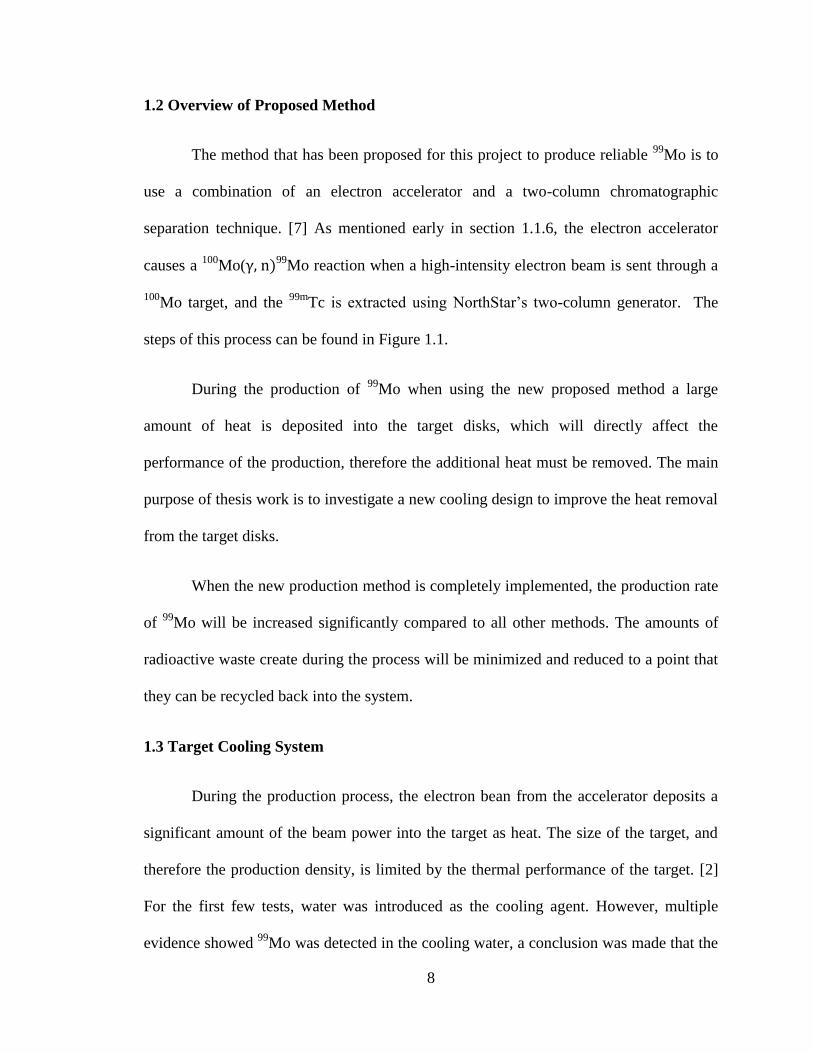
1.3.2 Once-through Cooling System
As a proof of principle, a once-through helium gas cooled target was
demonstrated using the electron accelerator facility at ANL in 2011. This cooling system
used 20 large compressed gas bottle of helium as the supply of the cooling gas. A picture
of the gas manifold and bottles is shown in Figure 1.2. [2]
The flow of the helium gas was regulated from the bottle manifold pressure down
to the target inlet pressure of ~2 MPa by a high flow regulator. Due to the expansion
through the regulator the helium gas became very cold; it was then passed through a gas
to water heat exchanger. To control the flow rate of the helium a regulating valve was
installed downstream of the target. From the regulating valve, the helium was passed
through a HEPA filter and exhausted into the room ventilation system. [2]

11
Figure 1.2: Photograph of the Helium Gas Bottle and Gas Manifold Used During the Once-through Helium
Gas Cooled Thermal Test Using the Electron Accelerator at ANL in March 2011
With the setup, a thermal test was conducted at ANL in 2011. The electron beam
used in the test was set as follows: 17 MeV, 10.3 KW, 6 mm FWHM. The twenty large
bottles of helium provided about 20 minutes of run time at full flow rate, and reached a
peak velocity of 200 m/s, which cooled of peak heat flux of ~800 . The result
from this experiment determined that the heat fluxes on the order of 1000 or
more were within reach with helium gas cooling. [2]
1.3.3 Closed Loop Helium Gas Cooling System
With the success of the once-through cooling system a closed loop helium gas
cooling system was designed and installed at ANL. The main driving force for the flow is
a three-lobe-roots-type blower, and it is contained within a pressurized system. A roots

12
blower is typically characterized by a high mass flow rate but a fairly low pressure rise
(~100 KPa). To achieve a high target inlet pressure of ~2 MPa (290 Psi), and hence a
higher gas density and mass flow rate, the roots blower is enclosed in a pressure vessel
that is pressurized very near the desired target inlet pressure. In this fashion, the roots
blower is only required to overcome the dynamic pressure losses in the system, which is
well within the capabilities of a roots blower, and not have to achieve the full static inlet
pressure of the target. A picture of the pressure vessel, roots blower, and motor installed
at ANL is shown in Figure 1.3. [2]
The schematic of the closed loop is shown in Figure 1.4 and an engineering
drawing of the layout in the accelerator vault is shown in Figure 1.5. From the blower
outlet on the pressure vessel, the helium gas is piped to a heat exchanger which serves as
an after cooler. The helium gas is heated as it is compressed by the blower, and the after
cooler is used to remove this heat. The helium is then piped to a filter to remove any oil
or particulates in the gas. From the filter, the helium is piped to the target. [2]
Temperature is monitored by a set of thermocouples installed on the inlet and
outlet of the target. Temperature data gathered from the thermocouples can be used to
calculate the power removed from the target.
In addition to the thermocouple, a simple screen filter is installed at the
downstream of the target to trap pieces of target if it were dissembled during the
irradiation. [2]
After helium left the filter, it passed through another heat exchanger which is used
to remove the heat absorbed in the helium from the target. From the heat exchanger, the

13
inlet temperature of the cooling water was~25 °C and the volumetric flow rate was ~11
gpm. After exiting from the second heat exchanger, the helium flowed through a coriolis
flow meter which is used to measure the mass flow rate of the helium. From the flow
meter, the helium is flowed back to the pressure vessel and the cycle starts all over again.
[2]
Similar loop is now built at LANL and ready to be used for the experimental part
of this project.
Figure 1.3: Photograph of the Roots Blower (Left) and Motor (Right) Mounted to a Plate Cantileverd of the
End of the Pressure Vessle Flange Plate. The Other End of the Pressure Vessel Slides Back and Forth Over
the Motor and Blower on Rails Bolted to the Skid Plate

14
Figure 1.4: P&ID of the Production System

15
Figure 1.5: Piping Layout for the Helium Target Cooling System.
1.3.4 Flow Properties
According to the energy equation shown in Eq.(1.1). [8] The heat transfer
coefficient is directly related to the mass flow rate. When the heat capacity and the
temperature difference are fixed; increase mass flow rate will directly increase the heat
transfer coefficient.
( (1.1)
Maximizing mass flow rate can be achieved by changing the target geometry and
the initial conditions of the flow loop. The main focus of this thesis project will be put on
the design of the target geometry. Assuming the initial condition of the flow loop has
already been maximized; a series of parametric studies on the target geometry will be

16
tested and compared. Close attention will be put on several parameters and they are:
maximum and average velocities at different section of the target, mass flow rate at the
inlet and outlet, and the dynamic pressure at the inlet region. The new design of the target
geometry should able to reduce the target wall temperature to between 550 °C and 650 °C
as described earlier in this chapter.
17
Chapter 2 - Theory and Methodology
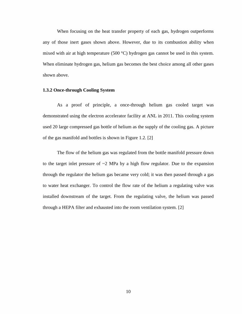
2.1 Mach Number Calculation
Mach number is simply described as ratio of object speed over speed of sound. It
is a dimensionless number that is useful for analyzing fluid dynamics problems to
determine if a flow can be treated as an incompressible flow. The Mach number can be
expressed as shown in Eq. (2.1). [9]
(2.1)
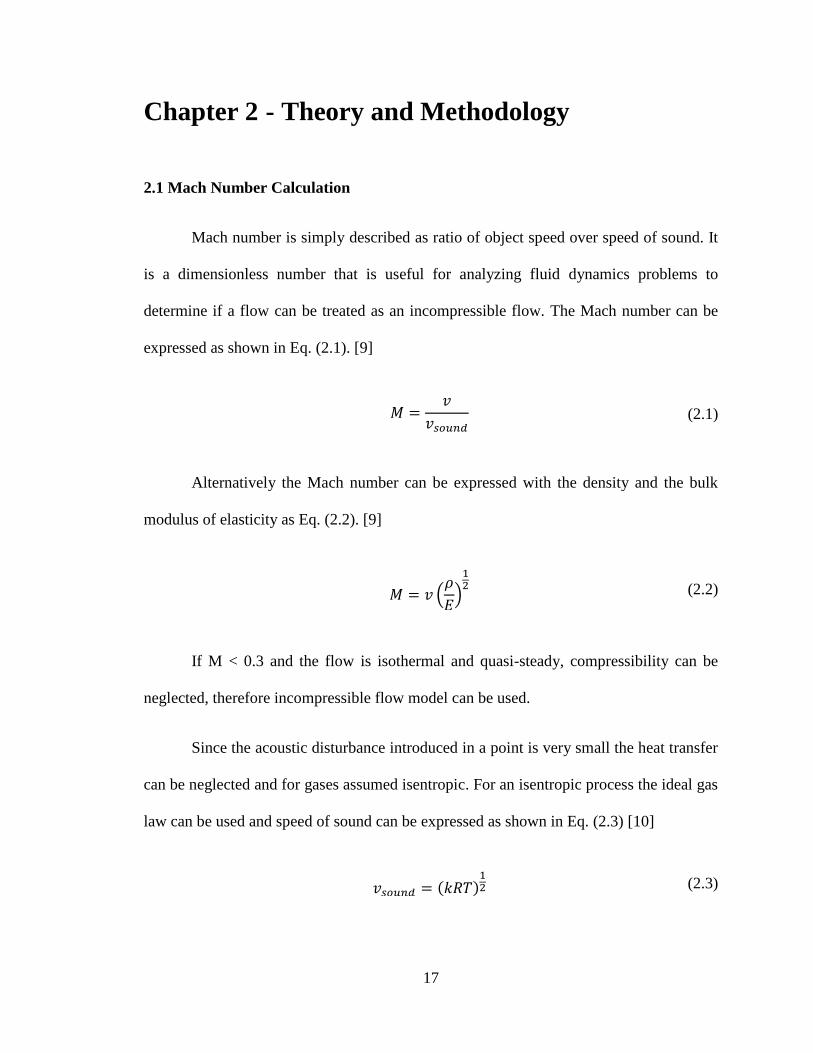
Alternatively the Mach number can be expressed with the density and the bulk
modulus of elasticity as Eq. (2.2). [9]
(
)
(2.2)
If M < 0.3 and the flow is isothermal and quasi-steady, compressibility can be
neglected, therefore incompressible flow model can be used.
Since the acoustic disturbance introduced in a point is very small the heat transfer
can be neglected and for gases assumed isentropic. For an isentropic process the ideal gas
law can be used and speed of sound can be expressed as shown in Eq. (2.3) [10]
( (2.3)

18
2.2 Density Calculation
Gases are highly compressible in comparison to liquids, which changes in density
directly related to changes in pressure and temperature through the Eq. (2.4) [11]
(2.4)
Eq. (2.4) is commonly termed the ideal or perfect gas law, or the equation of state
for an ideal gas. It is known to closely approximate the behavior of real gases under
normal conditions when the gases are not approaching liquefaction. [11]
2.3 Confined Flows
In many cases the fluid is physically constrained within a device so that its
pressure cannot be prescribed. Such cases include nozzles and pipes of variable diameter
for which the fluid velocity changes because the flow area is different from one section to
another. For these situations it is necessary to use the concept of conservation of mass
(the continuity equation) along with Bernoulli equation. Consider a fluid flowing through
a fixed volume that has one inlet and one outlet. If the flow is steady so that there is no
additional accumulation of fluid within the volume, the rate at which the fluid flows into
the volume must equal the rate at which it flows out of the volume (otherwise, mass
would not be conserved). [11]
The mass flow rate from an outlet can be calculated as shown in Eq. (2.5). [11]
(2.5)

19
The volume flow rate Q can be related directly to the cross-sectional area A, and
it can be expressed as shown in Eq. (2.6). [11]
(2.6)
Thus, mass flow rate can be reconstructed as shown in Eq. (2.7). [11]
(2.7)
To conserve mass, the inflow rate must equal the outflow rate. If the inlet is
designated as (1) and outlet as (2), it follows that . Thus, conservation of mass
requires [11]:
(2.8)
If the density remains constant, then , and the above becomes the
continuity equation for incompressible flow [11]:
(2.9)
2.4 Reynolds Number
The Reynolds number is undoubtedly the most famous dimensionless parameter
in fluid mechanics. It is named in honor of Osborne Reynolds (1842-1912), a British
engineer who first demonstrated that this combination of variables could be used as a
criterion to distinguish between laminar and turbulent flow. In most fluid flow problems
there will be a characteristic length, ℓ, and a velocity, V, as well as the fluid properties of
density, , and viscosity, , which are relevant variables in the problem. Thus, with these
variables the Reynolds number can be expressed as shown in Eq. (2.10). [11]

20
(2.10)
The Reynolds number is a measure of ratio of the inertia force on an element of
fluid to the viscous force on an element. When these two types of forces are important in
a given problem, the Reynolds number will play an important role. [11]
2.5 CFD Models
To properly characterize the flows that are in the cooling channels a turbulence
model is needed. The candidate turbulence model should be able to capture the fluid
interaction with the boundaries (walls) and initial conditions (inlet and outlet).
Initially both standard (SKW) and SST - (SSTKW) models were conducted for
this project; the final decision on the turbulence model will be validated and announced
in the later chapter. Many studies show that both SKW and SSTKW models agree
reasonably well with experimental data from Obi [12] and LES results from Kaltenback
[13]. In addition, both SKW and SSTKW models have been known to obtain good results
for flows that involve separation and reattachment.
Many commercial software packages are available for this CFD project and most
are constructed and configured in a similar fashion. They are usually integrated systems,
which include a mesh generator, a flow solver, and a visualization post processing tool.
Most of the CFD codes are using popular algorithms that are published in the literature,
for instance, standard - model from Wilcox [14] , SST - model developed by
Menter [15], and one of most popular models standard - model proposed by Launder

21
and Spalding [16]. The selections of these models are based on their robustness and
reliability.
There are many popular commercial software packages recommended by multiple
literatures, and they are CFX, Fluent, and Star-CD. However, ANSYS Fluent 14.5
version is chosen by the recommendation from El-Behery’s [17] asymmetric diffuser
study. The models comparison and their theory behind them are presented in section
2.5.1.
2.5.1 Turbulence Models
The commercial code ANSYS Fluent solves a set of governing equations. The
numerical method employed is based on the finite volume approach. Fluent provides
flexibility in choosing discretization schemes for each governing equation. The
discretized equations, along with the initial condition and boundary conditions, are solved
using the segregated solution method. Using the segregated solver, the conservation of
mass and momentum are solved sequentially and a pressure correction equation is used to
ensure the conservation of momentum and the conservation of mass (continuity
equation). Several turbulence models, such as, the standard k-ε model, the low-Re k-ε
model, the standard k- model, the shear-stress transport k- model, the Reynolds stress
model (RSM) and the - model are used in the literature to predict the separating flow
through diffuser. [17] The first five models are available directly in FLUENT while the
last one ( - model) was implemented using user-defined functions (UDF) and user-
defined scalars (UDS).
The steady Reynolds Averaged Navier-Stokes (RANS) equations for turbulent

22
incompressible fluid flow with constant properties are used in the present study. The
governing flow field equations are the continuity and the RANS equations, which are
given by [18]:
(2.11)
Where is the main strain rate and calculated by [18]:
It is an unfortunate fact that no single turbulence model is universally accepted as
being superior for all classes of problems. The choice of turbulence model will depend on
considerations such as the physics of the flow, the established practice for a specific class
of problem, the level of accuracy required, the available computational resources, and the
amount of time available for the simulation. To make the most appropriate choice of
model for ones’ application, one needs to understand the capabilities and limitations of
the various options. [18]
However, in the literature, many results show that standard - , SST - , and
- models clearly performed better than other models. They show an acceptable
agreement with the velocity and turbulent kinetic energy profiles provided by Obi [12],
Buice, and Eaton [19]. Since - model cannot be directly obtained from ANSYS Fluent
(
(2.12)
(
)
(2.13)

23
and requires additional UDF and UDS, standard and SST - models are more suitable
than - model. Standard and SST - models can be directly obtained from ANSYS
Fluent, and the ANSYS FLUENT Theory Guide gives a detailed explanation on standard
and SST - model as well as other popular turbulent models.
For this project, only three turbulent models are reviewed and all three of them
are used to compare against the experimental data provided by Buice and Eaton. The
three models are: Standard - , Standard - , and SST - models. By doing the
comparison, one can prove that the new FLUENT solver can still be valid to obtain a
reliable solution as El-Behery did with FLUENT 6.3.26 version.
Two-equation models are historically the most widely used turbulence models in
industrial CFD. They solve two transport equations and model the Reynolds Stresses
using the Eddy Viscosity approach. The standard k-ε model in ANSYS FLUENT falls
within this class of models and has become the workhorse of practical engineering flow
calculations in the time since it was proposed by Launder and Spalding [16]. Robustness,
economy, and reasonable accuracy for a wide range of turbulent flows explain its
popularity in industrial flow and heat transfer simulations. The drawback of some k-ε
models is their insensitivity to adverse pressure gradients and boundary layer separation.
They typically predict a delayed and reduced separation relative to observations. This can
result in overly optimistic design evaluations for flows, which separate, from smooth
surfaces (aerodynamic bodies, diffusers, etc.). The k-ε model is therefore not widely used
in external aerodynamics [18].
The standard k-ε model is a model based on model transport equations for the

24
turbulence kinetic energy ( ) and its dissipation rate ( ). The model transport equation
for k is derived from the exact equation, while the model transport equation for was
obtained using physical reasoning and bears little resemblance to its mathematically exact
counterpart [18].
The standard k-ε model is valid only for fully turbulent flow. It assumes that the
flow is fully turbulent, and the effects of molecular viscosity are negligible [18].
The turbulence kinetic energy, k, and its rate of dissipation, are obtained from
the following transport equations:
In these equations, represents the generation of turbulence kinetic energy due
to the mean velocity gradients. is the generation of turbulence kinetic energy due to
buoyancy. represents the contribution of the fluctuating dilation in compressible
turbulence to the overall dissipation rate. and are constants. and are
turbulent Prantl numbers for and , respectively. and are user-defined source
terms [18].
The standard - model in ANSYS FLUENT is based on the Wilcox model [14] ,
which incorporates modifications for low-Reynolds number effects, compressibility, and
t( k
xi( kui
xj*(
t
k) k
xj + Gk Gb ε Sk
And
(2.14)
(
(
[(
)
]
( -
(2.15)
25
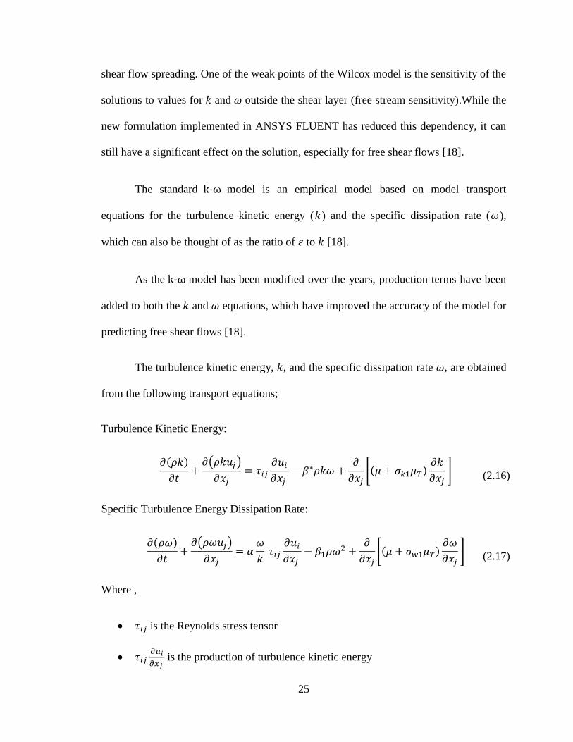
shear flow spreading. One of the weak points of the Wilcox model is the sensitivity of the
solutions to values for and outside the shear layer (free stream sensitivity).While the
new formulation implemented in ANSYS FLUENT has reduced this dependency, it can
still have a significant effect on the solution, especially for free shear flows [18].
The standard - model is an empirical model based on model transport
equations for the turbulence kinetic energy ( ) and the specific dissipation rate ( ),
which can also be thought of as the ratio of to [18].
As the - model has been modified over the years, production terms have been
added to both the and equations, which have improved the accuracy of the model for
predicting free shear flows [18].
The turbulence kinetic energy, , and the specific dissipation rate , are obtained
from the following transport equations;
Turbulence Kinetic Energy:
Specific Turbulence Energy Dissipation Rate:
Where ,
is the Reynolds stress tensor
is the production of turbulence kinetic energy
(
( )
*(
+ (2.16)
(
( )
*(
+ (2.17)
26
is the dissipation of turbulence kinetic energy
is the production of specific turbulence energy dissipation rate
is the dissipation of the specific turbulence energy dissipation rate
are closure coefficients
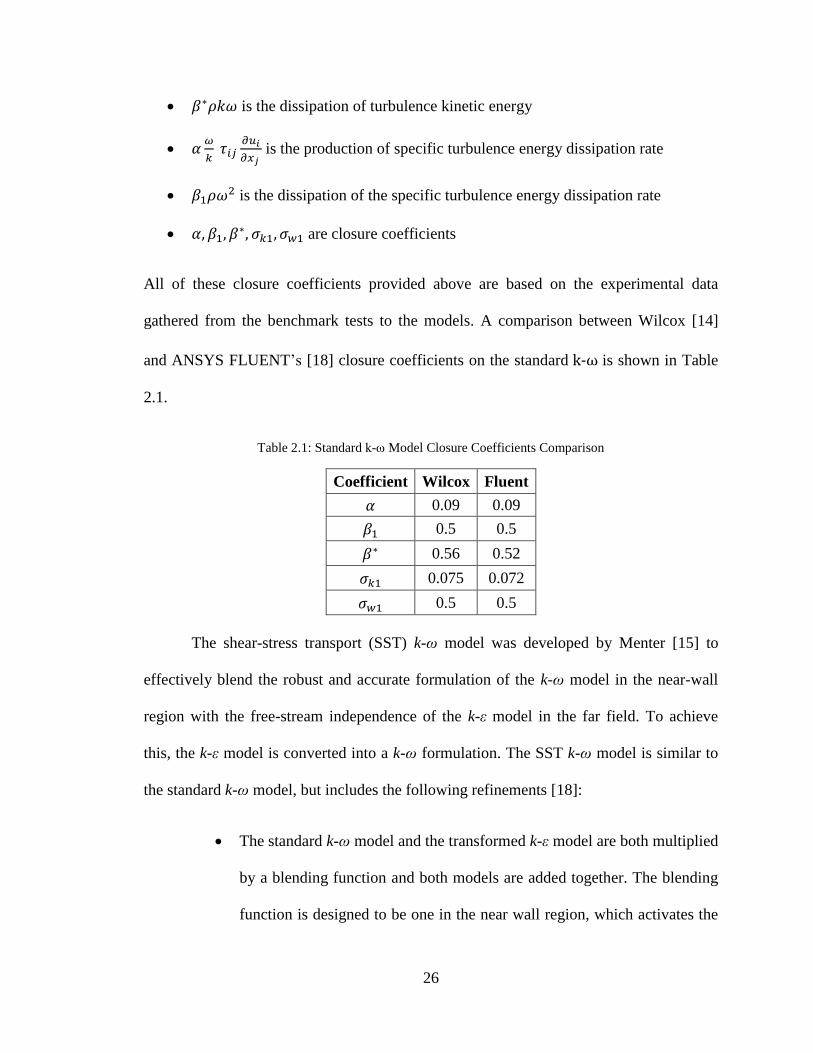
All of these closure coefficients provided above are based on the experimental data
gathered from the benchmark tests to the models. A comparison between Wilcox [14]
and ANSYS FLUENT’s [18] closure coefficients on the standard - is shown in Table
2.1.
Table 2.1: Standard k- Model Closure Coefficients Comparison
Coefficient Wilcox Fluent
0.09 0.09
0.5 0.5
0.56 0.52
0.075 0.072
0.5 0.5
The shear-stress transport (SST) k-ω model was developed by Menter [15] to
effectively blend the robust and accurate formulation of the k-ω model in the near-wall
region with the free-stream independence of the k-ε model in the far field. To achieve
this, the k-ε model is converted into a k-ω formulation. The SST k-ω model is similar to
the standard k-ω model, but includes the following refinements [18]:
The standard k-ω model and the transformed k-ε model are both multiplied
by a blending function and both models are added together. The blending
function is designed to be one in the near wall region, which activates the

27
standard k-ω model, and zero away from the surface, which activates the
transformed k-ε model.
The SST model incorporates a damped cross diffusion derivative term in
the ω equation.
The definition of the turbulent viscosity is modified to account for the
transport of the turbulent shear stress.
The modeling constants are different.
These features make the SST k-ω model more accurate and reliable for a wider
class of flow (for example, adverse pressure gradient flows, airfoils, transonic shock
waves) than the standard k-ω model.
Menter’s SST k-ω model is formulated in the form of:
Turbulence Kinetic Energy:
Specific Turbulence Energy Dissipation Rate:
Where the blending function ( , and can be obtained as follow:
(
( )
*(
+ (2.18)
(
( )
–
[(
]
(
(2.19)

28
Where variable y is the distance from the nearest wall. Table 2.2 shows the closure
coefficient between Menter [15] and fluent [18] model.
Table 2.2: SST - Model Closure Coefficients Comparison
Coefficient Menter Fluent
0.85 1.176
1.0 1.0
0.5 2.0
0.856 1.168
0.31 0.31
0.075 0.075
0.09 0.0828
A benchmark problem constructed by El-Behery [17] will be used in Chapter 3 to
validate the candidate turbulence models mentioned in this section.
* (√
)
+ (2.20)
(
)
(2.21)

29
Chapter 3 - CFD Model Development
This section describes the CFD model development by using the ANSYS Fluent
14.5 software package. Two separate cases were studied for the 99
Mo project; one for
simple single channel flow and other for complex multi-channels flow.
For single channel study, both El-Behery [17] and Lan’s [20] experimental
comparison data were used to validate the model chosen for this project. For multi-
channel case, the CFD result was compared directly to in-house experimental data that
was measured at LANL.
From the initial comparison, single channel is more for an academic study, which
represents the ideal case of a simple flow through a channel. The single channel study has
been well published in the literature. A benchmark problem from El-Behery’s study was
used to finalize the turbulence model use for this project. A parametric study on the
diffuser angle was conducted and a correlation between diffuser angle and flow
separation was developed and compared against Lan’s result. In this study, an ideal case
can be obtained; with certain diffuser angles the flow separation can be completely
eliminated. Even though, the single channel study does not directly reflect the actual
behavior of the fluid flow that is performed from the actual production, it is still useful
when trying to get a quick solution when optimizing the channel geometry, it can be used
to eliminate some of the design process for the multi-channels model. When it comes to
computational performance, single channel requires much less computational time than
the multi-channel study and still produces a reasonable result.

30
For multi-channels study, since the ideal flow can never been obtained, a
complete different flow behavior was found compared to the single channel study.
However, this study is more valuable than the single channel study for the 99
Mo project,
since the actual production involves multiple targets and cooling channels. Since the flow
separation can no longer be eliminated, reducing the flow separation has become the
priority for this part of study. The result of this study is later compared to the experiment
that is conducted in-house.
3.1 Geometry
For ANSYS Fluent, the very first step of the simulation is to construct geometry.
An exploded ISO view of the target disks and holder is shown in Figure 3.1.
Figure 3.1: Exploded ISO view of housing, holder, and targets. Tubes that are located at the holder chimney
flange are for thermocouple insertion.

31
To aid in mounting and aligning the target to the accelerator beam pipe, the target
assembly was mounted inside a vacuum cube, as shown in Figure 3.2.
Figure 3.2: Cross-section view of Mo99 Target and Vacuum Cube Assembly showing assembly and weld
locations.
For CFD simulation not all components are required to be modeled, the focus of
this project is to model the test section, which only includes the 100
Mo target disks and
the cooling channels in between the target disks.
The original configuration for the target disk was 12 mm in diameter and 1 mm
thick, and featuring 0.5 mm wide channels in between disks. However, to increase the
production rate a new configuration of the disk and the cooling channel is implemented.
The target disk diameter is still 12 mm but with half of the thickness (0.5 mm), and there
is also a 50% reduction (0.25 mm) on the width of the cooling channel. With the newest
configuration of the target disk and the new design of the target holder, the total number
of disks that can be fitted in the test section is now 82 instead of 25.

32
Figure 3.3 gives a demonstration of the configuration of the test section (this
figure might not reflect to the actual production configuration). Two electron beams
instead of one will be shot through the windows on both sides (front and back) normal to
the disk faces, which will result in increase in production rate.
Figure 3.3: Target Disks and Production Configuration
3.2 Single Channel Model
The early phase of this project was to model a single helium flow channel instead
of all cooling channels (83 channels). The main reason of doing this step is to quickly
develop some fundamental knowledge of the fluid flow, and as mentioned before the
result from the single channel study will also be used to eliminate some of the design
process for the multi-channels model.
A base case CFD model was constructed to represent the original target cooling
channel. The original target cooling channel has a sudden contraction and expansion inlet
and outlet. Losses occur because of sudden change of inlet and outlet area. Because the
fluid cannot turn a sharp right-angle corner, the flow is separated from the sharp corner,

33
which creates recirculation. The majority of the inlet head loss is due to inertia effects
that are eventually dissipated by the shear stresses within the fluid. Only a small portion
of the loss is due to the wall shear stress within the inlet region. The net effect is that the
loss coefficient for a sudden contraction inlet could be high as , which means
that one-half of a velocity head is lost as the fluid enters the channel. A similar effect
applies to the outlet region, as the fluid leaves the smaller area and initially forms a jet-
type structure as it enters the larger area. Within a few diameters downstream of the
expansion, the jet becomes dispersed across the channel, and fully developed flow
becomes established again. During this process, a portion of the kinetic energy of the
fluid is dissipated as a result of viscous effects. [11] A demonstration of the original
target cooling channel can be found in Figure 3.4.
Figure 3.4: Original Target Cooling Channel (Single Channel Base Case)
An obvious way to reduce the loss is to add a more efficient feature to replace the
sudden contraction and expansion inlet and outlet. Two designs were proposed for the
inlet section; rounded and angled entrance. A diffuser design was introduced to minimize
the loss coefficient at the outlet section. A comparison and final decision of the inlet and
outlet features will be shown in Chapter 4 where the final result is provided.
[m/s]

34
3.2.1 Turbulence Model Validation
The fundamental process of turbulent flow separation has long been a
troublesome calculation in the development of numerical turbulence models. Part of this
difficulty can be traced to a limited database of experimental results for validation of flow
models. Studies of turbulent flow in an asymmetric plane diffuser have been conducted
independently by Obi et al [12]. and Buice and Eaton [19]. Using the experimental data
of Buice as a benchmark, many studies had been conducted both experimentally and
numerically on plane asymmetric diffusers. Many studies are compared to the results
from turbulence models of varying complexity and their ability to accurately resolve the
locations of separation and reattachment, as well as the velocity profiles through the
diffuser. [21]
Figure 3.5: Obi's Diffuser Geometry
Figure 3.5 [12] shows the geometry of one of the very first asymmetric turbulent
diffuser studies conducted by Obi et al [12]. The goal of his study was to validate a
second-moment closure turbulence model for non-orthogonal numerical grids. A single-

35
component Laser Doppler Velocimetry (LDV) system was implemented with a Bragg cell
frequency shift in a forward-scatter configuration. [21]
To validate the models that are used in this project, a benchmark problem was
conducted. Figure 3.6, shows the popular benchmark problem that was constructed by El-
Behery. He modeled the similar domain as Buice and Eaton did in their experiment and
ran series of turbulent models on it. The axial velocity profile through the diffuser for the
tested turbulent models was calculated and used to compare the experimental data
gathered by Buice and Eaton.
Figure 3.6: Development of axial velocity profile through the diffuser for the tested turbulence models
compared with an experimental result of Buice-Eaton data. [19]
The result shown in Figure 3.6 is clear that the best model for diffuser flow are
- , Standard - , and SST - model. These three models were able to predict the
right physics from the experiment.

36
Figure 3.7: Mean Stream Velocity Comparison in a 10-Degree Diffuser (Model Validation)
By re-running El-Behery’s simulation in ANSYS Fluent 14.5, three models were
used to compare to Buice and Eaton’s experimental data. In Figure 3.7, both standard and
SST - models show a better sign when matching the experimental data than standard
- model. This validation process proves that both standard and SST - models are
good candidates for this research project. However, a further testing and comparison are
needed to confirm which model is truly the best model for the 99
Mo project.
3.2.2 Boundary Conditions and Model Inputs
The three-dimensional cooling channel model has three main parts: upstream inlet
section, center cooling channel, and downstream outlet section with a diffuser design. All
dimensions used in the simulation are reflected to the most current design that is sitting in
the laboratory. The upstream inlet section has a duct height of 10.16 mm and width of
37
0.75 mm and featuring either a rounded or angled inlet (To be determined in next
chapter). The center channel is constructed as a simple duct with duct height of 10.16 mm
and width of 0.25 mm resulting in an expansion ratio of 3. Finally the downstream outlet
section is featuring a diffuser design connected with an identical duct as the inlet section.
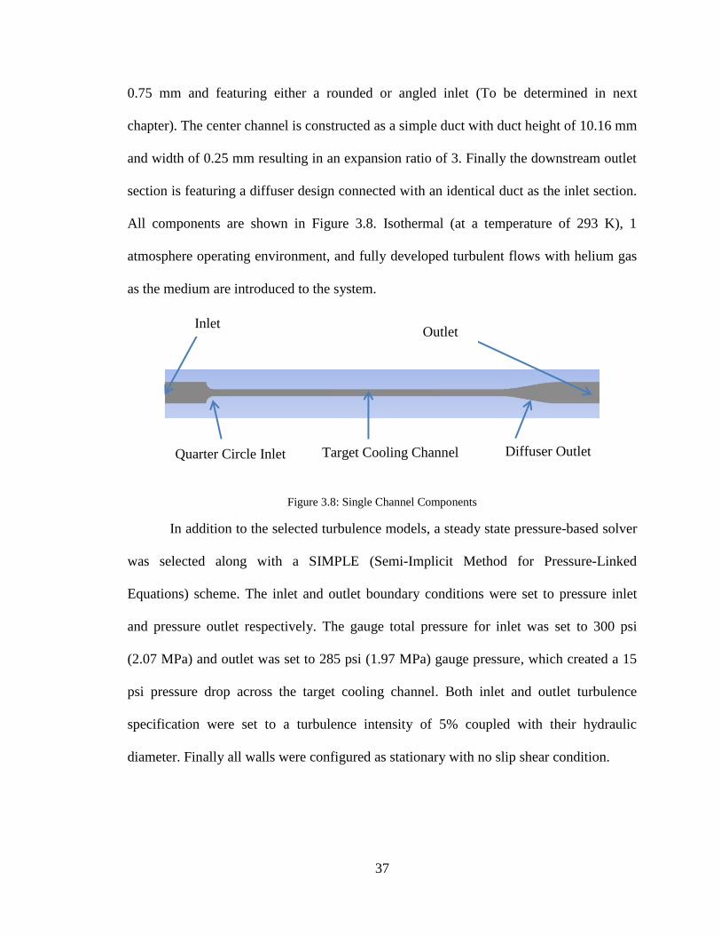
All components are shown in Figure 3.8. Isothermal (at a temperature of 293 K), 1
atmosphere operating environment, and fully developed turbulent flows with helium gas
as the medium are introduced to the system.
Figure 3.8: Single Channel Components
In addition to the selected turbulence models, a steady state pressure-based solver
was selected along with a SIMPLE (SemiImplicit Method for PressureLinked
Equations) scheme. The inlet and outlet boundary conditions were set to pressure inlet
and pressure outlet respectively. The gauge total pressure for inlet was set to 300 psi
(2.07 MPa) and outlet was set to 285 psi (1.97 MPa) gauge pressure, which created a 15
psi pressure drop across the target cooling channel. Both inlet and outlet turbulence
specification were set to a turbulence intensity of 5% coupled with their hydraulic
diameter. Finally all walls were configured as stationary with no slip shear condition.
Target Cooling Channel Diffuser Outlet Quarter Circle Inlet
Inlet Outlet

38
3.2.3 Mesh Development
A series of mesh resolution studies were conducted for all cases. A sample of
rounded quarter circle inlet and 10-degree diffuser outlet is used in this section to show
the grid independency of the simulation (See Figure 3.9 and Figure 3.10). A mesh biasing
technique was introduced into this project, which is a non-uniform structured
computational grid, where the finer grid is placed near the solid wall and region where
the boundary layer is affective. With the higher grid density near the wall it is sufficient
to capture the action near the boundary layer. In this study, growth ratio for the mesh was
set to be no more than 1.2, which will help to keep the aspect ratio in a reasonable range.
Figure 3.9: A Typical Mesh Used in the Calculation - Quarter Circle Inlet (438,216 Nodes)
Figure 3.10: A Typical Mesh Used in the Calculation - Diffuser Outlet (438,216 Nodes)
Boundary layer theory was used to calculate the distance from the first boundary
layer to the wall. The calculation for the distance to the wall is provided below:
(3.1)

39
Where,
= Reynolds number
= Kinematic viscosity
= Skin friction
= Wall shear stress
= Friction velocity
= Distance to the nearest wall
= Non-dimensional wall distance
Since the standard and SST - models were chosen for this project, the
recommendation from ANSYS fluent [18] is to use . With input of Reynolds
number the distance to the nearest wall y was calculated to be
m. As a result, higher grid density was placed near wall than the center of
the channel. An evidence of the mesh biasing result can also be found in Figure 3.9 and
(3.2)
[ ( ] (3.3)
(3.4)
√
(3.5)
(3.6)
40
Figure 3.10.
Mesh matrix was constructed to determine the independence of the model. To
ensure the quality of each mesh configuration, two mesh quality measurements were used
to determine the quality of the mesh; orthogonal quality and skewness. More information
on these two measurements can be found as follows:
Orthogonal Quality:
Orthogonal Quality ranges from 0 to 1, where values close to 0 correspond
to low quality and value close to 1 correspond to high quality.
Skewness:
Minimize equiangle skew:
1. Hex and quad cells: skewness should not exceed 0.85.
2. Tri’s: skewness should not exceed 0.85.
3. Tets: skewness should not exceed 0.9.
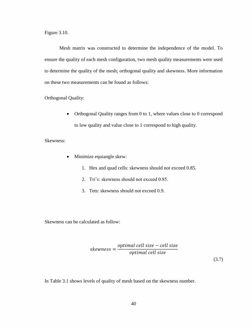
Skewness can be calculated as follow:
In Table 3.1 shows levels of quality of mesh based on the skewness number.
(3.7)

41
Table 3.1: Mesh Skewness
Value of
Skewness
0-0.25 0.25-0.50 0.50-0.80 0.80-0.95 0.95-0.99 0.99-1.00
Cell Quality excellent good acceptable poor sliver degenerate
Three sets of meshes were compared as shown in Table 3.2.
Table 3.2: Single Channel Mesh Metrics
Turbulence
Model
# of
Nodes
# of
Elements
Orthogonal
Quality
Skewness Mass
Flow
(g/s)
Max
Channel
Velocity
(m/s)
Max Inlet
Velocity
(m/s)
SKW 59,136 51,750 0.986 2.29E-02 1.70 230.1 66.6
SKW 438,216 409,500 0.992 1.31E-02 1.76 259.0 69.1
SKW 788,020 742,800 0.994 1.14E-02 1.78 260.0 69.9
SSTKW 59,136 51,750 0.986 2.29E-02 1.90 259.6 74.2
SSTKW 438,216 409,500 0.992 1.31E-02 1.94 269.3 75.8
SSTKW 788,020 742,800 0.994 1.14E-02 1.94 270.3 75.9
All meshes provided in Table 3.2 were constructed as hex element; according to
the two mesh quality measurements used in this study, all meshes studied here were high
quality meshes. The mass flow, max channel velocity, and max inlet velocity data show a
good sign of mesh convergence and independence when number of nodes reaches around
438,216. The mesh independence can also be proven visually by plotting the velocity
profile along the mid-section of the channel. If the meshes are converged and have
reached independence; their velocity profiles should be similar or close to each other. The
visual evidence of mesh independence can be found in Figure 3.11 and Figure 3.12.
As expected from the result shown in Table 3.2; both Figure 3.11 and Figure 3.12
show good signs of mesh convergence. For both cases, the mid-section velocity profile
for 438,216 nodes is almost completely overlaid on the velocity profile for 788,020
nodes. It is a sign of convergence and independence when two different high quality
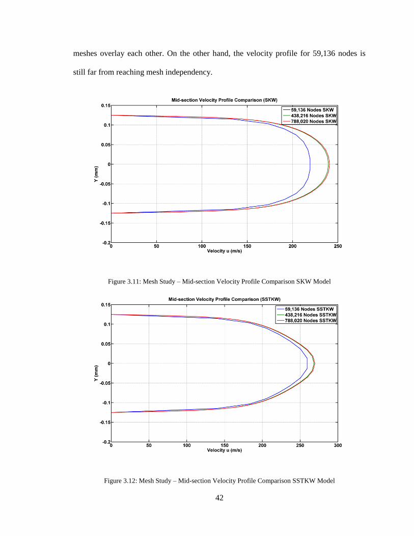
42
meshes overlay each other. On the other hand, the velocity profile for 59,136 nodes is
still far from reaching mesh independency.
Figure 3.11: Mesh Study – Mid-section Velocity Profile Comparison SKW Model
Figure 3.12: Mesh Study – Mid-section Velocity Profile Comparison SSTKW Model

43
An example of different mesh configurations can be found as follows:
Figure 3.13: Mesh Configuration - 59,136 Nodes Inlet
Figure 3.14: Mesh Configuration - 438,216 Nodes Inlet
Figure 3.15: Mesh Configuration - 788,020 Nodes Inlet
[m/s]
[m/s]
[m/s]

44
Figure 3.16: Mesh Configuration – 59,136 Nodes Outlet
Figure 3.17: Mesh Configuration - 438,216 Nodes Outlet
Figure 3.18: Mesh Configuration - 788,020 Nodes Outlet
[m/s]
[m/s]
[m/s]

45
Figure 3.19: Mesh Configuration - 59,136 Nodes ISO View
Figure 3.20: Mesh Configuration - 438,216 Nodes ISO View
[m/s]
[m/s]

46
Figure 3.21: Mesh Configuration - 788,020 Nodes ISO View
3.2.4 Result Monitoring
To determine whether the result is converged and reached steady state or not
many criteria were monitored. The most common criteria to be monitored are the default
scaled residuals from ANSYS Fluent. There are six residuals being monitored for the
standard and SST - model and they are: Continuity, x-velocity, y-velocity, z-velocity,
turbulence kinetic energy (k), and specific dissipation rate ( ). All residuals errors were
set to 1e-6 to ensure steady state and convergence. A sample of scaled residuals can be
found in Figure 3.22.
In addition to the scaled residuals, many other criteria can be monitored. Two
additional criteria were monitored during the simulation: dynamic pressure at the inlet
and mass flow rate at the outlet. Once the simulation is reached steady state these two
criteria should become stable, in another word, they should stay (almost) constant. These
[m/s]

47
two criteria become extremely helpful when determining mesh convergence and
independence for multi-channels simulation. Figure 3.23 and Figure 3.24 shown the
solution is converged and reached steady state.
Figure 3.22: Scaled Residuals - Single Channel

48
Figure 3.23: Mass Flow Rate @ Outlet - Single Channel
Figure 3.24: Dynamic Pressure @ Inlet - Single Channel

49
3.3 Multi-Channels Model
Similar procedures were used for the multi-channel model; since the initial and
boundary conditions are the same as the single channel model.
3.3.1 Multi-Channels Boundary Conditions and Model Inputs
Multi-channel model was constructed by stacking numbers of single channel in
parallel. Similar to the single channel model, multi-channels model also has three main
parts: upstream inlet section, center cooling channel, and downstream outlet section with
a diffuser design. The upstream inlet section has a duct height of 10.16 mm; the width of
the inlet section will depended on the number of channels that are required to be
simulated. The inlet section was constructed long enough to allow the fluid to become
fully developed before it enters the center channel. A rounded or angled inlet will be
determined in next chapter. No change on the center channel, for each channel, it was
constructed as a simple duct with duct height of 10.16 mm and width of 0.25 mm. Finally
the downstream outlet section is featuring a diffuser design connected with an identical
duct as the inlet section. All components are shown in Figure 3.25. Isothermal (at a
temperature of 293 K), 1 atmosphere operating environment, and fully developed
turbulent flows with helium gas as the medium are introduced to the system.

50
Figure 3.25: Multi-Channels Components
Same as the single channel simulation, a steady state pressure-based solver was
selected along with a SIMPLE (SemiImplicit Method for PressureLinked Equations)
scheme. The inlet and outlet boundary consitions were set to pressure inlet and pressure
outlet respectively. The gauge total pressure for inlet was set to 300 psi (2.07 MPa) and
outlet was set to 285 psi (1.97 MPa) gauge pressure, which created a 15 psi pressure
across the target cooling channel. Both inlet and outlet turbulence specification were set
to a turbulence intensity of 5% coupled with their hydraulic diameter. Finally all walls
were configured as stationary with no slip shear condition. To save computational time,
symmetry boundary condition was used for the multi-channel simulation. As shown in
Figure 3.25, symmetry boundary conditions were used on both side of the wall, This
Inlet
Quarter Circle Inlet
Target Cooling
Channel
Outlet
Diffuser Outlet
Symmetry Plane
Symmetry Plane

51
allows us to only construct 1/10 of the entire domain and still maintain an accurate result.
More detail on the 1/10 model will be explained in the later section.
3.3.2 Multi-Channels Mesh Development
Mesh development becomes extremely difficult when it comes to multi-channels
simulation. The difficulty comes from the complexity of the transition region. Multiple
mesh refinements are needed to develop a convergence and independence mesh.
Mesh biasing technique was also used for the multi-channels model; a growth
ratio of 1.2 is enforced to keep the aspect ratio in a reasonable range. A sample of
rounded quarter circle inlet and 4-degree diffuser outlet is used here to show the grid
independency of the simulation (See Figure 3.26, Figure 3.27, and, Figure 3.28).
Figure 3.26: Quarter Circle Inlet (2,392,054 Nodes Velocity Contour) - Multi-Channels
[m/s]

52
Figure 3.27: Diffuser Outlet (2,392,054 Nodes Velocity Contour) - Multi-Channels
Figure 3.28: Diffuser Outlet (2,392,054 Nodes Velocity Contour) - Close Up
[m/s]
[m/s]

53
Three different meshes are evaluated in this study. Orthogonal quality and
skewness are also used to monitor the quality of each mesh. Dynamic pressure at the
inlet, mass flow rate at the outlet, and maximum inlet velocity are compared between
different meshes. Mesh convergence and independence can be determined from the
comparison. Table 3.3 shows the comparison below:
Table 3.3: Multi-Channels Mesh Matrix (3 Degree Diffuser)
Turbulence
Model
# of
Nodes
# of
Elements
Orthogonal
Quality
Skewness Dynamic
Pressure
(Psi)
Max Inlet
Velocity
(m/s)
Mass
Flow
Rate (g/s)
SKW 1,594,242 1,400,256 0.978 6.42E-02 0.81 57.47 4.01
SKW 2,392,054 2,139,007 0.972 7.89E-02 0.79 56.97 3.97
SKW 3,276,750 2,945,782 0.977 6.43E-02 0.79 56.99 3.98
SSTKW 1,594,242 1,400,256 0.978 6.42E-02 1.86 73.52 4.95
SSTKW 2,392,054 2,139,007 0.972 7.89E-02 1.85 72.00 5.02
SSTKW 3,276,750 2,945,782 0.977 6.43E-02 1.85 71.62 5.02
In Table 3.3, three criteria monitored during the calculation shows little to no
difference. To ensure mesh convergence and independence are reached, the entire range
of scaled residuals and dynamic pressure data were monitored during the calculation. A
demonstration is shown below by using the SSTKW model:

54
Figure 3.29: Scaled Residuals – Multi-Channels (1,594,242 nodes) SSTKW
Figure 3.30: Scaled Residuals – Multi-Channels (2,392,054 nodes) SSTKW

55
Figure 3.31: Scaled Residuals - Multi-Channels (3,276,750 nodes) SSTKW
All residuals for 1,594,242 nodes mesh (Figure 3.29) are higher than rest of the
mesh setups. High oscillations are also shown on all residuals in Figure 3.29.
Figure 3.32: Inlet Dynamic Pressure - Multi-Channels (1,594,242 nodes) SSTKW

56
Figure 3.33: Inlet Dynamic Pressure - Multi-Channels (2,392,054 nodes) SSTKW
Figure 3.34: Inlet Dynamic Pressure - Multi-Channels (3,276,750 nodes) SSTKW
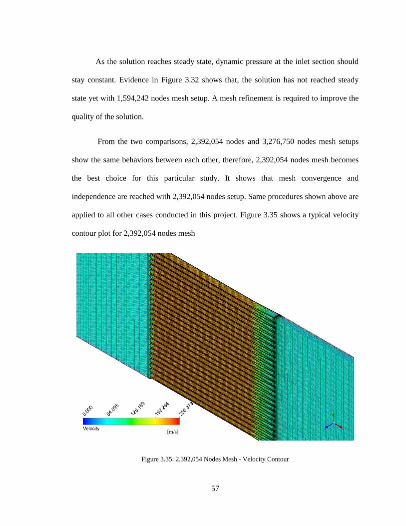
57
As the solution reaches steady state, dynamic pressure at the inlet section should
stay constant. Evidence in Figure 3.32 shows that, the solution has not reached steady
state yet with 1,594,242 nodes mesh setup. A mesh refinement is required to improve the
quality of the solution.
From the two comparisons, 2,392,054 nodes and 3,276,750 nodes mesh setups
show the same behaviors between each other, therefore, 2,392,054 nodes mesh becomes
the best choice for this particular study. It shows that mesh convergence and
independence are reached with 2,392,054 nodes setup. Same procedures shown above are
applied to all other cases conducted in this project. Figure 3.35 shows a typical velocity
contour plot for 2,392,054 nodes mesh
Figure 3.35: 2,392,054 Nodes Mesh - Velocity Contour
[m/s]

58
Chapter 4 – Design Decision and Model Reduction
In this chapter a series of CFD results for both single channel model and multi-
channels model are documented. As mentioned in previous chapter, inlet feature will be
determined in this chapter. Two potential candidates were proposed for this project:
quarter circle and 45° angled inlet. A side by side comparison along with base case
design (sudden contraction and expansion) will be shown in this chapter. A final decision
will be made in this chapter for the inlet feature.
The number one goal for this project is to maximize the flow rate to reduce extra
heat created by the system process. In addition to the inlet feature, a diffuser outlet is
added to the system to help guide the flow out of cooling section. A series of diffuser
angles are tested in later section of this chapter. A design will be finalized at the end of
this chapter. To validate the CFD models developed for this project; results gathered from
this chapter will be compared against a series of in-house experimental data. The
comparisons with the data will be shown in the next chapter.
4.1 Inlet Feature Selection
As mentioned earlier, two features were proposed for the inlet section: quarter
circle and 45° angled inlet. A visual representative for both features can be found in
Figure 4.1 and Figure 4.2. Both geometries feature a sudden expansion outlet, this outlet
can be found in Figure 4.3.

59
Figure 4.1: Quarter Circle Inlet
Figure 4.2: 45° Angled Inlet
Figure 4.3: Sudden Expansion Outlet
Both geometries are supplied with 300 Psi pressure at the inlet and configured to
have 15 Psi pressure drop across the channel. A pressure based and time steady solver is
used for both geometries. The results from both cases will be directly compared to the
base case shown in Figure 3.4
Figure 4.4 and Figure 4.5 show the results for the steady state solution for both
quarter circle inlet and 45° angled inlet, respectively. From the visual comparison, quarter
circle inlet has a better performance in velocity than the 45° angled inlet. However, only
looking at the maximum velocity does not tell the whole story, more details need to be
investigated to make the final conclusion.
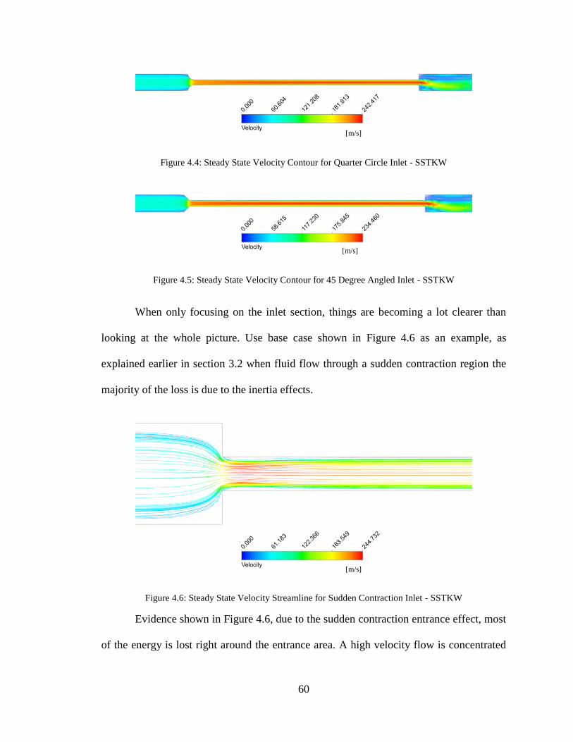
60
Figure 4.4: Steady State Velocity Contour for Quarter Circle Inlet - SSTKW
Figure 4.5: Steady State Velocity Contour for 45 Degree Angled Inlet - SSTKW
When only focusing on the inlet section, things are becoming a lot clearer than
looking at the whole picture. Use base case shown in Figure 4.6 as an example, as
explained earlier in section 3.2 when fluid flow through a sudden contraction region the
majority of the loss is due to the inertia effects.
Figure 4.6: Steady State Velocity Streamline for Sudden Contraction Inlet - SSTKW
Evidence shown in Figure 4.6, due to the sudden contraction entrance effect, most
of the energy is lost right around the entrance area. A high velocity flow is concentrated
[m/s]
[m/s]
[m/s]
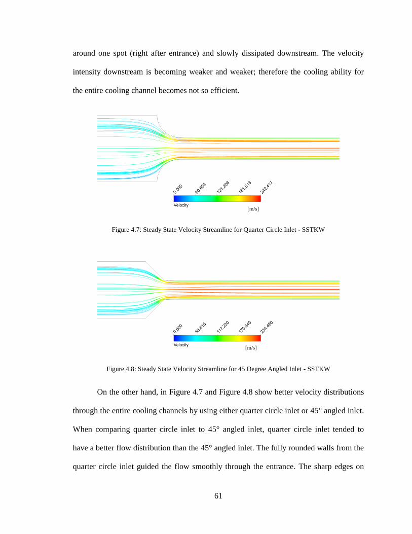
61
around one spot (right after entrance) and slowly dissipated downstream. The velocity
intensity downstream is becoming weaker and weaker; therefore the cooling ability for
the entire cooling channel becomes not so efficient.
Figure 4.7: Steady State Velocity Streamline for Quarter Circle Inlet - SSTKW
Figure 4.8: Steady State Velocity Streamline for 45 Degree Angled Inlet - SSTKW
On the other hand, in Figure 4.7 and Figure 4.8 show better velocity distributions
through the entire cooling channels by using either quarter circle inlet or 45° angled inlet.
When comparing quarter circle inlet to 45° angled inlet, quarter circle inlet tended to
have a better flow distribution than the 45° angled inlet. The fully rounded walls from the
quarter circle inlet guided the flow smoothly through the entrance. The sharp edges on
[m/s]
[m/s]

62
the 45° angled inlet added a little disturbance to the flow, which resulted in uneven
distribution of the flow.
Detailed comparisons between all geometries are provided in both Table 4.1 and
Table 4.2. From the results, both models have shown a sign that quarter circle inlet and
45° angled inlet have significant improvement on the flow performance when compare to
the base case design (sudden contraction and expansion). Fortunately, a decision can be
made based on the results shown in Table 4.1 and Table 4.2. Both models agree that the
quarter circle inlet design is the best candidate for this project. The quarter circle design
has outperformed 45° angled inlet design in every single category that has been
compared. The data indicates that the quarter circle inlet design causes a lower degree of
resistance in the flow, and provides a high efficiency in temperature cooling.
In addition, quarter circle geometry is easier to fabricate when using wire
Electrical Discharge Machining (EDM) technology, therefore reducing the manufacturing
costs. With all of these reasons, quarter circle inlet design is chosen for the remaining
simulation.
Table 4.1: Inlet Geometries Performance Comparison (Single Channel SKW Model)
Mass
Flow
Rate
(g/s)
Max Inlet
Velocity
(m/s)
Max Mid-
Channel
Velocity
(m/s)
Average Mid-
Channel
Velocity
(m/s)
Mass Flow
Improvement
Sudden
Contraction
Inlet
1.46 57.4 197.5 143.5 --
Quarter Circle
Inlet 1.64 66.1 223.0 164.3 12.3%
45° angled inlet 1.60 63.4 213.7 157.9 9.59%

63
Table 4.2: Inlet Geometries Performance Comparison (Single Channel SSTKW Model)
Mass
Flow
Rate
(g/s)
Max Inlet
Velocity
(m/s)
Max Mid-
Channel
Velocity
(m/s)
Average Mid-
Channel
Velocity
(m/s)
Mass Flow
Improvement
Sudden
Contraction
Inlet
1.55 60.8 220.9 145.7 --
Quarter Circle
Inlet 1.74 68.1 237.0 164.8 12.3%
45° angled inlet 1.69 66.1 231.3 158.3 9.03%
4.2 Single Channel Diffuser Angle Selection
Diffuser is commonly used in many applications, for instance, the tail end of a F1
racecar, an impeller inside the centrifugal pump, and more commonly the cooling
channels inside a heat exchange device.
The second feature that is added to the new design is a diffuser. An optimal
diffuser angle, commonly known as the “sweet spot” for many of computational fluid
analysts can be determined through a series of parametric studies. An optimal angle
indicates that the separation of the flow is minimized and the speed of the flow is
maximized. As mentioned earlier, according to Lan’s [20] study, the recirculation flow
region does not develop in diffuser (half) angles equal to, or less than 6.5 degrees.
However, a slightly different correlation was found compared to the one that Lan had
claimed. The different correlation is mainly due to the difference in boundary conditions
and overall geometry.
Stated in many literatures, by reducing the angle of the diffuser to follow the
natural flow patterns, the amount of separation will be limited. any studies started with
diffuser half angle of 10 degree. For this project, 10 through 3 degree diffuser angles
along with 1 degree decrement in between were tested. As the decision made from
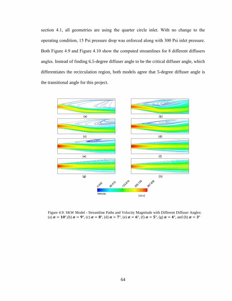
64
section 4.1, all geometries are using the quarter circle inlet. With no change to the
operating condition, 15 Psi pressure drop was enforced along with 300 Psi inlet pressure.
Both Figure 4.9 and Figure 4.10 show the computed streamlines for 8 different diffusers
angles. Instead of finding 6.5-degree diffuser angle to be the critical diffuser angle, which
differentiates the recirculation region, both models agree that 5-degree diffuser angle is
the transitional angle for this project.
Figure 4.9: SKW Model - Streamline Paths and Velocity Magnitude with Different Diffuser Angles:
(a) ,(b) , (c) , (d) , (e) , (f) , (g) , and (h)
[m/s]

65
Figure 4.10: SSTKW Model Streamline Paths and Velocity Magnitude with Different Diffuser
Angles: (a) ,(b) , (c) , (d) , (e) , (f) , (g) , and (h)
Table 4.3: Parametric Study: Single Channel
Turbulence
Model
Angle
(Degree)
Mass
Flow
(g/s)
Max
Channel
Velocity
(m/s)
Max
Inlet
Velocity
(m/s)
Max Mid-
Channel
Velocity
(m/s)
Average
Mid-Channel
Velocity
(m/s)
SKW 10 1.67 258.5 69.1 237.0 177.2
SKW 9 1.68 261.7 69.3 238.0 178.8
SKW 8 1.71 261.4 69.3 239.1 178.9
SKW 7 1.73 263.1 69.4 239.3 179.6
SKW 6 1.75 265.1 69.4 240.2 179.6
SKW 5 1.79 267.2 69.5 240.5 180.1
SKW 4 1.79 267.6 70.1 242.2 181.7
SKW 3 1.77 266.3 69.7 241.5 180.7
SSTKW 10 1.94 269.3 75.82 268.5 193.4
SSTKW 9 1.94 270.5 76.18 269.7 194.3
[m/s]

66
Turbulence
Model
Angle
(Degree)
Mass
Flow
(g/s)
Max
Channel
Velocity
(m/s)
Max
Inlet
Velocity
(m/s)
Max Mid-
Channel
Velocity
(m/s)
Average
Mid-Channel
Velocity
(m/s)
SSTKW 8 1.98 275.1 77.56 274.4 198.0
SSTKW 7 2.00 278.2 78.42 277.4 200.4
SSTKW 6 2.02 282.0 79.43 281.0 203.1
SSTKW 5 2.06 287.1 80.76 285.8 206.6
SSTKW 4 2.06 287.5 80.56 286.0 206.1
SSTKW 3 2.05 285.7 80.11 284.2 204.9
The results from a parametric study for the single channel model are shown in
Table 4.3. The key design factor of mass flow rate was closely monitored. According to
Table 4.3, both models agree that channel mass flow reaches its peak performance when
the geometry of the diffuser (half) angle is tuned in between 4 and 5 degrees. The results
from this table are also corresponded to the outcome shown earlier in Figure 4.10. When
transitional angle 5 degree is reached the maximum mass flow rate can be obtained. Both
results prove the theory when reducing the diffuser angle to a certain degree, the amount
of separation can be limited and, therefore the peak flow performance can be reached.
The trend of mass flow performance versus diffuser angle is shown in Figure 4.11
below. The graph below shows the diffuser geometry is very sensitive for both models; it
directly affects the flow performance of the cooling channel. When the diffuser angle is
less or greater than the critical angles, the flow performance of the channel starts to
decrease.

67
Figure 4.11: Diffuser Angle vs. Mass Flow
The comparison of performances between different diffuser angles can be
constructed in terms of percentage of improvement. In Table 4.4 shows the percentage of
the mass flow improvement for each case compares to the base case with sudden
contraction inlet and sudden expansion outlet.
Note: all diffusers are featuring with quarter circle inlet.
Table 4.4: Mass Flow Improvement for Different Diffusers
Angle
(Degree)
Mass Flow
Improvement (SKW)
Mass Flow
Improvement (SSTKW)
Sudden Contraction and Expansion -- --
10 14.4% 25.2%
9 15.1% 25.2%
8 17.1% 27.7%
7 18.5% 29.0%
6 19.9% 30.3%
5 22.6% 32.9%
4 22.6% 32.9%
3 21.1% 32.3%
3 4 5 6 7 8 9 101.65
1.7
1.75
1.8
1.85
1.9
1.95
2
2.05
Diffuser Angle vs. Mass Flow
Diffuser Angle (Degree)
Ma
ss F
low
Ra
te (
gra
m/s
)
SKW Model
SSTKW Model

68
From all of the comparisons shown in this section, SSTKW model produced
higher value in every category than the SKW model. However, the behaviors of these two
models are very similar. Both models indicated that quarter circle inlet adds more mass
flow performance than the 45° angled inlet, and they both agreed that the transitional
angle for the diffuser is around 5 degree. The final decision of which turbulence model to
use for this project will heavily rely on the experimental data that was gathered at LANL.
4.3 Multi-Channels Study
Evidence from a series of single channel studies has shown that adding a quarter
circle inlet and diffuser outlet improved the mass flow performance in the channel, which
directly improves the heat transfer rate of the cooling channel. Study from section 4.2 has
shown that 4 and 5 degree diffuser (half) angle are the critical angles, which allow
maximum mass flow rate to be reached. From all of this evidence, many of the testing
matrices can be reduced. For instance, for multi-channels study, instead of testing
diffuser (half) angle from 3 to 10 degree, the test was reduced down to 3 to 6 degree. By
doing this process, both computational and experimental expense are reduced by at least
half. In another word, single channel study has helped save both time and money for this
project.
4.3.1 Model Reduction for Multi-Channels Study
Even though the single channel study has helped reduced the testing parameters
by half, modeling the multi-channels model is still computationally intensive. A 27
channels model was constructed to match the experiment that was conducted at LANL.

69
By using multi-channels model with quarter circle inlet and 4 degree diffuser
outlet as an example, to maintain a high quality mesh for selected model an extremely
high value of nodes is required. The mesh matrix for this particular model is shown in
Table 4.5.
With 8 cores processors running on their full speed and 24 GB of physical
memory available for the system, it took almost 72 hours (2,000 iterations) to allow the
model to reach a convergent solution. In addition to the calculation time, an hour of mesh
development time was required before starting the simulation. Figure 4.12 shows a
typical mesh used for the full model.
Table 4.5: Full Model Mesh Matrix
# of Nodes # of
Elements
Orthogonal
Quality
Skewness
13,680,880 12,820,992 0.964 0.110
Figure 4.12: Full Model Mesh (27 Channels with 4 Degree Diffuser)
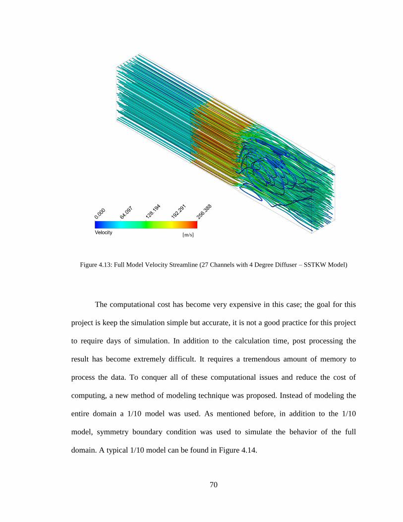
70
Figure 4.13: Full Model Velocity Streamline (27 Channels with 4 Degree Diffuser – SSTKW Model)
The computational cost has become very expensive in this case; the goal for this
project is keep the simulation simple but accurate, it is not a good practice for this project
to require days of simulation. In addition to the calculation time, post processing the
result has become extremely difficult. It requires a tremendous amount of memory to
process the data. To conquer all of these computational issues and reduce the cost of
computing, a new method of modeling technique was proposed. Instead of modeling the
entire domain a 1/10 model was used. As mentioned before, in addition to the 1/10
model, symmetry boundary condition was used to simulate the behavior of the full
domain. A typical 1/10 model can be found in Figure 4.14.
[m/s]
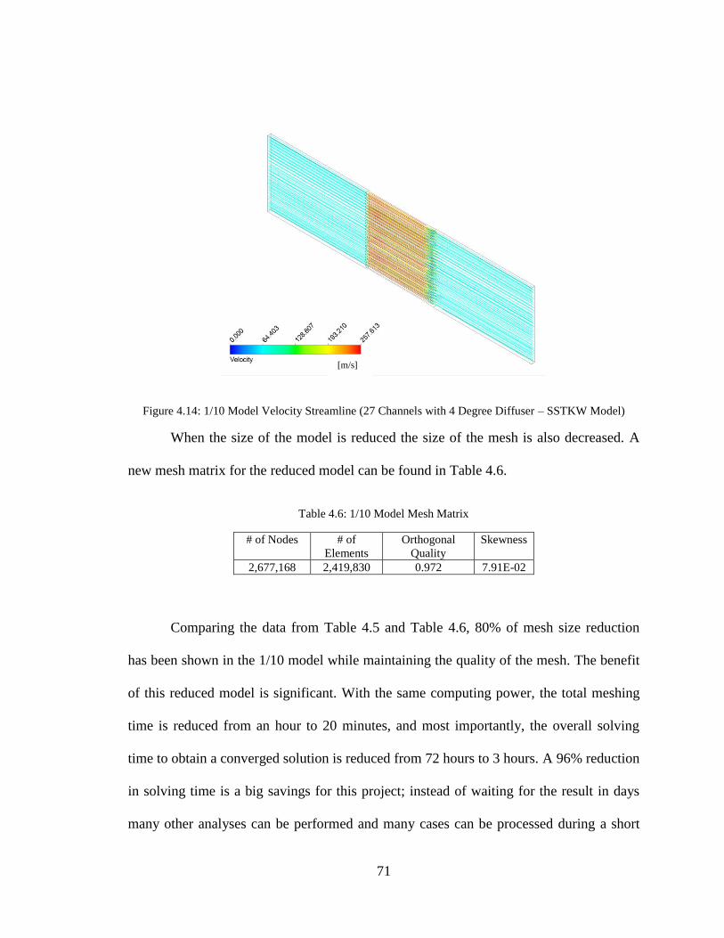
71
Figure 4.14: 1/10 Model Velocity Streamline (27 Channels with 4 Degree Diffuser – SSTKW Model)
When the size of the model is reduced the size of the mesh is also decreased. A
new mesh matrix for the reduced model can be found in Table 4.6.
Table 4.6: 1/10 Model Mesh Matrix
# of Nodes # of
Elements
Orthogonal
Quality
Skewness
2,677,168 2,419,830 0.972 7.91E-02
Comparing the data from Table 4.5 and Table 4.6, 80% of mesh size reduction
has been shown in the 1/10 model while maintaining the quality of the mesh. The benefit
of this reduced model is significant. With the same computing power, the total meshing
time is reduced from an hour to 20 minutes, and most importantly, the overall solving
time to obtain a converged solution is reduced from 72 hours to 3 hours. A 96% reduction
in solving time is a big savings for this project; instead of waiting for the result in days
many other analyses can be performed and many cases can be processed during a short
[m/s]
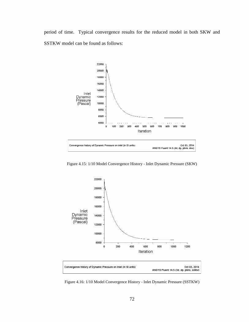
72
period of time. Typical convergence results for the reduced model in both SKW and
SSTKW model can be found as follows:
Figure 4.15: 1/10 Model Convergence History - Inlet Dynamic Pressure (SKW)
Figure 4.16: 1/10 Model Convergence History - Inlet Dynamic Pressure (SSTKW)

73
Figure 4.17: 1/10 Model Convergence History - Inlet Velocity Magnitude (SKW)
Figure 4.18: 1/10 Model Convergence History - Inlet Velocity Magnitude (SSTKW)
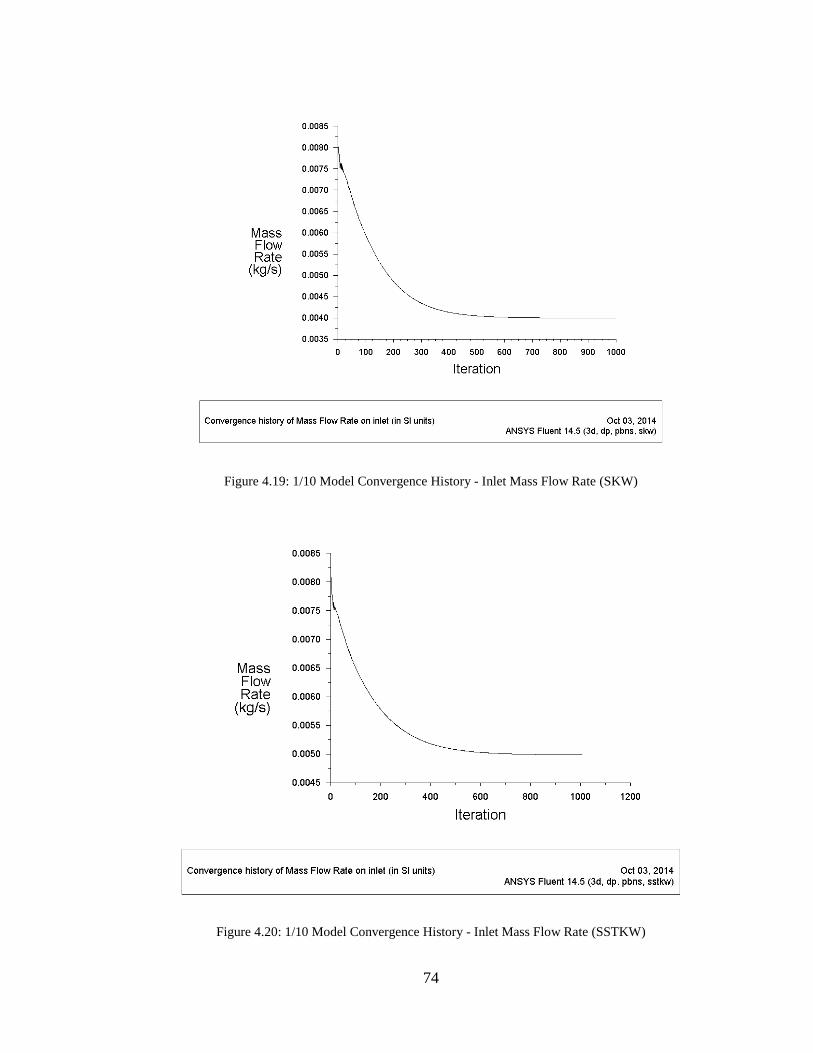
74
Figure 4.19: 1/10 Model Convergence History - Inlet Mass Flow Rate (SKW)
Figure 4.20: 1/10 Model Convergence History - Inlet Mass Flow Rate (SSTKW)

75
From the convergence results shown above, with the 1/10 model, both turbulence
models can provide a stable solution in a short period of time. As expected from the
previous study. The SSTKW model will always produce a higher value in every
catogories that have been compared than the SKW model in every case that has been
compared. The decision on the choice of the turbulence model will depend on how well
the model matches the experimental data. Both turbulence models will be compared
directly to the experimental data collected at LANL in the next chapter. A final decision
on the turbuence model will be made based on the accuracy of the model for this project.
76
Chapter 5 – Validation Analysis
The aim of this chapter is to perform the V&V analysis to make sure about this
CFD analysis. The criteria of V&V have perspective on the base of ASME and AIAA
standard codes. Verification is the process of assessing software correctness and also the
numerical accuracy of the solution for a mathematical model and Validation is defined as
the process of evaluation of the physical accuracy of a mathematical model based on
comparisons between the computational results and the experimental data. [22] To assess
validation an experimental analysis was performed as mentioned earlier, an in-house
experiment at LANL. Based on the early CFD result, many of the design parameters were
finalized. A quarter circle inlet and diffuser outlet were decided for this project. Adding
both features to the existing design has significantly improved the mass flow rate in the
target cooling channels, which will directly increase the heat transfer ability of the
system. From the single channel study, a decision was made to reduce the test parameters
to half and only test the diffuser angle near the critical angle (3 to 6 degree half angle).
With all of these decisions, 6 prototypes were computer drafted and machined, and they
are: sudden contraction and expansion, quarter circle inlet and sudden expansion outlet,
and 4 of quarter circle inlet featured with 3 to 6 degree (half angle) diffuser outlet.
5.1 Experiment Setup
Because of the space constraint for the existing test bench at LANL only 27
channels were able to fit in the test section. This is the main reason why only 27 channels
were modeled instead of the entire 82 channels. A typical drawing for the prototype can

77
be found in Figure 5.1. Following the drawing, an actual prototype is shown in both
Figure 5.2 and Figure 5.3.
Figure 5.1: A Typical Design Drawing for Mo99 Project
Figure 5.2: Mo99 Target Prototype Front

78
Figure 5.3: Mo99 Target Prototype Side View
As explained earlier in Chapter 1, section 3, the driving force for the closed loop
helium gas cooling system is a root blower. During the experiment, the blower pushed
helium gas through the test section and a series data were collected from the test section.
A picture shows in Figure 5.4 gives a little detail about the test section.
Figure 5.4: Solidworks Model for Test Section
Mo99 TargetFlow-in Flow-out

79
Pressure drop and mass flow rate were measured in the experiment model as
validation metrics. To properly record the data needed from this experiment, many of
measuring instruments were used. Two of the most important instruments are flow meter
and pressure gauge. A Flow meter was placed upstream of the test section to monitor
flow before entering into the target cooling channels. Three pressure gauges were used in
this experiment to monitor the pressure across the target cooling channels. The actual
placement of the instruments used in this experiment can be found in Figure 5.5 and
Figure 5.6.
Figure 5.5: Experiment Instruments Setup
Figure 5.6: Experiment Target Placement
Flow Meter
Pressure
Gauge
Target Cooling
Channels

80
5.2 Experimental Incident
Like many other experiments, something unexpected happened during this
experiment. An incident occurred when 6 degree diffuser geometry was tested inside of
the test section; it was the very first one to be tested. A structure failure occurred when
high pressure drop (much greater than15 Psi) was introduced to the target cooling
channels. One of the disks completely separated from the holder and ended up inside of
the flowing loop and two additional ones were collapsed to their neighboring disk.
Luckily, all of the valuable data were taken before this incident happened. Evidence from
this incident can be found in the figures below:
Figure 5.7: Experiment Incident - Two Collapsed Disks

81
Figure 5.8: Experiment Incidence – Broken Disks
Since this incident occurred, all other geometries were tested with extreme care.
Pressure drop across the target cooling channels was monitored closely to make sure that
no extreme pressure drop is introduced to the system. Fortunately, with the new test plan,
this incident did not occur for the rest of the test geometries. The incident also indicates
that there is still room for the test piece to be improved, especially on the structure rigidly
side.
5.3 Experimental Result
Many of the design features can be validated in this section, two main results are
processed from this experiment: mass flow rate as a function of pressure drop and
average mass flow rate at the system required operating condition (15 psi pressure drop
across the channels).

82
The pressure drop across the system is caused by the shape of the target cooling
channels traversed by the flow and by the driving pressure at the inlet of the channels. As
discussed before, pressure drop has a direct relationship between entrance and exit losses.
A decision was made in Chapter 4 that to help reduce the loss at entrance and exit, a
quarter circle inlet and diffuser outlet were added. This part of study focused on how a
change in pressure drop changes the mass flow rate of the system.
To achieve different pressure drop values across the channels, a control unit was
used to control the speed of the motor (in Hertz) to vary the torque of the blower. A 5 Hz
increment was used to separate different pressure drops. From the experiment, the
following pressure drops were closely monitored: 2 psi, 5 psi, 10 psi, and 15 psi. A
comparison from the experiment data is provided in Figure 5.9.
Figure 5.9: Experimental Result - Pressure Drop vs. Mass Flow
Note: All diffusers are featured with a quarter circle inlet

83
Table 5.1: Pressure Drop vs. Mass Flow – Geometry Comparison
Geometry/Pressure Drop Mass Flow Rate (gram/s)
2 Psi 5 Psi 10 Psi 15 Psi
Sudden Contraction and Expansion 14.8 23.1 30.7 35.4
Quarter Circle Inlet 16.8 26.6 33.2 39.4
3 Degree Diffuser 18.9 27.9 35.8 42.4
4 Degree Diffuser 19.8 28.8 36.1 43.6
5 Degree Diffuser 18.5 27.2 35.1 41.4
6 Degree Diffuser 18.1 26.9 34.7 40.7
Table 5.1 shows the pressure drop vs. mass flow result for proposed geometries
from the experiment. At 15 psi (system operating pressure drop), 4 degree diffuser
geometry has the best performance on mass flow, which corresponds to the single
channel study shown earlier. To see how much improvement each geometry has
contributed, Table 5.2 was created to show the comparison.
Table 5.2: Mass Flow Percentage Improvement
Geometry/Pressure Drop Mass Flow Improvement
2 Psi 5 Psi 10 Psi 15 Psi
Sudden Contraction and Expansion -- -- -- --
Quarter Circle Inlet 13.5% 15.2% 8.14% 11.3%
3 Degree Diffuser 27.7% 20.8% 16.6% 19.8%
4 Degree Diffuser 33.8% 24.7% 17.6% 23.2%
5 Degree Diffuser 25.0% 17.7% 14.3% 16.9%
6 Degree Diffuser 22.3% 16.5% 13.0% 15.0%
Use sudden contraction inlet and sudden expansion outlet geometry as the base
model; Table 5.2 shows that in every pressure drop monitored during the experiment, 4

84
degree diffuser geometry has always provided the highest improvement on mass flow
rate. Table 5.2 has also indicated that just adding the quarter circle itself at inlet (without
diffuser outlet) will improve the mass flow rate by 11.3% at the system operating
pressure drop (15 psi). Use 4 degree diffuser as an example, adding a 4 degree diffuser on
top of quarter circle inlet the mass flow rate increases to 23.2%. In another word, 11.9%
improvement in mass flow was added to the system by simply adding 4 degree diffuser
geometry.
Information shown in Table 5.2 can also be transformed into another form of
relation: mass flow as a function of diffuser angle (@15 Psi pressure drop) (see Figure
5.10).
Figure 5.10: Diffuser Angle vs. Mass Flow – Experimental Data (@15 Psi)
3 3.5 4 4.5 5 5.5 640.5
41
41.5
42
42.5
43
43.5
44
Diffuser Angle vs. Mass FlowExperimental Data (@15 Psi)
Diffuser Angle (Degree)
Mass F
low
Rate
(g
ram
/s)

85
5.4 Result and Discussion
In this section, both SKW and SSTKW models results will be evaluated and
compared to the experimental data gathered in this chapter. Early study results from
single channel model shown that both SKW and SSTKW models are good candidates to
predict the right physics for this project. However, the best way to determine the final
turbulence model is to compare them directly to the experimental data. Figure 5.11 -
Figure 5.22 present the streamline contour plots for each computational analysis.
Starting from the sudden contraction and expansion case, both models have
shown a great flow disturbance near the outlet region, which slows down the overall
flow. For this particular geometry (sudden contraction and expansion), two models have
shown different behaviors on the flow velocity distribution. For SSTKW model shown in
Figure 5.11, a group of high velocity flow was concentrated near the inlet region and
quickly dissipating in a short distance. On the other hand, the SKW model has shown a
completely different behavior than the SSTKW model in this case. The SKW model has
shown a more even flow distribution than the SSTKW model. However, the average flow
rate for the SSTKW model is still higher than the SKW model. Evidence from both cases
shows that by adding the quarter circle inlet and diffuser outlet, the velocity magnitude
increases and the regions of flow disturbance are significantly reduced, which increases
the cooling performance of the system. Evidence has also shown that as the angle of the
diffuser starts to increase the flow disturbance starts to gain back its stage.

86
Figure 5.11: Velocity Streamline - Sudden Contraction and Expansion (SSTKW Model)
Figure 5.12: Velocity Streamline - Sudden Contraction and Expansion (SKW Model)
[m/s]
[m/s]

87
Figure 5.13: Velocity Streamline - Quarter Circle Inlet (SSTKW Model)
Figure 5.14: Velocity Streamline - Quarter Circle Inlet (SKW Model)
[m/s]
[m/s]

88
Figure 5.15: Velocity Streamline - 3 Degree Diffuser (SSTKW Model)
Figure 5.16: Velocity Streamline - 3 Degree Diffuser (SKW Model)
[m/s]
[m/s]

89
Figure 5.17: Velocity Streamline - 4 Degree Diffuser (SSTKW Model)
Figure 5.18: Velocity Streamline - 4 Degree Diffuser (SKW Model)
[m/s]
[m/s]

90
Figure 5.19: Velocity Streamline - 5 Degree Diffuser (SSTKW Model)
Figure 5.20: Velocity Streamline - 5 Degree Diffuser (SKW Model)
[m/s]
[m/s]
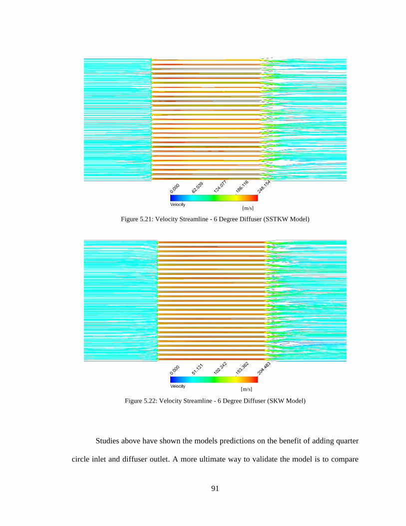
91
Figure 5.21: Velocity Streamline - 6 Degree Diffuser (SSTKW Model)
Figure 5.22: Velocity Streamline - 6 Degree Diffuser (SKW Model)
Studies above have shown the models predictions on the benefit of adding quarter
circle inlet and diffuser outlet. A more ultimate way to validate the model is to compare
[m/s]
[m/s]

92
the model result directly to experimental data. A system matrix is created to compare all
models and data side by side. A relative error was also evaluated by using the
experimental data as the base case. The comparison result can be found in Table 5.3
shown below.
Table 5.3: Results Comparison - Models vs. Experimental Data (@15 Psi Pressure Drop)
Geometry/Data
Mass Flow Rate (gram/s) SSTKW
Error
SKW
Error SSTKW
Model
SKW
Model
Experiment
Sudden Contraction and Expansion 35.1 28.3 35.4 0.847% 20.1%
Quarter Circle Inlet 39.1 35.0 39.4 0.761% 11.2%
3 Degree Diffuser 49.8 41.1 42.4 17.5% 3.07%
4 Degree Diffuser 50.2 42.8 43.6 15.1% 1.83%
5 Degree Diffuser 49.2 40.9 41.4 18.8% 1.21%
6 Degree Diffuser 48.4 39.6 40.7 18.9% 2.70%
From the comparison shown in Table 5.3 some interesting results were found. For
SSTKW model, it shows its strong ability of predicting the results for both sudden
contraction and expansion and quarter circle inlet cases. The relative error produced from
SSTKW model for these two cases were less than 1%. However, SSTKW did not
perform so well on the diffuser cases. It shows a 15-19% error margin when predicting
the diffuser geometries. On the other hand, SKW model behaved the opposite way than
SSTKW model. For the sudden contraction and expansion and quarter circle inlet cases,
SKW model leaves 11-20% error for its prediction. However, SKW model shows a
strong performance on predicting the diffuser cases. Only 1-3% error was shown when
using the SKW model.

93
The advantages and disadvantages of both turbulence models have been obtained by
above mentioned analysis. The ultimate question that needs to be answered now is which
model is more useful for this project. The main focus of this project is to predict the right
physics for the new geometry designs. When carefully evaluating the values of both
models, evidence indicates that SKW model is the better candidate than the SSTKW
model for this project. SKW model shows its strong side of predicting the diffuser
geometries, which will eventually be used in the production. In Figure 5.23 shows the
direct comparison between the experimental data and the two models.
Figure 5.23: Final Result Comparison – Models vs. Experimental Data
From the result shown in Figure 5.23, clearly the SKW model has the ability of
predicting the right result for the diffuser geometries at the required operating condition.
3 3.5 4 4.5 5 5.5 638
40
42
44
46
48
50
52
Diffuser Angle vs. Mass Flow
Result Comparison (@15 Psi)
Diffuser Angle (Degree)
Mass F
low
Rate
(g
ram
/s)
Experimental Data
SKW Model
SSTKW Model

94
To ensure that the decision on the turbulence model is reliable a further analysis was
conducted to make sure that the right turbulence model was chosen.
Early in this chapter, a plot was generated from the experimental data to show the
relation between pressure drop and mass flow rate for different geometries (Figure 5.9).
Since both experimental data and CFD model show that 4 degree diffuser design
performs the best on mass flow rate, 4 degree diffuser design was used as a test case to
help determine stability of the SKW model. In addition to the 15 Psi pressure drop
operating condition, 3 more operating conditions were ran for this test and they are: 2 Psi,
5 Psi, and 10 Psi. The comparison result is shown in Figure 5.24.
Figure 5.24: Mass Flow as a Function of Pressure Drop
Experimental Data vs. SKW Model (4 Degree Diffuser Design)
15 20 25 30 35 40 452
4
6
8
10
12
14
16
18
Pressure Drop vs. Mass FlowExperimental Data vs. SKW Model
Mass Flow (gram/s)
Pre
ssu
re D
rop
(P
si)
Experimental Data
SKW Model

95
Based on the result shown in Figure 5.24, once again the SKW model has proven
its strong ability of predicting the right behavior of the diffuser geometries for this
project.
The performed assessment analysis shows that the SKW model is truly the right
candidate for the 99
Mo project. Both CFD model and experimental data are showing that
4 degree diffuser design is best design compared to all other proposed designs. A
maximum mass flow was achieved by using this geometry.
96
Chapter 6 – Conclusions and Recommendations
6.1 Conclusions
The turbulent flow through a cooling channel featuring different inlet and diffuser
outlet designs has been investigated using the computational fluid dynamics software
ANSYS FLUENT 14.5. The built-in standard model was validated with the
experiment conducted at LANL. A very good agreement between the simulation result
and the experimental data was shown in the early chapters. By using the single channel
model shown in Figure 4.9 and Figure 4.10, a correlation between recirculation and
diffuser angle was found for this particular project. From single channel study, there will
not be any recirculation region when diffuser angle is equal to, or less than 5-degree. This
correlation later proved that 5-degree diffuser angle is the critical angle, which is the
turning point that affected the overall performance of the flow.
Two inlet features were proposed and compared. Quarter circle inlet was chosen
over the 45° angled inlet due to its ability of reducing the head loss around the inlet
section. Just by adding the quarter circle inlet itself, 12.3% of mass flow improvement
was added to the system compared to the base case design (sudden contraction and
expansion).
In addition to the inlet geometry, a diffuser design was added to the downstream
of the target cooling channel. Evidence from both experiment and CFD model have
shown that diffuser design is an efficient mechanism for decelerating the flow to prevent
disturbance flow and at the same time recovering the dynamic pressure smoothly.

97
Not like the single channel study, multi-channels study was more complex. As
mentioned earlier, the ideal case shown in single channel study could not be reproduced
in the multi-channels case. There was always separation or disturbance flow in the
channel. However, there was one phenomenon that occurred in both single channel and
multi-channel studies. Both studies agreed that by decreasing the diffuser angle to a
certain degree, separation will decrease but mass flow will increase. Proof for this
phenomenon can be found from Figure 5.11 to Figure 5.22 from the multi-channels
study.
Before conducting the multi-channels study, results gathered from single channel
study were used to reduce the test parameters for both CFD model and experiment.
Significant amounts of testing time were saved from this process.
Model validation and verification was crucial for this project. Starting from the
beginning, a benchmark test was conducted by using the experimental data from Buice
[19], initial result shown in Figure 3.7 indicated that both SKW and SSTKW models are
the good candidates for this project. However, by comparing the results from both models
to the experimental data, a final decision was made that the SKW model is the better
candidate than the SSTKW model for this project. Besides comparing model result to the
experimental data, mesh independency was also studied to prevent deficiency from the
model. A series of mesh matrix were tested and many methods were used to ensure the
stability of the model. Evidence for model stability can be found throughout Chapter 3.
Finally, a new geometry design was finalized from this study. Both experimental
data and CFD model agreed that quarter circle inlet and 4 degree diffuser design is the

98
best combination for this project with the mission of improving heat transfer performance
for the 99
Mo target cooling loop. 4 degree diffuser design showed less separation and
higher mass flow rate than other diffuser designs.
The same methodology used in this project can be applied to many other channel
flow design project that involves flow separation and diffusers. Finding the correlation
between diffuser angle and recirculation flow for the design is critical. By doing the
procedures described in this project, one’s designing time can be significantly reduced
when it comes to optimizing the performance of a channel flow.
6.2 Suggestions for Future Work
There are many areas that can be improved for this project. As mentioned in
Chapter 5 section 5.2, an incident occurred during the experiment. Because of this
incident all other test pieces were treated with extreme care during the experiment. For
the future work, design and machine more rigid test pieces than the current ones so that a
higher pressure drop can be tested.
Another big suggestion for this project is to conduct a particle image velocimetry
(PIV) test. Due to the time constraint this part of test could not be completed. If this test
was conducted many interesting phenomena can be discovered visually from the
experiment. For instance, the wall effects, the stagnation point at the entrance, and the
separation region near the diffuser. A visual comparison between CFD model and
experiment can also be performed.
The final suggestion for the future work is to conduct thermal-hydraulics
modeling. The reason why thermal-hydraulics model was not constructed for this project

99
was because there has not been an easy to conduct experiment to validate the model.
Without using the real electron beam from the actual accelerator, heating the targets has
become a very difficult task. Maybe in the near future there is an inexpensive method to
heat up all 25 disks in the test section and have a Gaussian distribution of the heat flux
applied to the test piece.

100
References
[1] World Nuclear Association, 2012, “Radioisotopes in edicine”, from
http://www.world-nuclear.org/info/inf55.html.
[2] Dale, G. E., Chemerisov, S. D., Vandegrift, G. F., Woloshun, K. A., Kelsey, C. T.
IV, Tkac, P., Makarashvili, V., Jonah, C. D., Olivas, E. R., Hurtle, K. P., Romero,
F. P., Dalmas, D. A., Holloway, M. A., Harvey, J. T., 2012, “Design and
Experimental Activities Supporting Commercial U. S. Electron Accelerator
Production of Mo-99”, LA-UR-12-23810, Los Alamos National Laboratory, Los
Alamos, New Mexico.
[3] D.R. cAlister and E.P. Horwitz, “Automated two column generator systems for
medical radionuclides.” Appl Radiat Isot., 67, pp. 1985-91, 2009.
[4] Division of Environmental Health, Office of Radiation Protection, July 2002,
“Technetium-99m (99m
Tc)”, Fact Sheet 320-083, Washington State Department of
Health.
[5] U.S. EPA OSWER, “EPA Facts About Technetium-99: July, 2002”, (2002): n.
pag. Print.
[6] Lyra M., Charalambatou P., Roussou E., Fytros S., Baka I.,March 2011,
“Alternative production methods to face global molybdenum-99 supply shortage”,
Hellenic Journal of Nuclear Medicine., 14(1), pp 49-55, 2011.
[7] Petersen Vroman P. 2014, “Helium-Cooling Loop for a Molybdenum-99
Accelerator-Production System”. Master Thesis, Bradley University, 2014.

101
[8] Zucrow, M. J., Hoffman, J. D., Gas Dynamics Volume 1, John Wiley & Sons,
Inc., Hoboken, NJ, Chap. 6.
[9] Anderson, John David. Computational Fluid Dynamics: The Basics with
Applications. New York: McGraw-Hill, 1995.
[10] Currie, Iain G. Fundamental Mechanics of Fluids. Boca Raton, FL: Taylor &
Francis, 2013.
[11] Munson, Bruce Roy, T. H. Okiishi, and Wade W. Huebsch. Fundamentals of
Fluid Mechanics Sixth Edition. Hoboken, NJ: J. Wiley & Sons, 2009. Print. Chap
1, Chap 3, Chap 7.
[12] Obi S, Aoki K, Masuda S, “Experimental and computational study of turbulent
separating flow in an asymmetric plane diffuser”. In: Ninth symposium on
turbulent shear flows, Kyoto, Japan; 16-19 August 1993. p. 305-1-4.
[13] Kaltenbach, H-J 1994, Large-eddy simulation of flow through a plane,
asymmetric diffuser. Annual Research Briefs-1994, Center for Turbulence
Research, Stan- ford Univ./NASA Ames, pp. 175-184.
[14] D. C.Wilcox. Turbulence Modeling for CFD. DCW In- dustries, Inc. La Canada,
California. 1998.
[15] F. R. Menter. Review of the SST Turbulence Model Experience from an Industrial
Perspective. International Journal of Computational Fluid Dynamics. Volume 23,
Issue 4.. 2009.
[16] B. E. Launder and D. B. Spalding. “The Numerical Computation of Turbulent
102
Flow”. Computer Methods in Applied Mechanics and Engineering. 3. 269-289.
1974.
[17] S.M. El-Behery, M. Hamed A comparative study of turbulence models
performance for separating flow in a planar asymmetric diffuser Computer and
Fluids, 44 (2011), pp. 248-257
[18] ANSYS FLUENT Theory Guide 14.5. Canonsburg, (PA): ANSYS Incorporated;
2012.
[19] Buice, C.U. and Eaton, J.K., Experimental Investigation of Flow through an
Asymmetric Plane Diffuser, Dept. of Mech. Eng, Stanford University, TSD-107
(1997)
[20] H. Lan, B.F Armaly, and J.A Drallmeier. Turbulent Forced Convection in a Plane
Asymmetric Diffuser: Effect of Diffuser Angle. Journal of Heat Transfer, Vol.
131/071702
[21] Berdanier, Reid A. Turbulent Flow through an Asymmetric Plane Diffuser.
Thesis. Purdue University, 2011
[22] Oberkampf, William L., and Christopher J. Roy. Verification and Validation in
Scientific Computing. New York: Cambridge UP, 2010.