Embed Size (px)
Citation preview

AD-AO08 590
CORRELATION OF FATIGUE DATA FOR ALUMINUM AIRCRAFTWING AND TAIL STRUCTURES
R. Hangartner
National Aeronautical Establishment
Prepared for:
National Research Council of Canada
December 1974
DISTRIBUTED BY:
National Technical Information ServiceU. S. DEPARTMENT OF COMMERCE
II

* ./ National Research Conseil nationalU Council Canada de recherches Canada
CORRELATION
OF FATIGUE DATA
FOR ALUMINUM AIRCRAFT
WING AND TAIL STRUCTURES
BY
R. HANGARTNER
NATIONAL AERONAUTICAL- ESTABLISHMENT
DDC
OTTAWA MAY 9 1975
DECEMBER 1974 [rUL i-ePJ-f
loproduced by DNATIONAL TECHNICALINFORMATION SERVICE
US Dopattmo.t of ComemerceSpringfield, VA. 22151 AERONAUT ICAL
NRC NO. 14555 REPORT
ISSN oo77-554i DISTRIBUT1oN TATEM.ENTA R-582Approved for public release;
Distribution Unlimited
r\ , . .

CORRELATION OF FATIGUE DATA
FOR ALUMINUM AIRCRAFT WING
AND TAIL STRUCTURES
CORRELATION ENTRE LES DONNEES DE FATIGUE
RELATIVES AUX STRUCTURES D'AILE ET D'EMPENNAGE D'AVION
EN-ALUMINIUM
Vby/par
R. HANGARTNER
DDC
MA Y 9 1.975j~
• [3
A.H. Hall, Head/Chef
Structures and Materials Laboratory/ F.R. ThurstonLaboratoire des structures et materiaux Director/Directeur
D[STBIBUTION STATEMENT-A
Approved for public releaso;Distribution Unlimited I

SUMMARY
S-N curves are derived for aluminum wing and tail structures byfitting various regression models to, 246 full-scale constant-amplitude fatiguetest results from twelve types of aircraft structures. The derived curves weretested by comparing the predicted lives with actual. test results of variousaircraft structures fatigue tested to variable-amplitude loads spectra. Morereliable predictions resulted from these derived S-N curves than from existingS-N curves.
RESUME
Les courbes de fatigue relatives aux structures d'aile et d'empennagesont obtenues grdce l'6tude, au moyen de modales bas6s sur la m6thode deregression, des 246 r~sultats des essais de fatigue en vraie grandeur, et ' ampli-tude constante, entrepris sur douze types de cellules d'avion. Les courbesobtenues ont 6t6 contrbl~es en comparant les dures de vie pr6vues auxr6sultats des essais de fatigue r6els effectu6s, suivant un spectre de chargesd'amplitude variable, sur diff~rentes cellules d'avion. Ces nouvelles courbespermettent des predictions plus fiables qu'avec les courbes de fatigue exis;tantes.

TABLE OF CONTENTS
Page
SUMMARY ................................................................................................................. .(iii)
TABLES ................................................................................................................... (v)
ILLUSTRATIONS ....................................................................................................... (v)
APPENDICES ............................................................................................................. (vi)
ABBREVIATIONS ...................................................................................................... (vi)
NOMENCLATURE ..................................................................................................... (vi)
1.0 INTRODUCTION ........................................................................................................ I
2.0 S-N CURVES DERIVED FROM FULL-SCALE STRUCTURES ................................ 1
3.0 CONSTANT-AMPLITUDE FATIGUE TEST RESULTS ................... ...................... 2
3.1 Definitions, Assumptions and Other Relevant Information .................................. 23.2 General Comments on Fatigue Tests .................................................................. 3
4.0 ANALYSIS OF RESULTS .......................................................................................... 3
4.1 Mathematical Models .......................................................................................... 3
4.1.1 Log N Versus Log sa Curves ................................................................. 34.1.2 Log N:Versus Sa Curves ........................................................................... 4
4.2 Residuals ............................................................................................................. 5
5.0 COMPARISON OF S-N CURVES ............................................................................... 5
6.0 SCATTER IN CONSTANT-AMPLITUDE FATIGUE DATA .................................... 6
6.1 Scatter Within a Group of Similar Structures ...................................................... 66.2 Scatter Due to Different Types of Structures ...................................................... 6
7.0 LIFE PREDICTIONS USING VARIOUS S-N CURVES AND RELIABILITYOF PREDICTIONS ............................................................................. 7
7.1 Lives Predicted by Various S-N Curves ............................................................... . 77.2 Reliability of Predictions .................................................................................... 8
8.0 CONCLUSIONS .......................................................................................................... 9
9.0 REFERENCES .......................................................................................................... 9
(iv)
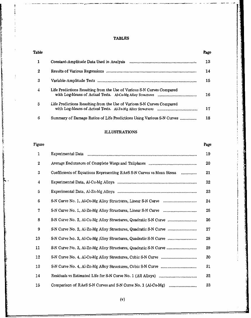
TABLES
Table Page
1 Constant-Amplitude Data Used in Analysis ......................................................... 13
2 Results of Various Regressions ................................................................................ 14
3 Variable-Amplitude Tests ......................................................................................... 15
4 Life Predictions Resulting from the Use of Various S-N Curves Comparedwith Log-Means of Actual Tests. Al-Cu-Mg Alloy Structures ................................... 16
5 Life Predictions Resulting from the Use of Various S-N Curves Comparedwith Log-Means of Actual Tests. AI-Zn-Mg Alloy Structures .................................... 17
6 Summary of Damage Ratios of Life Predictions Using Various S-N Curves .............. 18
ILLUSTRATIONS
Figure Page
1 Experim ental Data ................................................................................................. . 19
2 Average Endurances of Complete Wings and Tailplanes .......................................... 20
3 Coefficients of Equations Representing RAeS S-N Curves vs Mean Stress .............. 21
4 Experimental Data, Al-Cu-Mg Alloys ....................................................................... 22
5 Experimental Data, AI-Zn-Mg Alloys ....................................................................... 23
6 S-N Curve No. 1, Al-Cu-Mg Alloy Structures, Linear S-N Curve .............................. 24
7 S-N Curve No. 1, Al-Zn-Mg Alloy Structures, Linear S-N Curve ............................. 25
8 S-N Curve No. 2, Al-Cu-Mg Alloy Structures, Quadratic S-N Curve ......................... 26
9 S-N Curve No. 2, Al-Zn-Mg Alloy Structures, Quadratic S-N Curve ................ 27
10 S-N Curve No. 3, Al-Cu-Mg Alloy Structures, Quadratic S-N Curve ......................... 28
11 S-N Curve No. 3, Al-Zn-Mg Alloy Structures, Quadratic S-N Curve .......................... 29
12 S-N Curve No. 4, Al-Cu-Mg Alloy Structures, Cubic S-N Curve ........................... 30
13 S-N Curve No. 4, Al-Zn-Mg Alloy Structures, Cubic S-N Curve ............................... 31
14 Residuals vs Estimated Life for S-N Curve No. 1 (All Alloys) ................................. 32
15 Comparison of RAeS S-N Curves and S-N Curve No. 1 (Al-Cu-Mg) ........................ 33
(v)

ILLUSTRATIONS (Cont'd)
Figure Page
16 Actual vs Predicted Lives for S-N Curve No. 1 (All Alloys) ........................................ 34
17 Probability of Damage Ratios Being Exceeded for S-N Curve No. 1 andRAeS S-N Curves ................................................................................................... 35
18 Probability of Damage Ratios Being Exceeded for S-N Curve No. 2 andRAeS S-N Curves ................................................................................................... 36
19 Probability of Damage Ratios Being Exceeded for S-N Curve No. 3 andRAeS S-N Curves ................................................................................................... 37
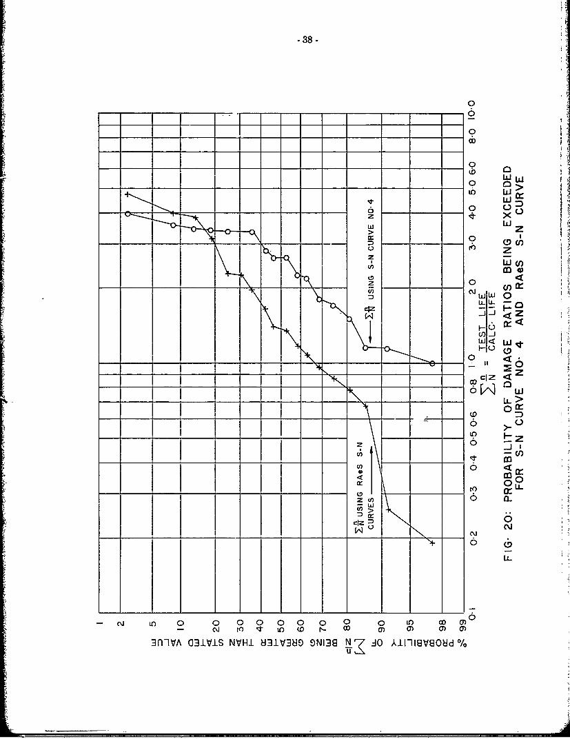
20 Probability of Damage Ratios Being Exceeded for S-N Curve No. 4 andRA eS S-N Curves ................................................................................................... 38
n21 Comparison of 1 - Values for Various S-N Curves at Equal Reliabilities ................... 39
N
APPENDICES
Appendix Page
I Methods for Interpolating Between the RAeS S-N Curves ................................. 41
II Computer Output of Typical Life Calculation ................................................... 43
ABBREVIATIONS
ESDU Engineering Sciences Data Unit
ksi kips per square inch
RAeS Royal Aeronautical Society
NOMENCLATURE
A, B, C, D coefficients
bl, b2, ... bi coefficients
f, f, ... fi general functions
M material parameter in regression equation
n, N number of cycles
(vi)

NOMENCLATURE (Cont'd)
S..,S'It alternating stress (ksi)
sillSillcan mean stress (ksi)
U standard deviation
(vii)

-1-
CORRELATION OF FATIGUE DATA FOR ALUMINUM
AIRCRAFT WING AND TAIL STRUCTURES*
1.0 INTRODUCTION
This document establishes more consistent S-N curves for the fatigue life prediction of alu-minum aircraft wing structures than the presently available RAeS-ESDU S-N curves for "Typical Wingsand Tailplanes" (Ref. 1).
Constant-amplitude fatigue testresults from 246 aircraft wings and tails from twelve aircrafttypes were pooled and various regression models were fitted in order to obtain mathematical expressionsfor sets of S-N curves.
These curves and the existing RAeS-ESDU curves were then used to predict the lives ofvariable-amplitude tests and the calculated lives were compared with the actual test results.
In the life calculations the method of linear cumulative damge (Palmgren-Miner Rule) wasutilized.
2.0 S-N CURVES DERIVED FROM FULL-SCALE STRUCTURES
When estimating the life of a-wing structure when structural details and an extensive stressanalysis of the wing are not available it is normally better to use S-N curves derived from built-up struc-tures than those derived from notched material coupons. Reasons for this include the fact that thereis no fretting in a simple 3pecimen and a simple specimen has only one load path whereas many struc-tures are redundant.
RAeS-ESDU published a set of S-N curves derived from 137 full-scale fatigue tests on wingsand tailplanes of various aluminum alloy aircraft structures (Ref. 1). These data and curves are re-produced in Figures 1 and 2.
Upon inspection of Figure 2 it is noticed that the curves do not follow the same generaltrend. It is easily seen that the line for five ksi mean stress does not follow the pattern of the lines forthe other mean stresses. It is understood that the curves were drawn by "eye" and to illustrate thisinconsistency the slopes and intercepts of the lines were plotted.
Straight lines on log-log plots can be expressed by the equations
log,0 N = A + Blog, 0 Sa
or log, 0 S, = C + Dlog 10 N
The coefficients A, B, C and D were calculated for the lines shown in Figure 2 and theirvalues were plotted versus mean stress in the graphs shown in Figure 3. The discontinuities in thecurves tend to confirm that a mathematical analysis was not performed on the data.
Because of this and together with the fact that many additional data are now available itwas decided to re-analyze the data and to include as many new data as could be obtained.
• The work in this report is a summary of the author's Master's Thesis submitted at the Universityof Waterloo, Waterloo, Ontario, Canada.

-2-
3.0 CONSTANT-AMPLITUDE FATIGUE TEST RESULTS
In a literature search approximately 400 full-scale test results werelocated; however, only246 were used in the analysis. The criteria for data selection were as follows:
1) The nominal stresses in the failure regions were well defined.
2) Only data from constant-amplitude tests were used in the analysis.
3) All data used had fatigue lives in the range 103 < N < 10 7 cycles.
4) All data used were from tests conducted at room temperature.
Table 1 lists the types of structures, the number of results used, and the references fromwhich they were obtained. Reference 16 gives a more detailed list of the test results used in the anal-ysis. The test results are plotted in Figures 4 and 5, these figures showing the test results for theAl-Cu-Mg alloys (e.g. 2024, and similar alloys) and the Al-Zn-Mg alloys (e.g. 7075) respectively.
3. Definitions, Assumptions, and Other Relevant Information
1. Approximately three-quarters of the structures were manufactured from Al-Cu-Mg alloysand one-quarter of the structures from Al-Zn-Mg alloys. Preliminary analysis showed that alarge diffet1 nce in fatigue life existed between these two types of structures; thus, allowancehad to be made for this in the analysis.
2. Failure was defined as final or catastrophic failure, i.e. the applied load could no longer besupported by the structure. An analysis defining crack initiation as failure would be diffi-cult in that many airframes had some service history before fatigue testing and a portion ofthese aircraft already had cracks in fatigue-critical regions.
3. Some of the wings used in the RAeS analysis and also the present analysis wrere not cycledto complete failure. Some probable reasons were:
i) to reduce the time required for testing,
ii) inability of the test rig to cycle only one half of a wing, and
iii) to avoid damage to the test apparatus.
The lives of these wings were estimated by their respective researchers. These estimates werebased upon the propagation rates of fatigue cracks in the specimen under consideration. Com-parison with lives and crack propagation rates were also available from other specimens testedat the same load range.
4. The stresses used in the analysis were nominal or gross-section stresses in or near the fatigue-critical region. The actual stress in the initiation area was usually not known unless deter-mined by sophisticated methods of stress analysis.
5. In general, two types of loading rigs, hydraulic and vibration, were used for fatigue testing.Ford and Payne (Ref. 4) found that in their tests on Mustang wings there was no significantdifference in the variance and mean of the lives of two sets of several wings tested at thesame load level in different loading rigs, one a hydraulic type and one a vibration type.
6. The precision with which loads were controlled in the various fatigue tests is unknown asnot all the references discussed details of the testing methods, equipment, calibrationprocedures, and methods of load monitoring. This fact does add an unknown quantity ofscatter to the results of the analysis.

-3-
7. It was assumed that the geometries of these various structures were similar in that being full-scale structures they all contained similar stress conenti-ations. such as holes, rivets, bolts,hydraulic fittings, changes in section, cutouts, stiffeners, reinforcements, surface attachments,etc., all of which are potential sources of crack initiation.
3.2 Gt.aeral Comments on Fatigue -Tests
Data from many structures found in the references could not be used in the analysis becauseof a lack of stress data for the failure locations. Probably some of this information was not publishedat the time of the tests for security reasons. Also, even though some references to structural fatiguetests prior to the 1950's were found, most reports from this era were either no longer in existence ornot easily obtained. Other test results are probably available from the aircraft industry, such as resultsof tests that were published for internal use and not widely circulated.
4.0 ANALYSIS OF RESULTS
In the present analysis the fatigue life has been assumed to be a function of applied loadsand the material (in this case either Al-Cu-Mg or AI-Zn-Mg alloy). The loads on a structure can bereduced to the form Smean ± Salt; thus, for our purposes the fatigue life can be represented by
N = f (Sm ean, Salt, Material)
4.1 Mathematical Models
Four mathematical models were fitted to the data using the method of least-squares. Themodels proposed were of the following form:
logl 0 N = f (Sm) + f2 (Sa) + f3 (M)
The various regression models were compared using statistics such as standard error of esti-mate and coefficient of correlation.
4.1.1 Log N Versus Log Sa Curves
The first model was:
log, 0 N b, + b2 Sm + b3 Sm + b4 m) + b5 log1 0 Sa
where Sm and Sa are in ksi. In this model fl is a cubic polynomial in mean stress, f2 is log-linear inalternating stress, and f 3 was zero as at this stage it was not yet realized that structures manufacturedfrom different aluminum alloys would have significantly different lives. This model yielded a familyof straight lines on log-log (log N vs. log Sa) paper.
In order to reduce the number of parameters, the cubic polynomial fI for interpolatingmean stress was replaced by a logarithmic function, log, 0 (Sm + 5). An arbitrary constant of 5 wasadded to the mean stress so that the expression would be valid for Sm = 0 and also could be extra-polated to mean stresses slightly less than zero if desired.
With the logarithmic interpolation for mean stress a slightly better correlation resulted, theslopes of the lines of the two models differing by less than 0.2% and the lines were almost coincident.Therefore the logarithmic function for the interpolation of mean stress was retained-in all the regressions.

From the results it was also evident, that there were significant differences in the lives ofstructures of the two material types. To account for this a dummy variable for material type was used.
The model then became
log, 0 N = b, + b, log, 0 (Sm + 5) + b3 log, 0 Sa + b4 M (S-NCurve No. 1)
where M = 0 for Al-Cu-Mg Alloys
M = 1 for Al-Zn-Mg Alloys
With the dummy variable, the S-N curves for the two alloys would be of similar shape, onlydisplaced along the log N axis by the value of the coefficient of M (b4 in this case).
Figure 6 shows S-N Curve No. 1 for the Al-Cu-Mg alloy structures and Figure 7 shows S-NCurve No. 1 for the Al-Zn-Mg alloy structures.
In the next regression the term (log 1 0 Sa )2, was added to f,. With this quadratic term, aslightly higher coefficient of correlation was obtained. The model then became
log1 0 N = b1 + b2 log10 (Sm + 5) + b3 log, 0 Sa + b4 (log10 S)2 + b5 M (S-N Curve No. 2)
The resulting S-N curves were a family of parabolas on log-log paper. S-N Curve No. 2 for the Al-Cu-Mgalloy structures is shown in Figure 8 and Figure 9 shows S-N Curve No. 2 for the Al-Zn-Mg alloy struc-tures.
The curves look unusual since they are concave downwards; however, when curves are fittedto experimental data the resulting empirical expressions may "best fit" the data but may not representthe physical process involved. The addition of a cubic term, (log, 0 Sa )3, did not improve the correlation.
4.1.2 Log N Versus Sa Curves
In these regressions f2 was represented by polynomial functions of Sa, rather than log SaThe mean stress was still interpolated logarithmically.
The first model of this set used a quadratic function of Sa for f2 and the expression for theS-N curve thus became
log1 0 N - b, + b2 log1 0 (Sm + 5) + b3 Sa + b4 Sa + b5 M (S-NCurveNo. 3)
The resulting curves were a set of parabolas on semi-log paper. The coefficient of correlationwas slightly less than that obtained with the linear curves of log N versus log Sa.
Figure 10 and Figure 11 show S-N Curve No. 3 for the Al-Cu-Mg and Al-Zn-Mg alloy struc-tures respectively.
Upon studying the figures it is noticed that in the high-alternating-stress low-endurance regionthe curves rise sharply. This is not, of course, representative of typical S-N curves and re-ults from theconstraint of the parabolic fit. Extrapolation of the curves beyond the plotted values would lead toerroneous results.5 :

-5-o
The second model in this set included a cubic term in Sa . Thus, the model became
log, 0 N = b1 + b2 log, 0 (Sm + 5) + b3 Sa + b4 Sa + b5 S " + b6 M (S-N Curve No. 4)
The resulting S-N curves were a set of cubics on semi-log paper. With this regression the co-efficient of correlation was slightly higher than those obtained with the parabolas of log N versus log Sa .
S-N Curve No. 4 for the Al-Cu-Mg and Al-Zn-Mg alloy structures is shown in Figures 12 and13 respectively.
Table 2 lists the coefficients of the parameters and some statistics obtained from the fourregression models.
Further regressions were not attempted as it appeared that all four of these-models yieldedsimilar results and more complex models would only slightly increase the coefficient of correlation.
4.2 Residuals
Residuals are the differences between the actual test results and the predictions from theregression equation.
Figure 14 shows the residuals plotted versus the values predicted by the regression equationfor S-N Curve No. 1.
No abnormality exists if the plotted residuals form a horizontal band, rather than showingsome trend such as increasing or decreasing when plotted versus the predicted value. The points inFigure 14 appear to form a horizontal band in that no other trend is noticed; thus, the least-squaresanalysis would not appear to be violated.
Residual plots forthe other S-N curves are not included as they are~similar. They can befound in Reference 16.
5.0 COMPARISON OF S-N CURVES
The derived Al-Zn-Mg alloy S-N curves cannot be compared with the RAeS curves as all dataused in the RAeS analysis were from Al-Cu-Mg alloy structures; however, the Al-Cu-Mg alloy curves canbe compared.
Figure 15 shows S-N Curve No. 1 for Al-Cu-Mg alloys and the RAeS S-N curves superposed.Comparisons for the other curves are not shown since they are similar.
When comparing the derived Al-Cu-Mg alloy S-N curves with the RAeS curves the followinggeneralities are noticed:
1) They are less conservative at high mean stresses, i.e. greater than 20 ksi.
2) At the lower mean stresses they are.less conservative in the low-endurance high-alternating-stress region.
3) At the lower mean stresses they are more conservative in the high-endurance low-alternating-stress region.

-6-
In conjunction with the above three statements the following should also be taken into con-sideration:
1) Mean stresses greater than,20 ksi are rare in practice.
2) The frequency of loads in-the low-endurance high-alternating-stress region is low; thus, theireffect on fatigue life (using a linear damage rule) is negligible.
3) The frequency of loads in the high-endurance low-alternating-stress region is high; therefore,the fatigue life can be significantly affected by the S-N curves in this region.
From the preceding items it can be concluded that any major differences in fatigue life calcu-lations using these derived S-N curves as opposed to the RAeS curves will be primarily due to high-frequency low-amplitude loads.
6.0 SCATTER IN CONSTANT-AMPLITUDE FATIGUE DATA
The standard deviation of log life of the pooled data is approximately the same for all thederived S-N curves (- 0.35); therefore, any of the derived S-N curves will predict lives of constant-amplitude tests with approximately the same reliability.
This large scatter, i.e. about three times as great as the scatter normally found in replicatetests on nominally identical structures, is due to the superposition of scatter from two sources: thefirst is the scatter inherent in a single type of aircraft structure and the second is the scatter due tocombining several types of aircraft structures.
6.1 Scatter Within a Group of Similar Structures
Within a set of similar items scatter can be caused by construction variations, slightly differentmaterial properties due to heat-to-heat variation, and residual stresses induced during fabrication.
6.2 Scatter Due to Different Types of Structures
There are gross material differences among aircraft structures of different types, the onlyallowance made for material type was for differences between two of the major groups, namely alumi-num-copper-magnesium alloys and aluminum-zinc-magnesium alloys. Within the,- groups the rnatenalproperties and heat treatments can vary widely.
Also, the types of structures included in this analysis varied considerably. Included wereaircraft ranging in size from fighters to transports. Elements tested were wings, major sections of wings,and vertical and horizontal tailplanes. This variety alone suggests that considerable scatter in the resultsis to be expected.
All of the effects contributing to scatter in the above two sections were combined and hencethe reason for the large scatter.
The magnitude of the scatter can best be appreciated by reference to Figure 16. Shown forS-N Curve No. 1 are the actual lives versus predicted lives for the 246 constant-amplitude tests. Thestandard error of estimate is O.35. The ±2 a limits are drawn on Figure 16 and 95.5% of the pointsare expected to be within these limits if the distribution is assumed to be log normal. It is noticed thatin the graph only eight points are outside the ± 2 a limits which is somewhat better than is predictedusing the log-normal distribution. Graphs for the other curves are very similar and thus are not shown.The maximum number of points outside the ±2 a limits on any graph is eight.

-7-
7.0 LIFE PREDICTIONS USING VARIOUS S-N CURVES AND RELIABILITY OF PREDICTIONS
7.1 Lives Predicted by Various S-N Curves
The lives of several aircraft tested under programmed loading were compared with the pre-dicted lives calculated using Miner's Rule in conjunction with the RAeS S-N curves and the S-N curvesderivcd from the regressions.
As the life calculations were computerized, mathematical expressions were also required forthe RAeS curves. Sewell (Ref. 17) proposed a model which fits the RAeS curves very closely for meanstresses between 2 and 20 ksi and Douglas (Ref. 18) proposed a model which covers the range of meanstress from 0 to 30 ksi. Douglas uses Sewell's method between 2 and 15 ksi mean stress. These expres-sions are shown in Appendix I.
Life calculations were made using the four derived S-N curves and both Douglas' and Sewell'sexpressions for the RAeS S-N curves.
Table 3 contains the list of aircraft for which lives of wing or tail structures were calculatedand the references from which the information was taken. The eight aircraft yielded a total of 18 testcases for which lives could be computed. A summary of the life calculations is shown in Tables 4 and5. Further details on the calculations, the loads spectra and stresses are given in Reference 16. AppendixII shows a computer printout of a typical life calculation.
Tables 4 and 5 show the actual lives (log mean if more than one structure was tested), then actual life
calculated lives as predicted by each S-N curve and the damage ratios N = calc. life Where
more than one structure was tested, the log standard deviation was also calculated in order to obtain anappreciation of the scatter within a group of similar structures.
It was noticed that the greatest scatter occurred in the Mustang wings and Commando wingswhich are relatively old structures. Scatter in newer structures appears to be less.
The damage ratios for each of the four derived S-N curves were plotted on probability paperand compared with the damage ratios obtained using the RAeS curves. These plots are shown in Figures17, 18, 19 and 20. These figures show that in all four cases the derived S-N curves give results whichare less scattered and more conservative than predictions using the RAeS S-N curves. Similar diagramscomparing the two mathematical expressions for the RAeS S-N curves were not made as in only twocases (U.S. Jet Fighter Spectra 1 and 2) were there any differences in the calculated lives. In thesecases Douglas' method was slightly more accurate than Sewell's method.
Table 6 is a summary of the life calculations shown in Tables 4 and 5. In Table 6 are theminimum damage ratios, maximum damage ratios, the ratios of maximum to minimum, the number of
unconservative predictions < 1 ,the log means of the damage ratios, the log standard devia-
tions of the damage ratios, the damage ratios at - 3 a from the mean, and the probabilities of survival atn- =1 for each S-N curve.
N
The last three columns of this table show that the new curves are a definite improvementover the existing curves. The log standard deviation for the RAeS curves is = 0.38 while for the de-rived curves they range from 0.19 to 0.22, i.e. almost half the value. As a result, this yields higherallowable damage ratios for equal reliability (e.g. - 3 a) and higher confidence at any damage ratio
(e.g. Y, = 1) for the derived S-N curves.

-8-
It is noticed that the log means of all the damage ratios are greater than unity and that the logstandard deviations (= 0.19 to 0.22 for the derived curves) for the variable-amplitude tests are less thanthe log standard deviations from the constant-amplitude tests (= 0.35). Both of these facts are probablythe result of load interactions.
7.2 Reliability of Predictions
It is essential for the user of any of these curves to have an estimate of the reliability of thelife calculation. As mentioned, means and standard deviations of the damage ratios were calculated for
neach S-N curve and are shown in Table 6. From these, the reliability of any life prediction at Z - = 1
n Ncan be estimated. Also estimated can be the values of Z - for the S-N curves such that they have thesame reliability. N
Let M, , see Figure 21, be the mean of the various aircraft structures. Unless several full-scaletests are performed on the wing structure in question, it is not known where the actual life lies in Dis-tribution No. 1. Therefore, to be conservative one must move down on this distribution, for example3 a,, to M2 .
This point M, is then assumed to be the mean life of a fleet of aircraft. The fatigue lives ofaircraft within this fleet are distributed about M2 and have a log standard deviation u2. A value for a2was estimated using the 14 log standard deviations shown in Tables 4 and 5 and.the following formula:
2k1/2Sn +Sn 2 . .......+S
nI + n2 . ....... + n k
where Si = log standard deviation of group i
Mi = number of specimens in group i
k = number of groups
The value obtained for the composite log standard deviation was 0.104. This is in agreementwith Impellizzeri's (Ref. 26) findings which also suggest a log standard deviation of the order of 0.10.Thus, it was decided to use a value of 0.10 for 02. To obtain a satisfactory degree of reliability for thefleet one must move down, say for example 3 U2' on Distribution No. 2.
i"n n frtevrosSNcre
The numbers below the 1 n axis (Fig. 21) are the values of Z for the various S-N curvesN N
that yield the same level of reliability. It is, of course, up to the individual user of these S-N curves todecide what degree of reliability is desired.
The rightmost column contains the scatter factors needed for the various S-N curves if - 3 a
is an acceptably safe limit on each distribution and Miner's Rule 1 = I atiailure) is used.
The combination of these two factors (- 3 a on each distribution) gives a probability of fail-ure of (1 - 0.99865)2 or 2 X 10⁻⁶ and then for a fleet size of n, the expected loss is ! 2n X 10-6aircraft. The probability of failure of in-service aircraft and hence the expected loss is also a functionof the frequency of inspection and maintenance, inspection techniques and operator skill, and the cer-tainty with which the fatigue-critical location is known. The overall probability of failure, therefore,cannot easily be quantified.
-9-
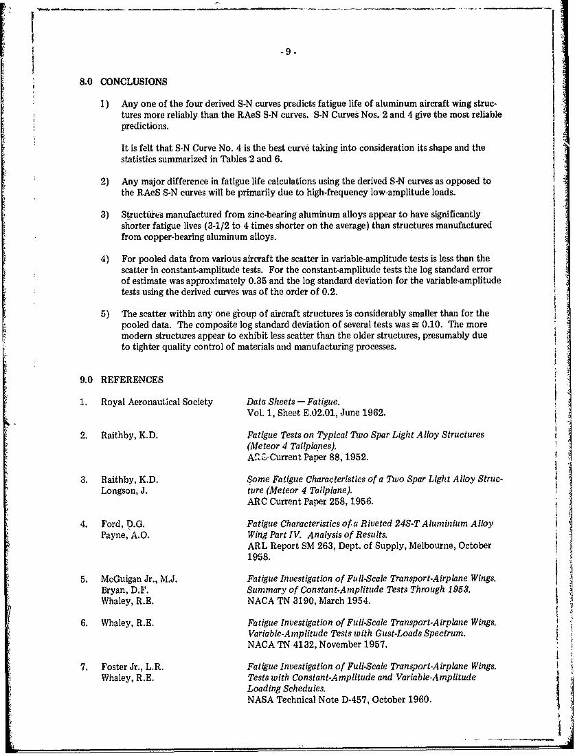
8.0 CONCLUSIONS
1) Any one of the four derived S-N curves predicts fatigue life of aluminum aircraft wing struc-tures more reliably than the RAeS S-N curves. S-N Curves Nos.-2 and 4 give the most reliablepredictions.
It is felt that S-N Curve No. 4 is the best curve taking into consideration its shape and thestatistics summarized in Tables2 and 6.
2) Any major difference in fatigue life calculations using the derived S-N curves as opposed tothe RAeS S-N curves will be primarily due to high-frequency low-amplitude loads.
3) Structures manufactured from zinc-bearing aluminum alloys appear to have significantlyshorter fatigue lives (3-1/2 to 4 times shorter on the average) than structures manufacturedfrom copper-bearing aluminum alloys.
4) For pooled data from various aircraft the scatter in variable-amplitude tests is less than thescatter in constant-amplitude tests. For the constant-amplitude tests the log standard errorof estimate was approximately 0.35 and the log standard deviation for the variable-amplitudetests using the derived curves was of the order of 0.2.
5) The scatter within any one group of aircraft structures is considerably smaller than for thepooled data. The composite log standard deviation of several tests was : 0.10. The moremodern structures appear to exhibit less scatter than the older structures, presumably dueto tighter quality control of materials and manufacturing processes.
9.0 REFERENCES
1. Royal Aeronautical Society Data Sheets - Fatigue.
Vol. 1, Sheet E.02.01, June 1962.
2. Raithby, K.D. Fatigue Tests on Typical Two Spar Light Alloy Structures(Meteor 4 Tailplanes).A &Current Paper 88, 1952.
3. Raithby, K.D. Some Fatigue Characteristics of a Two Spar Light Alloy Struc-Longson, J. ture (Meteor 4 Tailplane).
ARC Current Paper 258, 1956.
4. Ford, D.G. Fatigue Characteristics of a Riveted 24S-T Aluminium AlloyPayne, A.O. Wing Part IV. Analysis of Results.
ARL Report SM 263, Dept. of Supply, Melbourne, October1958.
5. McGuigan Jr., M.J. Fatigue Investigation of Full-Scale Transport-Airplane Wings.Bryan, D.F. Summary of Constant-Amplitude Tests Through 1953.Whaley, R.E. NACA TN 3190, March 1954.
6. Whaley, R.E. Fatigue Investigation of Full-Scale Transport-Airplane Wings.Variable-Amplitude Tests with Gust-Loads Spectrum.NACA TN 4132, November 1957.
7. Foster Jr., L.R. Fatigue Investigation of Full-Scale Transport-Airplane Wings.Whaley, R.E. Tests with Constant-Amplitude and Variable-Amplitude
Loading Schedules.NASA Technical Note D-457, October 1960.

-10-
8. Winkworth, W.J. P atigue Behaviour Under Service and Ground Test Conditions(A Comparison Based on the Dakota Wing).ARC Current Paper 666, 1964.
9. Raithby, K.D. Fatigue Testing of a Large Wing by the Resonance Method.RAE Report No. Structures 150, Farnborough, August 1953.
10. Carl, R.A. Investigations Concerning the Fatigue of Aircraft Structures.Wegend, T.J. ASTM Proceedings, Vol. 54, 1954, p. 903.
11. Rosenfeld, M.S. Aircraft Structural Fatigue Research in the Navy.
ASTM STP 338, Symposium on Fatigue of Aircraft Structures,
1962, p.216.
12. Swartz, R.P. Constant Amplitude Fatigue Characteristics of a Slab Hori-Rosenfeld, M.S. zontal Tail for a Typical Fighter Airplane.
U.S. Naval Air Material Center, Report-No. NAMATCEN-ASL-1023, Part 1, January 1960.
13. Zoudlik, R.J. Constant Amplitude Fatigue Characteristics of a Vertical TailRosenfeld, M.S. for a Typical Fighter Airplane.
U.S. Naval Air Material Center, Report No. ASL-1049, Part I,March 1962.
14. Ditchfield, C. Fatigue Life of the C-100 Mk 4 and Mk 5 Aircraft.Avro Aircraft Ltd., C-100/A/404, Issue C, December 1959.
15. Schijve, J. Fatigue Test Results of Three Full-Sca!e Wing Center 3ectionsde Rijk, P. Under Constant-Amplitude Loading.
NLR-TM S.640, Amsterdam, November 1965.
16. Hangartner, R. S-N Curves for Fatigue Life Prcdiction of Aluinbqum Ai-2raftWing Structures.Master's Thesis, University of Waterloo, Waterloo, Ontario,August 1974.
17. Sewell, R. T. An Investigation of Flight Loads, Counting Methods, andEffects on Estimated Fatigue Life.SAE Paper 720305, March 1972.
18. Douglas, R.B. An Investigation of Methods of Interpolating Between S-NCurves for the Endurance of Complete Wings and Tailplanesat Different Mean Stresses.Department of Civil Aviation, Aeronautical EngineeringReport SM-64, Australia, August 1972.
19. Parish, H.E. Fatigue Test Results and Analysis of 42 Piston Provost Wings.ARC R & M No. 3474, April 1965.
20. Payne, A.O. Random and Programmed Load Sequence Fatigue Tests on24S-T Aluminium Alloy Wings.ARL Report SM 244, Dept. of Supply, Melbourne, September1956.
21. Jost, G.S. A Comparison of Experimental and Predicted Fatigue LivesLewis, J.Y. of Mustang Wings Under Programmed and Random Loading.
ARL Report SM 300, Dept. of Supply, Melbourne, December1964.

-11 -
22. Patching, C.A. Comparison of a 2L.65 Aluminium Alloy Structure withMann, J.Y. Notched Specimens Under Programmed and Random Fatigue
Loading Sequences.Fatigue Design Procedures, Proceedings of the 4th ICAFSymposium, Edited by Gassner and Schitz, Munich 1965.
23. Dunsby, J.A. Fatigue Life Prediction of the CF-100 Aircraft.Pinkney, H.F.L. NRC, Aeronautical Report LR-438, National ResearchSewell, R.T. Council of Canada, Ottawa, Ontario, August 1965.Barszczewski, A.
24. Swartz, R.P. Variable Amplitude Fatigue Characteristics of a Slab Hori-Rosenfeld, M.S. zontal Tail for a Typical Fighter Airplne.
U.S. Naval Air Material Center Report No. NAMATCEN-ASL-1023, Part II, September 1961.
25. Schijve, J. Fatigue Tests With Random and Programmed Load SequencesBroek, D. With and Without Ground-to-Air Cycles. A Comparativede Rijk, P. Study on Full-Scale Wing Center Sections.Nederveen, A. NLR-TR S.613, Amsterdam, December 1965.Sevenhuysen, P.J.
26. Impellizzeri, L.F. Development of a Scatter Factor Applicable to Aircraft FatigueLife.ASTM STP 404, Structural Fatigue in Aircraft, 1966, p. 136.
I72;1

Preceding page blank -13.
TABLE 1
CONSTANT-AMPLITUDE DATA USED IN ANALYSIS
Aircraft Type and Component No. of Tests Reference
Meteor 4 Tailplane 36 2 and 3
P51D Mustang Wing 124 4
C-46 Commando Wing 18 5, 6, and 7
Dakota Wing 2 8
Lancaster Wing 1 9
Piston Aircraft* Outer Wing Panels 5 10
Piston Fighter* Wings 2 10
Jet Aircraft* Outer Wing Panels 7 10
F3H-1 Horizontal Tails 19 11 and 12
F3H-1 Vertical Tails 20 11 and 13
CF-100 Wings 9 14
Fokker F27 Wing Centre Section 3 15
Total Tests 246
* Aircraft type not disclosed in reference.

co w rLz to0w (0
0 0 c o- -
C C4 Cli C0 0a 00) 0
it coc1 cc)
0Bz LO c0 t- 0oto IT 6o v
o o co m
UL U)CiCD c ) cl co el
LI) v) 00 mCID vE- 0 e1 6 6
00
cnx
cc co
0 0
ci cn 00cc0
w) :. C)
0 C.)
00 0 0 to
0' cc 0) 0
0') ~C)0
+ t- I- + cl cc
-4 mt -4
0 0
c0 00 r- tr-
o~ ~ 0 cc00) ~6 JC) - 00
z 2: z: 2>) >) >)
u. C. C. u.
M:2 rn En

-15-
TABLE 3
VARIABLE-AMPLITUDE TESTS
Aircraft Reference
Piston Provost 19
P51D Mustang 20 and 21
Vampire 22
0-46 Commando 6 and 7
U.S. Navy Jet Fighter 10
CF-100 23
F3H-1 11 and 24
Fokker F27 25

CD toZ co LO D O ~ c 0 0
Sclc 1- 4: OCe l Ci) IR Ci' 0 1
N cl m q
6~ ~ oi C' \ C ,4 C6~ ID,
0 - c 00 w to -4
cn co cc,
0o N t- .-4 cc w' CD t-6t cc o- mD co 0- .- 0 t- toCl Cli cci ui4 - l --z
co 00a), CD Ci cc -: a; ci t- ctz c- -4 N~ 0 o -z IT -I
Nc IZ w C1l 00 wD vc m~ N
Qi Ci C) c cciDC3 Col r4 ee) c t- t -4
0, rn coc
b4 CI O 14 0 0 1- 0 1 - 0
7-d ;] I - cl Cc C; ci 14 cli
zz00 -T CID Cl
Oi ell co tD u-4 -4 0 4 t
CZ t-: qc cc: tC t C'I -ri- IEc ccr CID m c c Cl)
oo 0 o 0 l C6 4 (0 '-I Ir 0 Cl
-n 6I CD 6 0 0 m 0 CD L 6)
.2 - N 0)
C C
0CI

1-4 -IT 00 mo a) -T 0 C'1
C') U) Ci CR 0) C' Co C')CID c~ . C4 C13 14 m'
C) U
t- t - z 1-4 C11 uk l
Z. U -3 to
cl to 0- 0" "1 0R qD 0)o C co 6 cli co C13 vS c')
C)L to ) -
z C11 c')
C1)
to 0 LO 0 v-S c'
6~0~ C) C6 4- C') Cvi c' C')
C)1
C)Y ND ? ' --f 6r o o6 6' C' 6 U
u. -1 C1 v-00~ -
I- C') 1- t - ci t
Co co "T~ r'4 LD m- 16 O O CD
o 0C c -4 a' 00 0'i vs co
cn C11
oO co Q0 c') Co tUl) ci ( 5)ci m C) 0 0
w I
C)C) C) CO C; v- D ) U
0' C11 to CO to tv-v 00 v-S ) O C co
z, a-l c)c
L' i) NO ID c') H C) U)0
MO wCC C') V ) O to 0f to COW > C '4 C'- 6n v-4 v-v v- 04 v5)
0 --
C11 C))
it 6 0 06 ; 6 Z
-S0
C.,
U C') C') v-S C)(F 0n 0u cI (T. v-S 0 0

m cli co to E- L
Co?
'-4 0 0C t
000 0 0
IZ
M) m) 3 Co C11 T-1Nm N L 0 a)
O0C9 Co C* l- a C')~
0 H l 1 1
zz
oorX4 CO 0.
00 ~4 ~4 C6 6 4
E- C13 C o 11~3
N N Co 3) w 0)
0 q__ _ _
3) v 3) Co to CO
- - 0 0 0 0
> () z z z zZ0 W ) a
cO > > >
S Ch Ch CO CO

19 I-
00
0 ' 0a)
0 0
E 0 0
0- 0
oo
00 014 0
-~ -I- I- - -
N-
fc)
- - - -. to j0 < H
_L Li.
LO CL
(0
10
0 0 00 ___ 0_D_-_()_O'__)CN
10 ro) N~ - -
MS ")S MSJUB ONliVN831J2V

-20-
(0
cr C
C,
Zaa
ODD
zU,
C Nw wci, w
0-
- - -- (0 LL.1 w
L) w
0zw
7t/k I a
00 06 0 10 OO0f- (D1 r'o N -
!SM O SS38iS ESNlIVNd±1V

- 21 -
100 240C
LOG N-A+B LOG S LOG S = C+D LOG N10 1 0O 0I10 10COEFFICIENT A COEFFICIENT C
9"0 (INTERCEPT ON LOG N-AXIS) 2.00 (INTERCEPT ON LOG S.-AXIS),
8'0 2.200
7-0 2.100
0 5 10 15 20 25 30 0 5 10 15 20 25 30
MEAN STRESS KSI MEAN STRESS KSI
-5.0
COEFFICIENT B -0-350 COEFFICIENT D(SLOPE) (SLOPE)
-4.5
-0-300
-4.0
- 0-250
-0.200
- 3.00 5 10 15 20 25 30 0 5 10 15 20 2,5 30MEAN STRESS KSI MEAN STRESS KSI
FIG. 3: COEFFICIENTS OF EQUATIONS REPRESENTING
RAeS S-N CURVES VS MEAN STRESS

-22-
00 t0
6N
0to 0 0 0f
0 fo
00
-~j z
1- W- *iCO <
IN w
x *
CID
LO
XN to
00 0 0 10 0) COr-w (D LO o N~
'~ S SS38LLS 9NI1VN3V1h1V

-23-
_ _ 0)
-0(
N e - - - to0-n
O-r
(0
0i)
C~C
c to
-O 0 I
(0_ _ _ _ _ C
z
xw
U-)
0
00 0 0 0 MO 0)- (DW t4- ro
!SX ')S SS38LLS 9N11VN831-1V

-24-
+- IE OD
0 (0
a)
0
0
I Y
o CD
0O
(0
Cl)
0 w
U, ( I I I
00 D
LO~~ o C!SM D SS3IS ENliVHCiI

-25-
It) 0
- OD
o 00 1
0) 00 >
.1.
z
o 0-a)
-r - 0
COLLa
If) 5
z f
a) D
co(D
IVX I LYH
C\1
00
0 0 0 0 LO 0 0) co fl- w NoI o I
IS CIS SS38iS 9NUIVN831-1V

- 26 -
+ a) ______
0it) 0 QT
N -
w D a )w , (V
- -- 6 ___
Z0
* a)
zz0)0
o(l 0 D
CO< 0
_ _ ___
Coj
C~
0~~ zo~ ~ IC
0
0 i 0 ' )O- (0t t f l
to ro o 0MDS S3HI E)NiVN8i-N

- 27 -
+~0
--- 0 U - -- 4.o_0 (D- > -I _
CD 0
CDO~C.
ND P
C' 0j
2 ~0D
-) - r
U) F
C z a:
0-
CD J
- - 0 0 __0__ 0 _ ( ) ~ t \
Lo~ CO) ~_s DSHMSENlV81I

-28-
't0P, C0 J 0-_ >
- 0
t- o 0
.. I +z z
2
to
4Y
I--
0
E_-
L)
to 0 t 0 toN cli6
D S S381 DNIVN81-z

-29-
+E
0 0N ci(0D
(D_ (00
0) 0
0 00 0n
0 0
00
z Vli
xL I
I--
v I LL
0 U)
00
E
U,)
0 000
I__ _ _t_
- 'j __ _ ___
_ m S_ SS8_ 9NUN83

-30-
ft
- -- LE
0 0
mo to 0
@66 /_ IDC
3 z
s///.j -
-~ - i -_ o--1_
V X-
- 0to
/,i -iD0/
PI S 3-
_ /
u ) 0 It 0 0NJ N, - -
IS~l 0S SS3 11S 9NIiLNI3J17V,.

-31-
+
0
-j V), w
0 0(fu- 0
N Na'
0 0
toCO 0
IT 60o
-J C.)
x,____ ___ ___ __ _ __ _ _ __D
< oL
0
L))
w
o c
CC
C-
to 0 O 0 z_ _i _ _ _ /
'S SS8iS ENliVN3i-i

- 32-
I I I I
L-J
41 ci
'1 cii<3
W
<3<
L
<3%33 0) <34D< 0t N tr t ~C~j 6 6L
s-ivnoISw

-33-
w0
SZ E 0O i OtCQ to
z >
ZI
IL >
Iw I
0, 0/ 00 "to /~r / /j
S /S8i // 4VU~-

-34-
7I
76 r----------r-
0 A A~
I A
FI-1:ACULVPRDCEIVSFRN UV I (AL ALOS

__w 0
CZ to
.2s _ _ 0 (>z~ 0
_j _j _
__~L w_ _ o45-0-1 < CDN
I - F-_Z
__4 LO0 0 0__ 0 L D a
(NJ m D' 0)a
3nIV al~SNVI 13V O N18 O i-19V0K4u

-36-V
0 - nz 0
( 0wzV
___ ___ 0=) (D
___CI z_ I_ _
wI(n.
-L U-
zz
0
(D oU'
Jfl1VAz 63LVL 1VJ i3VU N3 OAIIVO /

-37-
0I00
- - 6 0_ _
z (b ww0 0 (n
ww>0 0 cr
(D w
C/)
CIZ -0-W co
(n- 4k
-v-- 0
_ _ W
z LL
(00
L9 zN0
- ~ toIf 0 0 0 0 00 0 0 0 fO co Cl)- N ro) it LO (D fl- OD) 0) CD C) 0)
]fl'A 031V.LS NVHJ. 831V389 ON139 N~JO AinlgvO0d 0 /%
- 38 -Ii
0-o
_L _ o111 a >~
wz
zW c
cl/,
-i J Z
0
cIZC N
- ~ ~ ~ ~ ~ ~ O N 00 00I)~0
N~~~~~~ >~
f L ~ ) 0 )0
BflVA JIIS VI4i J19US~NJ2 O JJ12VO~d0/

- 39 -
M 2 : ASSUMED
MEAN LIFE OF M- MEAN OFSAFE LIFE A FLEET OF VARIOUS AIRCRAFTOF FLEET AIRCRAFT STRUCTURES
3 a r2 3 o 1r
DISTRIBUTION
DISTRIBUTION
NO.2
SCATTER FACTOR USINGMINER'S RULE ( . n/N : I)AND -3or ON BOTH
S-N CURVE DISTRIBUTIONS
RAeS 0.05 0.10 1.32 L20
NO.1 0.24 0.47 2.13 "4
NO.2 0.30 0.59 2.24 .3
NO.3 0.31 0.61 2.45 "3NO.4 0.31 0.61 2.30 3
FIG.21: COMPARISON OF 2-n- VALUES FOR VARIOUS S-N CURVESAT EQUAL RELIABILITIES
T5

Preceding page blank -41-
APPENDIX I
METHODS FOR INTERPOLATING BETWEEN THE RAeS S-N CURVES
In general the equation of the curves are given as
log 1 0 N A + B'log10 Sa
1. Sewell's Method (Ref. 17)
Sm < 20 A = 9.45982 - 0.237677*Sn + 0.0118776*S2 - 0.00025697*S3
3.96687 - 0.021367*S m - 0.0004786*S2 + 0.00000657"S
2. Douglas' Method (Ref. 18)
0 < < 2 A = 10.0556 - 0.51285*Sm
B = 4.8023- 0.44000*Sm
2 < Sm < 15 Sewell's cubic polynominal expressions
15 < Sil < 20 A =8.5278 - 0.055198*Sm
B -3.9947- 0.028920*Sm -
20 < Sim < 30 A=8.3050 - 0.0 4 4 055*Sm
B = 3.9237 - 0.025373*Sni
8a, S' in ksi

Preceding page blank -43
MM Co r. N 0 % (N.C %
r 00000000
E4 C ON LO - CO T- C
00 r- %0 M0OnLOt
CO r- M MA 0 ~0 0
Zo m o - % .r
XT-r- m N mN (N (Nm
U. --z o to r- 4 .
M C W %0 M C * 4
Z ~ ~ ~ ~ V a) r- 4~ 33L A
IO ONOa)~
H M m . LAW M
V) E- W 0000 00 00 U
-I-
E- U) Ln0U L
-~~ 14. 00 0 0
04 0)N ... 0
U) . z ) -) u)uL Lnr 0 u) u)
C C C C 4 rn m
U) 1 W Uc
3C M4 C4~ ENN -4~~- 0 0Q) .ae m '
0 , ~ V) E-1Oe-N(