Lindsey A. Jasper and Bryan WelchGlenn Research Center, Cleveland, Ohio

Verification of an Icosahedral Grid for Strategic Center for Networking, Communications, and Integration User Interface Spatial Capabilities

NASA/TM—2018-219993

December 2018

NASA STI Program . . . in Profile

Since its founding, NASA has been dedicated to the advancement of aeronautics and space science. The NASA Scientific and Technical Information (STI) Program plays a key part in helping NASA maintain this important role.

The NASA STI Program operates under the auspices of the Agency Chief Information Officer. It collects, organizes, provides for archiving, and disseminates NASA’s STI. The NASA STI Program provides access to the NASA Technical Report Server—Registered (NTRS Reg) and NASA Technical Report Server—Public (NTRS) thus providing one of the largest collections of aeronautical and space science STI in the world. Results are published in both non-NASA channels and by NASA in the NASA STI Report Series, which includes the following report types: • TECHNICAL PUBLICATION. Reports of

completed research or a major significant phase of research that present the results of NASA programs and include extensive data or theoretical analysis. Includes compilations of significant scientific and technical data and information deemed to be of continuing reference value. NASA counter-part of peer-reviewed formal professional papers, but has less stringent limitations on manuscript length and extent of graphic presentations.

• TECHNICAL MEMORANDUM. Scientific

and technical findings that are preliminary or of specialized interest, e.g., “quick-release” reports, working papers, and bibliographies that contain minimal annotation. Does not contain extensive analysis.

• CONTRACTOR REPORT. Scientific and technical findings by NASA-sponsored contractors and grantees.

• CONFERENCE PUBLICATION. Collected papers from scientific and technical conferences, symposia, seminars, or other meetings sponsored or co-sponsored by NASA.

• SPECIAL PUBLICATION. Scientific,

technical, or historical information from NASA programs, projects, and missions, often concerned with subjects having substantial public interest.

• TECHNICAL TRANSLATION. English-

language translations of foreign scientific and technical material pertinent to NASA’s mission.

For more information about the NASA STI program, see the following:

• Access the NASA STI program home page at http://www.sti.nasa.gov

• E-mail your question to help@sti.nasa.gov • Fax your question to the NASA STI

Information Desk at 757-864-6500

• Telephone the NASA STI Information Desk at 757-864-9658 • Write to:

NASA STI Program Mail Stop 148 NASA Langley Research Center Hampton, VA 23681-2199

Lindsey A. Jasper and Bryan WelchGlenn Research Center, Cleveland, Ohio

Verification of an Icosahedral Grid for Strategic Center for Networking, Communications, and Integration User Interface Spatial Capabilities

NASA/TM—2018-219993

December 2018

National Aeronautics andSpace Administration

Glenn Research Center Cleveland, Ohio 44135

Acknowledgments

Lindsey A. Jasper thanks Bryan Welch and Dennis Rohn for their support and guidance. Both authors wish to thank the Space Communications and Navigation (SCaN) Summer Internship Project (SIP) program managers Tim Gallagher and Lindsay Hill for their hard work overseeing the program as well as the other interns on the SCaN Strategic Center for Networking, Integration, and Communications (SCENIC) team.

Available from

Trade names and trademarks are used in this report for identification only. Their usage does not constitute an official endorsement, either expressed or implied, by the National Aeronautics and

Space Administration.

Level of Review: This material has been technically reviewed by technical management.

NASA STI ProgramMail Stop 148NASA Langley Research CenterHampton, VA 23681-2199

National Technical Information Service5285 Port Royal RoadSpringfield, VA 22161

703-605-6000

This report is available in electronic form at http://www.sti.nasa.gov/ and http://ntrs.nasa.gov/

NASA/TM—2018-219993 1

Verification of an Icosahedral Grid for Strategic Center for Networking, Communications, and Integration

User Interface Spatial Capabilities

Lindsey A. Jasper* and Bryan Welch

National Aeronautics and Space Administration Glenn Research Center Cleveland, Ohio 44135

Summary Spatial communication analysis tools are incredibly useful resources to have when planning a space

mission. Every single mission that leaves Earth needs a way to send its data back down and every mission’s requirements on how that will be accomplished is different. Being able to analyze how existing assets can provide services independent of a specific mission can be key in that process. Most current commercial software packages contain spatial analysis capabilities but go about the analysis in a way that is not the most efficient and can skew the results provided. NASA’s Space Communications and Navigation (SCaN) Strategic Center for Networking, Integration, and Communications (SCENIC) seeks to solve this problem and provide analysis capabilities by using both internally developed and open-source software. This allows incredible flexibility and customization and hugely reduces licensing costs. Using MATLAB® (MathWorks®) and Orbit Determination Toolbox created by Goddard Space Flight Center, SCENIC is able to perform many node-based functions currently. Analysis utilizing the spatial tools in SCENIC allows a meaningful analysis of the capability of communication network assets in a way not seen in current commercial software packages. This paper discusses the verification activities associated with generating the spatial grid point definition utilized in these analysis capabilities within the SCENIC user interface (UI).

Nomenclature

FOV field of view SCaN Space Communications and Navigation SCENIC Strategic Center for Networking, Integration, and Communications UI user interface

Symbols A area Ax,y,z x, y, or z coordinate of A vertex a segment length (across from vertex a) b segment length (across from vertex b) Bx,y,z x, y, or z coordinate of B vertex c segment length (across from vertex c) Cx,y,z x, y, or z coordinate of C vertex D distance Ox,y,z coordinate set of the centroid of a triangle s half perimeter of a triangle

*Pathways Intern at NASA Glenn Research Center

NASA/TM—2018-219993 2

1.0 Introduction The necessity for proper spatial analysis of communication systems is a pressing problem. When

designing a system or performing system analysis, it is not always known what existing assets can provide to a new mission or how they can be improved to better serve the network. This is where spatial analysis becomes an incredibly useful tool. Spatial analysis does not require the engineer to have full knowledge of what the new elements will look like prior to analysis, but allows them to analyze the capability of the system, visualizing and producing data for what the signal will be like when projected onto a volume of altitude around a body.

Various commercial software packages for space systems analysis currently have this capability, but there are several downsides to how spatial analysis is implemented in commercial software packages. In order to generate the spatial volume of analysis interest to perform the analysis over, most commercial software generates a grid of points around the body where each point is a vertex on a rectangle, laid out similarly to latitude and longitude over a body. Though this type of grid is by far the easiest to implement, it creates several problems. The first of these problems created by using a square grid is oversampling of data at the poles. Attempts are made to solve this issue by applying a weighting factor to the grid of points that is dependent on the cosine of the latitude. While this does solve some of the problems of the unevenly clustered points, it does not fully provide a solution, as the weighting causes the points and the north and south poles to be zero. The Space Communications and Navigation (SCaN) Strategic Center for Networking, Integration, and Communications (SCENIC) seeks to solve these existing problems by utilizing an icosahedral grid that is generated in MATLAB® (MathWorks®) with user-defined parameters and then feeding that grid into the spatial analysis tools (Figure 1). This not only cuts down on software costs, as commercial packages can be costly, but also enables high flexibility and customization of current and future capabilities.

The spatial capabilities of SCENIC affect nearly all areas of its communications analysis abilities. Besides communications, SCENIC performs orbit and trajectory propagation with tools that support both of those functions, as it is important to not only analyze the communications capabilities of these space systems but also to be able to know their current state. This knowledge provides better communications data and enables some capabilities such as line of sight, which gives the user the ability to know when a spacecraft is visible to their antenna and the window of time they have to communicate with it. In the future, all of these capabilities will be enabled on into the SCENIC user interface (UI).

Figure 1.—Spatial analysis tool grids. (a) Most commonly

used grid in spatial analysis tools where convergence of points at poles is easily visible. (b) Strategic Center for Networking, Integration, and Communications’ proposed solution with no visible convergence of points at any location on sphere.

NASA/TM—2018-219993 3

2.0 Methodology The process to create the grid of points over which to do the analysis was driven by the desire to

create the aforementioned grid easily, quickly, and in a way that resulted in the most evenly spaced grid of points as possible. This led to the utilization of an existing function, icosphere (Refs. 1 and 2). While another function was originally considered, the initial function was found to have some slight inconsistencies in the location of the points, which is described later in this paper. While the source of these inconsistencies is unknown, it may be due to reliance on a separate subdivision function, which may not have been the most accurate. This drove the search to find a different function. This function relies on an existing MATLAB® (MathWorks®) definition of an icosahedron and projects the vertices onto a unit sphere (Figure 2), outputting the new coordinates of the vertices. Depending on the desired resolution of the grid, it subdivides each triangular face into four new faces by bisecting each side of the initial equilateral triangle (Figure 3).

The output of this initial function contained the vertices of each triangular face. Though this is a feasible way of creating the grid, it was decided to perform the analysis over a grid of points made up of the centroids of each face for user friendliness. This was accomplished by sorting the vertices into faces and then looping over each face with the centroid formula (Eq. (1)) to yield the centroid of each face in Cartesian coordinates and sorting them into separate x, y, and z matrices before concatenating them into a larger matrix containing the Cartesian coordinates for each centroid.

, , , , , ,, , 3

x y z x y z x y zx y z

A B CO

+ += (1)

Figure 2.—Example of icosahedron full subdivision up to second subdivision.

Figure 3.—Example of icosahedron face division up to second subdivision.

NASA/TM—2018-219993 4

From there, the points were then converted into latitude and longitude (while being kept a unit radius) so the user could more easily specify a set of latitude and longitude coordinates to constrain the analysis. A script was then created to verify that the points generated by the function were that of an icosahedron. The function was verified by calculating the area of each face and comparing it to the areas of the other faces. This was accomplished by sorting each face into A, B, and C vertices and then calculating the distance from A to B, B to C, and A to C by using the distance formula (Eq. (2)) looping over all faces.

( ) ( ) ( )2 2 2A B A B A BD x x y y z z= − + − + − (2)

Finally, the area for each face was calculated by using Heron’s formula (Ref. 3) (Eqs. (3) and (4)).

2a b cs + +

= (3)

( )( )( )A s s a s b s c= − − − (4)

Here, Heron’s formula is used because of the ease it offers when calculating the area of each triangle given the side lengths, which were previously calculated. Since each triangle is not a right triangle but an isosceles, it is logical to use side lengths, which were already calculated, instead of using the base length and the height, which cannot be found with a single computation.

In the initial icosahedron, it can be assumed that the triangles are equilateral, as the definition of a regular icosahedron describes. Each vertex is equidistant from the five other vertices, so the assumption can be made that all 20 faces would have the same area. After the first subdivision, that assumption can no longer be made. The icosahedron created is no longer regular, because during the first subdivision, some vertices still touch the initial five other vertices but some (the new vertices) touch six other vertices (Figure 4).

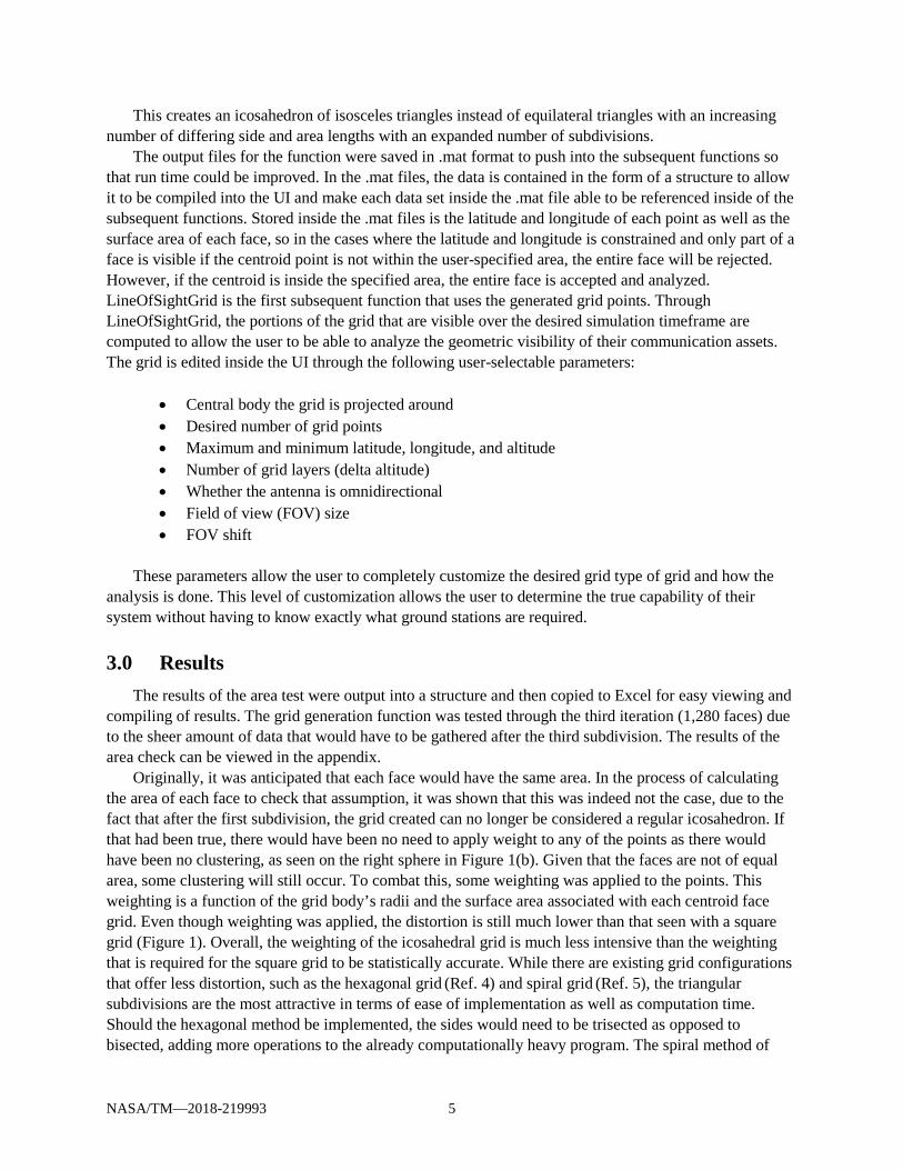
This creates an icosahedron of isosceles triangles instead of equilateral triangles with an increasing number of differing side and area lengths with an expanded number of subdivisions.

Figure 4.—Irregular icosahedron with

some vertices neighboring five other vertices (red highlighted) and some neighboring six (green highlighted).

NASA/TM—2018-219993 5

This creates an icosahedron of isosceles triangles instead of equilateral triangles with an increasing number of differing side and area lengths with an expanded number of subdivisions.

The output files for the function were saved in .mat format to push into the subsequent functions so that run time could be improved. In the .mat files, the data is contained in the form of a structure to allow it to be compiled into the UI and make each data set inside the .mat file able to be referenced inside of the subsequent functions. Stored inside the .mat files is the latitude and longitude of each point as well as the surface area of each face, so in the cases where the latitude and longitude is constrained and only part of a face is visible if the centroid point is not within the user-specified area, the entire face will be rejected. However, if the centroid is inside the specified area, the entire face is accepted and analyzed. LineOfSightGrid is the first subsequent function that uses the generated grid points. Through LineOfSightGrid, the portions of the grid that are visible over the desired simulation timeframe are computed to allow the user to be able to analyze the geometric visibility of their communication assets. The grid is edited inside the UI through the following user-selectable parameters:

• Central body the grid is projected around • Desired number of grid points • Maximum and minimum latitude, longitude, and altitude • Number of grid layers (delta altitude) • Whether the antenna is omnidirectional • Field of view (FOV) size • FOV shift

These parameters allow the user to completely customize the desired grid type of grid and how the

analysis is done. This level of customization allows the user to determine the true capability of their system without having to know exactly what ground stations are required.

3.0 Results The results of the area test were output into a structure and then copied to Excel for easy viewing and

compiling of results. The grid generation function was tested through the third iteration (1,280 faces) due to the sheer amount of data that would have to be gathered after the third subdivision. The results of the area check can be viewed in the appendix.

Originally, it was anticipated that each face would have the same area. In the process of calculating the area of each face to check that assumption, it was shown that this was indeed not the case, due to the fact that after the first subdivision, the grid created can no longer be considered a regular icosahedron. If that had been true, there would have been no need to apply weight to any of the points as there would have been no clustering, as seen on the right sphere in Figure 1(b). Given that the faces are not of equal area, some clustering will still occur. To combat this, some weighting was applied to the points. This weighting is a function of the grid body’s radii and the surface area associated with each centroid face grid. Even though weighting was applied, the distortion is still much lower than that seen with a square grid (Figure 1). Overall, the weighting of the icosahedral grid is much less intensive than the weighting that is required for the square grid to be statistically accurate. While there are existing grid configurations that offer less distortion, such as the hexagonal grid (Ref. 4) and spiral grid (Ref. 5), the triangular subdivisions are the most attractive in terms of ease of implementation as well as computation time. Should the hexagonal method be implemented, the sides would need to be trisected as opposed to bisected, adding more operations to the already computationally heavy program. The spiral method of

NASA/TM—2018-219993 6

generation, while attractive, has not been researched enough to be considered a viable method at the time of publication. Even though they may not provide the most accurate analysis of each of the current methods, the triangular subdivisions also offer an advantage in that the weighting of the points allows the icosahedral grid to be better than the spatial analysis capabilities most commercial software packages include.

It was also anticipated that with an increasing number of subdivisions, the icosahedron’s total surface area would converge to the total surface area of the sphere it was approximating. This was reflected well in the data and was tested for two different cases: a unit sphere and a sphere of radius 2.

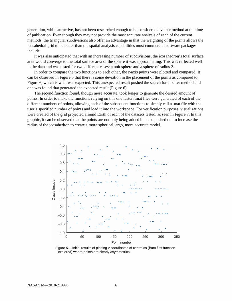
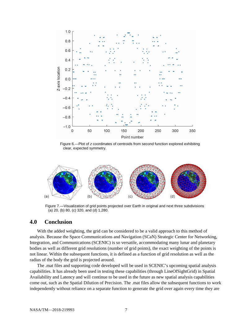
In order to compare the two functions to each other, the z-axis points were plotted and compared. It can be observed in Figure 5 that there is some deviation in the placement of the points as compared to Figure 6, which is what was expected. This unexpected result pushed the search for a better method and one was found that generated the expected result (Figure 6).

The second function found, though more accurate, took longer to generate the desired amount of points. In order to make the functions relying on this one faster, .mat files were generated of each of the different numbers of points, allowing each of the subsequent functions to simply call a .mat file with the user’s specified number of points and load it into the workspace. For verification purposes, visualizations were created of the grid projected around Earth of each of the datasets tested, as seen in Figure 7. In this graphic, it can be observed that the points are not only being added but also pushed out to increase the radius of the icosahedron to create a more spherical, ergo, more accurate model.

Figure 5.—Initial results of plotting z coordinates of centroids (from first function

explored) where points are clearly asymmetrical.

NASA/TM—2018-219993 7

Figure 6.—Plot of z coordinates of centroids from second function explored exhibiting

clear, expected symmetry.

Figure 7.—Visualization of grid points projected over Earth in original and next three subdivisions

(a) 20, (b) 80, (c) 320, and (d) 1,280.

4.0 Conclusion With the added weighting, the grid can be considered to be a valid approach to this method of

analysis. Because the Space Communications and Navigation (SCaN) Strategic Center for Networking, Integration, and Communications (SCENIC) is so versatile, accommodating many lunar and planetary bodies as well as different grid resolutions (number of grid points), the exact weighting of the points is not linear. Within the subsequent functions, it is defined as a function of grid resolution as well as the radius of the body the grid is projected around.

The .mat files and supporting code developed will be used in SCENIC’s upcoming spatial analysis capabilities. It has already been used in testing these capabilities (through LineOfSightGrid) in Spatial Availability and Latency and will continue to be used in the future as new spatial analysis capabilities come out, such as the Spatial Dilution of Precision. The .mat files allow the subsequent functions to work independently without reliance on a separate function to generate the grid over again every time they are

NASA/TM—2018-219993 8

run, and they also allow updates to the type of grid to take place without too many major changes to the subsequent functions.

There are a few opportunities for future work with this grid, one of the main ones being expanding the amount of options available (not only the triangular-faced icosahedral form). The other types of grid options available, such as the hexagonal or spiral grid (though requiring more backend work), might allow for an even more meaningful analysis.

NASA/TM—2018-219993 9

Appendix A.1 Icosahedron Approximating Sphere of Radius 1

Figure 8 to Figure 11 show the face number and corresponding surface area for various icosahedron face counts and Table I to Table IV list the surface areas for the corresponding face counts.

Figure 8.—Face number and the corresponding surface area for a 20-face icosahedron

approximating a unit sphere.

Figure 9.—Face number and the corresponding surface area for an 80-face icosahedron

approximating a unit sphere.

NASA/TM—2018-219993 10

Figure 10.—Face number and the corresponding surface area for a 320-face

icosahedron approximating a unit sphere.

Figure 11.—Face number and the corresponding surface area for a 1,280-face icosahedron

approximating a unit sphere.

TABLE I.—TOTAL SURFACE AREA OF THE 20-FACE ICOSAHEDRON

APPROXIMATING A UNIT SPHERE Surface area

Icosahedron ...................................... 9.575

Sphere .............................................. 12.57

NASA/TM—2018-219993 11

TABLE II.—TOTAL SURFACE AREA OF THE 80-FACE ICOSAHEDRON

APPROXIMATING A UNIT SPHERE Surface area

Icosahedron .....................................11.666

Sphere .............................................. 12.57

TABLE III.—TOTAL SURFACE AREA OF THE 320-FACE ICOSAHEDRON APPROXIMATING A UNIT SPHERE

Surface area

Icosahedron ...................................... 12.33

Sphere .............................................. 12.57

TABLE IV.—TOTAL SURFACE ARE OF THE 1,280-FACE ICOSAHEDRON APPROXIMATING A UNIT SPHERE

Surface area

Icosahedron .....................................12.506

Sphere .............................................. 12.57

Figure 12.—Face number and the corresponding surface area for a 20-face

icosahedron approximating a sphere of radius 2.

A.2 Icosahedron Approximating Sphere of Radius 2

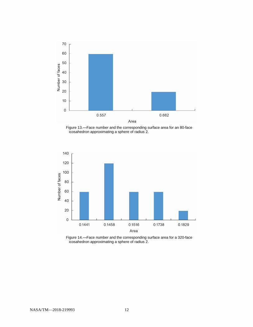
Figure 12 to Figure 15 show the face number and corresponding surface area for various icosahedron face counts and Table V to Table VIII list the surface areas for the corresponding face counts.

NASA/TM—2018-219993 12

Figure 13.—Face number and the corresponding surface area for an 80-face

icosahedron approximating a sphere of radius 2.

Figure 14.—Face number and the corresponding surface area for a 320-face

icosahedron approximating a sphere of radius 2.

NASA/TM—2018-219993 13

Figure 15.—Face number and the corresponding surface area for a 1,280-face

icosahedron approximating a sphere of radius 2.

TABLE V.—TOTAL SURFACE AREA OF THE 20-FACE ICOSAHEDRON

APPROXIMATING A SPHERE OF RADIUS 2 Surface area

Icosahedron .....................................38.928

Sphere .............................................. 50.27

TABLE VI.—TOTAL SURFACE AREA OF THE 80-FACE ICOSAHEDRON

APPROXIMATING A SPHERE OF RADIUS 2 Surface area

Icosahedron .....................................46.664

Sphere .............................................. 50.27

TABLE VII.—TOTAL SURFACE AREA OF THE 320-FACE ICOSAHEDRON

APPROXIMATING A SPHERE OF RADIUS 2 Surface area

Icosahedron .....................................49.319

Sphere .............................................. 50.27

TABLE VIII.—TOTAL SURFACE AREA OF THE 1,280-FACE ICOSAHEDRON

APPROXIMATING A SPHERE OF RADIUS 2 Surface area

Icosahedron .....................................50.026

Sphere .............................................. 50.27

NASA/TM—2018-219993 14

References 1. Kahler, Andreas: Creating an Icosphere Mesh in Code. 2009.

http://blog.andreaskahler.com/2009/06/creating-icosphere-mesh-in-code.html Accessed Nov. 21, 2018.

2. Sahr, Kevin; White, Denis; and Kimerling, A. Jon: Geodesic Discrete Global Grid Systems. Cartogr. Geogr. Inf. Sci., vol. 30, no. 2, 2003, pp. 121–134.

3. Salamonczyk, Andrzej; and Mokrzycki, Wojciech: Generation of View Representation From View Points of Spiral Trajectory. Ryszard S. Choras, ed., Image Processing and Communications Challenges 2, Vol. 84. Springer-Verlag Berlin Heidelberg, 2010, pp. 67–74.

4. Ward, Wil O.C.: icosphere.m. March 19, 2015. http://www.mathworks.com/matlabcentral/mlc-downloads/downloads/submissions/50105/versions/3/previews//icosphere.m/index.html?access_key= Accessed Nov. 21, 2018.

5. Weisstein, Eric W.: Heron's Formula. MathWorld, Wolfram Research, Inc., 2018. http://mathworld.wolfram.com/HeronsFormula.html Accessed Nov. 21, 2018.