9. Orbits in stationary Potentials

We have seen how to calculate forces and

potentials from the smoothed density ρ.

Now we can analyse how stars move in this

potential. Because two body interactions

can be ignored, we can analyse each star by

itself. We therefore speak of “orbits”. The

main aim is to focus on the properties of

orbits. Given a potential, what orbits are

possible?

Overview

9.1 Orbits in spherical potentials

(BT p. 103-107)

9.2 Constants and Integrals of motion

(BT p. 110-117)

9.2.1 Spherical potentials

9.2.2 Integrals in 2 dimensional flattened

potentials

9.2.3 Axisymmetric potentials

9.3 A general 3-dimensional potential

9.4 Schwarzschild’s method 1

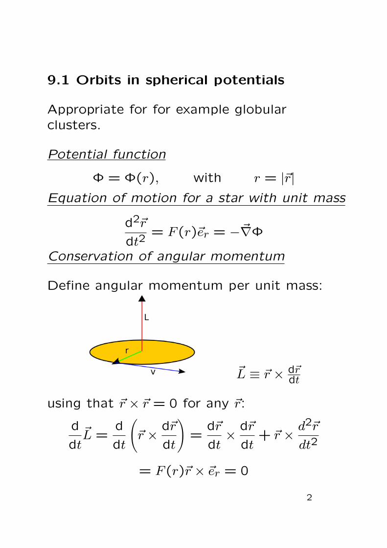
9.1 Orbits in spherical potentials

Appropriate for for example globularclusters.

Potential function

Φ = Φ(r), with r = |~r|Equation of motion for a star with unit mass

d2~r

dt2= F (r)~er = −~∇Φ

Conservation of angular momentum

Define angular momentum per unit mass:

~L ≡ ~r × d~rdt

using that ~r × ~r = 0 for any ~r:

d

dt~L =

d

dt

(~r ×

d~r

dt

)=

d~r

dt×

d~r

dt+ ~r ×

d2~r

dt2

= F (r)~r × ~er = 0

2

Hence ~L = ~r × ~r is constant with time. ~L isalways perpendicular to the plane in which ~r

and ~v lie. Since it is constant with time,these vectors always lie in the same plane.Hence the orbit is constrained to this orbitalplane. Geometrically, L is equal to twice therate at which the radius vector sweeps outarea.

Use polar coordinates (r, ψ) in orbital planeand rewrite equations of motion in polarcoordinates

Using BT (App. B.2), the acceleration d2~rdt2

in cylindrical coordinates can be written as:

d2~r

dt2= (r − rψ2)~er + (2rψ + rψ)~eψ

With the equation of motion d2~rdt2

= F (r)~er,this implies:

r − rψ2 = F (r) (∗)

2rψ + rψ = 0 (∗∗)

3

Hence:

2rψ + rψ =1

r

dr2ψ

dt= 0 ⇒ r2ψ = rv⊥ = L = cst

Using ψ = Lr2 and equation (**):

r − rψ2 = r −L2

r3= −

dΦ

dr3 where Φ is the potential.

Integrate last equation to obtain:

12r

2 = E −Φ−L2

2r2= E −Φeff(r)

with E the energy. E is the integrationconstant obtained for r →∞

This equation governs radial motionthrough the effective potential Φeff:

Φeff = Φ +L2

2r2

4

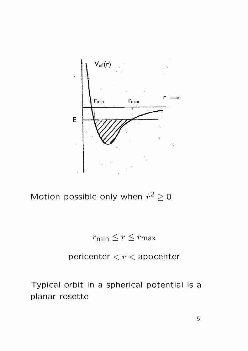
rmaxrmin

Veff(r)

r

E

Motion possible only when r2 ≥ 0

rmin ≤ r ≤ rmax

pericenter < r < apocenter

Typical orbit in a spherical potential is a

planar rosette

5

Angle ∆ψ between successive apocenter

passages depends on mass distribution:

π (homogeneous sphere) < ∆ψ < 2π (pointmass)

6

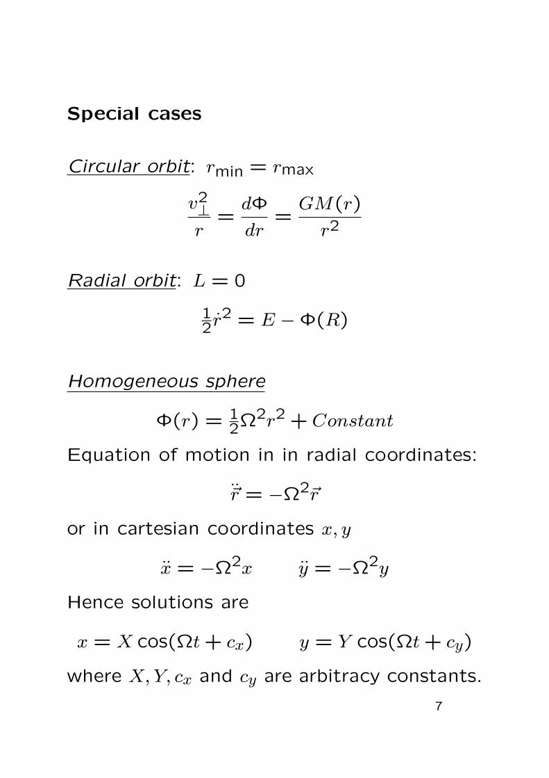
Special cases

Circular orbit: rmin = rmax

v2⊥r

=dΦ

dr=GM(r)

r2

Radial orbit: L = 0

12r

2 = E −Φ(R)

Homogeneous sphere

Φ(r) = 12Ω2r2 + Constant

Equation of motion in in radial coordinates:

~r = −Ω2~r

or in cartesian coordinates x, y

x = −Ω2x y = −Ω2y

Hence solutions are

x = X cos(Ωt+ cx) y = Y cos(Ωt+ cy)

where X,Y, cx and cy are arbitracy constants.

7

Hence, even though energy and angular

momentum restrict orbit to a “rosetta”,

these orbits are even more special: they do

not fill the area between the minimum and

maximum radius, but are always closed !

The same holds for Kepler potential. But

beware, for the homogeneous sphere the

particle does two radial excursions per cycle

around the center, for the Kepler potential,

it does one radial excursion per angular

cycle.

We now wish to “classify” orbits and their

density distribution in a systematic way. For

that we use integrals of motion.

8

9.2 Constants and Integrals of motion

First, we define the 6 dimensional “phase

space” coordinates (~x,~v). They are

conveniently used to describe the motions

of stars. Now we introduce:

• Constant of motion: a function

C(~x,~v, t) which is constant along any

orbit:

C(~x(t1), ~v(t1), t1) = C(~x(t2), ~v(t2), t2)

C is a function of ~x, ~v, and time t.

• Integral of motion: a function I(~x,~v)

which is constant along any orbit:

I[~x(t1), ~v(t1)] = I[~x(t2), ~v(t2)]

9

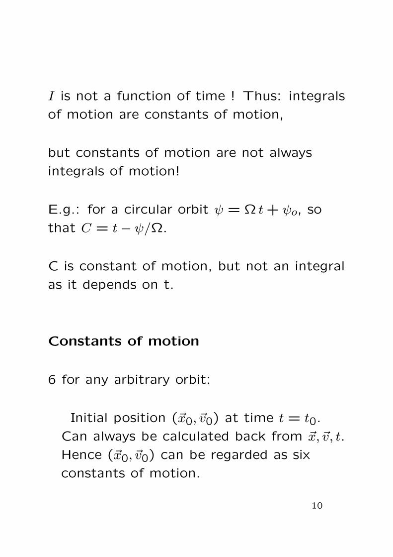
I is not a function of time ! Thus: integrals

of motion are constants of motion,

but constants of motion are not always

integrals of motion!

E.g.: for a circular orbit ψ = Ω t+ ψo, so

that C = t− ψ/Ω.

C is constant of motion, but not an integral

as it depends on t.

Constants of motion

6 for any arbitrary orbit:

Initial position (~x0, ~v0) at time t = t0.

Can always be calculated back from ~x,~v, t.

Hence (~x0, ~v0) can be regarded as six

constants of motion.

10

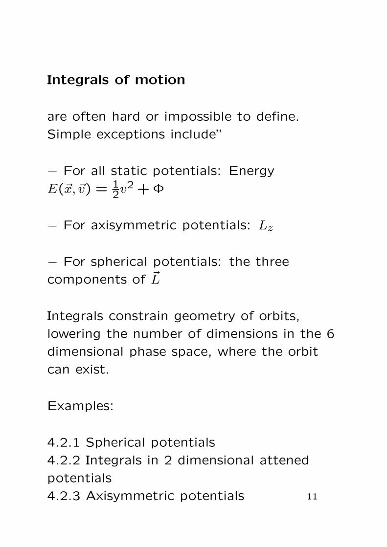
Integrals of motion

are often hard or impossible to define.

Simple exceptions include”

− For all static potentials: Energy

E(~x,~v) = 12v

2 + Φ

− For axisymmetric potentials: Lz

− For spherical potentials: the three

components of ~L

Integrals constrain geometry of orbits,

lowering the number of dimensions in the 6

dimensional phase space, where the orbit

can exist.

Examples:

4.2.1 Spherical potentials

4.2.2 Integrals in 2 dimensional attened

potentials

4.2.3 Axisymmetric potentials 11

9.2.1. Spherical potentials

E,Lx, Ly, Lz are integrals of motion, but alsoE, |L| and the direction of ~L (given by theunit vector ~n, which is defined by twoindependent numbers). ~n defines the planein which ~x and ~v must lie. Definecoordinate system with z axis along ~n

~x = (x1, x2,0)

~v = (v1, v2,0)

→ ~x and ~v constrained to 4D region of the6D phase space. In this 4 dimensionalspace, |L| and E are conserved. Thisconstrains the orbit to a 2 dimensionalspace. Hence the velocity is uniquelydefined for a given ~x (see page 4).

vr = ±√

2(E −Φ)− L2/r2

vψ = ±L/r

12

9.2.2. Integrals in 2 dimensional

flattened potentials

Examples:

• Circular potential V (x, y) = V (~r)

Two integrals: E,Lz.

• Flattened potential

V (x, y) = ln(x2 + y2

a + 1)

Only “classic” integral of motion: E

Figures on the next page show the orbits

that one gets by integrating the equations

of motion this flattened potential

13

Box orbits no net angular momentum,

(Lz = x ∗ vy − y ∗ vx)

avoid outer x-axis

-4 -2 0 2 4

-4

-2

0

2

4

x0=0.5 y0=0 vx0=0 vy0=1

-4 -2 0 2 4

-4

-2

0

2

4

x0=1 y0=0 vx0=0 vy0=1

-4 -2 0 2 4

-4

-2

0

2

4

x0=1.1 y0=0 vx0=0 vy0=1

-4 -2 0 2 4

-4

-2

0

2

4

x0=1.2 y0=0 vx0=0 vy0=1

-4 -2 0 2 4

-4

-2

0

2

4

x0=0.5 y0=0 vx0=0 vy0=1

-4 -2 0 2 4

-4

-2

0

2

4

x0=1 y0=0 vx0=0 vy0=1

-4 -2 0 2 4

-4

-2

0

2

4

x0=1.1 y0=0 vx0=0 vy0=1

-4 -2 0 2 4

-4

-2

0

2

4

x0=1.2 y0=0 vx0=0 vy0=1

-4 -2 0 2 4

-4

-2

0

2

4

x0=0.5 y0=0 vx0=0 vy0=1

-4 -2 0 2 4

-4

-2

0

2

4

x0=1 y0=0 vx0=0 vy0=1

-4 -2 0 2 4

-4

-2

0

2

4

x0=1.1 y0=0 vx0=0 vy0=1

-4 -2 0 2 4

-4

-2

0

2

4

x0=1.2 y0=0 vx0=0 vy0=1

14

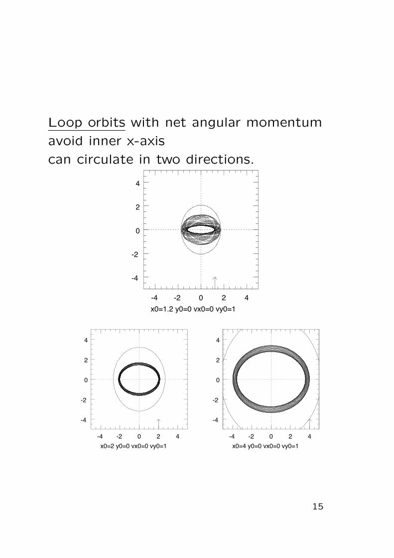
Loop orbits with net angular momentum

avoid inner x-axis

can circulate in two directions.-4 -2 0 2 4

-4

-2

0

2

4

x0=0.5 y0=0 vx0=0 vy0=1

-4 -2 0 2 4

-4

-2

0

2

4

x0=1 y0=0 vx0=0 vy0=1

-4 -2 0 2 4

-4

-2

0

2

4

x0=1.1 y0=0 vx0=0 vy0=1

-4 -2 0 2 4

-4

-2

0

2

4

x0=1.2 y0=0 vx0=0 vy0=1

-4 -2 0 2 4

-4

-2

0

2

4

x0=2 y0=0 vx0=0 vy0=1

-4 -2 0 2 4

-4

-2

0

2

4

x0=4 y0=0 vx0=0 vy0=1

15

Clearly the orbits are regular and do not fill

equipotential surface

Furthermore, they do not traverse each

point in a random direction, but generally

only in 2 directions

Conclusion: the orbits do not occupy a 3

dimensional space in the 4-dimensional

phase-space, but they occopy only a

2-dimensional space !

This indicates that there is an additional

integral of motion: ’a non-classical

integral’

The non-classical integral, plus the regular

’Energy’, constrain the orbit to lie on a 2

dimensional surface in the 4 dimensional

phase-space.

16

A homogeneous ellipsoid

The homogeneous ellipsoid helps us to

understand how additional integrals of

motions, and box orbits, exist. Consider a

density distribution:

ρ = ρ0H(1−m2),

with m2 = x2

a2 + y2

b2+ z2

c2

and H(x) = 1 for x ≥ 0, H(x) = 0 for

x < 0

Potential inside the ellipsoid:

Φ = Axx2 +Ayy

2 +Azz2 + C0

Forces are of the form Fi = −Aixi, i.e. 3

independent harmonic oscillators:

xi = ai cos(ωit+ ψ0,i)

3 integrals of motion, Ei17

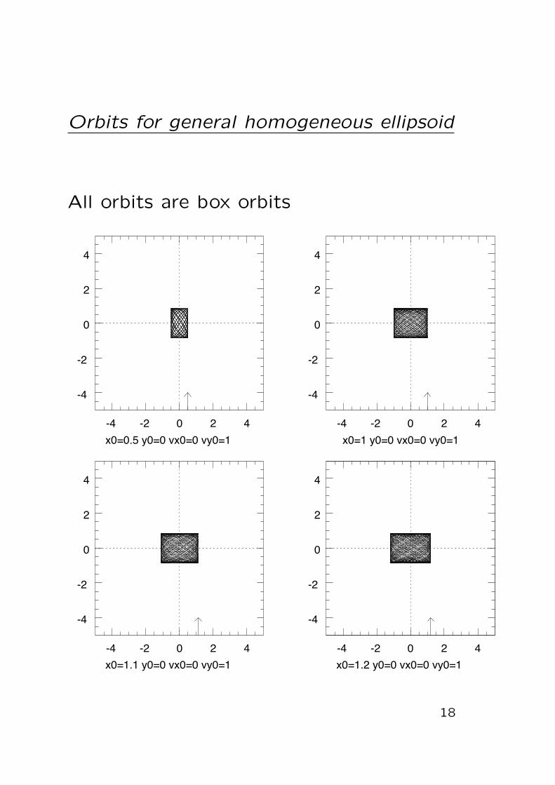
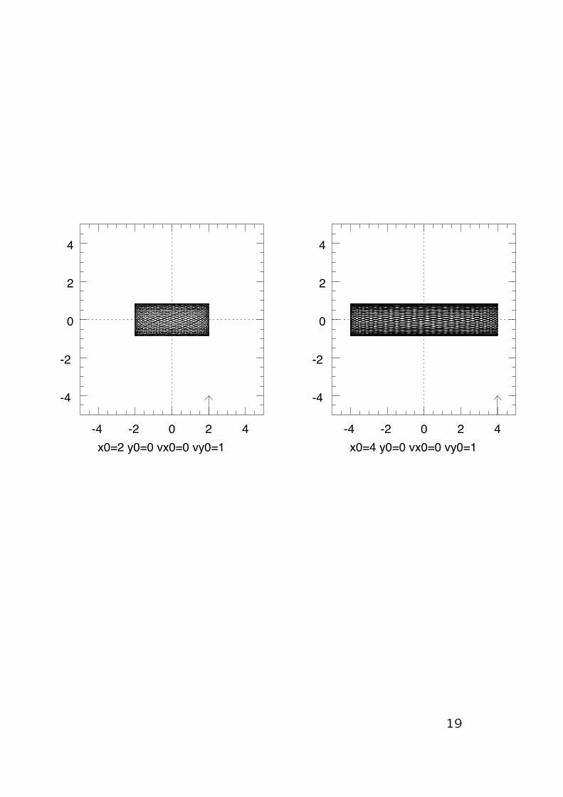
Orbits for general homogeneous ellipsoid

All orbits are box orbits

-4 -2 0 2 4

-4

-2

0

2

4

x0=0.5 y0=0 vx0=0 vy0=1 -4 -2 0 2 4

-4

-2

0

2

4

x0=1 y0=0 vx0=0 vy0=1

-4 -2 0 2 4

-4

-2

0

2

4

x0=1.1 y0=0 vx0=0 vy0=1 -4 -2 0 2 4

-4

-2

0

2

4

x0=1.2 y0=0 vx0=0 vy0=1

18

-4 -2 0 2 4

-4

-2

0

2

4

x0=2 y0=0 vx0=0 vy0=1 -4 -2 0 2 4

-4

-2

0

2

4

x0=4 y0=0 vx0=0 vy0=1

19

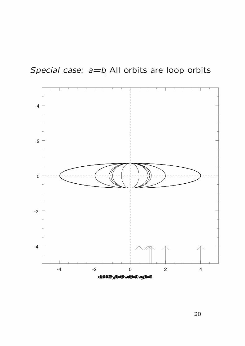
Special case: a=b All orbits are loop orbits

-4 -2 0 2 4

-4

-2

0

2

4

x0=0.5 y0=0 vx0=0 vy0=1 x0=1 y0=0 vx0=0 vy0=1 x0=1.1 y0=0 vx0=0 vy0=1 x0=1.2 y0=0 vx0=0 vy0=1 x0=2 y0=0 vx0=0 vy0=1 x0=4 y0=0 vx0=0 vy0=1

20

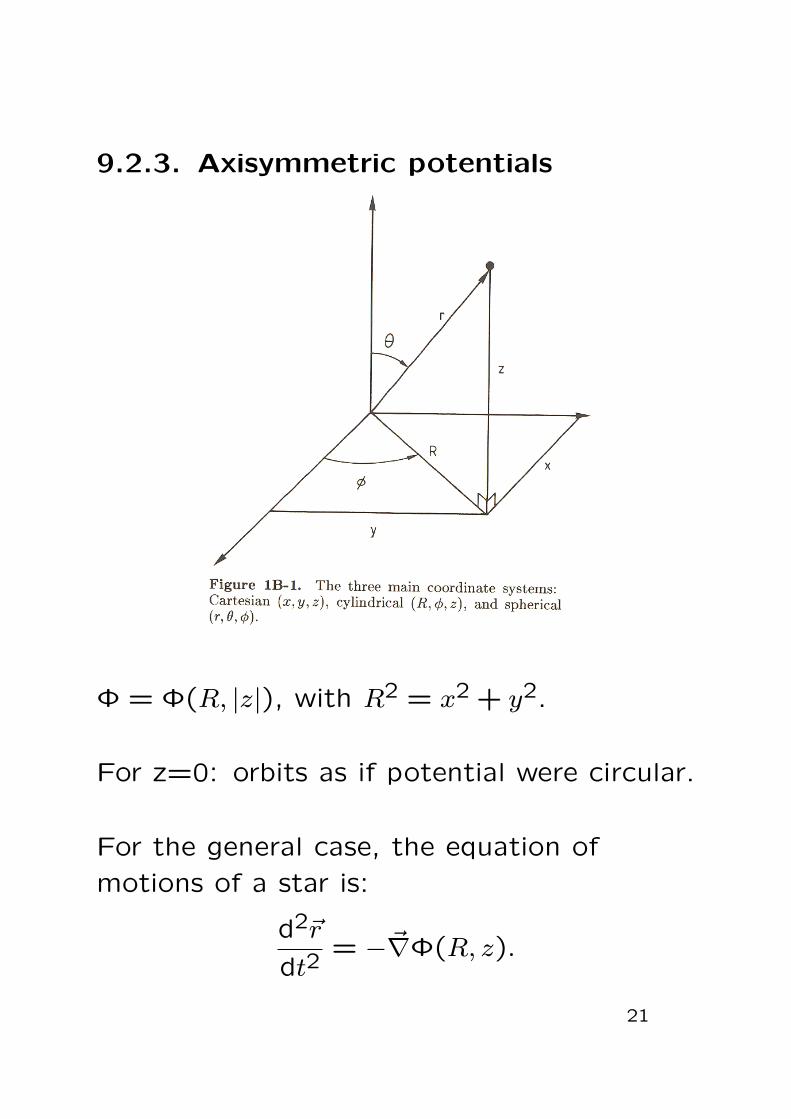
9.2.3. Axisymmetric potentials

Φ = Φ(R, |z|), with R2 = x2 + y2.

For z=0: orbits as if potential were circular.

For the general case, the equation of

motions of a star is:

d2~r

dt2= −~∇Φ(R, z).

21

With ~er, ~eφ, ~ez unit vectors in r, φ and z

direction, we can write:

~r = R~eR + z ~ez,

~∇Φ =∂Φ

∂R~eR +

∂Φ

∂φ~eφ +

∂Φ

∂z~ez with

∂Φ

∂φ= 0.

Using BT (App. B.2), the acceleration d2~rdt2

in cylindrical coordinates can be written as:

d2~r

dt2= (R−Rφ2)~eR + (2Rφ+Rφ)~eφ + z~ez.

Note that:

d

dtLz ≡

d

dtR2φ = 2Rφ+Rφ = 0.

and conclude that the angular momentum

about the z-axis is conserved.

If we use this to eliminate φ, we obtain for

the equation of motions in the ~er and ~ez

directions:

22

d2R

dt2= −

∂Φeff

∂R;

d2z

dt2= −

∂Φeff

∂z

with Φeff = Φ(R, z) +L2z

2R2.

Hence 3D motion can be reduced to motion

in (R,z) plane or meridional plane, under

influence of the effective potential Φeff.

Note that this meridonial plane can rotate.

Application to a logarithmic potential

Recall: the axisymmetric logarithmic

potential (Rc taken to be zero):

Φ(R, z) = 12v

20 ln(R2 +

z2

q2).

Then:

Φeff =1

2v2

0 ln(R2 +z2

q2) +

L2z

2R2.

23

24

Total energy:

E =1

2[R2 + (rφ)2 + z2] + Φ

=1

2(R2 + z2) +

(Φ +

L2z

2R2

)

=1

2(R2 + z2) + Φeff .

Allowed region in meridional plane

Since the kinetic energy is non-negative,

orbits are only allowed in areas where:

Φeff < E. E.g.

Lines of constant Φeff are shown in Figure

3.2. Stars with energy E have zero velocity

at curves of Φeff = E

25

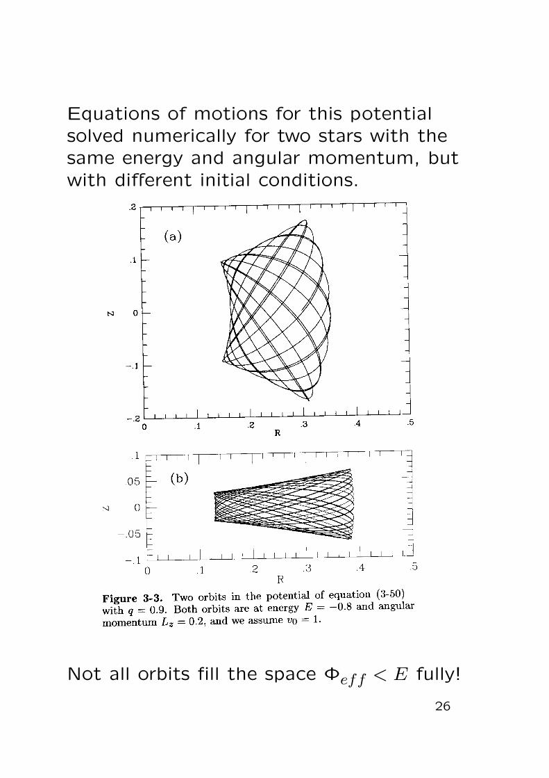
Equations of motions for this potentialsolved numerically for two stars with thesame energy and angular momentum, butwith different initial conditions.

Not all orbits fill the space Φeff < E fully!

26

Two integrals (E,Lz) reduce the

dimensionality of the orbit from 6 to 4 (e.g.

R, z, ψ, vz). Therefore another integral of

motion must play a role → dimensionality

reduced to 3 (e.g. R, z, ψ).

This integral is a non-classical integral of

motion.

27

9.3 A general 3-dimensional potential

Stackel potential: ρ = 1/(1 +m2)2

with m2 = x2

a2 + y2

b2+ z2

c2.

28

29

9.4 Schwarzschild’s method

A simple recipe to build galaxies

• Define density ρ.

• Calculate potential, forces.

• Integrate orbits, find orbital densities ρi.

• Calculate weights wi > 0 such that

ρ =∑

ρiwi.

Examples: build a 2D galaxy in a

logarithmic potential Φ = ln(1 +x2 + y2/a).

30

• As we saw, box orbits void the outerx-axis.

• As we saw, loop orbits void the innerx-axis.

→ both box and loop orbits are needed.

Suppose we have constructed a model.

• What kind of rotation can we expect ?

box orbits: no net rotation.

loop orbits: can rotate either way:positive, negative, or “neutral”.

Hence: The rotation can vary betweenzero, and a maximum rotation Amaximum rotation is obtained if all looporbits rotate the same way.

31

• Is the solution unique ?

box orbits are defined by 2 integrals ofmotion, say the coordinates of the corner

loop orbits have two integrals of motion

Hence, we have two construct a 2dimensional function from thesuperposition of two 2-dimentionalfunctions

ρ(~x, ~y) = wbox(I1, I2)ρbox(I1, I2)+

wloop(I1, I2)ρloop(I1, I2)

The unknown functions are wbox(I1, I2) andwloop(I1, I2). The system isunderdetermined. Hence, many solutionsare possible.

32

9. Homework Assignments:

1) Box orbits are characterized by the fact

they they go through the center, and have

no net angular momentum. Explain how it

comes that they don’t have net angular

momentum, even though a star in a box

orbit has a non-zero angular momentum at

most times.

2) How is it possible that the box orbit

touches the equipotential surface given by

Energy = Φ?

3) Why does a loop orbit not touch that

surface ?

4) Why do we expect virtually no loop

orbits in a homogeneous ellipsoid ?

5) Figure 3-2 (page 24) shows contours

plot for effective potentials related to an

axisymmetric logarithmic potential given on

33

page 23. When does the minimum occur?

What kind of orbit does this minimum

represent?

6) Calculate at least 3 orbits in the

2-dimentional potential

Φ = ln(1 + x2 + y2/2). Do this as follows:

Start the star at a given location (x0,0)

with velocity (0, v0). Calculate the shift in

position at time dt by dt*~v. Calculate the

shift in velocity at time dt by dt*~F . And

keep integrating !

Also plot the equipotential curve where

Energy E = Φ.