827

Motion Planni35. Motion Planning and Obstacle Avoidance

Javier Minguez, Florent Lamiraux, Jean-Paul Laumond

This chapter describes motion planning and ob-stacle avoidance for mobile robots. We will seehow both areas do not share the same modelingbackground. From the very beginning of motionplanning, the research has been dominated bycomputer science. Researchers aim at devisingwell-grounded algorithms with well-understoodcompleteness and exactness properties. The intro-duction of nonholonomic constraints has forcedthese algorithms to be revisited via the intro-duction of differential geometry approaches. Sucha combination has been made possible for certainclasses of systems, so-called small-time control-lable ones. The underlying hypothesis of motionplanning algorithms remains the knowledge ofa global and accurate map of the environment.More than that, the considered system is a for-mal system of equations that does not accountfor the entire physical system: uncertainties inthe world or system modeling are not consid-ered. Such hypotheses are too strong in practice.This is why other complementary researchers haveadopted a parallel, more pragmatic but realis-tic approach to deal with obstacle avoidance. Theproblem here is not to deal with complicatedsystems like a car with multiple trailers. The con-sidered systems are much simpler with respectto their geometric shape. The problem considerssensor-based motion to face the physical issuesof a real system navigating in a real world betterthan motion planning algorithms: how to nav-

igate toward a goal in a cluttered environmentwhen the obstacles to avoid are discovered inreal time? This is the question obstacle avoidanceaddresses.

35.1 Nonholonomic Mobile Robots: WhereMotion Planning Meets Control Theory ... 828

35.2 Kinematic Constraints and Controllability 82935.2.1 Definitions ................................. 82935.2.2 Controllability ............................. 82935.2.3 Example: The Differentially Driven

Mobile Robot .............................. 830

35.3 Motion Planningand Small-Time Controllability .............. 83035.3.1 The Decision Problem .................. 83035.3.2 The Complete Problem ................. 831

35.4 Local Steering Methodsand Small-Time Controllability .............. 83235.4.1 Local Steering Methods that

Account for Small-TimeControllability ............................. 832

35.4.2 EquivalenceBetween Chained-Formedand Feedback-LinearizableSystems ..................................... 834

35.5 Robots and Trailers ............................... 83535.5.1 Differentially Driven Mobile Robots 83535.5.2 Differentially Driven Mobile Robots

Towing One Trailer....................... 83535.5.3 Car-Like Mobile Robots ................ 83535.5.4 Bi-steerable Mobile Robots .......... 83535.5.5 Differentially Driven Mobile Robots

Towing Trailers............................ 83635.5.6 Open Problems ........................... 836

35.6 Approximate Methods ........................... 83735.6.1 Forward Dynamic Programming .... 83735.6.2 Discretization of the Input Space ... 83735.6.3 Input-Based Rapidly Exploring

Random Trees ............................. 837

35.7 From Motion Planningto Obstacle Avoidance ........................... 837

35.8 Definition of Obstacle Avoidance ............ 838

35.9 Obstacle Avoidance Techniques .............. 83935.9.1 Potential Field Methods (PFM) ....... 83935.9.2 Vector Field Histogram (VFH) ......... 840

Part

E35

828 Part E Mobile and Distributed Robotics

35.9.3 The Obstacle Restriction Method(ORM)......................................... 841

35.9.4 Dynamic Window Approach (DWA) . 84235.9.5 Velocity Obstacles (VO).................. 84335.9.6 Nearness Diagram Navigation (ND) 843

35.10Robot Shape, Kinematics, and Dynamicsin Obstacle Avoidance ........................... 84535.10.1 Techniques

that Abstract the Vehicle Aspects ... 845

35.10.2 Techniquesof Decomposition in Subproblems . 846

35.11 Integration Planning – Reaction ............ 84735.11.1 Path Deformation Systems............ 84735.11.2 Tactical Planning Systems ............. 848

35.12 Conclusions, Future Directions,and Further Reading............................. 849

References .................................................. 850

The appearance of mobile robots in the late 1960s

to early 1970s initiated a new research domain: au-

tonomous navigation. It is interesting to notice that the

first navigation systems were published in the very first

International Joint Conferences onArtificial Intelligence

(IJCAI 1969). These systems were based on seminal

ideas which have been very fruitful in the development

of robot motion planning algorithms. For instance, in

1969, the mobile robot Shakey used a grid-based ap-

proach to model and explore the environment [35.1]; in

1977 Jason used a visibility graph built from the corners

of the obstacles [35.2]; in 1979 Hilare decomposed the

environment into collision-free convex cells [35.3].

In the late 1970s, studies of robot manipulators

popularized the notion of configuration space of a me-

chanical system [35.4]. In the configuration space the

piano becomes a point. The motion planning problem

for a mechanical system was thus reduced to find-

ing a path for a point in the configuration space. The

way was open to extend the seminal ideas and to de-

velop new andwell-grounded algorithms (see Latombe’s

book [35.5]).

One decade later, the notion of nonholonomic sys-

tems (also borrowed from mechanics) appeared in the

literature [35.6] on robot motion planning through the

problem of car parking. This problem had not been

solved by the pioneering works on mobile robot nav-

igation. Nonholonomic motion planning then became

an attractive research field [35.7].

Besides this research effort in path planning, work

was initiated in order to make robots move out of their

initially artificial environments where the world was

cylindrical and composed of wooden vertical boards.

Robots started to move in laboratory buildings, with

people walking around. Inaccurate localization, uncer-

tain and incomplete maps of the world, and unexpected

moving or static obstacles made roboticists aware of the

gap between planning a path and executing a motion.

From then on, the domain of obstacle avoidance has

been very active.

The challenge of this chapter is to present both

nonholonomic motion planning (Sects. 35.1–35.6) and

obstacle avoidance (Sects. 35.7–35.10) issues. Sec-

tion 35.11 reviews recent successful approaches that

tend to embrace the whole problem of motion planning

and motion control. These approaches benefit from both

nonholonomic motion planning and obstacle avoidance

methods.

35.1 Nonholonomic Mobile Robots:Where Motion Planning Meets Control Theory

Nonholonomic constraints are nonintegrable linear con-

straints over the velocity space of a system. For

instance, the rolling without slipping constraint of

a differentially driven mobile robot (Fig. 35.1) is

linear with respect to the velocity vector (vector

of linear and angular velocities) of the differen-

tially driven robot and is nonintegrable (it cannot

be integrated into a constraint over the configura-

tion variables). As a consequence, a differentially

driven mobile robot can go anywhere but not fol-

lowing any trajectory. Other types of nonholonomic

constraints arise when considering second-order dif-

ferential equations such as the conservation of inertial

momentum. A number of papers investigate the fa-

mous falling cat problem or free-floating robots in space

(see [35.7] for an overview). This chapter is devoted

Part

E35.1

Motion Planning and Obstacle Avoidance 35.2 Kinematic Constraints and Controllability 829

x

θ

y

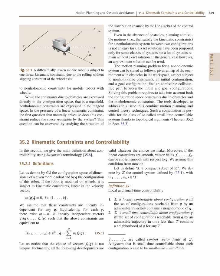
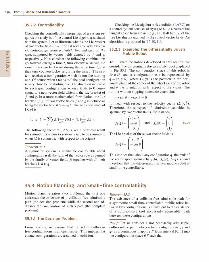
Fig. 35.1 A differentially driven mobile robot is subject to

one linear kinematic constraint, due to the rolling without

slipping constraint of the wheel axis

to nonholonomic constraints for mobile robots with

wheels.

While the constraints due to obstacles are expressed

directly in the configuration space, that is a manifold,

nonholonomic constraints are expressed in the tangent

space. In the presence of a linear kinematic constraint,

the first question that naturally arises is: does this con-

straint reduce the space reachable by the system? This

question can be answered by studying the structure of

the distribution spanned by the Lie algebra of the control

system.

Even in the absence of obstacles, planning admissi-

ble motions (i. e., that satisfy the kinematic constraints)

for a nonholonomic system between two configurations

is not an easy task. Exact solutions have been proposed

only for some classes of systems but a lot of systems re-

mainwithout exact solution. In the general case however,

an approximate solution can be used.

The motion planning problem for a nonholonomic

system can be stated as follows: given a map of the envi-

ronment with obstacles in the workspace, a robot subject

to nonholonomic constraints, an initial configuration,

and a goal configuration, find an admissible collision-

free path between the initial and goal configurations.

Solving this problem requires to take into account both

the configuration space constraints due to obstacles and

the nonholonomic constraints. The tools developed to

address this issue thus combine motion planning and

control theory techniques. Such a combination is pos-

sible for the class of so-called small-time controllable

systems thanks to topological arguments (Theorem 35.2

in Sect. 35.3).

35.2 Kinematic Constraints and Controllability

In this section, we give the main definition about con-

trollability, using Sussman’s terminology [35.8].

35.2.1 Definitions

Let us denote by CS the configuration space of dimen-

sion n of a givenmobile robot and by q the configuration

of this robot. If the robot is mounted on wheels, it is

subject to kinematic constraints, linear in the velocity

vector:

ωi (q)q = 0, i ∈ 1, . . . , k .

We assume that these constraints are linearly in-

dependent for any q. Equivalently, for each q,

there exist m = n − k linearly independent vectors

f1(q), . . . , fm(q) such that the above constraints are

equivalent to

∃(u1, . . . , um) ∈ Rm, q =

m∑

i=1ui fi (q) . (35.1)

Let us notice that the choice of vectors fi (q) is not

unique. Fortunately, all the following developments are

valid whatever the choice we make. Moreover, if the

linear constraints are smooth, vector fields f1, . . . , fm

can be chosen smooth with respect to q. We assume this

condition from now on.

Let us define U, a compact subset of Rm . We de-

note by Σ the control system defined by (35.1), with

(u1, . . . , um) ∈ U

Definition 35.1

Local and small-time controllability

1. Σ is locally controllable about configuration q iff

the set of configurations reachable from q by an

admissible trajectory contains a neighborhood of q,

2. Σ is small-time controllable about configuration q

iff the set of configurations reachable from q by an

admissible trajectory in time less than T contains

a neighborhood of q for any T ,

f1, . . . , fm are called control vector fields of Σ.

A system that is small-time controllable about each

configuration is said to be small-time controllable.

Part

E35.2

830 Part E Mobile and Distributed Robotics

35.2.2 Controllability

Checking the controllability properties of a system re-

quires the analysis of the control Lie algebra associated

with the system. Let us illustrate what is the Lie bracket

of two vector fields in a informal way. Consider two ba-

sic motions: go along a straight line and turn on the

spot, supported by vector fields denoted by f and g,

respectively. Now consider the following combination:

go forward during a time t, turn clockwise during the

same time t, go backward during the same time t, and

then turn counterclockwise during the time t. The sys-

tem reaches a configuration which is not the starting

one. Of course when t tends to 0 the goal configuration

is very close to the starting one. The direction indicated

by such goal configurations when t tends to 0 corre-

spond to a new vector field which is the Lie bracket of

f and g. In a more mathematical formulation, the Lie

bracket [ f, g] of two vector fields f and g is defined as

being the vector field ∂ fg−∂g f . The k-th coordinate of

[ f, g] is

[ f, g][k] =n

∑

i=1(g[i]

∂

∂xi

f [k]− f [i]∂

∂xi

g[k]) .

The following theorem [35.9] gives a powerful result

for symmetric systems (a system is said to be symmetric

when U is symmetric with respect to the origin)

Theorem 35.1

A symmetric system is small-time controllable about

configuration q iff the rank of the vector space spanned

by the family of vector fields fi together with all their

brackets is n at q.

Checking the Lie algebra rank condition (LARC) on

a control system consists of trying to build a basis of the

tangent space from a basis (e.g., a P. Hall family) of the

free Lie algebra spanned by the control vector fields. An

algorithm is proposed in [35.10, 11].

35.2.3 Example: The Differentially DrivenMobile Robot

To illustrate the notions developed in this section, we

consider the differentially driven mobile robot displayed

in Fig. 35.1. The configuration space of this robot is

R2 ×S

1, and a configuration can be represented by

q = (x, y, θ), where (x, y) is the position in the hori-

zontal plane of the center of the wheel axis of the robot

and θ the orientation with respect to the x-axis. The

rolling without slipping kinematic constraint:

−x sin θ + y cos θ = 0

is linear with respect to the velocity vector (x, y, θ).

Therefore, the subspace of admissible velocities is

spanned by two vector fields, for instance:

f1(q)=

cos θ

sin θ

0

and f2(q)=

0

0

1

. (35.2)

The Lie bracket of these two vector fields is

f3(q)=

sin θ

− cos θ

0

.

This implies that, about any configuration q, the rank of

the vector space spanned by f1(q), f2(q), f3(q) is 3 and

therefore that the differentially driven mobile robot is

small-time controllable.

35.3 Motion Planning and Small-Time Controllability

Motion planning raises two problems: the first one

addresses the existence of a collision-free admissible

path (the decision problem) while the second one ad-

dresses the computation of such a path (the complete

problem).

35.3.1 The Decision Problem

From now on, we assume that the set of collision-

free configurations is an open subset. This implies that

contact configurations are assumed in collision.

Theorem 35.2

The existence of a collision-free admissible path for

a symmetric small-time controllable mobile robot be-

tween two configurations is equivalent to the existence

of a collision-free (not necessarily admissible) path

between these configurations.

Proof: Let us consider a not necessarily admissible,

collision-free path between two configurations q1 and

q2 as a continuous mapping Γ from interval [0, 1] intothe configuration space CS such that:

Part

E35.3

Motion Planning and Obstacle Avoidance 35.3 Motion Planning and Small-Time Controllability 831

1. Γ (0)= q1, Γ (1)= q2,

2. for any t ∈ [0, 1], Γ (t) is collision free.

Point 2 implies that, for any t, there exists a neighbor-

hood U(t) of Γ (t) included in the collision-free subset

of the configuration space.

Let us denote by ε(t) the bigger lower bound of

the time to collision of all the trajectories starting from

Γ (t). As the control vector (u1, . . . , um) remains in the

compact set U, ε(t)> 0.

As the system is small-time controllable about Γ (t),

the set reachable from Γ (t) in time less than ε(t) is

a neighborhood of Γ (t) that we denote by V (t).

The collection V (t), t ∈ [0, 1] is an open coveringof the compact set Γ (t), t ∈ [0, 1]. Therefore, we canextract a finite covering: V (t1), . . . , V (tl), where t1 =0< t2 < . . . < tl−1 < tl = 1 such that, for any i between

1 and l −1, V (ti )∩ V (ti+1) 6= ∅. For each i between 1

and l −1, we choose one configuration ri in V (ti )∩V (ti+1). As the system is symmetric, there exists an

admissible collision-free path between q(ti ) and ri and

between ri and q(ti+1). The concatenation of these pathsis a collision-free admissible path between q1 and q2.

35.3.2 The Complete Problem

In the former section, we established that the deci-

sion problem, i. e., determining whether there exists

a collision-free admissible path between two con-

figurations, is equivalent to determining whether the

configurations lie in the same connected component of

the collision-free configuration space. In this section we

present the tools necessary to solve the complete prob-

lem. These tools blend ideas from the classical motion

planning problem addressed in Chap. 5 and from open-

loop control theory, but require specific developments

that we are going to present in the next section. Twomain

approaches have been devised in order to plan admis-

sible collision-free motions for nonholonomic systems.

The first one, proposed by [35.12], exploits the idea

of the proof of Theorem 35.2 by recursively approxi-

mating a not necessarily admissible, collision-free path

by a sequence of feasible paths. The second approach

replaces the local method of probabilistic roadmap

method (PRM) algorithms (Chap. 5) by a local steering

method that connects configuration pairs by admissible

paths.

Both approaches use a steering method. Before

briefly describing them, we give the definition of a local

steering method.

Definition 35.2

A local steering method for system Σ is a mapping

Sloc : CS×CS → C1pw([0, 1], CS) ,

(q1, q2) 7→ Sloc(q1, q2) ,

where Sloc(q1, q2) is a piecewise continuously differen-

tiable curve in CS satisfying the following properties:

1. Sloc(q1, q2) satisfies the kinematic constraints asso-

ciated to Σ,

2. Sloc(q1, q2) connects q1 to q2: Sloc(q1, q2)(0) = q1,

Sloc(q1, q2)(1)= q2 .

Approximationof a Not Necessarily Admissible Path

A not necessarily admissible collision-free path Γ (t),

t ∈ [0, 1] connecting two configurations and a local

steering method Sloc being given, the approximation

algorithm proceeds recursively by calling the function

approximation defined by Algorithm 35.1 with in-

puts Γ , 0, and 1.

Algorithm 35.1

approximation function: inputs are a path Γ and

two abscissas t1 and t2 along this path

if Sloc(Γ (t1), Γ (t2)) collision free then

return Sloc(Γ (t1), Γ (t2))

else

return concat(approximation(Γ ,t1,(t1+t2)/2),approximation(Γ ,(t1+t2)/2,t2))

endif

Sampling-Based Roadmap MethodsMost sampling-based roadmap methods as described

in Chap. 5 can be adapted to nonholonomic systems

by replacing the connection method between pairs of

configurations by a local steering method. This strat-

egy is rather efficient for PRM algorithms. For the rapid

random trees (RRT) method, the efficiency strongly de-

pends on the metric used to choose the nearest neighbor.

The distance function between two configurations needs

to account for the length of the path returned by the local

steeringmethod to connect these configurations [35.13].

Part

E35.3

832 Part E Mobile and Distributed Robotics

35.4 Local Steering Methods and Small-Time Controllability

The approximation algorithm described in the former

section is recursive and raises the completeness ques-

tion: does the algorithm finish in finite time or may it

fail to find a solution?

A sufficient condition for the approximation algo-

rithm to find a solution in a finite number of iterations

is that the local steering method accounts for small-time

controllability.

Definition 35.3

A local steering method Sloc accounts for the small-time

controllability of system Σ iff

For any q ∈ CS, for any neighborhoodU of q,

there exists a neighborhood V of q such that

for any r ∈ V, Sloc(q, r)([0, 1])⊂ U

a)

b) –2

20

2

0

–2

2π

π

0

–2

20

2

0

–2

2π

π

0

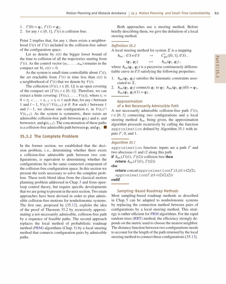
Fig. 35.2 (a) Two perspective views of an RS ball: the set of con-

figurations reachable by a path of length less than a given distance

for Reeds and Shepp car. (b) Perspective views of two DD balls:

the set of configurations reachable by a path of length less than

a given distance for the differentially driven robot. The orientation

θ is represented on the z-axis

In other words, a local steering method accounts for

the small-time controllability of a system if it produces

paths getting closer to the configurations it connects

when these configurations get closer to each other.

This property is also sufficient for probabilistic com-

pleteness of roadmap sampling-based methods.

35.4.1 Local Steering Methods that Accountfor Small-Time Controllability

Constructing a local steering method that accounts for

small-time controllability is a difficult task that has been

achieved only for a few classes of systems. Most mobile

robots studied in the domain of motion planning are

wheeled mobile robots, towing trailers or not.

Steering Using Optimal ControlThe simplest system, namely the differentially driven

robot presented in Sect. 35.2.3 with bounded veloci-

ties or the so-called Reeds and Shepp (RS) [35.14] car

with bounded curvature have the same control vector

fields (35.2). The difference lies in the domain of the

control variables:

• −1≤ u1 ≤ 1, |u2| ≤ |u1| for the RS car,• |u1|+b|u2| ≤ 1 for the differentially driven robot

where b is half of the distance between the right and

left wheels. For these systems, a local steering method

accounting for small-time controllability can be con-

structed using optimal control theory. For any admissible

path defined over an interval I of one of these systems,

we define a length as follows:∫

I

|u1| for RS car ,

∫

I

|u1|+b|u2| for the differentially driven robot .

The length of the shortest path between two con-

figurations defines in both cases a metric over the

configuration space. The synthesis of the shortest paths,

i. e., the determination of the shortest path between

any pair of configurations has been achieved, respec-

tively, by [35.15] for RS car and later by [35.16] for

the differentially driven (DD) robot. Figure 35.2 shows

a representation of the balls corresponding to these

metrics.

Optimal control naturally defines a local steering

method that associates to any pair of configurations,

Part

E35.4

Motion Planning and Obstacle Avoidance 35.4 Local Steering Methods and Small-Time Controllability 833

a shortest path between these configurations. Let us no-

tice that the shortest path is unique between most pairs

of configurations. A general result states that the collec-

tion of balls of radius r > 0 centered about q induced

by nonholonomic metrics constitute an increasing col-

lection of neighborhoods of q the intersection of which

is q. This property directly implies that local steeringmethods based on shortest paths account for small-time

controllability.

The main advantage of optimal control is that it

provides both a local steering method and a distance

metric consistent with the steering method. This makes

the steering methods well suited for path planning al-

gorithms designed for holonomic systems and using

a distance function, such as RRT (Chap. 5) for instance.

Unfortunately, the synthesis of the shortest paths has

been realized only for the two simple systems described

in this section. For more complex systems, the problem

remains open.

The main drawback of the shortest path based steer-

ing methods described in this section is that input

functions are not continuous. This requires an additional

step to compute a time parameterization of the paths be-

foremotion execution.Along this time parameterization,

input discontinuities force the robot to stop, for instance,

to follow two successive arcs of circles of opposite cur-

vature a mobile robot needs to stop between the arcs

of circle in order to ensure continuity of the linear and

angular velocities u1 and u2.

Steering Chained-Form SystemsSome classes of systems can be put into what is called

a chained-form system by a change of variable:

z1 = u1 , (35.3)

z2 = u2 , (35.4)

z3 = z2u1 , (35.5)

...... (35.6)

zn = zn−1u1 . (35.7)

Let us consider the following inputs [35.17]:

u1(t)= a0 +a1 sinωt ,

u2(t)= b0 +b1 cosωt + . . .+bn−2 cos(n −2)ωt .

(35.8)

Let Zstart ∈ Rn be a starting configuration. Each zi (1)

can be computed from the coordinates of Zstart and pa-

rameters (a0, a1, b0, b1, . . . , bn−2). For a given a1 6= 0

and a given configuration Zstart, the mapping from

(a0, b0, b1, b2, b3) to Z(1) is a C1-diffeomorphism at

the origin; the system is then invertible. For n smaller

or equal to 5, the parameters (a0, b0, b1, . . . , bn−2) canbe analytically computed from the coordinates of the

two configurations Zstart and Zgoal. The corresponding

sinusoidal inputs steer the system from Zstart to Zgoal.

The shape of the path only depends on the parame-

ter a1. Each value of a1 thus defines a local steering

method, denoted by Sa1sin. None of these steering meth-

ods account for small-time controllability since, for any

Z ∈ Rn , S

a1sin(Z, Z)([0, 1]) is not reduced to Z. To con-

struct a local steering method accounting for small-time

controllability from the collection of Sa1sin, we need to

make a1 depend on the configurations Z1 and Z2 that

we want to connect:

limZ2→Z1

a1(Z1, Z2)= 0 ,

limZ2→Z1

a0(Z1, Z2, a1(Z

1, Z2))= 0 ,

limZ2→Z1

bi (Z1, Z2, a1(Z

1, Z2))= 0 .

Such a construction is achieved in [35.18].

(y1, y2)

P

l

(x1, x2)

θ

!

Fig. 35.3 A differentially driven robot towing a trailer

hitched on top of the wheel axis of the robot is a feedback-

linearizable system. The linearizing output is the center of

the wheel axis of the trailer. The configuration of the sys-

tem can be reconstructed by differentiating the curve y(s),

where s is an arc-length parameterization, followed by lin-

earizing the output. The orientation of the trailer is given

by τ = arctan(y2/y1). The angle between the robot and the

trailer is given by ϕ = −l arctan(dτ/ds), where l is the

length of the trailer connection

Part

E35.4

834 Part E Mobile and Distributed Robotics

Steering Feedback-Linearizable SystemsThe concept of feedback linearizability (or differential

flatness) was introduced by Fliess et al. [35.19, 20].

A system is said to be feedback linearizable if there

exists an output (i. e., a function of the state, input, and

input derivatives) called the linearizing output, such that

the state and the input of the system are functions of the

linearizing output and its derivatives. The dimension of

the linearizing output is the same as the dimension of

the input.

Let us illustrate this notion with a simple example.

We consider a differentially driven mobile robot towing

a trailer hitched on top of the wheel axis of the robot, as

displayed in Fig. 35.3. The tangent to the curve followed

by the center of the wheel axis of the trailer gives the ori-

entation of the trailer. From the orientation of the trailer

along the curve, we can deduce the curve followed by

the center of the robot. The tangent to the curve fol-

lowed by the center of the robot gives the orientation of

the robot. Thus the linearizing output of this system is

the center of the wheel axis of the trailer. By differen-

tiating the linearizing output twice, we can reconstruct

the configuration of the system.

Feedback linearizability is very interesting for steer-

ing purposes. Indeed, the linearizing output is not subject

to any kinematic constraints. Therefore, if we know the

relation between the state and the linearizing output,

planning an admissible path between two configurations

simply consists of building a curve in Rm , where m is

the dimension of the input with differential constraints

at both ends. This problem can be easily solved using,

for instance, polynomials.

For two input driftless systems likeΣ, the linearizing

output only depends on state q, and the state q depends

on the linearizing output through the parameterization

invariant values, namely, the linearizing output y, the

orientation τ of the vector tangent to the curve followed

by y, and the successive derivatives of τ with respect to

the curvilinear abscissa s.

Thus, the configuration of a two-input feedback-

linearizable driftless system of dimension n can be

represented by a vector (y, τ, τ1, . . . , τn−3) represent-ing the geometric properties of the curve followed by

the linearizing output along an admissible path passing

through the configuration.

Therefore, designing a local steering method for

such a system is equivalent to associating to any pair

of vectors (y1, τ1, τ11 , . . . , τn−3

1 ), (y2, τ2, τ12 , . . . , τn−3

2 )

a curve in the plane starting from y1 and ending at

y2 with orientation of the tangent vector and suc-

cessive derivatives with respect to s, respectively,

equal to τ1, τ11 , . . . , τn−3

1 at the beginning and to

τ2, τ12 , . . . , τn−3

2 at the end. This exercise is relatively

easy using polynomials and transforming the boundary

conditions into linear equations over the coefficients of

the polynomials. However, taking into account small-

time controllability is a little more difficult.

Reference [35.21] propose a flatness-based steer-

ing method built on convex combinations of canonical

curves.

35.4.2 EquivalenceBetween Chained-Formedand Feedback-Linearizable Systems

In the previous section, we proposed methods to steer

feedback-linearizable control systems or systems that

can be put into chained form. We now give a necessary

and sufficient condition for feedback linearizability.

Feedback Linearizability:Necessary and Sufficient Condition

In cite [35.22], Rouchon gives conditions to check

whether a system is feedback linearizable. For two-input

driftless systems a necessary and sufficient condi-

tion is the following: let us define as ∆k, k > 0

the collection of distributions (i. e., the set of vec-

tor fields) iteratively defined by: ∆0 = span f1, f2,∆1 = span f1, f2, [ f1, f2] and ∆i+1 = ∆0 +[∆i , ∆i ]with [∆i , ∆i ] = span[ f, g] , f ∈ ∆i , g ∈ ∆i. A sys-

temwith two-dimensional input is feedback linearizable

iff rank(∆i )= 2+ i.

Example 35.1:The chained-form system. Let us consider

the chained-form system defined by (35.3–35.7). The

control vector fields of this system are:

f1 = (1, 0, z2, . . . , zn−1) f2 = (0, 1, . . . , 0)

rank∆0 = 2. If we compute f3 = [ f1, f2] =(0, 0, 1, 0, . . . , 0), we notice that rank∆1 = 3. By com-

puting fi = [ f1, fi−1] for i up to n we find a sequence

fi = (0, . . . , 0, 1, 0, . . . , 0) where 1 is at position i.

Therefore, rank∆i = 2+ i for i up to n −2 and the

chained-form system is feedback linearizable. This con-

clusion could have been drawn in amore straightforward

way by noticing that the state can be reconstructed from

(z1, z2) and its derivatives. (z1, z2) is thus the linearizing

output of the chained-form system.

Part

E35.4

Motion Planning and Obstacle Avoidance 35.5 Robots and Trailers 835

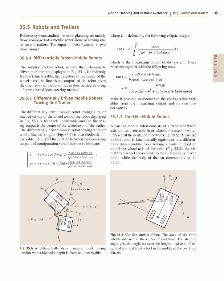
35.5 Robots and Trailers

Robotics systems studied in motion planning are mainly

those composed of a mobile robot alone or towing one

or several trailers. The input of these systems is two

dimensional.

35.5.1 Differentially Driven Mobile Robots

The simplest mobile robot, namely the differentially

driven mobile robot displayed in Fig. 35.1, is obviously

feedback linearizable, the trajectory of the center of the

wheel axis (the linearizing output) of the robot gives

the orientation of the robot. It can thus be steered using

a flatness-based local steering method.

35.5.2 Differentially Driven Mobile RobotsTowing One Trailer

The differentially driven mobile robot towing a trailer

hitched on top of the wheel axis of the robot displayed

in Fig. 35.3 is feedback linearizable and the lineariz-

ing output is the center of the wheel axis of the trailer.

The differentially driven mobile robot towing a trailer

with a hitched kingpin (Fig. 35.4) is also feedback lin-

earizable [35.23] but the relation between the linearizing

output and configuration variables is more intricate:

y1 = x1 −b cos θ + L(φ)b sin θ+a sin(θ+φ)√

a2+b2+2ab cosφ,

y2 = x2 −b sin θ − L(φ)a cos(θ+φ)+b cos θ√

a2+b2+2ab cosφ,

y = (y1, y2) b

a

x = (x1, x2)

θ

φ

Fig. 35.4 A differentially driven mobile robot towing

a trailer with a hitched kingpin is feedback linearizable

where L is defined by the following elliptic integral

L(φ)= ab

φ∫

0

cos σ√

a2 +b2 +2ab cos(σ )dσ ,

which is the linearizing output of the system. These

relations together with the following ones

tan τ =a sin(θ +φ)+b sin θ

b cos θ +a cos(θ +φ),

κ =sin(φ)

cosφ√

a2 +b2 +2ab cosφ+ L(φ) sin(φ)

make it possible to reconstruct the configuration vari-

ables from the linearizing output and its two first

derivatives.

35.5.3 Car-Like Mobile Robots

A car-like mobile robot consists of a fixed rear wheel

axis and two steerable front wheels, the axes of which

intersect at the center of curvature (Fig. 35.5). A car-like

mobile robot is kinematically equivalent to a differen-

tially driven mobile robot towing a trailer hitched on

top of the wheel axis of the robot (Fig. 35.3): the vir-

tual front wheel corresponds to the differentially driven

robot, while the body of the car corresponds to the

trailer.

θ

!

Fig. 35.5 Car-like mobile robot. The axes of the front

wheels intersect at the center of curvature. The steering

angle ϕ is the angle between the longitudinal axis of the

car and a virtual front wheel in the middle of the two front

wheels

Part

E35.5

836 Part E Mobile and Distributed Robotics

θ

α!

Fig. 35.6 Bi-steerable robot. The front and rear wheels are

steerable and there is a relation between the rear steering

angle and the front steering angle: α = f (ϕ)

35.5.4 Bi-steerable Mobile Robots

The bi-steerable mobile robot (Fig. 35.6) is a car with

front and rear steerable wheels and with a relation be-

tween the front and rear steering angles. This system has

been proven to be feedback linearizable in [35.24]. As

for the mobile robot towing a trailer with a hitched king-

pin, the linearizing output is a moving point in the robot

reference frame.

35.5.5 Differentially Driven Mobile RobotsTowing Trailers

Let us consider the differentially driven mobile robot

towing a trailer connected on top of the wheel axis of the

robot, and let us add an arbitrary number of trailers, each

one connected on top of the wheel axis of the previous

one. By differentiating the curve followed by the center

of the last trailer once, we get the orientation of the last

trailer (this orientation coincides with the orientation of

the tangent to the curve). If we know the orientation

and the position of the center of the last trailer along

the path, we can reconstruct the curve followed by the

center of the previous trailer; repeating this reasoning,

we can reconstruct the trajectory of the whole system by

differentiating a sufficient number of times. The system

is therefore feedback linearizable and the linearizing

output is the center of the last trailer.

Fig. 35.7 A truck towing a towbar trailer with hitched king-

pin and a differentially driven mobile robot towing two

trailers with hitched kingpin: two open problems for exact

path planning for nonholonomic systems

Combining the above reasoning with systems

reviewed in this section, we can build hybrid feedback-

linearizable trailer systems. For instance, a differentially

driven mobile robot towing an arbitrary number n

of trailers each one connected on top of the wheel

axis of the previous trailer, except the last trailer with

a hitched kingpin, is feedback linearizable. Simply con-

sider the two last trailers as a feedback-linearizable

system composed of a mobile robot with one trailer

as in Fig. 35.4. The linearizing output of this system

enables us to reconstruct the trajectory of the two

last trailers. The center of trailer n −1 is a lineariz-

ing output for the mobile robot towing the n −1 last

trailers.

35.5.6 Open Problems

Eventually all the systems for which we are able to plan

exact motions between arbitrary pairs of configurations

are included in the large class of feedback-linearizable

systems. We have seen indeed that chained-form sys-

tems are also part of this class. For other systems, no

exact solution has been proposed up to now, for instance,

both systems displayed in Fig. 35.7 are not feedback lin-

earizable. They do not satisfy the necessary condition

of Sect. 35.4.2.

Part

E35.5

Motion Planning and Obstacle Avoidance 35.7 From Motion Planning to Obstacle Avoidance 837

35.6 Approximate Methods

To deal with nonholonomic systems not belonging to

any class of systems for which exact solutions exist,

approximate numerical solutions have been developed.

We review some of these methods in this section.

35.6.1 Forward Dynamic Programming

Barraquand and Latombe propose in [35.25] a dynamic

programming approach to nonholonomic path planning.

Admissible paths are generated by a sequence of con-

stant input values, applied over a fixed interval of time

δt. Starting from the initial configuration the search gen-

erates a tree: the children of a given configuration q are

obtained by setting the input to a constant value and

integrating the differential system over δt. The configu-

ration space is discretized into an array of cells of equal

size (i. e., hyperparallelepipeds). A child q′ of a config-uration q is inserted in the search tree iff the computed

path from q to q′ is collision free and q′ does not belongto a cell containing an already generated configuration.

The algorithm stops when it generates a configuration

belonging to the same cell as the goal (i. e., it does not

necessarily reach the goal exactly).

The algorithm has been proved to be asymptotically

complete with respect to both δt and the size of the cells.

As a brute forcemethod, it remains quite time consuming

in practice. Its main interest is that the search is based on

Dijkstra’s algorithm which allows to take into account

optimality criteria such as the path length or the number

of reversals. Asymptotical optimality to generate the

minimum of reversals is proved for the car-like robot

alone.

35.6.2 Discretization of the Input Space

Divelbiss and Wen propose in [35.26] a method to

produce an admissible collision-free path for a non-

holonomic mobile robot in the presence of obstacles.

They restrict the set of input functions over the subspace

spanned by a Fourier basis over the interval [0, 1]. An in-

put function is thus represented by a finite-dimensional

vector λ. Reaching a goal configuration thus becomes

a nonlinear system of equations, the unknown of which

are the coordinates λi of λ. The authors use the Newton–

Raphsonmethod to find a solution. Obstacles are defined

by inequality constraints over the configuration space.

The path is discretized into N samples. The noncolli-

sion constraint expressed at these sample points yields

inequality constraint over the vector λ. These inequality

constraints are turned into equality constraints through

the function g, defined as:

g(c)=

(1− ec)2 if c > 0

0 if c ≤ 0 .

Reaching a goal configuration while avoiding obstacles

thus becomes a nonlinear system of equations over vec-

tor λ again solved using the Newton–Raphson method.

The method is rather efficient for short maneuvers. The

main difficulty is to tune the order of the Fourier expan-

sion. Long motions in cluttered environments require

a higher order while motion in empty space can be

solved with a low order. The authors do not mention

the problem of numerical instability in the integration of

the dynamic system.

35.6.3 Input-Based Rapidly ExploringRandom Trees

RRT algorithms, described in Chap. 5, can be used

without local steering method to plan paths for non-

holonomic systems. New nodes can be generated from

existing nodes by applying random input functions over

an interval of time [35.27]. The main difficulty consists

in finding a distance function that really accounts for

the distance the system needs to travel to go from one

configuration to another. Moreover, the goal is never ex-

actly reached. This latter drawback can be overcome by

postprocessing the path returned by RRT using a path

deformation method, as described in [35.28].

35.7 From Motion Planning to Obstacle Avoidance

Up to now we have described motion planning tech-

niques. Their objective is to compute a collision-free

trajectory to the target configuration that complies with

the vehicle constraints. They assume a perfect model

of the robot and scenario. The advantage of these tech-

niques is that they provide complete and global solutions

of the problem. Nevertheless, when the surroundings are

unknown and unpredictable, these techniques fail.

Part

E35.7

838 Part E Mobile and Distributed Robotics

A complementary way to address the motion prob-

lem is obstacle avoidance. The objective is to move

a vehicle towards a target location free of collisions with

the obstacles detected by the sensors during motion ex-

ecution. The advantage of reactive obstacle avoidance is

to compute motion by introducing the sensor informa-

tion within the control loop, used to adapt the motion to

any contingency incompatible with initial plans.

The main cost of considering the reality of the world

during execution is locality. In this instance, if global

reasoning is required, a trap situation could occur. De-

spite this limitation, obstacle avoidance techniques are

mandatory to deal with mobility problems in unknown

and evolving surroundings.

Notice that methods have been developed to com-

bine both the global point of view of motion planning

and the local point of view of obstacle avoidance. How

to consider robot perception at the planning level? This

is the so-called sensor-based motion planning. Several

variants exist, such as the BUG algorithms initially in-

troduced in [35.29]. However none of them consider the

practical context of nonholonomic mobile robots.

35.8 Definition of Obstacle Avoidance

Let A be the robot (a rigid object) moving in the

workspace W , whose configuration space is CS. Let

q be a configuration, qt this configuration at time t, and

A(qt) ∈ W the space occupied by the robot in this con-

figuration. In the vehicle there is a sensor, that in qt

measures a portion of the space S(qt) ⊂ W identifying

a set of obstacles O(qt)⊂ W .

Let u be a constant control vector and u(qt) this

control vector applied in qt during time δt. Given u(qt),

the vehicle describes a trajectory qt+δt = f (u, qt, δt),

with δt ≥ 0. Let Qt,T be the set of configurations of the

trajectory followed from qt with δt ∈ [0, T ], a given timeinterval. T > 0 is called the sampling period.

Let F : CS×CS → R+ be a function that evaluates

the progress of one configuration to another.

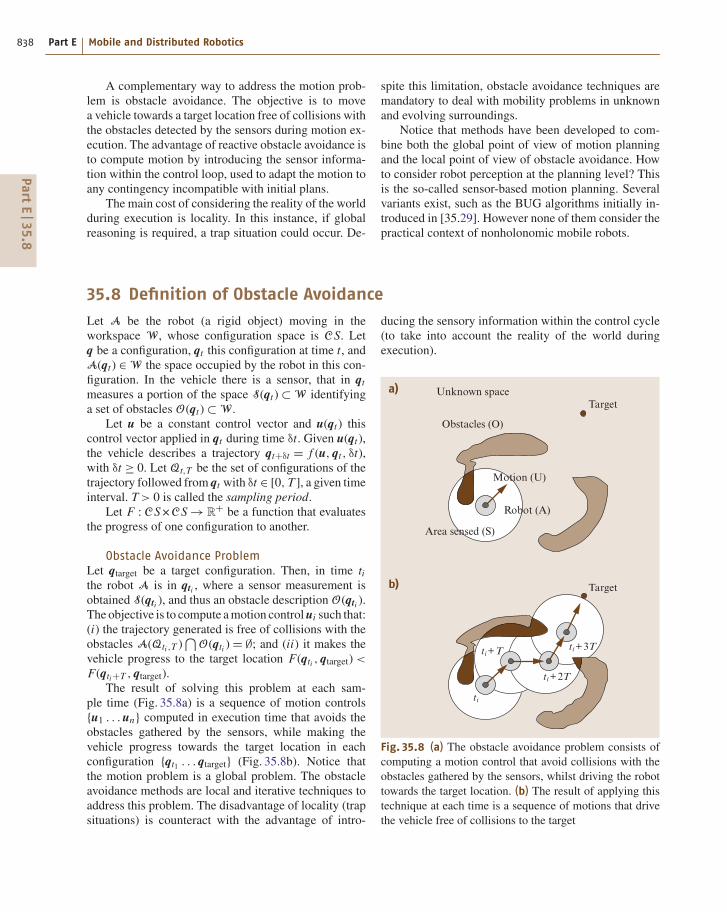
Obstacle Avoidance ProblemLet qtarget be a target configuration. Then, in time tithe robot A is in qti , where a sensor measurement is

obtained S(qti ), and thus an obstacle description O(qti ).

The objective is to compute amotion controlui such that:

(i) the trajectory generated is free of collisions with the

obstacles A(Qti ,T )⋂

O(qti ) = ∅; and (ii) it makes thevehicle progress to the target location F(qti , qtarget) <

F(qti+T , qtarget).

The result of solving this problem at each sam-

ple time (Fig. 35.8a) is a sequence of motion controls

u1 . . . un computed in execution time that avoids theobstacles gathered by the sensors, while making the

vehicle progress towards the target location in each

configuration qt1 . . . qtarget (Fig. 35.8b). Notice that

the motion problem is a global problem. The obstacle

avoidance methods are local and iterative techniques to

address this problem. The disadvantage of locality (trap

situations) is counteract with the advantage of intro-

ducing the sensory information within the control cycle

(to take into account the reality of the world during

execution).

a)

b)

Robot (A)

Area sensed (S)

ti+3T

ti+2T

ti+T

ti

Motion (U)

Unknown space

Target

Target

Obstacles (O)

Fig. 35.8 (a) The obstacle avoidance problem consists of

computing a motion control that avoid collisions with the

obstacles gathered by the sensors, whilst driving the robot

towards the target location. (b) The result of applying this

technique at each time is a sequence of motions that drive

the vehicle free of collisions to the target

Part

E35.8

Motion Planning and Obstacle Avoidance 35.9 Obstacle Avoidance Techniques 839

There are at least three aspects that affect the devel-

opment of an obstacle avoidance method: the avoidance

technique, the type of robot sensor, and the type of

scenario. These subjects correspond to the next three

sections. First, we describe the obstacle avoidance tech-

niques (Sect. 35.9). Second, we discuss the techniques

to adapt a given obstacle avoidance method to work on

a vehicle taking into account the shape, kinematics, and

dynamics (Sect. 35.10). Sensory processing is detailed

in Chaps. 4 and 24. Finally, the usage of an obstacle

avoidance technique on a vehicle in a given scenario

is highly dependent on the scenario nature (static or

dynamic, unknown or known, structured or not, or its

size for example). Usually, this problem is associated

with the integration of planning and obstacle avoidance

(Sect. 35.11).

35.9 Obstacle Avoidance Techniques

Wedescribe here a taxonomyof obstacle avoidance tech-

niques and some representative methods. First there are

two groups: methods that compute the motion in one

step and that do it in more than one. One-step meth-

ods directly reduce the sensor information to a motion

control. There are two types:

• The heuristicmethods were the first techniques used

to generatemotion based on sensors. Themajority of

these works derived from classic planning methods

and will not be described here. See [35.1,29–32] for

some representative works.

• The methods of physical analogies assimilate the

obstacle avoidance to a known physical problem.

We discuss here the potential field methods [35.33,

34]. Other works are variants adapted to uncertain

models [35.35] or that use other analogies [35.36–

38].

Methods with more than one step compute some

intermediate information, which is processed next to

obtain the motion.

• The methods of subset of controls compute an inter-

mediate set of motion controls, and next choose one

of them as a solution. There are two types: (i) meth-

ods that compute a subset of motion directions.

We describe here the vector field histogram [35.39]

and the obstacle restriction method [35.40]. Another

method is presented in [35.41]. (ii) Methods that

compute a subset of velocity controls. We describe

here the dynamic window approach [35.42] and the

velocity obstacles [35.43]. Another method based

on similar principles but developed independently is

the curvature velocity method [35.44].

• Finally, there are methods that compute some high-

level information as intermediate information, which

is translated next inmotion.Wedescribe the nearness

diagram navigation [35.45, 46].

All the methods outlined here have advantages and

disadvantages depending on the navigation context, like

uncertain worlds, motion at high speeds, motion in con-

fined or troublesome spaces, etc. Unfortunately there

is no metric available to measure the performance of

the methods quantitatively. However, for an experi-

mental comparison in terms of their intrinsic problems

see [35.45].

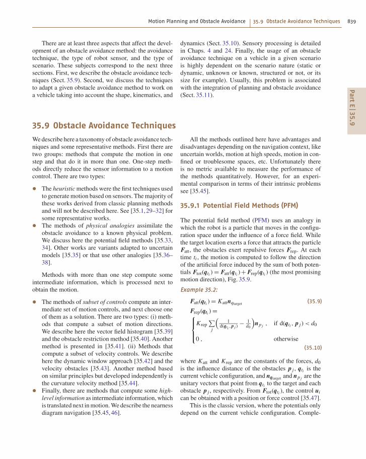
35.9.1 Potential Field Methods (PFM)

The potential field method (PFM) uses an analogy in

which the robot is a particle that moves in the configu-

ration space under the influence of a force field. While

the target location exerts a force that attracts the particle

Fatt, the obstacles exert repulsive forces Frep. At each

time ti , the motion is computed to follow the direction

of the artificial force induced by the sum of both poten-

tials Ftot(qti )= Fatt(qti )+ Frep(qti ) (the most promising

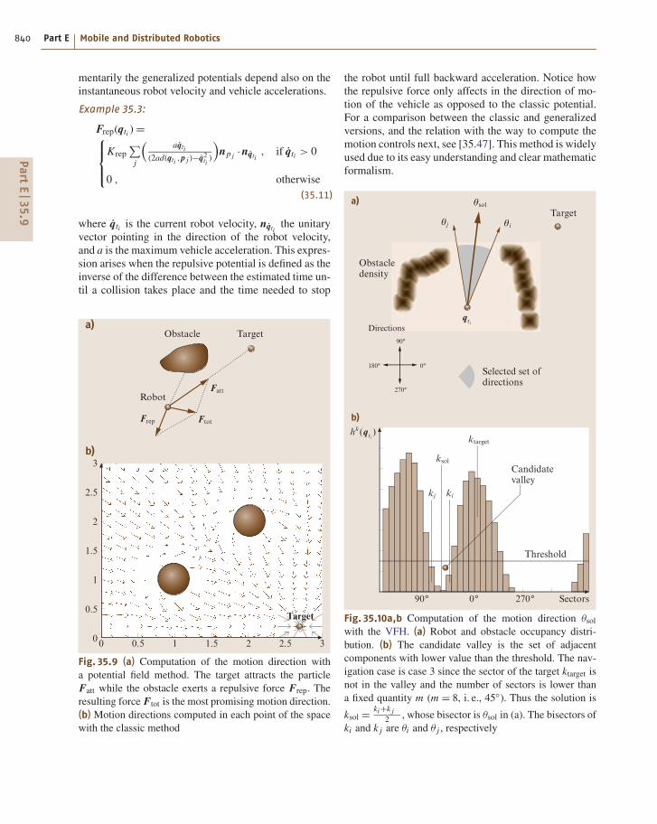
motion direction), Fig. 35.9.

Example 35.2:

Fatt(qti )= Kattnqtarget (35.9)

Frep(qti )=

Krep

∑

j

(

1d(qti

,p j )− 1

d0

)

np j, if d(qti , p j )< d0

0 , otherwise

(35.10)

where Katt and Krep are the constants of the forces, d0is the influence distance of the obstacles p j , qti is the

current vehicle configuration, and nqtarget and np jare the

unitary vectors that point from qti to the target and each

obstacle p j , respectively. From Ftot(qti ), the control ui

can be obtained with a position or force control [35.47].

This is the classic version, where the potentials only

depend on the current vehicle configuration. Comple-

Part

E35.9

840 Part E Mobile and Distributed Robotics

mentarily the generalized potentials depend also on the

instantaneous robot velocity and vehicle accelerations.

Example 35.3:

Frep(qti ) =

Krep

∑

j

(

aqti

(2ad(qti,p j )−q2ti

)

)

np j·nqti

, if qti > 0

0 , otherwise

(35.11)

where qti is the current robot velocity, nqtithe unitary

vector pointing in the direction of the robot velocity,

and a is the maximum vehicle acceleration. This expres-

sion arises when the repulsive potential is defined as the

inverse of the difference between the estimated time un-

til a collision takes place and the time needed to stop

0 0.5 1 1.5 2 2.5 3

Obstacle

Robot

Target

Target

Fatt

FtotFrep

a)

b)3

2.5

2

1.5

1

0.5

0

Fig. 35.9 (a) Computation of the motion direction with

a potential field method. The target attracts the particle

Fatt while the obstacle exerts a repulsive force Frep. The

resulting force Ftot is the most promising motion direction.

(b) Motion directions computed in each point of the space

with the classic method

the robot until full backward acceleration. Notice how

the repulsive force only affects in the direction of mo-

tion of the vehicle as opposed to the classic potential.

For a comparison between the classic and generalized

versions, and the relation with the way to compute the

motion controls next, see [35.47]. This method is widely

used due to its easy understanding and clear mathematic

formalism.

90° 0° 270° Sectors

b)

a)

hk(qti )

kj

ksol

ktarget

Candidatevalley

Threshold

ki

Obstacledensity

Selected set ofdirections

Directions

90°

270°

0°180°

qti

Targetθiθj

θsol

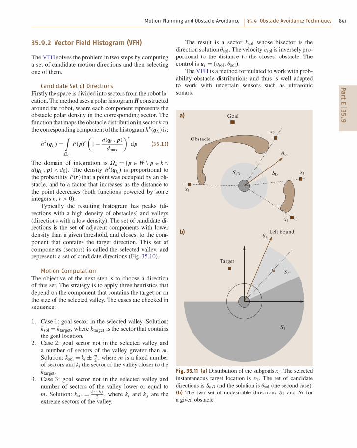
Fig. 35.10a,b Computation of the motion direction θsolwith the VFH. (a) Robot and obstacle occupancy distri-

bution. (b) The candidate valley is the set of adjacent

components with lower value than the threshold. The nav-

igation case is case 3 since the sector of the target ktarget is

not in the valley and the number of sectors is lower than

a fixed quantity m (m = 8, i. e., 45). Thus the solution is

ksol =ki+k j

2, whose bisector is θsol in (a). The bisectors of

ki and k j are θi and θ j , respectively

Part

E35.9

Motion Planning and Obstacle Avoidance 35.9 Obstacle Avoidance Techniques 841

35.9.2 Vector Field Histogram (VFH)

The VFH solves the problem in two steps by computing

a set of candidate motion directions and then selecting

one of them.

Candidate Set of DirectionsFirstly the space is divided into sectors from the robot lo-

cation. Themethod uses a polar histogram H constructed

around the robot, where each component represents the

obstacle polar density in the corresponding sector. The

function thatmaps the obstacle distribution in sector k on

the corresponding component of the histogram hk(qti ) is:

hk(qti )=∫

Ωk

P(p)n(

1−d(qti , p)

dmax

)r

dp (35.12)

The domain of integration is Ωk = p ∈ W \ p ∈ k ∧d(qti , p) < d0. The density hk(qti ) is proportional to

the probability P(r) that a point was occupied by an ob-

stacle, and to a factor that increases as the distance to

the point decreases (both functions powered by some

integers n, r > 0).

Typically the resulting histogram has peaks (di-

rections with a high density of obstacles) and valleys

(directions with a low density). The set of candidate di-

rections is the set of adjacent components with lower

density than a given threshold, and closest to the com-

ponent that contains the target direction. This set of

components (sectors) is called the selected valley, and

represents a set of candidate directions (Fig. 35.10).

Motion ComputationThe objective of the next step is to choose a direction

of this set. The strategy is to apply three heuristics that

depend on the component that contains the target or on

the size of the selected valley. The cases are checked in

sequence:

1. Case 1: goal sector in the selected valley. Solution:

ksol = ktarget, where ktarget is the sector that contains

the goal location.

2. Case 2: goal sector not in the selected valley and

a number of sectors of the valley greater than m.

Solution: ksol = ki ± m2, where m is a fixed number

of sectors and ki the sector of the valley closer to the

ktarget.

3. Case 3: goal sector not in the selected valley and

number of sectors of the valley lower or equal to

m. Solution: ksol =ki+k j

2, where ki and k j are the

extreme sectors of the valley.

The result is a sector ksol whose bisector is the

direction solution θsol. The velocity vsol is inversely pro-

portional to the distance to the closest obstacle. The

control is ui = (vsol, θsol).

The VFH is a method formulated to work with prob-

ability obstacle distributions and thus is well adapted

to work with uncertain sensors such as ultrasonic

sonars.

Goal

Obstacle

Left bound

Target

x2

x3SnD SD

S2

S1

θsol

θL

x4

x1

a)

b)

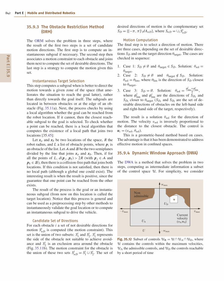
Fig. 35.11 (a) Distribution of the subgoals xi . The selected

instantaneous target location is x2. The set of candidate

directions is SnD and the solution is θsol (the second case).

(b) The two set of undesirable directions S1 and S2 for

a given obstacle

Part

E35.9

842 Part E Mobile and Distributed Robotics

35.9.3 The Obstacle Restriction Method(ORM)

The ORM solves the problem in three steps, where

the result of the first two steps is a set of candidate

motion directions. The first step is to compute an in-

stantaneous subgoal if necessary. The second step then

associates a motion constraint to each obstacle and joins

them next to compute the set of desirable directions. The

last step is a strategy to compute the motion given this

set.

Instantaneous Target SelectionThis step computes a subgoal when is better to direct the

motion towards a given zone of the space (that ame-

liorates the situation to reach the goal latter), rather

than directly towards the goal itself. The subgoals are

located in between obstacles or at the edge of an ob-

stacle (Fig. 35.11a). Next, the process checks by using

a local algorithm whether the goal can be reached from

the robot location. If it cannot, then the closest reach-

able subgoal to the goal is selected. To check whether

a point can be reached, there is a local algorithm that

computes the existence of a local path that joins two

locations [35.45]:

Let xa and xb be two locations of the space, R the

robot radius, and L a list of obstacle points, where pi is

an obstacle of the list. LetA andB be the two semiplanes

divided by the line that joins xa and xb. Then, if for

all the points of L , d(p j , pk) > 2R (with p j ∈ A and

pk ∈ B), then there is a collision-free path that joins both

locations. If this condition is not satisfied, then there is

no local path (although a global one could exist). The

interesting result is when the result is positive, since the

guarantee that one point can be reached from the other

exists.

The result of the process is the goal or an instanta-

neous subgoal (from now on this location is called the

target location). Notice that this process is general and

can be used as a preprocessing step by other methods to

instantaneously validate the goal location or to compute

an instantaneous subgoal to drive the vehicle.

Candidate Set of DirectionsFor each obstacle i a set of not desirable directions for

motion SinD is computed (the motion constraint). This

set is the union of two subsets: Si1 and Si

2. Si1 represents

the side of the obstacle not suitable to achieve avoid-

ance and Si2 is an exclusion area around the obstacle

(Fig. 35.11b). The motion constraint for the obstacle is

the union of these two sets SinD = Si

1 ∪ Si2. The set of

desired directions of motion is the complementary set

SD = [−π, π]\dSnD, where SnD = ∪i SinD.

Motion ComputationThe final step is to select a direction of motion. There

are three cases, depending on the set of desirable direc-

tions SD and on the target direction θtarget. The cases are

checked in sequence:

1. Case 1: SD 6= ∅ and θtarget ∈ SD. Solution: θsol =θtarget.

2. Case 2: SD 6= ∅ and θtarget /∈ SD. Solution:

θsol = θlim, where θlim is the direction of SD closest

to θtarget.

3. Case 3: SD = ∅. Solution: θsol =φllim+φr

lim2

,

where φllim and φr

lim are the directions of SDr and

SDlcloser to θtarget (SDr and SDl

are the set of de-

sirable directions of obstacles on the left-hand side

and right-hand side of the target, respectively).

The result is a solution θsol for the direction of

motion. The velocity vsol is inversely proportional to

the distance to the closest obstacle. The control is

ui = (vsol, θsol).

This is a geometric-based method based on cases.

The advantage is that it has been demonstrated to address

effective motion in confined spaces.

35.9.4 Dynamic Window Approach (DWA)

The DWA is a method that solves the problem in two

steps, computing as intermediate information a subset

of the control space U. For simplicity, we consider

UA

UD

U

wmax

Currentvelocity(υ0,w0)

Nonadmissible

–wmax

υmax–υmax

Fig. 35.12 Subset of controls UR = U∩UA∩UD, where

U contains the controls within the maximum velocities,

UA the admissible controls, andUD the controls reachable

by a short period of time

Part

E35.9

Motion Planning and Obstacle Avoidance 35.9 Obstacle Avoidance Techniques 843

a motion control as translational and rotational velocity

(v, w). U is defined by:

U = (v, w) ∈ R2\ v ∈ [−vmax, vmax]

∧ w ∈ [−wmax, wmax] . (35.13)

Set of Candidate ControlsThe candidate set of controls UR contains the controls

that (i) are within the maximum velocities of the vehicle

U; (ii) generate safe trajectories UA; and (iii) can be

reached within a short period of time given the vehicle

accelerations UD. The set UA contains the admissible

controls. These controls can be canceled before collision

by applying the maximum deceleration (av, aw):

UA = (v, w) ∈ U|v ≤√

2dobsav ∧w ≤√

2θobsaw ,

(35.14)

where dobs and θobs are the distance to the obstacle and

the orientation of the tangent to the trajectory over the

obstacle, respectively. The set UD contains the reach-

able controls in a short period:

UD = (v, w) ∈ U\ v ∈ [v0 −avT, v0 +avT ]∧ w ∈ [w0 −awT, w0 +awT ] , (35.15)

where qti = (v0, w0) is the current velocity.

The resulting subset of controls is (Fig. 35.12):

UR = U∩UA∩UD . (35.16)

Motion ComputationThe next step is to select one control ui ∈ UR. The

problem is set out as the maximization of an objective

function:

G(u)= α1 ·Goal(u)+α2 ·Clearance(u)+α3 ·Velocity(u) . (35.17)

This function is a compromise among Goal(u),

which favors velocities that offer progress to the goal,

Clearance(u), which favors velocities far from the ob-

stacles, and Velocity(u) that favors high speeds. The

solution is the control ui that maximizes this function.

TheDWAsolves the problem in the control space us-

ing information of the vehicle dynamics, thus themethod

is well adapted to work on vehicles with slow dynamic

capabilities or that work at high speeds.

35.9.5 Velocity Obstacles (VO)

The velocity obstacles (VO) method solves the problem

in two steps, by computing as intermediate information

a subset of the U. The framework is the same as for

the DWA method. The difference is that the computa-

tion of the set of safe trajectories UA takes into into

account the velocity of the obstacles, which is described

next.

Let vi be the velocity of obstacle i (that enlargedwith

the vehicle radius occupies an area Bi ) and u a given

vehicle control. The set of colliding relative velocities is

called the collision cone:

CCi =

ui

∣

∣

∣λi

⋂

Bi 6= ∅

, (35.18)

where λi is the direction of the unitary vector ui = ui −vi . The velocity obstacle is this set in a common absolute

system of reference:

VOi = CCi ⊕vi , (35.19)

where the ⊕ is the Minkowski vector sum. The set of

unsafe trajectories is the union of the velocity obstacles

for each moving obstacle UA = ∪i VOi (Fig. 35.13).

The advantage of this method is that it takes into

account the velocity of the obstacles and thus is well

suited to dynamic scenarios.

35.9.6 Nearness Diagram Navigation (ND)

This method is more a methodology to design obstacle

avoidance methods rather than a method in itself. The

ND is an obstacle avoidance method obtained with a ge-

ometric implementation following this methodology.

The idea behind this approach is to employ a divide-

VO1

VO2

B2

B1

Robot

υ2

υ1

Fig. 35.13 The subset of controls that are not safe

UA = VO1∪ VO2. A control vector out of this set generates

a collision free-motion with the moving obstacles

Part

E35.9

844 Part E Mobile and Distributed Robotics

Target

Securitydistance

Area of motion

Obstacles

Robot location

Situations

Obstacleinformation

Goal location

Decision tree

Goalin motionregion

Widemotionregion

Yes

No

Yes

Goalin motionregion

No

Obstaclesin securityzone

No

Yes

No

Yes

Obs. 2sides of motion

region

No

Yes

HSWR HSWR

HSNR HSNR

HSGR HSGR

LS1 LS1

LS2 LS2

LSGR LSGR

Actions

Ds

θdisc

θsolα

Motion

commands

(υ, w)

a) b)

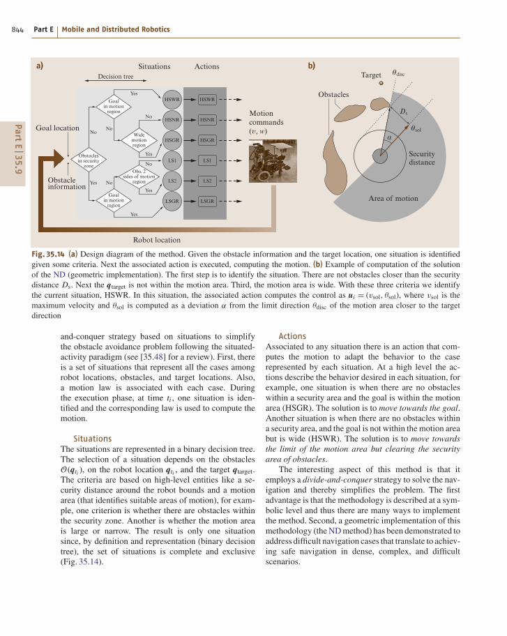
Fig. 35.14 (a) Design diagram of the method. Given the obstacle information and the target location, one situation is identified

given some criteria. Next the associated action is executed, computing the motion. (b) Example of computation of the solution

of the ND (geometric implementation). The first step is to identify the situation. There are not obstacles closer than the security

distance Ds. Next the qtarget is not within the motion area. Third, the motion area is wide. With these three criteria we identify

the current situation, HSWR. In this situation, the associated action computes the control as ui = (vsol, θsol), where vsol is the

maximum velocity and θsol is computed as a deviation α from the limit direction θdisc of the motion area closer to the target

direction

and-conquer strategy based on situations to simplify

the obstacle avoidance problem following the situated-

activity paradigm (see [35.48] for a review). First, there

is a set of situations that represent all the cases among

robot locations, obstacles, and target locations. Also,

a motion law is associated with each case. During

the execution phase, at time ti , one situation is iden-

tified and the corresponding law is used to compute the

motion.

SituationsThe situations are represented in a binary decision tree.

The selection of a situation depends on the obstacles

O(qti ), on the robot location qti , and the target qtarget.

The criteria are based on high-level entities like a se-

curity distance around the robot bounds and a motion

area (that identifies suitable areas of motion), for exam-

ple, one criterion is whether there are obstacles within

the security zone. Another is whether the motion area

is large or narrow. The result is only one situation

since, by definition and representation (binary decision

tree), the set of situations is complete and exclusive

(Fig. 35.14).

ActionsAssociated to any situation there is an action that com-

putes the motion to adapt the behavior to the case

represented by each situation. At a high level the ac-

tions describe the behavior desired in each situation, for

example, one situation is when there are no obstacles

within a security area and the goal is within the motion

area (HSGR). The solution is to move towards the goal.

Another situation is when there are no obstacles within

a security area, and the goal is not within the motion area

but is wide (HSWR). The solution is to move towards

the limit of the motion area but clearing the security

area of obstacles.

The interesting aspect of this method is that it

employs a divide-and-conquer strategy to solve the nav-

igation and thereby simplifies the problem. The first

advantage is that the methodology is described at a sym-

bolic level and thus there are many ways to implement

the method. Second, a geometric implementation of this

methodology (theNDmethod) has been demonstrated to

address difficult navigation cases that translate to achiev-

ing safe navigation in dense, complex, and difficult

scenarios.

Part

E35.9

Motion Planning and Obstacle Avoidance 35.10 Robot Shape, Kinematics, and Dynamics in Obstacle Avoidance 845

35.10 Robot Shape, Kinematics, and Dynamics in Obstacle Avoidance

There are three aspects of the vehicle that have to be

taken into account during the obstacle avoidance pro-

cess: shape, kinematics, and dynamics. The shape and

the kinematics together form a geometric problem that

involves the representation of the vehicle configurations

in collision given the admissible trajectories Qt,∞. The

–3 –2 –1 0

Goal

Target

2

Obstacles

(υ0, w0)

RCARM

RCpARM

qpsol

!sol

CNApARM

Y

X

1 2 3

a)

b)

3

2

1

0

–1

–2

–3

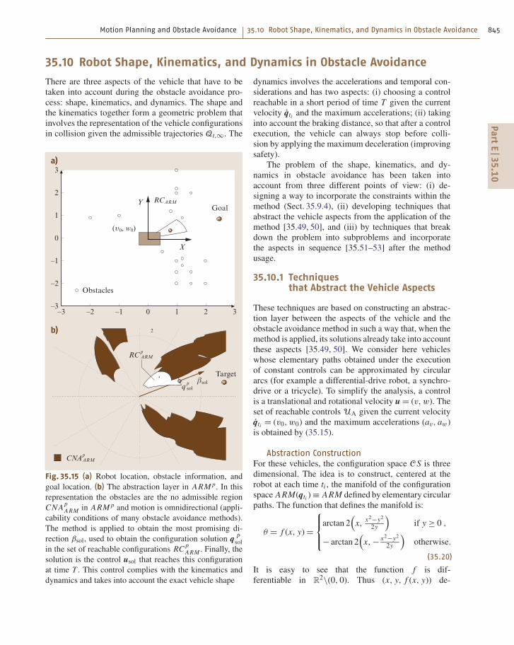
Fig. 35.15 (a) Robot location, obstacle information, and

goal location. (b) The abstraction layer in ARM p. In this

representation the obstacles are the no admissible region

CNAp

ARM in ARM p and motion is omnidirectional (appli-

cability conditions of many obstacle avoidance methods).

The method is applied to obtain the most promising di-

rection βsol, used to obtain the configuration solution qp

sol

in the set of reachable configurations RCp

ARM . Finally, the

solution is the control usol that reaches this configuration

at time T . This control complies with the kinematics and

dynamics and takes into account the exact vehicle shape

dynamics involves the accelerations and temporal con-

siderations and has two aspects: (i) choosing a control

reachable in a short period of time T given the current

velocity qti and the maximum accelerations; (ii) taking

into account the braking distance, so that after a control

execution, the vehicle can always stop before colli-

sion by applying the maximum deceleration (improving

safety).

The problem of the shape, kinematics, and dy-

namics in obstacle avoidance has been taken into

account from three different points of view: (i) de-

signing a way to incorporate the constraints within the

method (Sect. 35.9.4), (ii) developing techniques that

abstract the vehicle aspects from the application of the

method [35.49, 50], and (iii) by techniques that break

down the problem into subproblems and incorporate

the aspects in sequence [35.51–53] after the method

usage.

35.10.1 Techniquesthat Abstract the Vehicle Aspects

These techniques are based on constructing an abstrac-

tion layer between the aspects of the vehicle and the

obstacle avoidance method in such a way that, when the

method is applied, its solutions already take into account

these aspects [35.49, 50]. We consider here vehicles

whose elementary paths obtained under the execution

of constant controls can be approximated by circular

arcs (for example a differential-drive robot, a synchro-

drive or a tricycle). To simplify the analysis, a control

is a translational and rotational velocity u = (v, w). The

set of reachable controls UA given the current velocity

qti = (v0, w0) and the maximum accelerations (av, aw)

is obtained by (35.15).

Abstraction ConstructionFor these vehicles, the configuration space CS is three

dimensional. The idea is to construct, centered at the

robot at each time ti , the manifold of the configuration

space ARM(qti )≡ ARM defined by elementary circular

paths. The function that defines the manifold is:

θ = f (x, y)=

arctan 2(

x,x2−y2

2y

)

if y ≥ 0 ,

− arctan 2(

x, − x2−y2

2y

)

otherwise.

(35.20)

It is easy to see that the function f is dif-

ferentiable in R2\(0, 0). Thus (x, y, f (x, y)) de-

Part

E35.1

0

846 Part E Mobile and Distributed Robotics

fines a two-dimensional manifold in R2 ×S

1 when

(x, y) ∈ R2\(0, 0). This manifold ARM contains all the

configurations that can be reached at each step of the

obstacle avoidance.

Next, in the ARM one computes the exact region of

the configurations in collision COARM given any shape

of the robot (i. e., obstacle representation in the mani-

fold). Given an obstacle point (x p, yp) and a point of

the robot bounds (xr , yr ), a point (xs, ys) of the COARM

boundary is obtained by

xs = (x f + xi ) a ,

ys = (y f − yi ) a , (35.21)

with

a =[(y2f − y2i )+ (x2f − x2i )][(y f − yi )

2 + (x f − xi )2]

(y f − yi )4 +2(x2f + x2i )(y f − yi )2 + (x2f − x2i )2

.

This result is used to map the robot bounds for all ob-

stacles in the manifold, computing the exact shape of

COARM . Next, one computes the nonadmissible con-

figurations CNAARM in the manifold ARM, which

correspond to configurations where, once reached at

a given velocity in time T , the vehicle cannot be

stopped by applying the maximum deceleration with-

out collision (i. e., there is not enough braking distance).

These regions CNAARM are the COARM enlarged

by a magnitude that depends on the maximum vehi-

cle accelerations. The set of configurations reachable

RCARM by controls reachable in a short period of

time UA is also computed in the ARM. Finally,

a change of coordinates is applied to ARM, lead-

ing to ARM p; its effect is that elementary circular

paths become straight segments in the manifold. As

a consequence, the problem is now to move an om-

nidirectional point in a bidimensional space free of any

constraint.

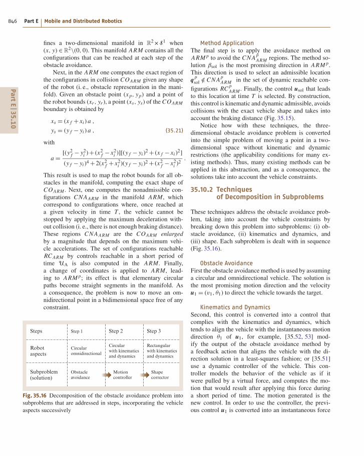
Steps

Robotaspects

Subproblem(solution)

Circular

omnidirectional

Obstacle

avoidance

Circular

with kinematics

and dynamics

Motion

controller

Rectangular

with kinematics

and dynamics

Shape

corrector

Step 1 Step 2 Step 3

Fig. 35.16 Decomposition of the obstacle avoidance problem into

subproblems that are addressed in steps, incorporating the vehicle

aspects successively

Method ApplicationThe final step is to apply the avoidance method on

ARM p to avoid the CNApARM regions. The method so-

lution βsol is the most promising direction in ARM p.

This direction is used to select an admissible location

qp

sol /∈ CNApARM in the set of dynamic reachable con-

figurations RCp

ARM . Finally, the control usol that leads

to this location at time T is selected. By construction,

this control is kinematic and dynamic admissible, avoids

collisions with the exact vehicle shape and takes into

account the braking distance (Fig. 35.15).

Notice how with these techniques, the three-

dimensional obstacle avoidance problem is converted

into the simple problem of moving a point in a two-

dimensional space without kinematic and dynamic

restrictions (the applicability conditions for many ex-

isting methods). Thus, many existing methods can be

applied in this abstraction, and as a consequence, the

solutions take into account the vehicle constraints.

35.10.2 Techniquesof Decomposition in Subproblems

These techniques address the obstacle avoidance prob-

lem, taking into account the vehicle constraints by

breaking down this problem into subproblems: (i) ob-

stacle avoidance, (ii) kinematics and dynamics, and

(iii) shape. Each subproblem is dealt with in sequence

(Fig. 35.16).

Obstacle AvoidanceFirst the obstacle avoidance method is used by assuming

a circular and omnidirectional vehicle. The solution is

the most promising motion direction and the velocity

u1 = (v1, θ1) to direct the vehicle towards the target.

Kinematics and DynamicsSecond, this control is converted into a control that

complies with the kinematics and dynamics, which

tends to align the vehicle with the instantaneous motion

direction θ1 of u1, for example, [35.52, 53] mod-

ify the output of the obstacle avoidance method by

a feedback action that aligns the vehicle with the di-

rection solution in a least-squares fashion; or [35.51]

use a dynamic controller of the vehicle. This con-

troller models the behavior of the vehicle as if it

were pulled by a virtual force, and computes the mo-

tion that would result after applying this force during

a short period of time. The motion generated is the

new control. In order to use the controller, the previ-

ous control u1 is converted into an instantaneous force

Part

E35.1

0

Motion Planning and Obstacle Avoidance 35.11 Integration Planning – Reaction 847

F = (θ1, Fmaxv1

vmax) input of the controller, that com-

putes a control u2 that complies with the kinematic and

dynamics.

ShapeThe final step is to ensure that the control u2 obtained in

the previous step avoids collisions with the exact shape

of the vehicle. To do this, a shape corrector is used to

check collisions by dynamic simulation of the control. If

there is a collision, the set of reachable controls (35.15) is

explored until a collision-free control is found. The result

of this process is a motion control ui that guarantees

obstacle avoidance and complies with the kinematics

and dynamics of the vehicle.

35.11 Integration Planning – Reaction

In this section we show how the obstacle avoidance

methods are integrated into real systems. On the one

hand, obstacle avoidance methods are local techniques

to address the motion problem. Thus, they are doomed

to fall into local minima that translates in trap situations

or cyclic motions. This reveals the necessity of more-

global reasoning. On the other hand, motion planning

techniques compute a geometric path free of collisions

that guarantees global convergence. However, when the

scenarios are unknown and evolve, these techniques fail,

since the precomputed paths will almost surely collide

with obstacles. It seems clear that one key aspect to build

a motion system is to combine the best of both worlds:

the global knowledge given by motion planning and the

reactivity of obstacle avoidance methods.

The most extended ways to specify the interaction

between the deliberation and reaction are: (i) to pre-

compute a path to the target, which is then deformed

during execution as a function of changes in the scenario

obtained from sensor information (path deformation sys-

tems), for example, [35.54–56]. (ii) To use a planner at

a high frequency with a tactical role, leaving the degree

of execution to the reactor [35.57–62].

35.11.1 Path Deformation Systems

The elastic bandsmethod initially assumes the existence

of a geometric path to the target location (computed by

a planner). The path is assimilatedwith a band, subjected

to two types of forces: an inner contraction force and an

external force. The inner force simulates the tension of

a strip and maintains the stress. The external force is

exerted by the obstacles and moves the band away from

them. During execution, new obstacles produce forces

that move the band away from them, guarantying their

avoidance. These methods are described in Chap. 5 of

this book.

An extension of the method of path deformation

has been proposed in [35.56] for nonholonomic sys-

tems. Even though the objective is the same as for

mobile robots without kinematic constraints (avoiding

obstacles while following a trajectory), the concepts

are completely different. The trajectory Γ of a non-

holonomic system is completely defined by an initial

configuration Γ (0) and the value of the input function

u ∈ C1(I, Rm), where I is an interval. The trajectory de-

formation method for a nonholonomic system is thus

based on the perturbation of the input function of

the current trajectory in order to achieve three objec-

tives:

1. keeping the nonholonomic constraints satisfied

2. getting away from obstacles detected online by on-

board sensors

3. keeping unchanged the initial and last configurations

of the trajectory after deformation

Perturbing the input function of Γ , by a vector-

valued input perturbation v ∈ C1(I, Rm) yields a trajec-

tory deformation η ∈ C1(I, Rn):

u ← u+ τv ⇒ Γ ← Γ + τη , (35.22)

where τ is a positive asymptotically small real number.

As an approximation of order one, the relation between

u and η is given by the linearized system, which we do

not express here.

Obstacle Potential FieldObstacles are taken into account by defining a potential

field over the configuration space, which increases when

the robot gets closer to obstacles. This potential field is

lifted into the space of trajectories by integration along

the trajectory of the configuration potential value.

Discretization of the Input SpaceThe spaceC1(I, R

m) of input perturbations is an infinite-

dimensional vector space. The choice of an input

perturbation is restricted to a finite-dimensional sub-

Part

E35.1

1

848 Part E Mobile and Distributed Robotics

Fig. 35.17 A differentially driven mobile robot towing a trailer,

applying the trajectory deformation algorithm to avoid obstacles

detected online

space spanned by p arbitrary test functions, e1, . . . ,ep,

where p is a positive integer. An input perturbation:

u =∑p

i=1 λiei is thus defined by a vector λ ∈ Rp. The

variation of the trajectory potential is linear with respect

to λ.

Boundary ConditionsThe boundary conditions consist of applying a trajectory

perturbation equal to zero at both ends of the interval I

that is linear with respect to λ. It is therefore easy to find

a vector λ that makes the potential decrease and that

satisfies the boundary conditions.

Nonholonomic Constraint DeviationThe approximation of order one in the relation be-

tween the input perturbation and trajectory deformation

induces a side effect: after a few iterations, the nonholo-

nomic constraints are not satisfied anymore. This side

effect is corrected by considering an augmented system

with n control vector fields f1, . . . , fn spanning Rn for

each configuration and by keeping the input components

Planning

Modeling

Obstacleavoidance

Sensors Controller

Robot

Action

– motion

Perception

– laser scan

– odemetry

Fig. 35.18 Overview of the motion system

um+1 to un along the additional vector fields as close as

possible to zero.

Figure 35.17 shows an example of the trajectory de-

formation algorithm applied to a nonholonomic system.

35.11.2 Tactical Planning Systems

Tactical planning systems recompute a path to the target

location at a high frequency, and use the main course

to advise the obstacle avoidance module. The design

of these motion systems involves the synthesis of (at

least) three functionalities: the construction of a model,

deliberative planning, and obstacle avoidance. Themod-

Obstacle

Tacticalplanning

Reactivemotion

Free

a)

b)

Fig. 35.19 (a) Snapshot of an experiment carried out with

the motion system described working on a wheelchair robot

equipped with a planar range laser sensor. (b) Information

of the motion system at a given time: current accumulated

map of the scenario, the path computed with the planner

and tactical direction of motion, and the solution of the

reactive obstacle avoidance method

Part

E35.1

1

Motion Planning and Obstacle Avoidance 35.12 Conclusions, Future Directions, and Further Reading 849

eler constructs a representation base for deliberation and

memory for the reactive behavior. The planner generates

global plans that are used as tactics to guide the obsta-

cle avoidancemodule, which generates the local motion.

Below we give a perspective of the three functionalities

and three possible tools to implement them [35.62].

Model Builder ModuleThe construction of a model of the environment (to in-

crease the spatial domain of the planning and used as

a local memory for obstacle avoidance): one possibil-

ity is to use a binary occupancy grid that is updated

whenever a new sensory measurement is available, and

to employ a scan matching technique [35.63, 64] to im-

prove the vehicle odometry before integrating any new

measure in the grid.

Planner ModuleExtraction of the connectivity of the free space (used

to avoid the cyclical motions and trap situations):

a good choice is a dynamic navigation function such

as D∗ [35.65, 66]. The idea behind the planner is to fo-cus the search locally in the areas where the changes

in the scenario structure have occurred and affect the

computation of the path. The planner avoids the lo-

cal minima and is computationally very efficient for

real-time implementations.

Obstacle Avoidance ModuleComputation of the collision-free motion: any of the

methods described in this chapter could be used. One

possibility is the ND method (Sect. 35.9.6) since it has

been demonstrated to be very efficient and robust in

environments with little space to manoeuvre.

Globally the system works as follows (Fig. 35.18):

given a laser scan and the odometry of the vehicle, the

model builder incorporates this information into the ex-

isting model. Next, the information about changes in

obstacle and free space in the model is used by the plan-

ner module to compute the course to follow to reach the

goal. Finally, the avoidancemodule uses the information

about the obstacles contained in the grid and informa-

tion from this tactical planner to generate the motion

(to drive the vehicle free of collisions towards the goal).

The motion is executed by the vehicle controller and

the process restarts with a new sensorial measurement.

It is important to stress that the three modules should

work synchronously within the perception–action cy-

cle for consistency reasons. The advantage of these

systems is that the synergy of the modules allows the

avoidance of trap situations and cyclic motions (the lim-

itations associated with the local nature of the avoidance

methods).

Figure 35.19 shows a snapshot of an experiment

carried out with this motion system.

35.12 Conclusions, Future Directions, and Further Reading

The algorithmic tools presented in this chapter show that

motion planning and obstacle avoidance research tech-

niques have reached a level of maturity that allow their

transfer onto real platforms. Today, several indoor mo-

bile robots use obstacle avoidance techniques on a daily

basis to guide visitors inmuseums. Outdoor applications

still require some developments in terms of perception

and modeling. For these applications, 3-D sensing capa-

bilities are necessary to model the environment but also

to detect obstacles. As an example, several car manu-

facturer are working on parallel parking assistance. The

difficult point of this application is to build a model

of a parking spot from 3-D data in a great variety of

environments.

The grand challenge of autonomous motion in mo-

bile robots consists today of integrating techniques

from different robotics research domains in order to

plan and execute motions for very complex systems

such as humanoid robots. Integration in the sense that

different software components need to work together

on a machine but also in a scientific meaning: the

classical motion planning formulation with configu-

ration variables that locate the robot with respect to

a global reference frame does not fit partially known

environments with imprecise maps. Robotic tasks like

motion need to be specified with respect to land-

marks of the environment. For instance, grasping an

object is by definition a motion specified with re-

spect to the position of the object. Very little has

been done to design a general framework in this

direction.

Useful complementary readings on motion plan-

ning and obstacle avoidance for mobile robots are

[35.5, 67–69].

Part

E35.1

2

850 Part E Mobile and Distributed Robotics

References

35.1 N.J. Nilson: A mobile automaton: an application ofartificial intelligence techniques, 1st Int. Joint Conf.Artif. Intell. (1969) pp. 509–520

35.2 A. Thompson: The navigation system of the JPLrobot, 5th Int. Joint Conf. Artif. Intell. (Cambridge1977) pp. 749–757

35.3 G. Giralt, R. Sobek, R. Chatila: A multi-level plan-ning and navigation system for a mobile robot: afirst approach to Hilare, 6th Int. Joint Conf. Artif.Intell. (Tokyo 1979) pp. 335–337

35.4 T. Lozano-Pérez: Spatial planning: a configurationspace approach, IEEE Trans. Comput. 32(2), 108–120(1983)

35.5 J.C. Latombe: Robot Motion Planning (Kluwer Aca-demic, Dordredt 1991)

35.6 J.P. Laumond: Feasible trajectories for mobilerobots with kinematic and environment con-straints. In: Intelligent Autonomous Systems, ed.by F.C.A. Groen (L.O. Hertzberger, Amsterdam 1987)pp. 346–354

35.7 Z. Li, J.F. Canny: Nonholonomic Motion Planning

(Kluwer Academic, Dordredt 1992)35.8 H. Sussmann: Lie brackets, real analyticity and ge-

ometric control. In: Differential Geometric Control

Theory, Progress in Mathematics, Vol. 27, ed. byR. Brockett, R. Millman, H. Sussmann (MichiganTechnological Univ., Birkhauser 1982) pp. 1–116

35.9 H.J. Sussmann, V. Jurdjevic: Controllability of non-linear systems, J. Differ. Equ. 12, 95–116 (1972)

35.10 J.P. Laumond: Singularities and topological aspectsin nonholonomic motion planning. In: Nonholo-

nomic Motion Planning, Vol. 192, ed. by Z. Li,J.F. Canny (Kluwer Int. Ser. Eng. Comput. Sci., Dor-dredt 1992)

35.11 J.P. Laumond, J.J. Risler: Nonholonomic systems:controllability and complexity, Theor. Comput. Sci.157, 101–114 (1996)

35.12 J.P. Laumond, P. Jacobs, M. Taïx, R. Murray: A mo-tion planner for nonholonomic mobile robot, IEEETrans. Robot. Autom. 10(5), 577–593 (1994)

35.13 P. Cheng, S.M. LaValle: Reducing metric sensitivityin randomized trajectory design, IEEE/RSJ Int. Conf.Intell. Robots Syst. (2001) pp. 43–48

35.14 J.A. Reeds, R.A. Shepp: Optimal paths for a car thatgoes both forward and backwards, Pacific J. Math.145(2), 367–393 (1990)

35.15 P. Souères, J.P. Laumond: Shortest path synthesisfor a car-like robot, IEEE Trans. Autom. Contr. 41(5),672–688 (1996)

35.16 D. Balkcom, M. Mason: Time optimal trajectories forbounded velocity differential drive vehicles, Int. J.Robot. Res. 21(3), 199–218 (2002)

35.17 D. Tilbury, R. Murray, S. Sastry: Trajectory genera-tion for the n-trailer problem using Goursat normal

form, IEEE Trans. Autom. Contr. 40(5), 802–819(1995)

35.18 S. Sekhavat, J.P. Laumond: Topological property forcollision-free nonholonomic motion planning: thecase of sinusoidal inputs for chained form systems,IEEE Trans. Robot. Autom. 14(5), 671–680 (1998)

35.19 M. Fliess, J. Lévine, P. Martin, P. Rouchon: Flatnessand defect of non-linear systems: Introductorytheory and examples, Int. J. Contr. 61(6), 1327–1361(1995)

35.20 P. Rouchon, M. Fliess, J. Lévine, P. Martin: Flatnessand motion planning: the car with n trailers, Eur.Contr. Conf. (1993) pp. 1518–1522

35.21 F. Lamiraux, J.P. Laumond: Flatness and small-time controllability of multibody mobile robots:application to motion planning, IEEE Trans. Autom.Contr. 45(10), 1878–1881 (2000)

35.22 P. Rouchon: Necessary condition and genericity ofdynamic feedback linearization, J. Math. Syst. Esti.Contr. 4(2), 1–14 (1994)

35.23 P. Rouchon, M. Fliess, J. Lévine, P. Martin: Flatness,motion planning and trailer systems, IEEE Int. Conf.Decision Contr. (San Antonio 1993) pp. 2700–2705

35.24 S. Sekhavat, J. Hermosillo: Cycab bi-steerable cars:a new family of differentially flat systems, Adv.Robot. 16(5), 445–462 (2002)

35.25 J. Barraquand, J.C. Latombe: Nonholonomic multi-body mobile robots: controllability and motionplanning in the presence of obstacles, Algorithmica10, 121–155 (1993)

35.26 A. Divelbiss, T. Wen: A path space approach tononholonomic motion planning in the presence ofobstacles, IEEE Trans. Robot. Autom. 13(3), 443–451(1997)

35.27 S. LaValle, J. Kuffner: Randomized kinodynamicplanning, IEEE Int. Conf. Robot. Autom. (1999)pp. 473–479

35.28 F. Lamiraux, E. Ferré, E. Vallée: Kinodynamic mo-tion planning: connecting exploration trees usingtrajectory optimization methods, Int. Conf. Robot.Autom. (2004) pp. 3987–3992

35.29 V. Lumelsky, A. Stepanov: Path planning strategiesfor a point mobile automation moving admist un-known obstacles of arbitrary shape, Algorithmica2, 403–430 (1987)

35.30 R. Chatila: Path planning and environmentallearning in a mobile robot system, Eur. Conf. Artif.Intell. (1982)

35.31 L. Strategiesl: Strategies for solving collision-freetrajectories problems for mobile robots and ma-nipulator robots, Int. J. Robot. Res., 3(4), 51–65(1984)

35.32 R. Chattergy: Some heuristics for the navigation ofa robot, Int. J. Robot. Res. 4(1), 59–66 (1985)

Part

E35

Motion Planning and Obstacle Avoidance References 851

35.33 O. Khatib: Real-time obstacle avoidance for ma-nipulators and mobile robots, Int. J. Robot. Res. 5,90–98 (1986)

35.34 B.H. Krogh, C.E. Thorpe: Integrated path plan-ning and dynamic steering control for autonomousvehicles, IEEE Int. Conf. Robot. Autom. (1986)pp. 1664–1669

35.35 J. Borenstein, Y. Koren: Real-time obstacle avoid-ance for fast mobile robots, IEEE Trans. Syst. ManCybern. 19(5), 1179–1187 (1989)

35.36 K. Azarm, G. Schmidt: Integrated mobile robot mo-tion planning and execution in changing indoorenvironments, IEEE/RSJ Int. Conf. Intell. RobotsSyst. (1994) pp. 298–305

35.37 A. Masoud, S. Masoud, M. Bayoumi: Robot naviga-tion using a pressure generated mechanical stressfield, the biharmonical potential approach, IEEEInt. Conf. Robot. Autom. (1994) pp. 124–129

35.38 L. Singh, H. Stephanou, J. Wen: Real-time robotmotion control with circulatory fields, IEEE Int.Conf. Robot. Autom. (1996) pp. 2737–2742

35.39 J. Borenstein, Y. Koren: The vector field histogram–fast obstacle avoidance for mbile robots, IEEETrans. Robot. Autom. 7, 278–288 (1991)

35.40 J. Minguez: The obstacle restriction method (ORM):obstacle avoidance in difficult scenarios, IEEE Int.Conf. Intell. Robot Syst. (2005)

35.41 W. Feiten, R. Bauer, G. Lawitzky: Robust obstacleavoidance in unknown and cramped environ-ments, IEEE Int. Conf. Robot. Autom. (1994)pp. 2412–2417

35.42 D. Fox, W. Burgard, S. Thrun: The dynamic win-dow approach to collision avoidance, IEEE Robot.Autom. Magaz. 4(1), 23–33 (1997)

35.43 P. Fiorini, Z. Shiller: Motion planning in dy-namic environments using velocity obstacles, Int.J. Robot. Res. 17(7), 760–772 (1998)

35.44 R. Simmons: The curvature-velocity method forlocal obstacle avoidance, IEEE Int. Conf. Robot.Autom. (1996) pp. 3375–3382

35.45 J. Minguez, L. Montano: nearness niagram (ND)navigation: collision avoidance in troublesomescenarios, IEEE Trans. Robot. Autom. 20(1), 45–59(2004)

35.46 J. Minguez, J. Osuna, L. Montano: A divide andconquer strategy to achieve reactive collisionavoidance in troublesome scenarios, IEEE Int. Conf.Robot. Autom. (2004)

35.47 R.B. Tilove: Local obstacle avoidance for mobilerobots based on the method of artificial potentials,IEEE Int. Conf. Robot. Autom. (1990) pp. 566–571

35.48 R.C. Arkin: Behavior-Based Robotics (MIT Press,Camridge 1999)

35.49 J. Minguez, L. Montano: Extending reactive colli-sion avoidance methods to consider any vehicleshape and the kinematics and the dynamic con-straints. IEEE Trans. Robot. (in press)

35.50 J. Minguez, L. Montano, J. Santos-Victor: Abstract-ing the vehicle shape and kinematic constraintsfrom the obstacle avoidance methods, Auton.Robots 20(1), 43–59 (2006)

35.51 J. Minguez, L. Montano: Robot navigation in verycomplex dense and cluttered indoor/outdoor en-vironments, 15th IFAC World Congress (2002)

35.52 A. De Luca, G. Oriolo: Local incremental planningfor nonholonomic mobile robots, IEEE Int. Conf.Robot. Autom. (1994) pp. 104–110

35.53 A. Bemporad, A. De Luca, G. Oriolo: Local incremen-tal planning for car-like robot navigating amongobstacles, IEEE Int. Conf. Robot. Autom. (1996)pp. 1205–1211

35.54 S. Quinlan, O. Khatib: Elastic bands: Connectingpath planning and control, IEEE Int. Conf. Robot.Autom. (1993) pp. 802–807

35.55 O. Brock, O. Khatib: Real-time replanning in high-dimensional configuration spaces using sets ofhomotopic paths, IEEE Int. Conf. Robot. Autom(2000) pp. 550–555

35.56 F. Lamiraux, D. Bonnafous, O. Lefebvre: Reac-tive path deformation for nonholonomic mo-bile robots, IEEE Trans. Robot. 20(6), 967–977(2004)

35.57 O. Brock, O. Khatib: High-speed navigation usingthe global dynamic window approach, IEEE Int.Conf. Robot. Autom. (1999) pp. 341–346

35.58 I. Ulrich, J. Borenstein: VFH*: local obstacle avoid-ance with look-ahead verification, IEEE Int. Conf.Robot. Autom. (2000) pp. 2505–2511

35.59 J. Minguez, L. Montano: Sensor-based motionrobot motion generation in unknown, dynamicand troublesome scenarios, Robot. Auton. Syst.52(4), 290–311 (2005)

35.60 C. Stachniss, W. Burgard: An integrated approach togoal-directed obstacle avoidance under dynamicconstraints for dynamic environments, IEEE-RSJInt. Conf. Intell. Robots Syst. (2002) pp. 508–513

35.61 R. Philipsen, R. Siegwart: Smooth and efficient ob-stacle avoidance for a tour guide robot, IEEE Int.Conf. Robot. Autom. (2003)

35.62 L. Montesano, J. Minguez, L. Montano: Lessonslearned in integration for sensor-based robot nav-igation systems, Int. J. Adv. Robotic Syst. 3(1), 85–91(2006)

35.63 F. Lu, E. Milios: Robot pose estimation in unknownenvironments by matching 2-D range scans, Intell.Robotic Syst. 18, 249–275 (1997)

35.64 J. Minguez, L. Montesano, F. Lamiraux: Metric-based iterative closest point scan matching forsensor displacement estimation, IEEE Trans. Robot.22(5), 1047–1054 (2006)

35.65 A. Stenz: The focussed D∗ algorithm for real-timereplanning, Int. Joint Conf. Artif. Intell. (IJCAI)(1995) pp. 1652–1659

Part

E35

852 Part E Mobile and Distributed Robotics

35.66 S. Koenig, M. Likhachev: Improved fast replanningfor robot navigation in unknown terrain, Int. Conf.Robot. Autom. (2002)

35.67 J.P. Laumond: Robot motion planning and con-trol. In: Lecture Notes in Control and Information

Science, ed. by J.P. Laumond (Springer, New York1998)

35.68 H. Choset, K.M. Lynch, S. Hutchinson, G. Kan-tor, W. Burgard, L.E. Kavraki, S. Thrun: Prin-

ciples of Robot Motion (MIT Press, Cambridge2005)

35.69 S.M. LaValle: Planning Algorithms (CambridgeUniv., New York 2006)

Part

E35