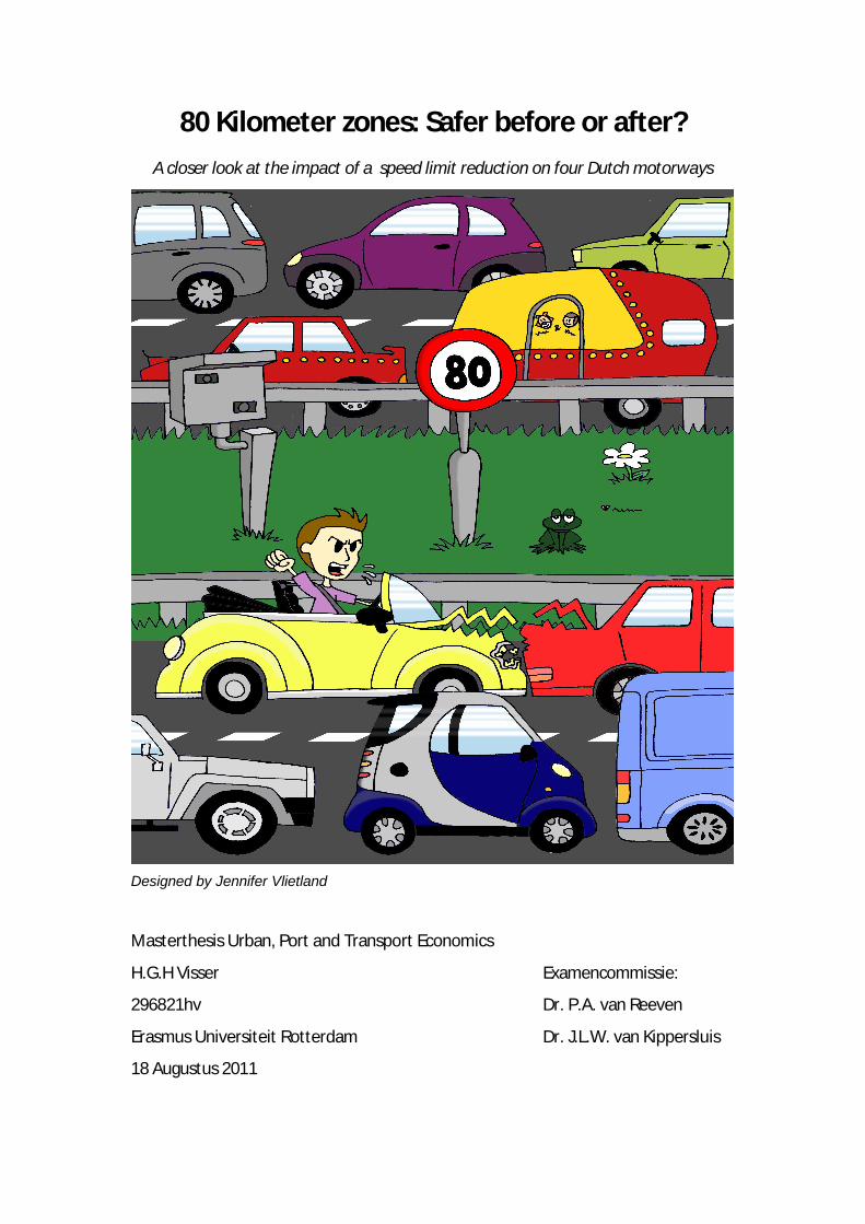
80 Kilometer zones: Safer before or after?

A closer look at the impact of a speed limit reduction on four Dutch motorways

Designed by Jennifer Vlietland

Masterthesis Urban, Port and Transport Economics

H.G.H Visser Examencommissie:

296821hv Dr. P.A. van Reeven

Erasmus Universiteit Rotterdam Dr. J.L.W. van Kippersluis

18 Augustus 2011

2

Abstract

This thesis discusses the combined impact of a reduction from 100 km/h to 80 km/h

and permanent speed enforcement on accidents, for four Dutch motorways. Chapter

1 introduces the main question: “What is the impact of the 80 kilometer zones policy

on road safety?” and is answered in Chapter 5. Current literature regarding speed,

road design and speed enforcement is reviewed and analysed in Chapter 2. The

chapter points out the added value of using control groups to correct for trends and

regression and two stage least squares analyses to improve statistical validity of the

results. Chapter 3 notes that Difference-in-Differences is rejected as a method due to

violation of permanent trends assumption and presents regression and two stage

least square analysis as valid tools to analyse the relationship between speed and

accidents. Chapter 4 presents the results from the regression and two stage least

square analysis. The reduction in speed limit reduced the speed and the amount of

accidents. An additional effect of enforcement was not found. As speed is a

significant factor affecting accidents, Chapter 5 concludes with the final outcome:

The introduction of the policy helped reducing speed and accidents and did not

cause any spill over effects. Increased speed enforcement help to improve traffic

flow, contrary to previous literature, camera’s itself did not affect accidents, only

speed. Future research could test if the observed results hold in general, irrespective

of road type and surrounding.

3

Executive Summary

Chapter 1 describes the 80 kilometer policy introduction and scope. The thesis

analyses the relationship between the introduction of the policy, speed and safety

and answers the main question: “What is the impact of the 80 kilometer zones policy

on road safety?”

Chapter 2 discusses the theoretical background and the current literature about

speed, design variables, speed enforcement and accidents. Decreased maximum

speeds yield between 0% and 50% less accidents. Traffic and design features like

ADT, lane width, road gradient and curvature have a significant effect on accidents

too, however, these factors are harder to adjust. Finally speed enforcement has a

positive net effect in the reduction of accidents between an average of 20 to 35

percent. This chapter concludes with noting the added value of using control groups

and two stage least squares analyses to overcome methodological issues.

Chapter 3 introduces the six hypotheses that are tested in Chapter 4. Next, the

selection of control groups, statistical methodology based on characteristics is

presented. Difference-in-Differences is rejected as a tool, due to violation of the

parallel trends assumption. Regression and two stage least squares analysis are

selected as statistical tools. Data is obtained from various sources and limitations like

availability, registration rate and regime are discussed. A detailed description of both

regression and two stage least squares, the assumptions and limitations is supplied

at the end of the chapter.

Chapter 4 presents the results from the regression and two stage least square

analysis. Due to symmetrical relationships between the dependent and independent

variables, instead of regression, two stage least square analyses, is used. A test for

the instruments of posted speed reduction and enforcements yields a significant

reduction in speed due to a lower limit and enforcement. Speed is tested significant

in reducing accidents, thus the policy proves effective and enhances safety on the

4

zones. Comparing adjacent motorways accidents to the national trend, no evidence

of spill over effects is found.

Chapter 5 answers the main question: “What is the impact of the 80 kilometer zones

policy on road safety?” The policy reduces the average speed, reducing accidents

and improving safety, without compromising network safety. Accident registration

improvement helps improving the validity of the found results. Furthermore another

study on more rural and different types of roads could reveal if the results found in

this thesis hold in general.

5

Preface / Voorwoord

For my grandmother, Willy Varwijk / Voor Oma, Willy Varwijk 7/2/1919 – 9/5/2011

Deze scriptie betekent het eind van een hoofdstuk en de start van een nieuw

hoofdstuk. Terugkijkend op mijn studie periode kan ik zeggen dat ik er zeer van

genoten heb; van start tot einde, van college tot scriptie. Ik heb ook dingen gedaan

die ik niet van mijzelf verwacht had: voorzitter worden van een studievereniging,

hoe je beeld door iets kan veranderen is enorm. Dit is ook iets wat een studie en

alles eromheen moet doen, je beeld veranderen, je breder maken en vooral jezelf

eens goed een spiegel voorhouden. Deze scriptie is een voorbeeld van die spiegel, hij

reflecteert wat jij in de afgelopen jaren bereikt hebt en hoe je dit invult, dit is ook

iets wat bij wetenschap hoort, de continue reflectie van bestaande regels,

procedures, aannames en vooral een kritische houding. Voor het tot stand komen

van deze scriptie was toch enige hulp nodig. Iedereen die heeft meegeholpen wil ik

hiervoor bedanken, maar een aantal mensen in het bijzonder. Vooral de mensen bij

de Dienst Verkeer en Scheepvaart wil ik bedanken voor hun opmerkingen, suggesties

en in het bijzonder wil ik Joris Kessels, en Henk Stoelhorst bedanken voor hun

begeleiding, antwoorden en kritische kanttekeningen. Verder zijn er een aantal

mensen, die op de achtergrond vooral morele steun hebben gegeven, ten eerste

mijn ouders en broer, die mijn humeur van tijd tot tijd verdragen hebben en mijn

vrienden, die ook hun tips en uitleg over stata (Remco bedankt!) hebben gegeven.

Ten slotte wil ik mijn begeleiders, Peran van Reeven en Hans van Kippersluis,

bedanken voor hun commentaar en hun kritische houding, waardoor ik een betere

beschrijving van mijn denkproces heb neergezet. Ze hebben ook van tijd tot tijd mij

de nodige hoofdpijn bezorgd met de nodige suggesties, maar ik heb ze met plezier

overgenomen. Het resultaat, daar ben ik trots op en hoop ik een bijdrage te leveren

in de discussie rondom snelheid en veiligheid op de Nederlandse wegen.

H.G.H. Visser

6

Table of contents

Page

Abstract 2

Executive Summary 3

Preface 5

Table of Contents 6

Chapter 1 Introduction 7

Chapter 2 Literature review 9

2.1 Changes in speed limits 9

2.2 Design features and speed enforcement 12

Chapter 3 Statistical methodology 14

3.1 Hypothesis and control group selection 14

3.2 Statistical test selection 17

3.3 Variable selection and data description 20

3.4 Selected methodology 23

Chapter 4 Results and outcomes 26

4.1 Regressions 26

4.2 Two stage least squares 29

4.3 Other results and observations 33

Chapter 5 Conclusion

5.1 Conclusions and reflection 34

5.2 Recommendations and final remarks 36

References 38

List of terms used 40

Appendix 41 - 44

7

Introduction

In November 2005 the Dutch national government instituted four motorway zones

with a lowered maximum speed limit from 100 to 80 km/h. A permanent speed

enforcement system was added to enforce the reduced speed. The four sections are

highlighted with a purple marking on the map.

Map 1: 80 kilometer zones highlighted in purple, created on National Geographics Maps Maker

Interactive at www.education.nationalgeographic.com/education/mapping/interactive-map

The aim of the lower speedlimit is to reduce the emissions and noise burden caused

by traffic. Additionally, the change in policy should not have a negative impact on

road safety and congestion. Rijkswaterstaat, the Dutch National Road Directorate,

concludes in a 2007 review that the amount of accidents was reduced significantly.

(Rijkswaterstaat, 2007) This improvement represents an external cost reduction

leading to economic savings.1 This analysis omits the impact of changing factors, spill

over effects and offers no explanation for the observed result. The use of control

1 Costs for an accident range from minor damage to the car and passenger, accidents leading to hospitalisation (€258.834) or even deadly accidents (€2.528.445) and costs due to time losses (ranging from €5,86 to €41,54 per hour). Source: SWOW, factsheet verkeersongevallen and KPVV, rekenen aan verkeershinder. Both available through their websites, no links due to changing locations.

8

groups to accounts for a trend in data and applying two stage least squares analyses

corrects for a symmetrical relationship between various variables. Finally, spill over

effects are analysed, to assess if no shifts of accidents to connected sections has

occurred.

The thesis focuses on the impact of the policy on safety and answers the following

research question: “What is the impact of the 80 kilometer zones policy on road

safety?” An integral approach to safety is applied and includes an analysis of spill

over effects. A simple regression is used to explore possible variables and a two

stage least square analysis is selected as the statistical method, as it is more robust

than regression and accounts for reversed causality between the dependant and

independent variable. The method tests which variable is significant and test if the

instrument used (Speed reduction) is significant. In the final two chapters, the results

are discussed using the current literature as a reference point and conclusions based

on the results are drawn.

The thesis contains 5 Chapters and starts with Chapter 1, this introduction. Chapter 2

describes the problem statement, scope and current literature. Chapter 2 concludes

with formulating the hypotheses which are tested in Chapter 4. Chapter 3 covers the

statistical methodology and starts with illustrating the chosen statistical method and

the assumptions which are tested later. Next a description of the data and the

characteristics is provided and the impact on the analysis is discussed. Chapter 4

discusses the results and reflects these using Chapter 2. Chapter 5 contains the

conclusions and policy recommendations for the policymaker. Finally, suggestions

and recommendations for further research are made.

9

Chapter 2 - Literature review

This chapter describes the current literature and discussion. The last section

illustrates why current methods do not reveal the true relationship between speed,

road design, enforcement and accidents.

2.1 Changes in speed limits

This section serves as the theoretical base, it discusses current literature and

provides the background of subject and analysis. The most recent research from

other scholars and institutions is used to examine the relationship between speed,

other factors and accidents.

The relationship between speed, design variables and other controllable factors is an

important topic reflected by literature. Speed is an important factor contributing to

accidents, it determines the probability of involvement and the severity of the

accident. (Aarts, 2004) The relationship between speed and accidents is not a 1-on-1

relationship, the actual speed is influenced by the human-vehicle-environment,

which is determined by the type of road and (design) characteristics, traffic variables,

incidents and other non observable variables (e.g. driver attitude, traffic

composition).2 Various scholars examine the relationship between speed and

accidents and the impact of a change in posted maximum speed limit, especially in

the USA, parts of Europe and Australia, the issue of safety and speed is well covered.

An overview of various studies and their results is described in table 1.

2 Suggestion for further reading: Feng (http://safety.fhwa.dot.gov/speedmgt/ref_mats/fhwasa09028/resources/TRR1779-SynthesisofStudies.pdf) and SWOV (2004) Snelheid, spreading in snelheid en de kans op verkeersongevallen, downloadable from the website, www.swov.nl

10

Table 1: Overview accident impact of speed changes

Author Country Change km/h

(Posted)

Change in

accidents

Methodology

Rijkswaterstaat

(1989)

NL + 20 km/h - 3 % Before and after study of

entire network

Farmer et al.

(1999)

USA + 16,1 km/h +15% to

17%

Before and after study, 12

groups, 18 control groups.

Peltola

(2001)

FIN - 20 km/h - 14% Before and after study,

only seasonal change.

Rijkswaterstaat

(2003)

appendix A

NL - 20 km/h

- 46% Before and after study,

period unclear.

Kloeden

(2004)

AUS - 10 km/h - 19,7% Before and after, treated

section with control

group (all other)

Elihu et al.

(2004)

IL +10 km/h +24% to

+50%

Before and after studies,

Woolley

(2005)

AUS

(states)

- 10 km/h 0 to

– 25,3%

Before and after, same

sections

Kockelman

(2006)

USA + 16,1 km/h + 3% Regression, 35 states, 10

changed speed.

Vejdirektoratet

(2008)

DEN + 20 km/h + 9% Before and after study.

Limited change on urban

motorways

Peltola (2001) studied a seasonal change in speed limit and found that a reduction in

accidents took place, whereas this could be a temporal change and a possible

increase during summer. Rijkswaterstaat (2003) reports a decrease of accidents on

the A13 motorway, though the before period covers a larger timeframe than the

after period, where in reality a stable or even an increase is the real outcome.

Woolley (2005) has different outcomes for different area’s, using only one variable in

11

a before and after study, making interpretation of the results difficult, this could be

explained by other non-observed factors. Woolley (2005) and Elihu et al (2004)

differentiate between urban and non-urban, and report different outcomes for each

level. This difference could be explained by non-observed variable (e.g. driver

behaviour) or traffic and design variables. Research from Farmer (1999) and

Kockelman (2006) in the USA has different outcomes, partially explained by different

selection of treated and control groups. This raises questions if the selection criteria,

included variables and techniques used are valid. Kockelman (2006) uses a

regression to explore the relationship between the amount of accidents and posted

speed limits and other static factors. This approach fails to incorporate the actual

speed, which is a better predictor and observes a change in behavior more

accurately. Furthermore regression does not address the different initial endowment

points and assumes that a linear relationship exists, whereas the real relationship

could be exponential. This approach does not correct for possible reversed causality

between variables, causing invalid results. Elihu et all. (2004) show a significant

increase after the raised speed limit in Israël, therefore raising questions if this is

peak in accidents is actually permanent or an outlier. Kloeden (2004) compares the

treatment roads with all other non-treated groups, where possible spill over effects

as suggested by Elihu et all (2004) are assumed zero, and could lead to faulty

conclusions. Finally an increase in speed, from 100 km/h to 120 km/h in The

Netherlands has lead, according to Rijkswaterstaat (1989) a reduction in accidents.

However, this reduction is relatively small and could be attributed to a longer time

trend, rather than policy. The Vejdirektoratet (2008) for example, notes a larger

increase, but only analyses a short period of time, omitting trends as well.

One notable observation, found throughout all studies is the actual change in speed

of the drivers, is marginally, ranging from 0.5 km/h to 7 km/h. This change reflects a

smaller impact on actual speed than expected based on the change in posted speed

limit. No explanation is offered for the phenomena in neither study, but indicates

that results can partially be attributed to the change in the speed limit.

12

2.2 Design features and speed enforcement

Speed is one factor influencing the amount of accidents; the road design, weather,

location and other characteristics are key factors in explaining accidents. Hadi et al.

(1995) examine this relationship using negative binomial Poisson regression for the

state of Florida. ADT, lane with, type of median, length and speed limits are noted as

significant, whereas median width didn’t prove significant. They note that length and

speed limits are positively significant, reducing the amount of accidents. This result

is not incorporating the actual speed and possibly explains why this relationship is

found. Milton and Mannering (1998) analyse data from the Washington

metropolitan area, using negative binominal poisson regression, and suggest that

section length, gradient, ADT, traffic composition, road width and curves (design)

have a significant influence on the amount of accidents. This result is reproduced by

Kockelman (2005), linear regression as well, for 30 other states and confirms these

factors for other locations within the USA. Milton and Mannering, Kockelman and

Hadi et al. only tested design factors however, (human) factors such as: actual speed,

homogeneity of traffic and other non-observed factors haven’t been tested but

affect speed and (in)directly, the amount of accidents. Therefore, these methods

might cause over dispersion towards the applied variables, omitting important

predictor variables and could suffer from distortions in data like trends. Both forms

of regressions do not account for initial endowment and assume a general constant

factor.

Furtermore, the introduction of permanent speed enforcement system

(trajectcontrole) could have a separate, additional or combined effect as well.

Literature regarding speed enforcement is vast, Wilson et al. (2011) conducted a

review of existing literature and concluded the following: All 28 studies found a

lower number of crashes in the speed camera areas after implementation of the

program. In the vicinity of camera sites, the reductions ranged from 8% to 49% for all

crashes, with reductions for most studies in the 14% to 25% range. (…) The studies of

longer duration showed that these positive trends were either maintained or

improved with time. (..) A reduction in the proportion of speeding vehicles (drivers)

13

over the accepted posted speed limit, ranged from 8% to 70% with most countries

reporting reductions in the 10 to 35% range. Speed camera’s are suggested to be an

instrument to reduce accidents and speed, questions arise if enforcement itself

could cause a reduction in accidents, as the effect of the speed reduction could be

more significant. Furthermore most of these studies are conducted on different

types of roads than urban highways, which have other features and factors

influencing accidents and safety, causing different outcomes across the board.

Contrary to Rijkswaterstaat (1989), Farmer (1998), Kockelman (2006),

Vejdirektoratet (2008), this thesis uses control groups to account for trends in data.

The inclusion of control groups also allows to test if the policy (instrument) had a

significant effect on safety. Contrary to all studies, this thesis uses the V85 speed

which represents the speed which is respected by 85 percent of the drivers, as this

reveals the real change in speed, rather than reduced limit. Usage of the real speed

provides a more realistic image of how speed and other variables affect accidents.

Regresssion is used by Kockelman (2006) to analyse the relationship between various

variables and their impact accidents. Regression assumes that no causal relationship

exists between exploratory variables, suspicion arises that some variables do

interact. Using two stage least squares analyses corrects for these interaction

effects, by the use of instruments. The change in speed limits and speed

enforcement are instruments which this thesis uses to correct interaction effects.

None of the previous research investigate the possibility of spill over effects, as

suggested by Elihu, to adjacent sections, whereas safety as a whole should not

decline due changes in speed on the 80 kilometer sections. The accident count on all

adjacent roads are plotted and compared to the national trend to investigate if these

effects occur. Finally, the author has suspicion that weather and economic variables

to influence speed and accidents and are included in the tests. Weather affects

speed, therefore is included in the two stage least squares. Economic variables could

reveal increased demand for transportation and a reduction in speed due to

congestion.

14

Chapter 3 - Statistical Analysis

Based on the previously discussed literature, hypotheses are formulated to help

answering the main question. A description of the selection process for the

preferred testing method is given and continues with presenting the data which is

used to run the test. In the final section, a detailed description of the statistical tests

is given.

3.1 Hypotheses and control group selection

This thesis aims to answer the following main question: “What is the impact of the

80 kilometer zones policy on road safety?” To provide a comprehensible answer, 6

hypotheses, based on the literature, are formulated and tested:

H1: The introduction of 80 kilometer show a significant reduction in the

85th percentile speed.

H2: Road- design and characteristics are significant predictors for the

amount of accidents.

H3: Other variables (e.g. GDP and weather) show a significant relationship

with accidents.

H4: The implementation of the 80 kilometer zones shows a significant

effect on accidents.

H5: The implementation of permanent traffic speed monitoring has a

significant effect on safety.

H6: Spill over effects occur.

These hypotheses are tested using variables obtained from various data sources.

First, the national trend is presented to understand the setting and assist in further

analysis. Figure 1, on the next page illustrates the national trend for the Netherlands

from 2004 to 2009 is shown. The total amount shows a steady decline and did so

during the last decade.3

3 See CBS and DVS statistics on the next page.

15

First, the decline can be attributed to increased safety measures, but in section 3.3 it

is illustrated that more factors contribute to this decline. Second, note especially

minor injuries and first aid accidents show the strongest decline. Finally, the severe

accidents (deadly, hospitalized) do not show a decline and accidents with

hospitalized victims’ shows a small increase relative to all other accidents.

Figure 1: National accident count – The Netherlands, source: DVS, CBS

This trend in data causes overestimation in the results obtained by before and after

studies like Peltola (2001), Rijkswaterstaat (2003), Elihu et al. (2004), Woolley (2005),

Vejdirektoratet (2008) and regression like Kockelman (2006). Using control groups

accounts for this pitfall and provides results adjusted for trends in data. Selection of

control groups is based on criteria noted in Chapter 2 and include human factors,

traffic and design variables. Expert opinions from the staff of DVS confirmed4 these

factors based on previous research and noted that ADT, amount of lanes, ramps,

location are determinants on the outcomes. For human factors, traffic and design

4 The experts where consulted separately and each was asked which criteria they suggest to select control groups

16

variables, the Randstad area and the city ring of Brabant5 form the pool of possible

control groups. Traffic composition is an important factor and is taken into

consideration as well. Based on the selection criteria, expert opinions from DVS, a

the final selection is presented below on map 2. A detailed overview is provided in

Appendix B.

Map 2: 80 zones and different control groups

Red: 80 zones Green: Groups without enforcement Purple: Enforcement zones

5 The Randstad area is roughly the provinces of North and South Holland, Utrecht and part of Gelderland. The city ring of Brabant is the area between Breda and Eindhoven.

17

3.2 Statistical test selection

The policy introduction can be described as a natural experiment where treatment is

given (speed reduction in conjunction with permanent speed enforcement) and

compare the result to a control group, which did not receive the treatment. The

Difference-in-Differences estimator is a tool to assess the impact of a policy, a drug

or any other ‘treatment’ given to a group or groups, hence it could be a tool to

statistically test our hypotheses. However, it only uses one dependent variable and

does not incorporate independent variables. Examples of DiD usage include; changes

in competition Hastings (2004) and policy by Meyer (1995). Figure 2 illustrates the

method graphically. The DiD is calculated by a special form of regression analysis and

controls for differences in levels between treatment and control groups6. DiD

assumes parallel trends through time for both the treatment and control group and

a constant treatment effect is assumed.

Figure 2: DiD graphical representation. DiD Estimator is AC

6 More about the DiD estimator, see appendix E

18

First, a test for the assumptions of the DiD estimator is performed. The treatment is

constant, the 80 kilometer zones where kept at the designated speed at all times. To

test the trend assumption, an overview of the amount of accidents for the 80

kilometer zones is illustrated in graph 3.. Next, the developments in all control

groups are illustrated in graph 4 and 5. Due to the timing of the policy, all data has

been adjusted to reflect the implementation.7 The graphs illustrate a much more

diverse development through time than initially expected. Some sections show a

decline through time, the 80 kilometer zones, A2 Eindhoven, A9 Amstelveen and the

A16 Rotterdam. Others show a more erratic development or remain nearly flat. A

parallel trend cannot be extrapolated from these observations, violating one of the

assumptions of the DiD analysis, making outcomes invalid. Based on the previous,

other statistical tests like regression and two stage least squares are more suitable to

use.

Figure 3: 80 kilometerzones, group 1 to 4. Appendix B illustrates which number

belongs to which road section. Legenda is in ascending order.

7 The 80 speed limit started on the 1st of November 2005. Therefore the count for 2005 starts at the 1st of November 2004 till the 31st of October 2005 and so on.

19

Figure 4 and 5: Accident count on control groups

20

3.3 Variable selection and data description

Based on conclusions from Chapter 2 design, traffic and other variables are selected.

Design variables include ramps, length8, curvature, median width and gradient.

Second, other variables could be ADT, average speed and speed violators.

Furthermore the economic variable GDP is added as a variable, to capture the

increased demand and increased congestion as a result. Finally weather related

variables are considered for the models, based on the influence of weather on actual

driven speed. Traffic and design variables, based on the data availability, are ADT

(INT), average speed (VGmid), length, and ramps. To test if the weather has a

significant influence on speed and on accidents, we test various variables like days of

rain (RAD), the total amount of rain (RTA), average duration of rain (RDU)and the

intensity of rain during a rainy day (RAI). Furthermore we add economic variables

like the Gross Domestic product (lnGDP), gasoline (diesel) and fuel prices (euro),

which could explain the impact of the costs of driving and increased congestion on

speed and accidents. Speed enforcement is noted as Contr. and is a binary variable.

Each variable and source is illustrated and the limitations of the data presented, we

start with the response variable and continue with the exploratory variables and

conclude with data transformation.

The accident data is supplied by the Data ICT Dienst (DID) of Rijkswaterstaat, part of

the Ministry of Infrastructure and Milieu. The data is collected by the Dutch police

based on the Proces Verbaal (PV)9 or minutes of the accident registration done by

the attending officers. The information from the PV is digitalised, loaded into a

central database for accident registration and is available to the DID/DVS. The

database contains information about the accident, the time, the location, the

severity and the amount of casualties. The dataset however, has limitations. The

following apply:

8 Only length and ramps are used as variables, data on other variables was not available. 9 The Proces Verbaal is the police document which describes the aspects of the accident, for example, the persons involved, the cars involved, the damage, the casualties, the severity of the injury and a recap of the accident.

21

- A police PV is needed for an accident to be an ‘official one’, hence accidents

without a PV go unregistered.

- Human error could lead to a faulty classification and incomplete data. Incomplete

data has been removed and represented < 10% of data for an entire motorway.

Accidents from 100 outside the selected groups are added as well, due to a possible

error of the noting the wrong hectometer, as the spot where the accident happened.

- Not all deadly accidents are registered as such. For example, if someone drives into

a tree and dies (suicide), this is not an official death count. Neither is a murder, this is

excluded as well.

- Driving under influence of alcohol or drugs, as stipulated by article 8 of the Dutch

Traffic Law and causing an accident is kept separate.

- The reported accidents (deadly, hospitalised) versus the actual accidents are

showing a steady decline. For deadly accidents, the reduction is modest, in 2001,

91% of total amount was reported, down to 84% in 2010, this is illustrated in figure

6. For hospitalised, in 2001, 69% was reported, down to 49% in 200910. For less

serious incidents, these numbers are unknown. For minor injuries and material

damage only, the registration rate is expected to be even lower.11

78%

80%

82%

84%

86%

88%

90%

92%

94%

96%

1996 1997 1998 1999 2000 2001 2002 2003 2004 2005 2006 2007 2008 2009 2010

Figure 6: Registration rate of deadly accidents, presented by M. de Wit and P. Mak;

accident registration 20 juni 2011. Based on COGNOS database.

10 Source: SWOV COGNOS database 11 Due to the nature of the accidents, they mostly do not require police assistance and can be dealt with by the involved persons and their insurance company’s. In 2009, nearly 2 million damage reports where filed by the insurance companies in 2009 and less than 10000 are officially reported by the police.

22

A final and separate note, road works impact the day to day operation of a

motorway, causing possible crashes and affecting speed. The author investigated this

variable in the dataset, but did not find a relationship between road works and

accidents, therefore it is excluded as a variable.

Traffic data like the ADT and Speed is monitored for locations if road loops are

present, or for ADT, a manual count is executed and is recorded by the DID. The

average speed is based on the V8512 of September and May13, excluding seasonal

effects. Weather related data is sourced from the KNMI14, based on the closest

observation location to the motorway. Finally, the GDP and fuel/gasoline prices are

sourced from the CBS. GDP is recorded yearly, fuel prices monthly.

First the data15 is transformed into yearly statistics, with a year being the 1st of

November of last year the virtual start and the 31st of October of the designated year

the last date, reflecting the policy implementation. The transformation to yearly

variables is based on the limited amount of accidents per month and improves

robustness. All accidents (regardless of type) are counted as one, splitting the

accidents into typologies and analyse each separately would be impossible due to

low rate of each separate group. Finally the complete set has been transferred to a

STATA database and prepared for statistical testing.

12 The V85, a variable that represents the speed that 85 percent of the drivers do not pass. 13 If only one month was available, this is used as the average. Individual differences between months where less than 0.2 km/h. 14 KNMI = The Royal Dutch Meteorological Institute, comparable to the English MET office. 15 GDP is the only exception to this rule.

23

3.4 Selected methodology

This section further illustrates the statistical tests and assumptions, starting with

regression and continuing with a two stage least squares analyses. The results are

reported in Chapter 3. and conclusions and recommendations based on the

outcomes are reported in Chapter 4.

We need to establish if the relationship between our variables is valid and assess

how they interact with each other, to test this, we run a regression analysis16.

Regression is a powerful tool to explore the relationship between one dependant

variable (response variable, Y) and multiple independent (exploratory variables

U1..Ui) with a respective coefficient β and an error term ε. A general regression

equation is described as:

ii UU *..* 11 with i = 1 .. v

Regression analysis assumes:

- A linear relationship

- Use of relevant (independent) variables

- Independent variables cannot be highly correlated, this leads to multicollinearity

and inaccurate estimators of the coefficient β.

- No heteroscedasticity of the error term; the error term is constant and should not

show a particular pattern. This could otherwise lead to insignificant variables to

become significant leading to false conclusions. In an optimal situation, the error

term is close to 0.

Regression assumes all variables are exogenous and are explained outside the

model, except the response variable Y which is endogenous. As noted earlier, speed

and accidents have reversed causality, hence making speed and endogenous variable

and explained within the model. The introduction of an instrument (or policy) allows

16 The description in the thesis covers the basics about regression. A (very) detailed description is obtainable at: http://www.law.uchicago.edu/files/files/20.Sykes_.Regression.pdf

24

to predict the endogenous variable, accounting for the reversed causality and

includes the effect of non observed variables on the variable S. The relationship is

illustrated in figure 7.

Figure 7: relation between speed (S), the amount of accidents (Y), the instrument (Z)

and a non observed variable (I)

Z

S Y

I

A two stage least squares regression solves the endogenous relationship by using an

instrument(s).17 In the first stage, U1 is regressed and the instrument (τ) tested. The

results from the first stage, the predicted values for U1 are used in the second stage

together with the other variables to create a regression with Y1 as a the response

variable and produces the respective coefficient (β) for each variable. The process is

illustrated below:

The initial regression:

iii UX *..* 11

with i = 1 .. v

Is split up into two stages:

iii UÛ *..* 111

iii UiYU **..* 111

with i = 1 .. v

17 The instrument has to be correlated with the variable of interest for reasons that can be verified an explained. And the instrument has to be uncorrelated with the outcome beyond the variable of interest. For the motorways, the introduction of the 80 kilometer maximum speed combined with permanent speed camera’s is our instrument

25

This is a cross sectional analysis which assumes independent results. We use the

same road sections in the panel, hence the observations are dependent. As a

correction, we add a time coefficient to the two stage least square function.

Furthermore the initial endowment point of each road section is different. To

account for this difference, we assume fixed effects. These fixed effects are constant

through time and reduces the unobserved variable bias.

After these changes, the relation becomes:

itititit UÛi *..* 11

ititiitit UiYU **..*11

with i = 1 .. v and t = 2002 … 2009

Due to the fixed effects assumption, the constant, i , is excluded, furthermore time

invariant variables are assumed to be part of the fixed effects. The assumptions for

the two stage, least square analysis are similar to regression:

- A linear relationship

- No heteroscedasticity of the error term; the error term should be constant

throughout and not show a particular pattern. This could otherwise lead to

insignificant variables to become significant leading to false conclusions. In an

optimal situation, the error term is close to 0.

- Endogenity of the variables; only applies to cross sectional two stage least square

analysis.

- A valid instrument or instruments need to be applied to correct for the symmetrical

relationship.

The instrument also determines if the outcomes are valid, as weak instruments do

not fully correct the symmetry, leading to ambiguous results. Furthermore, the

methodology does not account for underlying mechanisms and overestimation is a

risk. Finally, the results cannot be extrapolated into a general rule of thumb, due to

the changes in the underlying relationships.

26

Chapter 4 – Results and outcomes

This chapter presents the results of the various statistical methods and reflects

them. First, the outcomes from the regression are presented and analysed. Second,

the two stage least square outcomes are presented and interpreted. Finally, we

check if there is any evidence for spill over effects.

4.1 Regressions

First a regression of all selection variables is run, the results are shown in table 2.

Next the correlation is estimated and based on this pre-assessment, variables are

excluded from further research. A variable is tested using the t-stastic for

significance. We use an alpha of 5 percent, a variable is significant if the power is

smaller or equal to 0.05. Note that the amount of observations is limited due to data

availability, conclusions should be reviewed, taking this into account.

Table 2: Regression using all variables

_cons 819.0859 558.3714 1.47 0.150 -306.2376 1944.41 RTA .9988949 .6916927 1.44 0.156 -.3951201 2.39291 RDU 1.073997 1.234308 0.87 0.389 -1.413587 3.561582 RAD -.4581113 .2022823 -2.26 0.029 -.8657845 -.050438 RAI .1037627 .0592249 1.75 0.087 -.0155973 .2231227 ramps 6.78263 1.193382 5.68 0.000 4.377527 9.187733 length -2.099357 1.55315 -1.35 0.183 -5.229526 1.030812 VGmid_02 .2707368 .1703597 1.59 0.119 -.0726007 .6140743 lnGDP -60.42423 45.25503 -1.34 0.189 -151.6298 30.78129 diesel .9547177 .3999525 2.39 0.021 .1486663 1.760769 euro -.8934899 .5919175 -1.51 0.138 -2.086421 .2994414 lnINT 3.05725 7.865862 0.39 0.699 -12.79535 18.90985 TAC Coef. Std. Err. t P>|t| [95% Conf. Interval]

Total 10721.9286 55 194.944156 Root MSE = 9.2932 Adj R-squared = 0.5570 Residual 3799.99211 44 86.3634571 R-squared = 0.6456 Model 6921.93646 11 629.266951 Prob > F = 0.0000 F( 11, 44) = 7.29 Source SS df MS Number of obs = 56

27

Table 3: Correlation between the different variables.

VGmid_02 1.0000 VGmid_02

VGmid_02 -0.0738 -0.2717 -0.2557 0.1915 -0.3795 -0.0317 -0.1457 0.0394 -0.1312 -0.2727 -0.3674 lnINT -0.0979 0.0115 0.0135 -0.7633 -0.2968 -0.0934 0.0769 -0.0888 0.0022 0.0277 1.0000 lnGDP -0.3813 0.9033 0.8581 0.0000 -0.0000 -0.0540 0.1378 -0.0155 0.2233 1.0000 RAD -0.1130 0.4111 0.4820 0.0655 0.0829 0.0251 0.7491 0.7895 1.0000 RDU -0.0074 0.0299 0.1078 0.1469 0.0552 -0.1281 0.6645 1.0000 RTA -0.0315 0.2788 0.2882 -0.0146 0.0585 -0.0743 1.0000 RAI 0.2772 0.0777 0.0511 0.2330 0.2561 1.0000 ramps 0.6107 -0.0000 0.0000 0.5672 1.0000 length 0.2480 -0.0000 0.0000 1.0000 diesel -0.2910 0.9765 1.0000 euro -0.3361 1.0000 TAC 1.0000 TAC euro diesel length ramps RAI RTA RDU RAD lnGDP lnINT

Table 2 on the previous page illustrates a regression of the dependent variable TAC,

the Total Accident Count and other variables like INT, euro, diesel, lnINT, lnGDP,

VGmid RTA, RAD, RDU and RAI. It shows only ramps, diesel and RAD are significant at

the five percent level. Speed is not a significant variable, but notably RAD is the only

weather significant variable, whereas others are near significant. Other variables like

length, RDU, INT show high levels of insignificance. These findings can be influenced

by interaction effects. We use correlation to see if these effects occur and regress

again with non-interacting variables. A variable has perfect positive (1), or negative (-

1) correlation with respect to another, or no correlation at all (0). Any number

between is the degree to which variable A and B interact with each other. Table 3

illustrates the correlation coefficients, euro, diesel and GDP show strong signs of

correlation with each other. First of all, the prices of fuel are linked to each other, as

both are refined oil products. Their strong correlation with the GDP also makes

sense, as oil prices tend to follow the economic trend. Based on this logic, we

remove the diesel and euro variable due to their mutual correlation and the

correlation with the GDP. Weather variables like RAD, RDU and RTA show signs of

strong correlation too (>0.6), which can be explained by their nature. If it rains, a

certain amount drops in a certain timeframe, as it seems, for a longer period of time,

there is a shared average.

28

Table 4: Regression of selected variables, corrected for multicollinarity

_cons 398.6155 193.0775 2.06 0.043 13.53461 783.6963 RAI .0679932 .0543274 1.25 0.215 -.0403595 .1763458 ramps 5.829512 .9440097 6.18 0.000 3.946744 7.71228 length -.4475584 1.162266 -0.39 0.701 -2.765624 1.870507 VGmid_02 .1591793 .1220044 1.30 0.196 -.0841508 .4025094 lnGDP -35.69745 13.49173 -2.65 0.010 -62.60585 -8.789054 lnINT 5.51928 5.785699 0.95 0.343 -6.019932 17.05849 TAC Coef. Std. Err. t P>|t| [95% Conf. Interval]

Total 13854.8052 76 182.300068 Root MSE = 9.6368 Adj R-squared = 0.4906 Residual 6500.6956 70 92.8670801 R-squared = 0.5308 Model 7354.10959 6 1225.68493 Prob > F = 0.0000 F( 6, 70) = 13.20 Source SS df MS Number of obs = 77

In table 4, the outcome of a regression, using the uncorrelated variables is

presented. Ramps, lnGDP are the only significant factors, VGmid, RAI and lnINT

insignificant and length by an even larger margin. Ramps are significant and have a

negative impact on safety, this is reflected by observations in the dataset, accidents

tend to happen where users interact. These interactions happen at ramps, junctions

and other merging and seperation area’s. The natural logarithm of the GDP has a

negative impact, thus when GDP increases, a decline in accidents follows, this could

point toward an advancing safety in cars.18 Length is insignificant contrary to

expectations, whereas a longer section of road is expected to have more accidents.

The ADT does not offer any additional power as well, where we would expect it an

increase of traffic to increase the chance of getting into an accidents, due to more

interaction moments. Finally, speed is not signficant, in contradiction to what is

expected from literature. Hence, there could be other confounding factors, or a

relationship between the response variable and exploratory variable. Speed is

influenced not only by the driver, but also by weather, accidents and other drivers.

To account for this relationship, we start by using a two stage least square analyses

in Section 4.2 and discuss the outcomes.

18 E.g. improved sensors for distance, airbags and construction advancement.

29

4.2 Two stage Least squares

Table 5: (cross sectional) two stage least squares analysis outcomes

Instruments: RAI lnGDP lnINT length ramps Speedmax ContrInstrumented: VGmid_02 _cons 409.2887 189.3982 2.16 0.031 38.07515 780.5023 ramps 5.720198 1.008269 5.67 0.000 3.744026 7.696369 length -.3098123 1.247342 -0.25 0.804 -2.754557 2.134933 lnINT 5.645754 5.542801 1.02 0.308 -5.217937 16.50944 lnGDP -36.50308 13.29494 -2.75 0.006 -62.56068 -10.44548 RAI .0673575 .0518797 1.30 0.194 -.0343249 .1690398 VGmid_02 .1360396 .1509031 0.90 0.367 -.1597251 .4318042 TAC Coef. Std. Err. z P>|z| [95% Conf. Interval]

Root MSE = 9.1906 R-squared = 0.5306 Prob > chi2 = 0.0000 Wald chi2(6) = 86.01Instrumental variables (2SLS) regression Number of obs = 77

_cons 465.4411 124.9622 3.72 0.000 216.1482 714.7339 Contr 9.118493 1.935945 4.71 0.000 5.256389 12.9806 Speedmax .7744654 .077909 9.94 0.000 .6190411 .9298897 ramps -2.625383 .5240586 -5.01 0.000 -3.670852 -1.579915 length 2.230648 .6832886 3.26 0.002 .8675246 3.593772 lnINT .2173981 3.685553 0.06 0.953 -7.13508 7.569876 lnGDP -35.14078 8.960636 -3.92 0.000 -53.01676 -17.2648 RAI -.0016839 .0343984 -0.05 0.961 -.0703068 .066939 VGmid_02 Coef. Std. Err. t P>|t| [95% Conf. Interval]

Root MSE = 6.0548 Adj R-squared = 0.8322 R-squared = 0.8476 Prob > F = 0.0000 F( 7, 69) = 54.83 Number of obs = 77

From table 5 note that our instruments, the introduction of a reduced speed limit

(Speedmax, the instrument) and permanent speed enforcement (Contr) are

significant in the first stage, making them strong instruments which correct the

relationship between the various variables. During the second stage ramps is

significant as a predictor for accidents. The cross sectional analysis does not account

for the dependency of the various observations, as the observations are the same

motorway sections during different years. A Woolridge test with a value of 0.1209

confirms autocorrelation between the error term and a variable, based on this test,

lnINT is removed as it is correlated to the GDP. The Xtivreg command in stata allows

the program to recognise this dependency. The results from this adjustment, using a

panel based two stage least square analysis is noted in table 6.

30

Tabel 6: (panel) Two stage least squares accounting for dependency, results

Instruments: RAI lnGDP Contr SpeedmaxInstrumented: VGmid_02 F test that all u_i=0: F(11,76) = 13.65 Prob > F = 0.0000 rho .97027832 (fraction of variance due to u_i) sigma_e 7.8972541 sigma_u 45.121922 _cons -624.2691 226.594 -2.76 0.006 -1068.385 -180.153 Contr -.1707192 3.263224 -0.05 0.958 -6.566521 6.225083 lnGDP 28.45887 14.91242 1.91 0.056 -.7689261 57.68667 RAI .0322379 .0369315 0.87 0.383 -.0401466 .1046223 VGmid_02 2.764066 .4723671 5.85 0.000 1.838244 3.689889 TAC Coef. Std. Err. z P>|z| [95% Conf. Interval]

corr(u_i, Xb) = -0.9544 Prob > chi2 = 0.0000 Wald chi2(4) = 450.24

overall = 0.0032 max = 8 between = 0.0392 avg = 7.7R-sq: within = 0.3304 Obs per group: min = 7

Group variable: Group Number of groups = 12Fixed-effects (within) IV regression Number of obs = 92

F test that all u_i=0: F(11, 76) = 66.76 Prob > F = 0.0000 rho .94003221 (fraction of variance due to u_i) sigma_e 2.5221689 sigma_u 9.9858841 _cons 287.6727 50.7179 5.67 0.000 186.6593 388.6862 Speedmax .5435289 .0819975 6.63 0.000 .3802169 .706841 Contr 2.268083 1.186853 1.91 0.060 -.0957396 4.631907 lnGDP -18.84583 3.800421 -4.96 0.000 -26.41502 -11.27663 RAI -.0075314 .0118773 -0.63 0.528 -.0311871 .0161242 VGmid_02 Coef. Std. Err. t P>|t| [95% Conf. Interval]

corr(u_i, Xb) = 0.4861 Prob > F = 0.0000 F(4,76) = 27.00

overall = 0.6652 max = 8 between = 0.6984 avg = 7.7R-sq: within = 0.5870 Obs per group: min = 7

Group variable: Group Number of groups = 12Fixed-effects (within) regression Number of obs = 92

In the first stage, the instrument Speedmax is significant and reduces the actual

speed. This confirms the observed reductions in Chapter 2. Speed camera’s do not

reduce speed as much as a posted reduction, they enforce the maximum and help to

limit extremes and do not have an additional effect on accidents when the posted

limit is lowered, as observed in the second stage. To fully verify this, an additional

instrument needs to be added, testing a speed reduction, without additional speed

enforcement, on motorways for the Netherlands. The author examined this option,

but concluded that suitable sections and data for this test are lacking. Contrary to

earlier studies about speed camera, the camera itself does not reduce accidents, it

does however, lower speed and thus accidents. GDP decreases speed, due to

increased demand for mobility as GDP rises, leads to increased congestion.

31

Figure 8: Speed development on two 80 zones.

6065707580859095

2002 2003 2004 2005 2006 2007 2008 2009

Year

Spee

d in

km

/h

A20 RTMA10 AMS

The implementation of the zones reduced the speed on average, by 10 km/h.

Comparing this with previous literature, in which reductions ranging from 0.5 to 7

km/h where realised, this reduction is higher. As speed camera’s smoothing traffic

and, as illustrated in the first stage, increase speed, this difference. Based on these

results hypothesis 1 (H1) is not rejected, as the policy reduced the 85th percentile

speed, figure 8 illustrates this reduction after implementation of the policy in 2005.

During the second stage, the predicted speed is used and regressed with all variables

on the total amount of accidents. First, ramps and length are omitted, as illustrated

in Appendix D, this because we use a fixed effects model and as they remain

constant over time, they are excluded from this analysis. Based on regression, we do

argue that they do contribute to amount of accidents, but due to model

assumptions, cannot be further tested. Hypothesis 2 is therefore not rejected, due to

the outcomes of regression. Second, RAI and lnGDP are not significant, VGmid is

significant, assuming a alpha of 5 percent. The weather, according to this analysis,

has no influence on the amount of accidents. An explanation for this phenomena is

adjusted driver behaviour, which anticipate better and allow larger margins. GDP is

significant in reducing speed, but does not lower accidents by itself, which could be

explained by the increased road usage. Therefore Hypothesis 3 is rejected.

Speed is significant with a p-value of 0.000 and (a rounded) coefficient of 3. Based

on the literature discussed in Chapter 2, the result confirms earlier findings about

32

the relation between speed, a reduction and the related amount of accidents.

Suspicion arises that the factor 3 is overestimated, when compared to the coefficient

of the regression and literature. This overestimation might be caused by the limited

amount of observations, combined with the range (between 68 km/h and 123 km/h)

in which these observations are. Even if overestimated, a reduction maximum

allowed speed helps to reduce the amount of accidents on the motorway when

compared with various control groups. The overall safety therefore benefits from a

reduction in speed. This confirms hypothesis 4, as the introduction of the 80

kilometer zones reduced the speed by 10 km/h, as this reduced the amount of

accidents. Hypothesis five is rejected, as permanent enforcement has no effect on

speed and thus accidents.

The results need to viewed into the current setting. All groups represent roads with

high levels of ADT, short sections, many ramps, motorway features and often urban

surroundings. The amount of observations is limited, this could cause a bias, or

overestimation, for example, speed as a factor. The underlying mechanisms of the

system are not incorporated into the two stage least square analysis and cannot be

extrapolated. The analysis does reveal the important factors and points towards an

overall positive effect on safety by the implementing a reduced speed on the

selected motorways.

This thesis takes an integral approach to safety for network, the next section checks

if no spill over effects occur on adjacent motorways.

33

4.3 Other results and observations

As suggested by Elihu et al. (2004), spill over effects could occur on adjacent road

sections of the 80 kilometer zones, reducing overall network safety. This shift in

accidents could be caused by changes in behavior and traffic. In figure 8, a plot of the

accident count on all adjacent sections to the 80 kilometer zones is displayed. The

decline of accidents, in accordance with the trend illustrated in figure 1 on page 14,

is observed. After the implementation of the zones in 2005, no increase in accidents

is noted, neither a weaker decrease. Though one could argue that the decrease in

2008 is a lagged reaction, this is unlikely due to the immediate correction

afterwards. More likely, this is a peak, the same kind of peak measured in 2003 but

overall, the declining trend as depicted in figure 1 is still observed. The graph shows

no evidence for a partial or a permanent spill over effect, hence hypothesis 6 is

rejected. The changes implemented on the 80 kilometer zones have no negative

impact on adjacent motorways and the safety of the motorway network as a whole,

maintained.

Figure 9: Accidents on the spill over zones

Spill over zones

0

50

100

150

200

250

2002 2003 2004 2005 2006 2007 2008 2009

Year

Acc

iden

t Co

unt

Spill over zones

34

Chapter 5 - Conclusions and recommendations

5.1 Conclusions and reflection

The implementation of the 80 kilometer zones on four motorways has external

effects, accidents is of them. The (negative) external costs associated with accidents

are costs incurred by the general public and translate to an economic loss. This thesis

investigates the relationship between the introduction of the policy, speed and

safety and answers the main question: “What is the impact of the 80 kilometer zones

policy on road safety?” To provide an answer on the main question, the following six

hypotheses are formed and tested:

H1: The introduction of 80 kilometer show a significant reduction in the

85th percentile speed.

H2: Road- design and characteristics are significant predictors for the

amount of accidents.

H3: Other variables (e.g. GDP and weather) show a significant relationship

with accidents.

H4: The implementation of the 80 kilometer zones shows a significant

effect on accidents.

H5: The implementation of permanent traffic speed monitoring has a

significant effect on safety.

H6: Spill over effects occur.

Hypothesis 1 is not rejected, based on the two stage least square analysis from

Chapter 4, which reveals that the implementation of the policy reduced the speed

significantly. This confirms earlier results from literature discussed in Chapter 2.

Hypothesis 2 is not rejected, based on the regressions from Chapter 3. Due to

assumptions for the two stage least square analysis, no further evidence could be

found to reject this hypothesis. ADT has been removed due to interaction with GDP

as the GDP explains an increase in traffic. Hypothesis 3 is rejected, based on analysis

from Chapter 3 as neither proved significant in reducing accidents. GDP however

35

does reduce speed, therefore a partial effect is observed. Hypothesis 4 is not

rejected, as the two stage least square analysis reveals that the zone policy is

effective in lowering speed and speed a significant factor for accidents, hence the

policy reduced the amount of accidents. However, the exact magnitude seems

overestimated, when comparing the literature from Chapter 2 and the regression

analysis. Still, a significant reduction can be attributed to this policy change.

Hypothesis 5 is rejected, contrary to outcomes as reported by Wilson (2011) from

various studies regarding speed camera’s and accidents. The enforcement is a

weaker instrument than a speed reduction, as it does not alter the limit, only

enforces it. This implies that a camera does reduce speed, but the camera itself does

not directly reduce accidents. Hypothesis 6 is rejected, no evidence of short, or long

term spill over effects could be found when comparing them to the trend illustrated

in figure 1. The increased safety on the treated motorway section, did not affect

adjacent sections negatively. The results need to be viewed in light of the restrictions

of the data and chosen methodology. However, the analysis reveals important

factors and points towards an overall positive effect on safety by the implementing a

reduced speed on the selected motorways.

Now, the main question posed in the introduction is answered: “What is the impact

of the 80 kilometer zones policy on road safety?” The implementation of the policy

reduced the speed on the zones and through the statistical test, revealed that this

speed reduction had a significant negative effect on the amount accidents. The

observed lower speed can be attributed to a reduction in maximum speed.

Additional effects from permanent enforcement where limited, as they have a

stronger effect on speed, rather than accident. The policy implementation did not

cause a shift of accidents to other adjacent sections of motorway, the safety of the

network as a whole did not deteriorate and increased on the 80 kilometer zones.

36

5.2 Recommendations and final remarks

The following recommendations are split between the Netherlands and

recommendations in general.

For the Netherlands:

- Improved registration of all accidents, including accidents that incur the Dutch

article 8 violations, the ‘driver suicides into a tree’ accidents and in general a more

precise tracking of the persons involved. Better registration provides a more detailed

insight into the actual amount of casualties that eventually die as a result of the

accident. This also provides more reliable data, which allows better policy and

accident analysis.

- In general, road data is available, but sometimes not logged enough (weather data)

or selectively available (speed data), which makes pre-selection of study objects

difficult and limits validity. The choice the policymaker needs to make is if this is

worth the effort.

- Analyse if a speed reduction without permanent enforcement proves as effective as

the 80 kilometer zones. This also provides a better understanding how the speed

choice is influenced, either by posted speed, enforced speed or accepted speed

relating to the road.

- Policymakers need to assess how the balance between time savings, costs and

safety is made. Investments in road safety could lead to long term benefits and

should not only be judged by short term costs.

In general:

- An integral approach to safety should be aspired. Analyse if spill over effects occur,

the suggestion from Elihu has been reviewed in this thesis and refuted, however, it

could hold in other countries and locations due to changing environments.

- If a researcher conducts this type of investigation for his/her country, provide an

English summary as well, it makes comparing results easier, reduces any translation

errors and provides a better understanding of safety related research, policies and

their impact.

37

- Include the registration rate of accidents in your analysis of safety, as a reduction in

accidents could be attributed to a decrease in registration quality instead of policy.

- Future research should focus on which adjustment (in design, speed or other

measures) proves most effective in reducing accidents. This allows policymakers to

make better assessments on which field they want to invest or improve.

- Additional research towards the change in driver behavior, linked towards the

different scenarios. This helps to understand the different attitudes and why

behavior changes after policy implementation.

- Another study could test if the observed results hold in general, or if other factors

contribute to a different. By using rural motorways and roads as groups, comparing

results with this thesis, such results could prove important for making policy

decisions about speed and safety.

Finally the author would like to express his gratitude for the cooperation from

Rijkswaterstaat in supplying him with the necessary data and background

information to perform this analysis, without this cooperation, this thesis would not

be realized.

38

References:

Athey and Imbens (2005) Identification and Inference in Nonlinear Difference-In-

Differences Models, NBER 2005

Alex et al. (2007) Propensity score and difference-in-difference methods: a study of

second-generation antidepressant use in patients with bipolar disorder, Health

Services and Outcomes Research Methodology, Health Services and Outcomes

Research Methodology, Volume 7, numbers 2-3 and 23-38.

Aarts, L.T. (2004) Snelheid, spreiding in snelheid en de kans op verkeersongevallen,

Stichting Wetenschappelijk Onderzoek Verkeersveiligeheid, Leidschendam

Buckley, J & Shang, Y (2003) Estimating Policy and program effects with

observational data: the differences-indifferences estimator. Practical Asessment,

Research & Evaluation, 8(24). http://pareonline.net/getvn.asp?v=8*n=24

Haji, A et al. (1995) Estimating safety effects of cross-section design for various

highway types using negative binomial regression, Transporation research board,

record 1500

Hastings, J (2004) Vertical Relationships and Competition in Retail Gasoline Markets”,

by Justine Hastings, American Economic Review, 2004

Kloeden, CN, Hutchinson, TP, McLean, AJ, Long, AD (2006) Reduction of speed limit

from 110 km/h to 100 km/h on certain roads in South Australia: a preliminary

evaluation, Centre for Automotive Safety Research, University of Adelaide

Kockelman, K (2006) Safety impacts and other implications of raised speed limits on

High-Speed roads, Transportation Research Board of the National Academies

Kockelman, K (2005) The safety effects of speed limit changes: use of Panel models,

including speed, use and design variables. To be Presented at the 84th Annual

Meeting of Transportation Research Board

Meyer, B. D., Viscusi, W. K. and Durbin, D. L. (1995), Worker's Compensation and

Injury. Duration: Evidence from a Natural Experiment", American Economic Review,

85, 322-340.

39

Milton, J and Mannering, F (1998) The relationship among highway geometrics,

traffic-related elements and motor-vehicle accident frequencies, Transportation

(1986-1998): Nov 1998; 25,4; ABI/INFORM global

NHTSA (1997) Traffic Safety Facts 1996: Speeding. US Department of Transportation,

6pp

Nilson, G (2004) Traffic safety dimensions and the Power Model to describe the effect

ofs peed on safety. Bulletin 221. Lund Institute of Technology.

Peltola, H (2000) Seasonally changing speed limits. Effects on speed and accidents.

Transportation Research Record, 1734, 46-51

Richter et al. (2004) Raised Speed limits, Speed Spillover, Case-Fatality Rates and

Road Deaths in Israel: A 5-Year Follow-Up, American Journal of Public Health, April

2004, Vol 94, No. 4

Rijkswaterstaat (1989) Evaluatie snelheidslimieten, 1 jaar na invoering van een nieuw

limietenstelsel op autosnelwegen. Rotterdam november 1989, ministerie van Verkeer

en Waterstaat

Rijkswaterstaat (2003) Evaluatie 80 km/uur-maatregel A13 Overschie, Ministerie van

Verkeer en waterstaat

Rijkswaterstaat (2007) Evaluatie 80 kilometerzones, eindrapportage. Ministerie van

Verkeer en Waterstaat. Page 5-8, 21, 23, 24

The Institute of Transport Economics (2004) Speed and Road Accidents, an

evaluation of the power model. Page IV – V

Volz, BD (2009) downloadable from: http://www.econ.uconn.edu/working/2009-

32.pdf

Wilson C, Willis C, Hendrikz JK, Le Brocque R, Bellamy N (2011) Speed cameras for

the prevention of road traffic injuries and death, published in the Cochrane Library,

issue 2

Woolley, J (2005) Recent advantages of lower speed limits in Australia, Journal of

Eastern Asia Society for Transportation Studies, Vol 6 pp. 3562 – 3573

40

List of terms used:

ADT: Average Daily Traffic

CBS: Centraal Bureau voor de Statistiek

DiD: Difference-in-Differences

DID: Data ICT Dienst

DVS: Dienst Verkeer en Scheepvaart

GDP: Gross domestic Product

INT: short for the Dutch intensiteiten, translates to ADT

KNMI: Koninklijk Nederlands Meteorologisch Institutuut

PV: Process Verbaal

RWS: Rijkswaterstaat

RAI: Rain Average Intensity, proxy for the average rain per shower, yearly

RAD: Rain Amout of Days, amount of days of rain per year

RDU: Rain Duration, the average during of a rain shower per year

RTA: Rain Total Amount, the total amount of rain per year

SWOV: Stichting Wetenschappelijk Onderzoek Verkeersveiligheid

VGmid: Average speed per year on the motorways.

V85: The speed which 85th percent of the drivers do not cross.

Zone: Instrument, implementation of a speed reduction from 100 km/h to 80 km/h

41

Appendix A - Results A13 Motorway study Rijkswaterstaat.

Table from Rijkswaterstaat (2003) p. 27. This table illustrates the Ammount of

Accidents (Aantal ongevallen) and Ammount of Victims (Aantal slachtoffers) before

(voor) and after (na) the implementation of the of the policy.

42

Appendix B – Treatment, control and enforcement groups

A2 = Motorway

- X en X = Between section X and section X, (..) group – max speed.

* = 80 kilometer zones, reduction from 100 km/h to 80 km/h

^ = speed enforcement zones

A2 - Knooppunt Oudenrijn en Everdingen (5) – 100 km/h - Knooppunt Vught en Knooppunt Hintham (6) --120 km/h - Knooppunt Batadorp en de Hogt (7) – 100 km/h A4 - Hoofddorp en Nieuw Vennep (17)^ - 120 km/h A9 - Knooppunt Badhoevedorp en Holendrecht (8) – 100 km/h A10 - de Coentunnel en Knooppunt de Nieuwe Meer* (1) - Knooppunt Coenplein tot de Zeeburgertunnel (14) – 100 km/h A12 - Voorburg en Den Haag* (2) - Knooppunt Oudenrijn en Knooppunt Lunetten, alleen de paralelbanen* (3) - Afslag Zoetermeer Centrum tot Knooppunt Prins Clausplein (9) – 120 km/h - Afslag De Meern en afslag Woerden (18)^ - 120 km/h - Knooppunt Velperbroek en Knooppunt Waterberg (15)^ - 100 km/h A13 - Tussen afrit Berkel en Rodenrijs en Knooppunt Kleinpolderplein (16)^ - 80 km/h A16 - Drechttunnel en afslag ’s-Gravendeel (10) – 100 km/h - Afslag IJsselmonde en afslag Kralingen (11)v- 100 km/h A20 - Knooppunt Kleinpolderplein en Crooswijk* (4) - Knooppunt Terbregseplein en afslag Nieuwekerk aan den IJssel (12) – 120 km/h A28 - Knooppunt Rijnsweerd en Den Dolder (13) – 100 km/h

43

Appendix C - DiD estimator

TABLE 1 Before After Increase

Treatment group α α + γ γ

Control group α + β α + γ + β + δ γ + δ

Difference β δ + β δ (DiD estimate)

Mathematically the model is the following:

1) Treatment effect is constant over time

ii ,0,1

2) For the use of a regression model we note the following equation

iiiiii tTtT )(

3) If we include more covariates into the model, the equation becomes

iiiiiii XtTtT ...)( 19

The coefficients and variables have the following interpretation for the 80 kilometer

zones:

i = The amount of accidents at time i .

= Constant term over time

= Treatment group specific effect20

iT = Treatment group is 1, or 0 otherwise

= Time trend common to control and treated groups

it = Time, 1 for t = 1 and 0 for otherwise

= True effect of treatment

iX = Other observed variables (e.g. average speed)

= Effect of other variables

ε = Error term for each unit at each time period

19 There is also an option to extend the model even more with time and group specific covariates, see Buckley & Shang (2003) 20 Accounts for average permanent differences between the treatment group and the control group.

44

Appendix D – Stata output, Fixed effects

Instruments: RAI lnGDP Contr length ramps SpeedmaxInstrumented: VGmid_02 F test that all u_i=0: F(11,76) = 6.50 Prob > F = 0.0000 rho .97027832 (fraction of variance due to u_i) sigma_e 7.8972541 sigma_u 45.121922 _cons -624.2691 226.594 -2.76 0.006 -1068.385 -180.153 ramps (omitted) length (omitted) Contr -.1707192 3.263224 -0.05 0.958 -6.566521 6.225083 lnGDP 28.45887 14.91242 1.91 0.056 -.7689261 57.68667 RAI .0322379 .0369315 0.87 0.383 -.0401466 .1046223 VGmid_02 2.764066 .4723671 5.85 0.000 1.838244 3.689889 TAC Coef. Std. Err. z P>|z| [95% Conf. Interval]

corr(u_i, Xb) = -0.9544 Prob > chi2 = 0.0000 Wald chi2(4) = 450.24

overall = 0.0032 max = 8 between = 0.0392 avg = 7.7R-sq: within = 0.3304 Obs per group: min = 7

Group variable: Group Number of groups = 12Fixed-effects (within) IV regression Number of obs = 92

F test that all u_i=0: F(11, 76) = 38.11 Prob > F = 0.0000 rho .94003221 (fraction of variance due to u_i) sigma_e 2.5221689 sigma_u 9.9858841 _cons 287.6727 50.7179 5.67 0.000 186.6593 388.6862 Speedmax .5435289 .0819975 6.63 0.000 .3802169 .706841 ramps (omitted) length (omitted) Contr 2.268083 1.186853 1.91 0.060 -.0957396 4.631907 lnGDP -18.84583 3.800421 -4.96 0.000 -26.41502 -11.27663 RAI -.0075314 .0118773 -0.63 0.528 -.0311871 .0161242 VGmid_02 Coef. Std. Err. t P>|t| [95% Conf. Interval]

corr(u_i, Xb) = 0.4861 Prob > F = 0.0000 F(4,76) = 27.00

overall = 0.6652 max = 8 between = 0.6984 avg = 7.7R-sq: within = 0.5870 Obs per group: min = 7

Group variable: Group Number of groups = 12Fixed-effects (within) regression Number of obs = 92