Embed Size (px)
Citation preview

Applied Reactor Technology and Nuclear Safety Chapter 8
8. Thermal-Hydraulic Analysis of Two-Phase Flows in Heated Channels
This section is dealing with the thermal-hydraulic analysis of two-phase flows in heated channels. Figure 8.0.1 shows the various two-phase flow patterns encountered over the length of a heated channel, together with the corresponding heat transfer regions.
Fluidtempe-rature
Subcooledboiling
Slugflow
Mistflow
AnnularFlow withentrainment
Annularflow
Bubblyflow
Single phaseliquid flow
Single phasevapor flow
Flow pattern Heat transfer regions
Convective heattransfer to liquid
Saturatednucleate boiling
Forcedconvective heattransfer throughliquid film
Dryout
Post-dryoutheat transfer
Convective heattransfer to vapor
x=1
x=0
Temperature
Walltemperature
Figure 8.0.1. Flow patterns and regions of heat transfer in convective boiling.
_____________________________________________________________________ Henryk Anglart Rev. 0 Page 8-1

Applied Reactor Technology and Nuclear Safety Chapter 8
Several of the heat transfer regions shown in Fig. 8.0.1 are encountered in fuel assemblies of LWRs. During normal operation of a nuclear power plant the following regions are present: convective heat transfer to liquid, subcooled boiling, saturated nucleate boiling and forced convective heat transfer through liquid film. During abnormal operation two other regions can occur: post-dryout heat transfer and convective heat transfer to vapor. Details of the various heat transfer regimes will be given in the following sections. In addition, two types of Critical Heat Flux (CHF) will be discussed in some detail.
8.1 Onset of Nucleate Boiling In Chapter 7 it has been shown that the coolant temperature in a channel heated with a uniform heat flux is a linear function of the distance from the inlet as follows,
GAczPqTzT
p
Hfif
′′+=)( . (8.1.1)
The saturated nucleate boiling starts at z = zsc, where the bulk liquid temperature Tf(z) equals Ts, the saturation temperature. The length of the subcooled region zsc can be readily obtained from Eq. (8.1.1) as,
( ) subiH
pfis
H
psc T
PqGAc
TTPqGAc
z ∆′′
=−′′
= , (8.1.2)
where is the so-called inlet subcooling. subiT∆ Assume that the subcooled boiling start at z = znb (znb is the length of non-boiling region). In the single-phase region, when 0 < z < znb, the clad surface temperature TC and the liquid bulk temperature Tf are related to each other as follows,
hqTTT ffC ′′=∆≡− , (8.1.3) where h is the heat transfer coefficient to single phase liquid under forced convection and
is the temperature difference between the surface of the heated wall and the bulk liquid.
fT∆
_____________________________________________________________________ Henryk Anglart Rev. 0 Page 8-2
Applied Reactor Technology and Nuclear Safety Chapter 8
Wall temp Tw
Bulk liquid temp Tl
zsc
zfdb
znb
supT∆
subT∆
G
Saturation temp
Figure 8.1.1. Wall and liquid temperature distribution in subcooled boiling. Combining Eq. (8.1.1) and (8.1.3) yields the following expression for the clad surface temperature,
+′′+=
′′+=
hGAczPqT
hqzTzT
p
HfifC
1)()( . (8.1.4)
It is convenient to introduce a so-called wall superheat defined as a difference of the temperature of the heated wall surface and the saturation temperature. The wall-superheat can be obtained from Eq. (8.1.4) as,
+′′+∆−=−≡∆
hGAczPqTTzTzT
p
HsubisC
1)()(sup (8.1.5)
It is clear that no boiling will occur when 0sup <∆T , since the wall temperature is below the saturation temperature. However, there is no clear and easy criterion to define such wall superheat at which the subcooloed boiling will start. This quantity has been investigated by many researches. Bergles and Roshenow proposed the following correlation for the Onset of Nucleate Boiling (ONB),
( )( 0234.016.2sup
156.1 8.11083 pONB Tpq ∆⋅⋅=′′ ) , (8.1.6)
_____________________________________________________________________ Henryk Anglart Rev. 0 Page 8-3
Applied Reactor Technology and Nuclear Safety Chapter 8
where is the heat flux at onset-of-nucleate-boiling [W mONBq ′′ -2], p is pressure [bar] and is wall superheat [K]. supT∆
Another model was proposed by Davies and Anderson, who proposed the following analytical solution,
2sup)(8
TT
Hq
gfs
fgffgONB ∆
−=′′
ρρσλρρ
. (8.1.7)
Here σ is the surface tension [N m-1], is the latent heat [J kgfgH -1] and fλ is the liquid conductivity [W K-1 m-1]. Combining Eqs. (8.1.6) or (8.1.7) with (8.1.5) yields the distance znb at which the subcooled boiling starts. Bowring proposed another approach, based on an arbitrary assumption that the non-boiling length znb, or the onset-of-nucleate-boiling point is located where the wall temperature calculated from single-phase convective heat transfer would be equal to the wall temperature calculated from the subcooled boiling heat transfer, that is ( ) ( )SCBCSPLC TT = , (8.1.8) or
( )nsf qThqzT ′′⋅+=′′
+ ψ)( . (8.1.9)
Bowring’s expression for the local subcooling for the onset of nucleate boiling is thus as follows
( )nONBsub qhqzT ′′⋅−′′
=∆ ψ)( (8.1.10)
The right-hand-side of Eq. (8.1.9) is a general form of a correlation for wall temperature in subcooled boiling heat transfer. Several such correlations have been published in the literature. One example is the Jens and Lotes correlation, developed for subcooled boiling of water flowing upwards in vertical electrically heated stainless steel or nickel tubes. The correlation for the wall temperature is as follows
62/25.0
61025 p
sC eqTT −
′′
+= (8.1.11)
It should be noted that this correlation is valid for water only and that it is dimensional: T is in [K], q’’ is in [W m-2] and p is absolute pressure in [bar].
_____________________________________________________________________ Henryk Anglart Rev. 0 Page 8-4

Applied Reactor Technology and Nuclear Safety Chapter 8
More recently, Thom et al. reported that the wall superheat obtained from (8.1.11) was consistently under-predicted in comparison with their measurements. They proposed the following modified correlation
87/5.0
61065.22 p
sC eqTT −
′′
+= , (8.1.12)
and all variables are dimensional in a similar manner as in the Jens-Lotes correlation.
8.2 Subcooled and Saturated Flow Boiling Subcooled boiling region is divided into two sub-regions: partial subcooled boiling and fully-developed subcooled boiling region. In the partial subcooled boiling region only few nucleation sites are active and a considerable portion of the heat is transferred by normal single-phase forced convection. When the wall temperature increases, the number of active sites also increases and the area for single-phase heat transfer decreases. As the wall temperature is increased further, the whole surface is covered by active nucleation sites and boiling starts to be fully-developed. Bowring suggested the following heat flux partitioning in the partial boiling region,
scbspl qqq ′′+′′=′′ , (8.2.1) where is the total average surface heat flux, qq ′′ spl′′ is the average surface heat flux transferred by single-phase convection and qscb′′ is the average surface heat flux transferred by bubble nucleation. The single-phase convection part qspl′′ can be calculated in the same way as in single-phase region, e.g. by using Eqs. (7.1.1) with (7.1.3). For the bubbly-nucleation part qscb′′ Rohsenow proposed a correlation derived for nucleate pool boiling,
( ) rs
r
fgsf
pgffgfscb HC
TcgHq /
/1
sup5.0
Pr−
∆
−=′′
σρρ
µ , (8.2.2)
where r = 0.33 and s = 1.0 for water and 1.7 for other fluids. The constant Csf may vary from one fluid-surface combination to another. For water on mechanically polished stainless steel, the coefficient is equal to 0.0132. Experimental data indicate that there is a correlation between the heat flux at the onset of nucleate boiling and the heat flux at which boiling becomes fully developed. This correlation has been approximated by Forster and Grief as
_____________________________________________________________________ Henryk Anglart Rev. 0 Page 8-5
Applied Reactor Technology and Nuclear Safety Chapter 8
ONBFDB qq ′′=′′ 4.1 (8.2.3) This observation leads to the following expression for the local subcooling at the fully developed boiling location, due to Bowring,
n
FDBsubq
hqzT
⋅′′
−′′
=∆ 6104.14.1)( ψ (8.2.4)
Saturated flow boiling region occurs in fuel assemblies of BWRs where nearly complete vaporization of the coolant is desired. To avoid the high wall temperatures and/or the poor heat transfer associated with the saturated film-boiling regime, the vaporization must be accomplished at low superheat or low heat flux levels. When boiling is initiated, both nucleate boiling and liquid convection may be the active heat transfer mechanisms. The importance of the two mechanisms varies over the channel length. As vaporization occurs, void fraction rapidly increases causing flow acceleration and, as a result, an enhancement of the convective heat transfer. The increasing void fraction and acceleration of flow causes changes in the flow pattern along the boiling channel. For vertical upward flow, the flow pattern changes from bubbly to slug, churn and the annular flow. Correspondingly, the heat transfer regime changes from nucleate flow boiling to evaporation of the liquid film in annular flow. Further, it is clear that, as vaporization continues, the thickness of the liquid film will decrease, reducing its thermal resistance and thereby enhancing the effectiveness of this mechanism. When the liquid film becomes very thin, the required superheat to transport the wall heat across the liquid film become so low that nucleation is completely suppressed, and the only heat transfer mechanism is heat conduction through the liquid film. It should be clear that prediction of the convective boiling heat transfer coefficient requires an approach that accommodates a transition from a nucleate-pool-boiling-like condition at low qualities to a nearly pure film evaporation condition at higher qualities. One of the most popular correlations for prediction of heat transfer coefficient in saturated flow boiling is the Chen correlation. The fundamental assumption is that the total heat transfer coefficient is a superposition of two parts: a microscopic (nucleate boiling) contribution hmic and a macroscopic (bulk convective) contribution hmac:
macmic hhh += (8.2.5) The bulk-convective contribution is evaluated using the Dittus-Boelter equation,
FD
h fmac ⋅
= 4.08.0 PrRe023.0
λ. (8.2.6)
Here liquid Reynolds number is defined as,
_____________________________________________________________________ Henryk Anglart Rev. 0 Page 8-6

Applied Reactor Technology and Nuclear Safety Chapter 8
µDxG )1(Re −
= . (8.2.7)
S is the so-called suppression factor evaluated as,
( 117.1463.16 Re1056.21 −− ⋅⋅+= FS ) , (8.2.8) where F is found as,
≥
+
≤= −
−
1.01213.035.2
1.011
1
tttt
tt
XX
XF , (8.2.9)
and the Martinelli parameter is given by
1.05.09.01
−
=g
f
f
gtt x
xXµµ
ρρ
. (8.2.10)
The microscopic contribution (nucleate boiling) to the overall heat transfer coefficient is determined by applying a correction to the Forster-Zuber relation for the heat transfer coefficient for nucleate pool boiling,
( ) SpTpTH
ch fCs
gfgf
fpffmic ⋅−∆
= 75.024.0
sup24.024.029.05.0
49.045.079.0
)(00122.0ρµσ
ρλ . (8.2.11)
The Chen correlation has to be applied as follows: 1. Given mass flux, fluid properties, local heat flux and quality; guessed wall superheat 2. Find Xtt from Eq. (8.2.10) 3. Find Re from Eq. (8.2.7) 4. Find F from Eq. (8.2.9) 5. Find S from Eq. (8.2.8) 6. Find hmac from Eq. (8.2.6) 7. Find hmic from Eq. (8.2.11) 8. Find h from Eq. (8.2.5) 9. Find superheat as ∆ hqT /sup ′′=10. Repeat 7 through 9 until convergence is achieved
8.3 Occurrence of Critical Heat Flux The conditions at which the wall temperature rises and the heat transfer decreases sharply du to a change in the heat transfer mechanism are termed as the Critical Heat Flux (CHF) conditions. The nature of CHF, and thus the change of heat transfer mechanism, varies
_____________________________________________________________________ Henryk Anglart Rev. 0 Page 8-7
Applied Reactor Technology and Nuclear Safety Chapter 8
with the enthalpy of the flow. At subcooled conditions and low qualities this transition corresponds to a change in boiling mechanism from nucleate to film boiling. For this reason the CHF condition for these circumstances is usually referred to as the Departure from Nucleate Boiling (DNB). At saturated conditions, with moderate and high qualities, the flow pattern is almost invariably in an annular configuration (see Fig. 8.0.1). In these conditions the change of the heat transfer mechanism is associated with the evaporation and disappearance of the liquid film and the transition mechanism is termed as dryout. As indicated in Fig. 8.0.1 once dryout occurs, the flow pattern changes to the liquid-deficient region, with a mixture of vapor and entrained droplets. It is worth noting that due to high vapor velocity the heat transport from heated wall to vapor and droplets is quite efficient, and the associated increase of wall temperature is not as dramatic as in the case of DNB. The mechanisms responsible for the occurrence of CHF (DNB- and dryout-type) are not fully understood, even though a lot of effort has been devoted to this topic. Since no consistent theory of CHF is available, the predictions of CHF occurrence relay on correlations obtained from specific experimental data. LWR fuel vendors perform their own measurements of CHF in full-scale mock-ups of fuel assemblies. Based on the measured data, proprietary CHF correlations are developed. As a rule, such correlations are limited to the same geometry and the same working conditions as used in experiments. Most research on CHF published in the open literature has been performed for upward flow boiling of water in uniformly heated tubes. The overall experimental effort in obtaining CHF data is enormous. It is estimated that several hundred thousand CHF data points have been obtained in different labs around the world. More that 200 correlations have been developed in order to correlate the data. Discussion of all such correlations is not possible; however, some examples will be described in this section. One of the earliest correlations was given by Bowring, who proposed the following expression to evaluate the CHF condition:
( )zC
HHGDAq cifs
crit +−⋅+
=′′4/
, (8.3.1)
where
GDFHGDF
AB
B21
2
lg1
0143.01579.0+
⋅⋅= , (8.3.2)
( )( )pB
B
GFGDFC 00725.02
4
3
1356347.01077.0
−+⋅
= , (8.3.3)
_____________________________________________________________________ Henryk Anglart Rev. 0 Page 8-8
Applied Reactor Technology and Nuclear Safety Chapter 8
Here D is the hydraulic diameter in [m], G is the mass flux in [kg m-2 s-1], Hfg is the latent heat in [J kg-1], p is the pressure in [bar], Hfs is the enthalpy of saturated liquid at local pressure and Hci is the inlet enthalpy. The correlation parameters FB1, FB2, FB3 and FB4 are functions of pressure and are given in a graphical form (not shown here, but these who are interested can found the plots in Liquid-Vapor Phase Change Phenomena, Van P. Carey, Hemisphere 1992). The correlation is based on a fit to data in the ranges 136 < G < 18600 [kg m-2 s-1], 2 < p < 190 [bar], 2 < D < 45 [mm] and 0.15 < z < 3.7 [m]. For upflow boiling of water in vertical tubes with constant applied heat flux, Levitan and Lantsman recommended the following correlation for DNB in 8-mm-diameter pipe:
( )[ ]{ }x
xp
crit eGppq 5.198/9825.02.12
1000986.1
988.73.10 −
−−
+−=′′ . (8.3.4)
For dryout they recommended the following relation for predicting the critical quality for 8-mm pipe:
5.032
10009868.0
9804.2
9857.139.0
−
+
−+=
Gpppxcrit (8.3.5)
In these relations critq ′′ is in [MW m-2], p is the pressure in [bar], G is the mass flux in [kg m-2 s-1]. The correlation (8.3.4) is valid in ranges 29.4 < p < 196 [bar] and 750 < G < 5000 [kg m-2 s-1] and is accurate to ±15%. For correlation (8.3.5) the ranges are 9.8 < p < 166.6 [bar] and 750 < G < 3000 [kg m-2 s-1] and the accuracy of xcrit is ±0.05. Both these correlations can be used for CHF in tubes with other diameters by using proper correction factors. The CHF given by Eq. (8.3.4) can be used for other tube diameters if the following correction factor is applied:
5.0
8
8
⋅′′=′′
Dqq
mmcritcrit , (8.3.6)
where D is the tube diameter in [mm] and
mmcrit 8′′q is the critical heat flux obtained from
Eq. (8.3.4). In a similar manner, the critical quality given by Eq. (8.3.5) can be used for other tube diameters with the following correction factor:
15.0
8
8
⋅=
Dxx
mmcritcrit . (8.3.7)
_____________________________________________________________________ Henryk Anglart Rev. 0 Page 8-9
Applied Reactor Technology and Nuclear Safety Chapter 8
Here mmcritx
8 is the critical quality obtained from Eq. (8.3.5) and D is the tube diameter in
[mm].
8.4 Post-CHF Heat Transfer As indicated in Fig. 8.0.1, if the flow boiling process exceeds the dryout condition, the post-dryout heat transfer will occur. This situation is valid for high-quality flow boiling crisis and is termed as the post-dryout heat transfer or the mist flow evaporation. At low qualities and subcooled conditions the DNB may occur and will be followed by the convective film boiling at the heated walls. The film boiling is associated with sudden and very high wall temperature increase. A sustained film boiling at high mass flux levels causes wall temperatures so high that most conventional materials would melt. Due to that the DNB and the following film boiling must be avoided in fuel assemblies of LWRs. In addition, even experimental measurements of DNB and film boiling are quite difficult. Convective film boiling For convective film boiling at low to moderate rates the flow takes on the so-called inverted annular pattern. The vapor film is covering the heated wall and isolating water from the wall. The film is generally not smooth but exhibits irregularity at random locations. Several investigators have linked these distortions of the water-vapor interface to the growth of waves due to interface instability. For laminar conduction-dominant transport, the heat transfer coefficient through the vapor film is given by
δλgh = . (8.4.1)
Here δ is the vapor film thickness and gλ is the vapor conductivity. The vapor film thickness can be obtained from a simple one-dimensional model. Substituting the predicted film thickness to (8.4.1) yields,
( )( ) ( )
413
4
−−−
=satCgCHF
gfggfg
TTzzgH
hµ
λρρρ (8.4.2)
This simplified model, however, takes no account for the bubbles that rise with film and its accuracy is not very good. Another model based on Bromley’s equation for film boiling from horizontal cylinder and using the Helmholtz length scale is as follows,
_____________________________________________________________________ Henryk Anglart Rev. 0 Page 8-10
Applied Reactor Technology and Nuclear Safety Chapter 8
( )( )
4/13
62.0
−−
=HsatCg
fggfgg
TTgH
hλµ
ρρρλ, (8.4.3)
where Helmholtz-unstable wavelength is defined as,
( ) ( )
2/1
2355
534
24.16
−−=
satCggfg
gfgH TTg
Hλρρρµσ
λ (8.4.4)
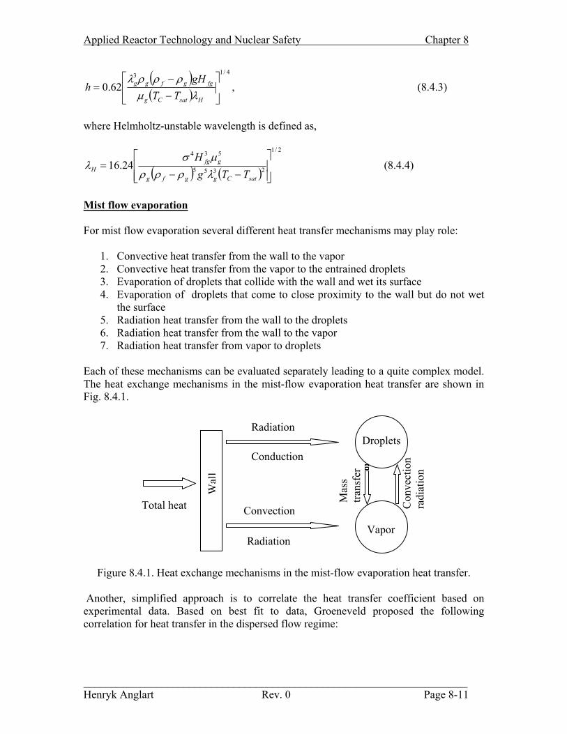
Mist flow evaporation For mist flow evaporation several different heat transfer mechanisms may play role:
1. Convective heat transfer from the wall to the vapor 2. Convective heat transfer from the vapor to the entrained droplets 3. Evaporation of droplets that collide with the wall and wet its surface 4. Evaporation of droplets that come to close proximity to the wall but do not wet
the surface 5. Radiation heat transfer from the wall to the droplets 6. Radiation heat transfer from the wall to the vapor 7. Radiation heat transfer from vapor to droplets
Each of these mechanisms can be evaluated separately leading to a quite complex model. The heat exchange mechanisms in the mist-flow evaporation heat transfer are shown in Fig. 8.4.1.
RadiationDroplets
Conduction
Con
vect
ion
radi
atio
n
Mas
s tra
nsfe
r
Wal
l
Total heat Convection
Vapor Radiation
Figure 8.4.1. Heat exchange mechanisms in the mist-flow evaporation heat transfer. Another, simplified approach is to correlate the heat transfer coefficient based on experimental data. Based on best fit to data, Groeneveld proposed the following correlation for heat transfer in the dispersed flow regime:
_____________________________________________________________________ Henryk Anglart Rev. 0 Page 8-11

Applied Reactor Technology and Nuclear Safety Chapter 8
( ) dcwg
b
f
g
gg
YxxGDahD,g Pr1Nu
−+
==
ρρ
µλ, (8.4.5)
where
( ) 4.0
4.0
111.01 xYg
f −
−−=
ρρ
. (8.4.6)
Note that Prg,w is the vapor Prandtl number evaluated at the wall temperature and all other parameters are evaluated at saturation temperature. Values of the constants a, b, c and d are provided for tubes and annuli only, see Table 8.4.1. Table 8.4.1 Coefficients in the Groeneveld’s correlation (8.4.4) Geometry a b c d Tubes 0.00109 0.989 1.41 -1.15 Annuli 0.0520 0.688 1.26 -1.06 Tubes and annuli 0.00327 0.901 1.32 -1.5 The validity of the correlation is limited to the following ranges: 2.5 < D < 25 mm, 68 < p < 215 bar, 700 < G < 5300 [kg m-2 s-1], 0.1 < x < 0.9, 120 < q’’ < 2100 kW m-2, 0.88 <
Prg,w < 2.21, 0.706 < Y < 0.976 and 6.6 104 < ( )
−+
xxGD
f
g
g
1ρρ
µ < 1.3 106.
8.5 Void Fraction Distribution in Boiling Channels When both the vapor and the liquid phase of coolant are flowing in a channel the flow is termed as two-phase flow. The fundamental feature that distinguishes two-phase flows from single-phase flows is the presence of an interface between the two phases. The shape and the motion of the interface is usually a part of the solution and is not known à priori. That makes a solution of two-phase flow problems much more difficult than the solution of single phase problems. The objective of this lecture is to present the basic features of two-phase flows in fuel assemblies of nuclear reactors. It will be shown how the basic parameters, like void fraction and pressure drop can be predicted. It will be assumed that two-phase mixture consists of a gas (or vapor) phase, always designed with the g subscript, and the liquid phase, designed with the l subscript. Static quality of the two-phase mixture is defined as a ratio of the vapor mass to the total mixture mass,
MM
MMM g
lg
g =+
=χ . (8.5.1)
_____________________________________________________________________ Henryk Anglart Rev. 0 Page 8-12

Applied Reactor Technology and Nuclear Safety Chapter 8
The volume of the vapor in the mixture divided by the total volume of the mixture is termed the void fraction. In analogy to Eq. (8.5.1), the volume-averaged void fraction is computed as,
VV
VVV g
lg
g =+
=α . (8.5.2)
The static quality can be expressed in terms of the volume-averaged void fraction (and vice-versa) using the following relationships: ggg VM ρ= and lll VM ρ= ,
−
+=
+=
+=
αα
ρρ
ρρρρ
ρχ
11
1
1
1
g
l
gg
llllgg
gg
VVVV
V, (8.5.3)
and
−+
=+
=+
=
χχ
ρρ
ρρρρ
ρα
11
1
1
1
l
g
gl
lgllgg
gg
MMMM
M. (8.5.4)
For flowing mixtures, these quantities can be computed in terms of the cross-sectional areas in the channel occupied by liquid, Al, and vapor, Ag. The cross-section averaged void fraction is thus given as,
lg
g
AAA+
=α . (8.5.5)
The mass flow rate is usually represented by symbol W and has unit [kg/s]. The individual mass flow rates of liquid and vapor will be Wl and Wg, respectively, and their sum will be equal to W. The mass flow rates of vapor and liquid can be expressed in terms of cross-section areas and phase velocities, ul and ug, as follows,
ggggllll AuWAuW ρρ == , . (8.5.6) In boiling channels it is convenient to use the fraction of the total mass flow which is composed of vapor and liquid. The mass flow quality is defined as,
WW
WWW
x g
lg
g =+
= . (8.5.7)
_____________________________________________________________________ Henryk Anglart Rev. 0 Page 8-13
Applied Reactor Technology and Nuclear Safety Chapter 8
In a similar manner as for the static quality, the flowing quality can be expressed in terms of the cross-section averaged void fraction as,
−⋅⋅+
=+
=+
=
αα
ρρ
ρρρρ
ρ11
1
1
1
g
l
g
l
ggg
llllllggg
ggg
uu
AuAuAuAu
Aux . (8.5.8)
The void fraction becomes,
( )( ) ( )
−⋅⋅+
=⋅⋅+
=+
=
xx
uu
uu
WWuWuW
uW
l
g
l
g
l
g
l
g
g
llllggg
ggg
11
1
1
1
ρρ
ρρρρ
ρα . (8.5.9)
8.5.1 Homogeneous Equilibrium Model In this model the phases are assumed to be in equilibrium – both in the mechanical and the thermodynamic sense. The mechanical equilibrium assumption means that both phases are well mixed and move with the same velocity. The thermodynamic equilibrium assumption means that both phases co-exist in the saturation form; none of them is in the superheated or subcooled condition. The energy balance for a two-phase mixture can be written as,
[ cchc dHzHWdzPqzHW ]+⋅=⋅⋅′′+⋅ )()( (8.5.1-1) which is very similar to the energy balance for the single-phase flow. The enthalpy distribution is thus obtained as,
[ ]W
Pqdz
zdHdHzHWdzPqzHW hc
cchc⋅′′
=⇒+⋅=⋅⋅′′+⋅)(
)()( (8.5.1-2)
For constant heat flux this yields,
zW
PqHzH hcic
⋅′′+=)( (8.5.1-3)
Eq. (8.5.7) defines so called mass flow quality. In addition, there is a definition of the mixture quality based on enthalpies,
fg
fH H
HHx
−≡ (8.5.1-4)
_____________________________________________________________________ Henryk Anglart Rev. 0 Page 8-14
Applied Reactor Technology and Nuclear Safety Chapter 8
For HEM the flow and the thermodynamic quality are equivalent, that is xH = x. Combining Eq. (8.5.1-3) and Eq. (8.5.1-4) yields,
zHWPqxzx
fg
hi ⋅
⋅′′+=)( (8.5.1-5)
The void fraction has been expressed as a function of local flow quality in Eq. (8.5.9). Since in the Homogeneous Equilibrium Model the phasic velocities are equal, e.g., Ug = Ul, (8.5.1-6) The expression for the void fraction reduces to,
−⋅+
=
xx
l
g 11
1
ρρ
α . (8.5.1-7)
Combining Eq. (8.5.1-7) with (8.5.1-5) gives the distribution of the void fraction as a function of the axial distance in a channel.
8.5.2 Drift Flux Model Presence of the vapor phase has a significant influence on the local value of the mean coolant density. This, in turn, influences the local neutron flux and thus the local power. Clearly, there is a feedback between the local power and the local void fraction. Due to that it is very important to be able to accurately estimate the local value of the void fraction. Eqs (8.5.4) and (8.5.9) give expressions for the void fraction in stationary and flowing mixture, respectively. In case of the stationary mixture Eq. (8.5.4) gives an exact expression for the void fraction. Knowing the densities of phases and the static quality, the corresponding void fraction can be computed. Example 8.5.2-1: Comparison between the static quality and the void fraction. A tank contains a mixture of air and water, with Ma = 1 kg and Mw = 999 kg. Calculate the void fraction of the mixture assuming aρ = 1 kg/m3 and wρ = 1000 kg/m3. Solution: The static quality is found as ( ) 001.099911 =+=χ and the void fraction as
( ) ( )( ) 50025.0001.01000999.0111 =⋅⋅+=α . Thus, it would seem that the mass fraction of air is negligible (only 0.1%), whereas the air fills more then half of the vessel (50.025%). This example illustrates the importance of considering both the void fraction and the quality.
_____________________________________________________________________ Henryk Anglart Rev. 0 Page 8-15
Applied Reactor Technology and Nuclear Safety Chapter 8
More interesting is the case with the flowing mixture, unfortunately, an accurate prediction of void fraction is much more complex. Apparently Eq. (8.5.9) can be used for that purpose; however, one has to know the slip ratio, S = ug / ul. This parameter is not constant and depends in a complex manner on flow quality x, pressure, mass flux and flow regime. Typically the slip ratio has been found from two-phase flow measurements. In the simplest case it can be assumed that the phases move with the same velocity and thus the slip ratio is equal to 1. This assumption is a fundamental part of the so-called Homogeneous Equilibrium Model (HEM). According to this model, void fraction can be found from Eq. (8.5.4) and is a function of local quality and pressure only. A direct and essential extension of the slip ratio approach is the Drift Flux Model (DFM) proposed by Zuber and Findlay (1965). The model enables the slip between the phases as well as it takes into account the spatial pattern of the flow. Given a two-phase mixture flowing in a pipe, the following local quantities can be defined:
( ) ll uj α−≡ 1 , (8.5.2-1)
gg uj α≡ , (8.5.2-2)
gl jjj += , (8.5.2-3) ( )( )lgggj uujuu −−=−≡ α1 , (8.5.2-4)
where α is the local void fraction and uk is the local velocity of phase k (k = g for the vapor phase and k = l for the liquid phase). From Eq. (8.5.2-4) one gets,
jjjuu gggj αααα −=−= . (8.5.2-5) Eq. (8.5.2-5) can be integrated over the channel cross-section to obtain,
dAjdAjdAuAA
gA gj ∫∫∫ −= αα , (8.5.2-6)
where A is the channel cross-section area. The following definitions can be introduced:
A
dAu
dA
dAuU A gj
A
A gjgj α
α
α
α ∫∫∫ =≡ , (8.5.2-7)
AJCdAjdACdAj
AAA
⋅⋅⋅=⋅≡ ∫∫∫ ααα 00 , (8.5.2-8)
∫=A
gg dAjA
J 1 . (8.5.2-9)
_____________________________________________________________________ Henryk Anglart Rev. 0 Page 8-16
Applied Reactor Technology and Nuclear Safety Chapter 8
Combining Eqs (8.5.2-6) through (8.5.2-9) yields,
gj
g
UJCJ+
=0
α . (8.5.2-10)
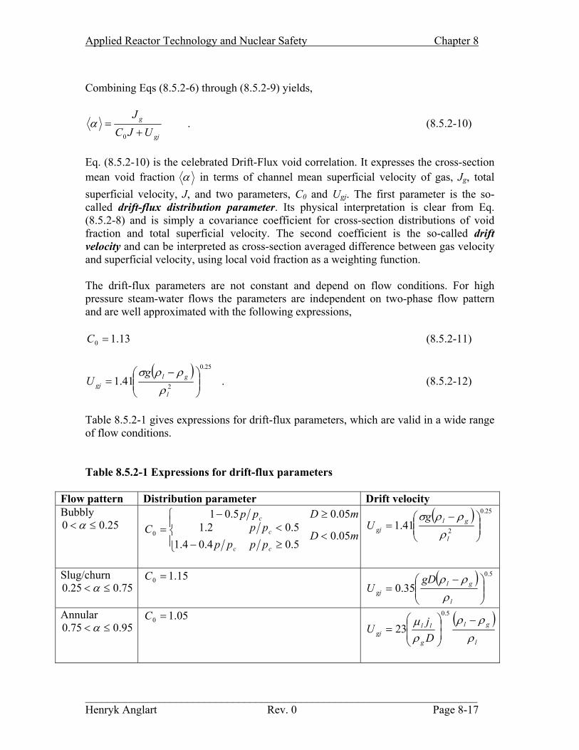
Eq. (8.5.2-10) is the celebrated Drift-Flux void correlation. It expresses the cross-section mean void fraction α in terms of channel mean superficial velocity of gas, Jg, total superficial velocity, J, and two parameters, C0 and Ugj. The first parameter is the so-called drift-flux distribution parameter. Its physical interpretation is clear from Eq. (8.5.2-8) and is simply a covariance coefficient for cross-section distributions of void fraction and total superficial velocity. The second coefficient is the so-called drift velocity and can be interpreted as cross-section averaged difference between gas velocity and superficial velocity, using local void fraction as a weighting function. The drift-flux parameters are not constant and depend on flow conditions. For high pressure steam-water flows the parameters are independent on two-phase flow pattern and are well approximated with the following expressions,
13.10 =C (8.5.2-11)
( ) 25.0
241.1
−=
l
glgj
gU
ρρρσ
. (8.5.2-12)
Table 8.5.2-1 gives expressions for drift-flux parameters, which are valid in a wide range of flow conditions. Table 8.5.2-1 Expressions for drift-flux parameters
Flow pattern Distribution parameter Drift velocity Bubbly
25.00 ≤< α
<≥−<
≥−= mD
pppppp
mDppC
cc
c
c
05.05.04.04.15.02.1
05.05.010
( ) 25.0
241.1
−=
l
glgj
gU
ρρρσ
Slug/churn 75.025.0 ≤< α
15.10 =C ( ) 5.0
35.0
−=
l
glgj
gDU
ρρρ
Annular 95.075.0 ≤< α
05.10 =C ( )l
gl
g
llgj D
jU
ρρρ
ρµ −
=
5.0
23
_____________________________________________________________________ Henryk Anglart Rev. 0 Page 8-17
Applied Reactor Technology and Nuclear Safety Chapter 8
Mist 195.0 << α
0.10 =C ( ) 25.0
253.1
−=
g
glgj
gU
ρρρσ
The drift-flux void correlation given by Eq. (8.5.2-10) can be expressed in terms of the quality and mass flux as follows,
GxU
xxC
GU
GG
CJU
JJJ
CUJC
J
gjg
l
g
g
gjg
g
l
l
g
g
gj
g
lggj
g
ρρρ
ρρρ
α
+
−+
=
+
+
=+
+=
+=
11
1
1
11
0
000
. (8.5.2-13)
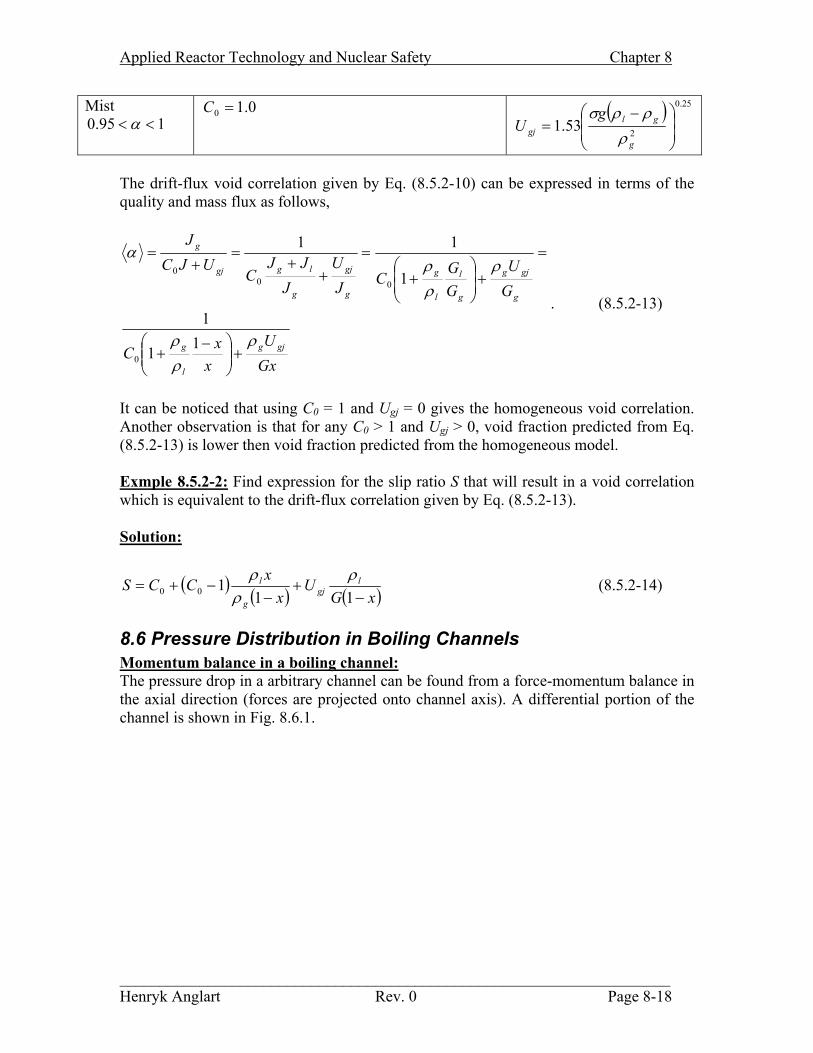
It can be noticed that using C0 = 1 and Ugj = 0 gives the homogeneous void correlation. Another observation is that for any C0 > 1 and Ugj > 0, void fraction predicted from Eq. (8.5.2-13) is lower then void fraction predicted from the homogeneous model. Exmple 8.5.2-2: Find expression for the slip ratio S that will result in a void correlation which is equivalent to the drift-flux correlation given by Eq. (8.5.2-13). Solution:
( ) ( ) ( )xGU
xx
CCS lgj
g
l
−+
−−+=
11100
ρρρ
(8.5.2-14)
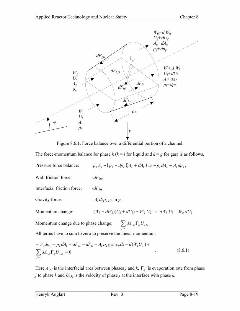
8.6 Pressure Distribution in Boiling Channels Momentum balance in a boiling channel: The pressure drop in a arbitrary channel can be found from a force-momentum balance in the axial direction (forces are projected onto channel axis). A differential portion of the channel is shown in Fig. 8.6.1.
_____________________________________________________________________ Henryk Anglart Rev. 0 Page 8-18
Applied Reactor Technology and Nuclear Safety Chapter 8
Wg+d WgUg+dUgAg+dAgpg+dpg
dAi,gl
dFgi
dFlw
WgUgAgpg
dFgw
WlUlAlpl
Wl+d WlUl+dUlAl+dAlpl+dpl
ϕ
dz
g
dFli
glΓ
Figure 8.6.1. Force balance over a differential portion of a channel.
The force-momentum balance for phase k (k = l for liquid and k = g for gas) is as follows, Pressure force balance: ( )( ) kkkkkkkkkk dpAdApdAAdppAp −−⇒++− , Wall friction force: -dFkw, Interfacial friction force: -dFki, Gravity force: - ϕρ singdzA kk , Momentum change: -(Wk + dWk)(Uk + dUk) + Wk Uk → -dWk Uk - Wk dUk Momentum change due to phase change: ∑
≠
Γkj
kjikjkji UdA ,,
All terms have to sum to zero to preserve the linear momentum,
0)(sin
,, =Γ
+−−−−−−
∑≠
kjikj
kjkji
kkkkkikwkkkk
UdAUWddzgAdFdFdApdpA ϕρ
. (8.6.1)
Here Ai,kj is the interfacial area between phases j and k, kjΓ is evaporation rate from phase j to phase k and Ui,kj is the velocity of phase j at the interface with phase k.
_____________________________________________________________________ Henryk Anglart Rev. 0 Page 8-19
Applied Reactor Technology and Nuclear Safety Chapter 8
Dividing Eq. (8.6.1) by Adz gives the following differential momentum equation,
( )
kjikjkj
kjikk
k
kkkikwkkk
k
UaAG
dzd
A
gAdzdF
AdzdF
dzAd
Ap
dzdp
,,
21
sin
Γ−
++++=−
∑≠αρ
ϕραα
α, (8.6.2)
where ai,kj = Ai,kj/(Adz) is the interfacial area density, AAkk =α is void fraction and
kkk AWG = is the mass flux for phase k. Equation (8.6.2) shows all terms which contribute to the total pressure drop in phase k. The first term on the right-hand-side represents the shape (or form) pressure drop due to the area change, the second term represents the friction (or skin) pressure drop, the third term is the interfacial friction pressure drop, the forth term is the gravity pressure drop, the fifth term is the acceleration pressure drop and the sixth term is the phase-change pressure drop. Equation (8.6.2) is rarely used in practical applications. Most often the total pressure drop, mean over all phases, is calculated. Adding Eqs. (8.6.2) for all phases k, and combining the pressure terms, the following relation for overall pressure drop is obtained,
∑∑∑
∑∑∑
Γ−
++++=−
≠kkjikj
kjkji
k kk
k
kkk
k
ki
k
kw
UaG
Adzd
A
gAdzdF
AdzdF
dzdA
Ap
dzdp
,,
21
sin
αρ
ραϕ
(8.6.3)
The third and the last term on the right-hand-side are equal to zero due to force balance and velocity continuity at the interface, respectively. Finally the momentum balance relation can be written as,
++
+=−
Mm
w
AGdzd
Ag
dzdp
dzdA
Ap
dzdp
ρϕρ
21sin . (8.6.4)
Here two definitions for the mixture density have been introduced. Homogeneous (static) mixture density:
kk
km αρρ ∑=
Dynamic mixture density:
_____________________________________________________________________ Henryk Anglart Rev. 0 Page 8-20
Applied Reactor Technology and Nuclear Safety Chapter 8
12 −
= ∑
k kk
kM
xαρ
ρ
Equation (8.6.4) describes in a general form the pressure gradient change in a boiling channel of arbitrary shape. There are four distinct terms on the right-hand-side of Eq. (8.6.4) Based on the previous classification of various terms appearing in Eq. (8.6.2) the terms can be identified and explained as follows. The first term is the shape (or form) pressure drop term, and represents the pressure gradient change due to the change of the channel cross-section area A. The second term is the friction pressure loss term, and represents the pressure gradient change due to the friction between two-phase mixture and the channel walls. The third term represents the pressure gradient change due to the gravity and is called, as could be expected, the gravity term. Finally, the fourth and the last term is the acceleration term, since it represents the pressure gradient change due to the mixture acceleration in the channel. All these terms will be described below in more detail. Shape pressure drop: The shape pressure drop term can be evaluated as,
dzdA
Ap
dzdp
shp
=
− ,
provided the channel cross-section area A is a known function of the axial coordinate z. For channels with constant cross-section area the term is equal to zero. Friction pressure loss: The total friction between walls and all phases has been defined as,
∑=
−
k
kw
w dzdF
Adzdp ,1 . (8.6.5)
Using Eq. (7.4.8) in Section 7.4, the friction force between phase k and wall can be expressed as,
2,,
2,,
,,,
22 kk
kfkwkk
kfkw
kwkwkw GC
PUC
Pdz
Pdzdz
dFρ
ρτ
==⋅⋅
= . (8.6.6)
Here Pw,k is the channel perimeter which is in contact with phase k. Combining Eqs. (8.6.5) and (8.6.6) yields,
∑=
−
kk
k
kfkw
w
GC
PAdz
dp 2,, 2
1ρ
. (8.6.7)
_____________________________________________________________________ Henryk Anglart Rev. 0 Page 8-21
Applied Reactor Technology and Nuclear Safety Chapter 8
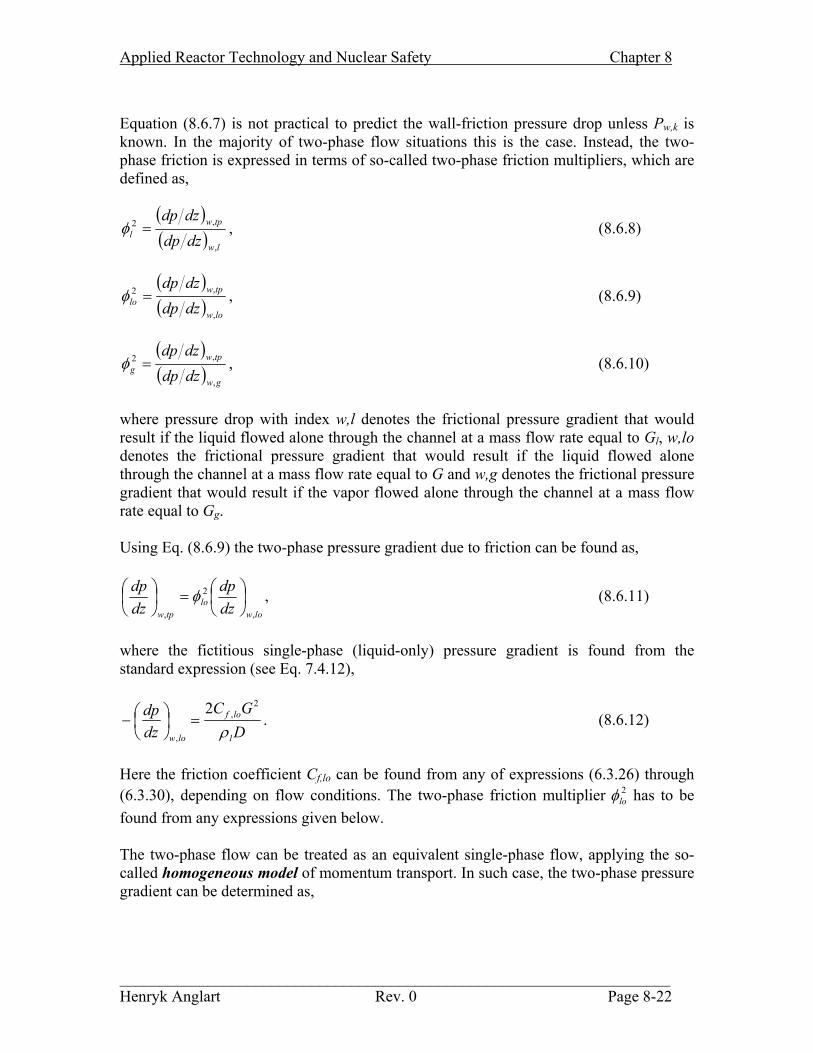
Equation (8.6.7) is not practical to predict the wall-friction pressure drop unless Pw,k is known. In the majority of two-phase flow situations this is the case. Instead, the two-phase friction is expressed in terms of so-called two-phase friction multipliers, which are defined as,
( )( ) lw
tpwl dzdp
dzdp
,
,2 =φ , (8.6.8)
( )( ) low
tpwlo dzdp
dzdp
,
,2 =φ , (8.6.9)
( )( ) gw
tpwg dzdp
dzdp
,
,2 =φ , (8.6.10)
where pressure drop with index w,l denotes the frictional pressure gradient that would result if the liquid flowed alone through the channel at a mass flow rate equal to Gl, w,lo denotes the frictional pressure gradient that would result if the liquid flowed alone through the channel at a mass flow rate equal to G and w,g denotes the frictional pressure gradient that would result if the vapor flowed alone through the channel at a mass flow rate equal to Gg. Using Eq. (8.6.9) the two-phase pressure gradient due to friction can be found as,
lowlo
tpw dzdp
dzdp
,
2
,
=
φ , (8.6.11)
where the fictitious single-phase (liquid-only) pressure gradient is found from the standard expression (see Eq. 7.4.12),
DGC
dzdp
l
lof
low ρ
2,
,
2=
− . (8.6.12)
Here the friction coefficient Cf,lo can be found from any of expressions (6.3.26) through (6.3.30), depending on flow conditions. The two-phase friction multiplier has to be found from any expressions given below.
2loφ
The two-phase flow can be treated as an equivalent single-phase flow, applying the so-called homogeneous model of momentum transport. In such case, the two-phase pressure gradient can be determined as,
_____________________________________________________________________ Henryk Anglart Rev. 0 Page 8-22

Applied Reactor Technology and Nuclear Safety Chapter 8
DGC
dzdp
m
tpf
tpw ρ
2,
,
2=
− . (8.6.13)
In this expression Cf,tp is an effective Fanning friction factor for the two-phase flow and
mρ is the mixture density. Combining Eqs. (8.6.11) through (8.6.13) yields,
−+== x
CC
CC
g
l
lof
tpf
m
l
lof
tpflo 11
,
,
,
,2
ρρ
ρρ
φ . (8.6.14)
The friction factors can usually be expressed as functions of the Reynolds number. Using Eq. (6.3.28) as a prototype of such a function, the friction factors read as follows,
b
m
btptpf
a
l
alolof
GDBBCGDAAC−
−
−
−
=⋅=
=⋅=
µµReRe ,, . (8.6.15)
Assuming next that coefficients in Eq. (8.6.15) for single-phase and two-phase are equal, that is A = B and a = b, Eq. (8.6.14) becomes,
−+
= x
g
l
b
l
mlo 112
ρρ
µµ
φ . (8.6.16)
The mixture viscosity appearing in Eqs. (8.6.15) and (8.6.16) can be defined in different ways. It is customary to use some kind of weighted mean value, employing quality as the weighting factor. Three examples of the mixture viscosity are as follows,
lgm
xxµµµ−
+=11 , (8.6.17)
( ) lgm xx µµµ −+= 1 , (8.6.18)
( )
l
l
g
g
m
m xxρ
µρµ
ρµ −
+=1
. (8.6.19)
Using Eq. (8.6.17) in (8.6.16), and taking a = b = 0.25 (see the Blasius correlation) yields,
−+
−+=
−
xxg
l
g
llo 1111
25.0
2
ρρ
µµφ (8.6.20)
Combining Eqs. (8.6.11), (8.6.12) and (8.6.20) yield the following expression for the friction pressure term:
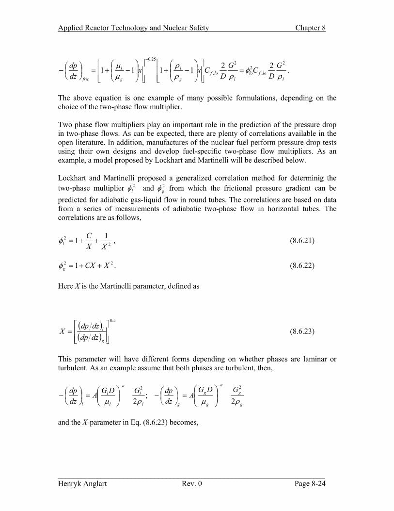
_____________________________________________________________________ Henryk Anglart Rev. 0 Page 8-23
Applied Reactor Technology and Nuclear Safety Chapter 8
lloflo
llof
g
l
g
l
fric
GD
CGD
Cxxdzdp
ρφ
ρρρ
µµ 2
,2
2
,
25.0221111 =
−+
−+=
−
−
.
The above equation is one example of many possible formulations, depending on the choice of the two-phase flow multiplier. Two phase flow multipliers play an important role in the prediction of the pressure drop in two-phase flows. As can be expected, there are plenty of correlations available in the open literature. In addition, manufactures of the nuclear fuel perform pressure drop tests using their own designs and develop fuel-specific two-phase flow multipliers. As an example, a model proposed by Lockhart and Martinelli will be described below. Lockhart and Martinelli proposed a generalized correlation method for determinig the two-phase multiplier and from which the frictional pressure gradient can be predicted for adiabatic gas-liquid flow in round tubes. The correlations are based on data from a series of measurements of adiabatic two-phase flow in horizontal tubes. The correlations are as follows,
2lφ
2gφ
22 11
XXC
l ++=φ , (8.6.21)
22 1 XCXg ++=φ . (8.6.22)
Here X is the Martinelli parameter, defined as
( )( )
5.0
=
g
l
dzdpdzdp
X (8.6.23)
This parameter will have different forms depending on whether phases are laminar or turbulent. As an example assume that both phases are turbulent, then,
g
g
a
g
g
gl
l
a
l
l
l
GDGA
dzdpGDGA
dzdp
ρµρµ 2;
2
22−−
=
−
=
−
and the X-parameter in Eq. (8.6.23) becomes,
_____________________________________________________________________ Henryk Anglart Rev. 0 Page 8-24

Applied Reactor Technology and Nuclear Safety Chapter 8
5.075.125.0
1
−
=
l
g
g
ltt x
xXρρ
µµ
The tt subscript indicates that both phases are turbulent. Other possible subscript combinations will be lt, tl and ll, meaning laminar liquid – turbulent vapor, turbulent liquid – laminar vapor and both phases laminar, respectively. The recommended value of the constant C in Eqs (8.6.21-22) differs, depending on the flow regime associated with the flow of the vapor and the liquid alone in the channel. There are four possible combinations in which each phase can be either laminar or turbulent. The values of C are shown in Table 8.6.1. Table 8.6.1. C constant for correlations (8.6.21) and (8.6.22). Liquid Gas -> Laminar Turbulent Laminar 5 12 Turbulent 10 20 The two phase flow multiplier can be expressed in terms of as follows, 2
loφ2lφ
( )( ) ( ) 275.1
,
,2 1 llow
tpwlo x
dzdpdzdp
φφ −== .
Gravity pressure drop: The gravity pressure drop term is defined as,
ϕρ singdzdp
mgrav
=
− .
Here sinφ=1 for vertical channels and sinφ=0 for horizontal channels. Since, in general, the mixture density ρm can change along channel, the pressure gradient will change accordingly. Acceleration pressure drop: The fourth term on the right-hand-side of Eq. (8.6.4) is termed as the acceleration pressure drop and can be evaluated as:
=
−
Macc
AGdzd
Adzdp
ρ
21
For constant G and A, this expression reduces to:
_____________________________________________________________________ Henryk Anglart Rev. 0 Page 8-25

Applied Reactor Technology and Nuclear Safety Chapter 8
=
−
Macc dzdG
dzdp
ρ12
Substituting the expression for the dynamic mixture density ρM into the above equation gives,
( )( )
−−
+=
−
lgacc
xxdzdG
dzdp
ρααρ 11 22
2
Equation (8.6.4) describes all pressure drop terms that appear in an arbitrary channel with two-phase flow which is smooth enough that there are no local pressure drops. If the channel contain local obstacles or sudden cross-section area changes, the corresponding pressure drops must be added to the previously described ones. This procedure is very much the same as that described in Chapter 7 for single-phase flows. However, some important differences, described below, have to be taken into account while applying the single-phase theory to two-phase flows. Local pressure drop: Local pressure losses for single phase have been discussed in Chapter 7. The single-phase flow theory will be now extended to two-phase flow situations. Using sections “1” and “2” shown in Fig. 7.4.1, the momentum balance equation can be written
( )( )[ 221122222222
11111111
1
1
ApApUAUUAU
UAUUAUF
ggggllll
ggggllll
−++− ]−+−=
ραρα
ραρα (8.6.24)
With similar arguments as for the single-phase flow case, the force F is taken equal to p1(A2-A1), and using s = A1/A2, Eq. (8.6.24) yields
( ) ( )
+
−−
−
+
−−
=−2
2
2
2
1
2
1
221
12 11
11
αρρ
ααρρ
αρxxsxxsGpp
g
l
g
l
l
. (8.6.25)
The corresponding irreversible pressure drop, assuming incompressible two-phase flow with ααα == 21 , becomes
( ) ( )( )
( )
−+
+
−−+
−
+
−−
−=∆−
lg
g
l
l
g
l
lI xx
xxsxxssGp
ρρ
αρρ
ρααρ
ραρ 1
11
21
111
3
22
3
2221 . (8.6.26)
It has been assumed that there is no phase change between sections “1” and “2”, that is x1 = x2. However, void fractions at the two sections are usually not equal to each other. It
_____________________________________________________________________ Henryk Anglart Rev. 0 Page 8-26

Applied Reactor Technology and Nuclear Safety Chapter 8
has been observed that void fraction significantly increases downstream of the enlargement. This effect disappears at some distance, however. This distance is evaluated to be between L/D = 10 up to 70. Nevertheless, Eq. (8.6.26) can be simplified by assuming the homogeneous model and the resultant irreversible pressure drop will become as follows,
lg
lI
GAAxp
ρρρ
2111
21
2
2
1
−
−+=∆− . (8.6.27)
This equation can be compared with its equivalent for the single-phase flow through a sudden enlargement given by Eq. (7.4.19). As can be seen, a new term appears, which can be identified as a two-phase multiplier for the local pressure loss
−+= 112
,g
ldlo x
ρρφ . (8.6.28)
The subscript lo,d is used to indicate that the multiplier given be Eq. (8.6.28) is valid for local losses, where the viscous effects can be neglected and only the density ratio between the two phases plays any role. The corresponding irreversible pressure drop for homogeneous two-phase flow through a sudden contraction becomes (see Section 7.4 for single-phase equivalent)
lcg
lI
GAAxp
ρρρ
2111
22
2
2
−
−+=∆− . (8.6.29)
Even here the two-phase multiplier (8.6.28) appears together with the local loss coefficient valid for single-phase flows (see Table 7.4.1 for values of the local loss coefficient). In general, a local irreversible pressure drop for two-phase flows can be expressed as
loIdlotpI pp ,2
,, ∆=∆ φ , (8.6.30) where tp stands for two-phase and lo for liquid only. As can be seen, the local pressure drop for two-phase flows can be obtained from a multiplication of the corresponding local pressure drop for single-phase flow and a proper two-phase multiplier. A similar principle is valid for the frictional pressure drop for single- and two-phase flows. It can be noted that the local two-phase multiplier given by Eq. (8.6.28) is not the same as the frictional two-phase multiplier, given by Eq. (8.6.20). The reason for this difference stems from the neglect of viscous losses in the case of the local pressure losses. Nevertheless, it should be mentioned that in many in practical calculations, the multiplier is assumed the same for both frictional and local pressure losses.
_____________________________________________________________________ Henryk Anglart Rev. 0 Page 8-27
Applied Reactor Technology and Nuclear Safety Chapter 8
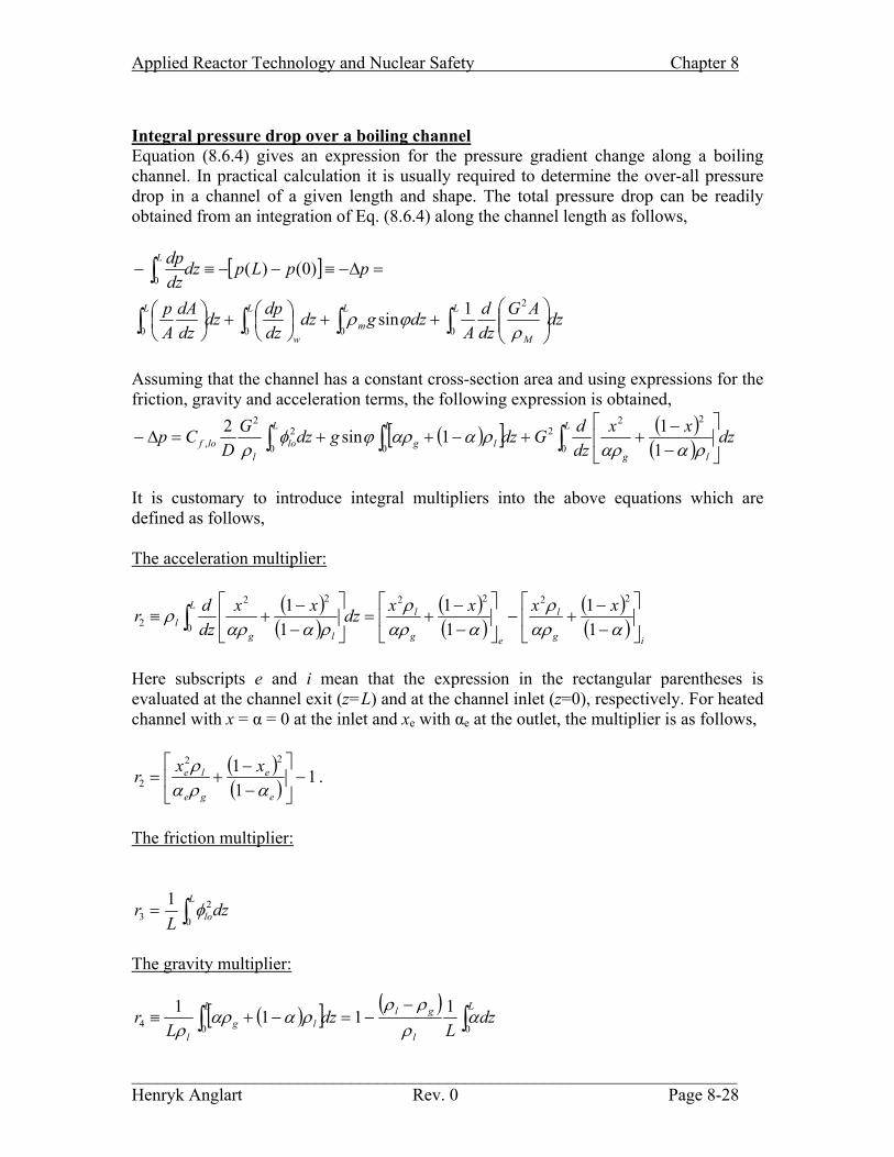
Integral pressure drop over a boiling channel Equation (8.6.4) gives an expression for the pressure gradient change along a boiling channel. In practical calculation it is usually required to determine the over-all pressure drop in a channel of a given length and shape. The total pressure drop can be readily obtained from an integration of Eq. (8.6.4) along the channel length as follows,
[ ]
dzAGdzd
Adzgdz
dzdpdz
dzdA
Ap
ppLpdzdzdp
L
M
L
m
L
w
L
L
∫∫∫∫
∫
++
+
=∆−≡−−≡−
0
2
000
0
1sin
)0()(
ρϕρ
Assuming that the channel has a constant cross-section area and using expressions for the friction, gravity and acceleration terms, the following expression is obtained,
( )[ ] ( )( ) dzxx
dzdGdzgdzG
DCp
L
lg
L
lg
L
lol
lof ∫∫∫
−−
++−++=∆−0
222
00
22
, 111sin2
ρααρρααρϕφ
ρ
It is customary to introduce integral multipliers into the above equations which are defined as follows, The acceleration multiplier:
( )( )
( )( )
( )( )
ig
l
eg
lL
lgl
xxxxdzxxdzdr
−−
+−
−−
+=
−−
+≡ ∫ ααρρ
ααρρ
ρααρρ
11
11
11 2222
0
22
2
Here subscripts e and i mean that the expression in the rectangular parentheses is evaluated at the channel exit (z=L) and at the channel inlet (z=0), respectively. For heated channel with x = α = 0 at the inlet and xe with αe at the outlet, the multiplier is as follows,
( )( ) 111 22
2 −
−−
+=e
e
ge
le xxrαρα
ρ .
The friction multiplier:
dzL
rL
lo∫=0
23
1 φ
The gravity multiplier:
( )[ ] ( )dz
Ldz
Lr
L
l
glL
lgl
∫∫−
−=−+≡004
1111 αρρρ
ρααρρ
_____________________________________________________________________ Henryk Anglart Rev. 0 Page 8-28
Applied Reactor Technology and Nuclear Safety Chapter 8
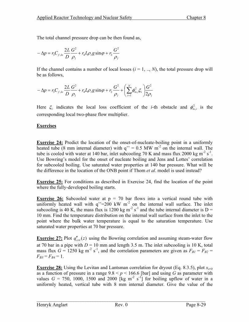
The total channel pressure drop can be then found as,
ll
llof
GrgLrGDLCrp
ρϕρ
ρ
2
24
2
,3 sin2++=∆−
If the channel contains a number of local losses (i = 1, .., N), the total pressure drop will be as follows,
l
N
iiilo
ll
llof
GGrgLrGDLCrp
ρξφ
ρϕρ
ρ 2sin2 2
1
2,
2
24
2
,3
+++=∆− ∑=
Here iξ indicates the local loss coefficient of the i-th obstacle and is the corresponding local two-phase flow multiplier.
2,iloφ
Exercises Exercise 24: Predict the location of the onset-of-nucleate-boiling point in a uniformly heated tube (8 mm internal diameter) with q’’ = 0.5 MW m-2 on the internal wall. The tube is cooled with water at 140 bar, inlet subcooling 70 K and mass flux 2000 kg m-2 s-1. Use Bowring’s model for the onset of nucleate boiling and Jens and Lottes’ correlation for subcooled boiling. Use saturated water properties at 140 bar pressure. What will be the difference in the location of the ONB point if Thom et al. model is used instead? Exercise 25: For conditions as described in Exercise 24, find the location of the point where the fully-developed boiling starts. Exercise 26: Subcooled water at p = 70 bar flows into a vertical round tube with uniformly heated wall with q’’=200 kW m-2 on the internal wall surface. The inlet subcooling is 40 K, the mass flux is 1200 kg m-2 s-1 and the tube internal diameter is D = 10 mm. Find the temperature distribution on the internal wall surface from the inlet to the point where the bulk water temperature is equal to the saturation temperature. Use saturated water properties at 70 bar pressure. Exercise 27: Plot using the Bowring correlation and assuming steam-water flow at 70 bar in a pipe with D = 10 mm and length 3.5 m. The inlet subcooling is 10 K, total mass flux G = 1250 kg m
)(zqcrit′′
-2 s-1, and the correlation parameters are given as FB1 = FB2 = FB3 = FB4 = 1. Exercise 28: Using the Levitan and Lantsman correlation for dryout (Eq. 8.3.5), plot xcrit as a function of pressure in a range 9.8 < p < 166.6 [bar] and using G as parameter with values G = 750, 1000, 1500 and 2000 [kg m-2 s-1] for boiling upflow of water in a uniformly heated, vertical tube with 8 mm internal diameter. Give the value of the
_____________________________________________________________________ Henryk Anglart Rev. 0 Page 8-29

Applied Reactor Technology and Nuclear Safety Chapter 8
_____________________________________________________________________ Henryk Anglart Rev. 0 Page 8-30
pressure for which xcrit becomes maximum. Use this pressure to plot xcrit as a function of G. Exercise 29: Calculate the heat transfer coefficient from the Groeneveld correlation (Eq. 8.4.5) for steam-water flow in a vertical tube: D = 10 mm, G = 1200 kg m-2 s-1, p = 70 bar, heat flux q = 1.0 MW m-2 at axial positions where x = 0.2, 0.4, 0.6 and 0.8. Assume that the vapor Prandtl number varies with the temperature as Pr(T) = 1.05 -8*(T-623)*10-4 , where T is in [K]. Check whether the validity ranges are satisfied. Exercise 30: Plot void fraction in function of flow quality (in a range from 0 to 1) assuming flow of water and vapor mixture at saturation conditions and at pressure p = 70 bar. Compare two cases: in one case both phases have the same averaged velocity; in the other case the vapor phase flows with mean velocity which is 20% higher than the mean liquid velocity. Exercise 31: Compare void fraction predicted from the homogeneous model and the drift-flux model for steam-water flow. Assume p = 70 bar, G = 1200 kg m-2 s-1 and Eqs (8.5.2-11) and (8.5.2-12) for drift-flux parameters. Plot void fraction in function of quality. Plot slip ratio given by Eq. (8.5.2-14) in function of quality for the same conditions. Exercise 32: Plot two-phase multiplier (8.6.20) as a function of quality assuming two-phase flow of water-vapor mixture under 70 bar pressure. Exercise 33: Plot two-phase multipliers (8.6.16) using three different definitions of mixture viscosity. Assume same conditions as in Exercise 32. Exercise 34: Derive expressions for integral multipliers r2, r3 and r4 for channels with saturated liquid at the inlet and with uniform heat flux distribution along channel length. Hint: in integrals along channel length use substitution: dz = const * dx, which is valid for uniformly heated channels. Exercise 35: Solve Exercise 23 assuming constant heat flux applied to the channel and equal to 3 MW m-2. Home Assignment # 4 (due to 05.02.16) Vertical smooth pipe with 8 mm internal diameter and length 3.6 m is uniformly heated with heat flux q’’ = 0.75 MW/m2. The pipe is cooled with water flowing vertically upwards, with inlet pressure 150 bar, inlet subcooling 70 K and mass flux 1000 kg m-2 s-1. Use saturated water properties at 150 bar pressure. Problem 1 (5 points): Using the Bowring’s model for the onset of nucleate boiling and Jens&Lottes correlation for the subcooled boiling predict the locations of the Onset of Nucleate Boiling (znb) and the Fully Developed Boiling (zfdb) in the channel. Problem 2 (5 points): Using the homogeneous equilibrium model (HEM) calculate the total pressure drop in the channel.