8 The HIRM+ Flight Dynamics Model - DLR Portalelib.dlr.de/12205/1/moormann_lncis02.pdf · 8 The HIRM+ Flight Dynamics Model Dieter Moormann EADS Deutschland GmbH??, Military Aircraft

8 The HIRM+ Flight Dynamics Model

Dieter Moormann

EADS Deutschland GmbH??, Military AircraftMT62 Flight Dynamcis, 81663 Munchen, [email protected]

Summary. The major objective of the GARTEUR Action Group on AnalysisTechniques for Clearance of Flight Control Laws FM(AG-11) is the improvementof the flight clearance process by increased automation of the tools used for model-based analysis of the aircraft’s dynamical behaviour. What is finally needed aretechniques for faster detection of the worst case combination of parameter valuesand manoeuvre cases, from which the flight clearance restrictions are be derived.The basis for such an analysis are accurate mathematical models of the controlledaircraft. In this chapter the HIRM+ flight dynamics model is described as one ofthe benchmark military aircraft models used within FM(AG-11). HIRM+ originatesfrom the HIRM (High Incidence Research Model) developed within the GARTEURAction Group on Robust Flight Control FM(AG-08). In building the HIRM+, ad-ditional emphasis has been put on realistic modelling of parametric uncertainties.

8.1 Introduction

The HIRM+ has been developed from the HIRM, a mathematical model ofa generic fighter aircraft originally developed by the Defence and EvaluationResearch Agency (DERA, Bedford). The HIRM is based on aerodynamic dataobtained from wind tunnel tests and flight testing of an unpowered, scaleddrop model. The model was set up to investigate flights at high angles of at-tack (-50◦ ≤ α ≤ 120◦) and over a wide sideslip range (- 50◦ ≤ β ≤ +50◦), butdoes not include compressibility effects resulting from high subsonic speeds.The origin of the model explains the unconventional configuration with bothcanard and tailplane, plus an elongated nose (see Fig. 8.1).

The aircraft is basically stable. However, there are combinations of angleof attack and control surface deflections, which cause the aircraft to becomeunstable longitudinally and/or laterally. Engine, actuator and sensor dyna-mics models have been added within FM-AG-08 to create a representative,nonlinear simulation model of a twin-engined, modern fighter aircraft. Themodel building was done by using the object-oriented equation-based model-ling environment Dymola [4].

?? The work on this project was conducted while the author was employed at DLR,Institute of Robotics and Mechatronics, Oberpfaffenhofen, 82234 Wessling, Ger-many

122 Dieter Moormann

Fig. 8.1. High Incidence Research Model [1]

In building the HIRM+, the emphasis has been put on realistic modellingof parametric uncertainties. Parameters have been defined to specify uncer-tainties in mass, inertial data, position of the centre of gravity, aerodynamiccontrol power derivatives, stability derivatives, and some coefficients in theactuator and engine dynamics. In spite of these changes, the nominal modelsof HIRM+ and HIRM (i.e., with all uncertain parameters set to zero) areessentially the same.

Although variations of the uncertainty parameters affect the trim valuesof states and control surface deflections, due to the HIRM’s fairly linear aero-dynamic derivatives over the specified flight envelope, the stability propertiesremain essentially unchanged

Another aspect arising from the current industrial clearance practice isto allow the use of expected tolerance ranges of typical uncertain parameters(e.g., stability and control power derivatives) to be directly accessible in thenonlinear model. This allows the HIRM+ to mimic the industrial clearanceapproach, which is heavily based on both linear and nonlinear aircraft models.Usually, individual entries of the state-space matrices, with known physicalmeaning, are considered as uncertain and varied within the expected ranges.

8 The HIRM+ Flight Dynamics Model 123

automaticcode generation

aerodynamic controls& engine controls& gust inputs

measurements& evaluation outputs

Fig. 8.2. The HIRM+ aircraft dynamics model

8.2 The HIRM+ Object Model

The HIRM+ aircraft dynamics model in the upper part of Figure 8.2 consistsof four basic blocks denoted as: actuator dynamics, engine dynamics, flightdynamics and sensor dynamics. Zooming into the flight dynamics model dis-plays its internal structure, as given in the lower half of Fig. 8.2: The flight dy-namics block incorporates the mass properties including equations of motionand the models of aerodynamics, variations in thrust, gravity, atmosphere,and gust disturbances [2, 3].

124 Dieter Moormann

In contrast to the (input-output) block-oriented description of the air-craft dynamics model, the flight dynamics model itself is specified using anacausal model formulation [4]. Due to the acausal approach, interconnectionsbetween components are not limited to signal flows but represent physicalsystem interactions, like energy flows, or kinematic constraints. Automaticcode generation is used to import the flight dynamics into the overall model.

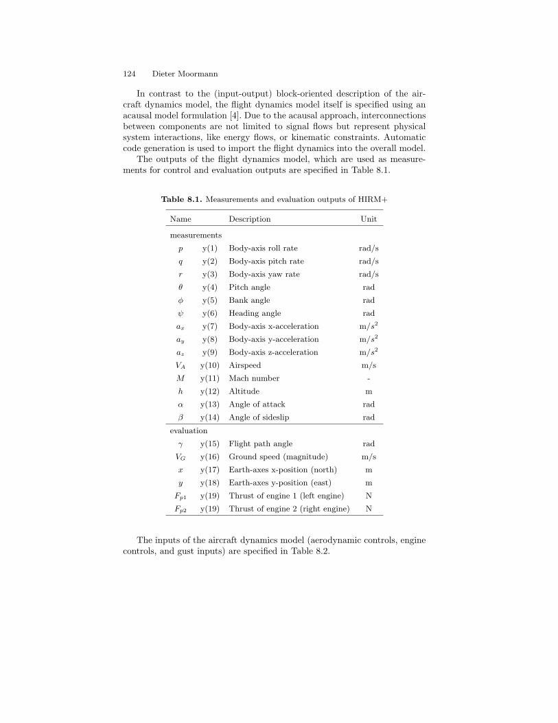
The outputs of the flight dynamics model, which are used as measure-ments for control and evaluation outputs are specified in Table 8.1.

Table 8.1. Measurements and evaluation outputs of HIRM+

Name Description Unit

measurements

p y(1) Body-axis roll rate rad/s

q y(2) Body-axis pitch rate rad/s

r y(3) Body-axis yaw rate rad/s

θ y(4) Pitch angle rad

φ y(5) Bank angle rad

ψ y(6) Heading angle rad

ax y(7) Body-axis x-acceleration m/s2

ay y(8) Body-axis y-acceleration m/s2

az y(9) Body-axis z-acceleration m/s2

VA y(10) Airspeed m/s

M y(11) Mach number -

h y(12) Altitude m

α y(13) Angle of attack rad

β y(14) Angle of sideslip rad

evaluation

γ y(15) Flight path angle rad

VG y(16) Ground speed (magnitude) m/s

x y(17) Earth-axes x-position (north) m

y y(18) Earth-axes y-position (east) m

Fp1 y(19) Thrust of engine 1 (left engine) N

Fp2 y(19) Thrust of engine 2 (right engine) N

The inputs of the aircraft dynamics model (aerodynamic controls, enginecontrols, and gust inputs) are specified in Table 8.2.


Table 8.2. Controls and gust inputs of HIRM+

Name Description Unit

δTS u(1) Symmetric tailplane deflection rad

δTD u(2) Differential tailplane deflection rad

δCS u(3) Symmetric canard deflection rad

δCD u(4) Differential canard deflection rad

δR u(5) Rudder deflection rad

suction u(6) Nose suction -

δTH1 u(7) Throttle of engine 1 (left engine) -

δTH2 u(8) Throttle of engine 2 (right engine) -

WXB u(9) Body-axes head wind m/s

WYB u(10) Body-axes cross wind m/s

WZB u(11) Body-axes vertical wind m/s

The uncertain parameters of the HIRM+, their formulation, nominal val-ues, upper and lower bounds, units and descriptions are given in sections8.2.1 to 8.2.5.

8.2.1 Mass characteristics and geometric data

The body-object of Fig. 8.2 specifies the mass characteristics and the rigidbody differential equations of motion with 6 degrees of freedom. For a deriva-tion of these equations a reference such as [5] should be consulted.

The HIRM+ mass characteristics are specified in Table 8.3Variations in mass and moment of inertia are given by the following equa-

tions. For convenience, the uncertain parameters of the HIRM+ are denotedwith an asterisk and parameters without, as their nominal values. The un-certainty itself is expressed by the subscript Unc:

m∗ = (mUnc + 1) m

I∗ =

Ix(1 + IxUnc) 0 −Ixz(1 + IxzUnc

)0 Iy(1 + IyUnc) 0

Ixz(1 + IxzUnc) 0 Iz(1 + IzUnc)

The centre of gravity varies with respect to its nominal value which isdefined as body geometric reference BGR, see Fig. 8.2):

X∗cg = Xcg + XcgUnc

Y ∗cg = Ycg + YcgUnc

Z∗cg = Zcg + ZcgUnc

126 Dieter Moormann

Table 8.3. Inertial parameters

Name Nominal value Unit Description

m 15296.0 kg Aircraft total mass

Ix 24549.0 kg m2 x body moment of inertia

Iy 163280.0 kg m2 y body axis moment of inertia

Iz 183110.0 kg m2 z body moment of inertia

Ixz -3124.0 kg m2 x-z body axis product of inertia

Xcg 0 m Centre of gravity location along x-axis

w.r.t. body geometric reference BGR

Ycg 0 m Centre of gravity location along y-axis


Zcg 0 m Centre of gravity location along z-axis


Table 8.4. Inertial uncertain parameters

Name Nominal [min; max] Unit Description

value

mUnc 0 [-0.2; 0.2] - Uncertainty level of aircraft mass

XcgUnc 0 [-0.15; 0.15] m Centre of Gravity offset alongx-axis from nominal Xcg, positivetoward nose

YcgUnc 0 [-0.10; 0.10] m Centre of Gravity offset alongy-axis from nominal Ycg, positivetoward starboard

ZcgUnc 0 [-0.04; 0.04] m Centre of Gravity offset alongz-axis from nominal Zcg, positivedown

IxUnc 0 [-0.2; 0.2] - Uncertainty level of Ix

IyUnc 0 [-0.05; 0.05] - Uncertainty level of Iy

IzUnc 0 [-0.08; 0.08] - Uncertainty level of Iz

IxzUnc 0 [-0.2; 0.2] - Uncertainty level of Ixz

The parametric uncertainties in the HIRM+ mass characteristics are de-fined using the parameters given in Table 8.4 in terms of their nominal values(see Table 8.3) and their set of uncertain parameters.


In some cases (e.g. mass) physical units are not shown, because the uncer-tainties are expressed in terms of percentages (±20% for mass) of the nominalvalue.

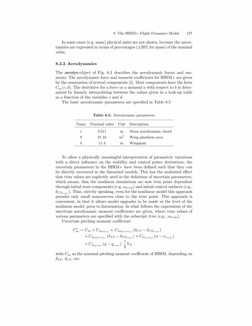
8.2.2 Aerodynamics

The aerodyn-object of Fig. 8.2 describes the aerodynamic forces and mo-ments. The aerodynamic force and moment coefficients for HIRM+ are givenby the summation of several components [1]. Most components have the formCab

(c, d). The derivative for a force or a moment a with respect to b is deter-mined by linearly interpolating between the values given in a look-up tableas a function of the variables c and d.

The basic aerodynamic parameters are specified in Table 8.5

Table 8.5. Aerodynamic parameters

Name Nominal value Unit Description

c 3.511 m Mean aerodynamic chord

S 37.16 m2 Wing planform area

b 11.4 m Wingspan

To allow a physically meaningful interpretation of parametric variationswith a direct influence on the stability and control power derivatives, theuncertain parameters in the HIRM+ have been defined such that they canbe directly recovered in the linearised models. This has the undesired effectthat trim values are explicitly used in the definition of uncertain parameters,which means, that the nonlinear simulations are now trim point dependentthrough initial state components (e.g.,αtrim) and initial control surfaces (e.g.,δCStrim). Thus, strictly speaking, even for the nonlinear model this approachpermits only small manoeuvres close to the trim point. This approach isconvenient, in that it allows model upgrades to be made at the level of thenonlinear model, prior to linearisation. In what follows the expressions of theuncertain aerodynamic moment coefficients are given, where trim values ofvarious parameters are specified with the subscript trim (e.g., αtrim).

Uncertain pitching moment coefficient:

C∗m = Cm + Cm0 Unc+ CmδCS Unc

(δCS − δCStrim)+ CmδT S Unc

(δTS − δTStrim) + Cmα Unc(α− αtrim)

+ Cmq Unc (q − qtrim)c

2VA

with Cm as the nominal pitching moment coefficient of HIRM, depending onδTS , δCS , etc.

128 Dieter Moormann

Uncertain rolling moment coefficient:

C∗l = Cl + Cl0 Unc+ ClδCD Unc

(δCD − δCDtrim)

+ ClδT D Unc(δTD − δTDtrim) + ClδR Unc

(δR − δRtrim)

+ Clβ Unc(β − β

trim) + Clr Unc

rb

2 VA+ Clp Unc

pb

2 VA

with Cl as the nominal rolling moment coefficient of HIRM.Uncertain yawing moment coefficient:

C∗n = Cn + Cn0 Unc+ CnδCD Unc

(δCD − δCDtrim)

+ CnδT D Unc(δTD − δTDtrim) + CnδR Unc

(δR − δRtrim)

+ Cnβ Unc(β − β

trim) + Cnr Unc

rb

2 VA+ Cnp Unc

pb

2 VA

with Cn as the nominal yawing moment coefficient of HIRM.

Table 8.6. Uncertain parameters of aerodynamic stability derivatives

Name Nom. [min; max] Unit Description

value

Cl0 Unc 0 [0 ; 0] - Uncertainty in rolling moment

Cm0 Unc 0 [0 ; 0] - Uncertainty in pitching moment

Cn0 Unc 0 [0 ; 0] - Uncertainty in yawing moment

Cmα Unc 0 [-0.1; 0.1] 1/rad Uncertainty in Cmα stability derivative

Clβ Unc 0 [-0.04; 0.04] 1/rad Uncertainty in Clβ stability derivative,where: k = 1 for α < 12◦, k = 2 forα > 20◦, and k is linearly interpolatedfor 12◦ ≤ α ≤ 20◦ between 1 and 2.

Cnβ Unc 0 [-0.04; 0.04] 1/rad Uncertainty in Cnβ stability derivative

Cmq Unc 0 [-0.1; 0.1] - Uncertainty in pitching moment deriva-tive due to normalised pitch rate

Clp Unc 0 [-0.1; 0.1] - Uncertainty in rolling moment deriva-tive due to normalised roll rate

Clr Unc 0 [-0.03; 0.03] - Uncertainty in rolling moment deriva-tive due to normalised yaw rate

Cnp Unc 0 [-0.1; 0.1] - Uncertainty in yawing moment deriva-tive due to normalised roll rate

Cnr Unc 0 [-0.05; 0.05] - Uncertainty in yawing moment deriva-tive due to normalised yaw rate

In Tables 8.6 and 8.7 the ranges of the uncertain aerodynamic stabilityderivatives and control power derivatives are given. For some parameters, no


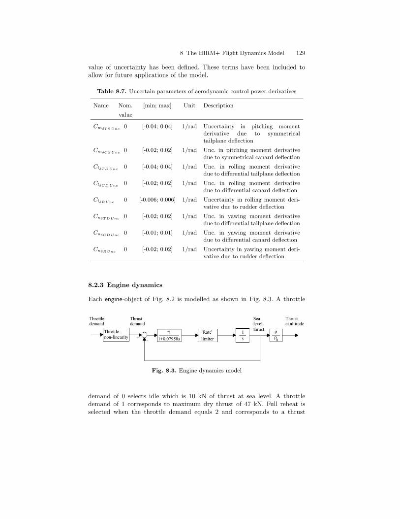
value of uncertainty has been defined. These terms have been included toallow for future applications of the model.

Table 8.7. Uncertain parameters of aerodynamic control power derivatives

Name Nom. [min; max] Unit Description

value

CmδT S Unc 0 [-0.04; 0.04] 1/rad Uncertainty in pitching momentderivative due to symmetricaltailplane deflection

CmδCS Unc 0 [-0.02; 0.02] 1/rad Unc. in pitching moment derivativedue to symmetrical canard deflection

ClδT D Unc 0 [-0.04; 0.04] 1/rad Unc. in rolling moment derivativedue to differential tailplane deflection

ClδCD Unc 0 [-0.02; 0.02] 1/rad Unc. in rolling moment derivativedue to differential canard deflection

ClδR Unc 0 [-0.006; 0.006] 1/rad Uncertainty in rolling moment deri-vative due to rudder deflection

CnδT D Unc 0 [-0.02; 0.02] 1/rad Unc. in yawing moment derivativedue to differential tailplane deflection

CnδCD Unc 0 [-0.01; 0.01] 1/rad Unc. in yawing moment derivativedue to differential canard deflection

CnδR Unc 0 [-0.02; 0.02] 1/rad Uncertainty in yawing moment deri-vative due to rudder deflection

8.2.3 Engine dynamics

Each engine-object of Fig. 8.2 is modelled as shown in Fig. 8.3. A throttle

Fig. 8.3. Engine dynamics model

demand of 0 selects idle which is 10 kN of thrust at sea level. A throttledemand of 1 corresponds to maximum dry thrust of 47 kN. Full reheat isselected when the throttle demand equals 2 and corresponds to a thrust

130 Dieter Moormann

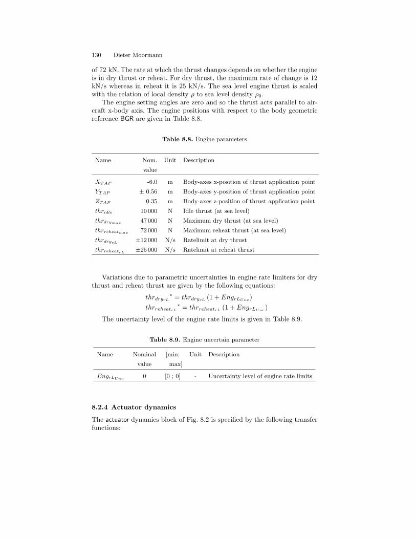
of 72 kN. The rate at which the thrust changes depends on whether the engineis in dry thrust or reheat. For dry thrust, the maximum rate of change is 12kN/s whereas in reheat it is 25 kN/s. The sea level engine thrust is scaledwith the relation of local density ρ to sea level density ρ0.

The engine setting angles are zero and so the thrust acts parallel to air-craft x-body axis. The engine positions with respect to the body geometricreference BGR are given in Table 8.8.

Table 8.8. Engine parameters

Name Nom. Unit Description

value

XTAP -6.0 m Body-axes x-position of thrust application point

YTAP ± 0.56 m Body-axes y-position of thrust application point

ZTAP 0.35 m Body-axes z-position of thrust application point

thridle 10 000 N Idle thrust (at sea level)

thrdrymax 47 000 N Maximum dry thrust (at sea level)

thrreheatmax 72 000 N Maximum reheat thrust (at sea level)

thrdryrL ±12 000 N/s Ratelimit at dry thrust

thrreheatrL ±25 000 N/s Ratelimit at reheat thrust

Variations due to parametric uncertainties in engine rate limiters for drythrust and reheat thrust are given by the following equations:

thrdryrL

∗ = thrdryrL (1 + EngrLUnc)thrreheatrL

∗ = thrreheatrL (1 + EngrLUnc)

The uncertainty level of the engine rate limits is given in Table 8.9.

Table 8.9. Engine uncertain parameter

Name Nominal [min; Unit Description

value max]

EngrLUnc 0 [0 ; 0] - Uncertainty level of engine rate limits

8.2.4 Actuator dynamics

The actuator dynamics block of Fig. 8.2 is specified by the following transferfunctions:


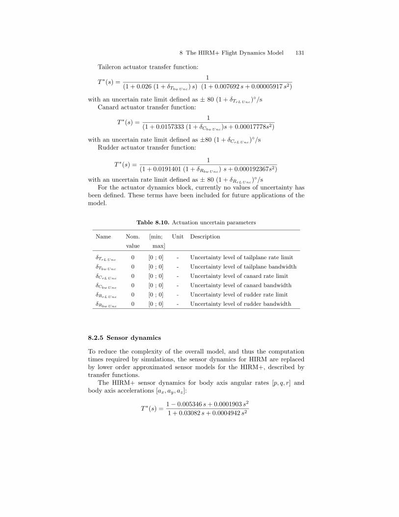
Taileron actuator transfer function:

T ∗(s) =1

(1 + 0.026 (1 + δTbw Unc) s) (1 + 0.007692 s + 0.00005917 s2)

with an uncertain rate limit defined as ± 80 (1 + δTrL Unc)◦/s

Canard actuator transfer function:

T ∗(s) =1

(1 + 0.0157333 (1 + δCbw Unc)s + 0.00017778s2)

with an uncertain rate limit defined as ±80 (1 + δCrL Unc)◦/s

Rudder actuator transfer function:

T ∗(s) =1

(1 + 0.0191401 (1 + δRbw Unc) s + 0.000192367s2)

with an uncertain rate limit defined as ± 80 (1 + δRrL Unc)◦/s

For the actuator dynamics block, currently no values of uncertainty hasbeen defined. These terms have been included for future applications of themodel.

Table 8.10. Actuation uncertain parameters

Name Nom. [min; Unit Description

value max]

δTrL Unc 0 [0 ; 0] - Uncertainty level of tailplane rate limit

δTbw Unc 0 [0 ; 0] - Uncertainty level of tailplane bandwidth

δCrL Unc 0 [0 ; 0] - Uncertainty level of canard rate limit

δCbw Unc 0 [0 ; 0] - Uncertainty level of canard bandwidth

δRrL Unc 0 [0 ; 0] - Uncertainty level of rudder rate limit

δRbw Unc 0 [0 ; 0] - Uncertainty level of rudder bandwidth

8.2.5 Sensor dynamics

To reduce the complexity of the overall model, and thus the computationtimes required by simulations, the sensor dynamics for HIRM are replacedby lower order approximated sensor models for the HIRM+, described bytransfer functions.

The HIRM+ sensor dynamics for body axis angular rates [p, q, r] andbody axis accelerations [ax, ay, az]:

T ∗(s) =1− 0.005346 s + 0.0001903 s2

1 + 0.03082 s + 0.0004942 s2

132 Dieter Moormann

The HIRM+ sensor dynamics for airspeed, Mach-number, altitude, angleof attack and angle of sideslip [VA, Ma, h, α, β]:

T ∗(s) =1

1 + 0.02 s

The HIRM+ sensor dynamics for body axis attitudes and heading angle[ϕ, θ, ψ]:

T ∗(s) =1

1 + 0.0323 s + 0.00104 s2

A measurement error signal is added to the signal of α and β. These errorsare assumed to be constant during the period of simulation:

α∗ = α + αUnc

β∗ = β + βUnc

For the HIRM+ sensor dynamics block, currently no value of uncertaintyfor α- and β-measurement errors have been defined. These terms have beenincluded for compatibility with the HIRM, in which these uncertainties hadbeen used.

Table 8.11. Sensor uncertain parameters

Name nom [min; max] Unit Description

αUnc 0 [0 ; 0] [rad] Uncertainty in sensed angle of attack(added to the α-measurement signal)

βUnc 0 [0 ; 0] [rad] Uncertainty in sensed sideslip angle(added to the β-measurement signal)

8.3 Automated Model Generation for Parametric TimeSimulations and Trim Computations

The object model in Fig. 8.2 is graphically specified using components fromthe Flight Dynamics Library [3], that are instantiated with HIRM+ specificsystem model parameters. From this object model, simulation and analysismodels of the aircraft system dynamics and documentation can be generatedautomatically (see Fig. 8.4).

In the mathematical model building process, the equation handler of Dy-mola solves the equations according to the inputs and outputs of the com-plete HIRM+ model. Equations that are formulated in an object, but that


simulation model

mathematical

code-generation

physical model physical system model

system- parameter

trim code

component libraries

model building

specification ofmodel inputs andoutputs

e.g. Matlab/Simulink- (cmex-) S-function

(automatic)

e.g. Matlab/Simulink- (cmex-) S-function

modelling

u y u y8 8

sorted & solvedequations for

simulation

sorted & solvedequations for

trim calculation

composition

(interactive)

(automatic)

dtsdtddr

Valphabetaqgamma

Valphabeta

dtsdtddrthrottle1throttle2

15296.0

3.511

Fig. 8.4. Model building process

are superfluous for capturing the behaviour of the particular model, are auto-matically removed. The result is a nonlinear symbolic state-space descriptionwith a minimum number of equations for this task

x = f(x, u, p)y = h(x, u, p)

From the symbolic description, numerical simulation code for differentsimulation environments is generated automatically. In this way, it is possibleto generate, for example, a Matlab-Simulink m-file or cmex-code, or C-Code according to the neutral DSblock standard [7], which can be used inany simulation environment, being capable of importing C-Code.

From the sorted and solved equations for simulation, symbolic analysiscode can be generated, describing a parameterised state-space model. This

134 Dieter Moormann

code can be used to extract in an automated procedure the so-called LinearFractional Transformation (LFT) standard form, that may serve as the basisfor µ robustness analysis. A detailed description of the generation of an LFTrepresentation from an object model as depicted in Fig. 8.4 can be foundin [8].

One of the key aspects of the successful usage of an optimisation-basedclearance methodology is an efficient trimming approach. The trimming ofHIRM+ is a very challenging computational task, involving the numericalsolution of a system of 60 nonlinear equations for the stationary values of stateand control variables appearing in the HIRM+ state model. The difficultiesmainly arise because of the lack of differentiability of the functions due tothe presence of various look-up tables used for linear interpolations. Severenonlinearities in the engine model and in the aerodynamics, as well as thepresence of control surface deflection limiters make the numerical solution ofthis high order system of equations very difficult.

To manage the trimming problem, an highly accurate and efficient ap-proach has been employed in [2]. The facilities of an equation based modellingenvironment as Dymola [4] allows the generation of C-code for an inversemodel to serve for trimming. Such a model has as inputs the desired trimconditions (such as Va, α, . . . ) and as outputs the corresponding equilibriumvalues of trimmed state (x) and control vectors (such as δTS , δCS ,. . . ). Dy-mola generates essentially explicit equations for the inverse model by tryingto solve the 60th order nonlinear equation symbolically. Even if a symbolicsolution cannot be determined, Dymola is still able to reduce the burden ofsolving numerically a 60th order system of nonlinear equations to the solutionof a small core system of 13 nonlinear equations which ultimately must besolved numerically. Thus, the trimming procedure based on such an inversemodel is very fast and very accurate.

8.4 Flight Conditions and Envelope Limits

The analysis of HIRM+ is restricted to the flight conditions defined in Table8.12. Depending on the clearance problem, the equilibrium conditions in these

Table 8.12. Set of flight conditions for clearance analysis

FC No. FC1 FC2 FC3 FC4 FC5 FC6 FC7 FC8

M 0.2 0.3 0.5 0.5 0.6 0.7 0.8 0.8

h [ft] 5,000 25,000 40,000 15,000 30,0000 20,000 5,000 40,000

points are defined by the trimming conditions for straight and level flight forgiven γ, M and h or pull-up manoeuvres for given α, M and h. For the


variation of the α the interval [−15◦, 35◦] has been chosen, and for griddinga step size ∆α = 2◦ has been suggested.

When several aerodynamic uncertainties are simultaneously used in theanalysis, reduction factors must be applied on their absolute values as speci-fied in Tables 8.6 and 8.7. The values of reduction factors for different numbersof aerodynamic uncertainties are given in Table 8.13.

Table 8.13. Reduction factors for simultaneous aerodynamic uncertainties

Number of aerodynamic uncertainties 2 3 4 ≥ 5

Reduction factor 0.62 0.46 0.37 0.31

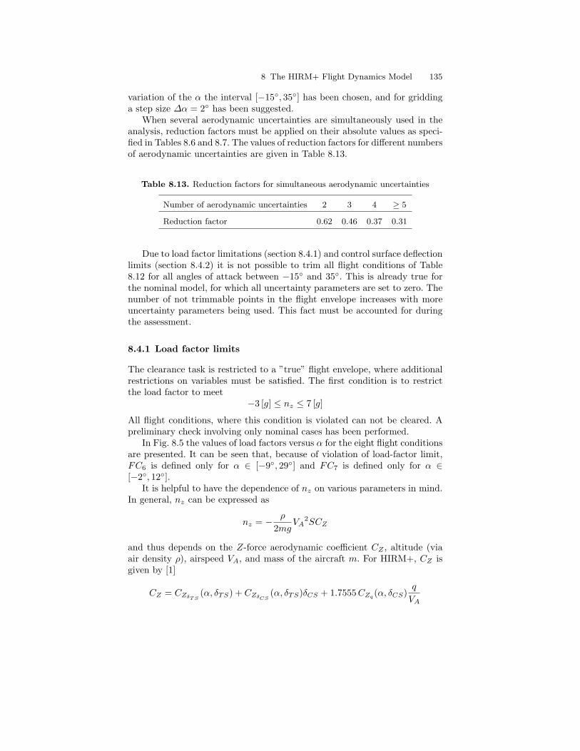
Due to load factor limitations (section 8.4.1) and control surface deflectionlimits (section 8.4.2) it is not possible to trim all flight conditions of Table8.12 for all angles of attack between −15◦ and 35◦. This is already true forthe nominal model, for which all uncertainty parameters are set to zero. Thenumber of not trimmable points in the flight envelope increases with moreuncertainty parameters being used. This fact must be accounted for duringthe assessment.

8.4.1 Load factor limits

The clearance task is restricted to a ”true” flight envelope, where additionalrestrictions on variables must be satisfied. The first condition is to restrictthe load factor to meet

−3 [g] ≤ nz ≤ 7 [g]

All flight conditions, where this condition is violated can not be cleared. Apreliminary check involving only nominal cases has been performed.

In Fig. 8.5 the values of load factors versus α for the eight flight conditionsare presented. It can be seen that, because of violation of load-factor limit,FC6 is defined only for α ∈ [−9◦, 29◦] and FC7 is defined only for α ∈[−2◦, 12◦].

It is helpful to have the dependence of nz on various parameters in mind.In general, nz can be expressed as

nz = − ρ

2mgVA

2SCZ

and thus depends on the Z-force aerodynamic coefficient CZ , altitude (viaair density ρ), airspeed VA, and mass of the aircraft m. For HIRM+, CZ isgiven by [1]

CZ = CZδT S(α, δTS) + CZδCS

(α, δTS)δCS + 1.7555 CZq (α, δCS)q

VA

136 Dieter Moormann

−15 −10 −5 0 5 10 15 20 25 30 35−10

−5

−3

0

5

7

10

15

20 Load factors for nominal cases

nz

AoA [deg]

FC1

FC2

FC3

FC4

FC5

FC6

FC7

FC8

Fig. 8.5. Nominal load factors for HIRM+

Because δCS = 0◦ (the canards are not used) and the term 1.7555 CZq (α, δCS) qVA

being much smaller than CZδT S, CZ can be approximated by the single term

CZ ≈ CZδT S(α, δTS), where the dependence on δTS , being not significant,

can be dropped. Thus, if we neglect the pitching motion, nz for straight andlevel flight can be expressed as

nz ≈ − ρ

2mgVA

2SCZδT S(α)

and depends finally only on α, altitude (influence on air density), the airspeed,and the mass of the aircraft. The uncertain parameters, with exception of themass, do not have any influence on the values of nz. A remarkable property ofHIRM+ is that, independently of any values of uncertain model parameters,nz ≈ 0 for α close to 2◦, because CZδT S

(2◦) ≈ 0. This particular feature ofHIRM+ can be observed in Fig. 8.5.

8.4.2 Control surface deflection limits

A second set of conditions originate from the deflection limits on taileron andrudder actuators:


−40◦ ≤ δTS + δTD ≤ 10◦

−40◦ ≤ δTS − δTD ≤ 10◦

−30◦ ≤ δR ≤ 30◦

−15 −10 −5 0 5 10 15 20 25 30 35−40

−30

−20

−10

0

10

20

Nominal actuator deflections for δTS

+δTD

Act

uat

or

def

lect

ion

s

AoA [deg]

FC1

FC2

FC3

FC4

FC5

FC6

FC7

FC8

Fig. 8.6. Summation of symmetrical and differential tailplane deflection

−15 −10 −5 0 5 10 15 20 25 30 35−40

−30

−20

−10

0

10

20

Nominal actuator deflections for δTS

−δTD

Act

uat

or

def

lect

ion

s

AoA [deg]

FC1

FC2

FC3

FC4

FC5

FC6

FC7

FC8

Fig. 8.7. Difference between symmetrical and differential tailplane deflection

138 Dieter Moormann

All flight conditions, where the above conditions are violated, lead to sa-turation of control surfaces, and thus are automatically not cleared. For thenominal cases, the variations of δTS + δTD and δTS − δTD for the rigid bodyequations of HIRM+ can be seen in Figures 8.6 and 8.71. The values com-puted in these figures have been determined with the inverse trim routinewhere these limits are not present, and therefore the trimming is always pos-sible. This is intentionally done, in order to make trimming numerically easierand to be able to study points also slightly outside of the limits for the controlsurface actuators. It follows that the trimming results are valid only if theabove bounds are fulfilled. As a practical consequence, the above conditionsmust be checked after each trim computation. Ignoring these conditions leadsto strange (but expected) effects, as for example, zero columns in the inputmatrix B of the linearised HIRM+ in FC1 for α ∈ [−15◦,−10◦] because ofsaturation of inputs. This further leads to identically zero transfer function,when breaking the symmetric taileron loop.

According to these plots, for the nominal parameters, FC1 is defined onlyfor α ∈ [−9◦, 35◦] because of violation for α ∈ [−15◦,−10◦] of the conditionsδTS ± δTD ≤ 10◦. The variation of δR is within the allowed limits and is notshown here. Based on nominal case analysis results, the ”true” set of flightconditions to serve for analysis purposes must be restricted.

References

1. Ewan Muir. The HIRM design challenge problem description. In J. F. Magni,S. Bennani and J. Terlouw, editors, Robust Flight Control, A Design Chal-lenge, Lecture Notes in Control and Information Sciences, vol. 224, pp. 419–443,Springer Verlag, Berlin, 1997.

2. D. Moormann. Automatisierte Modellbildung der Flugsystemdynamik (Au-tomated Modeling of Flight-System Dynamics). Dissertation, RWTH Aachen.VDI Fortschrittsberichte, Mess-, Steuerungs- und Regelungstechnik, Reihe 8,Nr. 931, ISBN: 3-18-393108-7, 2002.

3. D. Moormann and G. Looye. The Modelica Flight Dynamics Library. Modelica2002, Proceedings of the 2nd International Modelica Conference. Oberpfaffen-hofen, Germany, March 18-19, 2002.

4. H. Elmqvist. Object-Oriented Modeling and Automatic Formula Manipulationin Dymola. In Scandinavian Simulation Society SIMS’93, Kongsberg, Norway,June 1993.

5. R. Brockhaus. Flugregelung. Springer Verlag, Berlin, 1994.6. J. F. Magni, S. Bennani and J. Terlouw. Robust Flight Control, A Design Chal-

lenge. Lecture Notes in Control and Information Sciences, vol. 224, SpringerVerlag, Berlin, 1997.

7. M. Otter and H. Elmqvist. The DSblock Model Interface for Exchanging ModelComponents. Simulation, 71:7–22, 1998.

1 Figures 8.6 and 8.7 are the same for α ≤ 20◦, because δTD is zero for a trimmedstraight-and-level-flight within this α-limit. δTD becomes different from zero dueto a lateral asymmetry in the aerodynamic model for α > 20◦.


8. A. Varga, G. Looye, D. Moormann, and G. Grubel. Automated generation ofLFT-based parametric uncertainty descriptions from generic aircraft models.Mathematical and Computer Modelling of Dynamical Systems, 4:249–274, 1998.

Documents

8 The HIRM+ Flight Dynamics Model - DLR Portalelib.dlr.de/12205/1/moormann_lncis02.pdf · 8 The HIRM+ Flight Dynamics Model Dieter Moormann EADS Deutschland GmbH??, Military Aircraft