8. Production functionsEcon 494

Spring 2013

1

Agenda

• Production functions• Properties of production functions• Concavity & convexity• Homogeneity

• Also see: • http://www.unc.edu/depts/econ/byrns_web/ModMicro/MM07_Production/Interm_MICRO_07.pdf

• http://demonstrations.wolfram.com/AnExampleOfAProductionFunction/

2

Production functions

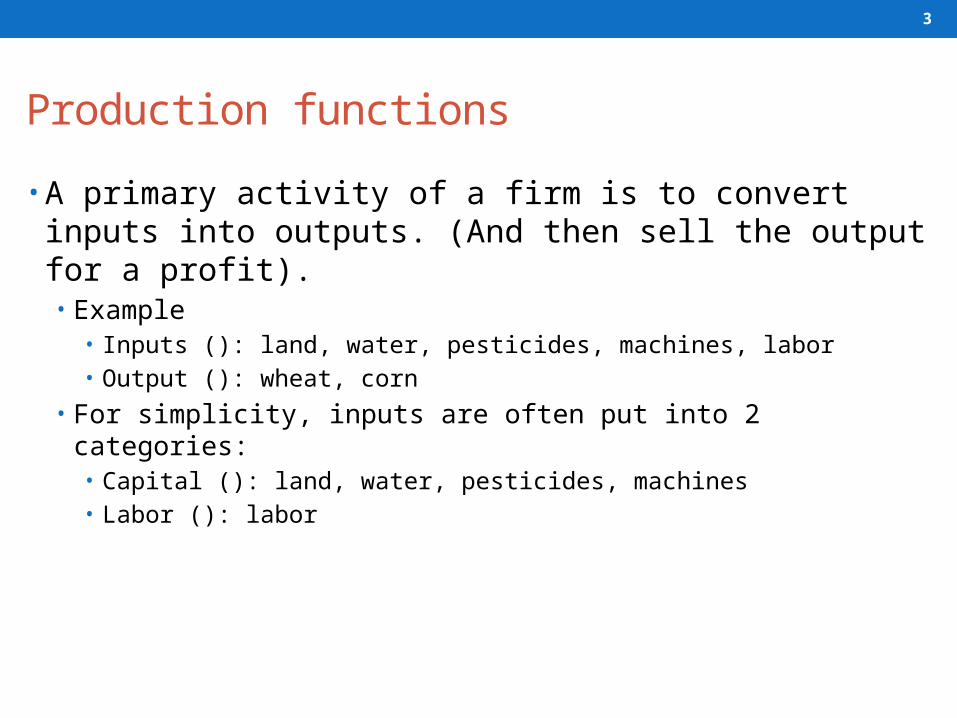
• A primary activity of a firm is to convert inputs into outputs. (And then sell the output for a profit).• Example

• Inputs (): land, water, pesticides, machines, labor• Output (): wheat, corn

• For simplicity, inputs are often put into 2 categories:• Capital (): land, water, pesticides, machines• Labor (): labor

3

Production function

• Economists represent the process of converting inputs to outputs with a production function of the form:

• is the output• are inputs• is the function that transforms inputs to outputs

4

Productive efficiency

• There are many ways to produce bushels.• Little water, much water conservation technology• Much water, little water conservation

• All possible combinations of inputs to outputs are represented by the production function

• We assume that firms are efficient in production• The production function provides the maximum amount of output that

can be produced for a given set of inputs

5

Properties of production functions

• is defined only for • are non-negative

• Straightforward – negative inputs don’t make sense

• is a single-valued function• is continuous and differentiable

6

is a single-valued function

• Remember, gives us the maximum output for a given set of inputs.

• A single-valued function means that for any given set of inputs, there can only be one level of output

7

y2

x1

y1

Can’t have this.If yields maximum for a given level , then does not make sense.

is continuous and differentiable

• We rule out these possibilities:

8

We use the notation to denote that the function is times continuously differentiable over a given region.

We usually assume is at least twice differentiable: .

Not continuous C o n t i n u o u s b u tn o t d i ff er e n ti a b l e .

Physical product relationships(2 inputs)

• Total product

• Average product

• Marginal product

9

1 2( , )TP y f x x

1 2( , )i

i i

y f x xAP

x x

1 2( , )i ii

yMP f x x

x

Total product

• Same as production function• To draw this in 2 dimensions, hold constant at (e.g. a fixed

amount of land)

10

Suppose we vary .How would we illustrate this?

1 2( , )TP y f x x

y

x1

f(x1 | x20)

Total product: Change

11

y

x1

f(x1 | x21)

f(x1 | x20)

0 12 2x x

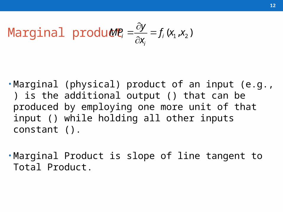
Marginal product

• Marginal (physical) product of an input (e.g., ) is the additional output () that can be produced by employing one more unit of that input () while holding all other inputs constant ().

• Marginal Product is slope of line tangent to Total Product.

12

1 2( , )i ii

yMP f x x

x

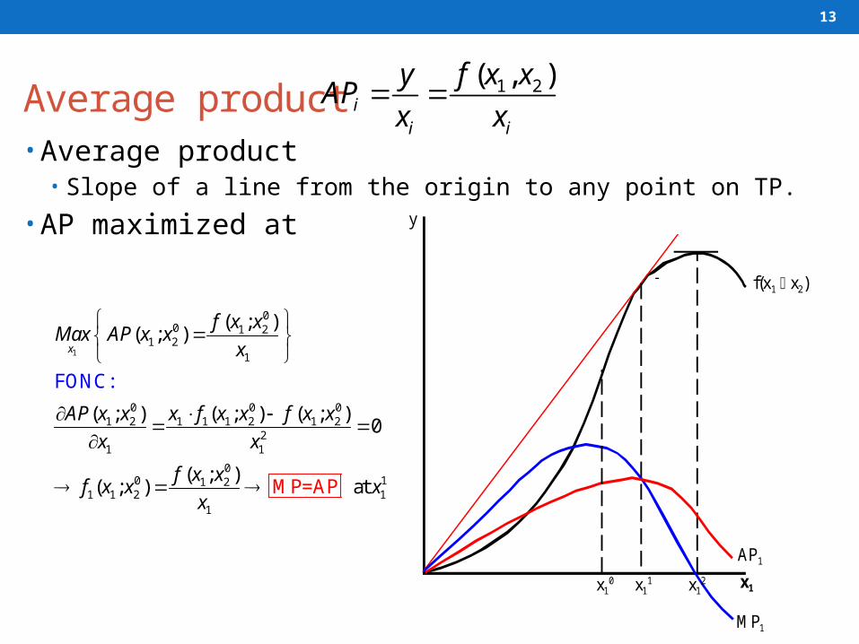
Average product• Average product

• Slope of a line from the origin to any point on TP.

• AP maximized at

13

1 2( , )i

i i

y f x xAP

x x

y

f(x1 x2)

AP1

MP1

x10 x1

1 x12 x1

1

00 1 2

1 21

0 0 01 2 1 1 1 2 1 2

21 1

00 11 2

1 1 2 11

MP=A

( ; )( ; )

( ; ) ( ; ) ( ; )0

( ; )( ; )

FON :

P

C

at

x

f x xMax AP x x

x

AP x x x f x x f x x

x x

f x xf x x x

x

Relationship between TP, AP & MP

14

Average product Max at

Marginal product Max at inflection point MP equals AP at Max

AP () at max TP ()

y

f(x1 x2)

AP1

MP1

x10 x1

1 x12 x1

Shape of production functionWhat should a production fctn. look like?• Positive marginal productivity

• Adding another unit of input will increase output

• Don’t bother adding more inputs if it’s only going to decrease output.

15

1 2( , ) 0i ii

yMP f x x

x

“The more the merrier…”

y

x1

f(x1 | x20)

2

1 22, 0( )i

iii i

MP yf x x

x x

Diminishing marginal productivity Because other inputs are held

constant, eventually the ability of an additional unit of input to generate additional output will begin to deteriorate.

“Too many cooks spoil the broth…”

We will be revisiting these conditions. Now let’s look at the production fctn in 3-D.

The Production Surface

16

1 2( , )TP y f x x

x2

y

x1

x20

Horizontal “slices” are isoquants

01 2( , )f x x y

Vertical “slices” are the 2-D TP graphs

01 2( , )y f x x

Isoquants or Level Curves

• An isoquant is a “horizontal slice” of the production function• Definition: All possible

minimum input combinations that will produce a given level of output.

• Consider the isoquants to be a view of the production surface from above.

17

x2

y

x1

a

b

x20

f(x1x2) = y0

x10

y0

y0y0

x2

x1

x20

x10

a

b

y2

y1

y0

When we hold x2 constant at x2

0, we get a 2-D total product curve.

When we hold y constant at y0, we get a 2-D isoquant.

Slope of isoquants:Rate of technical substitution (RTS)• Marginal rate of technical

substitution (RTS or MRS or MRTS) • Shows the rate at which one input

() can be substituted for another input (), while holding output constant () along an isoquant.

• RTS is the slope of the isoquant evaluated at a particular point

18

x2

x1

x20

x10

a y2

y1

y0

2

1

RTSdx

dx

Shape of isoquants:Derive RTS• The equation represents one equation in two unknowns:

and .• We can solve for one unknown in terms of the other:

• For any , the function gives us the value of such that the result will always be .

• Substitute into :

19

Shape of isoquants: Derive RTS• Slope of isoquant is:

• From last slide:

• Differentiate identity wrt :

20

x2

x1

x20

x10

a y2

y1

y0

01 2 1 1 1 2 1 2

1 1 2 1 1

( , ( )) ( , ( ))f x x x dx f x x x dx y

x dx x dx x

2 1

1 2

21 2

1

0 is the slope of the isoquant (RTS0 )dx dx

x xf f

d

f

d f

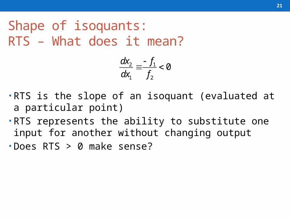
Shape of isoquants: RTS – What does it mean?

• RTS is the slope of an isoquant (evaluated at a particular point)

• RTS represents the ability to substitute one input for another without changing output

• Does RTS > 0 make sense?

21

2 1

1 2

0dx f

dx f

Shape of isoquants: What if RTS > 0 ?

• Use of beyond a (such as to b) would require more to produce • Not rational

• So…for a production function to make economic sense, RTS<0

22

x2

x1

y0

ba

y2

y1

Ridge Lines: definearea of rationalproduction

2 1

1 2

0dx f

dx f

Intuition: If both marginal products are positive, then more of both inputs (e.g. moving from a to b) must yield an increase in output, not same output.

Shape of isoquants:Diminishing RTS• Diminishing RTS:

• Intuition: To get the same with less and less , you should have to use more and more .

• Isoquants are convex• Slope from a c gets less

negative

23

x2

0 x1

b

a

c

x2(x1;y0)

dx2 / dx1

222

121

Properties of isoquants:

00 andd xx

x dx

d

d

Read Silb §3.5

If this were <0, then firms would only use one input. If the marginal benefits of x1 increased as x1 increased, why use x2?

We assert convexity because it’s the only assertion consistent with using multiple inputs.

Recall

24

1 21 2 2

1 11 12 1 11 1 11 11

2 12 22

1 22 2

2 1 11 12 1 22 1 2 12 2 11

2 12 22

bordered Hessian: 2 bordered principal minors

00

0 0

0

2 0

f ff

BH f f f BH f f ff f

f f f

f f

BH f f f f f f f f f f

f f f

1 2

21 1

2 22 1 22 1 2 12 2 11

( , ) is quasi-concave if:

0 Which is consistent with positive MP

2 0 Let's make some sense of this condition...

f x x

BH f

BH f f f f f f f

Recall: A negative definite BH is a sufficient condition for quasi-concavity

25

Express in terms of partial derivatives of

2 1 1 2 1

1 2 1 2 1

From before:

( , ( ))0

( , ( ))

dx f x x x

dx f x x x

22

1221 1

dxddxd x

dx dx

2

22 1 1 2 1 1 2 1 2 12 2

1 1 1 2

1( , ( )) ( , ( ))

d xf f x x x f f x x x

dx x x f

2 22 11 12 1 21 22 2

1 1 2

1dx dxf f f f f f

dx dx f

1 2

2 2

1

1 1

1 1

( , ( ))( , ( ))x xx

ff

x

xx

dx

d

26

22 2 2

2 11 12 1 21 222 21 1 1 2

1d x dx dxf f f f f f

dx dx dx f

2 112 21

1 2

22 1 1

2 11 12 1 12 222 21 2 2 2

Using , and :

1

dx ff f

dx f

d x f ff f f f f f

dx f f f

21 22

2 11 1 12 22 2

12

f ff f f f

f f

22 22

2 11 1 2 12?

1 222 31 2

12 0

d xf f f f f ff

dx f

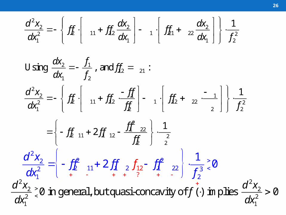
2 2

2 22 21 1

0 in general, but quasi-concavity of ( ) implies 0d x d x

fdx dx

Convexity of isoquants

• Quasi-concavity of the production function and convex isoquants are consistent.• If the isoquants are convex (a sufficient condition), then the production

function will be quasi-concave.• OR…• If we want convex isoquants, we need a quasi-concave production

function.

• Remember that a strictly concave production function (required for profit max problems) is also quasi-concave

27

22 22

2 11 1 2 1 22 312?

21 2

12 0

d xf f f f f f

dx ff

Recap…• Desirable properties for a production function:

• Positive marginal product • Diminishing marginal product • Isoquants should have

• Negative rate of technical substitution • Diminishing RTS

28

22 22

2 11 1 2 1 22 312?

21 2

12 0

d xf f f f f f

dx ff

Diminishing marginal productivity is not even necessary for convex isoquants: Convexity how marginal evaluations change holding output

constant. Diminishing marginal product refers to changes in total output

changing levels of output.