8

CHAPTER 2. GRAIN TEXTURE

INTRODUCTION

All clastic sediment is made up of discrete particles termed grains or clasts. Thus, any description of a clasticsediment must describe the particles, including their individual and bulk properties. Such properties collectivelydefine the texture of a sediment or sedimentary rock and include individual properties such as grain size and shapeand bulk properties such as grain size distribution, fabric (orientation and packing of particles), porosity andpermeability. These properties are important for any complete description of a sediment. In addition, because theseproperties are governed by processes that act at the time of deposition and, in some cases, after burial, they mightprovide insight into the history of a sediment. Furthermore, many of these properties will govern how a sedimentwill behave when used in a particular way, for example, as a final resting place for garbage. This chapter focuseson the concepts and terminology used to describe sediment texture and shows how texture may be used in makingbasic interpretations about the history of a sediment.

GRAIN SIZE

One might expect that the description of the size of particles that make up a clastic sediment would be thesimplest property to describe. However, most sediment is composed of particles with a variety of irregular shapesand may extend over a range of sizes. Therefore, the characterization of the size of particles within a sediment maynot be so straight forward.

Consider an irregularly-shaped pebble that is large enough to cover the palm of your hand. How might youtell someone else precisely how big this pebble is without actually showing it to them? You might decide that thepebble is “moderately large” and describe it as such but this is a rather ambiguous expression that could be easilymisunderstood by the other person. In this case we need some way of measuring the size of the pebble and thenwe need some consistent terminology to describe the size; a terminology that everyone else will use so that theywill know what is meant by an expression such as “moderately large”.

Grain Volume

There are several methods that will provide a quantitative measurement to describe the size of a particle. Theeasiest method would be to physically measure some linear dimension of a particle. This is simple enough if theparticle is a perfect sphere, it will have only one linear dimension: its diameter. However, natural particles arecommonly not very spherical and one linear dimension may not adequately describe their size. A measure of sizethat can be determined while neglecting the shape is the volume (V) of a particle. A simple way to determine thevolume of a particle is to determine its mass (m) and calculate volume from the relationship:

m = Vρ Eq. 2-1

where r is the density of the particle. The mass can be determined by weighing the particle. We might assume areasonable density of the particle, say that of quartz (2650 kgm-3), and solve for V. However, the actual density ofthe material comprising the particle may vary significantly from the assumed value.

The volume of the particle may also be determined directly by measuring the volume of fluid displaced bythe particle when it is immersed in the fluid within a graduated cylinder or beaker. This method does not requirean assumption of the density of the particle but may derive error if the particle is made up of a porous material andall of the pores do not become saturated with the fluid. We can often neglect this source of error.

In the case of particles that are perfect spheres of non-porous solid we can calculate the volume of the particlewith diameter d from:

Vd

=π 3

6Eq. 2-2

9

Linear Dimensions

Direct Measurement

As noted above, the easiest way the determine and express the size of a particle is by describing its lineardimensions. Because a sedimentary grain is rarely a perfect sphere we normally treat each grain as if it was a triaxialellipsoid (Fig. 2-1) and its linear dimensions are described in terms of the lengths of the three principle axes: the longaxis (a-axis or d

L), the intermediate axis (b-axis or d

I), and the short axis (c-axis or d

S)

To measure these lengths on a particle follow the steps below and refer to figure 2-2.

1. Determine the plane of maximum projection of the particle. This is an imaginary plane passing through the particlesuch that the intersection of the particle and the plane produces the largest possible surface area (i.e., the maximumprojection area).

2. Establish the maximum tangent rectangle for the maximum projection area. This is a rectangle that, when placedaround the maximum projection area, results in the maximum possible tangential contact with the outline of theparticle.

3. Measure the length of the a- and b-axes such that the a-axis length is the length of the long side of the maximumtangent rectangle and the b-axis length is the length of the short side of the maximum tangent rectangle.Note that the plane of maximum projection is the a-b plane of the particle.

4. Measure the c-axis length as the longest distance through the particle, perpendicular to the a-b plane.

The above procedure is used so that different workers can produce comparable results; it provides a standardfor all workers. For large particles, reportedly as small as 0.25 mm, all three axes may be measured. For larger particles,in excess of a few millimetres, callipers may be used to measure the axes. For smaller grains the axes may be measuredunder a binocular microscope. When a grain is too small to allow it to be rotated to see the short axis the long andthe intermediate axis may be measured. A common practice is to measure only d

L and different particles may be

compared only in terms of their maximum axes lengths. However, this practice may lead to considerable error,especially if the shapes of particles varies considerably.

In many studies of particle size, especially coarse particles, grain size is expressed in terms of the nominaldiameter (d

n): the diameter of a sphere having the same volume as the particle. If the three principle axes lengths

are known this expression of grain size is easily calculated by:

n L I Sd d d d= 3 Eq. 2-3

Nominal diameter is just one of a large number of expressions of linear dimension that have been used to describe

dL

dS

dI

Figure 2-1. Definition of principle axes of a sedimentary particle.

10

Maximum

Projection area

dId

L

dS

Maximum Tangent Rectangle/a-b plane

Figure 2-2. Sketch showing the method for determining the lengths of the principle axes of a particle. After Blatt,Middleton and Murray, 1980.

the size of a particle.

Sieving

Sieving is a method that is widely used to directly measure the sizes of a large number of grains (samplesrange from 40 to 75 grams) and is normally limited to particles in the range from as fine as 0.0625 mm up to as largeas 64 mm. The detailed procedure that should be followed when sieving a sediment sample is outlined in Appendix1. Again, a specific procedure has been derived so that results of different workers will be reliably comparable. Theequipment that is used world-wide for sieving includes a shaker and a series of nested, square holed screens (thescreen with the largest holes on top, down the smallest holes on the bottom). The sediment sample is passed throughthe screens, by shaking, and the weight of sediment that accumulates on each screen is weighed. Thus, theinformation obtained is not the absolute size of each grain but the frequency of grains (by weight), in a sample, thatfall between the range of sizes represented by the square holes in the screen above and in the screen on which thegrains are resting. The actual dimension of the grains that might be considered is "the largest square hole throughwhich the grains will pass". This dimension is approximately the intermediate axis length. The procedure and themeaning of grain size data will become more clear later in this chapter.

Settling Velocity

Another very useful measure of grain size is the settling velocity of a particle. A particle's settling velocity(or fall velocity) is normally defined as the terminal velocity that a particle will reach while falling through a still fluid,normally water. A particle's settling velocity (ω) is related directly to its size (d) and also to its density (ρ

s) but is

also influenced by fluid properties such the fluid density (ρ) and the viscosity (µ); for all fluids these propertiesvary with temperature.

To measure the settling velocity of a particle we may simply, but accurately, record the time that it takes tofall a known distance through a column of still fluid contained within a transparent tube (termed a settling tube).This is relatively simple if we are timing the settling rate of only one or a few grains but becomes difficult if we mustdeal with a sample from a population of grains of non-uniform size (and therefore varying settling velocity). In thiscase we must time the settling rate of large numbers of grains. A variety of types of settling tube have been devisedand these are described in several publications (see Blatt et al. 1980).

When using settling tubes a number of factors that will influence the results must be considered. First, when

11

a particle first begins to fall through the fluid it will accelerate from rest (i.e., zero velocity) to some constant (terminal)velocity. Thus, the settling velocity may be under-estimated if the distance over which the particle passes duringthe phase of acceleration is large in comparison to the total distance over which settling is timed. This can beovercome by using a tube that is long enough so that the distance over which acceleration takes place is relativelysmall. This may be a problem for relatively large particles but for less than 1 mm diameter particles of quartz-densitythe distance required to achieve terminal velocity is less than a centimetre. When dealing with samples of morethat one particle care must be taken that the grains settle independently and do not interact during passage throughthe fluid. Sample sizes will depend on the type of settling tube used and should generally be less than 10 grams.Samples that are too large may cause settling en masse so that the velocity determined will not be the velocity ofindividual grains. Also, large quantities of grains in the tube may interact directly (e.g., collide), altering the settlingrate, or indirectly by causing the fluid itself to move (i.e., cause turbulence) so that the velocity of the grains is notthat in still fluid. A further requirement of apparati for measuring settling velocity is that the tube diameter mustbe at least five time the average diameter of the particles that will pass through it. When a particle passes througha fluid it must "push" the fluid out of its path. At the tube wall the fluid is more difficult to push than it is well awayfrom the wall region due to fluid viscosity. Thus, a small ratio of tube to particle diameter may result in the passageof grains too close to the tube walls where they will be travel slower than they would through fluid that is notsignificantly influenced by wall effect.

Stokes’ Law of Settling

The relationship between grain size (e.g., diameter) and settling velocity is an interesting one that reflectsa variety of principles that will be of interest later in these notes. The relationship is relatively complex due to a numberof factors. Theoretical relationships have been developed and compared to experimental data collected by actuallymeasuring settling velocity in settling tubes. One such theoretical relationship between grain size and settlingvelocity is Stokes' Law of settling.

The derivation of Stokes' Law is simple but instructive. It is based on a simple balance of forces that acton a grain as it is falling at terminal velocity through a still fluid and the knowledge that the velocity will be affectedby grain size (d), grain density (ρ

s), fluid viscosity (µ), fluid density (ρ), and the acceleration due to gravity (g).

Consider the forces acting on the spherical particle falling through a still fluid as shown in figure 2-3. As the particlebegins its passage through the fluid three forces are involved: the gravity force (F

G), which is the weight of the

particle acting to move it downward through the fluid; a buoyant force (FB), acting to move the particle upward

through the fluid; and a drag force (FD) that retards the movement of the particle through the fluid. The gravity

and buoyant forces may easily be quantified. The gravity force is just the weight of the particle and is equal to thevolume of the particle times its density times the acceleration due to gravity:

FB

FG

FDFD

FB: Bouyant Force

FD: Drag Force

FG: Gravity Force

Figure 2-3. Forces acting on a spheri-cal particle falling through a stillfluid.

12

F gdG s=π ρ6

3 Eq. 2-4

FG acts in the downward direction, causing the particle to settle. The buoyant force acts in the opposite direction

and is simply the weight of the fluid that is displaced by the particle (i.e., the weight of fluid with a volume equalto that of the particle):

F gdB =π ρ6

3 Eq. 2-5

Because FG and F

B act in opposition the net force that acts on the particle (FG

' ) is given by:

F F F s g d g d s g dG G B' ( )= − = − = −

π ρ π ρ π ρ ρ6 6 6

3 3 3 Eq. 2-6

Clearly, when the density of the particle exceeds the density of the fluid it will settle through the fluid becauseF

G > F

B . Note that the expression on the right hand side of Eq. 2-6 is termed the submerged weight of a particle.

The drag force exerted on the settling particle is more difficult to determine. This force arises from the resistanceof the fluid to deformation due to the fluid property termed dynamic viscosity and is normally given the symbol m,and is expressed as Nsm-2. Fluids that offer a large resistance to deformation have a high viscosity (e.g. molasses)whereas fluids with low viscosity deform readily. Experiments have shown that the drag on a particle varies withthe velocity at which the particle passes through the fluid. Specifically, experiments have shown that at relativelylow settling velocities the drag force can be calculated from:

F d UD = 3π µ Eq. 2-7Stokes derived his law of settling from the two forces acting on a settling particle: the submerged weight and thedrag force. When a particle is settling at its terminal velocity no net force must be acting on it (i.e., the velocity isconstant, neither accelerating or decelerating, therefore experiencing no net force). Therefore, when a particle

reaches terminal velocity FD and FG

' must be equal in magnitude but act in opposite directions (FD acts upwards

and the submerged weight acts downwards). Thus, when a particle reaches terminal settling velocity:

F F FD G B= − Eq. 2-8Setting this equality and substituting with equations 2-6 and 2-7:

36

3π µ π ρ ρd U gds= −( ) Eq. 2-9

Because the particle is falling at its terminal velocity the velocity term in FD is the settling velocity so that U=w.

Therefore, we can solve Eq. 2-9 for ω:

ω π ρ ρπ µ

ρ ρµ

= − × =−

6

1

3 183

2

( )( )

ssgd

d

gdEq. 2-10

Thus, Stokes' Law of Settling is simply:

ωρ ρ

µ=

−( )s gd 2

18Eq. 2-11

Table 1 shows an example calculation of the settling velocity of a particle using Stokes' Law. Note that whenmaking such a calculation you must state all of the conditions (e.g., sediment and fluid density, fluid temperatureand viscosity), in many cases these conditions must be assumed. The statement of conditions is particularlyimportant because there are severe limitations to the use of Stokes' Law of Settling. These limitations are outlinedin the following paragraphs.

Stokes’ Law is reliable only for grain sizes finer than approximately 0.1 mm. Figure 2-4 shows that Stokes'Law predicts the settling velocity of quartz-density particles quite reliably up to a grain size of approximately 0.1mm, beyond which the theoretical relationship increasingly overestimates the observed settling velocity. Thisoverestimation is due to the fact that Stokes' Law only includes viscous drag on the particle. When larger grains

13

Table 2-1. Example of Stokes' Law of Settling

Consider a spherical quartz particle with a diameter of 0.1 mm, in still, distilled water.

ρs= 2650 kg/m3

ρ= 998.2 kg/m3, density of water at 20°C

µ = 1.005x10-3 N.s/m2, water at 20°C

g = 9.806 m/s2

(note that in the calculation, for consistent units, the diameter of the particle is expressed as 0.0001 m)

By Stokes’ Law the Settling, the terminal fall velocity of this particle is 8.954 x 10-3 m/s (~ 9 mm/s).

settle they travel at relatively high velocities through the fluid and eddies develop in their wake. These eddies impartan additional form of resistance that acts to further reduce their terminal settling velocity. Because Stokes' Lawneglects this additional force of resistance it predicts a larger settling velocity than that determined by actualexperiments (Fig. 2-4). Figure 2-5 shows an additional shortcoming of Stokes' Law when applied to sedimentaryparticles that settled in a fluid for which the temperature is not known. Because of the effect of temperature on fluiddensity and, especially, fluid viscosity, the settling velocity of a particle will vary over almost an order of magnitudethrough the range of temperatures that might naturally occur at the earth's surface. Thus, application of Stokes'Law to predict the settling velocity of a particle in some unknown depositional environment (and unknowntemperature) may lead to considerable error.

A further problem that arises when applying Stokes’ Law to natural sedimentary particles is that it onlyapplies to spherical particles. Grain shape can have a dramatic effect on settling velocity. In a simple case, shapecan effect the orientation of the grain as it settles thus affecting the surface drag that acts on the particle as it passesthrough the fluid. A more dramatic example is that of a platy particle (e.g., a flake of mica) which tends to drift backand forth as it settles rather than falling vertically though the fluid.

Finally, Stokes’ Law applies to particles falling through a still fluid. That is, the fluid is at rest except where

Figure 2-4. Somewhat schematic illustration showing thesettling velocities of spherical, quartz-density particles instill water at 20°C, as predicted by Stokes' Law of Settling,compared to experimentally-determined settling velocitiesof similar particles. After Leeder (1982).

1000

100

10

1

0.10.01 0.1 1.0 10

Quartz sphere diameter (mm)

Fal

l vel

ocity

(m

m s

-1 )

Sto

kes'

Law

Exper

imen

tal curve

14

it is accelerated, due to viscosity, by the passage of the particle itself. Therefore, it is unreasonable to apply Stokes’Law to the settling velocity of particles in a moving, particularly turbulent, fluid (e.g., particles in a river) where fluidforces will act to move the particle up, down and sideways.

Before leaving Stokes' Law of Settling we can return to the discussion of the expression of grain size as somelinear dimension of a particle. Sedimentologists have traditionally preferred to express grain size as some lineardimension and Stokes' Law can also be used to determine such a dimension for comparison of different sedimentaryparticles. This linear dimension of a particle is termed Stokes' Diameter (d

s; also termed settling diameter) of a particle

and is defined as the diameter of a sphere with the same settling velocity as the particle. We can determine theStokes' Diameter of a particle by measuring its settling velocity in still water and by solving for particle diameterin Eq. 2-11. Thus, if the settling velocity of a particle is known, Stokes' Diameter may be calculated from:

dgs

s

=−

18µωρ ρ( ) Eq. 2-12

Grade Scales

In the introduction to this chapter we posed the question of how do we verbally describe the size of a particlein such a manner that would be understood by others. A grade scale provides such a standard for verballyexpressing and quantitatively describing grain size. Any good grade scale should:

(i) Define ranges or classes of grain size (grade is the size of particles between two points on a scale. e.g., “veryfine sand”, is a grade between maximum and minimum size limits),

and

(ii) Proportion the grade limits so that they reflect the significance of the differences between grades. For example,the change in size from 1 mm to 2 mm diameter sand is an increase of 100%, however, the change in size from 10 mmto 11 mm is on the order of 10%. Therefore, a grade scale in which grade limits vary by 1 mm would not be useful.

The most widely-used grade scale is the Udden-Wentworth Grade Scale (Fig. 2-6). Note that most of the grade

100

10

10 20 40 60 80 100

Temperature (˚C)

Sto

kes'

Set

tling

Vel

ocity

(m

m s

-1)

Stokes' settling velocity:0.1 mm quartz grain in still water

Figure 2-5. Effect of fluid temperature on set-tling velocity. Curve shows settling velocitycalculated using Stokes' Law of Settling appliedto a 0.1 mm diameter quartz sphere setting throughstill water.

15

Boulders

Cobbles

Pebbles

Granules

Very Coarse Sand

Coarse Sand

Medium Sand

Fine Sand

Very Fine Sand

Silt

Clay

Size(mm)

256

Size(φ)

-8

64 -6

4 -2

2 -1

1 0

0.5 +1

0.25 +2

0.125 +3

0.0625 +4

0.0039 +8

Gra

vel

San

dM

ud

Dir

ect

Mea

sure

men

t

Sie

vin

g

Set

tlin

g T

ub

e

Bin

ocu

lar

Mic

rosc

op

e

Measurement techniques

Sed

igra

ph

Figure 2-6. The Udden-Wentworth Grade Scale defining the range of sediment sizes per size class and the verbalexpression used to describe each size class. Also shown are the techniques that may be used to measure grain size andthe grain size limits over which they should be used. After Pettijohn, Potter and Siever, 1973.

boundaries increase by a factor of 2, reflecting significant changes in grain size. Also, the scale defines limits forthe verbal expression of grain size. "Very fine sand" is sand which ranges in size from 0.0625 mm to 0.125 mm

Krumbein (1934) introduced a logarithmic transformation of the scale which converts the boundariesbetween grades to whole numbers. This scale is known as the Phi Scale, it’s values being denoted by the Greekletter phi (φ), where:

φ = -log2 d(mm) Eq. 2-13

where d(mm) is just the grain size expressed in millimetres. For example:

-log2 1(mm) = 0 φ

-log2 1/4(mm) = 2 φ

-log2 4(mm) = -2 φ

φ was later redefined:φ = -log

2 d/d

o2-14

where d is the size in millimetres and do is a standard size of 1 mm; division by 1 mm does not alter the value of φ

but makes it dimensionless.

With a hand calculator the conversion from φ to mm and from mm to φ is as follows:

φ → mm d(mm) = 2-φ

mm → φ φ = -( log10

d)/log10

2

Note that it is traditional among sedimentologists to plot grain size on a phi scale with decreasing grain size to theright as shown in figure 2-7.

16

Frequency

increasing grain size decreasing grain size

0 1 2 3 4-1-2-3-4

Grain Size (φ)

Displaying Grain Size Data

Most data describing the grain size distribution of a bulk sample of sediment are in the form given in Table2-2 which shows the frequency distribution (in terms of weight) of sediment per size class (here grain size classesare at 0.5 φ intervals). In the case of data derived from sieving a sediment sample each value in column 2 is the weight,in grams, of sediment accumulated on the sieve with openings indicated by the grain size class (column 1). Tofacilitate comparison of samples of different weight the frequency distribution is more commonly calculated as aweight expressed as a percentage of the total weight of the sample (column 3). Column 4 is the cumulative weight(%) derived by incrementally summing the values in column 3. Several ways in which such data may be plottedto graphically display the grain size distribution of a sample are shown in figure 2-8.

Histograms, such as figure 2-8A, are valuable because they readily show the relative proportions of eachsize class and the modal class of the distribution (the size class with the largest frequency). Also shown in figure2-8A is the frequency curve for the data, a smoothed version of the histogram formed by joining the midpoints ofeach size class on the histogram. Note that there are two vertical scales in this example, one shows the absoluteweight per size class and the other shows the weight expressed as a percentage of the total sample weight per sizeclass. In this case the data are normally distributed and the frequency curve forms a bell-shape which is symmetricalabout its highest point. Figures 2-8B and C are cumulative frequency curves for the data in Table 2-2, column 4.

Figure 2-7. Conventional phi scale showing grain sizeincreasing to the left and decreasing to the right.

Table 2-2. Example of grain size data produced by sieving (note these data are plotted in Figure 2-8).

1. Grain Size 2. Weight 3. Weight 4. Cumulative WeightClass (φ) (grams) (%) (%)

-0.5 0.40 1.3 1.30 1.42 4.6 5.9.5 2.76 8.9 14.81 4.92 15.9 30.71.5 5.96 19.3 502 5.96 19.3 69.32.5 4.92 15.9 85.23 2.76 8.9 94.13.5 1.42 4.6 98.74 0.40 1.3 100.0Total 30.92 100

17

-1 0 1 2 3 40

1

2

3

4

5

6

0

5

10

15

20

Indi

vidu

al W

eigh

t (gr

ams)

Individual Weight (%

)

Histogram

Frequencycurve

Grain size (φ)

A. Histogram and frequency curve

-1 0 1 2 3 4

Grain size (φ)

Cum

ulat

ive

Wei

ght (

%)

0

10

20

30

40

50

60

70

80

90

100

B. Cumulative frequency curveon an arithmetic scale

-1 0 1 2 3 4

Grain size (φ)

0.01

1

99.99

99

50

80

2010

90

Cum

ulat

ive

Wei

ght (

%)

C. Cumulative frequency curve on a probability scale

Figure 2-8. Various ways in which grain size data (Table 2-2) may be graphically displayed.

Figure 2-9. A. Illustration showing how a percentile may be determined from a cumulative frequency curve. B. Schematicillustration showing the cumulative frequency curve of a sediment population composed of three subpopulations. Note thatboth graphs are plotted on probability scales.

-1 0 1 2 3 4

Grain size (φ)

0.01

1

99.99

99

50

80

2010

90

Cum

ulat

ive

Wei

ght (

%)

A. Definition of Percentile

-1 0 1 2 3 4

Grain size (φ)

0.01

1

99.99

99

50

80

2010

90

Cum

ulat

ive

Wei

ght (

%)

B. Grain size population of three normallydistributed subpopulations

φ20 = 0.86 φ

One of the major benefits of plotting grain size data as cumulative frequency curves is that the data form a uniquecurve for each possible grain size distribution. Such curves may be plotted on graphs with arithmetic axes (Fig.2-8B) or more commonly on graphs with a vertical “probability” scale which expands the low and high ends of thescale and compresses the middle of the scale (Fig. 2-8C). One advantage of plotting such data on a probability scale(Fig. 2-8C) is that normally-distributed data plot as a straight line. Moreover, if the sediment sample is made up ofseveral normally-distributed subpopulations its’ cumulative frequency curve, plotted on a probability scale, willform straight-line segments, each corresponding to a subpopulation of the total sediment (Fig. 2-9B). Anotherbenefit of constructing cumulative frequency curves is that percentiles can be taken directly off the graph (Fig.2-9A). The nth percentile (denoted φ

n in this context) is the grain size, in units of φ, which is finer that n % of the

total sample. In figure 2-9A φ20

is shown to be 0.86 φfor the hypothetical sample. Several descriptive measuresof grain size distributions have been based on percentiles taken directly from cumulative frequency curves (seeTable 2-3).

Describing Grain Size Distributions

18

There are several different properties of grain size distributions that may be described both qualitatively andquantitatively. The most common of these are outlined below. Table 2-3 summarizes some widely-used formulaefor computing the descriptive measures of grain size distributions. Note that the graphic method uses percentilestaken directly from cumulative frequency curves (see Fig. 2-10)

Median (Md)

This is the mid-point of the distribution (i.e., the grain size for which 50% of the sample is finer and 50% is coarser).

Mean (M)

The mean is the arithmetic average size of the distribution (Fig. 2-11). For perfectly symmetrical normal

Table 2-3. Descriptive measures of sediment size distribution.

Measure Graphic Method Moment Method(Folk and Ward, 1957) (after Boggs, 1987)

Median (Md) φ50 —

Mean (M)φ φ φ16 50 84

3

+ + fm∑100

Standard Deviation (s)φ φ φ φ84 16 95 5

4 6 6

−+

−.

f m M( )−∑ 2

100

Skewness (Sk)φ φ φ

φ φφ φ φ

φ φ84 16 50

84 16

95 5 50

95 5

2

2

2

2

+ −−

++ −

−( ) ( )

f m M( )−∑ 3

3100σ

Kurtosis (K)φ φφ φ

95 5

75 252 44

−−. ( )

f m M( )−∑ 4

4100σ

where: φn is the nth percentile of the size distribution taken from the cumulative frequency curve;

φ is the weight of sediment per size class as a percentage of the total sample weight;m is the midpoint of the size class.

0.01

0.050.10.20.5

12

5

10

20

3040506070

80

90

95

9899

99.899.9

99.99

-3 -2 -1 0 1 2 3 4

Cu

mu

lati

ve F

req

uen

cy (

%)

Grain Size ( )φ

φ16 φ

50φ84

Folk and Ward Formula for Graphic Mean:

+ + M z =

3

from the cumulative frequency curve:

φ16 = -0.59 φ

φ50 = 0.35 φ

φ84 = 1.27 φ

∴

M z =−0.59 + 0.35 + 1.27

3

Example calculation of grain size statistics by the graphical method

= .34φ16 φ50 φ84

φ

Figure 2-10. Example of calculating the mean of asize distribution by the graphical method.

19

distributions the mean is equal to the median. Note that the true mean cannot be determined from data collectedby sieving but can be approximated by the formulae shown in Table 2-3.

Sorting or Dispersion Coefficient (σσσσσ)

This is the standard deviation of the distribution and reflects the variation in grain sizes that make up asediment. Its’ calculated value relates to the mean of the distribution as illustrated in figure 2-11. This figure showsthat 68% of the distribution (i.e., 68% of a sediment sample, by weight) has a grain size that is within ±1σ of the mean.For example, if the mean of the distribution is 1.45 φ and the sorting coefficient is 0.30 φ, then 68% of the samplelies in the size range from 1.15 φ to 1.75 φ. Therefore, the larger the sorting coefficient the greater the range of grainsizes that make up the sediment. A sediment that consists of only a small range of grain sizes (i.e., σ is small) is saidto be well sorted whereas a sediment made up of a wide range of grain sizes (i.e., σ is large) is said to be poorly sorted.Figure 2-12 very schematically illustrates the appearance of various degrees of sorting. Descriptive grades of sortingare:

0 < σ < 0.35φ very well sorted0.35 < σ < 0.5φ well sorted0.5 < σ < 0.71φ moderately well sorted0.71 < σ < 1.00φ moderately sorted1.00 < σ < 2.00φ poorly sorted2.00 < σ < 4.00φ very poorly sortedσ > 4.00φ extremely poorly sorted

Figure 2-11. Relationship between sorting coefficient(standard deviation) and mean of a normal distribution.After Friedman and Sanders (1978).

Figure 2-12. Schematic illustration of vari-ous degrees of sorting. After Anstey andChase, 1974.

Indi

vidu

al w

eigh

t (%

)

Grain size (φ) finecoarse1σ

68%

1σ M

Very well sorted Well sorted

Moderately sorted Poorly sorted

20

Skewness (Sk)

Skewness is a measure of the symmetry of the grain size distribution about the mean; it has a maximumpossible value of +1 and a minimum possible value of -1. A of skewness that is close to zero indicates that thedistribution is very symmetrical and the mean is equal, or nearly so, to the median and both fall within the modalclass. A positive value of skewness indicates that the distribution has a larger proportion of fine grains than if thedistribution were symmetrical. Conversely, if the value of skewness is negative the distribution is enriched in coarsegrains. Figure 2-13 schematically shows the various “types” of skewness.

Descriptive terms for skewness are: Sk >+0.3 strongly fine skewed+0.1 < Sk < +0.3 fine skewed-0.1 < Sk < +0.1 near symmetrical-0.3 < Sk < -0.1 coarse skewedSk < -0.3 strongly coarse skewed

Kurtosis (K)

Kurtosis is a measure of the degree of “peakedness” of the distribution. Oddly enough, while it is one ofthe common descriptive parameters for grain size distributions it is widely thought to be essentially of no value (seejust about any textbook). None-the-less, it has become somewhat of a tradition. Figure 2-14 schematically showsdifferences between the three types of kurtosis that a distribution might display: leptokurtic (sharp-peaked; K >1), mesokurtic (normal; K = 1), and platykurtic (flat-peaked; K < 1).

Paleoenvironmental Implications of Grain Size

For many years it was thought (and hoped) that the characteristics of grain size distributions were governedlargely by processes within the depositional environment. Therefore, properties like mean size, sorting, skewness,etc., would cumulatively reflect these processes and provide a basis for interpreting ancient depositionalenvironments. This was a powerful reason for sedimentologists to study grain size distributions and many did just

Indi

vidu

al w

eigh

t (%

)Grain size (φ)

finecoarse

Mo = M = Md Sk = 0In

divi

dual

wei

ght (

%)

Grain size (φ)finecoarse

Mo

Md

M

Excess fineparticles

Indi

vidu

al w

eigh

t (%

)

Grain size (φ)finecoarse

Sk > 0

Indi

vidu

al w

eigh

t (%

)Grain size (φ)

finecoarse

Sk < 0MoMd

M

Excess coarseparticles

Figure 2-13. Schematic illustration of the various types of skewness. Note that dashed lines indicate the symmetricaldistribution for comparison with fine and coarse skewed frequency curves. M is mean, Md is median and Mo is mode.AfterFriedman and Sanders (1978).

21

Indi

vidu

al w

eigh

t (%

)

Grain size (φ)finecoarse

Leptokurtic

Mesokurtic

Platykurtic

Figure 2-14. Examples of different types of kurtosis. AfterBlatt, Middleton and Murray (1980).

+2.50

+2.00

+1.50

+1.00

+0.50

0.00

-0.50

-1.00

-1.50

-2.00

-2.50

-3.00

-3.500.10 0.20 0.30 0.40 0.50 0.60 0.70 0.80 0.90 1.00 1.10 1.20 1.30 1.40

STANDARD DEVIATION (sorting)

SK

EW

NE

SS

River sandBeach sand (ocean)Beach sand (lake)

that throughout much of the 20th century. There was limited success. Results of one successful study are shownin figure 2-15 and suggest that beach and river sediment can be distinguished on the basis of a simple plot ofskewness versus standard deviation (sorting coefficient). This figure shows relatively good separation of beachsands (generally coarse skewed and better sorted) and river sands (fine-skewed and somewhat less well sorted).The difference arises because rivers are capable of transporting a relatively wide range of grains sizes, particularlya large proportion of fine sediment that is transported in suspension when the rivers are in flood. The river deposits,therefore, tend to be relatively poorly sorted and enriched in fine grained sand (i.e., fine skewed). In contrast,beaches experience the ongoing swash and backwash of waves running up and down the beach slope. These veryshallow flows tend to segregate the sediment very efficiently, particularly in washing fine-grained material out tothe sea or lake. Thus, beach deposits are rather well-sorted and somewhat enriched in the coarser grain size (i.e.,coarse skewed)

The success of this approach to paleoenvironmental interpretation has been very limited. The main problemis that factors other than processes in the depositional environment have a profound affect on grain sizedistributions. For example, the size distribution of the constituents of the source rock (i.e., the rock that weathersto produce the sediment) may be reflected in the size distribution of the deposited sediment. If a river is transportingsand that has weathered out of a pre-existing rock formed of sand that was laid down millions of years ago on abeach, the river sediment will continue to display a size distribution which is inherited form the beach deposits.

Figure 2-15. Plot of skewness versus sortingcoefficient based on samples of river and beachsands. After Friedman, 1967.

22

Thus, if we plotted that river's sediment on figure 2-15 we would mistakenly interpret the deposit as that of a beach.

Why measure grain size?

There are many reasons to quantitatively describe grain size distributions. Some of these are:

1. Grain size is important to determining the strength of currents that transported the sediment. Therefore, we needa precise measurement of size to quantitatively interpret paleohydraulic conditions.

2. Sorting reflects the ability of the transport mechanism to segregate grains by size.

3. Skewness reflects the ability of the transport mechanism to selectively remove coarse or fine grain sizes.

4. It appears that grain size distributions like that shown in figure 2-9B have very specific interpretations in termsof how the sediment moved while it was in transport. (More on points 1 through 4 later in Chapter 4.)

5. We need basic descriptors of sediment size to allow us to communicate with others.

6. Grain size and various properties of its distribution are important in determining a sediment's porosity andpermeability.

GRAIN SHAPE

Grain shape is another fundamental property of particles and one that may provide important informationabout the history of a sediment. Like grain size, shape may be expressed in several different ways, including:Roundness, a measure of the sharpness of the corners of a grain; Sphericity, a measure of the degree of similaritybetween a grain and a perfect sphere; Form, an expression of the overall appearance of a particle. Methods ofquantitatively describing these three expressions of grain shape are outlined below.

Roundness

The roundness of a particle refers to the degree of rounding (or angularity) of the edges of a particle. Ofthe three shape properties it is the most difficult to quantify.

Wadell’s Roundness (Rw)

Wadell (1932) introduced this method of determining particle roundness; it is the most accurate method butit involves the greatest effort and time. R

w is defined as the ratio of the average radii of curvature of the corners

of a grain (Σr/N; N is the number of corners) to the radius of the largest inscribed circle within the particle (R;Fig. 2-16). The maximum possible value of R

w is 1 when the particle has no measurable corners (i.e., R = r). Thus,

Rr

NRW = ∑ Eq. 2-15

Dobkins and Folk Roundness (RF)

Dobkins and Folk (1970) introduced a less tedious (and less accurate) method of calculating roundness(symbolized as R

F here) that is defined as the ratio of the radius of curvature of the particle's sharpest corner (r)

to the radius of the largest inscribed circle (R). Thus,

Rr

RF = Eq. 2-16

once again, RF approaches a value of 1 for perfectly rounded grains (i.e., no sharp corners).

Powers’ visual comparison chart

The easiest way to determine the roundness of a particle is by visual comparison with standard forms. Powers

23

Very angular Angular Sub-angular Sub-rounded Rounded Well-rounded21 3 4 5 6ρ

Rw .17 .25 .35 .49 .70 1

Figure 2-17. Powers’ (1953) visual comparison chart for grain roundness with appropriate terms for describing shape classesdefined by R

w and ρ.

R

rr

rr

rr

r

r

Grain outline

Figure 2-16 Wadell Roundness (see Eq. 2-15; after Boggs, 1967).

(1953) provided what has become the most widely used chart of grain roundness (Fig. 2-17) and is a basis for termsdescribing roundness. Note that each box in figure 2-17 shows a particular roundness class and the appropriateterm to describe each class. Also shown are values of R

w and ρ (a logarithmic transformation of R

w to whole numbers)

that quantitatively define the limits of each roundness class.

Sphericity

Various measures of the degree to which a particle resembles a sphere (i.e., its sphericity) have been devised.Sphericity not only describes one aspect of the shape of a particle but it may also be useful to understanding otherproperties of the particle such as its settling velocity. Remember, Stoke’s Law of Settling applies accurately onlyto spherical particles (less that 0.1 mm in diameter) and its error increases as the shape of the particle deviates fromthat of a true sphere. Therefore, a measure of particle sphericity provides a means of quantitatively determininghow well Stokes’ Law will predict a particles’ settling velocity. Note that sphericity is normally given the symbol“ψ”, the lower case Greek letter psi.

Wadell’s Sphericity (ψψψψψ)

Wadell (1932) defined sphericity as the ratio of the diameter of a sphere with volume equal to that of theparticle to the diameter of the sphere which will circumscribe the particle. Wadell’s measure of sphericity maytake the form:

ψ =V

VS

C

3 Eq. 2-17

where VS is the volume of the sphere with volume equal to that of the particle and V

C is the volume of the

circumscribing sphere. In this form VS may be determined by measuring the volume of water displaced by the particle

24

and VC may be calculated from the formula for the volume of a sphere taking the maximum axis length of the particle

(dL) to be the diameter of the circumscribing sphere:

V dC L=π6

3 Eq. 2-18

VC may also be calculated for a particle with shaped approximately like a triaxial ellipsoid (Fig. 2-1) by:

V d d dS L I S=π6

Eq. 2-19

Substituting these expressions for Eqs. 2-18 and 2-19 into Eq. 2-17 yields:

ψ =d d

dI s

L2

3 Eq. 2-20

As ψ approaches 1 the shape of the particle approaches that of a perfect sphere. Eq. 2-20 can be used to calculatesphericity on the basis of measurements of the principle axes of a particle.

Sneed and Folk Sphericity (yP)

Sneed and Folk (1958) argued that the volume of a particle is not as important as its maximum projection areain determining its settling velocity because drag forces act on the particle’s surface. Therefore, any measure ofparticle sphericity must be reflect the maximum projection area of a particle. They defined maximum projectionsphericity (ψ

P) as the ratio of the maximum projection area of a sphere with volume equal to that of the particle

to the maximum projection area of the particle. ψP may be calculated from the formula:

ψ PS

L I

d

d d=

23 Eq. 2-21

This is the most widely-used expression of sphericity.

Note that an expression that is very similar to ψP and based on similar reasoning, termed the Corey Shape

Factor (S.F.), is widely by used engineers to describe the overall shape of a sediment particle:

S Fd

d dS

L I

. .= Eq. 2-22

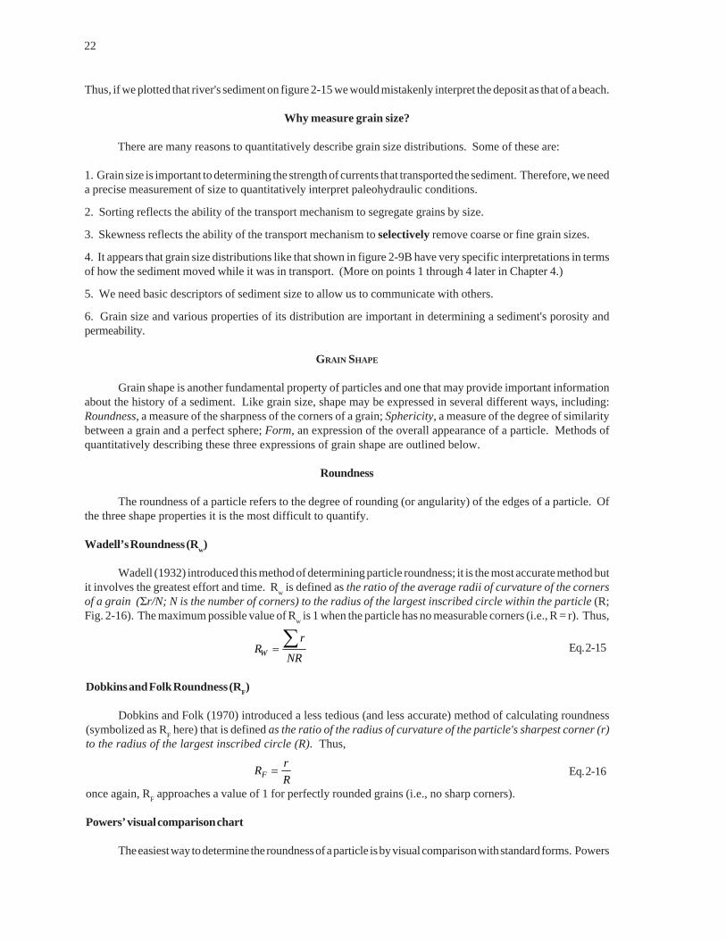
Riley Sphericity (ψR)

The main problem in calculating ψ and ψP is that both require the measurement of d

S. This is not difficult

for gravel-size particles but it becomes very impractical for sand-size sediment. Riley suggested a method ofcalculating sphericity that relies on measurements that can be taken from the two-dimensional view of a sand grainas seen through a microscope (Fig. 2-18). He defined an expression of sphericity as:

ψ Ri

c

d

d= Eq. 2-23

where dc is the diameter of a circle that circumscribes the grain and d

i is the diameter of a circle that inscribes the

grain (Fig. 2-18). Again, as ψR

approaches unity as sphericity increases.

Clast Form

There are two commonly used methods of describing the overall form of a particle, both based on variousratios of d

L, d

I, and d

S. Figure 2-19 shows the so-called Zingg diagram (after Zingg, 1935) that defines four form

fields and provides terms for clast form according to which field the axes ratios of a clast plot. The clast forms definedby the Zingg Diagram are largely independent of sphericity, except for “equant” clasts which tend to have valuesof sphericity near 1.

25

Figure 2-20 shows a second commonly-used scheme for classifying grain form that was proposed by Sneedand Folk (1958). This method classifies form into 10 possible classes and the appropriate terms for each form classis shown in figure 2-20 along with blocks that are drawn in the approximate proportions for each form field. Notealso that maximum projection sphericity may also be taken directly from this diagram and that different form classesmay have the same sphericity (i.e., form and sphericity are independent).

Significance of grain shape

Like grain size, the shape of a particle will provide some basis for making fundamental interpretations aboutthe “history” of a sediment, particularly something of the source rock of the grains and of their transport history.

Source Rock

The lithology of the source rock exerts a strong control on the form of particles, especially gravel-size clasts.Bedded source rocks (e.g., horizontally bedded limestones) tend to produce platy clasts, due to the parallel planesof weakness that the bedding produces. Massive source rocks (e.g., granites that have equal strength in alldirections) tend to produce more equant clasts. The hardness of the source rock will also control the overall shape

didC

Figure 2-18. Illustration showing the measurements required to calculatesphericity by the method proposed by Riley.

0.1

0.2

0.3

0.4

0.5

0.6

0.7

0.8

0.9

1.0

00 0.1 0.2 0.3 0.4 0.5 0.6 0.7 0.8 0.9 1.0

dd

S

I

I

L

dd

Zingg form index

OBLATE(DISK) EQUANT

BLADEDPROLATE(ROLLER)

Figure 2-19. Zingg diagram showing the classifica-tion of grain form. After Zingg (1935) and Blatt,Middleton and Murray, 1980.

26

Figure 2-20. Sneed and Folk (1958) classification ofgrain form.

0.3

0.5

0.7

0.670.33

COMPACT

COMPACT

PLATY COMPACTBLADED

COMPACT

ELONGATED

PLATY BLADED ELONGATED

VERYELONGATED

VERYBLADED

VERYPLATY

Sneed & Folk form index

dL d I

dL ds

ds

dL

0 1

1

0.20.3

0.4

0.7

0.8

0.9

ds

2d

L dI

3

ψp

=

0.5

0.6

of a particle, particularly after prolonged periods of transport (see below).

Transport

While in transport a grain will change in shape due to two major processes that may act in the transportingmedium. Interaction between grains during transport results in a change in shape and a reduction in grain size. Asgrains move along their sharp edges are lost due to chipping and grinding, increasing their roundness and sphericityand producing debris as finer sediment. Even when large clasts are partially buried in sediment beneath a currenttheir exposed surfaces are sand-blasted by particles in transport, thereby increasing their overall roundness.However, grains may be crushed during transport, producing smaller, more angular and less spherical grains.Overall, the most common outcome of transport is an increase in roundness and sphericity.

Figure 2-21 shows a plot of data derived by Humbert (1968) from experiments in which angular pebble-sizeclasts of chert (a very hard rock type) and limestone (relatively soft) were transported over several hundreds ofkilometres in a circular flume. Note that the roundness of the limestone increased more rapidly with transport thatthe chert because the softer limestone clasts are more prone to breakage (which increases rounding) than the harderchert clasts. Also, the rate of increase in rounding with increased transport distance is initially very large butbecomes smaller as the grains became rounder. This reflects the fact that an angular clast, with very sharp corners,easily becomes rounder as the fragile corners are broken off. However, a consequence of this increased roundingis that the remaining corners are more massive and difficult to break off. Therefore, as the degree of roundingincreases the rate of rounding decreases. The change in the sphericity of limestone clasts shown by the top curvein figure 2-21 is at a comparatively low rate throughout the entire distance of transport. This is because the changesthat are required to increase sphericity involve removal of a considerable amount of material from the clasts incontrast to the removal of relatively small sharp corners that results in initially dramatic increases in clast roundness.

Changes in roundness and sphericity with transport of gravel-size clasts occur at much greater rates thanfor sand-size grains (e.g., Kuenen, 1964). Because little quantitative research on changes in grain shape withtransport has been conducted on fine-grained sediment we can infer something of such changes from studies ofthe weight loss of sand with transport (increased rounding and sphericity both require weight loss). It has beenestimated that under water flows (e.g., rivers) the rate of weight loss of quartz grains finer than 2 mm is less than0.1% per 1000 km of transport. The rate increases only by a factor of two for feldspar grains. In all cases the rateof weight loss decreases sharply with decreasing grain size and becomes negligible for sizes finer than 0.05 mm.Such low rates of weight loss in very fine sediment is largely attributed to the fact that the particles spend muchof their time in transport in suspension well above the bed where interaction between particles is less frequent. In

27

air the rate of weight loss increases by a factor of 100 to 1000 times the rate in water. In water the abrasion betweenparticles that is required for such weight loss is inhibited by two factors: (1) the small submerged weight of the grainsgives them only little momentum during collisions, momentum that is required to cause damage; and (2) the viscosityof the water between colliding grains tends to dampen the collisions (further decreasing the transfer of momentum).In air, which has a considerably lower density and viscosity than water, the transfer of momentum between collidinggrains is much more effective and the resulting damage to the particles is more extensive. This (partly) explains thecommon observation that wind-blown (eolian) sands are typically much rounder and have higher values ofsphericity than sands from other environments. In ancient sediment that is clearly not of eolian origin good roundingand high sphericity are commonly interpreted to indicate that the sediment has been multi-cycled (i.e., the productof several cycles of weathering and erosion of pre-existing sedimentary rocks).

Transport may have another effect on the shape by selectively sorting clasts by shape. For example, imaginea cube and a sphere resting on the bed of a river. The sphere need only roll almost effortlessly along the bed inresponse to the fluid drag of the flowing water. In contrast, the cube must pivot over 45°, against its own weight,to roll a distance equal to its own length (if friction between the clast and the bed is large enough to inhibit it fromsliding). Thus, the sphere will more readily move under the river’s current and after a short time it will be separatedfrom the cube by a considerable distance. This processes is termed selective sorting by shape whereby easilytransported round, spherical clasts are removed from a sediment much more readily than their angular counterparts,even if both clast types have essentially the same weight. This mechanism has been suggested by studies of somemodern river gravels where there is an increase in roundness and sphericity in the downstream direction that cannotbe explained solely by abrasion (e.g., Gustavson, 1974).

There has been limited success in distinguishing ancient depositional environments on the basis of clastform. One such study showed that the deposits of gravel beaches and rivers (remember grain size) can bedistinguished on the basis of clast form. When data from these environments are plotted as in figure 2-20 the beachgravels tend to fall towards the bottom of the graph, in and about the very platy and very bladed fields, and theriver gravels tend to fall near the top of the graph, in and about the compact field. The distinction may be attributedto two causes. First, due to selective sorting of bladed clasts on the beach slope where rounded, compact clastswould be easily rolled off the beach by the backwash (water running back off the beach after a wave has rushedup its slope- the uprush is termed swash). This process would tend to enrich the beach with bladed clasts overtime. Second, the swash and backwash act to move larger, less mobile particles up and down the beach slope without

Limestone roundness

Chert roundness

Limestone sphericity

0

0.1

0.2

0.3

0.4

0.5

0.6

0.7

0.8

0.9

1.0

Rou

ndne

ss o

r S

pher

icity

0 50 100 150 200Distance of transport in a circular flume (Km)

Figure 2-21. Change in rounding (Rw) and sphericity (y

P) with transport distance in a circular flume. Based on experiments

by Humbert (1968). After Blatt, Middleton and Murray, 1980.

28

moving them entirely. This back and forth motion would result in abrasion along the basal plane of the clast andas it is periodically flipped over it would become increasingly flat (i.e., bladed or platy). These two mechanisms areabsent in rivers where currents can more efficiently roll the more compact particles along their beds.

In conclusion, grain shape is an important sediment property that, like grain size, provides hints as to theprocesses that acted to transport particles in ancient depositional environments. It is also an important variablein determining the conditions that will cause a sediment to be transported by a specific mechanisms (see chapter4). However, as with grain size, caution must be used in inferring ancient depositional conditions on the basis ofgrain shape because it is also controlled by factors other than those acting in the depositional environment.

POROSITY AND PERMEABILITY

Porosity, the proportion of void or pore space in a sediment, and permeability, which is related to how wellthe voids are connected, are important properties of any sediment or sedimentary rock. This is particularly truebecause of the possible fluids that might be contained within sedimentary deposits; e.g., water, oil and/or gas,contaminants that humans have added to the earth surface. This section defines and discusses porosity andpermeability and shows how they are related.

Porosity

Any sediment contains a certain proportion of void space; that is, the proportion of the sediment that is notoccupied by particulate solids (i.e., grains). Porosity (P) is defined as the ratio of void volume (V

P) to total rock or

sediment volume (VT), expressed as a percentage of the total sediment volume. Therefore,

PV

VP

T

= ×100 Eq. 2-24

The pore volume is generally difficult to measure whereas the total volume of grains in a sediment (VG) is relatively

easy to determine (by weighing a specimen or by placing it in water and measuring the total displacement). Becausetotal volume is the sum of pore and grain volumes V

P can easily be calculated: V

p = V

T-V

G. Substituting for V

P in

Eq. 2-24, porosity is most commonly defined as:

PV V

VT G

T

=−

×100 Eq. 2-25

Porosity in natural sediment varies from 0 to approximately 70% due to a number of factors.

What Controls Porosity?

Packing Density

There are a variety of ways that grains may be arranged in a sediment and the spacing of the particles, referredto as the packing density, exerts a strong control on porosity. This may be very simply illustrated by the mannerin which perfect spheres of equal size may be packed (Fig. 2-22). This figure shows the two-dimensional view ofspheres resting with cubic and rhombohedral packing. In the case of cubic packing the grains are stacked directlyon top of and beside each other and the pore space is relatively large (48% porosity). In contrast, with rhombohedralpacking each grain rests in the space between the subjacent grains so that the grains fill more of the space and theporosity is lower (26%). These two styles of packing produce the theoretical maximum (cubic) and minimum(rhombohedral) porosities of any sediment composed of perfectly spherical particles of equal size. In nature,particles may be arranged in styles intermediate to these two end-members and their porosities will also be of anintermediate value (i.e., between 26 and 48%). The rate of deposition of a sediment exerts considerable control overgrain packing. Rapidly deposited sands tend to have a more open framework (like cubic packing) whereas slowrates of deposition often lead to tighter packing and therefore lower porosity.

Natural sediment is rarely composed of spheres so that porosity varies over a wider range than predictedabove. Porosity varies particularly with grain shape due to the differences in packing density that may be achievedby non-spherical grains. Figure 2-23 shows how much greater porosity may vary when the particles are non-

29

spherical. In nature, angular grains tend to support a looser packing arrangement (with larger porosity) than roundedgrains.

Grain Size

By itself, grain size has no direct effect on the porosity of sediment. For example, for a sediment composedof equant spheres with cubic packing it can be shown that Eq. 2-25 reduces to

P = − ×( )16

100π

Eq. 2-26

and is, therefore, constant (P = 48%) and clearly independent of grain size.

Indirectly grain size may have some influence on porosity. For example, packing of a sediment tends toincrease with the settling velocity of the particles. When relatively larger particles, with high settling velocities,impact on a substrate they tend to jostle the previously-deposited grains into tighter packing (with lower porosity).

Several studies have shown various relationships between grain size and porosity that could be explainedin terms of other factors. In unconsolidated sands porosity tends to increase as grain size decreases. This is becausethe finer sand tends to be more angular than coarse sand and, therefore, will support a more open packing. Insandstones the opposite trend has been recognized: porosity tends to increase with increasing grain size. Thisoutcome is due to the greater tendency of fine sand to lose volume when compacted upon burial (see below)compared to the lower compaction of coarse sand. Thus, the conflicting apparent relationships between grain sizeand porosity are due to factors other than grain size.

Figure 2-23. Influence of particle shape on packing and porosity.

<50% Porosity 0% Porosity

B. Bivalve shellsA. Porosity of sediment of tabular particles

P>90%

Figure 2-22. End-member styles of packing of spheres of equal diameter and their associated porosities.

Cubic packing Rhombohedral packing

Increasing packing density, decreasing porosity

48% porosity 26% porosity

30

Sorting

The relationship between sorting and porosity is fairly straight-forward: as sorting becomes poorer (i.e.,the standard deviation of the grain size distribution increases) porosity decreases. This is illustrated in figure 2-24 for the case of clay-free sand. The reason for this relationship is obvious: the poorer the sorting the wider rangeof grain sizes within the sediment and the greater likelihood of finer grains filling the void spaces between largergrains. What is perhaps less obvious is the reason for the differences in the curves for fine and coarse sand (Fig.2-24). Note that the minimum porosity for fine sand is greater than the minimum porosity for coarse sand. This isbecause a poorly sorted coarse sand has an abundance of fine material to clog the large pore spaces between thecoarse grains. However, a poorly sorted fine sand which is free of clay (as in the case of the curves shown above)the poor sorting is by virtue of the presence of coarser sands that will not clog the pores of the finer sand. A similardifference in minimum sorting would not be expected if clay were available to clog the pores of the fine sand. Indeed,the presence of clays tends to significantly reduce the porosity of sediment.

Post-burial Processes

Several different processes act in conjunction to alter porosity after a sediment has been buried due tosubsequent sedimentation on the overlying depositional surface. Figure 2-25 shows the typical reduction ofporosity of sands with burial (although the forms of such curves vary) that can be explained by the processessummarized below. Note that some post-burial processes cause an increase in porosity; such porosity is referedto as secondary porosity. The expression Primary granular porosity is often used to distinguish porosity due tothe character of the sediment prior to burial from porosity due to changes after burial.

Compaction ⎯ With burial the weight of overlying sediment may force the sediment into a tighter packing, therebyreducing its porosity. Quartz sand shows little response to compaction; experiments have reduced the porosityof quartz sand by only a few percent due to rearrangement and breakage under stress. The reduction in porositywith compaction increases with increasing proportions of ductile (deformable) particles, especially clays minerals.When first deposited, some muds (composed largely of clays) have a very high porosity (in excess of 70%) butcompaction with burial under a thousand metres of sediment reduces that porosity to 5 to 10%.

Cementation ⎯ The precipitation of cements within a sediment may begin almost immediately following depositionor make take place after millions of years and relatively deep burial. The most common cements are calcite and quartzthat precipitates out of solution from saturated waters between grains and gradually fills in the previously openvoid space, potentially reducing porosity to 0%.

Clay formation ⎯ Chemical alteration of some minerals, particularly feldspars which are a common constituent of

01020304050

0 1 2 3 4

Standard deviation (φ)

Por

osity

(%

)

Decreasing sorting

fine sand

coarse sand

Figure 2-24. Schematic illustration showing the relationship between sorting and porosity in clay-free sands. Based on datafrom Nagtegaal (1978) and Beard and Weyl (1973).

31

clastic sediment, results in the formation of very fine-grained clay minerals that tend to accumulate within the porespaces between primary sediment grains. The formation of clays, therefore, may increase the total volume of therock at the expense of the pore volume, thereby reducing porosity.

Solution ⎯ Waters within and passing through sediment and sedimentary rocks may not precipitate cements. Ifthe waters are undersaturated with respect to the minerals with which they are in contact, these waters may dissolvethe sediment grains, leaving a cavity or vug where there had once been solid rock (note that the vugs can rangefrom microscopic in size to the size of caverns). Such solution increases the total void space at the expense of thetotal rock volume; i.e., it increases the porosity. The additional void space produced by solution is termed secondaryporosity. Carbonate rocks (which are relatively soluble) are particularly prone to the development of secondaryporosity by solution.

Pressure solution is a process that can cause a reduction in porosity following burial when mineral grainsbegin to dissolve at the grain contacts (Fig.2-26). Minerals under stress solution tend to dissolve more readily thanunstressed minerals. Within a sediment the weight of overlying material is transferred between particles at the pointswhere they are in contact. At the contacts the pressures can be immense and solution may occur as long as thereis fluid within the adjacent pore spaces. The tangential contacts between grains become increasingly flat as materialis removed into solution. The boundary between grains that have undergone pressure solution is said to be sutured.As the grains lose material at their contacts the pore space becomes markedly shorter and its volume is reduced.Concurrent with pressure solution insoluble material may accumulate in the pore space along with cements.Combined, the reduction of pore length and the deposition of material in the remaining space can cause a dramaticreduction in pore space. Once again, carbonate rocks are most prone to pressure solution and it has beendocumented to occur at burial depths of only a few tens of metres. Modern carbonate sediment has porositiesranging from 40 to 80% but carbonate rocks rarely have porosities larger than 15%. Much of this reduction canbe attributed to pressure solution. Siliciclastic sedimentary rocks can also undergo pressure solution but this ismuch less effective in reducing porosity than in carbonates.

Fracturing ⎯ Fracturing of any rock, sedimentary or otherwise, will lead to an increase in porosity. Such additionalporosity contributes to the secondary porosity of a rock. Fracture porosity may be especially important in rocksin which primary granular porosity is not well preserved.

Permeability (Darcy's Law)

Permeability (k) is related to the ability of a fluid (liquid or gas) to flow through any porous substance (e.g.,a sediment). It was first defined by the French hydrologist Henri Darcy in 1851. Figure 2-27 very schematicallyillustrates how permeability is defined. Darcy’s Law (Eq. 2-27) is an empirical formula that predicts the rate of flowof fluid through a sediment. It can be used to experimentally determine permeability by measuring the rate of

Figure 2-25. Illustration showing the reduction inporosity of tertiary sands in Louisiana. After Blatt,Middleton and Murray (1980).

0

1

2

3

4

5

6

Dep

th o

f bur

ial (

km)

12 16 20 24 28 32 36 40 44

Porosity (%)

32

discharge of fluid of known viscosity through a specimen under a known pressure gradient and solving for k inEq. 6-3. Note that k is just an empirical constant, that depends on conditions within the rock , but one which hasan important physical interpretation (termed permeability).

Darcy's Law: Q kA p

L=

∆µ Eq. 2-27

The terms are defined in figure 2-27.

For the sake of simplicity we will re-arrange the formula as follows:

Q

Ak

p

L= × ×

1

µ∆

Eq. 2-28

Q/A is equal to the average (apparent) velocity (V, in cm s-1) at which the fluid is being discharged from the sediment.Assuming that there is no compression of the fluid this is also the average velocity at which the fluid will pass throughthe sediment. Eq. 2-28 may be re-written:

V kp

L= × ×

1

µ∆

Eq. 2-29

Beginning with the right-hand-side of this formula, ∆/L is the pressure gradient along the distance of flow and

Decreasing porosity

Porosity reduction by pressure solution

Figure 2-26. Schematic illustration showing the reduction in porosity due to pressure.

Figure 2-27. Schematic illustration defining Darcy’s equation. See text for discussion.

A L

Q

p

µk

p∆

Darcy's Law

Q is the fluid discharge (cm3 s-1);k is permeability (darcies, cm2);A is cross-sectional area (cm2);∆p is the pressure difference (bars, g cm-2);L is distance over which the flow passes (cm);µ is the fluid viscosity (centipoises, g cm-1 s-1 x 10-1).

33

Region of low velocityand high resistance

Figure 2-28. The relationship between the cross-sec-tional area of a pathway and the relative proportion of thatcross-sectional area where fluid velocity is small due toviscous resistance along the wall of the pathway.

Figure 2-29. Definition of tortuosity. See text fordiscussion.

Pathway

L2

L1

Tortruosity = L2/L1

represents the force that is acting to push the fluid through the sediment. As the pressure gradient increases sowill the average velocity. The term 1/µ is a measure of how easily the fluid can flow through the sediment (i.e., asviscosity, a measure of fluid resistance to deformation, increases, 1/µ decreases). Therefore, as viscosity increasesthe velocity must decrease. So the velocity of a fluid passing through a sediment depends on the force appliedto that fluid and on how much the fluid will resist flow through the sediment. But we have not yet considered howthe sediment itself will influence the velocity of the fluid passing though it; that is the role of the permeability termin the Darcy’s Law. Permeability is a measure of how the pathway(s) through the sediment will affect the resistanceof the flow of fluid; that is, it is related to the average diameter and total length of the pathways. Certainly if the“holes” or “pathways” through the sediment are small it will be more difficult to push the fluid through than if theholes are large. This is because the greatest viscous resistance to flow occurs along the walls of the pathway; thesmaller the diameter of the pathway the greater the viscous resistance. This is illustrated in figure 2-28 which showsthat for a pathway with a small cross-sectional area the region close to the wall of the pathway, where flow velocityis low due to viscous resistance, will be a relatively large proportion of the total cross-sectional area of the pathway.Conversely, when the cross-sectional area is large the region of low velocity will be relatively small compared tothe total cross-sectional area of the pathway. Because k has units of cm2 (this is required to make the equationdimensionally correct) it is useful to think of permeability as some measure of the cross-sectional area of thepathways through which the fluid flows. Therefore, all other things being equal, a large pathway with large cross-sectional area (i.e., k is large) will allow fluid to move at a higher average velocity, in response to a given pressure,than will a smaller pathway (k is small) with fluid under the same pressure. Of course, the pathways through asediment are very variable in size so that permeability should be thought of as some average cross-sectional areafor the entire network of pathways through a sediment. This is a simplistic but useful view of permeability. Thetotal viscous resistance will also vary with the total distance that the fluid must pass along the pathways; thus,permeability also varies inversely with the tortuosity of the pathways. In this context tortuosity is a measure ofthe degree of deviation of a pathway from a straight line; the more irregular the pathway the greater the tortuosity(Fig. 2-29). Thus, the larger the tortuosity of the pathways through a rock the lower the permeability. Again, thisis related to the degree of resistance to flow that is due to the total character of the pathway.

The units of permeability are termed darcies (d) and have dimensions of cm2. However, the permeabilityof many rocks is much less than 1 darcy so that it is commonly expressed in terms of millidarcies (md; 1/1000 of adarcy). As originally defined, 1 darcy is the permeability which allows a fluid of one centipoise viscosity to flow

34

Cleangravel

clean sands,mixtures of cleansands and gravels

Very fine sands, silts,mixtures of sand, siltand clay, glacial till,stratified clays, etc.

Unweatheredclays

105 103104 102 10 1 10-1 10-2 10-3 10-4 10-5

Permeability, k (Darcies)

Figure 2-30. Values of permeability of unconsolidated sediments. After Pettijohn, Potter and Siever, 1973.

at one centimetre per second, given a pressure gradient of one atmosphere per centimetre. Figure 2-30 shows therange of permeability of unconsolidated sediment.

Controls on Permeability

It should be obvious from the above discussion that any property of a sediment that controls the size ofthe pore spaces and/or the tortuosity of the pathways will control the permeability. These are much the same asthe controls on porosity, with a few notable exceptions.

Porosity & Packing

Figure 2-31A schematically shows the general relationship between porosity and permeability. Permeabilitytends to increase with increasing intergranular porosity. The reason for this should be made clear by re-examiningfigure 2-22: the tighter the packing (and the lower the intergranular porosity) the smaller the “pathways” throughwhich a fluid will move and the lower the permeability of the sediment. Therefore a sediment of a given size withcubic packing will have a higher permeability than a sediment of the same size with rhombohedral packing. However,many rocks (especially shales and some carbonates, particularly those with secondary porosity formed by solution)may have high porosity but low permeability. This occurs when the pore spaces are not well interconnected andthe “average” pathway size is very small. Conversely, the presence of fractures in rocks may significantly increasethe permeability while increasing the porosity only slightly. A fracture of 0.25 mm width. in a rock will allow thepassage of fluid at a rate equal to that passing through 13.5 metres of unfractured rock with a uniform permeabilityof 100 md. The relatively large permeability along fractures is due to a combination of their size, compared to thepore spaces of many rocks, and also because they are especially well-connected. Thus a rock with very low porositymay have very high permeability if it is extensively fractured.

Grain Size and Sorting

Unlike porosity, permeability varies with the grain size of the sediment. This arises from the fact that, inaddition to packing, the size of the pores between grains is determined by grain size. To illustrate the relationshipbetween grain size and pore area consider a sediment of uniform spheres with cubic packing (see Fig. 2-22). It canbe shown that the average pore area (P

A) is related to sphere diameter (d) by:

PA = 0.74 d2 Eq. 2-30

Figure 2-32 illustrates the graph of the solution to Eq. 2-30 and shows how pore area increases with increasing grainsize. Because the pore spaces form the pathways for fluid flow, the permeability of the sediment varies in a similarmanner: as grain size increases so does the size of the connected pores (although the total pore volume remainsunchanged) so that, all other factors being constant, and permeability also increases. This tendency also is shown

35

Figure 2-31. A. Schematic illustration showing the relationship between porosity and permeability (after Selley, 1982).B. Illustration showing the effect of grain size and sorting on the permeability of clay-free, unconsolidated sands (based ondata from Nagtegaal, 1978 and Beard and Weyl, 1973). C. A graph showing the reduction of permeability with burial basedon data from the Ventura Oil Field, California (based on data from Hsü, 1977).

very

well

wellmoder

ate

poor

ly

very

poor

ly

0 1 2 3Standard deviation (φ)

0.01

0.1

1

10

100

1000

Per

mea

bilit

y (m

d)

Sorting

coarse sand

medium sandfine sand

very fine sand

Primary

interg

ranular p

orosity

Shale, chalk and

vuggy rocks

Fractures

0.1 1.0 10 100 10000

10

20

30

40

Permeability (md)

Por

osity

(%

)

0.1 1 10 100Permeability (md)

1000

0

1

2

3

4

Dep

th o

f bur

ial (

km)

A CB

for natural sands in figure 2-31B.

The sorting of a sediment will have an obvious effect on its permeability. Well-sorted sands will have openpore spaces and, therefore, high permeability. As sorting becomes poorer the finer fraction will tend to clog pores(i.e., reduce their average area) and pathways so as to retard the flow of fluid, thereby reducing permeability. Figure2-31B shows that sorting may cause permeability to vary over several orders of magnitude in sediment of the samemean size.

Post-burial Processes

Like porosity, processes acting after burial of a sediment can have a considerable influence on permeability.Figure 2-31C shows an example of the typical decrease in permeability that occurs with increasing burial depth.

Figure 2-32. Relationship between graindiameter and average pore area forspheres with cubic packing. Curvegraphically illustrates solutions to Eq. 2-30.

.01

1

.1

10

100

1000

.001 .01 .1 1 10 100 1000

Pore area (mm2)

Gra

in s

ize

(mm

)

36

Compaction, cementation, pressure solution, and formation of clay minerals all act to reduce the permeability of arock by reducing the size of pore spaces and by increasing the tortuosity of the pathways. As noted above, however,fracturing can increase permeability immensely. Also, solution along pathways may enhance permeability.

Directional Variation of Permeability

An important attribute of the permeability of many rocks is that it may vary with direction. Such anisotropic(not equal in all directions) permeability is particularly notable in bedded sediment where permeability is generallygreatest along planes parallel (or at a slight angle) to bedding. The presence of bedding usually reflects somevariation in grain size through a package of sedimentary rock. Layers of fine sediment bounding coarser layers willimpede permeability in the direction perpendicular to bedding and fluid will flow most easily through the coarserlayers, parallel to the plane of bedding. Permeability may also be larger in a given direction along the plane parallelto bedding. When elongated grains are abundant in a deposit they commonly have a preferred orientation and fluidsmoving through the sediment will receive least resistance along the direction parallel to the grain axes. Fracturesin rocks commonly develop with a preferred strike direction and permeability will be greatly enhanced in the directionparallel to strike.

GRAIN ORIENTATION

Introduction

In sedimentology the term fabric refers to all aspects of the spatial arrangement of particles in a sedimentand includes both packing (which was dealt with in the previous section) and grain orientation. However, in practice,the term has come to refer principally to the orientation of grains (this practice may have been inherited frommetamorphic geology). Grain orientation is one of the fundamental sediment properties and should be includedin any complete description of an in situ sediment or sedimentary rock. It may influence other properties such aspermeability; therefore, grain orientation may be an important consideration in predicting the direction of movementof contaminant through a sediment.

Grain orientation is a potentially powerful tool for the interpretation of processes that acted on a sedimentat the time of deposition. As we have seen, other sediment properties have been of limited value in interpretingsedimentary processes. Both grain size distribution and grain shape may reflect something of the processes in thedepositional environment but both may also preserve characteristics inherited from the source material thatproduced the sediment. In contrast, grain orientation is determined at the time that the sediment was deposited;it inherits no attribute from its source material. Once a particle has attained a preferred orientation at the time ofdeposition it remains constant unless: (1) it is modified by compaction, a trivial concern in sand-size sediment; (2)it is modified by post-depositional disturbance: soft-sediment deformation or bioturbation (both relatively easilyrecognized); (3) it is modified by tectonic deformation (shearing and folding by tectonic processes). This sectionof these notes describes the nature of grain orientation, how directional data are graphically displayed and treatedstatistically, and how such data may be used to infer processes that acted in ancient depositional environments.

Measuring grain orientation

The orientation of a grain is determined by measuring the directional attributes of the long (a-axis) andintermediate (b-axis) axes of particles. In gravel-size sediment we may use a compass to directly measure the trendof a clasts a-axis and the strike and dip of its a-b plane (Fig.2-33), with respect to the plane of the surface on whichthe particle lies. The angle of dip of the a-b plane is termed the imbrication angle and the direction of dip is termedthe imbrication direction of the clast and such a dipping clast is said to be imbricate. From studies of modernsediment it is well known that particles tend to be imbricate into the flow (i.e., the imbrication direction points inthe up-current direction).

In sand-size sediment the orientations of the apparent axes are measured in thin sections but suchmeasurements are generally limited to grains with apparent length to width ratios of 3:2 (this ensures that the true

37

longest axis is measured; when grains have lower ratios it is difficult to distinguish the length from the width). Notethat for the measured directions of axes to be of any value the orientation of the specimen in its original positionin outcrop must be marked directly on the specimen; aspects of the original orientation include: direction to top,direction to north, the plane of bedding seen in outcrop and the horizontal plane. It is particularly important to notethe orientation of the plane of bedding because grains will have been aligned on their depositional surface, the samesurface that controls the geometry of bedding . The trends of the apparent a-axes are measured on thin sectionscut in the plane parallel to bedding in a specimen of sediment or rock. The imbrication direction is determined fromthin sections cut in the vertical plane (normal to bedding). The determination of imbrication direction must be madeon the basis of two thin sections: one in the vertical plane that is parallel to the mean long axis trend, as measuredon the bedding plane, the other in the vertical plane trending normal to the mean long axis trend. The reasons forthis will become apparent in the following section.

Types of grain fabric

The grain fabric of a sediment, determined by either method described above, may be classified into two broadgroups: isotropic fabric and anisotropic fabric. The latter may be further classified according to the specificdirectional attributes of the particles.

Isotropic fabric

A sediment that displays no preferred alignment of grains is said to have an isotropic fabric (i.e., grainorientation varies uniformly and displays no preferred alignment of particles; syn. disorganized fabric; Fig. 2-34).Such a fabric will appear the same in every plane through a specimen. Any sediment that consists of particles witha high sphericity will appear isotropic for the simple reason that it is not possible to measure axes orientations (Fig.2-34A). In sediment of non-spherical particles (Fig. 2-34B) such fabrics may be primary (i.e., developed at the timeof deposition) or result from reworking of the sediment by burrowing organisms.

Anisotropic fabric

Any sediment that displays a preferred alignment of particles in any direction and in any plane is said tohave an anisotropic fabric (i.e., not equal in all directions). Figure 2-35 shows the two common forms of anisotropicfabric that develop in sand and gravel.

plane of beddingstrike

dip

imbricationangle

a-b plane

ab

Figure 2-33. Illustration showing the directional attributes of gravel size sediment that are commonly measured in outcrop.Note that the a-b plane is the plane passing through the clast such that the surface defined by the intersection of the clastand the plane has the maximum possible area (i.e., the a-b plane is the maximum projection plane) and that the c-axis ofthe particle is orthogonal to the a-b plane. In practice, for such a clast we measure the trend of the a-axis, the strike of thea-b plane and its dip direction, which is at 90° to the strike, and angle; termed the imbrication direction and angle,respectively).

38

a-axis transverse, b-axis imbricate [a(t) b(i)]

The particle shown in figure 2-33 has this orientation. Figure 2-35A also shows this fabric as it would beseen in three orthogonal planes through a sediment or sedimentary rock. From studies of modern sediment, wherecurrent directions are known, we recognize this style of fabric as being characterized by a-axes (seen on the planeof the depositional surface; shown as the bedding plane in Fig. 2-35A and B) that are aligned transverse to the currentdirection. Imbrication of the a-b plane is up-current (i.e., into the flow) and the direction of imbrication is along thetrend of the b-axis. Hence, the shorthand notation: a(t) b(i) - a-axis transverse to flow and b-axis imbricate. Notethat the grains appear horizontal in the vertical plane parallel to a-axes on bedding.

a-axis parallel, a-axis imbricate [a(p) a(i)]

This fabric is shown in figure 2-35B. In this case the a-axis of each grain is aligned parallel to the currentand the a-b plane is imbricate into the flow; the imbrication direction is along the trend of the a-axis. The short-hand notation for this fabric is a(p) a(i): a-axis parallel to flow and a-axis imbricate. The mean trend of grains seenin the vertical plane aligned normal to a-axes is essentially parallel to bedding or nearly horizontal.

Complex anisotropic fabric

Some sediment displays an equal or unequal mixture of a(t) b(i) and a(p) a(i) fabrics. Such sediment has acomplex fabric that may be difficult to distinguish from an isotropic fabric.

Figure 2-34. A. Isotropic fabric in a sediment made up of spherical particles. B. Isotropic fabric due to random alignmentof grains.

Figure 2-35. Schematic illustration showing examples of anisotropic fabric. A. Grain a-axes are aligned transverse to flowand b-axes dip into the flow. B. Grain a-axes are aligned parallel to and dip into the flow. See text for further explanation.

BA

Isotropic fabrics

bedding bedding

FLOW a(p)a(i)B

FLOWa(t)b(i)

A

Anisotropic fabrics

beddingbedding

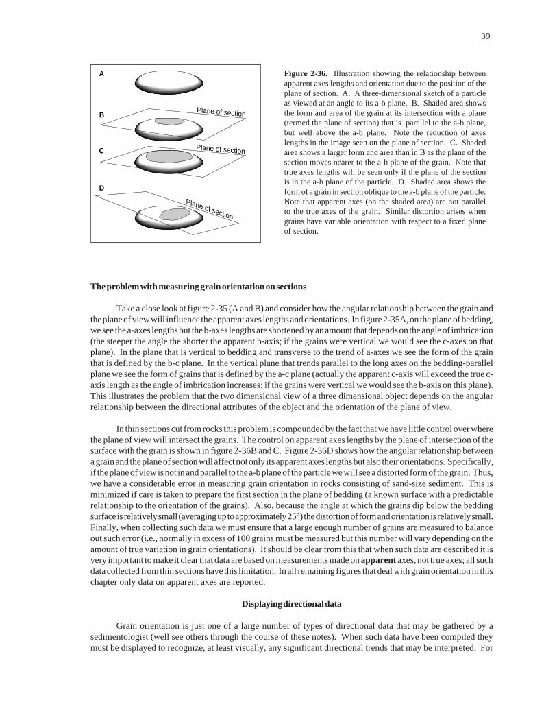
39

The problem with measuring grain orientation on sections

Take a close look at figure 2-35 (A and B) and consider how the angular relationship between the grain andthe plane of view will influence the apparent axes lengths and orientations. In figure 2-35A, on the plane of bedding,we see the a-axes lengths but the b-axes lengths are shortened by an amount that depends on the angle of imbrication(the steeper the angle the shorter the apparent b-axis; if the grains were vertical we would see the c-axes on thatplane). In the plane that is vertical to bedding and transverse to the trend of a-axes we see the form of the grainthat is defined by the b-c plane. In the vertical plane that trends parallel to the long axes on the bedding-parallelplane we see the form of grains that is defined by the a-c plane (actually the apparent c-axis will exceed the true c-axis length as the angle of imbrication increases; if the grains were vertical we would see the b-axis on this plane).This illustrates the problem that the two dimensional view of a three dimensional object depends on the angularrelationship between the directional attributes of the object and the orientation of the plane of view.

In thin sections cut from rocks this problem is compounded by the fact that we have little control over wherethe plane of view will intersect the grains. The control on apparent axes lengths by the plane of intersection of thesurface with the grain is shown in figure 2-36B and C. Figure 2-36D shows how the angular relationship betweena grain and the plane of section will affect not only its apparent axes lengths but also their orientations. Specifically,if the plane of view is not in and parallel to the a-b plane of the particle we will see a distorted form of the grain. Thus,we have a considerable error in measuring grain orientation in rocks consisting of sand-size sediment. This isminimized if care is taken to prepare the first section in the plane of bedding (a known surface with a predictablerelationship to the orientation of the grains). Also, because the angle at which the grains dip below the beddingsurface is relatively small (averaging up to approximately 25°) the distortion of form and orientation is relatively small.Finally, when collecting such data we must ensure that a large enough number of grains are measured to balanceout such error (i.e., normally in excess of 100 grains must be measured but this number will vary depending on theamount of true variation in grain orientations). It should be clear from this that when such data are described it isvery important to make it clear that data are based on measurements made on apparent axes, not true axes; all suchdata collected from thin sections have this limitation. In all remaining figures that deal with grain orientation in thischapter only data on apparent axes are reported.

Displaying directional data

Grain orientation is just one of a large number of types of directional data that may be gathered by asedimentologist (well see others through the course of these notes). When such data have been compiled theymust be displayed to recognize, at least visually, any significant directional trends that may be interpreted. For

Plane of section

A

D

Plane of sectionC

Plane of sectionB

Figure 2-36. Illustration showing the relationship betweenapparent axes lengths and orientation due to the position of theplane of section. A. A three-dimensional sketch of a particleas viewed at an angle to its a-b plane. B. Shaded area showsthe form and area of the grain at its intersection with a plane(termed the plane of section) that is parallel to the a-b plane,but well above the a-b plane. Note the reduction of axeslengths in the image seen on the plane of section. C. Shadedarea shows a larger form and area than in B as the plane of thesection moves nearer to the a-b plane of the grain. Note thattrue axes lengths will be seen only if the plane of the sectionis in the a-b plane of the particle. D. Shaded area shows theform of a grain in section oblique to the a-b plane of the particle.Note that apparent axes (on the shaded area) are not parallelto the true axes of the grain. Similar distortion arises whengrains have variable orientation with respect to a fixed planeof section.

40

example, if we have a set of measurements of the imbrication direction of a number of particles we will need todetermine whether the data are consistent and what is the mean imbrication direction. The imbrication directionwill indicate the upstream direction with respect to the current that deposited the sediment. If such deposits containfine gold particles we might want to know where the sediment came from so that we might find its source; theimbrication direction will point towards that source. Statistical treatment of directional data will be considered inthe next section.

Sedimentologists display directional data on a form of circular histogram that is commonly referred to as arose diagram. Consider the directional data plotted in the form of an ordinary histogram in figure 2-37A. The numberof measurements (i.e., the frequency) in 30° classes is shown over the range 0 to 360° (a full circle; north is generallytaken to be towards 0°). You can see from this histogram that the modal direction is in the range 120-149° (thesoutheast) and the data varies almost symmetrically about that mode. Inset in figure 2-37A is a rose diagram forthe same data and it shows the same trend. However, it is obviously easier to visualize the directional significanceof the data plotted on the rose diagram. Figure 2-37B shows another set of data plotted on a regular histogram anda rose diagram. In this case we can recognize two prominent modes, one from 0 to 29° and another from 330 to 359°.It is not readily apparent how these two modes are related until we look at the form of the rose diagram (inset in Fig.2-37B). The rose diagram more clearly shows the overall trend of the directional data (in this case pointing towardsthe north-northwest). The visual impact of a rose diagram is important when we compare different data sets andparticularly when we plot such diagrams on maps.

Figure 2-38 illustrates how rose diagrams are constructed using the example of data describing imbricationdirection. The class intervals define the angle of curvature of pie-shaped segments that have a length equal to thenumber (this may be expressed as a percentage) of observations per class (i.e., the frequency per class). In figure2-38 the class interval is 30° and the scale of frequency is shown radiating from the centre of the circle. The centreof a rose diagram is commonly reserved to note the total number of observations used to construct it.

Two forms of rose diagram are shown in figure 2-38 based on the data given in the table. In rose A the distance(L) from the centre of the circle to each value representing the number of observations per class (N) is equal to the

Fre

qu

ency

(Num

ber

of o

bser

vatio

ns p

er c

lass

)

0˚N

90˚E

180˚S

270˚W

360˚N

0

5

10

15

0˚N

90˚E

180˚S

270˚W

360˚N

0

5

10

15

Direction Direction

0 5 10 15

Number of observations

62

N N

0 5 10 15

Number of observations

62

Figure 2-37. Examples of directional data plotted as conventional histograms and as rose diagrams (inset).

41

value itself; that is L = N in whatever units you like; the distance between each value on the frequency scale is equal.Thus, a segment of the rose corresponding to a class containing 5 observations is five times longer (extendingoutward from the origin) than a segment corresponding to a class containing only 1 observation. Rose B showsanother frequency scale that many argue is more appropriate. In the case of Rose B the distance from the centreof the circle to any value is given by L = N0.5. Therefore, the spacing of the frequency increments decreases outwardform the centre of the circle. The reason for this is that in this type of diagram the frequency of observations perclass is not shown in terms of the length of the segments but is shown by the relative area of each segment. Forexample, when such a scale is used the area of a segment of the rose representing 5 observations is equal to fivetimes the area of a segment representing 1 observation. Because rose diagrams are used for their visual impact,some sedimentologists argue that this is a more representative scale than the linear scale. Note the difference inthe form of the two roses in figure 2-38. The equal area scale reduces the visual impact of the difference betweenintervals (compare the relative sizes of the segments corresponding to the 180-209° and 210-239° intervals). All rosediagrams in these notes will be presented with a linear frequency scale.

The form of the rose diagram indicates the directional trends of the data in a visually useful manner. Likeany such data, the distribution may have one or more modes and is termed unimodal if one mode is present, bimodalif two modes are present (bipolar if the modes are at 180° to each other) or polymodal if more than two modes arepresent (Fig. 2-39). Also, the data may vary symmetrically or asymmetrically about the mode(s). The interpretationof the form of a rose will depend on what directional attributes of a sediment have been measured to collect the data.In the case of grain imbrication, the rose points towards the average direction of dip of the a-b planes of the particlesand this direction is at 180° to the current that formed the imbrication. Therefore, the rose shown in figure 2-38 showsa mean imbrication direction to the south-southeast, produced by a current flowing towards the north-northwest.Many other directional attributes point in the direction of the current under which they formed and the roses thatthey produce will point directly in the flow direction.

Many types of directional data are like that shown in figure 2-38 based on grain imbrication; i.e., theimbrication direction is a specific direction determined by the dip of the a-b plane of a particle. However, manyfeatures for which directional data may be collected do not point to a specific direction. Consider the long axisorientation of a particle; it does not point in a given direction but rather lies on a directional trend. For example,an a-axis oriented towards 10° has the same orientation as an a-axis oriented towards 190°. Thus, the a-axis of thegrain is said to trend along 10-190°. Such directional data are said to be bidirectional; pointing in either of twodirections which are at 180° to each other. Figure 2-40 shows how such data are commonly dealt with in theconstruction of rose diagrams. Note that rose diagrams based on bidirectional data are symmetrical with only oneside of the rose representing actual measurements and the other side is just its mirror image to give the impressionof the bidirectional nature of the data. Figure 2-41 shows the forms of rose diagrams produced by measuring grain

0˚

90˚

180˚

270˚

30˚

60˚

120˚

150˚210˚

240˚

300˚

330˚

12

3

45

12

34

50˚

30˚

60˚

90˚

120˚

150˚180˚

210˚

240˚

270˚

300˚

330˚Raw data: 96, 121, 135, 146, 152, 160, 165, 172, 178, 185, 186, 201, 209, 212, 219

Class Interval Frequency

90-119˚ 1120-149˚ 3150-179˚ 5180-209˚ 4210-239˚ 2 Total: 15

A B

15 15

Equal length Equal area

(degrees)

frequency frequencyData recording imbrication direction

Figure 2-38. Illustration showing the construction of a rose diagram. See text for explanation.

42

Figure 2-39. Classification of form of rose diagram. After Pettijohn, Potter and Siever, 1973. See text for explanation.

28

Bimodal

22

Unimodal

N N

44

Polymodal

N

29

Bipolar

Figure 2-40. Illustration showing the significance of a rose diagram basedon bidirectional data. In this case, the rose diagrams represent the long axisorientation of grains seen on a bedding plane; one particle is shown but theroses represent a population of grains with a mean a-axis orientationparallel to that shown on the example particle. Because the a-axis of aparticle (like that shown in the illustration) has a trend but no absolutedirection, either of the top roses may equally well describe its orientation.However, visually these two roses give two diametrically opposing impres-sions of the a-axes they represent because they impart a sense of directionto the data; the left-hand rose suggests that the axes point to the west andthe right-hand rose suggests that the axes point to the east. To counter thisperceived sense of direction it is common practice to construct rosediagrams that are symmetrical, as shown in the lower part of the figure.Note that the lower rose has doubled in size without increasing the numberof measurements on which it is based.

N68 68

68

axis of symmetry

+

=

axes orientation in sediment with the anisotropic fabrics described in the previous section. A word of caution: becareful to note what is represented by any rose diagram. For example, truly directional data, based on structuresproduced by tidal currents that flow in directions that vary by 180° over time, may produce essentially symmetricalroses like those shown in figures 2-40 and 2-41.

Statistical treatment of directional data

Normally, directional data are collected in sets of N observations from some particular deposit or associatedstructure. Like grain size data, a set of directional data will be distributed about some mean direction and will havea range of variation about the mean direction. Unlike grain size data, directional data cannot be treated by regularstatistics because each value in a set is a vector quantity and each vector has two components: each observationin a set of directional data will have a direction (θ) and a magnitude (normally each vector has unit magnitude, i.e,its magnitude equals 1; such a vector is termed a unit vector). The descriptive statistics are similar to those appliedto scalar quantities (like grain size) but their computation is fundamentally different. Without going into the detailsof vector algebra this section provides an outline of the various statistics and their implications.

For any distribution of directional data the mean is the resultant vector (sometimes called the vector mean)formed by summing all of the unit vectors that comprise the data set (e.g., Fig. 2-42). Once again, the resultant vector

includes a direction (θ ) and a magnitude (R):

θ = −tan 1 w

vEq. 2-31

43

Note that θ must be corrected as follows: if w > 0 and v > 0 then θ = Eq. 2-31;

if w > 0 and v < 0 or w < 0 and v < 0 then θ = Eq. 2-31 + 180˚;

if w < 0 and v > 0 then θ = Eq. 2-31 + 360˚

and

R v w= +2 2 Eq. 2-32

where

w ni ii

N or NC

==∑ sinθ

1

Eq. 2-33

and

v ni ii

N or NC

==∑ cosθ

1

Eq. 2-34

and N is the number of observations in the data set. Note that directional data may be treated as either individualmeasurements (i.e., as raw data) or grouped data (i.e., data are expressed as frequency per class interval). In thecase of ungrouped data n

i is equal to 1 (unit magnitude of each vector) and θ

i represents each of the measured

directions (from i = 1 to N) of the N vectors in the data set. When data are grouped the quantities above are: ni is

the number of observations in each class interval (from i = 1 to NC) and θi is the mid-points of each class interval

(from i = 1 to NC) and NC is the number of class intervals (i.e., NC = 360°/CI, where CI is the class interval in degrees).

The magnitude of the resultant vector can also be expressed as a percentage (L) of the total number of

Figure 2-42. Example of the derivation of a resultant vector(syn. vector mean; large arrow) by the summation of unit vectors(small numbered arrows). Each unit vector has the directionshown and a magnitude (r

i) of 1. Use Equations 2-31 to 2-35 to

demonstrate the calculation of the direction and magnitude ofthe resultant vector. Note that the arithmetic mean would be146° and clearly not representative of the three vectors.

Figure 2-41. Rose diagrams representing two forms of anisotropic fabric (see Fig. 2-35 but note that the blocks shown hereare rotated at 180° to the blocks in Fig. 2-35).

A

BC

North

68

bedding

S N

68

bedding

W E

C

B

a(t)b(i)

N

A68

N

A

BC

North

68

bedding

S N

68

bedding

W E

A

C

B

a(p)a(i)68

(i) (ii)

1

+

2

3+

=

θ1

= 346˚

r1

= 1

θ2

= 24˚

r2

= 1

θ3

= 67˚

r3

= 1

θ = 25.5˚

R = 2.52

L = 84%

44

observations (or more specifically, as a percentage of the total length of the unit vectors that comprise the dataset):

LR

N= ×100 Eq. 2-35

The magnitude of the resultant vector, particularly when it is expressed as a L reflects the amount ofdispersion of the data (i.e., the degree of variation of directions in the data set). Another, more important, measureof the dispersion of the distribution of directional data is p (defined as the probability that the data are from apopulation that is uniformly distributed) where:

p e L N= − ×1 0 00012( . ) Eq. 2-36

p ranges in value from 0 to 1 where p = 0 indicates that there is no chance that the data are uniformly distributed(i.e., the data are from a population that has a preferred orientation) and p = 1 indicates that the data are from apopulation that is definitely uniformly distributed (i.e., the population has no preferred orientation).

Table 2-4 provides an example of the treatment of directional data, both as ungrouped and grouped data.With a little experience it is possible to acquire some intuition about these statistical properties on the basis of theform of the rose diagram representing a data set.

Interpretation of grain orientation

In the previous section one interpretive use of imbrication direction has already been established; it pointsin the direction 180° to the direction of the current that acted on the particles. Most workers who have includedgrain fabric in studies of ancient rocks have used their results to reconstruct paleoflow directions. However, thereare several other ways in which fabric may be interpreted. To begin with, the anisotropic fabrics can be interpretedin terms of how the particles moved under a flowing current. The a(t)b(i) fabric is produced by currents that rollthe particles along the bottom. This is the typical fabric of gravel size sediment; because of their large mass it isdifficult to move them in any other way but to roll them along the bottom. In contrast, the a(p)a(i) fabric tends tobe the most common fabric in sands and is thought to develop under relatively high rates of deposition and sedimenttransport and high sediment concentration. Thus, for a given grain size a(p)a(i) fabrics in gravel will be producedunder much more energetic currents than those that produce a(t)b(i) fabric. The classic experimental studies ofgravel orientation by Johansson (1965, 1976) are required reading for anyone concerned with gravel fabrics.Isotropic fabrics may result from rapid deposition of thick slurries which restrict the independent movement of aparticle, hindering the establishment of a preferred orientation.

Figure 2-43 shows an example of a complex anisotropic fabric based on data collected from a sandstone thatwas deposited in a shallow-marine environment. Two major modes, at 90° to each other, are clearly seen on the rosediagram. This fabric was produced by oscillating currents induced by storm waves in a shallow sea and thebimodality is interpreted in terms of a mixture of transport modes at the time of deposition. The NW-SE moderepresents grains with long axes aligned normal to the wave-induced current; these grains were rolled along thebed. The SW-NE mode represents grains that were aligned with their a-axes trending parallel to the current andrepresent sand that was rapidly deposited from suspension. In this particular case, the bimodality of the fabricreflects processes that act under currents produced by waves and may provide a basis for inferring wave-inducedcurrents in other ancient deposits.

In most sands the imbrication angles of grains range from 5 to 20°, although higher angles have been recordedin sands that are very rapidly deposited by sediment gravity flows. Some research has suggested that imbricationangle may also reflect the power of the current that act to align particles. Experiments by Gupta et al. (1987) showeda distinct steepening of imbrication angles with increasingly strong flows. However, recent experiments have shedsome doubt on the relationship between imbrication angle and flow strength (Arnott and Hand, 1989).

Results of one recent study have suggested that grain imbrication may be particularly useful in interpretingthe nature of transporting currents. Specifically, the results suggested that variation in imbrication angle through

45

Table 2-4. Example of the statistical treatment of ungrouped and grouped directional data.

Raw data: 184 187 191 196 198 201 204 205(degrees) 205 207 208 210 212 214 216 222

224

Grouped data:Class Interval Midpoint Frequency

180-189° 184.5° 2190-199° 194.5° 3200-209° 204.5° 6210-219° 214.5° 4220-229° 224.5° 2

Total: 17

Treatment of ungrouped data:

w ni ii

N= ∑ = −

=sin .θ

17 04 v ni i

i

N= ∑ = −

=cos .θ

115 13

θ θ θ=−

−= < < = − + ∴ = + =−tan

.

.. ; . .1 7 04

15 1324 95 180 24 95 180 204 95 w 0 and v 0 then Eq.2 31 o o

R L= − + − = = ×( . ) ( . ) . ;.

15 13 7 04 16 6916 69

172 2 100 = 98.17%

p e= = ×− × × −1 98 17 17 0 0001 82

7 67 10( . . ) .

Treatment of grouped data:

w ni ii

NC= ∑ = + + + + = −

=sin sin . sin . sin . sin . sin . .θ

12 184 5 3 194 5 6 204 5 4 214 5 2 224 5 7 06

o o o o o

v ni ii

NC= ∑ = + + + + = −

=cos cos cos cos cos cos. . . . . .θ

12 184 5 3 194 5 6 204 5 4 214 5 2 224 5 15 08

o o o o o

θ θ θ=−

−= < < = − + ∴ = + =−tan

.

.. ; . .1 7 06

15 0825 09 180 25 09 180 205 09 w 0 and v 0 then Eq.2 31 o o

R L= − + − = = ×( . ) ( . ) . ;.

15 08 7 06 16 6516 65

172 2 100 = 97.95%

p e= = ×− × × −1 97 95 17 0 0001 82

8 25 10( . . ) .

Note the slight discrepancy between calculations based on grouped and ungrouped data due to the useof the class mid-points in the case of grouped data.

46

151

N

10 observations

Apparent a-axes orientations froma shallow marine sandstone

FLOW

Figure 2-43. An example of a complex anisotropic fabric. Rose diagramshows the trend of apparent long axes seen in the plane parallel to beddingfrom the Upper Cretaceous Chungo Member (Wapiabi Formation) in theRocky Mountain Foothills. Note the prominent bimodality of the rose. Seetext for explanation. After Cheel and Leckie (1992).

a sediment may record changes in current strength and direction over time. Figure 2-44 shows data collected bydetermining the mean imbrication angle in thin (0.1 to 0.2 mm) vertically contiguous layers through a sediment. Inthe plots in figure 2-44 each point represents the mean imbrication angle (and direction ) in one such layer. Therose diagrams in figure 2-44 are based on all data in the subjacent plot. Figure 2-44 A shows data from the depositsof a river in which currents flowed consistently in the same direction over the course of deposition of the sediment(such currents are said to be “unidirectional”). Within these river deposits the mean imbrication angle is atapproximately 13°, dipping into the current. There is little systematic variation in imbrication angle through thedeposit, reflecting the constant nature of the flow strength over the period of deposition. For comparison, figure2-44B shows data from the deposits of a shallow marine setting that was influenced by waves, specifically powerfulstorm-generated waves. The currents produced by such waves would flow back and forth over 180° over periodson the order of 10 seconds, and are termed oscillatory or “bidirectional” currents. In contrast to the river-formedfabric, the mean imbrication angle is parallel to bedding, reflecting the alternating direction of the current (i.e., thenumber of grains that are imbricate in one direction are essentially cancelled out by the equal number of grains thatare imbricate in the opposing direction). The plot showing variation in imbrication through the shallow marinesandstone is also strikingly different: there is wide variation in imbrication angle and it appears to vary symmetricallyabout a mean of 0°. Not only is this variation symmetrical, but it is also has a cyclicity that can be proven statistically.The cyclic variation in imbrication angle through the deposit records variation in the magnitude of flow strengthunder waves: flow strength decreases, from a maximum in one direction, to zero and then increases to a maximumin the opposing direction. Thus, detailed studies of the variation in imbrication angle in sediment may provide apowerful tool in distinguishing the products of unidirectional and oscillatory currents.

DIS

TA

NC

E A

BO

VE

DA

TU

M (

MM

)

0

2

1

-90 900

θ341

FLOW

ANGLE (˚)

B. Fabric produced by oscillatorycurrent under waves in an

ancient shallow sea

ANGLE (˚)

-90 0 900

1

2

3

4

θ

186

FLOW

A. Fabric produced by unidirectionalcurrent in an ancient river

B BFigure 2-44. Comparison of the fabric of sandstonesdeposited in fluvial (A) and shallow-marine (B)settings. See text for discussion. After Cheel(1991).