(Why) Does Order Flow Forecast Exchange Rates?∗

Pasquale DELLA CORTE Dagfinn RIME

Imperial College London Norges Bank & NTNU

p.dellacorte@imperial.ac.uk dagfinn.rime@norges-bank.no

Lucio SARNO Ilias TSIAKAS

Cass Business School & CEPR University of Guelph

lucio.sarno@city.ac.uk itsiakas@uoguelph.ca

Preliminary

October 12, 2011

∗Acknowledgements: We thank UBS for providing the customer order flow data used in this paper. Sarnoacknowledges financial support from the Economic and Social Research Council (No. RES-062-23-2340). Tsiakasacknowledges financial support from the Social Science and Humanities Research Council of Canada. Correspondingauthor: Lucio Sarno, Cass Business School, City University, 106 Bunhill Row, London EC1Y 8TZ, UK.

(Why) Does Order Flow Forecast Exchange Rates?

Abstract

We investigate the predictive information content of order flow for exchange rate returns, usinga unique data set on daily end-user transactions for nine exchange rates across four customer typesfrom 2001 to 2011. We find that a multi-currency trading strategy based solely on customer order flowstrongly outperforms the popular carry trade strategy. More importantly, the excess portfolio returnsgenerated from conditioning on customer order flow can be largely replicated using a combination ofstrategies based on publicly available information. This is consistent with the notion that order flowaggregates disperse public information about economic fundamentals that are relevant to exchangerates.

Keywords: Order Flow; Foreign Exchange; Market Microstructure; Forecasting; Asset Allocation.

JEL Classification: F31; G11.

1 Introduction

The foreign exchange (FX) is a decentralized market comprising two distinct groups of participants:

dealers and end-user customers. Dealers act as financial intermediaries who facilitate trades by

quoting prices at which they are willing to trade with customers. The trades between dealers and

customers are not transparent, however, since prices and transaction volumes are only observed by

the two transacting counterparties. Therefore, customer orders are an important source of private

information to dealers as, for example, they may signal the customers’interpretation of public news

and future risk premia. This private information is then revealed to the rest of the market when

dealers trade with each other motivated primarily by liquidity and inventory concerns.1 Trades

between dealers account for 38.9% of FX turnover and the remainder is customer trades (Bank of

International Settlements, 2010).2

This trading mechanism implies that customer order flow may be a predictor of future FX excess

returns. Order flow is a measure of the net demand for a particular currency defined as the value of

buyer-initiated orders minus the value of seller-initiated orders.3 The argument is as follows (see, e.g.,

Evans and Lyons, 2005, 2006, 2007). The spot exchange rate is the rate quoted by FX dealers and

hence reflects the dealers’information set. If dealers first receive the private information conveyed by

customer order flow and subsequently incorporate it in their quotes, then customer order flow should

be able to forecast FX excess returns. Note that the information conveyed by customer order flow

can only be used by the dealer who facilitated the transaction as it is not observed by other market

participants. Furthermore, customers are heterogeneous in their motivation for trading, attitude

towards risk and horizon leading them to adopt different trading strategies. Therefore, different

customer groups will provide dealers with different information. Through interdealer trading this

information will be aggregated and mapped to a price thus establishing a transmission mechanism

from customer order flow to the exchange rate.

To put it in perspective, order flow is the centerpiece of the market microstructure approach to

1 In the interdealer market, dealers have access to two different trading channels: they can trade directly with eachother or through brokers, where the latter includes FX trading platforms such as Reuters and Electronic BrokingSystems. The direct interdealer trades are private since the bid and ask quotes, the amount and direction of tradeare not announced to the rest of the market. The second channel is more transparent as electronic brokers announcebest bid and ask prices and the direction of all trades. However, this information is only available to dealers (see, e.g.,Bjonnes and Rime, 2005).

2For further details on the institutional structure of the FX market, see, for example, Lyons (2001), Bjonnes andRime (2005), Evans and Lyons (2006), Sager and Taylor (2006), and Evans (2011).

3Earlier studies use a simpler definition of order flow as the number (not value) of buyer-initiated trades minus thenumber of seller-initiated trades (e.g., Evans and Lyons, 2002).

1

exchange rates pioneered by Evans and Lyons (2002). This line of research has emerged as an exciting

alternative to traditional economic models of exchange rate determination, which despite thirty years

of research have had limited success in explaining and predicting currency movements. As a result,

exchange rates are thought to be largely disconnected from macroeconomic fundamentals in what is

widely known as the “exchange rate disconnect” puzzle (Obstfeld and Rogoff, 2001). The market

microstructure literature asserts that transactions can affect prices because they convey information.

News can be impounded directly in currency prices or indirectly via order flow (Evans and Lyons,

2008).4 Order flow can also affect the price for reasons unrelated to publicly available news (e.g.,

changing risk aversion, liquidity and hedging demands).

This paper investigates the predictive ability of customer order flow using a new and comprehen-

sive order flow data set obtained from UBS, a global leader in FX trading. The data set disaggregates

customer order flows into trades executed between UBS (the dealer) and four segments (customers):

asset managers, hedge funds, corporates and private clients. The disaggregated nature of the data

is crucial as it allows us to determine whether conditioning on the four different types of UBS cus-

tomers, as opposed to using the aggregated order flow typically used in the literature, can improve

the explanatory and predictive power of order flow for exchange rate returns. Overall, this is a

rich data set that contains the US dollar value of daily order flows over an 11-year sample period

ranging from January 2001 to May 2011 and covers nine major currencies relative to the US dollar.

Therefore, it provides us with a unique opportunity to examine the predictive ability of customer

order flow over a long sample and a large set of exchange rates.

Armed with these data, our paper has two main objectives. First, we assess the predictive

ability of the four types of customer order flow on FX excess returns from the point of view of an

investor (or dealer) implementing a multi-currency dynamic asset allocation strategy. We choose a

trading strategy to assess the predictive ability of customer order flow since it is through trades that

customers reveal their information. Second, we relate the excess portfolio returns generated from

order flow strategies to the excess portfolio returns of other public information strategies commonly

used in the literature. In other words, if customer order flow has predictive private information that

4Evans and Lyons (2008) provide an excellent example of the indirect channel to the price adjustment process.Consider a scheduled macro announcement on US GDP growth that is higher than the expectation of market partici-pants. Suppose that everyone agrees that the GDP announcement represents good news for the US dollar but there arediverse opinions as to how large the appreciation should be relative to the Japanese yen. In this case, some participantsmay view the initial rise in the yen/dollar spot rate as too large while others as too small. Those who view the riseas too small will place orders to purchase the dollar, while those who view the rise as too large will place orders tosell. Positive order flow signals that the initial yen/dollar spot rate was below the balance of opinion among marketparticipants and vice versa.

2

can consistently generate excess portfolio returns, can we replicate these returns by conditioning

on publicly available (e.g., macroeconomic) information? For example, to what extent do customer

orders reflect changes in interest rates, real exchange rates or monetary fundamentals? Finally,

is there a component of the predictive information of customer order flows (e.g., an alpha in the

trading strategies) that is completely private and hence cannot be replicated by combining public

information?

In answering these questions, we adopt the carry trade as the benchmark for assessing the per-

formance of order flow strategies. This is a popular trading strategy that borrows in low-interest

rate currencies and lends in high-interest rate currencies, and has been the focus of recent academic

research (e.g., Burnside, Eichenbaum, Kleshchelski and Rebelo, 2011; Lustig, Roussanov and Verdel-

han, 2011; Menkhoff, Sarno, Schmeling and Schrimpf, 2011). Note that a plain version of the carry

trade is based on the assumption that the spot exchange rate follows a random walk, which is the

benchmark in the literature on exchange rate forecasting ever since the seminal paper of Meese and

Rogoff (1983).

We find that the order flow strategies conditioning separately on each individual customer type

strongly outperform the standard carry trade strategy as they deliver a superior Sharpe ratio net of

transaction costs. This is especially true in the post-2007 sample. The strategy that conditions on all

four customer flows together tends to perform the best in sample and out of sample. In particular, a

mean-variance investor is willing to pay an out-of-sample performance fee of up to 800 basis points

annually to switch from the carry trade to conditioning on customer order flow. Therefore, there is

high economic value in the predictive information of customer order flow, which is magnified when

using all segments of the disaggregated data.

Furthermore, 60% to 70% of the excess portfolio returns generated from conditioning on order

flow can be replicated using a combination of strategies based on publicly available information.

These strategies include the random walk, forward premium, purchasing power parity, monetary

fundamentals, Taylor rule, cyclical external imbalances and momentum. Hence publicly available

information captured by variables such as interest rates, past values of exchange rates, inflation,

money supply, output, external imbalances and momentum is key in determining the net demand

for currencies as observed in FX order flow. More importantly, however, once the role of public

information strategies is accounted for, there is no remaining alpha for the order flow strategies. We

conclude, therefore, that the information conveyed by customer order flow is a particular aggregation

of public information. Customers simply interpret and use public information, each in their own way.

3

Finally, the way customer order flow aggregates public information is not constant over time. We

find evidence of strong time variation in the relative importance of different strategies driving order

flow. For example, while the carry trade is a critical driver of order flow during the pre-crisis period,

after the crisis erupted in July 2007 and the carry trade collapsed, it is replaced by purchasing power

parity and monetary fundamentals. This is consistent with the scapegoat theory of Bacchetta and

van Wincoop (2004, 2006), which suggests that the relation between macroeconomic fundamentals

and the exchange rate is highly unstable. This parameter instability is due to the different weight

that on a given day traders assign to a given macroeconomic indicator as the market rationally

searches for an explanation for the observed exchange rate change. A variable can be given excessive

weight a one day and zero weight the next day. As a result, different observed variables become

scapegoats. Bacchetta and van Wincoop (2004, 2006) term this “rational confusion”about the true

source of exchange rate fluctuations. In the short run, rational confusion plays an important role in

disconnecting the exchange rate from observed fundamentals, but allows them to be connected in

the long run.

The remainder of the paper is organized as follows. In the next section we describe the data used

in the empirical analysis, with particular emphasis on the UBS data set for FX order flows. Section

3 reviews the literature on models that link order flow, exchange rates and the macroeconomy. The

set of empirical models based on public information are described in Section 4. In Section 5 we

present the mean-variance framework for measuring the economic value of conditioning on order flow

in the context of a dynamic asset allocation strategy. Section 6 discusses the results from estimating

the empirical models conditioning on order flow and comparing their performance to the carry trade

strategy. It also analyzes the relation between the excess returns generated by the information in

order flow and the excess returns obtained from public information models. Section 7 summarizes

the key results and concludes.

2 Data and Preliminaries

2.1 Data Sources

The empirical analysis uses customer order flows, spot and forward rates, interest rates and a set

of macroeconomic variables for nine exchange rates relative to the US dollar (USD): the Australian

dollar (AUD), Canadian dollar (CAD), Swiss franc (CHF), Euro (EUR), British pound (GBP),

Japanese yen (JPY), Norwegian kroner (NOK), New Zealand dollar (NZD) and Swedish kronor

4

(SEK). The data range from January 2001 to May 2011 and cover 2618 daily observations after

removing holidays and weekends.

The order flow data come from proprietary daily transactions between four end-user segments

(customer groups) and UBS. UBS is a global leader in the FX market with a market share in turnover

higher than 10%.5 Order flows are disaggregated into four segments: trades executed between UBS

and asset managers (AM), hedge funds (HF), corporates (CO) and private clients (PC). The asset

managers segment comprises long-term real money investors, such as mutual funds and pension

funds. Highly leveraged traders and short-term asset managers not included in the previous group

are classified as hedge funds. The corporates segment includes non-financial corporations that import

or export products and services around the world or have an international supply chain. Treasury

units of large non-financial corporations are treated as corporates unless they pursue an aggressive

(highly leveraged) investment strategy, in which case they are classified as hedge funds. The final

segment, private clients, includes wealthy clients with in excess of $3 million in investible liquid

assets. Private clients trade primarily for financial reasons and with their own money.

The order flow data are assembled as follows. Each transaction booked in the UBS execution

system at any of its world-wide offi ces is tagged with a client type. At the end of each business

day, global transactions are aggregated across the four segments. Order flow is measured as the

difference between the dollar value of purchase and sale orders for foreign currency initiated by UBS

clients. Specifically, let Vt be the dollar value of a transaction initiated by a customer at time t.

The transaction is recorded with a positive (negative) sign if UBS fills a purchase (sale) order of

foreign currency. Over time, order flow is measured as the cumulative flow of buyer-initiated and

seller-initiated orders. Each transaction is signed positively or negatively depending on whether

the initiator of the transaction (the non-quoting counterparty) is buying or selling. It follows that

positive order flow indicates a net demand of foreign currency whereas negative order flow a net

supply.6

The order flow data set used in our analysis is the most comprehensive in this literature to

date and is also unique in many respects. First, in contrast to most other empirical studies that

focus on interdealer data, we use customer order flow data disaggregated into the four segments

5Table C1 in the Appendix displays the top 10 global leaders in the FX market in terms of market share in annualturnover from 2001 to 2011 based on the Euromoney FX Survey.

6 It is important to note that order flow is distinct from transaction volume. Order flow is transaction volume that issigned. Microstructure theory defines the sign of a trade depending on whether the initiator (i.e., customer) is buyingor selling. Consider, for example, a sale of 10 units by a customer acting on a dealer’s quotes. Then transaction volumeis 10, but order flow is —10 (Lyons, 2001).

5

discussed above. Second, our data set spans more than 11 years of daily observations for nine

currency pairs and it comes from a major FX market leader. Although there are recent studies that

employ customer order flow data, they typically suffer from a number of limitations as they cover a

relatively short period of time, fewer currency pairs or a limited number of end-user segments. For

instance, Evans and Lyons (2005, 2006, 2007) and Evans (2010) employ six years of data for one

currency pair from Citibank. Cerrato, Sarantis and Saunders (2011) use six years of data for nine

currency pairs from UBS but, in contrast to this paper, their data are weekly; they have 317 weekly

observations compared to our 2618 daily observations. Froot and Ramadorai (2005) use seven years

of data for eighteen currency pairs from State Street, a global custodian bank. These are flow data

with primarily institutional investors, which are however aggregated, and hence cannot capture the

same diversity in currency demand as with the UBS end-user segments.

Third, most empirical studies use the number and not the dollar value of buyer-initiated and

seller-initiated transactions to measure order flow (e.g., Evans and Lyons, 2002). Finally, our order

flow data are raw data with minimal filtering. For instance, data are adjusted to take into account for

large merger and acquisition deals which are announced weeks or months in advance. Cross-border

merger and acquisitions involve large purchases of foreign currency by the acquiring company to

pay the cash component of the deal. These transactions are generally well-publisized and thus are

anticipated in advance by market participants. Furthermore, FX reserve managers, UBS proprietary

(prop) traders and small banks not participating in the interbank market are excluded from the

data set. Flows from FX reserve managers are stripped out due confidentiality issues, flows from

prop traders because they trade with UBS’s own money, while small banks often have non-financial

customers behind them.

The exchange rates are Thomson Reuters data obtained through Datastream. We use daily spot

and spot-next forward rates for the daily analysis, and end-of-month spot and one-month forward

rates for the monthly analysis. The exchange rate is defined as the US dollar price of a unit of

foreign currency so that an increase in the exchange rate implies a depreciation of the US dollar.

Most of the empirical work uses mid-quotes, but bid and ask quotes are used to construct transaction

costs as detailed in Section 5. For interest rates, we use daily (end-of-month) spot-next (one-month)

Eurodeposit rates from Datastream.

Turning to macroeconomic data, we obtain the narrow money index (M1) as a proxy for money

supply, the industrial production index (IPI) as a proxy for real output, and the consumer price index

(CPI) from the OECD statistics. These data are generally available at monthly frequency, with the

6

following exceptions that are published quarterly: IPI for Australia, New Zealand and Switzerland;

and CPI for Australia and New Zealand. For the inflation rate, we use an annual measure computed

as the 12-month log difference of CPI. For the output gap, we construct the deviations from the

Hodrick and Prescott (1997) filter as in Molodtsova and Papell (2009).7 We mimic as closely as

possible the information set available to central banks using quasi-real time data; although data

incorporate revisions, we update the Hodrick and Prescott (1997) trend each period so that ex-post

data is not used to construct the output gap. In other words, at time t we only use data up to t− 1

to construct the output gap.8 From OECD statistics, we also obtain annual data on the purchasing

power parity (PPP) spot exchange rate. Finally, we use the International Financial Statistics (IFS)

database to obtain quarterly data on external assets and liabilities, exports and imports of goods

and services, and GDP.9 Note that macroeconomic variables are only available at monthly or lower

frequency. We construct daily observations by fixing the latest available observations until a new

data point is again available.

We convert the data by taking logs, except for interest rates and order flows. Henceforth the

symbols st, ft, xt, it, mt, πt, yt and yt refer to the log spot exchange rate, log forward exchange

rate, order flow, interest rate, log money supply, inflation rate, log real output and log output gap,

respectively. We use an asterisk to denote the data (i∗t , m∗t , π

∗t , y

∗t and y

∗t ) for the foreign country.

The log of the PPP spot rate defines the log price level differential pt − p∗t . As in Gourinchas and

Rey (2007), we construct a global measure of cyclical external imbalances, labelled nxat, as a linear

combination of detrended log exports, imports, foreign assets, and liabilities relative to GDP.10

7Orphanides (2001) stresses the importance of using real-time data to estimate Taylor rules for the United States.However, Orphanides and van Norden (2002) show that most of the difference between fully revised and real-time datacomes from using ex-post data to construct potential output and not from the data revisions themselves.

8The output gap for the first period is computed using real output data from January 1990 to January 2001. In theHP filter, we use a smoothing parameter equal to 14,400 as in Molodtsova and Papell (2009).

9Unadjusted data are seasonally adjusted using dummy-variable regressions. Note that in the out-of-sample analysis,we perform the adjustment in a recursive fashion to avoid any look-ahead bias.10Following Gourinchas and Rey (2007) closely, we filter out the trend component in (log) exports, imports, foreign

assets, and liabilities relative to GDP using the Hodrick-Prescott filter. We then combine these stationary componentswith weights reflecting the (trend) share of exports and imports in the trade balance, and the (trend) share of foreignassets and liabilities in the net foreign assets, respectively. These time-varying weights are replaced with their sampleaverages to minimize the impact of measurement error. Finally, note that the Hodrick-Prescott filter and the constantweights are based on the full-sample information for the in-sample analysis. In the out-of-sample analysis, however,we implement the Hodrick-Prescott filter and compute the weights only using information available at the time of theforecast in order to avoid any look-ahead bias.

7

2.2 Preliminary Analysis

Table 1 reports UBS’s market share by customer type and its rank relative to the top 10 global FX

dealers from 2001 to 2011 based on the Euromoney annual survey. The table reveals that UBS has

been one of the top dealers for both the overall market and particular end-user segments. Although

the Euromoney survey uses different groupings than UBS, three of the groups defined by Euromoney

(real money, leveraged funds and non-financial corporations) seem to align well with three of the

UBS segments (asset managers, hedge funds and corporates).11 The table indicates that UBS is

among the top two banks trading against asset managers, among the top five banks for hedge funds,

and among the top ten banks with non-financial corporations.

Table 2 presents descriptive statistics for daily log exchange rate returns and order flows across the

four customer groups for the nine currency pairs from January 2001 to May 2011. Order flow tends

to be more volatile for asset managers and hedge funds and least volatile for the corporates. This

fits with the view that asset managers and hedge funds are very active traders, whereas corporate

clients trade mostly for import and export reasons.

Table 3 presents the contemporaneous cross-correlations between flows and returns: while asset

managers and hedge funds are positively correlated with exchange rate returns, corporate and pri-

vate clients are typically negatively correlated. These results are consistent with previous empirical

evidence reported by Evans and Lyons (2002) and Sager and Taylor (2006) indicating that asset

managers and hedge funds are informed traders (push customers) whereas corporate and private

clients act as overnight liquidity providers (pull customers).

3 Predictive Regressions

This section describes two sets of predictive regressions for exchange rate returns. The first set

conditions on the private information of customer order flows, whereas the second set conditions on

the public information contained in a battery of macroeconomic variables. All predictive regressions

have the following linear structure:

∆st+1 = α+ βxt + εt+1, (1)

11Euromoney also have a group called Banks, which covers so-called non-market making banks, often small banks,that do not find it worthwhile to have a presence in the interbank market but rather trade with other banks as theircustomer. There is no similar group in the UBS definitions, but these “customer-banks” often have non-financialcustomers behind them.

8

where st+1 is the nominal US dollar spot exchange rate for a particular currency at time t + 1,

∆st+1 = st+1 − st is the log-exchange rate return at time t + 1, xt is a predictive variable, α and

β are constant parameters to be estimated, and εt+1 is a normal error term. The empirical models

differ in the way they specify the predictive variable xt that is used to forecast exchange rate returns.

3.1 Order Flow Models

We capture the predictive information content in the orders of four heterogeneous customer groups

by estimating three types of predictive regressions for each exchange rate. The first type conditions

separately on the order flow of each of the four customers: asset managers (xAMt ), hedge funds

(xHFt ), corporates (xCOt ), and private clients (xPCt ). We call these the individual order flows. The

second type conditions on all four customer order flows, which we call the disaggregated order flows:

xt ={xAMt , xHFt , xCOt , xPCt

}. Finally, we condition on the sum of the four order flows, which we call

the aggregate (or total) order flow: xt = xAMt + xHFt + xCOt + xPCt . These regressions will determine

whether there is predictive information in customer order flows and the extent to which different

customer groups provide different information.

3.2 Public Information Models

3.2.1 Random Walk

The first specification based on public information is the driftless (or naive) random walk (RW)

model that sets α = β = 0. Since the seminal contribution of Meese and Rogoff (1983), this model

has become the benchmark in assessing exchange rate predictability. The RW model captures the

prevailing view in international finance research that exchange rates are unpredictable and forms

the basis of the widely used carry trade strategy in active currency management (e.g., Burnside,

Eichenbaum, Kleshchelski and Rebelo, 2011; Lustig, Roussanov and Verdelhan, 2011; Menkhoff,

Sarno, Schmeling and Schrimpf, 2011). The RW model is the benchmark to which we compare the

predictive regressions conditioning on order flow.

3.2.2 Forward Premium

The second specification uses the forward premium (FP) as a predictor:

xt = ft − st, (2)

where ft is the one-period log-forward exchange rate. The predictive regression using FP as con-

ditioning information captures deviations from the uncovered interest rate parity (UIP) condition.

9

Under risk neutrality and rational expectations, UIP implies that α = 0, β = 1, and the error term

is serially uncorrelated. However, empirical studies consistently reject the UIP condition and it is

a stylized fact that estimates of β often display a negative sign (e.g., Evans, 2011, Ch. 11). This

implies that high-interest rate currencies tend to appreciate rather than depreciate over time.12

3.2.3 Purchasing Power Parity

The third regression is based on the purchasing power parity (PPP) condition and sets

xt = pt − p∗t − st, (3)

where pt (p∗t ) is the log of the domestic (foreign) price level. This is equivalent to a trading strategy

that buys undervalued currencies and sells overvalued currencies relative to PPP. The PPP hypothesis

states that national price levels should be equal when expressed in a common currency and is typically

thought of as a long-run condition rather than holding at each point in time (e.g., Rogoff, 1996; and

Taylor and Taylor, 2004).

3.2.4 Monetary Fundamentals

The fourth regression conditions on monetary fundamentals (MF):

xt = (mt −m∗t )− (yt − y∗t )− st, (4)

where mt (m∗t ) is the log of the domestic (foreign) money supply and yt (y∗t ) is the log of the domestic

(foreign) real output. The relation between exchange rates and fundamentals defined in Equation (4)

suggests that a deviation of the nominal exchange rate from its long-run equilibrium level determined

by current monetary fundamentals requires the exchange rate to move in the future so as to converge

towards its long-run equilibrium. The empirical evidence on the relation between exchange rates

and fundamentals is mixed. On the one hand, short-run exchange rate variability appears to be

disconnected from the underlying monetary fundamentals in what is commonly referred to as the

“exchange rate disconnect”puzzle (Obstfeld and Rogoff, 2001). On the other hand, there is growing

evidence that exchange rates and monetary fundamentals are cointegrated, which requires that the

exchange rate and/or the fundamentals move in a way to restore and equilibrium relation between

them in the long run (e.g., Groen, 2000; Rapach and Wohar, 2002).12Note that we implicitly assume that covered interest parity (CIP) holds, so that the interest rate differential is

equal to the forward premium, ft − st = it − i∗t , where it and i∗t are the domestic and foreign nominal interest rates,respectively. In this case, testing UIP is equivalent to testing for forward unbiasedness in exchange rates (Bilson, 1981).There is ample empirical evidence that CIP holds in practice for the data frequency examined in this paper. For recentevidence, see Akram, Rime and Sarno (2008). The only exception in our sample is the period following Lehman’sbankruptcy, when the CIP violation persisted for a few months (e.g., Mancini-Griffoli and Ranaldo, 2011).

10

3.2.5 Taylor Rule

The fifth specification uses the Taylor (1993) rule defined as

xt = 1.5 (πt − π∗t ) + 0.1 (yt − y∗t ) + 0.1 (st + p∗t − pt) , (5)

where πt (π∗t ) is the domestic (foreign) inflation rate, and yt (y∗t ) is the domestic (foreign) output gap

measured as the percent deviation of real output from an estimate of its potential level computed

using the Hodrick and Prescott (1997) filter.13 The Taylor rule postulates that the central bank

raises the short-term nominal interest rate when output is above potential output and/or inflation

rises above its desired level. The parameters on the inflation difference (1.5), output gap difference

(0.1) and the real exchange rate (0.1) are fairly standard in the literature (e.g., Engel, Mark and

West, 2007; Mark, 2009; Molodtsova and Papell, 2009).

3.2.6 Cyclical External Imbalances

The sixth model employs as the predictive variable a bilateral measure of cyclical external imbalances

between the US and the foreign country. As in Gourinchas and Rey (2007), we construct nxat, a

global measure of cyclical external imbalances, which linearly combines detrended (log) exports,

imports, foreign assets, and liabilities relative to GDP. The bilateral measure of cyclical external

imbalances between the US and a foreign country is then constructed using a two-stage least squares

estimator as in Della Corte, Sarno and Sestieri (2011). We first regress the global nxat for the US

on a constant term and the global nxat for the foreign country, and then use the fitted value from

this contemporaneous regression as xt representing the proxy for the bilateral measure of cyclical

external imbalances between the US and the foreign country.

3.2.7 Momentum

The final specification uses the one—year rolling exchange rate return as the conditional mean of the

one-period ahead exchange rate. This strategy produces a long exposure to the currencies that are

trending higher, and a short exposure to the currencies that are trending lower.

13Note that in estimating the Hodrick-Prescott trend out of sample, at any given period t, we only use data up toperiod t− 1. We then update the trend every time a new observation is added to the sample. This captures as closelyas possible the information available at the time a forecast is made and avoids a look-ahead bias.

11

4 An Economic Assessment of the Predictive Ability of Order Flow

This section describes the framework for evaluating the ability of order flow to predict exchange rate

returns in the context of dynamic asset allocation strategies.

4.1 The Dynamic FX Strategy

We design an international asset allocation strategy that involves trading the US dollar vis-à-vis nine

major currencies: the Australian dollar, Canadian dollar, Swiss franc, Deutsche mark\euro, British

pound, Japanese yen, Norwegian kroner, New Zealand dollar and Swedish kronor. Consider a US

investor who builds a portfolio by allocating her wealth between ten bonds: one domestic (US), and

nine foreign bonds (Australia, Canada, Switzerland, Germany, UK, Japan, Norway, New Zealand

and Sweden). The yield of the bonds is proxied by eurodeposit rates. At each period t+1, the foreign

bonds yield a riskless return in local currency but a risky return rt+1 in US dollars. The expected US

dollar return of investing in a foreign bond is equal to rt+1|t = it+ ∆st+1|t, where rt+1|t = Et [rt+1] is

the conditional expectation of rt+1 and ∆st+1|t = Et [∆st+1] is the conditional expectation of ∆st+1.

Hence the only risk the US investor is exposed to is FX risk.

Every period the investor takes two steps. First, she uses the predictive regressions conditioning

on order flow or other public information to forecast the one-period ahead exchange rate returns.

Second, conditional on the forecasts of each model, she dynamically rebalances her portfolio by

computing the new optimal weights using the method discussed below. This setup is designed to

provide an economic assessment of the ability of order flow to predict exchange rates by informing us

whether conditioning on order flow leads to a better performing allocation strategy than conditioning

on the random walk or other standard public information models.

4.2 Mean-Variance Dynamic Asset Allocation with Transaction Costs

Mean-variance analysis is a natural framework for assessing the economic value of strategies that

exploit predictability in the mean and variance. Consider an investor who has a one-period horizon

and constructs a dynamically rebalanced portfolio. Computing the time-varying weights of this

portfolio requires one-step ahead forecasts of the conditional mean and the conditional variance-

covariance matrix. Let rt+1 denote the K × 1 vector of risky asset returns at time t + 1, Vt+1|t =

Et[(rt+1 − rt+1|t)(rt+1 − rt+1|t)′] the K ×K conditional variance-covariance matrix of rt+1, τ t+1 the

K × 1 vector of proportional transaction costs, and τ t+1|t = Et [τ t+1] the conditional expectation of

τ t+1.

12

Our analysis focuses on the maximum expected return strategy, which leads to an allocation on

the effi cient frontier. This strategy maximizes the expected portfolio return at each period t for a

given target portfolio volatility:

maxwt

rp,t+1|t = w′trt+1|t + (1− w′tι) rf − φt+1|t

s.t. σ∗p =(w′tVt+1|twt

)1/2,

(6)

where rp,t+1 is the portfolio return at time t+ 1, rp,t+1|t = Et[rp,t+1|t] is the conditional expectation

of rp,t+1, rf is the riskless rate, σ∗p is the target conditional volatility of the portfolio returns, and

φt+1|t is the conditional expectation of the total transaction cost for the portfolio in each period

defined as:

φt+1|t =

K∑i=1

τ i,t+1|t

∣∣∣wi,t − w−i,t∣∣∣ , (7)

where w−i,t = wi,t−1 (1 + ri,t) / (1 + rp,t).

The proportional transaction cost τ i,t+1|t for each asset i is computed as follows. We first define

the excess return of holding foreign currency for one period net of transaction costs as:

ernett+1 = sbt+1 − fat , (8)

where sbt+1 is the bid-quote for the spot rate at time t + 1, and fat is the ask-quote for the forward

rate at time t. This is the excess return for an investor who buys a forward contract at time t for

exchanging the domestic currency into the foreign currency at time t+ 1, and then, at time t+ 1 she

converts the proceeds of the forward contract into the domestic currency at the t+ 1 spot rate.

We can rewrite the above expression using mid-quotes to obtain:

ernett+1 =

(st+1 −

sat+1 − sbt+12

)−(ft +

fat − f bt2

)= (st+1 − ft)− ct+1, (9)

where st+1 and ft are the mid-quotes for the spot and forward exchange rate, and ct+1 = (sat+1−sbt+1+

fat − f bt )/2 represents the round-trip proportional transaction cost of the simple trading strategy. In

our setup, we define τ t+1 = ct+1/2 as the one-way proportional transaction cost for increasing or

decreasing the portfolio weight at time t+ 1 on a given foreign currency.

In the empirical implementation of the mean-variance strategy, we need to compute the time-

varying weights wt using information up to time t. These weights will determine the t+ 1 portfolio

return rp,t+1. However, the transaction cost τ t+1 relevant to t+1 returns will only be known ex post,

whereas the weights (which require an estimate of τ t+1) are set ex ante. We avoid this complication

13

by estimating τ t+1|t using the 3-month rolling average of the times series of τ t using information up

to time t. In short, to compute the weight wt we use the estimate τ t+1|t, but to compute the net

portfolio returns, which are known ex post, we use the realized τ t+1 value.

The inclusion of transaction costs in the optimization imply that the optimal solution for the

time-varying weights wt is not available in closed form but is obtained via numerical optimization.14

Once the optimal weights are computed, the return on the investor’s portfolio net of transaction

costs is equal to:

rp,t+1 = w′trt+1 +(1− w′tι

)rf − φt+1. (10)

Note that we assume that Vt+1|t = V , where V is the unconditional covariance matrix of exchange

rate returns. In other words, we do not model the dynamics of FX return volatility and correlation.

Therefore, the optimal weights will vary across the empirical exchange rate models only to the extent

that the predictive regressions produce better forecasts of the exchange rate returns.15

4.3 Performance Measures

We evaluate the performance of the exchange rate models using the Goetzmann, Ingersoll, Spiegel

and Welch (2007) manipulation-proof performance measure defined as:

M (rp) =1

(1− γ)ln

{1

T

T∑t=1

(1 + rp,t1 + rf

)1−γ}, (11)

where M (rp) is an estimate of the portfolio’s premium return after adjusting for risk, which can be

interpreted as the certainty equivalent of the excess portfolio returns. This is an attractive criterion

since it is robust to the distribution of portfolio returns and does not require the assumption of

a particular utility function to rank portfolios. The parameter γ denotes the investor’s degree of

relative risk aversion (RRA).

We compare the performance of the exchange rate model conditioning on order flow to the

benchmark RW by computing the difference :

P = M(r∗p)−M(rbp), (12)

14We use a linear transaction cost function because it can be solved globally and effi ciently as a convex portfoliooptimization problem. In practice, transaction costs may be a concave function of the amount traded. This happens,for example, when there is an additional fixed component to allow the total transaction cost to decrease as the amounttraded increases. This portfolio optimization problem cannot be solved directly via convex optimization (see Lobo,Fazel and Boyd, 2007).15See Della Corte, Sarno and Tsiakas (2009) for an empirical analysis of the effect of dynamic volatility on mean-

variance strategies in FX.

14

where r∗p are the portfolio returns of the order flow strategy and rbp of the benchmark RW.We interpret

P as the maximum performance fee an investor will pay to switch from the RW to the order flow

strategy. In other words, this performance criterion measures how much a mean-variance investor is

willing to pay for conditioning on better exchange rate forecasts. We report P in annualized basis

points (bps).

In the context of mean-variance analysis, perhaps the most commonly used performance measure

is the Sharpe ratio (SR). The realized SR is equal to the average excess return of a portfolio

divided by the standard deviation of the portfolio returns. We also compute the Sortino ratio (SO),

which measures the excess return to “bad”volatility. Unlike the SR, the SO differentiates between

volatility due to “up”and “down”movements in portfolio returns. It is equal to the average excess

return divided by the standard deviation of only the negative returns. In other words, the SO

does not take into account positive returns in computing volatility because these are desirable. We

compute both standard and robust measures of SR and SO, where the robust measures account for

the serial correlation in portfolio returns as in Lo (2002). Finally, we report the maximum drawdown

(MDD), which is the maximum cumulative loss from the strategy’s peak to the following trough. As

large drawdowns usually lead to fund redemptions, it follows that a reasonably lowMDD is critical

to the success of any fund.

4.4 Portfolios Based on Combined Forecasts

Our analysis has so far focused on evaluating the performance of individual empirical exchange

rate models relative to the random walk benchmark. Considering a large set of alternative models

that capture different aspects of exchange rate behaviour without knowing which model is “true”

(or best) inevitably generates model uncertainty. In this section, we explore ways to combine the

forecasts arising from the full set of competing predictive regressions. Although the potentially

superior performance of combined forecasts is known since the seminal work of Bates and Granger

(1969), applications in finance are only recently becoming increasingly popular (Timmermann, 2006;

Rapach, Strauss and Zhou, 2010).

Our empirical analysis estimates N predictive regressions for a vector of K exchange rates, which

provides an individual forecast ∆sj,t+1|t generated by each model j ≤ N for the vector of one-step

ahead exchange rate returns. We define the combined forecast ∆sc,t+1|t for the vector of exchange

15

rate returns as the weighted average of the N individual forecasts:

∆sc,t+1|t =N∑j=1

θj,t∆sjt+1|t, (13)

where {θj,t}Nj=1 are the ex ante combining weights determined at time t. The combining methods we

consider differ in how the weights are determined and can be organized into four types. The first type

uses simple averaging schemes: mean, median, and trimmed mean. The mean combination forecast

sets θj,t = 1/N in Equation (13); the median combination forecast is the median of{

∆sj,t+1|t}Nj=1;

and the trimmed mean combination forecast sets θj,t = 0 for the individual forecasts with the

smallest and largest values and θj,t = 1/ (N − 2) for the remaining individual forecasts in Equation

(13). These combined forecasts disregard the historical performance of the individual forecasts.

The second type of combined forecasts is based on Bates and Granger (1969) and Stock and

Watson (2004), and uses statistical information on the past performance of each individual model.

In particular, it sets the weights by computing the following mean squared error (MSE) forecast

combination:

θj,t =MSE−1j,t∑Nj=1MSE−1j,t

, MSEj,t =1

T

T∑t=1

(∆sj,t −∆sj,t|t−1

)2. (14)

The third type follows the Welch and Goyal (2008) “kitchen sink”(KS) model that incorporates

all N economic variables{xjt

}Nj=1

into a multiple predictive regression:

∆st+1 = α+N∑jβjx

jt + εt+1. (15)

The fourth and final type designs a “Fund of Funds”(FoF) strategy that equally invests in the

portfolio strategy based on the N models.

5 Empirical Results

5.1 The Correlation between Exchange Rates and Order Flow

We begin our empirical analysis by calculating the simple correlation between contemporaneous

currency order flows and FX returns at different horizons, as in Froot and Ramadorai (2005). Figure

1 displays for each customer type the average correlation across all exchange rates. The horizon is

reported in log-scale on the horizontal axis, running from the 1-day horizon (100 days) to 252 days

(> 102). To assess the significance of these correlations, the figure also shows the 90% confidence

intervals generated by 10, 000 replications under the null hypothesis that each order flow and FX

return series is independent and identically distributed (i.i.d.). Consistent with the contemporaneous

16

regression results discussed in the appendix, the correlations at the 1-day horizon are positive for

AM and HF flows, and negative for CO and PC flows. For AM flows, the correlations increase

markedly with horizon up to about 2.5 months, and are statistically significant up to a year. For

HF flows, the correlations are generally positive but less significant. For CO flows, the initial 1-day

correlations are negative and insignificant, but become positive for long horizons. The pattern for PC

is similar to CO. Overall, this preliminary analysis provides strong evidence that the contemporaneous

relation extends to relatively long horizons, thus making it empirically plausible for order flow to

have predictive information for future excess FX returns. Next we turn to exploring whether the

information content in order flow has predictive power for future FX excess returns in the context

of dynamic asset allocation.

5.2 The Predictive Information Content of Order Flow

This section discusses the empirical results from assessing the economic value of conditioning on the

four types of customer order flow to predict exchange rate returns. In particular, we analyze the

performance of dynamically rebalanced portfolios based on the order flow strategies relative to the

random walk (RW) benchmark, which is consistent with the carry trade strategy. In this setting, the

investor obtains forecasts of exchange rate returns for next period (day or month) conditioning on

order flow information available at the time of the forecast; she then chooses investment weights using

the maximum expected return strategy for an annual target volatility of σ∗p = 10% and a coeffi cient

of relative risk aversion γ = 6. The choice of σ∗p and γ is reasonable and consistent with numerous

previous empirical studies. We have experimented with different σ∗p and γ values and found that

qualitatively they have little effect on the asset allocation results discussed below.

The forecasting and portfolio optimization is conducted both in sample and out of sample. The

in-sample prediction for exchange rate returns uses the predictive regression models described in

Section 3 estimated over the full data set ranging from January 2001 to May 2011. The main focus,

however, is on the out-of-sample analysis, where we first estimate the predictive regressions over

the initial sample period of January 2001 to December 2003, and then reestimate recursively until

the end of the full sample (May 2011). Each out-of-sample prediction is conditional on information

available at the time of the forecast.

Our assessment of the economic performance of the models focuses on the realized excess returns

and their descriptive statistics, the Sharpe ratio, the Sortino ratio (both calculated in the standard

way and also adjusting for serial correlation in returns), the maximum drawdown and the performance

17

fee. In assessing the profitability of the dynamic order flow strategies, the effect of transaction costs

is an essential consideration. For instance, if the bid-ask spread in trading currencies is suffi ciently

high, the order flow strategies may be too costly to implement. Hence all asset allocation results are

reported net of transaction costs. We consider an effective transaction cost that is equal to 50% of

the quoted spread.16

It is important to recall that customer transactions are private and the details (e.g., bid and ask

quotes) are known only to the dealer customers transact with. Therefore, if customer order flows

have predictive information for future FX excess returns, this information is not widely available to

market participants. With this in mind, our main objective is to use trading strategies as the tool

for determining the nature of the predictive information conveyed by customer order flows, not as a

recommended method for profitable FX trading.

We begin our discussion with the daily rebalancing results in Table 4. Our first finding is that

the benchmark RW strategy has not performed particularly well, both in sample and especially out

of sample. This is not surprising given that the crisis period beginning in June 2007 saw a collapse

of carry trade strategies. In the context of a longer sample than the one used in this paper, the carry

trade losses that characterize the 2007-2008 period would have a much smaller impact on average

carry trade returns.17 However, over our shorter 10-year sample period, the crisis reduces the in-

sample Sharpe ratio of the RW to 0.13; further removing the first three years in the out-of-sample

exercise leads to a negative Sharpe ratio of −0.17. It is also noteworthy that the maximum drawdown

of the carry trade is very large, 37% in sample and 48% out of sample.

In the out-of-sample economic evaluation of order flow models, three main findings are noteworthy.

First, the order flow models outperform the RW benchmark in all cases both in sample and out of

sample. The best out-of sample performing model is PC, which has a Sharpe ratio net of transaction

costs of 0.38 (compared to −0.17 for RW) and a performance fee of 841 annual basis points (bps).

The HF model also performs well with SR = 0.26 and P = 744 bps. AM is only type of order flow

that produces a negative Sharpe ratio (SR = −0.06), which however is still better than that of RW.

Second, the performance of the disaggregated predictive regression (ALL) is superior to that of the

total (aggregate) order flow model (TOT). In other words, by exploiting the predictive information

16 It is well-documented that the effective spread is generally lower than the quoted spread, since trading will takeplace at the best price quoted at any point in time, suggesting that the worse quotes will not attract trades (e.g., Goyaland Saretto, 2009).17For an evaluation of the carry trade performance using longer samples see, for example, Burnside, Eichenbaum,

Kleshchelski and Rebelo (2011), Lustig, Roussanov and Verdelhan (2001), and Menkhoff, Sarno, Schmeling andSchrimpf (2011).

18

of all individual customer order flows separately, we can generate substantial economic gains. Third,

as expected, the in-sample results are substantially better than the out-of-sample results. This is

primarily due to the removal of the first three years from the out-of-sample analysis and hence

placing the heavier weight on the post-crisis returns, which tend to be negative. For example, the

disaggregated model (ALL) produces SR = 1.0 in sample but only SR = 0.23 out of sample. In

conclusion, these results show that a risk-averse investor will pay a large performance fee to switch

from a random walk strategy to a strategy that conditions on order flow information as the out-of-

sample performance fee ranges from 279 to 841 basis points for daily rebalancing. This is strong

evidence of the predictive power of order flow information as compared to the RW benchmark.18

To provide a visual illustration of the daily asset allocation results, Figure 2 shows the cumulative

wealth over time for the four individual order flow models relative to the RW benchmark starting

with a $1 position. The figure indicates that the cumulative wealth for each of the four order flow

strategies is higher than the RW. HF and PC perform better than AM and CO. More importantly,

while at the beginning the order flow models tend to comove with the RW, after the subprime crisis

in 2007 the order flow models considerably outperform the RW. This suggests that much of the

order flow prior to the crisis was driven by carry positions, whereas after the crisis it is not. This

is not surprising as the unwinding of carry trades would have reduced the role of the carry trade in

determining order flow.

The monthly results reported in Table 5 are qualitatively similar to the daily results and confirm

the superior performance of strategies conditioning on order flow. Note that the Sharpe ratios tend

to be higher for monthly rebalancing, which is primarily due to the lower transaction costs incurred

as rebalancing takes place less often.

5.3 What Drives Customer Order Flow?

Having established the predictive ability of customer order flow, it is important to examine the

extent to which this predictive information is related to other publicly available information. This

effectively allow us to determine what drives order flow. In particular, we investigate whether the

excess portfolio returns generated by the strategies that condition on order flow are correlated with

the excess portfolio returns generated by alternative strategies commonly used in the literature.

18 In Table C5 of the appendix we report results for the same exercise where the predictive regression is estimatedusing the M-estimator, which is robust to outliers. This is an important robustness check as order flow data aretypically not as long as exchange rate data and we need to ensure that our results are not driven a few select outliers.The M-estimator is discussed in Appendix A. The results in Table C5 show that the performance of the order flowmodels improves significantly when using the robust estimator. In particular, the AM now has a positive Sharpe ratio.

19

The latter include the following seven public information strategies: random walk (RW), forward

premium (FP), purchasing power parity (PPP), monetary fundamentals (MF), Taylor rule (TR),

cyclical external imbalances (NXA) and momentum (MOM).

We assess what drives order flow by implementing the following framework. First, we estimate a

set of predictive regressions for order flow and public information models that deliver a set of one-

period ahead forecasts for exchange rate returns. We then use these forecasts in the mean-variance

dynamic asset allocation to generate the excess portfolios net of transaction costs. Finally, we regress

the excess portfolio returns of the order flow strategy for each customer type on the excess portfolio

returns of seven public information strategies. This exercise is conducted in sample but we find that

using out of sample returns does not affect our results.

In addition to helping us understand what drives order flow, this framework will shed light on

questions such as the following: what strategies do asset managers, hedge funds, corporate clients

and private clients follow? Are these strategies different among customer types? Can the predictive

information content in order flow be replicated using public information, or does it contain additional

private information that cannot be recovered even with elaborate combinations of public data?

These questions are central to two lines of research. First, we can understand better the behaviour

of FX traders and the models or information that different customers employ when deciding what

assets to buy and sell over time. This is therefore related to the broad literature on the behaviour

of FX currency managers, their performance and risk exposure (e.g., Pojarlev and Levich, 2008).

The main difference to our study is that this literature tends to focus on directly observed returns of

(say) asset managers and hedge funds, in an attempt to replicate these returns and assess whether

they provide an “alpha”due to skill or superior information. In contrast, our study conditions on

trading decisions based on customer order flow, not the return of particular funds. Second, recent

theoretical literature formalizes the notion that order flow conveys fundamental information about

exchange rates and, hence, it aggregates dispersed economic information (e.g., Evans and Lyons,

2007, 2008; Bacchetta and van Wincoop, 2004, 2006). This implies that order flow ought to be

empirically related to macroeconomic information, and it effectively summarizes it.

Table 6 shows the regression results for the excess portfolio returns of each customer flow on the

seven public information strategies. For each customer type, we estimate four regressions: one where

all seven public information strategies are used and three where only one of RW, FP and TR are

used one at a time together with the remaining ones. This is because for the latter three models

(RW, FP and TR), the key piece of predictive information is the interest rate differential, and hence

20

the returns from these three strategies are highly correlated.19 We compute bootstrapped standard

errors and p-values obtained by resampling 10, 000 times the portfolio weights by means of moving

block bootstrap (Gonçalves and White, 2005).

We find that the excess returns generated from the order flow strategies are strongly related to and

can be largely replicated using a combination of the seven strategies based on public information. The

main results can be summarized as follows: (i) cyclical external imbalances (NXA) is the strategy

that consistently has the highest impact on the order flow strategies in terms of the size of its

coeffi cient; (ii) the exposure to interest rate differentials captured by the coeffi cients of RW, FP and

TR is individually high and even higher when taken together; (iii) all strategies enter with a positive

sign with the exception of momentum, which enters with a negative sign in the regressions for AM

flows. This is indicative that over this sample AM flows may be driven by contrarian strategies

that buy depreciating currencies and sell appreciating currencies. In contrast, other customers’flows

tend to load positively on momentum; (iv) almost all public information strategies enter significantly

in the regressions; (v) the R2is high ranging from about 60% to 75%, suggesting that the public

information strategies capture well the net demand for currency manifested in the order flows; and,

more importantly, (vii) there is no evidence of positive “alpha”in the order flow strategies, indicating

that there is no additional positive excess return generated by the order flow strategies, over and

above what can be generated by combining the public information strategies.

These results imply that trading strategies exploiting the predictive information of customer

order flow deliver excess portfolio returns that are highly correlated to macroeconomic information.

The absence of a significant positive alpha further suggests that there is no private information

component in customer order flows that is unrelated to macroeconomic news. In other words, all

private information in customer order flows that can be explained is due to a particular combination

of public information. This is a new and important result in this literature that further justifies

the use of order flow as the conduit through which macroeconomic information is transmitted to

exchange rates.

While the regressions are estimated over the full sample with constant parameters, it is likely

that these parameters are changing over time. It is a well-documented practice in currency markets

that FX participants change over time the weight they assign to different fundamentals (strategies).

This is consistent with the scapegoat theory of Bacchetta and van Wincoop (2004, 2006), where

19This also means that in the larger regression that involves all seven strategies, the exposure to interest rates isperhaps better judged as the sum of the coeffi cients on the returns from these three strategies: RW, FP and TR.

21

every day the market may focus its attention on a different macroeconomic variable (the scapegoat).

This happens when traders assign a different weight to a macroeconomic indicator every day as the

market rationally searches for an explanation for the observed exchange rate change.20

We investigate this possibility in more detail by estimating the large regression with the seven

strategies using a rolling window of one year. Figures 3 to 7 report for each customer type the rolling

estimates of the coeffi cients associated with each of the seven strategies and the R2. As expected, the

figures display clear evidence of time-variation in the parameters. They also show that all customer

types reduced their exposure to carry (interest rate differentials) in the second part of the sample

period, and especially after 2007. The role of cyclical external imbalances is very high in the first two

years but then drastically diminishes. In the last few years, there is an increased role for purchasing

power parity and fundamentals. Finally, the alpha remains insignificant throughout the sample.

Our final exercise involves using exchange rate forecast combinations by optimally combining the

excess portfolio returns of the seven public information strategies. In this case, instead of regressing

the excess portfolio returns of order flow strategies on the seven strategies, we regress it on the excess

returns of the one forecast combination strategy. In other words, we reduce estimation of seven

betas to one. This allows us to explore whether it is possible to combine period-by-period all public

information in one strategy, and whether the combined public information strategy is correlated

with the order flow strategy. The combination employs the average (AVE), median (MED), trimmed

mean (TRI), and mean-squared error (MSE) of the forecasts, the “kitchen sink” (KS) regression

that incorporates all predictors into a multiple predictive regression, and the “Fund of Funds”(FoF)

strategy that equally invests in all seven portfolio strategies. The results, reported in Table 7, suggest

that, with the exception of the KS approach, all other combinations work well. The R2in most cases

revolves between 50% and 70%; the beta estimates range between 0.7 and 1.2 and are significant.

Once again, there is no evidence of significant positive alpha in the excess returns of the order flow

strategy.

Overall, these results indicate that publicly available information captured by variables such as

interest rates, past values of exchange rates, inflation, money supply, output, external imbalances and

momentum is key in determining the net demand for currencies as observed in FX order flow. This

information can account for over 70% of the excess portfolio returns generated by models conditioning

on customer order flow information. In other words, this information is “price relevant”in generating

20This practice is documented, for example, in the survey evidence of Cheung and Chinn (2001) that is based onquestionnaires sent to US FX traders.

22

currency orders and informing customers’trading decisions. We also find evidence of strong time

variation in the relative importance of different strategies driving order flows over the full sample,

which is particularly noticeable in samples pre- and post-crisis. Overall, we interpret this evidence

as suggesting that the information content in order flow is not only economically important but also

derives from aggregating disperse public information about economic fundamentals that are relevant

to exchange rates.

6 Conclusions

Trades between customers and FX dealers generate a measure of order flow that conveys the cus-

tomers’private information. Dealers can then act on this information and reveal it to the rest of

the FX market through interdealer trading. This mechanism implies that customer order flow may

be able to predict future exchange rate returns. In this paper, we examine whether this is the case.

We use a unique data set on daily order flow representing the transactions of customers and UBS,

a top FX dealer globally. The data set ranges from 2001 to 2011, covers nine currency pairs and,

more importantly, is disaggregated across four different end-user segments of the FX market: asset

managers, hedge funds, corporate clients, and private clients.

The empirical analysis first assesses the predictive ability of the four types of customer order

flow on FX excess returns in the context of dynamic asset allocation strategies. We then relate the

excess portfolio returns generated from order flow strategies to the excess portfolio returns of other

strategies based on public macroeconomic information such as interest rates, real exchange rates or

monetary fundamentals.

We find that the dynamic trading strategy based on the four types of customer order flow strongly

outperforms the popular carry trade in sample and out of sample. More importantly, the excess port-

folio returns generated from conditioning on order flow can be largely replicated using a combination

of strategies based on publicly available information. This is consistent with the notion that order

flow aggregates disperse public information about economic fundamentals that are relevant to ex-

change rates. Finally, the way customer order flow aggregates public information is not constant

over time as there is strong time variation in the relative importance of different macroeconomic

indicators driving order flow.

23

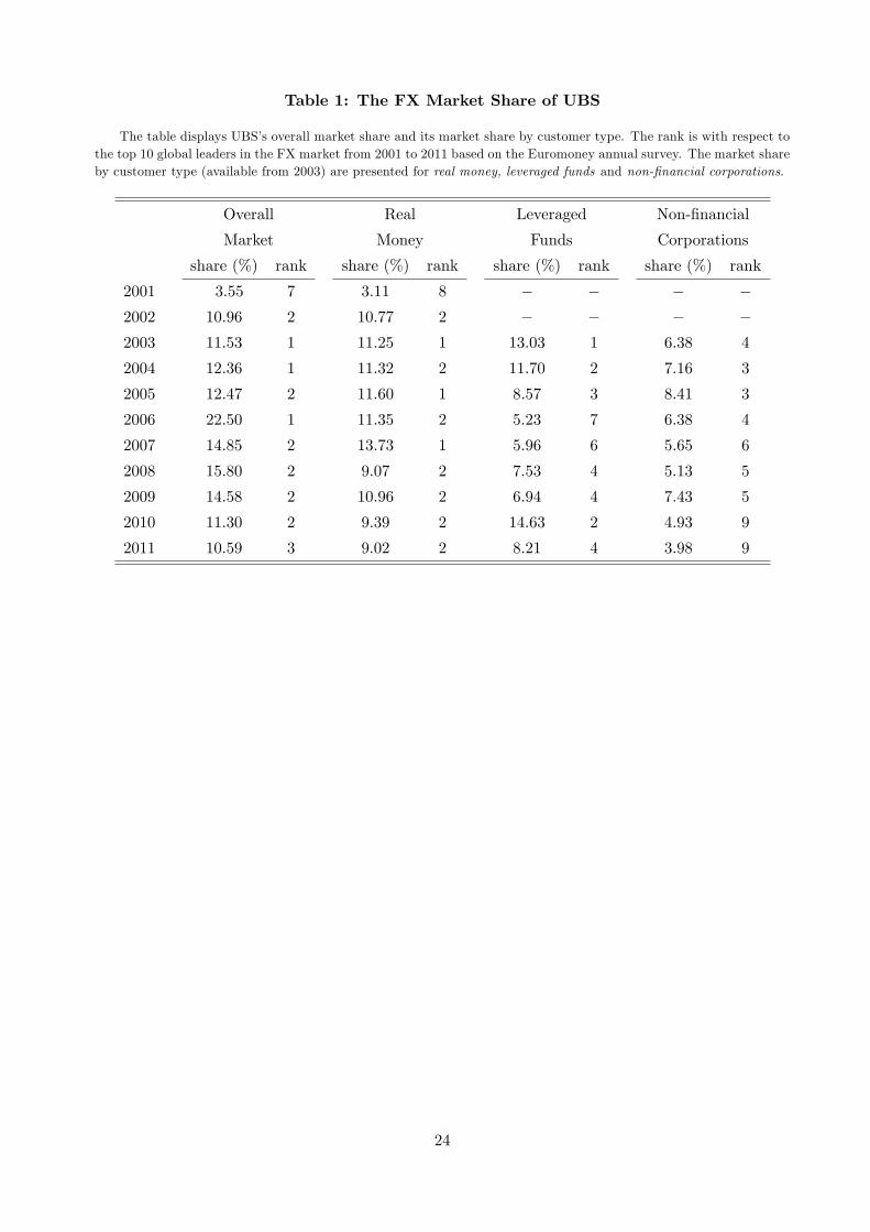
Table 1: The FX Market Share of UBS

The table displays UBS’s overall market share and its market share by customer type. The rank is with respect tothe top 10 global leaders in the FX market from 2001 to 2011 based on the Euromoney annual survey. The market shareby customer type (available from 2003) are presented for real money, leveraged funds and non-financial corporations.

Overall Real Leveraged Non-financial

Market Money Funds Corporations

share (%) rank share (%) rank share (%) rank share (%) rank

2001 3.55 7 3.11 8 − − − −2002 10.96 2 10.77 2 − − − −2003 11.53 1 11.25 1 13.03 1 6.38 4

2004 12.36 1 11.32 2 11.70 2 7.16 3

2005 12.47 2 11.60 1 8.57 3 8.41 3

2006 22.50 1 11.35 2 5.23 7 6.38 4

2007 14.85 2 13.73 1 5.96 6 5.65 6

2008 15.80 2 9.07 2 7.53 4 5.13 5

2009 14.58 2 10.96 2 6.94 4 7.43 5

2010 11.30 2 9.39 2 14.63 2 4.93 9

2011 10.59 3 9.02 2 8.21 4 3.98 9

24

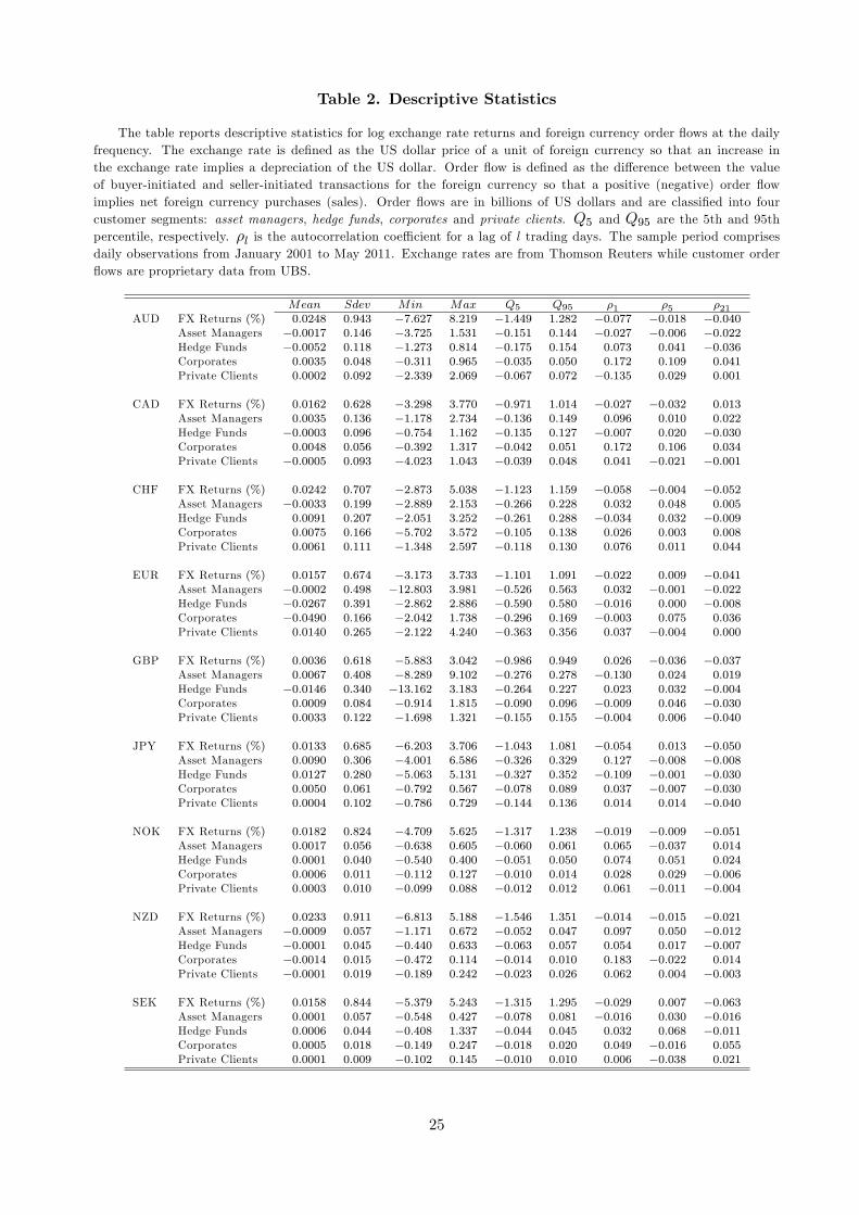
Table 2. Descriptive Statistics

The table reports descriptive statistics for log exchange rate returns and foreign currency order flows at the dailyfrequency. The exchange rate is defined as the US dollar price of a unit of foreign currency so that an increase inthe exchange rate implies a depreciation of the US dollar. Order flow is defined as the difference between the valueof buyer-initiated and seller-initiated transactions for the foreign currency so that a positive (negative) order flowimplies net foreign currency purchases (sales). Order flows are in billions of US dollars and are classified into fourcustomer segments: asset managers, hedge funds, corporates and private clients. Q5 and Q95 are the 5th and 95thpercentile, respectively. ρl is the autocorrelation coeffi cient for a lag of l trading days. The sample period comprisesdaily observations from January 2001 to May 2011. Exchange rates are from Thomson Reuters while customer orderflows are proprietary data from UBS.

Mean Sdev Min Max Q5 Q95 ρ1 ρ5 ρ21AUD FX Returns (%) 0.0248 0.943 −7.627 8.219 −1.449 1.282 −0.077 −0.018 −0.040

Asset Managers −0.0017 0.146 −3.725 1.531 −0.151 0.144 −0.027 −0.006 −0.022Hedge Funds −0.0052 0.118 −1.273 0.814 −0.175 0.154 0.073 0.041 −0.036Corporates 0.0035 0.048 −0.311 0.965 −0.035 0.050 0.172 0.109 0.041Private Clients 0.0002 0.092 −2.339 2.069 −0.067 0.072 −0.135 0.029 0.001

CAD FX Returns (%) 0.0162 0.628 −3.298 3.770 −0.971 1.014 −0.027 −0.032 0.013Asset Managers 0.0035 0.136 −1.178 2.734 −0.136 0.149 0.096 0.010 0.022Hedge Funds −0.0003 0.096 −0.754 1.162 −0.135 0.127 −0.007 0.020 −0.030Corporates 0.0048 0.056 −0.392 1.317 −0.042 0.051 0.172 0.106 0.034Private Clients −0.0005 0.093 −4.023 1.043 −0.039 0.048 0.041 −0.021 −0.001

CHF FX Returns (%) 0.0242 0.707 −2.873 5.038 −1.123 1.159 −0.058 −0.004 −0.052Asset Managers −0.0033 0.199 −2.889 2.153 −0.266 0.228 0.032 0.048 0.005Hedge Funds 0.0091 0.207 −2.051 3.252 −0.261 0.288 −0.034 0.032 −0.009Corporates 0.0075 0.166 −5.702 3.572 −0.105 0.138 0.026 0.003 0.008Private Clients 0.0061 0.111 −1.348 2.597 −0.118 0.130 0.076 0.011 0.044

EUR FX Returns (%) 0.0157 0.674 −3.173 3.733 −1.101 1.091 −0.022 0.009 −0.041Asset Managers −0.0002 0.498 −12.803 3.981 −0.526 0.563 0.032 −0.001 −0.022Hedge Funds −0.0267 0.391 −2.862 2.886 −0.590 0.580 −0.016 0.000 −0.008Corporates −0.0490 0.166 −2.042 1.738 −0.296 0.169 −0.003 0.075 0.036Private Clients 0.0140 0.265 −2.122 4.240 −0.363 0.356 0.037 −0.004 0.000

GBP FX Returns (%) 0.0036 0.618 −5.883 3.042 −0.986 0.949 0.026 −0.036 −0.037Asset Managers 0.0067 0.408 −8.289 9.102 −0.276 0.278 −0.130 0.024 0.019Hedge Funds −0.0146 0.340 −13.162 3.183 −0.264 0.227 0.023 0.032 −0.004Corporates 0.0009 0.084 −0.914 1.815 −0.090 0.096 −0.009 0.046 −0.030Private Clients 0.0033 0.122 −1.698 1.321 −0.155 0.155 −0.004 0.006 −0.040

JPY FX Returns (%) 0.0133 0.685 −6.203 3.706 −1.043 1.081 −0.054 0.013 −0.050Asset Managers 0.0090 0.306 −4.001 6.586 −0.326 0.329 0.127 −0.008 −0.008Hedge Funds 0.0127 0.280 −5.063 5.131 −0.327 0.352 −0.109 −0.001 −0.030Corporates 0.0050 0.061 −0.792 0.567 −0.078 0.089 0.037 −0.007 −0.030Private Clients 0.0004 0.102 −0.786 0.729 −0.144 0.136 0.014 0.014 −0.040

NOK FX Returns (%) 0.0182 0.824 −4.709 5.625 −1.317 1.238 −0.019 −0.009 −0.051Asset Managers 0.0017 0.056 −0.638 0.605 −0.060 0.061 0.065 −0.037 0.014Hedge Funds 0.0001 0.040 −0.540 0.400 −0.051 0.050 0.074 0.051 0.024Corporates 0.0006 0.011 −0.112 0.127 −0.010 0.014 0.028 0.029 −0.006Private Clients 0.0003 0.010 −0.099 0.088 −0.012 0.012 0.061 −0.011 −0.004

NZD FX Returns (%) 0.0233 0.911 −6.813 5.188 −1.546 1.351 −0.014 −0.015 −0.021Asset Managers −0.0009 0.057 −1.171 0.672 −0.052 0.047 0.097 0.050 −0.012Hedge Funds −0.0001 0.045 −0.440 0.633 −0.063 0.057 0.054 0.017 −0.007Corporates −0.0014 0.015 −0.472 0.114 −0.014 0.010 0.183 −0.022 0.014Private Clients −0.0001 0.019 −0.189 0.242 −0.023 0.026 0.062 0.004 −0.003

SEK FX Returns (%) 0.0158 0.844 −5.379 5.243 −1.315 1.295 −0.029 0.007 −0.063Asset Managers 0.0001 0.057 −0.548 0.427 −0.078 0.081 −0.016 0.030 −0.016Hedge Funds 0.0006 0.044 −0.408 1.337 −0.044 0.045 0.032 0.068 −0.011Corporates 0.0005 0.018 −0.149 0.247 −0.018 0.020 0.049 −0.016 0.055Private Clients 0.0001 0.009 −0.102 0.145 −0.010 0.010 0.006 −0.038 0.021

25

Table 3. Cross-Correlations

The table reports the cross-correlations among the daily log exchange rate returns and foreign currency order flows.The exchange rate is defined as the US dollar price of a unit of foreign currency so that an increase in the exchangerate implies a depreciation of the US dollar. Order flow is defined as the difference between the value of buyer-initiatedand seller-initiated transactions for the foreign currency so that a positive (negative) order flow implies net foreigncurrency purchases (sales). Order flows are in billions of US dollars and classified into four customer segments: assetmanagers, hedge funds, corporates and private clients. The superscripts a, b, and c denote statistical significance atthe 10%, 5%, and 1% level, respectively. The sample period comprises daily observations from January 2001 to May2011. Exchange rates are from Thomson Reuters while customer order flows are proprietary data from UBS.

FX Asset Hedge Corporates PrivateReturns Managers Funds Clients

AUD FX Returns 1.000Asset Managers 0.061c 1.000Hedge Funds 0.200c −0.048c 1.000Corporates −0.044b −0.008 −0.045b 1.000Private Clients −0.051c −0.094c −0.087c 0.022 1.000

CAD FX Returns 1.000Asset Managers 0.106c 1.000Hedge Funds 0.203c 0.010 1.000Corporates −0.047c −0.071c −0.005 1.000Private Clients −0.092c −0.205c −0.225c −0.046b 1.000

CHF FX Returns 1.000Asset Managers 0.149c 1.000Hedge Funds 0.312c 0.003 1.000Corporates −0.072c −0.175c −0.041b 1.000Private Clients −0.243c 0.023 −0.110c 0.047b 1.000

EUR FX Returns 1.000Asset Managers 0.049c 1.000Hedge Funds 0.130c −0.186b 1.000Corporates −0.056c 0.038b −0.016c 1.000Private Clients −0.348c −0.146 −0.027c 0.010c 1.000

GBP FX Returns 1.000Asset Managers 0.075c 1.000Hedge Funds 0.336c −0.039c 1.000Corporates −0.079c −0.043b −0.089 1.000Private Clients −0.344c −0.007c −0.170 0.121 1.000

JPY FX Returns 1.000Asset Managers 0.103c 1.000Hedge Funds 0.227c 0.022 1.000Corporates −0.050c −0.020 −0.009 1.000Private Clients −0.283c −0.115c −0.181c 0.103c 1.000

NOK FX Returns 1.000Asset Managers 0.068c 1.000Hedge Funds 0.083c 0.011 1.000Corporates −0.030 −0.073c −0.074c 1.000Private Clients 0.147c 0.016 0.048b −0.118c 1.000

NZD FX Returns 1.000Asset Managers 0.114c 1.000Hedge Funds 0.132 −0.077c 1.000Corporates 0.013 −0.017 0.070c 1.000Private Clients −0.014 −0.072c −0.023 0.036a 1.000

SEK FX Returns 1.000Asset Managers 0.103c 1.000Hedge Funds 0.065c −0.079c 1.000Corporates −0.007 −0.049c −0.027 1.000Private Clients 0.086c 0.032a 0.066c −0.078c 1.000

26

Table 4. The Predictive Ability of Daily Order Flows

The table shows the in-sample and out-of-sample performance of currency strategies investing in the G-10 developed

countries with daily rebalancing. The benchmark strategy is the naïve random walk (RW) model. The competing

strategies condition on lagged foreign currency order flow which is defined as the difference between the value of

buyer-initiated and seller-initiated transactions. Order flows are classified into four customer segments: asset managers

(AM), hedge funds (HF), corporates (CO) and private clients (PC). TOT indicates a strategy that conditions on total

(aggregate) customer order flows. ALL is a strategy that conditions on all four (disaggregated) customer order flows.

Using the exchange rate forecasts from each model, a US investor builds a maximum expected return strategy subject

to a target volatility σ∗p= 10% and proportional transaction costs. The strategy invests in a domestic bond and nine

foreign bonds and is rebalanced daily. For each strategy, we report the annualized mean (rp), annualized volatility(σp), skewness (Skew ), excess kurtosis (Kurt), annualized Sharpe ratio (SR), annualized Sortino ratio (SO), maximumdrawdown (MDD), and annualized performance fee (P) a risk-averse investor is willing to pay to switch from the

benchmark strategy to a competing strategy. For Skew and Kurt, we report both standard and robust measures to

outliers as in Kim and White (2004). For SR and SO, we report both standard and robust measures to serial correlation

as in Lo (2002). P is computed for γ = 6 and is expressed in annual basis points. The results are reported net of theeffective bid-ask spread, which is assumed to be equal to 50% of the quoted spread. The in-sample period comprises

daily observations from January 2001 to May 2011. The out-of-sample analysis runs from January 2004 to May 2011.

Exchange rates are from Thomson Reuters while customer order flows are proprietary data from UBS.

rp σp Skew Kurt SR SO MDD PStrategy (%) (%) std. rob. std. rob. std. rob. std. rob. (%) (bps)

In-Sample Period: Jan 2001 - May 2011

RW 2.9 9.6 −0.73 −0.06 11.11 1.17 0.13 0.13 0.16 0.15 37.0

AM 8.5 10.8 −0.20 −0.03 6.03 0.62 0.63 0.77 0.87 1.05 19.6 484

HF 11.1 9.9 0.05 −0.01 2.22 0.47 0.95 0.96 1.45 1.46 14.7 804

CO 10.7 10.3 −0.18 −0.02 2.12 0.48 0.88 0.95 1.29 1.41 17.1 736

PC 9.0 10.2 −0.24 −0.02 2.43 0.54 0.72 0.81 1.05 1.18 22.2 570

TOT 9.1 10.3 −0.09 −0.03 3.19 0.60 0.73 0.81 1.05 1.17 19.9 583

ALL 12.1 10.5 −0.19 0.00 2.75 0.61 1.00 1.25 1.44 1.79 14.0 871

Out-of-Sample Period: Jan 2004 - May 2011

RW −0.8 14.4 −0.72 −0.06 7.54 1.13 −0.17 −0.16 −0.20 −0.19 47.6

AM 0.9 13.1 −0.52 −0.06 2.22 0.96 −0.06 −0.05 −0.08 −0.07 38.8 279

HF 4.9 12.3 −0.45 −0.04 1.96 0.69 0.26 0.22 0.36 0.29 37.9 744

CO 4.1 13.8 −0.58 −0.06 2.68 0.86 0.18 0.16 0.23 0.20 39.7 549

PC 6.8 13.5 −0.57 −0.06 2.54 0.93 0.38 0.38 0.50 0.50 35.5 841

TOT 3.8 12.7 −0.55 −0.06 2.67 0.84 0.17 0.15 0.22 0.20 35.3 600

ALL 4.5 12.1 −0.52 −0.04 2.82 0.64 0.23 0.20 0.32 0.26 38.6 717

27

Table 5. The Predictive Ability of Monthly Order Flows

The table shows the in-sample and out-of-sample performance of currency strategies investing in the G-10 developed

countries with monthly rebalancing. The benchmark strategy is the naïve random walk (RW) model. The competing

strategies condition on lagged foreign currency order flow which is defined as the difference between the value of

buyer-initiated and seller-initiated transactions. Order flows are classified into four customer segments: asset managers

(AM), hedge funds (HF), corporates (CO) and private clients (PC). TOT indicates a strategy that conditions on total

(aggregate) customer order flows. ALL is a strategy that conditions on all four (disaggregated) customer order flows.

Using the exchange rate forecasts from each model, a US investor builds a maximum expected return strategy subject

to a target volatility σ∗p= 10% and proportional transaction costs. The strategy invests in a domestic bond and nine

foreign bonds and is rebalanced daily. For each strategy, we report the annualized mean (rp), annualized volatility(σp), skewness (Skew ), excess kurtosis (Kurt), annualized Sharpe ratio (SR), annualized Sortino ratio (SO), maximumdrawdown (MDD), and annualized performance fee (P) a risk-averse investor is willing to pay to switch from the

benchmark strategy to a competing strategy. For Skew and Kurt, we report both standard and robust measures to

outliers as in Kim and White (2004). For SR and SO, we report both standard and robust measures to serial correlation

as in Lo (2002). P is computed for γ = 6 and is expressed in annual basis points. The results are reported net of theeffective bid-ask spread, which is assumed to be equal to 50% of the quoted spread. The in-sample period comprises

monthly (non-overlapping) observations from January 2001 to May 2011. The out-of-sample analysis runs from January

2004 to May 2011. Exchange rates are from Thomson Reuters while customer order flows are proprietary data from

UBS.

rp σp Skew Kurt SR SO MDD PStrategy (%) (%) std. rob. std. rob. std. rob. std. rob. (%) (bps)

In-Sample Period: Jan 2001 - May 2011

RW 9.4 10.0 −0.26 0.02 0.04 0.12 0.70 0.58 1.11 0.92 −28.0AM 14.6 10.3 0.18 −0.05 1.68 1.50 1.18 0.96 1.91 1.55 −12.6 504

HF 15.5 9.6 0.11 −0.02 0.52 0.55 1.35 1.21 2.44 2.18 −9.2 626

CO 17.3 9.7 0.15 0.03 0.33 0.54 1.53 1.97 2.82 3.63 −5.6 806

PC 11.4 9.4 −0.39 −0.07 0.88 0.91 0.95 0.74 1.41 1.10 −17.3 229

TOT 15.0 10.4 0.21 −0.01 2.27 3.19 1.21 1.03 1.75 1.49 −11.1 539

ALL 19.5 10.5 0.38 0.10 0.87 0.79 1.63 1.26 3.07 2.37 −9.8 983

Out-of-Sample Period: Jan 2004 - May 2011

RW 5.2 13.4 −0.28 0.02 0.53 0.54 0.20 0.17 0.31 0.26 −40.2AM 13.3 12.9 0.05 0.01 0.57 0.07 0.84 0.74 1.45 1.28 −21.1 877

HF 10.5 13.0 −0.28 −0.12 0.61 1.21 0.61 0.57 0.92 0.85 −29.9 561

CO 10.4 15.4 −0.24 0.04 0.50 0.34 0.51 0.53 0.80 0.83 −33.0 343

PC −5.0 17.2 −1.54 −0.11 4.56 3.40 −0.44 −0.27 −0.46 −0.28 −65.1 −1587TOT 7.8 13.7 −1.21 −0.09 3.19 1.46 0.38 0.43 0.44 0.49 −28.4 180

ALL 13.1 13.5 −0.06 −0.03 1.02 0.81 0.79 0.76 1.22 1.18 −23.9 800

28

Table 6. Daily Order Flows and Macroeconomic Information

The table displays the estimates of the following regressions(rsp,t − rf,t

)= α+

∑i βi(rip,t − rf,t

)+εt, where

rp,t is the portfolio return of a currency strategy investing in the G-10 developed countries with daily rebalancing andrf,t is the daily riskless return. r

sp,t indicates a strategy conditioning on the currency order flows of asset managers

(AM ), corporates (CO), hedge funds (HF ), and private clients (PC ), respectively. rip,t refers to a strategy using therandom walk (RW), forward premium (FP), purchasing power parity (PPP), monetary fundamentals (MF), Taylor rule

(TR), cyclical external imbalances (NXA) and momentum (MOM), respectively. The portfolio returns are computed

net of the effective bid-ask spread, which is assumed to be equal to 50% of the quoted spread. The superscripts a,

b, and c denote statistical significance at the 10%, 5%, and 1% level, respectively. Bootstrapped standard errors (in

parentheses) and p-values are obtained by resampling 10,000 times the portfolio weights by means of moving block

bootstrap (see Gonçalves and White, 2005). The portfolio returns run from January 2001 to May 2011. Exchange

rates are from Thomson Reuters while customer order flows are proprietary data from UBS. All other data are from

Datastream, OECD and IFS.

α βRW βFP βTR βPPP βMF βNXA βMOM R2(%)

In-Sample Period: Jan 2001 - May 2011AM −0.022 0.271c 0.045a 0.315c 0.517c −0.059b 62.1

(0.021) (0.027) (0.025) (0.035) (0.047) (0.026) (1.60)

−0.035 0.297c 0.018 0.245c 0.435c −0.134c 61.0(0.022) (0.032) (0.027) (0.039) (0.049) (0.030) (2.00)

−0.044b 0.254c 0.001 0.187c 0.560c −0.057b 60.6(0.021) (0.025) (0.025) (0.037) (0.046) (0.029) (1.80)

−0.041b 0.206c 0.225c 0.153c 0.056b 0.225c 0.361c −0.048a 66.1(0.020) (0.026) (0.031) (0.025) (0.023) (0.037) (0.042) (0.024) (1.60)

HF 0.014 0.202c 0.102c 0.373c 0.363c 0.037b 66.9(0.018) (0.019) (0.024) (0.032) (0.033) (0.016) (1.40)

0.003 0.246c 0.083c 0.318c 0.286c −0.021 66.8(0.019) (0.032) (0.026) (0.036) (0.043) (0.018) (2.00)

−0.002 0.175c 0.067c 0.283c 0.399c 0.035a 65.5(0.018) (0.021) (0.024) (0.036) (0.034) (0.017) (1.60)

0.001 0.155c 0.197c 0.094c 0.112c 0.310c 0.233c 0.039b 69.8(0.017) (0.022) (0.032) (0.022) (0.024) (0.036) (0.038) (0.018) (1.60)

CO 0.009 0.187c 0.132c 0.337c 0.415c 0.045b 67.5(0.018) (0.021) (0.022) (0.025) (0.033) (0.017) (1.60)

0.001 0.204c 0.113c 0.289c 0.359c −0.007 66.9(0.018) (0.028) (0.023) (0.028) (0.038) (0.021) (1.90)

−0.011 0.239c 0.102c 0.226c 0.429c 0.061c 68.3(0.018) (0.022) (0.022) (0.030) (0.034) (0.019) (1.80)

−0.009 0.127c 0.142c 0.175c 0.137c 0.249c 0.304c 0.067c 70.7(0.017) (0.023) (0.027) (0.022) (0.022) (0.030) (0.036) (0.018) (1.60)

PC −0.017 0.178c 0.072c 0.433c 0.390c 0.021 71.0(0.017) (0.019) (0.021) (0.029) (0.028) (0.014) (1.40)

−0.029 0.300c 0.063c 0.375c 0.270c −0.034b 73.2(0.017) (0.024) (0.022) (0.032) (0.038) (0.015) (1.50)

−0.030a 0.146c 0.042b 0.357c 0.424c 0.017 69.9(0.017) (0.019) (0.021) (0.032) (0.029) (0.017) (1.40)

−0.030a 0.131c 0.262c 0.060c 0.087c 0.375c 0.227c 0.011 75.0(0.016) (0.019) (0.024) (0.020) (0.021) (0.033) (0.034) (0.015) (1.30)

Continued

29

Table 7. Daily Order Flows and Combined Forecasting Strategies

The table displays the estimates of the following regressions(rsp,t − rf,t

)= α + βi

(rip,t − rf,t

)+ εt where

rp,t is the portfolio return of a currency strategy investing in the G-10 developed countries with daily rebalancing andrf,t is the daily riskless return. r

sp,t indicates a strategy conditioning on the currency order flows of Asset Managers

(AM ), corporates (CO), hedge funds (HF ), and private clients (PC ). rip,t refers to a strategy that combines the randomwalk (RW), forward premium (FP), purchasing power parity (PPP), monetary fundamentals (MF), Taylor rule (TR),

cyclical external imbalances (NXA) and momentum (MOM). The combination employs the average (AVE ), median

(MED), trimmed mean (TRI ), and mean-squared error (MSE ) of the forecasts, the “kitchen sink”(KS) regression that

incorporates all predictors into a multiple predictive regression, and the “Fund of Funds”(FoF) strategy that equally

invests in the underlying portfolio strategies. The portfolio returns are computed net of the effective bid-ask spread,

which is assumed to be equal to 50% of the quoted spread. The superscripts a, b, and c denote statistical significance

at the 10%, 5%, and 1% level, respectively. Bootstrapped standard errors (in parentheses) and p-values are obtained

by resampling 10,000 times the portfolio weights by means of moving block bootstrap (see Gonçalves and White, 2005).

The portfolio returns run from January 2001 to May 2011. Exchange rates are from Thomson Reuters while customer

order flows are proprietary data from UBS. All other data are from Datastream, OECD and IFS.

α β R2(%) α β R

2(%) α β R

2(%)

AV E MED TRI

AM −0.019 0.732c 48.5 −0.027 0.796c 56.6 −0.045b 0.849c 60.9(0.024) (0.027) (3.30) (0.023) (0.024) (2.50) (0.021) (0.02) (2.00)

CO 0.006 0.741c 58.9 0.005 0.746c 58.9 −0.015 0.818c 66.9(0.019) (0.023) (2.10) (0.02) (0.023) (2.80) (0.018) (0.019) (2.00)

HF −0.001 0.763c 57.7 −0.007 0.811c 64.4 −0.024 0.857c 67.9(0.021) (0.025) (2.50) (0.019) (0.02) (2.10) (0.018) (0.019) (1.90)

PC −0.021 0.792c 63.2 −0.025 0.822c 67.0 −0.044c 0.876c 72.0(0.019) (0.018) (1.80) (0.019) (0.018) (2.30) (0.017) (0.014) (1.50)

MSE KS FoF

AM −0.019 0.733c 48.5 0.084b −0.162c 2.4 −0.016 1.24c 58.4(0.024) (0.027) (3.40) (0.033) (0.034) (1.00) (0.022) (0.032) (2.00)

CO 0.006 0.744c 59.2 0.107c −0.128c 1.8 0.012 1.216c 66.6(0.019) (0.023) (2.10) (0.031) (0.026) (0.80) (0.018) (0.028) (1.30)

HF −0.001 0.764c 57.7 0.097c −0.071b 0.4 0.003 1.283c 68.5(0.021) (0.025) (2.50) (0.032) (0.03) (0.50) (0.018) (0.022) (1.60)

PC −0.021 0.794c 63.3 0.086c −0.128c 1.6 −0.014 1.28c 69.3(0.019) (0.018) (1.80) (0.032) (0.03) (0.80) (0.018) (0.021) (1.30)

30

Figure 1. Contemporaneous Correlation of Currency Flows and Returns

This figure shows the correlation coefficient between the contemporaneous customer order flows and exchange rate returns for different horizons. The correlation is the average

across nine US dollar nominal exchange rates. The horizon is measured in days and shown in log-scale. The blue line is the in sample panel correlation coefficient computed

using overlapping return windows from 1 (100) to 252 (> 102) trading days, while the red lines represent the 90th percentile bootstrap confidence intervals generating by 10,000

replications. Order flows are shown for four customer segments: asset managers, hedge funds, corporates and private clients. The sample period comprises daily data from

January 2001 to May 2011. Exchange rates are from Thomson Reuters while customer order flows are proprietary data from UBS.

31

Figure 2. Daily Cumulative Wealth of Currency Flow Strategies

This figure displays the cumulative wealth of out-of-sample currency strategies investing in the G-10 developed countries with daily rebalancing. The blue line represents the

benchmark strategy based on the naıve random walk model. The red line indicates a strategy conditioning on order flow for one of four customer segments: asset managers,

hedge funds, corporates and private clients. Initial wealth is $1 growing at the portfolio return, net of transaction costs. The out-of-sample analysis runs from January 2004 to

May 2011. Exchange rates are from Thomson Reuters while customer order flows are proprietary data from UBS.

32

Figure 3. Rolling Estimates: the Alphas

The figure displays the one-year rolling estimate of α (solid line) and its 95% confidence interval (dashed lines) for the regression (rsp,t− rf ) = α+∑

i βi(rip,t− rf ) + εt, where rp,t

is the portfolio return, net of transaction costs, of a currency strategy investing in the G-10 developed countries with daily rebalancing, and rf is the riskless return. s indicates

a strategy conditioning on the currency order flow of asset managers (AM), hedge funds (HF), corporates (CO) and private clients (PC). i refers to the random walk (RW),

forward premium (FP), Taylor rule (TR), purchasing power parity (PPP), monetary fundamentals (MF), cyclical external imbalances (NXA) and momentum (MOM) strategy.

The sample analysis runs from January 2001 to May 2011. Exchange rates are from Thomson Reuters while customer order flows are proprietary data from UBS.

33

Figure 4. Rolling Estimates: Asset Managers

The figure displays the one-year rolling estimates of βi for the regression (rAMp,t − rf ) = α+

∑i βi(r

ip,t − rf ) + εt where rp,t is the portfolio return, net of transaction costs, of a

currency strategy investing in the G-10 developed countries with daily rebalancing, and rf is the riskless return. AM denotes a strategy conditioning on the currency order flow

of asset managers. i refers to the random walk (RW), forward premium (FP), Taylor rule (TR), purchasing power parity (PPP), monetary fundamentals (MF), cyclical external

imbalances (NXA) and momentum (MOM) strategy. The sample analysis runs from January 2001 to May 2011. Exchange rates are from Thomson Reuters while customer order

flows are proprietary data from UBS.

34

Figure 5. Rolling Estimates: Hedge Funds

The figure displays the one-year rolling estimates of βi for the regression (rHFp,t − rf ) = α +

∑i βi(r

ip,t − rf ) + εt where rp,t is the portfolio return, net of transaction costs, of

a currency strategy investing in the G-10 developed countries with daily rebalancing, and rf is gross riskless return. HF denotes a strategy conditioning on the currency order

flow of hedge funds. i refers to the random walk (RW), forward premium (FP), Taylor rule (TR), purchasing power parity (PPP), monetary fundamentals (MF), cyclical external

imbalances (NXA) and momentum (MOM) strategy. The sample analysis runs from January 2001 to May 2011. Exchange rates are from Thomson Reuters while customer order

flows are proprietary data from UBS.

35

Figure 6. Rolling Estimates: Corporates

The figure displays the one-year rolling estimates of βi for the regression (rCOp,t − rf ) = α +

∑i βi(r

ip,t − rf ) + εt where rp,t is the portfolio return, net of transaction costs, of

a currency strategy investing in the G-10 developed countries with daily rebalancing, and rf is the riskless return. CO denotes a strategy conditioning on the currency order

flow of corporates. i refers to the random walk (RW), forward premium (FP), Taylor rule (TR), purchasing power parity (PPP), monetary fundamentals (MF), cyclical external

imbalances (NXA) and momentum (MOM) strategy. The sample analysis runs from January 2001 to May 2011. Exchange rates are from Thomson Reuters while customer order

flows are proprietary data from UBS.

36

Figure 7. Rolling Estimates: Private Clients

The figure displays the one-year rolling estimates of βi for the regression (rPCp,t − rf ) = α +

∑i βi(r

ip,t − rf ) + εt where rp,t is the portfolio return, net of transaction costs, of

a currency strategy investing in the G-10 developed countries with daily rebalancing, and rf is the gross riskless return. PC denotes a strategy conditioning on the currency

order flow of private clients. i refers to the random walk (RW), forward premium (FP), Taylor rule (TR), purchasing power parity (PPP), monetary fundamentals (MF), cyclical

external imbalances (NXA) and momentum (MOM) strategy. The sample analysis runs from January 2001 to May 2011. Exchange rates are from Thomson Reuters while

customer order flows are proprietary data from UBS.

37

References

Akram, F., D. Rime, and L. Sarno (2008). “Arbitrage in the Foreign Exchange Market: Turning onthe Microscope,”Journal of International Economics 76, 237—253.

Bjonnes, G., and D. Rime (2005). “Dealer Behaviour and Trading Systems in the Foreign ExchangeMarkets,”Journal of Financial Economics 75, 571—605.

Burnside, C., M. Eichenbaum, I. Kleshchelski, and S. Rebelo (2011). “Do Peso Problems Explainthe Returns to the Carry Trade?”Review of Financial Studies 24, 853—891.

Bacchetta, P., and E. van Wincoop (2004). “A Scapegoat Model of Exchange-Rate Fluctuations?”American Economic Review Papers and Proceedings 94, 114—118.

Bacchetta, P., and E. van Wincoop (2006). “Can Information Heterogeneity Explain the ExchangeRate Determination Puzzle?”American Economic Review 96, 552—576.

Bates, J.M., and C.W.J. Granger (1969). “The Combination of Forecasts,” Operations ResearchQuarterly 20, 451—468.

Berger, D.W., A.P. Chaboud, S.V. Chernenko, E. Howorka, and J.H. Wright (2008). “Order Flow andExchange Rate Dynamics in Electronic Brokerage System Data,”Journal of International Economics75, 93—109.

Bilson, J.F.O. (1981). “The ‘Speculative Effi ciency’Hypothesis,”Journal of Business 54, 435—451.

Daníelsson, J., J. Luo, and R. Payne (2011). “Exchange Rate Determination and Inter-Market OrderFlow Effects,”European Journal of Finance, forthcoming.

Cerrato, M., N. Sarantis, and A. Saunders (2011). “An Investigation of Customer Order Flow in theForeign Exchange Market,”Journal of Banking and Finance 35, 1892—1906.

Cheung, Y.-W., and M.D. Chinn (2001). “Currency Traders and Exchange Rate Dynamics: A Surveyof the US Market,”Journal of International Money and Finance 20, 439—471,

Della Corte, P., L. Sarno, and G. Sestieri (2010). “The Predictive Information Content of ExternalImbalances for Exchange Rate Returns: How Much Is It Worth?,”Review of Economics and Statistics(forthcoming).

Della Corte, P., L. Sarno, and I. Tsiakas (2009). “An Economic Evaluation of Empirical ExchangeRate Models.”Review of Financial Studies 22, 3491—3530.

Easley, D., and M. O’Hara (1992). “Adverse Selection and Large Trade Volume: The Implicationsfor Market Effi ciency,”Journal of Financial and Quantitative Analysis 27, 185—208.

Engel, C., N.C. Mark, and K.D. West (2008). “Exchange Rate Models Are Not as Bad as YouThink,” in Acemoglu, D., Rogoff, K., and Woodford, M. (eds.), NBER Macroeconomics Annual2007. Cambridge, MA: MIT Press, 381—441.

Engel, C., and K.D. West (2005). “Exchange Rates and Fundamentals,”Journal of Political Economy113, 485—517.

Evans, M.D.D. (2010). “Order Flows and the Exchange Rate Disconnect Puzzle,”Journal of Inter-national Economics 80, 58—71.

Evans, M.D.D. (2011). Exchange-Rate Dynamics, Princeton: Princeton University Press.

38

Evans, M.D.D., and R.K. Lyons (2002). “Order Flow and Exchange Rate Dynamics,” Journal ofPolitical Economy 110, 170—180.

Evans, M.D.D., and R.K. Lyons (2005). “Meese-Rogoff Redux: Micro-based Exchange Rate Fore-casting,”American Economic Review Papers and Proceedings 95, 405—414.

Evans, M.D.D., and R.K. Lyons (2006). “Understanding Order Flow” International Journal of Fi-nance and Economics 11, 2—23.

Evans, M.D.D., and R.K. Lyons (2007). “Exchange Rate Fundamentals and Order Flow,”Unpub-lished working paper, Georgetown University.

Evans, M.D.D., and R.K. Lyons (2008). “How Is Macro News Transmitted to Exchange Rates?”Journal of Financial Economics 88, 26—50.

Froot, K.A., and T. Ramadorai (2005). “Currency Returns, Intrinsic Value, and Institutional-InvestorFlows,”Journal of Finance 60, 1535—1566.

Glosten, L., and P. Milgrom (1985). “Bid, Ask, and Transaction Prices in a Specialist Market withHeterogeneously Informed Agents,”Journal of Financial Economics 14, 71—100.

Goetzmann, W., J. Ingersoll, M. Spiegel, and I. Welch (2007). “Portfolio Performance Manipulationand Manipulation-Proof Performance Measures,”Review of Financial Studies 20, 1503—1546.

Gonçalves, S., and H. White (2005). “Bootstrap Standard Error Estimates for Linear Regression,”Journal of the American Statistical Association 100, 970—979.

Goodhart, C.A.E. (1988). “The Foreign Exchange Market: A Random Walk with a Dragging An-chor,”Economica 55, 437—460.

Gourinchas, P.-O., and H. Rey (2007). “International Financial Adjustment,” Journal of PoliticalEconomy 115, 665—703.

Goyal, A., and A. Saretto (2009). “Cross-Section of Option Returns and Volatility,” Journal ofFinancial Economics 94, 310—326.

Gradojevic N., and C.J. Neely (2009). “The Dynamic Interaction of Order Flows and the CAD/USDExchange Rate,”Federal Reserve Bank of St. Louis working paper.

Groen, J.J.J. (2000). “The Monetary Exchange Rate Model as a Long-Run Phenomenon,”Journalof International Economics 52, 299—319.

Han, Y. (2006). “Asset Allocation with a High Dimensional Latent Factor Stochastic VolatilityModel,”Review of Financial Studies, 19, 237-271.

Hodrick, R.J., and E.C. Prescott (1997). “Postwar U.S. Business Cycles: An Empirical Investigation,”Journal of Money, Credit and Banking 29, 1—16.

Killeen, W.P., R.K. Lyons, and M.J. Moore (2006). “Fixed versus flexible: Lessons from EMS OrderFlow,”Journal of International Money and Finance 25, 551—579.

Kim, T-H., and H. White (2004). “On More Robust Estimation of Skewness and Kurtosis,”FinanceResearch Letters 1, 56—73.

Kyle, A.S. (1985). “Continuous Auctions and Insider Trading,”Econometrica 53, 1315—1335.

Lo, A.W. (2002). “The Statistics of Sharpe Ratios,”Financial Analysts Journal, 58, 36—52.

39

Lobo, M.S., M. Fazel, and S. Boyd (2007). “Portfolio Optimization with Linear and Fixed TransactionCosts,”Annals of Operations Research 152, 341—365.

Lustig, H., N. Roussanov, and A. Verdelhan (2011). “Common Risk Factors in Currency Markets,”Review of Financial Studies (forthcoming).

Lyons, R.K. (2001). The Microstructure Approach to Exchange Rates, Cambridge: MIT Press.

Mancini-Griffoli, T., and A. Ranaldo (2011). “Limits to Arbitrage during the Crisis: Funding Liq-uidity Constraints and Covered Interest Parity,”Swiss National Bank working paper 2010-14.

Mark, N.C. (1995). “Exchange Rates and Fundamentals: Evidence on Long-Horizon Predictability,”American Economic Review 85, 201—218.

Mark, N.C. (2009). “Changing Monetary Policy Rules, Learning, and Real Exchange Rate Dynam-ics,”Journal of Money, Credit and Banking 41, 1047—1070.

Marquering, W., and M. Verbeek (2004). “The Economic Value of Predicting Stock Index Returnsand Volatility,”Journal of Financial and Quantitative Analysis, 39, 407-429.

Marsh, I.W., and C. O’Rourke (2005). “Customer Order Flow and Exchange Rate Movements: IsThere Really Information Content?”Unpublished working paper, Cass Business School.

Meese, R.A., and K. Rogoff (1983). “Empirical Exchange Rate Models of the Seventies: Do TheyFit Out of Sample?”Journal of International Economics 14, 3—24.

Menkhoff, L., L. Sarno, M. Schmeling, and A. Schrimpf (2011). “Carry Trades and Global ForeignExchange Volatility,”Journal of Finance (forthcoming).

Molodtsova, T., and D.H. Papell (2009). “Out-of-Sample Exchange Rate Predictability with TaylorRule Fundamentals?”Journal of International Economics 77, 167—180.

Orphanides, A. (2001). “Monetary Policy Rules Based on Real-Time Data,”American EconomicReview 91, 964—985.

Orphanides, A., and S. van Norden (2002). “The Unreliability of Output Gap Estimates in RealTime,”Review of Economics and Statistics 84, 569—583.

Payne, R. (2003). “Informed Trade in Spot Foreign Exchange Markets: An Empirical Investigation,”Journal of International Economics 61, 307—329.

Pojarliev, M., and R.M. Levich (2008). “Do Professional Currency Managers Beat the Benchmark?”Financial Analysts Journal 64, 18—32.

Rapach, D.E., J.K. Strauss, and G. Zhou (2010). “Out-of-Sample Equity Premium Prediction: Com-bination Forecasts and Links to the Real Economy.”Review of Financial Studies 23, 821—862.

Rapach, D.E., and M.E. Wohar (2002). “Testing the Monetary Model of Exchange Rate Determina-tion: New Evidence from a Century of Data,”Journal of International Economics 58, 359—385.

Rime, D., L. Sarno, and E. Sojli (2010). “Exchange Rate Forecasting, Order Flow and MacroeconomicInformation,”Journal of International Economics 80, 72—88.

Rogoff, K.S. (1996). “The Purchasing Power Parity Puzzle,” Journal of Economic Literature 34,647—668.

40

Sager, M.J., and M.P. Taylor (2008). “Commercially Available Order Flow Data and Exchange RateMovements: Caveat Emptor,”Journal of Money, Credit and Banking 40, 583—625.

Sarno, L., and G. Valente (2009). “Exchange Rates and Fundamentals: Footloose or Evolving Rela-tionship?”Journal of the European Economic Association 7, 786—830.

Stock, J.H., and M.W.Watson (2004). “Combination Forecasts of Output Growth in a Seven-CountryData Set,”Journal of Forecasting 23, 405—430.

Taylor, J.B. (1993). “Discretion versus Policy Rules in Practice,” Carnegie-Rochester ConferenceSeries on Public Policy 39, 195—214.

Taylor, A.M., and M.P. Taylor (2004). “The Purchasing Power Parity Debate,”Journal of EconomicPerspectives 18, 135—158.

Timmermann, A. (2006). “Forecast Combinations,”in Elliott, G., C.W.J. Granger, and A. Timmer-mann (eds.), Handbook of Economic Forecasting, Amsterdam: Elsevier.

Welch, I., and A. Goyal (2008). “A Comprehensive Look at The Empirical Performance of EquityPremium Prediction,”Review of Financial Studies 21, 1455—1508.

41

Appendix A: Robust Regression

Daily order flow data may contain outliers. Standard least square estimates can behave badly when

the error distribution is not normal and heavy-tailed. Removing outliers from the sample is not

a meaningful solution as subjective outlier deletion or algorithms have the drawback of removing

legitimate observations. Instead, robust regression aims at obtaining parameter estimates that are

not adversely affected by the presence of potential outliers (Hampel, Ronchetti, Rousseeuw and

Stahel, 2005). The most common general method of robust regression is M-estimation introduced

by Huber (1964).

In brief, consider the following linear model:

yt = x′tβ + εt.

Robust parameter estimates are the solutions to:

minβ

T∑t=1

ρ

(yt − x′tβ

σ

), (16)

where σ is the scale of the error term, and ρ (·) is a bisquare function defined as:

ρ (y) =

1−

[1− (y/k)2

]3if |y| ≤ k

1 if |y| > k.

The first order condition for the optimization problem in Equation (16) is:

T∑t=1

ρ′

(yt − x′tβ

σ

)x′t = 0, (17)

where

ρ′ (y) =

6y/k2 −

[1− (y/k)2

]2if |y| ≤ k

0 if |y| > k.

is the derivative of ρ (·). In the bisquare function the constant k = 4.685 ensures 95% effi ciency of

β when errors are normal. Computationally, the parameters are found using iteratively reweighed

least squares with a weighting function corresponding to the bisquare function ρ (y) and an initial

estimate for the residual scale of σ = MAR/0.6745, where MAR is the median absolute residual.

While least-squares assign equal weight to each residual, the weights of the bisquare estimator decline

as soon as the residual departs from 0, and is 0 for |y| > k. Compared to standard least squares, by

construction, robust regression estimates are less influenced by potential contamination in the data

(Maronna, Martin and Yohai, 2006).

42

Appendix B: Contemporaneous Regressions between Exchange Ratesand Order Flow

We investigate the relation between exchange rates and order flow by estimating contemporaneous

regressions using ordinary least squares (OLS). For each exchange rate, we estimate three types of

regressions: (i) the excess FX return on each of the four types of order flow separately (individual

regressions); (ii) the excess FX return on the four types of order flow together in one regression

(disaggregated regressions); and (iii) the excess FX return on the single total order flow (aggregate

regressions). The results are presented in Table C3 for daily data and Table C4 for monthly data.21

For the daily results of individual regressions in Table C3, the order flow coeffi cients are always

positive for asset managers (AM) and hedge funds (HF), but tend to be negative for corporate clients

(CO) and private clients (PC). The positive sign for AM and HF implies that net buying pressure

of these customers for foreign currency is contemporaneously related to positive FX excess returns.

In other words, increased demand leads to positive return. Similarly, the negative sign for CO and

PC implies that net selling pressure of these customers for foreign currency is contemporaneously

related to negative FX excess returns. At first glance, the negative sign of some coeffi cients appears

counterintuitive. Evans and Lyons (2006, 2007) find similar results when using customer order flows

from Citibank for the euro-US dollar exchange rate. They argue that it is diffi cult to disentangle

liquidity-motivated order flow from informative order flow. Hence one interpretation is simply that

CO and PC may act as liquidity providers. They also show that individual coeffi cients have no

structural interpretation in terms of measuring the price impact of different customer orders, they

simply map variations in customer order flows into an estimate of the information flow being used by

dealers across the market.22 Note that the positive sign of the AM and HF betas is highly statistically

significant for all exchange rates (but one), whereas the negative sign of the CO and PC betas is

significant only for about half of the exchange rates. The R2revolves around 1% but can be as high

as 12% in the case of PC for GBP.

The results improve significantly when we move to the disaggregated regressions. Whereas the

21Note that Evans and Lyons (2002) and all their subsequent papers use FX returns rather than FX excess returnson the left hand side of these regressions. We report results for FX excess returns as this is the relevant quantityto predict in determining the weights for allocating wealth across international bonds. Note that the results remainqualitatively identical when using as the dependent variable either FX returns or FX excess returns (results availableupon request).22Evans and Lyons (2006, 2007) build a model where realized FX returns reflect the revision in dealer’s quotes

driven by new information concerning fundamentals. This information arrives in the form of public news, macroannouncements and inter-dealer order flow, but not the customer order flows of individual dealers.

43

sign and significance of the betas is similar to the individual regressions, the R2is much higher

ranging from about 3% to 20%. In other words, using the distinct information from all four order

flow types can substantially improve the explanatory power of order flow. We find further evidence

of this in the aggregate order flow regression, where the betas are positive and significant but the R2

is much lower than the disaggregated regression, revolving around 1%-2%.

Turning to Table C4, we find that the results for monthly data are qualitatively identical to those

for daily data. The one important difference is that the monthly R2is much higher than the daily

R2. For the disaggregated order flow, for example, the average R

2is about 16% and can be as high

as 30%. The monthly results confirm that the disaggregated order flow has superior explanatory

power than the total order flow.

In conclusion, this analysis provides strong evidence of a contemporaneous relation between FX

excess returns and customer flows, leading to two main conclusions. First, there is a positive relation

between AM and HF flows with FX excess returns and a negative relation for CO and PC flows.

Second, the inclusion of all four types of order flow separately in the contemporaneous regressions

provides the highest explanatory power.

44

Appendix C: Further Tables

Table C1: Top 10 Leaders in FX Market Share

The table displays the overall market share in annual turnover for the top 10 leaders in the foreign exchange (FX) market from 2001 to 2011. The data are collectedfrom the Euromoney annual survey of the global FX industry (Euromoney FX Survey).

FX Market in 2001 share (%) FX Market in 2002 share (%) FX Market in 2003 share (%) FX Market in 2004 share (%)1 Citigroup 974 Citigroup 1117 UBS 1153 UBS 1236

2 Deutsche Bank 908 UBS Warburg 1096 Citigroup 987 Deutsche Bank 1218

3 Goldman Sachs 709 Deutsche Bank 979 Deutsche Bank 979 Citigroup 937

4 JP Morgan 522 Goldman Sachs 669 JP Morgan Chase 679 JP Morgan 578

5 Chase Manhattan Bank 469 JP Morgan Chase 586 Goldman Sachs 556 HSBC 489

6 Credit Suisse First Boston 410 Credit Suisse First Boston 462 Credit Suisse First Boston 423 Goldman Sachs 454

7 UBS Warburg 355 Morgan Stanley 370 HSBC 389 Barclays Capital 408

8 State Street Bank & Trust 299 ABN Amro 340 Morgan Stanley 387 Credit Suisse First Boston 379

9 Bank of America 299 SEB 276 Barclays Capital 384 RBS 351

10 Morgan Stanley Dean Witter 287 Barclays Capital 261 ABN Amro 363 Merrill Lynch 349

FX Market in 2005 share (%) FX Market in 2006 share (%) FX Market in 2007 share (%) FX Market in 2008 share (%)1 Deutsche Bank 1672 UBS 2250 Deutsche Bank 1930 Deutsche Bank 2170

2 UBS 1247 Deutsche Bank 2006 UBS 1485 UBS 1580

3 Citigroup 750 Citigroup 1059 Citigroup 900 Barclays 912

4 HSBC 637 RBS 653 RBS 890 Citigroup 749

5 Barclays Capital 585 Barclays Capital 453 Barclays Capital 880 RBS 730

6 Merrill Lynch 569 Bank of America 386 Bank of America 529 JP Morgan 419

7 JP Morgan 529 HSBC 366 HSBC 436 HSBC 410

8 Goldman Sachs 439 JP Morgan 336 Goldman Sachs 414 Lehman Brothers 358

9 ABN Amro 419 Dresdner Kleinwort W. 254 JP Morgan 333 Goldman Sachs 347

10 Morgan Stanley 392 Goldman Sachs 250 Morgan Stanley 286 Morgan Stanley 256

FX Market in 2009 share (%) FX Market in 2010 share (%) FX Market in 2011 share (%)1 Deutsche Bank 2096 Deutsche Bank 1806 Deutsche Bank 1584

2 UBS 1458 UBS 1130 Barclays Capital 1075

3 Barclays Capital 1045 Barclays Capital 1108 UBS 1059

4 RBS 819 Citi 769 Citi 888

5 Citigroup 732 RBS 650 JP Morgan 643

6 JP Morgan 543 JP Morgan 635 HSBC 626

7 HSBC 409 HSBC 455 RBS 620

8 Goldman Sachs 335 Credit Suisse 444 Credit Suisse 480

9 Credit Suisse 305 Goldman Sachs 428 Goldman Sachs 413

10 BNP Paribas 226 Morgan Stanley 291 Morgan Stanley 364

45

Table C2. Descriptive Statistics Across Calendar Years

The table reports the means and the standard deviations of daily log exchange rate returns and foreign currency order flows across calendar years. The exchange rateis defined as the US dollar price of a unit of foreign currency so that an increase in the exchange rate implies a depreciation of the US dollar. Order flow is defined as thedifference between the value of buyer-initiated and seller-initiated transactions for the foreign currency so that a positive (negative) order flow implies net foreign currencypurchases (sales). Order flows are in billions of US dollars and classified into four customer segments: asset managers, hedge funds, corporates and private clients. Thesample period comprises daily observations from January 2001 to May 2011. Exchange rates are from Thomson Reuters while customer order flows are proprietary datafrom UBS.

AUD CAD CHF EUR GBP JPY NOK NZD SEK

FX Returns (%)2001 −0037 0830 −0026 0338 −0014 0782 −0026 0753 −0013 0507 −0057 0667 −0010 0669 −0026 0842 −0043 0784

2002 0037 0572 0005 0392 0073 0626 0065 0578 0041 0427 0041 0629 0101 0621 0091 0626 0073 0619

2003 0117 0637 0077 0555 0043 0736 0073 0661 0041 0506 0040 0519 0015 0739 0089 0664 0075 0718

2004 0016 0857 0030 0561 0034 0756 0029 0675 0028 0637 0019 0617 0037 0752 0037 0891 0031 0741

2005 −0025 0571 0014 0494 −0057 0616 −0054 0573 −0043 0514 −0056 0558 −0041 0654 −0020 0647 −0070 0646

2006 0029 0535 −0001 0450 0030 0555 0043 0488 0052 0485 −0004 0510 0031 0635 0012 0684 0059 0625

2007 0041 0794 0062 0611 0029 0448 0040 0394 0005 0438 0027 0621 0055 0599 0034 0911 0023 0552

2008 −0084 1799 −0079 0991 0024 0937 −0017 0899 −0121 0899 0081 1060 −0097 1236 −0108 1366 −0075 1154

2009 0094 1222 0057 0911 0012 0825 0009 0809 0039 0918 −0010 0828 0072 1164 0085 1287 0035 1332

2010 0051 0939 0021 0699 0041 0669 −0027 0755 −0014 0646 0053 0663 −0002 0880 0029 0913 0025 0906

2011 0045 0723 0021 0416 0093 0691 0067 0673 0055 0484 0005 0663 0069 0795 0049 0727 0075 0844

Asset Managers2001 −0002 0027 −0003 0048 −0004 0090 0002 0163 0001 0090 0004 0127 0000 0013 0000 0008 0000 0018

2002 −0004 0070 0000 0042 0010 0074 −0006 0185 0003 0080 0008 0113 0000 0008 −0001 0007 −0001 0024

2003 −0001 0054 0000 0052 0012 0106 0010 0251 0006 0090 0006 0132 0002 0042 0000 0013 −0001 0022

2004 0003 0063 −0001 0065 0006 0141 0022 0228 0004 0143 0031 0356 0001 0018 0002 0017 −0001 0035

2005 0007 0090 −0002 0059 0001 0135 0021 0278 −0002 0107 0021 0202 0002 0032 −0001 0020 −0003 0051

2006 0012 0137 0005 0140 −0015 0297 0075 0568 −0009 0619 −0005 0407 −0007 0067 0003 0054 0001 0072

2007 −0010 0231 −0014 0173 −0006 0351 0015 0483 0059 0938 0054 0430 0003 0095 −0009 0122 −0004 0082

2008 −0023 0295 0012 0216 −0005 0298 −0027 0643 −0028 0559 0015 0528 0001 0084 −0003 0083 0003 0088

2009 0009 0099 0027 0237 −0013 0124 −0029 0695 0005 0215 −0033 0224 0012 0055 0000 0044 0000 0058

2010 −0005 0156 0016 0131 −0005 0138 −0096 0897 0030 0202 −0008 0253 0004 0048 −0005 0052 0006 0059

2011 −0014 0115 −0010 0140 −0037 0182 0033 0357 0005 0203 0005 0207 0002 0088 0010 0070 0004 0077

(Continued)

46

Table C2. Descriptive Statistics Across Calendar Years (continued)

AUD CAD CHF EUR GBP JPY NOK NZD SEK

Hedge Funds2001 0000 0019 0002 0084 0003 0102 0006 0214 0002 0053 0001 0153 0002 0009 0000 0005 0000 0004

2002 0001 0025 −0005 0065 0006 0134 −0014 0212 −0006 0103 0001 0237 0000 0012 0000 0010 0000 0022

2003 0002 0061 −0005 0075 0006 0155 −0040 0304 −0004 0093 0009 0162 0001 0017 0000 0013 0000 0010

2004 −0011 0129 −0004 0101 0020 0305 −0043 0557 0005 0185 −0005 0512 −0002 0029 −0001 0021 −0001 0024

2005 −0003 0066 0003 0076 −0017 0223 −0044 0379 0001 0133 0011 0165 −0004 0032 −0002 0033 −0003 0026

2006 −0013 0128 −0001 0133 0023 0329 −0033 0474 −0036 0418 0028 0307 −0002 0053 −0001 0057 0006 0097

2007 −0005 0173 0007 0111 0016 0245 −0048 0373 −0025 0300 0028 0311 0002 0058 −0003 0074 0003 0060

2008 −0011 0170 0008 0096 0021 0179 0018 0538 −0050 0902 −0002 0367 0000 0055 −0002 0060 −0003 0036

2009 0004 0113 −0012 0100 0005 0148 −0031 0337 −0005 0133 0010 0198 0001 0025 0004 0044 0001 0027

2010 −0008 0144 0006 0103 0013 0131 −0020 0373 −0024 0155 0039 0199 0002 0032 0002 0051 0003 0036

2011 −0024 0142 −0004 0097 0001 0176 −0075 0346 −0021 0123 0030 0198 0005 0037 0007 0043 −0002 0028

Corporates2001 −0002 0017 0016 0117 −0003 0070 −0022 0128 0007 0061 0001 0062 0001 0007 0000 0003 0001 0023

2002 −0003 0021 0002 0019 −0008 0073 −0030 0095 0003 0049 0000 0035 0001 0005 −0001 0003 0000 0013

2003 −0002 0020 0000 0022 −0009 0096 −0006 0171 0003 0050 0002 0050 −0001 0006 −0001 0005 0000 0016

2004 0003 0017 0006 0026 0001 0063 −0032 0108 0010 0051 0009 0057 0000 0005 0000 0008 0000 0013

2005 0020 0108 0007 0028 0021 0089 −0043 0146 0007 0047 0010 0057 0000 0010 −0002 0008 0001 0011

2006 0004 0052 0007 0053 0003 0442 −0037 0154 −0003 0143 0012 0090 0003 0014 −0003 0036 0004 0035

2007 0007 0037 0013 0074 −0009 0148 −0084 0199 0002 0146 0005 0070 0000 0010 −0002 0015 −0001 0016

2008 0007 0043 0003 0036 0031 0162 −0083 0269 −0004 0069 0010 0079 −0001 0009 −0001 0008 0001 0018

2009 −0001 0028 0003 0069 0020 0067 −0043 0165 −0010 0051 0003 0041 0001 0014 −0002 0009 −0001 0012

2010 0000 0038 −0009 0044 0022 0063 −0085 0138 −0003 0100 0000 0050 0001 0015 −0001 0007 −0001 0010

2011 0007 0069 0005 0039 0021 0060 −0107 0154 −0006 0046 0001 0049 0000 0012 −0002 0010 −0001 0010

Private Clients2001 0001 0015 −0001 0013 0007 0066 0022 0095 0001 0048 −0002 0073 0001 0005 0000 0004 0000 0004

2002 0001 0013 0001 0007 −0002 0053 0013 0084 0001 0025 −0002 0090 0001 0002 0000 0003 0000 0002

2003 0006 0027 0000 0023 −0006 0076 0006 0196 0002 0047 0008 0170 0000 0003 0000 0005 0000 0003

2004 −0006 0048 0000 0022 0002 0117 0005 0250 0004 0069 0005 0074 0000 0005 0000 0005 0000 0004

2005 0001 0035 −0001 0028 0003 0059 0024 0282 0000 0117 0004 0060 0000 0005 0000 0012 0000 0007

2006 0003 0121 0002 0073 0002 0107 0046 0523 −0001 0187 0008 0101 −0001 0017 −0001 0026 −0002 0018

2007 −0002 0068 −0004 0054 0023 0255 −0010 0273 0002 0174 −0003 0104 0001 0016 −0002 0040 0000 0017

2008 0010 0212 −0007 0265 0021 0129 0021 0347 0017 0156 −0003 0131 0000 0012 0004 0030 0000 0009

2009 0001 0083 0001 0087 0007 0049 0033 0165 0003 0166 −0001 0111 0001 0008 0000 0010 0000 0006

2010 −0012 0105 0001 0023 0005 0048 −0012 0177 0004 0103 −0002 0046 0000 0007 −0001 0012 0000 0008

2011 −0004 0060 0004 0022 0002 0032 −0007 0127 −0001 0075 −0021 0108 0000 0009 −0001 0021 0000 0004

47

Table C3: Daily Excess Returns and Contemporaneous Order Flows

The table reports the estimates from regressions of daily excess returns on a constant (not reported) and foreign currency order flows. Order flow is defined as thedifference between the value of buyer-initiated and seller-initiated transactions for foreign currency so that a positive (negative) order flow implies net foreign currencypurchases (sales). Order flows are classified into four customer segments: asset managers, hedge funds, corporates and private clients. Total order flow is the sum of thefour customer order flows. Ser is the Breusch-Godfrey test for the null hypothesis of no first-order residual correlation. Het is the White test for the null hypothesis ofhomoskedasticity in the residuals. Robust standard errors are reported in parentheses and asymptotic p-values in brackets. The superscripts a, b, and c denote statisticalsignificance at the 10%, 5%, and 1% level, respectively. The sample period comprises daily data from January 2001 to May 2011. Exchange rates are from Thomson Reuterswhile customer order flows are proprietary data from UBS.

2(%)

2(%)

2(%)

2(%)

00040 03 [ 01] [ 01] 00160 39 [ 01] [012] −00087 02 [ 01] [082] −00052 02 [ 01] [025]

(00021) (00020) (00029) (00032)

00049 11 [013] [001] 00132 41 [014] [002] −00052 02 [016] [088] −00062 08 [006] [ 01]

(00014) (00015) (00019) (00035)

00053 22 [ 01] [011] 00107 97 [002] [ 01] −00030 05 [ 01] [001] −00154 59 [ 01] [ 01]

(00009) (00016) (00017) (00056)

00010 05 [006] [ 01] 00058 113 [028] [ 01] −00032 06 [018] [ 01] −00088 118 [070] [ 01]

(00005) (00004) (00011) (00011)

00007 02 [022] [ 01] 00024 17 [036] [ 01] −00041 03 [018] [092] −00177 121 [091] [ 01]

(00006) (00011) (00016) (00024)

00023 10 [ 01] [004] 00055 51 [ 01] [ 01] −00056 02 [ 01] [034] −00189 80 [ 01] [ 01]

(00007) (00015) (00024) (00021)

00100 04 [032] [089] 00181 07 [059] [ 01] −00241 01 [071] [025] 01283 21 [062] [041]

(00031) (00072) (00183) (00189)

00184 13 [029] [004] 00271 17 [008] [085] 00083 01 [073] [076] −00066 01 [040] [039]

(00049) (00051) (00085) (00090)

00152 10 [005] [098] 00126 04 [005] [027] −00035 01 [006] [082] 00788 07 [011] [032]

(00029) (00064) (00103) (00132)

(Continued)

48

Table C3: Daily Excess Returns and Contemporaneous Order Flows (continued)

2(%)

2(%)

00043 00160 −00068 −00026 45 [ 01] [007] 00061 16 [ 01] [ 01]

(00022) (00020) (00031) (00035) (00021)

00043 00127 −00046 −00021 53 [010] [ 01] 00049 17 [022] [ 01]

(00014) (00016) (00019) (00033) (00010)

00053 00098 −00010 −00136 164 [ 01] [ 01] 00037 29 [ 01] [ 01]

(00010) (00015) (00013) (00034) (00007)

00011 00050 −00006 −00075 204 [048] [ 01] 00010 09 [007] [ 01]

(00005) (00004) (00009) (00009) (00004

00004 00023 −00038 −00173 138 [078] [ 01] 00005 01 [022] [067]

(00006) (00010) (00017) (00024) (00003)

00016 00044 −00025 −00160 116 [ 01] [ 01] 00025 22 [ 01] [ 01]

(00006) (00013) (00022) (00021) (00005)

00062 00141 −00091 01232 29 [087] [ 01] 00140 13 [014] [004]

(00033) (00079) (00176) (00226) (00031)

00201 00274 00031 00007 32 [027] [004] 00213 27 [015] [ 01]

(00053) (00043) (00095) (00093) (00036)

00153 00134 00034 00768 23 [ 01] [094] 00156 16 [005] [019]

(00029) (00060) (00104 (00132 (00029)

49

Table C4: Monthly Excess Returns and Contemporaneous Order Flows

The table reports the estimates from regressions of monthly excess returns on a constant (not reported) and foreign currency order flows. Order flow is defined asthe difference between the value of buyer-initiated and seller-initiated transactions for foreign currency so that a positive (negative) order flow implies net foreign currencypurchases (sales). Order flows are classified into four customer segments: asset managers, hedge funds, corporates and private clients. Total order flow is the sum of thefour customer order flows. Ser is the Breusch-Godfrey test for the null hypothesis of no first-order residual correlation. Het is the White test for the null hypothesis ofhomoskedasticity in the residuals. Robust standard errors are reported in parentheses and asymptotic p-values in brackets. The superscripts a, b, and c denote statisticalsignificance at the 10%, 5%, and 1% level, respectively. The sample period comprises end-of-month (non-overlapping) data from January 2001 to May 2011. Exchange ratesare from Thomson Reuters while customer order flows are proprietary data from UBS.

2(%)

2(%)

2(%)

2(%)

00121 33 [024] [ 01] 00095 14 [028] [024] −00101 01 [045] [004] −00370 184 [039] [097]

(00101) (00075) (00083) (00073)

00082 52 [034] [009] 00106 18 [091] [058] −00081 05 [045] [081] −00218 97 [065] [001]

(00040) (00065) (00041) (00139)

00112 120 [077] [027] 00090 69 [038] [035] −00109 80 [013] [001] −00216 90 [059] [015]

(00028) (00030) (00050) (00068)

00051 146 [056] [ 01] 00036 38 [030] [002] −00043 08 [048] [006] −00054 37 [088] [068]

(00015) (00020) (00038) (00027)

00047 66 [009] [090] 00038 52 [005] [075] −00030 01 [010] [079] −00196 153 [004] [020]

(00020) (00010) (00045) (00054)

00036 32 [063] [ 01] 00051 48 [066] [010] −00132 15 [051] [070] −00261 200 [033] [023]

(00018) (00023) (00076) (00056)

00279 45 [059] [021] 00487 73 [026] [053] −00693 04 [022] [025] 01960 58 [040] [003]

(00125) (00106) (00460) (00808)

00216 17 [069] [089] 00155 01 [069] [033] 00270 01 [058] [084] −00749 23 [074] [098]

(00123) (00210) (00244) (00364)

00394 76 [050] [067] 00421 43 [019] [049] −00942 31 [054] [059] 00885 03 [038] [034]

(00106) (00133) (00478) (00471)

(Continued)

50

Table C4: Monthly Excess Returns and Contemporaneous Order Flows (continued)

2(%)

2(%)

00074 −00009 −00094 −00354 188 [038] [000] −00006 01 [037] [006]

(00085) (00062) (00066) (00081) (00052)

00028 00054 −00069 −00178 101 [070] [000] 00044 07 [059] [053]

(00043) (00068) (00036) (00138) (00037)

00108 00077 −00073 −00171 301 [083] [031] 00029 13 [050] [036]

(00024) (00019) (00034) (00044) (00016)

00046 00027 −00013 −00053 195 [032] [005] 00025 71 [036] [047]

(00014) (00014) (00028) (00023) (00009)

00036 00006 00027 −00172 178 [002] [060] 00024 47 [007] [083]

(00021) (00017) (00054) (00059) (00006)

00014 00011 −00037 −00230 190 [027] [001] 00027 25 [075] [ 01]

(00015) (00024) (00076) (00056) (00017)

00197 00345 −00066 01468 118 [065] [012] 00302 105 [053] [057]

(00119) (00128) (00412) (00800) (00083)

00267 00089 01014 −00772 43 [039] [099] 00178 13 [067] [041]

(00136) (00188) (00388) (00386) (00102)

00333 00326 −00786 00115 123 [067] [013] 00326 91 [026] [029]

(00114) (00130) (00528) (00601) (00071)

51

Table C5. The Economic Value of Daily Currency Order Flows (M-estimator)

The table shows the in-sample and out-of-sample performance of currency strategies investing in the G-10 devel-

oped countries with daily rebalancing. The parameter estimates are computed using the M-estimator (see Appendix

A). The benchmark strategy is the naïve random walk (RW) model. The competing strategies condition on lagged

foreign currency order flow which is defined as the difference between the value of buyer-initiated and seller-initiated

transactions. Order flows are classified into four customer segments: asset managers (AM), hedge funds (HF), cor-

porates (CO) and private clients (PC). TOT indicates a strategy that conditions on total (aggregate) customer order

flows. ALL is a strategy that conditions on all four (disaggregated) customer order flows. Using the exchange rate

forecasts from each model, a US investor builds a maximum expected return strategy subject to a target volatility

σ∗p= 10% and proportional transaction costs. The strategy invests in a domestic bond and nine foreign bonds and is

rebalanced daily. For each strategy, we report the annualized mean (rp), annualized volatility (σp), skewness (Skew ),excess kurtosis (Kurt), annualized Sharpe ratio (SR), annualized Sortino ratio (SO), maximum drawdown (MDD),

and annualized performance fee (P) a risk-averse investor is willing to pay to switch from the benchmark strategy to

a competing strategy. For Skew and Kurt, we report both standard and robust measures to outliers as in Kim and

White (2004). For SR and SO, we report both standard and robust measures to serial correlation as in Lo (2002). Pis computed for γ = 6 and is expressed in annual basis points. The results are reported net of the effective bid-ask

spread, which is assumed to be equal to 50% of the quoted spread. The in-sample period comprises daily observations

from January 2001 to May 2011. The out-of-sample analysis runs from January 2004 to May 2011. Exchange rates are

from Thomson Reuters while customer order flows are proprietary data from UBS.

rp σp Skew Kurt SR SO MDD PStrategy (%) (%) std. rob. std. rob. std. rob. std. rob. (%) (bps)

In-Sample Period: Jan 2001 - May 2011

RW 2.9 9.6 −0.73 −0.06 11.11 1.17 0.13 0.13 0.16 0.15 37.0 −AM 9.0 9.8 −0.44 −0.04 2.71 0.71 0.76 0.77 1.03 1.04 23.8 603

HF 9.7 10.0 −0.29 −0.04 2.85 0.57 0.81 0.78 1.14 1.09 26.7 662

CO 9.8 9.9 −0.39 −0.05 2.52 0.64 0.83 0.84 1.15 1.17 22.2 674

PC 8.9 9.9 −0.48 −0.05 3.11 0.55 0.73 0.71 1.00 0.97 23.6 582

TOT 8.8 9.9 −0.48 −0.04 3.43 0.75 0.72 0.72 0.97 0.97 24.7 573

ALL 10.7 9.9 −0.18 −0.02 2.90 0.75 0.92 0.84 1.30 1.20 23.9 767

Out-of-Sample Period: Jan 2004 - May 2011

RW −0.8 14.4 −0.72 −0.06 7.54 1.13 −0.17 −0.16 −0.20 −0.19 47.6 −AM 4.1 13.3 −0.50 −0.04 4.71 1.22 0.18 0.18 0.23 0.23 36.6 582

HF 6.5 12.9 −0.51 −0.04 2.77 1.01 0.38 0.34 0.49 0.44 35.9 861

CO 4.6 13.5 −0.64 −0.07 4.94 1.15 0.22 0.20 0.27 0.25 37.9 617

PC 9.6 13.2 −0.68 −0.07 3.68 0.89 0.60 0.63 0.76 0.79 34.7 1146

TOT 5.0 12.8 −0.62 −0.04 3.76 0.93 0.26 0.24 0.33 0.31 35.9 716

ALL 5.9 12.6 −0.43 −0.04 2.99 0.84 0.34 0.33 0.44 0.44 33.7 819

52