Changing the Family Structure in Developed and

Developing Countries - Should We Care? A Theoretical

Analysis and Empirical Evidence.

Md. Masum Emran

1st

Year PhD Student

Department of Economics

University of Birmingham

Abstract: A family is considered as an initial institution of social relation, which is a fundamental

wheel of all economic activities as well. Unfortunately this primary economic and social institution is

facing severe challenge in both developed and developing countries although the nature and

reasons of its fragility are different. In this paper I have tried to develop a theoretical reason of

changing family structure in developed and developing countries via simple utility maximisation

principle and then add some empirical evidences to support my propositions. My conclusion says

that advanced social security support and high wage rate in developed countries motivates elderly

generation to live in a nuclear family setting while least social security and low wage rate in

developing countries we come across this tendency in working generation. This conclusion has been

empirically supported using cross-section pooled data from developed, newly developed, and least

developed seventy five countries through over the world.

Introduction:

Definition of a family structure: on December 10, 1948, the United Nations General

Assembly, speaking to the World through the ‘Universal Declaration of Human Rights’,

declared on its Article 16 item 3 that ‘The Family is the natural and fundamental group unit

of society and is entitled to protection by society and state’ (GA Resolution 217a(III)). Family

is an institution that is constituted by people of both sexes (male and female) from a

generation or several generations. Joint family or traditional family, as I mean, usually is

constructed by at least an active (working) generation and one passive (retired/elderly)

generation living together while a nuclear family or modern family is constructed by only an

active generation. Joint family primarily relies on (i) altruistic belief that means ‘one

generation’s utility function depends positively on the well-being of other generation’

(Becker G.S. 1981) (ii) cooperative support which implies that without any formal contract of

cooperation, each generation believes that other generations always look after one’s

problem without seeking any return (Hamoudi A. et. al. 2006), and (iii) exchange of

resources between generations which suggests that when a generation faces any forms of

(financial, moral, or physical) hurdles then other generations within the family try to pull up

the vulnerable generation by giving all forms (financial, moral, physical) of supports hoping

that it will be exchanged back when other generations face the similar crisis (Herskovits,

1965; Posner, 1980). Nuclear family basically behaves on Samuelson’s (1958) ‘Consumption-

Loan Theory’ like competitive market exchange between generations, which infers that in

nuclear family structure, each generation is self-lover, individualistic and cares about

promoting personal interest (Boswell, 1959).

Benefits of Joint family: familial relation is not always motivated by Samuelson’s type of

profit maximization attitude. Many studies showed that generations co-residing in a joint

family exchange financial asset like Samuelson’s ‘Consumption Loan’ theory as well as they

also exchange in-kind transfers such as abstract human instincts, wisdom of experience,

affection and love, family chores etc (Pas Sarmistha, 2007) which are not exchanged in the

market mechanism. Joint family helps to cope uncertainty regarding financial, physical and

natural shocks (Posner R, 1980). It is, therefore, viewed that joint family structure is a partial

substitute of imperfect capital market and social security system by transferring resources

between generations - either altruistic motive or altruistic exchange motive. It is usually

thought that joint family is needed to increase the well-being of elderly or passive

generation. In countries with poor or ill-established pension system or social security system,

passive generation is usually more benefited than working or active generation although

passive generation in developing countries make substantial contributions to family well-

being, in ways ranging from socialization to housekeeping and childcare which helps active

generation to get more free time for paid employment (Hashimoto, 1991; Apt, 1992). Based

on Census 2000 data in the United States, nearly six million grandparents lived with their

grandchildren who were 18 years old or younger and over 40 percent of these co-resident

grandparents had primary responsibility for the care of their grandchildren (Simmons and

Dye 2003). Several researchers, therefore, found that both generations are mutually

benefited from joint family structure (Casterline and others, 1991; Chan, 1997). Joint family

is the usual structure of developing countries while nuclear family is the usual feature of

developed countries1.

1 Studies show many developed countries like Japan still follow joint family structure for the betterment of

both generations while in some developing countries nuclear family structure is predominant.

Breaking Joint Family structure: Becker G.S (1981) focused that in developed countries the

growth of the welfare activities such as expenditure on social security, unemployment

benefits, free health and caring benefit for the elderly, aids to mother with dependent

children, food stamps etc. have been a powerful force of encouraging younger generation to

live independently not only in nuclear family but also without family responsibility (living

together) or in homosexual family. While increasing percentage of elderly people, declining

fertility rate, increasing life expectancy, rising migration, changing social norms, rising

unemployment rate and social frustration etc. have eroded the joint family structure in

developing countries, looking at the Table-1, we see that 73% of elderly people in North

America and 69% of elderly people in Europe lived alone or in couple typed family structure

while in Asia and Africa it is only 23% and 17% respectively. The population Census -2001 of

Bangladesh reports that ‘the proportion of households with seven members and above

shows a decreasing trend since 1981 and the percentage of household of five members or

less has shown increasing trend and such proportions are 33.7%, 37.8% and 50.6%

respectively in 1981, 1991 and 2001’. This statistics indicates that ‘large and joint families

have been breaking down gradually and has a tendency to be nuclear family’ (The

population Census -2001, Bangladesh). So undoubtedly, we can say that all over the world

joint family is changing to nuclear family parallel with economic development and time.

Consequences of breaking joint family structure: It is believed that multigenerational bonds

are increasingly becoming more important than nuclear family ties for the well-being and

support of individuals over the course of their entire life (Bengston 2001). Breaking of joint

family structure in such a way will lead to severe calamity both for the developed and

developing countries in near future although the nature of disaster might be different.

Literature on grandparent-grandchild co-residence is rare, and virtually all such literature in

the U.S. is motivated by the concern of children in non-traditional family structures. In the

1990s, researchers and policymakers began to focus their attention on children raised solely

by grandparents. Among all household types, "grandparent maintained families"

experienced the fastest growth among all household types since 1990, as a result of the

rapid rise in single-parent households, drug abuse among parents, mental and physical

illnesses, child abuse and neglect, and incarceration- to name a few (Casper and Bryson

1998). Children in grandparent maintained, no parent present families are substantially

more likely to live in poverty and the most likely to be uninsured than the children in any

other family type (Casper and Bryson 1998). Despite the odds, Solomon and Marx (1995)

found that children raised solely by grandparents performed better across several

dimensions, including some academic criteria, than did those who were raised by a single

parent. ‘The 2001 Youth Risk Behaviour Survey’ shows among US students enrolled in grades

9-12 in 2001, 47.1% drank alcohol, 23.9% used marijuana and 45.6% had sexual intercourse

although their residence information is not available - this is the feature of teenager

generation around most developed countries. Avert – an international AIDS charity - reports

that according to the National Survey of Sexual Attitudes and Lifestyles (NATSAL) surveys in

the UK clearly indicates that women having a same sex sexual experience has increased from

2.8% in 1990 to 9.7% in 2000 while that for men has increased from 5.3% to 8.4%. In the USA

an estimated homosexual population is 5% (more than 10 million) of the total U.S.

population over 18 years of age. The Human Rights Campaign (2001) suggests that 3,136,921

gay or lesbian people are living in the United States in committed relationships in the same

residence (Smith D.M. et. al. 2001). They also want equal right in all aspects of social

activities even right to be parents (adoptive or natural) of the next generation. Since they

have limited or no reproduction capacity and responsibility towards next generation, thus,

after three to four decades, there would be severe shortage of active generation in these

developed countries. Therefore, social security system, pension system, and any public

programme, moreover, overall economic growth would face severe catastrophe in financial

sector (Barro, 1978) along with epidemic disease like AIDS. The other side of the world -

developing countries where severe uncertainty prevails on all these economic programmes

viz. weak social security programme provided by the government, imperfect and insufficient

credit facilities, inefficient insurance facility, increase in the percentage of elderly people,

decaling fertility rate, increasing life expectancy, changing social norms, rising

unemployment rate and social frustration etc. have already been facing the crucial impacts

on social norms, values and activities such as eradication of familial support for the elderly,

rising separation rate of newly married couples, increasing number of children cared by

single parent (Mason K. O) - a few mentioned social activities due to changing family

structure. Traditional joint family structure of these developing countries plays protection

against such uncertainty by providing altruistic assistance among generations (Herskovits,

1965; Posner, 1980). Changing family structure encourages active generation of these

countries to bear less altruistic responsibility towards passive generation. Therefore, passive

generations (elderly generation and children) in developing countries becomes more

vulnerable compared to their counterpart in developed countries because developing

countries have already started facing these consequences of changing family structure but

governments of these countries have less economic sovereignty and ability, no time to get

ready and moreover have yet to start any policy measure to tackle this problem.

Motivations of study: The Proclamation of the year of 1994 as the ‘International Year of the

Family’ by the UN/GA Resolution 44/82 of December 8, 1989, reflected growing

international recognition of and concern for the family perspectives. Although little is

known about reasons of breaking joint family is due to the motivation for the transfers, the

effects of the transfers and the volume and direction of the transfers or something else.

Ongoing research in Asia is beginning to reveal the complexity of familial exchange, not just

between parents and children, but among wider family and social networks as well (Agree,

Biddlecom and Valente, 1999). Knowing more about the familial exchange network may be

useful in helping anticipate the nature and cause of changing family structure in developing

society. There is a need for more research on the preferences and attitudes of both active

and passive generations in terms of their living arrangements (Kinsella, 1990; Myers, 1996)

as well. It is, therefore, reasonable for researchers to find out - what are the theoretical

reasons of breaking joint family structure in developed and developing countries? What are

the economic structures (individualistic market exchange mechanism, altruistic feeling,

altruistic exchange motive or a combination) that improve social wellbeing? What are the

relevant theories that can explain such intergenerational or intra-generational family

relation of an economy? All these questions have been attempted to be answered in this

study.

Contributions of this study: The paper is novel in several ways. Firstly, I have constructed

a theoretical model of overlapping generations using four consecutive stages beginning from

individualistic behaviour to individualistic family behaviour to mono-dimensional altruistic

family behaviour to duo-dimensional altruistic family behaviour. Moreover, in each stage I

have tried to compare individual choice decision and social planner’s choice decision. It is

unique in a sense that the theory combines Dimond P. (1965)’s competitive ‘Overlapping

Generation Model’ to Becker G.S (1974)’s mono-dimensional ‘Altruistic Intergeneration

Mobility Model’ to duo-dimensional ‘Altruistic Bargaining Model’ (Manser and Brown 1980)

by using simple maximization principle. Secondly, I have developed several propositions in

every stage and tried to accommodate those propositions in the context of developed and

developing countries. Thirdly, the study is basically motivated to develop theoretical

framework for a utility maximizing family using simple optimisation principle but it could be

adaptable in many complex scenarios also. Along with have some empirical supports also

been provided. The empirical model introduced in this paper is a new idea and is suitably

fitted with a cross-sectional pooled data from 75 developed and developing countries all

over the world, which is also an important contribution of this paper. In this paper I have

considered only household sector-one wheel of a two-wheel economy. So this analysis is

fully based on partial static framework. Another thing I need to mention is that data

availability of familial emotions, transfer, and direction are very much scarce all over the

world especially in developing countries.

Content: This paper is organised as follows. The next section briefly discusses related

literature review. Section three has developed model and corresponding propositions and

discussions. The empirical supports of these theories are covered in section four. Section five

is for conclusions and policy implications.

Literature Reviews: ‘Lifecycle consumption’ hypothesis (Modiogliani F,1949; Friedman M

1956) discusses how an individual maximises life time utility within budget constraint. The

‘Consumption-loan’ theory (Samuelsson PA, 1958) broadens lifelong utility maximisation to

more than one generation’s context. Diamond PA (1965) gives different flavour of lifelong

utility maximisation problem of an individual and calls it ‘Overlapping Generation (OLG)’

utility maximisation. There are huge literatures discussing different aspects of economic

problems regarding production, consumption, tax, transfer, trade, growth- almost all aspects

of economic problems and almost all these literatures try to introduce some new ways of

analysis or technique with this basic principle such as simple calculus techniques of

optimisation in different perspectives of economic problem are used by Arrow KJ, 1971;

Feldstien M, 1974; Samuelson PA, 1975; Deardorff AV, 1976 in their articles; dynamic

optimisation techniques with demographic elements such as birth rate, life expectancy etc.

are developed by Brian AW and Geoffrey Mc. Nicoll, 1977, 1978; Lee RD, 1980; Willis RJ,

1988; Lee RD and Lapkoff Shelley, 1988; Lee RD and Millier T, 1994; Lee RD et al., 2000;

Bommier A and Lee Rd, 2003; Mason A and Lee RD, 2004; Mason A et al.,2006; while Becker

GS, (1960, 1974, 1976) Becker GS and Lewis HG (1973), Becker GS and Tomes N (1979)

Bernheim BD et al., (1985), Cox D (1987), Becker GS and Barro RJ, (1988), Altonji JG et al.,

(1992), Altonji JG et al. (1997), Frankenberg E et al. (2002), Sloan FA et al., (2002) introduced

altruistic emotions, transfers, generational mobility and direction and overall social well-

being; the idea of uncertainty in life and capital market in the OLG framework was

introduced by Blanchard OJ in 1985 while game theory concept was incorporated by Manser

and Brown (1980), Browing et al., (1994), Ermish and Chiara, (2008). Geanakoplos J D and

Heraklis M P (1991) discussed in detail and showed conditions of the efficiency and existence

of competitive equilibriums of the overlapping generation model. Dutta J. and P Michel

(1998) developed a theory about the wealth distribution of an imperfect altruistic dynastic

family. According to their theory, when a generation lives for infinite time and one

generation may or may not be altruistic to other generations, then a stationary value of

wealth distribution exists there and imposing some restrictions, it is Pareto optimum. In this

paper I have tried to make mathematical analysis as simple as possible by using the OLG

model of Diamond PA to altruistic OLG model of Becker GS at first, then mono-dimensional

altruistic model of Bernheim BD and others and finally duo-dimensional altruistic model to

reach a basic conclusion of changing family structure. There are some literatures discussing

co-residence topic in the context of game theoretic frame (Weiss Y and Willis R.J, 1985;

Chiappori P.A., 1992; Browning M. et al., 2005; Rangel M.A., 2006; Sakudo M, 2007; Ermisch

J and Chiappori P, 2008). The remarkable thing in this paper is that although I have

introduced and developed propositions in easy techniques, one can make it complex

according to her/his requirement such as one can introduce different size of generations,

imperfect altruism among generations, uncertainty in lifetime, as well as bargaining

techniques into the family utility maximisation behaviour.

There are a few empirical works regarding co-residence behaviour (Manacorda M and

Moretti E., 2002), altruistic emotions and generational transfers (Altonji JG, et al., 1997;

Lillard L.A. and Willis R.J., 1997; Park C., 2001; Hamoudi A and Thomas D., 2006; Pal S, 2007)

but almost all of these have used developed countries’ data. The context and data of

developing countries are analysed in hardly a few.

Model , Propositions and Discussions:

1.Life Cycle Behaviour: Assume that an individual �, lives two periods �, ��� �� + 1�. In

which, period- �, s/he works and earns competitive wage �� and period-�� + 1� he retires

and has no income. Her/his endowments for periods � ��� �� + 1� are

�� ��� 0 respectively. With these endowments s/he has to manage her/his of both periods’

consumptions ��� ��� ����� respectively. So s/he splits her/his � -period earning into

consumption ���and saving ��� and uses this saving for the consumption of period-�� + 1�,

when her/his endowment is zero. He bears a constant degree of patience (or generation in

period–t), ���[0,1], for the consumption of period-�� + 1�. Assume the time invariant

market rate of interest for saving in period - � is �� . The individual’s problem is to maximise

life time utility which is written mathematically as following.

������,��� � ,!��"# = "�%���& + ��"�%����� &

Budget constrain for time-t: ��� + ��� = ��

And budget constraint for time –�� + 1�: ����� = �1 + ������

The Life time budget constraint is: ����� = �1 + ���� �� − ����

Or, ����� = ��1 + ��� �� − �1 + ������

The marginal rate of substitution 2(�(���� ,� ���� between current consumption in time-t and

future consumption in time-�� + 1� is:

)*��+�)*�� � = ,����-��

,� .�, )*��)*�� � = ���1 + ��� − − − −�/

The equation- �/ is the optimum condition of an individual maximising life time utility and

also be considered as optimum condition of utility maximisation for two overlapping active

and passive generations, where each generation is constituted by single member (Dimond P.

1965). The condition implies that the ratio of the marginal utility of consumption of an

individual between two periods (or two overlapping generations) must be equal to the

product of individual’s (or generation’s) degree of patient and the absolute value of the

slope of individual’s life time (or overall) budget constraint. If we assume that the individual

(or generations) is rational and wants to smooth her/his consumption over the life time

(both generations) then the optimum consumption and saving would be a function of simply

wage income and degree of patient (of each generation) as follows:

���∗ = 1�����+�� ; �����∗ = ���-��+�1��

���+�� ��� ���∗ = +�1�����+��

Taking an additive, separable logarithmic utility function for both time periods of

consumption (or each generation) the optimum condition becomes as following.

2 Calculation shows in mathematical appendix: 1.1

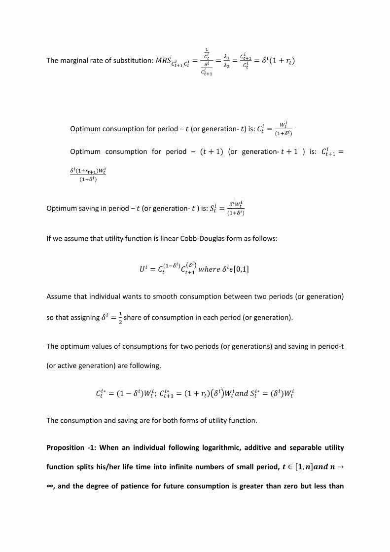
The marginal rate of substitution: �(���� ,� ��� =

*��3�

*�� �= ,

,4 = ��� ���� = ���1 + ���

Optimum consumption for period – � (or generation- �) is: ��� = 1�����+��

Optimum consumption for period – �� + 1� (or generation- � + 1 ) is: ����� =+����-�� �1��

���+��

Optimum saving in period – � (or generation- � ) is: ��� = +�1�����+��

If we assume that utility function is linear Cobb-Douglas form as follows:

"� = ����5+������%+�& 6ℎ8�8 ���[0,1]

Assume that individual wants to smooth consumption between two periods (or generation)

so that assigning �� = �9 share of consumption in each period (or generation).

The optimum values of consumptions for two periods (or generations) and saving in period-t

(or active generation) are following.

���∗ = �1 − ��� ��; �����∗ = �1 + ���%��& ����� ���∗ = ���� ��

The consumption and saving are for both forms of utility function.

Proposition -1: When an individual following logarithmic, additive and separable utility

function splits his/her life time into infinite numbers of small period, : ∈ [<, =]>=? = →∞, and the degree of patience for future consumption is greater than zero but less than

one [A < CD < 1] ,that means future consumption is less important than current

consumption, then the optimum consumption of current period becomes same as that of

the linear Cobb-Douglas utility function that logarithmic utility function becomes Cobb-

Douglas utility function (like the CES function transforms Cobb-Douglas function).3

Proof: If individual splits his/her life time into two-period then optimum consumption of

current period is- ���∗ = 1�����+�� .

If individual splits his/her life time into three-period then optimum consumption of current

period is- ���∗ = 1��[��+���+��4] .

If individual splits his/her life time into four-period then optimum consumption of current

period is- ���∗ = 1��[��+��%+�&4��+��E] .

If individual splits his/her life time into n-period then optimum consumption of current

period is- ���∗ = 1��[��+��%+�&4�%+�&E………��+��GH ] .

If � → ∞ ��� 0 < � < 1then the current period consumption is –

���∗ = ��[1 + �� + ����9 + ����I … … … + ����J5�] = �1 − ��� ��

This is nothing but the optimum consumption of current period if an individual follows linear

Cobb-Douglas from of utility function.

3Using the L’Hopital rule Constant Elasticity of Substitution( CES) utility function becomes Cobb-Douglas utility

function with limited value of zero. See derivation in appendix 1.3

Proposition-1.a: When an individual following logarithmic, additive and separable utility

function splits his/her life time into infinite numbers of small period, : ∈ [<, =]>=? = →∞, and the degree of patience for future consumption is one [CD = <] ,that means future

consumption gets equal important with current consumption, the optimum consumption

of current period is simply the income of current period,K:D divided by the numbers split,

=.

Proof: If individual splits his/her life time into two-period then optimum consumption of

current period is- ���∗ = 1��[��+�] .

If individual splits his/her life time into three-period then optimum consumption of current

period is- ���∗ = 1��[��+���+��4] .

If individual splits his/her life time into four-period then optimum consumption of current

period is- ���∗ = 1��[��+���+��4��+��E] .

If individual splits his/her life time into � − L8��.� ��� � → ∞, then optimum consumption

of current period is- ���∗ = 1��[��+���+��4��+��E……..�+���GH �] .

When the degree of patience for future consumption is one [�� = 1] then,

The optimum consumption of current period is- M:D∗ = K:D[<�=5<] = K:D

= .

2.a Family Behaviour with selfish (individualistic) attitude and different marginal utility of

money: Now assume that at any time-t there is a family in the economy consisting two

generations such as parent, P and adult-child, A. There is only one member of each

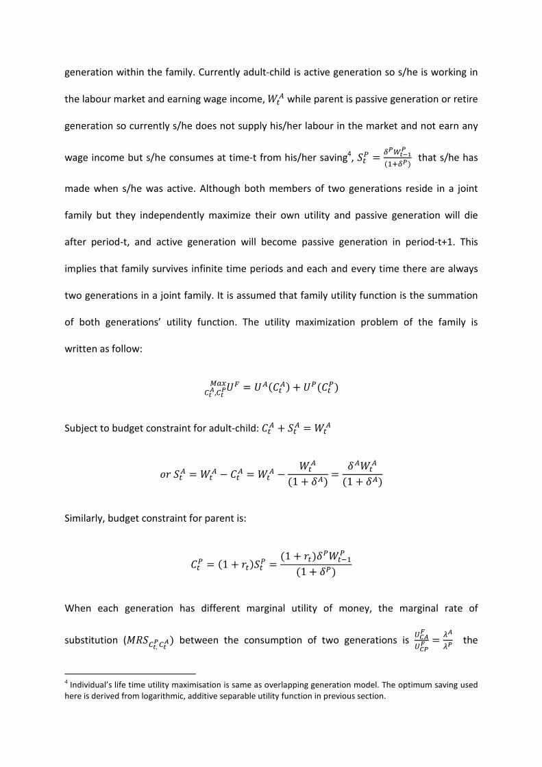
generation within the family. Currently adult-child is active generation so s/he is working in

the labour market and earning wage income, �N while parent is passive generation or retire

generation so currently s/he does not supply his/her labour in the market and not earn any

wage income but s/he consumes at time-t from his/her saving4, ��O = +P1�H P���+P� that s/he has

made when s/he was active. Although both members of two generations reside in a joint

family but they independently maximize their own utility and passive generation will die

after period-t, and active generation will become passive generation in period-t+1. This

implies that family survives infinite time periods and each and every time there are always

two generations in a joint family. It is assumed that family utility function is the summation

of both generations’ utility function. The utility maximization problem of the family is

written as follow:

"Q��R,��PSTU = "N���N� + "O���O�

Subject to budget constraint for adult-child: ��N + ��N = �N

.� ��N = �N − ��N = �N − �N�1 + �N� = �N �N�1 + �N�

Similarly, budget constraint for parent is:

��O = �1 + �����O = �1 + ����O �5�O�1 + �O�

When each generation has different marginal utility of money, the marginal rate of

substitution (�(���,P��R� between the consumption of two generations is )*RV)*PV = ,R

,P the

4 Individual’s life time utility maximisation is same as overlapping generation model. The optimum saving used

here is derived from logarithmic, additive separable utility function in previous section.

optimum condition which implies that the ratio of marginal utility of consumption between

two generations is equal to the ratio of marginal utility of money between two generations.

When marginal utility of money between two generations is equal then the optimum

condition says that marginal utility of consumption must be equal for both generations to

maximise family utility.

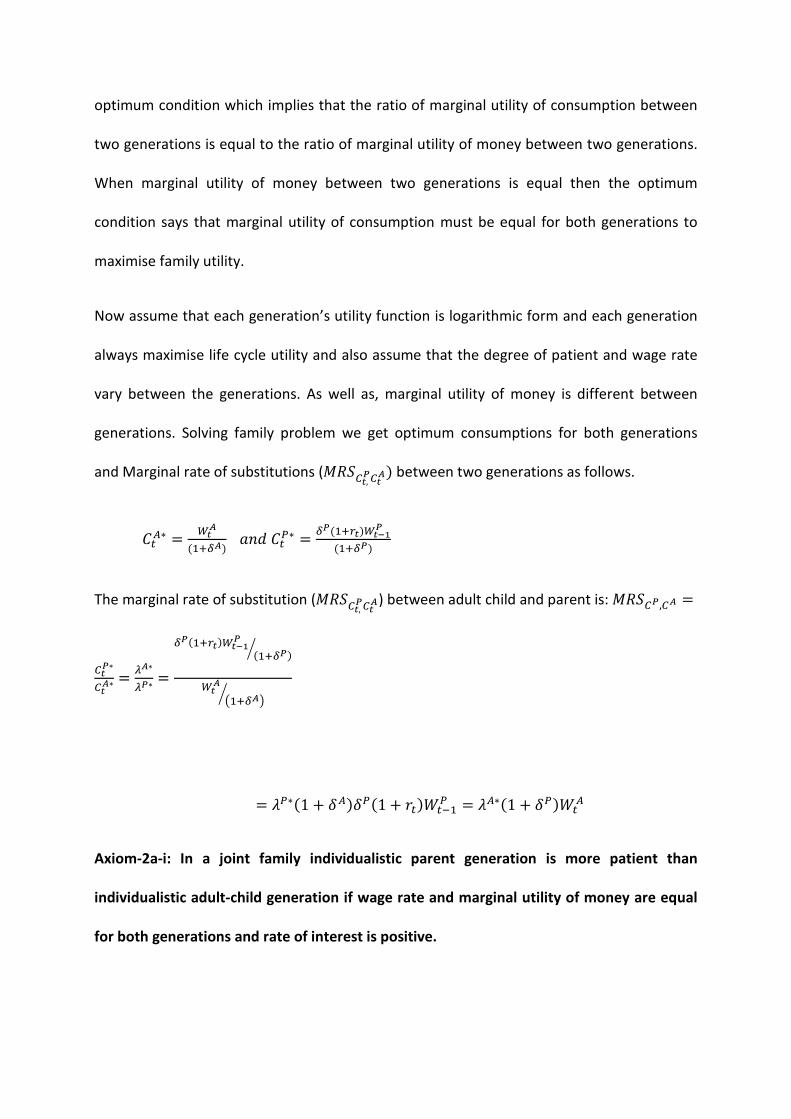
Now assume that each generation’s utility function is logarithmic form and each generation

always maximise life cycle utility and also assume that the degree of patient and wage rate

vary between the generations. As well as, marginal utility of money is different between

generations. Solving family problem we get optimum consumptions for both generations

and Marginal rate of substitutions (�(���,P��R� between two generations as follows.

��N∗ = 1�R���+R� ��� ��O∗ = +P���-��1�H P

���+P�

The marginal rate of substitution (�(���,P��R) between adult child and parent is: �(��P,�R =

��P∗��R∗ = ,R∗

,P∗ =+P���-��1�H P

���+P�W

1�R %��+R&W

= XO∗�1 + �N��O�1 + ��� �5�O = XN∗�1 + �O� �N

Axiom-2a-i: In a joint family individualistic parent generation is more patient than

individualistic adult-child generation if wage rate and marginal utility of money are equal

for both generations and rate of interest is positive.

Axiom-2a-ii: When degree of patience A < CY = CZ < 1 and marginal utility of money are

equal for both generations and rate of interest is positive then wage rate of adult

generation must be greater than that of the parent generation to maximise family utility.

2b. Family Behaviour with selfish (individualistic) attitude of each generation and same

marginal utility of money (Social Planner’s point of view): Now assume that each

generation belongs the same value of marginal utility of money that implies that there is a

social planner who likes to allocate resources for the consumption of adult child generation

and parent generation such a way that maximises a joint family’s utility. Therefore, the

planner combines the budget constraints of both generations into a family budget constraint

and maximizes family utility subject to family budget constraint.

The family budget constraint is: ��N + ��O = 1�R���+R� + �1 + ��� +P1�H P

���+P�

The family problem becomes as follows-

"Q��R,��P,,V,STU = "N���N� + "O���O� + XQ [ �N�1 + �N� + �1 + ����O �5�O�1 + �O� − ��N − ��O\

The marginal rate of substitution5 (�(���,P��R� between two generations is:

"�NQ"�OQ = 1 .� "�NQ = "�OQ

This implies that the marginal utility of consumption for each generation must be equal to

maximize family utility.

We also find that, 1�R%��+R& + ���-��+P1�H P

���+P� = ��N + ��O

5 Derivation is given in mathematical appendix-1.5.

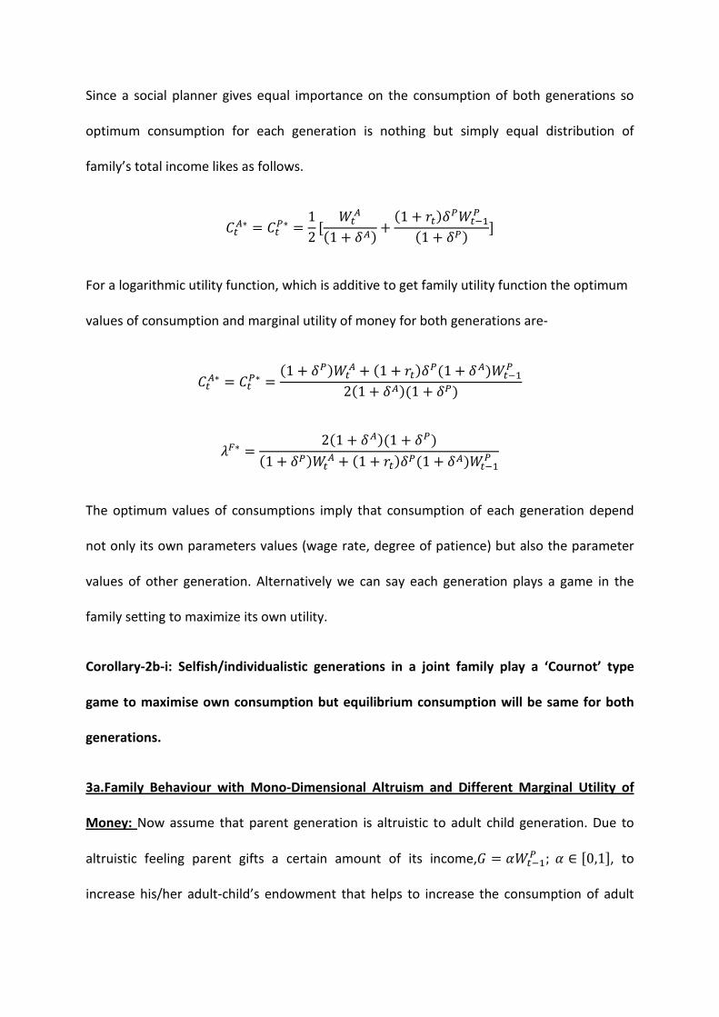
Since a social planner gives equal importance on the consumption of both generations so

optimum consumption for each generation is nothing but simply equal distribution of

family’s total income likes as follows.

��N∗ = ��O∗ = 12 [ �N�1 + �N� + �1 + ����O �5�O

�1 + �O� ]

For a logarithmic utility function, which is additive to get family utility function the optimum

values of consumption and marginal utility of money for both generations are-

��N∗ = ��O∗ = �1 + �O� �N + �1 + ����O�1 + �N� �5�O2�1 + �N��1 + �O�

XQ∗ = 2�1 + �N��1 + �O��1 + �O� �N + �1 + ����O�1 + �N� �5�O

The optimum values of consumptions imply that consumption of each generation depend

not only its own parameters values (wage rate, degree of patience) but also the parameter

values of other generation. Alternatively we can say each generation plays a game in the

family setting to maximize its own utility.

Corollary-2b-i: Selfish/individualistic generations in a joint family play a ‘Cournot’ type

game to maximise own consumption but equilibrium consumption will be same for both

generations.

3a.Family Behaviour with Mono-Dimensional Altruism and Different Marginal Utility of

Money: Now assume that parent generation is altruistic to adult child generation. Due to

altruistic feeling parent gifts a certain amount of its income,^ = _ �5�O ; _ ∈ [0,1], to

increase his/her adult-child’s endowment that helps to increase the consumption of adult

generation although the adult generation is selfish. In this situation family’s behaviour

becomes as follow-

The utility function of selfish adult child is: "N = "N���N�

The utility function of altruistic parent is: "O = "O���O� + ^"N���N�

"Q��R,��PSTU = �1 + ^�"N���N� + "O���O�

Subject to budget constraint for adult-child: ��N + ��N = �N + ^

.� ��N = �N + ^ − ��N = �N + ^ − �N�1 + �N� = �N �N�1 + �N� + ^

��N = �N�1 + �N�

Similarly, budget constraint for parent is:

��O = �1 + �����O − ^ = �1 + ����O �5�O�1 + �O� − ^

The marginal rate of substitution6 (�(���,P��R� between the consumption of two generations

is as follow. ���`�)*RV)*PV = ,R

,P .� )*RV)*PV = ,R

���`�,P

This is the optimum condition which implies that marginal utility of money to parent is lower

than that of his/her child, if their marginal utility of consumption held constant and vice

versa (the marginal utility of child consumption lower than that of parent so the total utility

of child will be higher than that of the parent.

6 Derivation is given in mathematical appendix-1.6

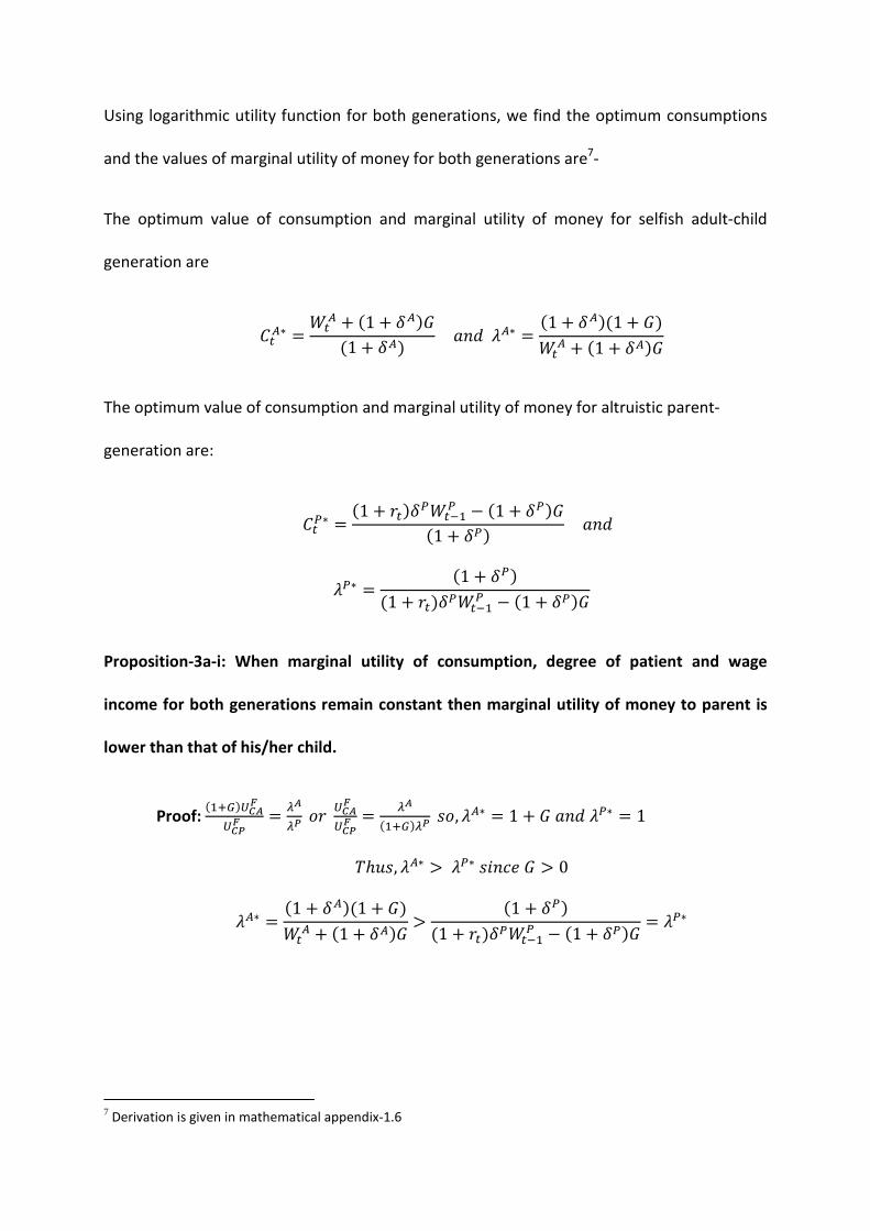
Using logarithmic utility function for both generations, we find the optimum consumptions

and the values of marginal utility of money for both generations are7-

The optimum value of consumption and marginal utility of money for selfish adult-child

generation are

��N∗ = �N + �1 + �N�^�1 + �N� ��� XN∗ = �1 + �N��1 + ^�

�N + �1 + �N�^

The optimum value of consumption and marginal utility of money for altruistic parent-

generation are:

��O∗ = �1 + ����O �5�O − �1 + �O�^�1 + �O� ���

XO∗ = �1 + �O��1 + ����O �5�O − �1 + �O�^

Proposition-3a-i: When marginal utility of consumption, degree of patient and wage

income for both generations remain constant then marginal utility of money to parent is

lower than that of his/her child.

Proof: ���`�)*RV

)*PV = ,R,P .� )*RV

)*PV = ,R���`�,P a., XN∗ = 1 + ^ ��� XO∗ = 1

bℎca, XN∗ > XO∗ a��e8 ^ > 0

XN∗ = �1 + �N��1 + ^� �N + �1 + �N�^ > �1 + �O�

�1 + ����O �5�O − �1 + �O�^ = XO∗

7 Derivation is given in mathematical appendix-1.6

Proposition-3a-ii: When marginal utility money, degree of patient and wage income for

both generations remains constant then total utility of child generation is higher than that

of parent generation.

Proof: )*RV)*PV = ,R

���`�,P a��e8XN∗ > XO∗ a��e8 ^ > 0 �ℎ8� "�NQ < "�OQ

Therefore, total utility of adult-child generation is higher than that of parent generation.

��N∗ = 1�R�%��+R&`���+R� > ���-��+P1�H P 5%��+P&`

���+P� = ��O∗

3b.Family Behaviour with Mono-Dimensional Altruism and same Marginal Utility of Money

(Social Planner’s Point of View): Assumed that marginal utility of money is same for both

generations that is family utility is maximized according to the social planner’s point of view.

Then the model becomes-

"Q��R,��PSTU = �1 + ^�"N���N� + "O���O�

Subject to, Family budget constraint: the budget constraint:

�N�1 + �N� + �1 + ����O �5�O�1 + �O� = ��N + ��O

The marginal rate of substitution (�(���,P��R� between the consumption of two generations

is - ���`�)*RV)*PV = 1 .� )*RV

)*PV = ����`�

This implies that the marginal utility of consumption for child is less than that of the parent.

It can be inferred that in this case total consumption of parent is lower than that of the

selfish parent but the opposite is the case for child’s consumption because marginal utility of

child consumption decreases means total utility increases.

Using the logarithmic utility function, the optimum values of consumption for both

generations are-

Optimum value of consumption for selfish adult-child is:

��N∗ = �1 + ^�[�1 + �O� �N + �1 + ����O�1 + �N� �5�O ]�2 + ^��1 + �N��1 + �O�

Optimum value of consumption for altruistic parent is:

��O∗ = [�1 + �O� �N + �1 + ����O�1 + �N� �5�O ]�2 + ^��1 + �N��1 + �O�

Proposition-3b-i: According to social planer’s point of view total consumption of an

altruistic parent generation is always lower than that of the selfish adult child generation.

Proof: �(���,P��R = )*RV)*PV = �

���`� < 1 a��e8 ^ > 0.

"�NQ < "�OQ �ℎ8�8f.�8, ��N∗ > ��O∗

From logarithmic utility function we get

��N∗ = �1 + ^�[�1 + �O� �N + �1 + ����O�1 + �N� �5�O ]�2 + ^��1 + �N��1 + �O�

> [�1 + �O� �N + �1 + ����O�1 + �N� �5�O ]�2 + ^��1 + �N��1 + �O� = ��O∗

Proposition-3b-ii: According to social planer’s point of view and mono-dimensional

altruistic family enjoys more total utility compared to selfish family.

Proof: The ratio of marginal utility of substitution between two generations of selfish family

to mono-dimensional altruistic family is-

�(���,P��R .f a8gf�aℎ f�h�gi�(���,P��R .f h.�. − ��h8�a�.��g �g��c�a��e f�h�gi =

11�1 + ^�

= �1 + ^� > 1.

This implies that, �(���,P��R of mono-dimensional altruistic family is lower than that of the

selfish family. Therefore, the total utility of mono-dimensional altruistic family is higher than

that of the selfish family. This proposition supports almost all mono-dimensional altruistic

literatures that altruistic behaviour improves family wellbeing. (Backer G.S, et.al 1979,

Altoniji et.al. 1997).

4a.Family Behaviour with Duo-Dimensional Altruisms and Different Marginal Utility of

Money: Now assume that both generations in a joint family are altruistic to each other but

their degree of altruism and marginal utility of money might be different. Further assume

that parent generation is altruistically spending ^ = _ �5�O ; _ ∈ [0,1] amount of his/her

income for its adult-child generation, on the other hand, adult-child generation is also

altruistically giving up j = k �N; k ∈ [0,1] amount of his/her income for looking after

his/her parent generation. The utility maximisation problem of this joint family becomes as

follow.

The utility function of child is: "�N = "N���N� + j"�O

The utility function of parent is: "�O = "O���O� + ^"�N

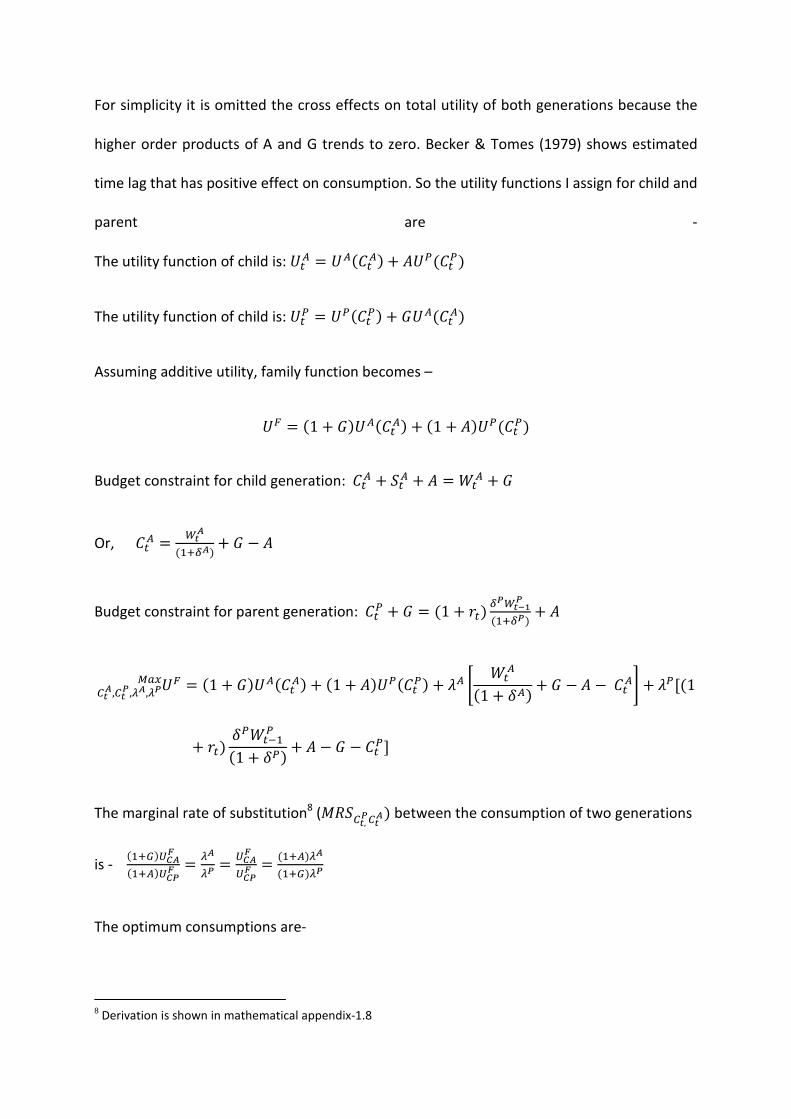
For simplicity it is omitted the cross effects on total utility of both generations because the

higher order products of A and G trends to zero. Becker & Tomes (1979) shows estimated

time lag that has positive effect on consumption. So the utility functions I assign for child and

parent are -

The utility function of child is: "�N = "N���N� + j"O���O�

The utility function of child is: "�O = "O���O� + ^"N���N�

Assuming additive utility, family function becomes –

"Q = �1 + ^�"N���N� + �1 + j�"O���O�

Budget constraint for child generation: ��N + ��N + j = �N + ^

Or, ��N = 1�R���+R� + ^ − j

Budget constraint for parent generation: ��O + ^ = �1 + ��� +P1�H P���+P� + j

"Q��R,��P,,R,,PSTU = �1 + ^�"N���N� + �1 + j�"O���O� + XN [ �N�1 + �N� + ^ − j − ��N\ + XO[�1

+ ��� �O �5�O�1 + �O� + j − ^ − ��O]

The marginal rate of substitution8 (�(���,P��R� between the consumption of two generations

is - ���`�)*RV���N�)*PV = ,R

,P = )*RV)*PV = ���N�,R

���`�,P

The optimum consumptions are-

8 Derivation is shown in mathematical appendix-1.8

An altruistic adult-child is-

��N∗ = �N�1 + �N� + ^ − j

An altruistic parent is-

��O∗ = �1 + ��� �O �5�O�1 + �O� + j − ^

Using logarithmic utility function the family utility maximisation problem is-

"Q��R,��P,,R,,PSTU = �1 + ^�g���N + �1 + j�g���O + XN [ �N�1 + �N� + ^ − j − ��N\ + XO[�1

+ ��� �O �5�O�1 + �O� + j − ^ − ��O]

The optimum consumption of an altruistic adult-child generation is-

��N∗ = XO�1 + ^��1 + ����O �5�OXN�1 + j��1 + �O� + XO�1 + ^��j − ^�

XN�1 + j�

Optimum marginal utility of money for adult-child is

XN∗ = �1 + ^��1 + �N� �N + �1 + �N��^ − j�

The optimum consumption of an altruistic parent generation is-

��O∗ = XN�1 + j� �NXO�1 + ^��1 + �N� + XN�1 + j��^ − j�XO�1 + ^�

Optimum marginal utility of money for parent is

XO∗ = �1 + j��1 + �O��1 + ����O �5�O + �1 + �O��j − ^�

Proposition-4a-i: If the degrees of patient, amount of transfer and wage income of both

generations are equal then values of marginal utility of money for both generations must

be equal.

Proof: �(���,P��R = ���`�)*RV���N�)*PV = ,R

,P = )*RV)*PV = ���N�,R

���`�,P �f j = ^ ��� "�NQ = "�OQ

ThenXN = XO. Using logarithmic function,

XN∗ = �1 + ^��1 + �N� �N + �1 + �N��^ − j� = �1 + j��1 + �O�

�1 + ����O �5�O + �1 + �O��j − ^� = XO∗

Proposition-4a-ii: If values of marginal utility of money and the altruistic transfers are

equal then total utility of consumption for both generations is same.

Proof: �(���,P��R = ���`�)*RV���N�)*PV = ,R

,P = )*RV)*PV = ���N�,R

���`�,P = 1�f XN = XO��� j = ^

Then, "�NQ = "�OQ the marginal utility of consumption equal means total utility of both

generations must be equal. Using logarithmic utility function,

��N∗ = XO�1 + ^��1 + ����O �5�OXN�1 + j��1 + �O� + XO�1 + ^��j − ^�

XN�1 + j�= XN�1 + j� �NXO�1 + ^��1 + �N� + XN�1 + j��^ − j�

XO�1 + ^� = ��O∗

Proposition -4a-iii: When marginal utility of money and wage income for both generations

is same then altruistic family behaviour would be same as individualistic family behaviour

if mutual transfers from both generations are identical that means A=G.

Proof: �f XN = XO��� j = ^

The ratio of ��(���,P��R� between the consumption of two generations of

selfish/individualistic model to duo-dimensional altruistic model is-���`����N�=1. So there is no

difference between duo-altruistic model and individualistic family utility maximisation.

Altruistic adult child consumption is -��N∗ = ,P���`����-��+P1�H P,R���N����+P� + ,P���`��N5`�

,R���N�

��N∗ = ���-��+P1�H P���+P� = 1�R

���+R� = ���∗= Individualistic adult child consumption.

Altruistic parent consumption is –��O∗ = ,R���N�1�R,P���`�%��+R& + ,R���N��`5N�

,P���`�

��O∗ = ,R���N�1�R,P���`�%��+R& = ���-��+P1�H P

���+P� = ��5��∗ =Individualistic parent consumption.

4b.Family Behaviour with Duo-Dimensional Altruisms having same Marginal Utility of

Money (Social Planner Point of View):

Now assume that both generations are altruistic to each other and their degree of altruism

might be different but marginal utility of money is same. The family problem becomes now

as following.

"Q��R,��P,,V,STU = �1 + ^�"N���N� + �1 + j�"O���O�

+ XQ [ �N�1 + �N� + �1 + ��� �O �5�O�1 + �O� − ��N − ��O\

The marginal rate of substitution9 (�(���,P��R� between the consumption of two generations

is - ���`�)*RV���N�)*PV = 1 = )*RV

)*PV = ���N����`�. This implies that the marginal rate of substitution depends

on the value of altruistic transfers of both generations A and G. When A>G, marginal utility

of child’s consumption is higher than that of the parent’s. So parent’s total utility is higher

than that of child’s and the opposite would be true if G>A.

If social planner gives equal importance on the consumption of both generation then

optimum consumption is half of total family income, which has no difference from

individualistic case.

��N∗ = ��O∗ = 12 [ �N�1 + �N� + �O �5�O

�1 + �O�]

Using logarithmic utility function we get optimum consumption of both generations as

follows.

The optimal consumption of altruistic adult generation is as follows:

��N∗ = �1 + ^��1 + �O� �N + �1 + ����O�1 + �N� �5�O�2 + ^ + j��1 + �N��1 + �O�

The optimal consumption of altruistic old (parent) generation is as follows:

��O∗ = �1 + j��1 + �O� �N + �1 + ����O�1 + �N� �5�O�2 + ^ + j��1 + �N��1 + �O�

We also get the marginal utility of money for both generations is as follows:

XQ∗ = �2 + ^ + j��1 + �N��1 + �O��1 + �O� �N + �1 + ����O�1 + �N� �5�O

9 Derivation is given mathematical appendix-1.9

Proposition-4b-i: When altruistic transfer of adult-child towards parent is bigger than that

of parent towards adult-child, Y > ^, marginal utility of child’s consumption is higher than

that of the parent’s. So parent’s total utility is higher than that of child’s and the opposite

would be true if the condition revised, that is G>A.

Proof: �(���,P��R = ���`�)*RV���N�)*PV = 1 = )*RV

)*PV = ���N����`�

�f j > ^ �ℎ8�, "�NQ > "�OQ a. �.��g c��g��i .f ��cg� − eℎ�g� < b.��g c��g��i .f L��8��

The ratio of optimal consumption is:��R∗��P∗ =

� �l�m �3Pno�R�� �p��3P� �3R�o�H P�4�l�R�% �3R&� �3P�

� �R�% �3P&o�R�� �p��3P� �3R�o�H P�4�l�R�% �3R&� �3P�

= ��`��N

�f j > ^ �ℎ8�, ��N∗ < ��O∗ and, �f j < ^ �ℎ8�, ��N∗ > ��O∗

Why is joint family structure breaking in developed and developing countries?

In developing countries:

It is usual that child altruistic transfer to parent (A) must not be equal to the parent’s

altruistic transfer to child (G). Becker & Tomes (1979) show that parent’s transfer to child

increases child’s productivity which leads to increase child wage income along with

economic growth enhances child’s wage income compare to his/her parent. So child’s

transfer to his/her parent (A) might be bigger than that of the parent’s (G). Then the

�(���,P��R is greater than one and total consumption of child is less than that of his/her

parent. Parent is better off than child. It is also assumed that parent’s transfer to child (G)

and Child’s transfer to parent (A) are respectively _ ��� k [�0,1]share of corresponding

generation’s wage income. If a child wants to increase his/her total consumption in the

family s/he needs to reduce the value of degree of altruismk, which leads the child to

behave selfishly and motivate to stay separately not in a family. That implies that economic

growth of developing countries and altruistic transfers from parent leads child-generation to

break co-residing family structure and to construct nuclear family live.

In developed Countries:

If parent transfer to child (G) is bigger than child’s transfer (A) due to high value of his/her

degree of altruism _, and marginal utility of money remains same for both generations then

total consumption of parent would be lower than that of his/her child-generation. So parent-

generation wants to reduce the value of _ , to increase his/her total consumption in the

family. This leads to parent-generation to break family structure and reside selfishly in a

nuclear family. In developed countries where social security system is very much advanced

and reliable for both child-generation and parent-generation then both generation want to

reduce the values of their corresponding degree of altruistic feeling _ and k, to increase the

share of their total consumption in a joint family setting. The continuous reduction of the

value of altruistic emotion leads each generation to behave selfishly and construct nuclear

family structure.

Empirical Evidence:

Model selection: It is usual to convert theoretical model into a suitable empirical model

which is accommodated with relevant and available data set. I theoretically develop the

conclusion that joint family structure of a society is changing mainly because of wage rate

differential and difference of social and cultural emotions i.e. altruistic emotions between

generations. According to my definition of joint family, an elderly generation must reside

with a younger generation. I, therefore, choose the percentage of elderly men or women

living with at least a child or grandchild as a proxy of measuring the number of joint family in

a society because it captures at least two generations co-residing in a family. According to

my theory, increasing a generation’s income leads to construct nuclear family by breaking

the joint family to maximise that generation’s total utility. I, therefore, assume that per

capita GDP of a country might be a good proxy variable10 to empirically evaluate a

generation’s income and the relationship between these two variables might be negative i.e.

when per capita GDP of a generation increases then that generation wants to live

independently and less likely to stay with elderly people. It is natural to assume that each

and every generation by born grasps some degree of altruistic emotion toward other

generation and needs co-operation among themselves in several stages in a life cycle, so

each generation likes to stay in a joint family structure. This implies annual population

growth rate leads to increase the probability of new generation stays in a joint family. But

when the population growth is due to increase in the stock of migrated people then

depending on other socio-economic circumstances these people may or may not stay in a

joint family structure. So it does not always give us a clear picture of living arrangement of a

society11. Thus the stock of migrated people either positively or negatively affects the living

arrangement of a society. It is usual that development of urban amenities and stresses will

lead a generation to construct a nuclear family because of high residential cost,

unemployment rate, severe competition in living style etc. (Manacorda and Moretti, 2002).

Even more than the economic and demographic points of view, living arrangement mainly

depend on social norms, values, religions, traditions, rules and obligations etc. Each region in

10 Some literatures say changing growth rate might be a good proxy of per capita GDP in mostly for developing

countries but I do believe that later one is more stable than the former and less affected by short run shock. 11 Some literatures include the number of migrated people in co-residence behaviour analysis such as Cheolsung

Park (2001).

the world such as Asia, Europe or Africa has some distinctive sorts of social characteristics

and these characteristics must directly influence living style of that region. Above all, the

state of development of a country must influence co-residence behaviour of the people. It is

assumed that in a developed society joint family structure is less important than that of a

developing society because ‘market insurance is used instead of kin insurance, market

schools instead of family schools, and examinations and contracts instead of family

certification’ (Becker, 1981) and public social security transfer benefits instead of familial

social security transfers. One, therefore, may conclude that the more developed a country

the less joint family structure is existed in the society.

To make the empirical model easily estimable I, therefore, choose three economic variables,

two demographic variables and a regional dummy variable discussed in earlier paragraph.

Three economic variables are: (i) per capita GDP, (ii) nature of development of a country

which is a dummy variable such as developed country, newly developed countries and least

developed countries, and (iii) proportion of total population lives in urban region of a

country; two demographic variables are: (i) population growth rate and (ii) percentage of

stock of migrated people of a country; and the regional dummy variable includes to cover

common effect of social characteristics. All these variables are included as independent

variables in a linear additive functional form of multivariate regression model and the

dependent variable is percentage of elderly people living with a child or grandchild. I follow

the step regression system by starting with one numerical variable and two dummy variables

as explanatory variables and step by step include other three numerical variables with the

first one. This method of estimation helps me to specify the effect of each explanatory

numerical variable in the estimation process and to diagnose statistical significance of the

variable in the linear regression process – which is a common way of specifying an empirical

model. I estimate the linear functional form of following equations both by

heteroscadasticity adjusted ‘OLS’ estimation technique and simple OLS technique to specify

proper empirical model that supports my theoretical model. Each functional form is

estimated twice – one for elderly men and another for elderly women.

qrq��� = q^sq� + jt(u� + j�uj� + r"(v� + wbj�� + wsrx� + ysrx� + "� − − − 1

qrq� � = q^sq� + jt(u� + j�uj� + r"(v� + wbj�� + wsrx� + ysrx� + "� − − − 2

qrq��� = q^sq� + q��q� + jt(u� + j�uj� + r"(v� + wbj�� + wsrx� + ysrx� + "�− − − 3

qrq� � = q^sq� + q��q� + jt(u� + j�uj� + r"(v� + wbj�� + wsrx� + ysrx� + "�− − − 4

qrq��� = q^sq� + jq^(� + jt(u� + j�uj� + r"(v� + wbj�� + wsrx� + ysrx� + "�− − − 5

qrq� � = q^sq� + jq^(� + jt(u� + j�uj� + r"(v� + wbj�� + wsrx� + ysrx� + "�− − − 6

qrq��� = q^sq� + q"qy� + jt(u� + j�uj� + r"(v� + wbj�� + wsrx� + ysrx� + "�− − − 7

qrq� � = q^sq� + q"qy� + jt(u� + j�uj� + r"(v� + wbj�� + wsrx� + ysrx� + "�− − − 8

qrq��� = q^sq� + q��q� + jq^(� + jt(u� + j�uj� + r"(v� + wbj�� + wsrx�+ ysrx� + "� − − − 9

qrq� � = q^sq� + q��q� + jq^(� + jt(u� + j�uj� + r"(v� + wbj�� + wsrx�+ ysrx� + "� − − − 10

qrq��� = q^sq� + q��q� + q"qy� + jt(u� + j�uj� + r"(v� + wbj�� + wsrx�+ ysrx� + "� − − − 11

qrq� � = q^sq� + q��q� + q"qy� + jt(u� + j�uj� + r"(v� + wbj�� + wsrx�+ ysrx� + "� − − − 12

qrq��� = q^sq� + q"qy� + jq^(� + jt(u� + j�uj� + r"(v� + wbj�� + wsrx�+ ysrx� + "� − − − 13

qrq� � = q^sq� + q"qy� + jq^(� + jt(u� + j�uj� + r"(v� + wbj�� + wsrx�+ ysrx� + "� − − − 14

qrq��� = q^sq� + q��q� + jq^(� + q"qy� + jt(u� + j�uj� + r"(v� + wbj��+ wsrx� + ysrx� + "� − − − 15

qrq� � = q^sq� + q��q� + jq^(� + q"qy� + jt(u� + j�uj� + r"(v� + wbj��+ wsrx� + ysrx� + "� − − − 16

Where,

qrq���= The percentage of elderly men (60 years and above) living with at least a child or a

grandchild of the country-i.

qrq� �= The percentage of elderly women (60 years and above) living with at least a child

or a grandchild of the country-i.

q^sq�= Per capita GDP of the country-i, which might be inversely related with the

dependent variable.

q��q�= Percentage of stock of migrated people in the country-i, which may or may not be

positively related with dependent variable.

jq^(�= Annual population growth rate of the country-i, which might be directly related

with dependent variable.

q"qy�= Percentage of urban population of the country-i, which is expected to be negatively

related with dependent variable.

jt(u�= It is a regional dummy variable included in the regression model to cover social

norms, values, rules, religions, etc of that region. Here, it takes value=1 if the country is

situated in African region otherwise it takes value = 0.

j�uj�= It is a regional dummy, it takes value =1 if the country is situated in Asian region

otherwise it takes value = 0.

r"(v�= It is a regional dummy, it takes value=1 if the country is located in European region

otherwise it takes value = 0.

wbj��= It is a regional dummy, it takes value=1 if the country is situated in Latin America or

the Caribbean otherwise it takes value = 0.

wsrx�= It is a dummy variable covering least developed status of a country compared to the

others. It takes value =1 value if the per capita GDP of a country-i is lower than $5000 in the

PPP measurement of 1995, otherwise it takes value =0.

ysrx�= It is also dummy variable indicating newly developed status of a country, It takes =1

value if the per capita GDP of the country-i is lower than $12000 but higher than $5000 in

the PPP measurement of 1995 otherwise =0.

"�= Disturbance term of a country-i’s observation which is assumed to be normally,

independently distributed with zero means and constant variance.

Sources of Data: The percentage of the elderly people living with a child or grandchild is

collected from ‘the Executive Summary - the Annex I:A, iv.1:’ of the United Nations

Population Divisions, Department of Economic and Social Affairs in a title ‘Living

Arrangements of Older Persons Around the World’ which covers 75 countries of which 20

countries are from African region, 20 countries are from Asian region, 18 and 16 countries

are from European and Latin America and the Caribbean respectively and the United States

of America. All most all observations of dependent variable are from period 1998, 1999 or

2000 but there are some countries’ information which has been reported between 1991 and

1998 due to unavailability of 1999 or 2000 information12. Data on four independent

numerical variables are collected from the ‘Country Profile’ of the United Nations Population

Division for the year 2000.The percentage of stock of migrated people is calculated by using

this formula.

12 I think most of countries use 10 years time difference between two population censuses. So It is justifiable to

use one census information until the next census information would be available.

q8�e8����8 .f a�.e� .f h�����8� L8.Lg8= b.��g ��.e� .f ���8�����.��g h�����8� L8.Lg8

b.��g L.Lcg���.� �100

Then I pool data of dependent variable with that of independent variables. I think it is

reasonable to call this data set as cross section polled data of cross country not as cross

section panel data of cross country because all observations of all independent variables of

each country are basically in the year 2000 point except the dependent variable. There is no

observation on another point of time.

Results and Discussions:

The above 16 estimated regression equations indicate that dependent variable and

independent variables are nearly perfectly causally related because each of these estimated

equations has both robust and adjusted (9 −value more than 0.80. As well as all variables

have expected sign and majority of them are significant at below 5% error level. In the

following table I just have reported two estimated equations – one is for elderly men living

with a child or grandchild and another is for elderly women by including all independent

numerical variables and dummy variables using ‘Robust OLS estimation’ technique in Table-2

and Table-3 of appendix all estimated results have provided. From these reported estimated

equations one can easily say that elderly people is less likely to co-reside with a child or

grandchild in a country having high per capita GDP (PGDP) and the argument is statistically

significant below 5% error level in case of elderly women but the elderly men’s case has

expected sign although not statistically significant at 5% error level. The estimated co-

efficient of PGDP variable in case elderly women says that one percent increase in per capita

GDP of a country will decrease 0.09% probability of elderly women’s co-residing status in a

joint family. The percentage of stock of migrated population (PSMP) is statistically

insignificant in both reported estimated equations but the positive sign in both cases implies

that migrated people are like to co-reside in a joint family.13 The annual population growth

rate (APGR) variable is significant below 10% error level in both reported equations and has

expected positive sign. The estimated value of co-efficient for this variable tell us that 1%

increase in population growth rate will rise 3.40% and 1.89% of co-residing possibility of

elderly men and women respectively. The percentage of population living in urban area

(PUPN) is statistically significant at 10% error level in case elderly men but in significant for

women. In both equations the PUPN variable has expected negative sign which implies that

urban people are more likely to live in a nuclear family setting rather than rural people in

every country. The estimated co-efficient of the variable PUPN for men indicates that the

0.14% probability decreases of elderly men co-residence attitude due to 1% percent increase

in urban population of a country. All the regional dummy variables (AFRI, ASIA, EURO and

LTAM) are highly significant and positive sign expect the European region which has negative

sign and insignificant co-efficient value. The positive sign of these regional dummy indicates

that sociological characteristics are very much influential to a generation to determine its

residence decision. The highest positive value of estimated coefficient among these four

regional dummies is 45.28 and 37.90 which is obtained from Asian region from the

estimated equation of elderly men and women respectively. The highest score indicates

both that Asian people are more likely to stay in join family and that they are more

influenced by social characteristics compared to other regions. The negative sign of regional

dummy for Europe although not statistically significant indicates that European sociological

characteristics support nuclear family attitude. Two dummy variables (LDEV and NDEV)

13 We know omission of a relevant explanatory variable is more harmful than inclusion of an irrelevant variable.

Since the sign of estimated coefficient explain some behaviour I include this variable in reported equation.

indicating development status are statistically insignificant although both belong expected

negative sign. The negative sign of these dummy variables imply that economic development

of a country motivates a generation to construct nuclear family leaving from joint family. In

any regression equation having dummy explanatory variable constant co-efficient is very

important causal relation with dependent variable if estimation process is not forcefully

excluded constant term. This term covers estimated value of base dummy which, in my

estimated equations, is the USA. The co-efficient of constant term is highly significant in all

cases and positive sign. The overall consequence of regional dummy, development dummy

and constant term gives positive estimated co-efficient for all estimated equations both

elderly men and women cases. These might have several interpretations such as (i)

sociological characteristics are more influential than economic development indicator of

country; and (ii) the probability of overall co-residence decision is improve due to a unit

change of these dummy variables. These empirical findings support the conclusion that co-

residence decision of a generation depends on both economic and social variables.

Reported Regression Results

Estima

ted

Dept.

Variab

le

Const.

Co-

efft.

Co-efft.

of PGDP

Co-

efft.

of

PSM

P

Co-

efft.

of

APG

R

Co-

efft.

of

PUPN

Co-

efft.

of

AFRI

Co-

efft.

of

ASIA

Co-

efft.

of

EUR

O

Co-

efft.

of

LTAM

Co-

efft.

of

LDEV

Co-

efft.

of

NDE

V

(9

Valu

e

qr�q�� 38.30�12.70�∗ −0.00046�0.00044� 0.048 �0.179

3.40∗∗�1.89� −0.14�0.08�

∗ 37.24�8.90�∗∗ 45.28�8.09�

∗∗ 5.47�5.93� 35.61�8.69�∗∗ −3.23�8.46�

∗ −2.85�6.94� 0.88

(std.

err)

qr�q � 53.21�11.90�∗ −0.0009�0.00042� 0.057 �0.159

1.89∗∗�1.12� −0.12

(0.08

)

29.55�8.78�∗∗ 37.90�7.79�

∗∗ −2.59�5.72� 30.02�8.24�∗∗ −11.76�8.18� −5.70�6.77� 0.88

(std.

err)

Conclusions: Changing family structure all over the world is not occurring due to a uniform

reason and the nature and type of change are not also unique in a sense that currently,

family structure in developed countries moves from nuclear family to living together system

(between heterogeneous sex or homogeneous sex) and in developing countries it turns from

traditional joint family to nuclear family. There must be several distinct reasons of changing

family structure in these two worlds. In this paper, I have theoretically as well as empirically

found out that changing degree of altruistic emotion along with wage rate differential

among generations, which leads to change in family structure. The most important thing

that I have proved in this paper is that in an infinite time horizon over lapping generation

model, the optimum current period consumption getting from a logarithmic utility function

is equal to that of the Cobb-Douglas utility function when degree of patience is less than

unity. Another important feature of this paper is that the maximum utility of a duo-

dimensional altruistic family consisting two generations would be equal to

individualistic/selfish exchange family when the amount of altruistic transfer between

generations is equal although mono-dimensional altruistic family produces more total utility

than selfish exchange family. This conclusion leads me to say that any social planner should

follow mono-dimensional altruistic familial transfer no matter what the direction of transfer

may be, (working generation to retire generation for developed countries and retire

generation to working generation for developing countries) to enhance social well-being.

The empirical results suggest that per capita GDP, annual population growth rate,

percentage of urban population and the most important sociological characteristics are

statistically significant determinants of co-residence decision of a country which supports my

theoretical propositions.

References:

Altig D, SJ Davis (1992) ‘The Timing of Intergenerational Transfers, Tax Policy, and Aggregate

Savings’ American Economic Review, 82(5):1199-1220.

Altonji JG, F Hayashi, and LJ Kotlikoff (1997) ‘Parental Altruism and Inter Vivos Transfers:

Theory and Evidence’ Journal of Political Economy, 105(6):1121-1166.

Arrondel L, A Masson (2001) ‘Family Transfers Involving Three Generations’ The

Scandinavian Journal of Economics, 103(3) Intergenerational Transfers, Taxes and the

Distribution of Wealth: 415-443.

Arrow KJ (1971) ‘A Utilitarian Approach to the Concept of Equality in Public Expenditures’

The Quarterly Journal of Economics, 85(3): 409-415.

Arthur BW, M Geoffrey (1977) ‘Optimal Time Path with Age-Dependence: A Theory of

Population Policy’ The Review of Economic Studies, 44(1): 111-123.

Arthur BW, M Geoffrey (19780 ‘Samuelson, Population and Intergenerational Transfer’

International Economic Review, 19(1): 241-246.

Bangladesh Bureau of Statistics (2007). Population Census-2001, National Series, Vol. -1,

Analytical Report: 153.

Barro RJ (1978) The Impact of Social Security on Private saving: Evidence from the U.S. Time

Series. Washington D.C: American Enterprise Institute for Public Policy Research.

Barro RJ (1974) ‘Are Government Bonds Net Worth?’ Journal of Political Economy, 82(6):

1095-1117.

Bernheim BD, A Shleifer and LH. Summers (1985) ‘The Strategic Bequest Motive’ Journal of

Political Economy, 93(6): 1045-1076.

Becker GS, LH Gregg (1973) ‘On the Interaction between the Quantity and Quality of

Children’ Journal of Political Economy, 81(2-II): s279-s288.

Becker GS (1974) ‘A Theory of Social Interactions’ Journal of Political Economy, 82(6): 1063-

1093.

Becker GS, N Tomes (1979) ‘An Equilibrium Theory of the Distribution of Income and

Intergenerational Mobility’ Journal of Political Economy, Vol. 87, No. 6, (Dec., 1979), pp.

1153-1189.

Becker GS (1981) A Treatise of the Family, Harvard University Press, p.243.

Becker GS, RJ Barro (1988) ‘A Reformulation of the Economic Theory of Fertility’ The

Quarterly Journal of Economics, 103(1): 1-25.

Bengston, Vern. 2001. "Beyond the nuclear family: The increasing importance of multi-

generational bonds." Journal of Marriage & the Family 63:1-19.

Bryson, Ken and Lynne M. Casper. 1999. "Coresident grandparents and grandchildren.

Current population reports, special studies." U.S. Department of Commerce, Economics and

Statistics Administration, U.S. Census Bureau., Washington D.C.

Blanchard Olivier J. (1985) ‘Debt, Deficit, and Finite Horizons’. The Journal of Political

Economy, 93(2, April): 223-247.

Boswell J. (1959) Boswell for the Defence, 1769-1774 ed. New York, McGraw-Hill.

Casper, Lynne M. and Kenneth R. Bryson. 1998. "Co-resident grandparents and their

grandchildren: Grandparent maintained families." in Population Division Working Paper.

Chiappori, P-A. (1992). ‘Collective Labour Supply and Welfare’, Journal of Political Economy,

100: 437-67.

Cox D (1987) ‘Motives for Private Income Transfers’ The Journal of Political Economy, 95(3):

508-546.

Diamond PA (1965) ‘National Debt in a Neoclassical Growth Model’ The American Economic

Review, 55(5 Part-1): 1126-1150.

Dutta J, and M Philippe (1998) ‘The Distribution of Wealth with Imperfect Altruism’ journal

of economic theory, 82: 379-404.

Ermisch J and Pronzato C (2008). ‘Intra-Household Allocation of Resources: Inferences from

Non-resident Fathers’ Child Support Payments’ The Economic Journal 118(527): 347-363.

Feldstein M (1974) ‘Social Security, Induced Retirement, and Aggregate Capital

Accumulation.’ The Journal of Political Economy, 82(5): 905-926.

Frankenberg E, L Lillard and RJ Willis (2002) ‘Patterns of Intergenerational Transfers in

Southeast Asia’ Journal of Marriage and the Family, 64(3): 627-641.

Friedman DD (1987) ‘Does Altruism produce Efficient Outcomes? Marshall vs. Kaldor’- A

memo.

Friedman, M. (1957). ‘A Theory of Consumption Function’ National Bureau of Economic

Research, Princeton University Press.

Geanakoplos John D. and Heraklis M. Polemarchakis (1991) Handbook of Mathematical

Economics, Volume-iv, Elsevier Science Publishers: 1900-1960.

Hamoudi A, D Thomas (2006) ‘Do You Care? Altruism and Inter-Generational Exchanges in

Mexico’ On-Line Working Paper Series, California Center for Population Research, University

of California-Los Angeles, CCPR-008-06.

Herskovits Melville J. (1965) Economic Anthropology New York: W. W. Norton.

Ita F, O Stark (2001) ‘Dynasties and Destiny: On the Roles of Altruism and Impatience in the

Evolution of Consumption and Bequests’ Economica, New Series, 68(272): 505-518

Lee RD (1980) ‘Age Structure Intergenerational Transfers and Economic Growth: An

Overview’ Revue economique 6(Nov): 1129-1156.

Light A, K McGarry (2004) ‘Why Parents Play Favorites: Explanations for Unequal Bequests’

The American Economic Review, 94(5): 1669-1681.

Lillard LA and Willis RJ (1997) ‘Motives for intergenerational transfers: Evidence from

Malaysia’ Demography 34, 115-134.

Manacorda M and Moretti E (2002). ‘Intergenerational Transfers and Household Structure

Why do Most Italian Youths Live With Their Parents?’ California Center for Population

Research-011-03.

Mason, Karen Oppenheim (1992). ‘Family Change and Support of the Elderly in Asia:

What Do We Know?’, Asia-Pacific Population Journal 7(3): 13-32.

Pal S. (2007) ‘Effects of Intergenerational Transfers on Elderly Coresidence with Adult

Children: Evidence from Rural India, IZA discussion paper no 2847.

Park C. (2001) ‘Is Extended Family in Low-Income Countries Altruistically Linked? Evidences

from Bangladesh’, Department of Economics, National University of Singapore.

Posner RA (1980) ‘A theory of Primitive Society, with Special Reference to Law’ Journal of

Law and Economics 23(1): 1-53.

Rangel, M.A. (2006). ‘Alimony rights and intrahousehold allocation of resources: evidence

from Brazil’. Economics Letters, 13: 207-11.

Sakudo M. (2007) ‘Strategic Interactions between Parents and Daughters: Co-residence,

Marriage and Intergenerational Transfers in Japan’ Job market paper.

Samuelson PA (1958) ‘An Exact Consumption-Loan Model of Interest with or without the

Social Contrivance of Money’ The Journal of Political Economy, LXVI(6): 467-482.

Simmons, T. and J. Dye. 2003. "Grandparents living with grandchildren." U.S. Department of

Commerce, Economics and Statistics Administration, U.S. Census Bureau., Washington, D.C.

Sloan FA, HH. Zhang and J Wang (2002) ‘Upstream Intergenerational Transfers’ Southern

Economic Journal, 69(2): 363-380.

Solomon, J. and J. Marx. 1995. ""To grandmother's house we go": Health and school

adjustment of children raised solely by grandparents." The Gerontologist 35:386-394.

United Nations (2005). Living Arrangements of Older Persons Around the World

(http://www.un.org/esa/population/publications/livingarrangement/report.htm),

downloaded 15 September2008.

Weiss, Y. And Willis, R.J. (1985). ‘Children as collective goods and divorce settlements’

Journal of Labor Economics, 3:268-92

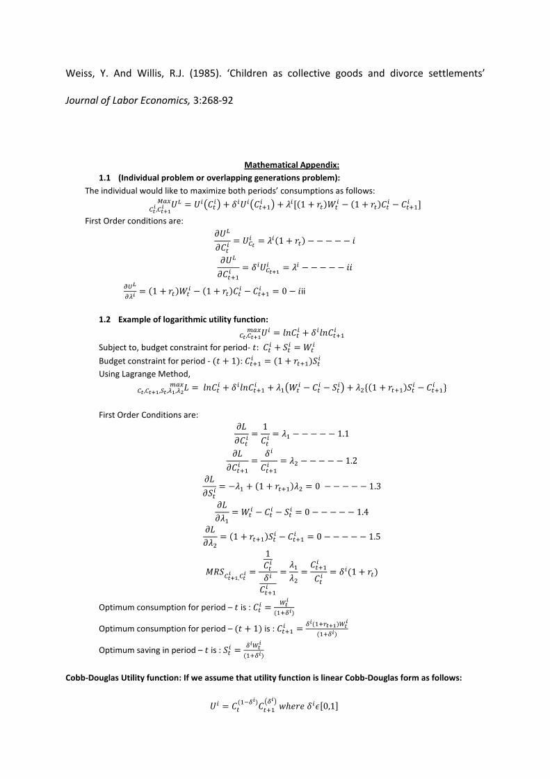
Mathematical Appendix:

1.1 (Individual problem or overlapping generations problem):

The individual would like to maximize both periods’ consumptions as follows:

"#���,��� �STU = "�%���& + ��"�%����� & + X�[�1 + ��� �� − �1 + ������ − ����� ]

First Order conditions are:

�"#����

= "��� = X��1 + ��� − − − − − �

�"#������ = ��"��� � = X� − − − − − ��

�)��,� = �1 + ��� �� − �1 + ������ − ����� = 0 − �ii

1.2 Example of logarithmic utility function:

"� = g���� + ��g��������,��� �TU

Subject to, budget constraint for period- �: ��� + ��� = �� Budget constraint for period - �� + 1�: ����� = �1 + �������� Using Lagrange Method,

w��,��� ,!�,, ,,4�TU = g���� + ��g������ + X�% �� − ��� − ���& + X9{�1 + �������� − ����� }

First Order Conditions are:

�w����

= 1���

= X� − − − − − 1.1

�w������ = ��

����� = X9 − − − − − 1.2

�w����

= −X� + �1 + �����X9 = 0 − − − − − 1.3

�w�X� = �� − ��� − ��� = 0 − − − − − 1.4

�w�X9 = �1 + �������� − ����� = 0 − − − − − 1.5

�(���� ,� ��� =1�����

�����= X�X9 = �����

���= ���1 + ���

Optimum consumption for period – � is : ��� = 1�����+��

Optimum consumption for period – �� + 1� is : ����� = +����-�� �1�����+��

Optimum saving in period – � is : ��� = +�1�����+��

Cobb-Douglas Utility function: If we assume that utility function is linear Cobb-Douglas form as follows:

"� = ����5+������%+�& 6ℎ8�8 ���[0,1]

jaach8 �ℎ�� �ee.����� �. e.�achL��.� ah..�ℎ��� ��

= 12 �ℎ�� h8��a e.�ach8� ��/8a 8�c�g 68��ℎ� �. �.�ℎ L8��.� e.�achL��.�a

The budget constraint is as before: �1 + ��� �� − �1 + ������ − �����

The Lagrange function is:

"#���,��� �STU = m����5+��n m�����+��n + X�[�1 + ��� �� − �1 + ������ − ����� ]

First Order Conditions are:

�"#����

= �1 − ��� m��5+�n m�����+��n = �1 + ���X�

�"#������ = �� m����5+��n m�����+�5��n = X�

�"#�X� = �1 + ��� �� − �1 + ������ − ����� = 0

The marginal rate of substitution (�(���,� ��� � � between the consumption of two generations is as follows.

�1 − ��� m���5+��n �����+� ����� m����5+��n ������+�5��� = �1 + ��� = �����

���= ���1 + ���

�1 − ���

The optimum values of consumptions for two periods (or generations) and saving in period-t (or active

generation) are following.

���∗ = �1 − ��� ��; �����∗ = �1 + ����� ����� ���∗ = �� ��

1.3. Derivation for more than two periods:

"� = g���� + ��g������ + ����9g����9���,��� ,*��4�TU

Subject to, budget constraint for period- �: ��� + ��� + ��� = �� where ���, ��� are respectively saving

and bond purchased in period-� to use for the consumption of period-�� + 1� and �� + 2) respectively.

Budget constraint for period - �� + 1�: ����� = �1 + �������� Budget constraint for period - �� + 2�: ���9� = �1 + ���9���

Using Lagrange Method, we can solve the individual problem as follows:

w��,��� ,���4,!�,�� , ,,4,E�TU= g���� + ��g������ + ����9g����9� + X�% �� − ��� − ���& + X9��1 + �������� − ����� �+ XI[�1 + ���9��� − ���9� ]

First Order Conditions are: �w����

= 1���

= X� − − − − − 1.1

�w������ = ��

����� = X9 − − − − − 1.2

�w����9� = ����9

���9� = X9 − − − − − 1.3

�w����

= −X� + �1 + �����X9 = 0 − − − − − 1.4

�w����

= −X� + �1 + ���9XI = 0 − − − − − 1.5

�w�X� = �� − ��� − ��� = 0 − − − − − 1.6

�w�X9 = �1 + �������� − ����� = 0 − − − − − 1.7

�w�XI = �1 + ���9��� − ���9� = 0 − − − − − 1.8

Solving these equations we will get optimum value of consumptions for different time periods are –

���∗ = ��[1 + �� + ����9] ; �����∗ = ���1 + ����� ��[1 + �� + ����9] ��� ���9�∗ = ����9�1 + ���9 ��[1 + �� + ����9]

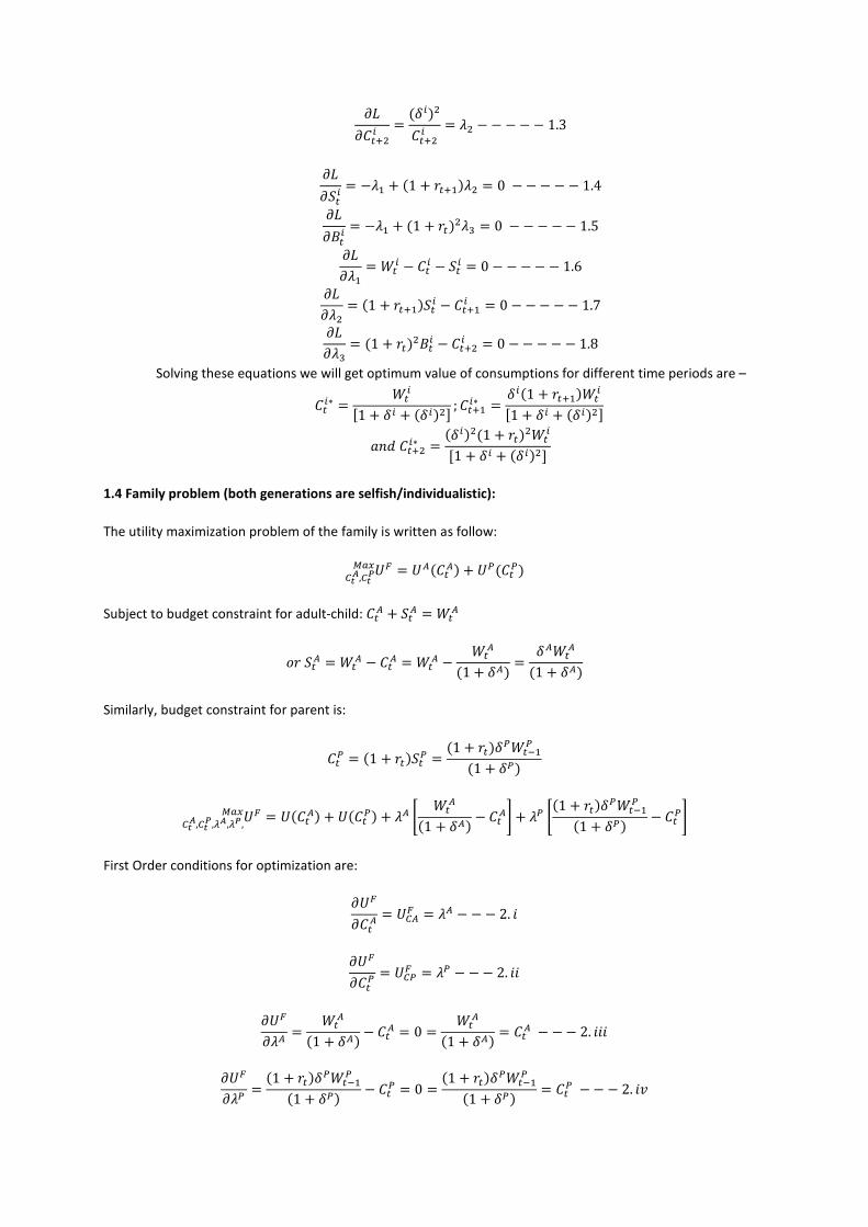
1.4 Family problem (both generations are selfish/individualistic):

The utility maximization problem of the family is written as follow:

"Q��R,��PSTU = "N���N� + "O���O�

Subject to budget constraint for adult-child: ��N + ��N = �N

.� ��N = �N − ��N = �N − �N�1 + �N� = �N �N�1 + �N�

Similarly, budget constraint for parent is:

��O = �1 + �����O = �1 + ����O �5�O�1 + �O�

"Q��R,��P,,R,,P,STU = "���N� + "���O� + XN [ �N�1 + �N� − ��N\ + XO [�1 + ����O �5�O�1 + �O� − ��O\

First Order conditions for optimization are:

�"Q���N

= "�NQ = XN − − − 2. �

�"Q���O

= "�OQ = XO − − − 2. ��

�"Q�XN = �N�1 + �N� − ��N = 0 = �N�1 + �N� = ��N − − − 2. ���

�"Q�XO = �1 + ����O �5�O

�1 + �O� − ��O = 0 = �1 + ����O �5�O�1 + �O� = ��O − − − 2. �/

The marginal rate of substitution (�(���,P��R� between the consumption of two generations is as follows.

"�NQ"�OQ = XN

XO

Logarithmic Utility function:

"Q��R,��P�TU = g���N + g���O

Budget constraint for adult child: ��N + ��N = �N

Budget constraint for parent: ��O = �1 + �����O

Saving function of adult child is

��N = �N �N�1 + �N�

And, saving function of parent is

��O = �O �5�O�1 + �O�

(individual point of view):

wQ��R,��P,!�R,R,,P�TU = ln ��N + g���O + XN � �N − ��N − �N �N�1 + �N�� + XO{�1 + ��� �O �5�O�1 + �O� − ��O}

wQ��R,��P,,R,,P�TU = ln ��N + g���O + XN � �N�1 + �N� − ��N� + XO{�1 + ��� �O �5�O�1 + �O� − ��O}

First Order Conditions are:

�wQ���N

= 1��N

= XN − − − − − 2.1

�wQ���O

= 1��O

= XO − − − −2.2

�wQ�XN = �N�1 + �N� − ��N = 0 − − − 2.3

�wQ�XO = �1 + ��� �O �5�O

�1 + �O� − ��O = 0 − − − −2.4

For adult generation optimum values are:

��N∗ = 1�R���+R� ��� XN∗ = ���+R�

1�R

For parent generation optimum values are:

��O∗ = +P���-��1�H P���+P� ��� XO∗ = ���+P�

+P���-��1�H P

The marginal rate of substitution (MRS) between adult child and parent is : �(��P,�R = ��P∗��R∗ = ,R∗

,P∗ =+P���-��1�H P

%��+P&W1�R %��+R&W

1.5 Utility maximisation of selfish/individualistic joint family- A Social planner’s view:

The family budget constraint is: ��N + ��O = 1�R���+R� + �1 + ��� +P1�H P

%��+P&

"Q��R,��P,,V,STU = "N���N� + "O���O� + XQ [ �N�1 + �N� + �1 + ����O �5�O�1 + �O� − ��N − ��O\

First Order Conditions:

�"Q���N

= "�NQ = XQ − − − 2j. �

�"Q���O

= "�OQ = XQ − − − 2j. ��

�"Q�XQ = �N�1 + �N� + �1 + ����O �5�O

�1 + �O� − ��N − ��O = 0 − − − 2j. ���

For Logarithmic Utility Function:

For a logarithmic utility function, which is additive to get family utility function. The Lagrange Function

becomes as follow:

wQ��R,��P,,V�TU = ln ��N + g���O + XQ � �N�1 + �N� + �1 + ��� �O �5�O�1 + �O� − ��N − ��O�

First Order Conditions for utility maximization are:

�wQ���N

= 1��N

= XQ − − − − − 2j. 1

�wQ���O

= 1��O

= XQ − − − − − 2j. 2

�wQ�XQ = �N�1 + �N� �1 + ��� �O �5�O

�1 + �O� − ��N − ��O = 0 − − − 2j. 3

The optimum value of consumption for each generation as follows.

��N∗ = ��O∗ = �1 + �O� �N + �1 + ����O�1 + �N� �5�O2�1 + �N��1 + �O�

XQ∗ = 2�1 + �N��1 + �O��1 + �O� �N + �1 + ����O�1 + �N� �5�O

1 .6Mono-dimensional Altruism and different marginal utility of money:

The utility function of selfish adult child is: "N = "N���N�

The utility function of altruistic parent is: "O = "O���O� + ^"N���N�

"Q��R,��PSTU = �1 + ^�"N���N� + "O���O�

Subject to budget constraint for adult-child: ��N + ��N = �N + ^

.� ��N = �N + ^ − ��N = �N + ^ − �N�1 + �N� = �N �N�1 + �N� + ^

Similarly, budget constraint for parent is:

��O = �1 + �����O − ^ = �1 + ����O �5�O�1 + �O�

"Q��R,��P,,R,,P,STU = �1 + ^�"N���N� + "O���O� + XN [ �N�1 + �N� + ^ − ��N\ + XO [�1 + ����O �5�O�1 + �O� − ^ − ��O\

First Order conditions for optimization are:

�"Q���N

= �1 + ^�"�NQ = XN − − − 3. �

�"Q���O

= "�OQ = XO − − − 3. ��

�"Q�XN = �N�1 + �N� + ^ − ��N = 0 = �N�1 + �N� + ^ = ��N − − − 3. ���

�"Q�XO = �1 + ����O �5�O

�1 + �O� − ^ − ��O = 0 = �1 + ����O �5�O�1 + �O� − ^ = ��O − −3. �/

The marginal rate of substitution (�(���,P��R� between the consumption of two generations is as

follows. ���`�)*RV)*PV = ,R

,P .� )*RV)*PV = ,R

���`�,P

Logarithmic utility function:

Utility function of adult child: "�N���N� = g���N

Utility function of altruistic Parent: "�O���O� = g���O + ^g���N

Thus the family utility function at time-t is:"�Q = �1 + ^�g���N + g���O

Budget constraint for adult child is: ��N + ��N = �N + ^

When ��N = 1�R���+R� �ℎ8�, ��N = 1�R

���+R� + ^

Budget constraint for altruistic parent is: ��O = �1 + ��� +P1�H P���+P� − ^

wQ��R,��P,,R,,P�TU = �1 + ^�g���N + g���O + XN � �N�1 + �N� + ^−��N� + XO{�1 + ��� �O �5�O�1 + �O� − ^ − ��O}

First Order Conditions are:

�wQ���N

= �1 + ^���N

= XN − − − − − 3.1

�wQ���O

= 1��N

= XO − − − − − 3.2

�wQ�XN = �N�1 + �N� + ^−��N = 0 − − − − − 3.3

�wQ�XO = �1 + ��� �O �5�O

�1 + �O� − ^ − ��O = 0 − − − − − 3.4

The optimum value of consumption and marginal utility of money for adult child generation are:

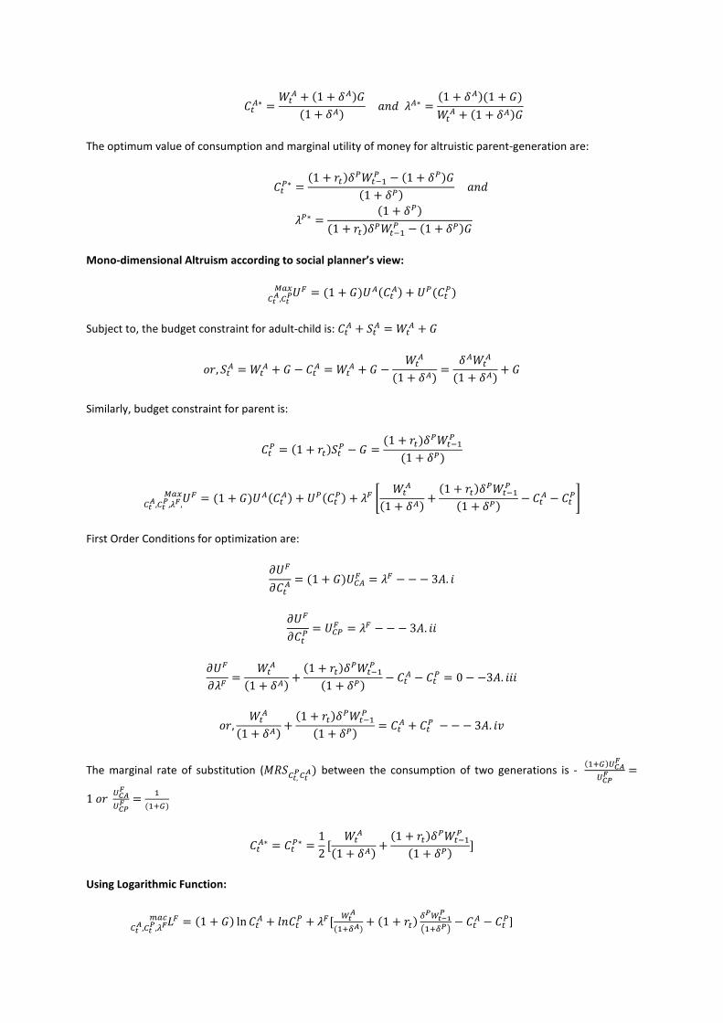
��N∗ = �N + �1 + �N�^�1 + �N� ��� XN∗ = �1 + �N��1 + ^�

�N + �1 + �N�^

The optimum value of consumption and marginal utility of money for altruistic parent-generation are:

��O∗ = �1 + ����O �5�O − �1 + �O�^�1 + �O� ���

XO∗ = �1 + �O��1 + ����O �5�O − �1 + �O�^

Mono-dimensional Altruism according to social planner’s view:

"Q��R,��PSTU = �1 + ^�"N���N� + "O���O�

Subject to, the budget constraint for adult-child is: ��N + ��N = �N + ^

.�, ��N = �N + ^ − ��N = �N + ^ − �N�1 + �N� = �N �N�1 + �N� + ^

Similarly, budget constraint for parent is:

��O = �1 + �����O − ^ = �1 + ����O �5�O�1 + �O�

"Q��R,��P,,V,STU = �1 + ^�"N���N� + "O���O� + XQ [ �N�1 + �N� + �1 + ����O �5�O�1 + �O� − ��N − ��O\

First Order Conditions for optimization are:

�"Q���N

= �1 + ^�"�NQ = XQ − − − 3j. �

�"Q���O

= "�OQ = XQ − − − 3j. ��

�"Q�XQ = �N�1 + �N� + �1 + ����O �5�O

�1 + �O� − ��N − ��O = 0 − −3j. ���

.�, �N�1 + �N� + �1 + ����O �5�O�1 + �O� = ��N + ��O − − − 3j. �/

The marginal rate of substitution (�(���,P��R� between the consumption of two generations is - ���`�)*RV)*PV =

1 .� )*RV)*PV = �

���`�

��N∗ = ��O∗ = 12 [ �N�1 + �N� + �1 + ����O �5�O

�1 + �O� ]

Using Logarithmic Function:

wQ��R,��P,,V�T� = �1 + ^� ln ��N + g���O + XQ[ 1�R���+R� + �1 + ��� +P1�H P

%��+P& − ��N − ��O]

First Order Conditions are:

�wQ���N

= �1 + ^���N

= XQ − − − − − −3.1.1

�wQ���O

= 1��O

= XQ − − − − − −3.1.2

�wQ�XQ = �N�1 + �N� + �1 + ��� �O �5�O

�1 + �O� − ��N − ��O = 0 − − − − − −3.1.3

⇒ �N�1 + �N� + �1 + ��� �O �5�O�1 + �O� = 2 + ^

XQ

XQ∗ = �2 + ^��1 + �N��1 + �O��1 + �O� �N + �1 + ����O�1 + �N� �5�O

Optimum value of consumption for adult child is:

��N∗ = �1 + ^�[�1 + �O� �N + �1 + ����O�1 + �N� �5�O ]�2 + ^��1 + �N��1 + �O�

Optimum value of consumption for altruistic parent is:

��O∗ = [�1 + �O� �N + �1 + ����O�1 + �N� �5�O ]�2 + ^��1 + �N��1 + �O�

1.8 A Duo-Dimensional Altruistic joint family with different marginal utility of money:

The utility function of child is: "�N = "N���N� + j"�O

The utility function of parent is: "�O = "O���O� + ^"�N

The utility function of child is: "�N = "N���N� + j"O���O�

The utility function of child is: "�O = "O���O� + ^"N���N�

Assuming additive utility, family function becomes –

"Q = �1 + ^�"N���N� + �1 + j�"O���O�

Budget constraint for child generation: ��N + ��N + j = �N + ^

Or, ��N = 1�R���+R� + ^ − j

Budget constraint for parent generation: ��O + ^ = �1 + ��� +P1�H P���+P� + j

"Q��R,��P,,R,,PSTU = �1 + ^�"N���N� + �1 + j�"O���O� + XN [ �N�1 + �N� + ^ − j − ��N\ + XO[�1 + ��� �O �5�O�1 + �O�

+ j − ^ − ��O]

First Order Conditions are:

�"Q���N

= �1 + ^�"�NQ = XN − − − 4. �

�"Q���O

= �1 + j�"�OQ = XO − − − 4. ��

�"Q�XN = [ �N�1 + �N� + ^ − j − ��N\ = 0 − −4. ���

��N∗ = �N�1 + �N� + ^ − j

�"Q�XO = �1 + ��� �O �5�O

�1 + �O� + j − ^ − ��O = 0 − −4. �/

��O∗ = �1 + ��� �O �5�O�1 + �O� + j − ^

The marginal rate of substitution (�(���,P��R� between the consumption of two generations is - ���`�)*RV���N�)*PV =

,R,P = )*RV

)*PV = ���N�,R���`�,P

Logarithmic utility function:

"��g��i fc�e��.� f.� ��cg�: "N = g���N + jg���O

And,

"��g��i fc�e��.� f.� L��8��: "O = g���O + ^g���N

Budget constraint for adult generation: ��N + ��N + j = �N + ^

Or, ��N = 1�R���+R� + ^ − j

Budget constraint for parent generation: ��O + ^ = �1 + ��� +P1�H P���+P� + j

The family utility function becomes,

"Q = �1 + ^�g���N + �1 + j�g���O

wQ = �1 + ^�g���N + �1 + j�g���O + XN [ �N�1 + �N� + ^ − j − ��N\ + XO[�1 + ��� �O �5�O�1 + �O� + j − ^ − ��O]

First Order Conditions are:

�wQ���N

= �1 + ^���N

= XN − − − − − − − 4.1

�wQ���O

= �1 + j���O

= XO − − − − − − − 4.2

�wQ�XN = �N�1 + �N� + ^ − j − ��N = 0 − − − − − − − 4.3

�N�1 + �N� + ^ − j = ��N − − − −4.3�

�wQ�XO = �1 + ��� �O �5�O

�1 + �O� + j − ^ − ��O = 0 − − − − − − − 4.4

�1 + ��� �O �5�O�1 + �O� + j − ^ = ��O − − − −4.4�

The marginal rate of substitution between two generations is

�(��P,�R =�1 + ^� ��NW�1 + j� ��OW = XN

XO − − − −4.5

After mathematical manipulation we get the optimum values of consumptions and marginal utility of money

are as follows.

��N∗ = XO�1 + ^��1 + ����O �5�OXN�1 + j��1 + �O� + XO�1 + ^��j − ^�

XN�1 + j�

��O∗ = XN�1 + j� �NXO�1 + ^��1 + �N� + XN�1 + j��^ − j�XO�1 + ^�

Optimum marginal utility of money for adult-child is

XN∗ = �1 + ^��1 + �N� �N + �1 + �N��^ − j�

Optimum marginal utility of money for parent is

XO∗ = �1 + j��1 + �O��1 + ����O �5�O + �1 + �O��j − ^�

4A.Family Behaviour with Two Dimensional Altruisms having same Marginal Utility of Money (Social Planner

Point of View):

"Q��R,��P,,V,STU = �1 + ^�"N���N� + �1 + j�"O���O� + XQ [ �N�1 + �N� + �1 + ��� �O �5�O�1 + �O� − ��N − ��O\

First Order Conditions are:

�"Q���N

= �1 + ^�"�NQ = XQ − − − 4j. �

�"Q���O

= �1 + j�"�OQ = XQ − − − 4j. ��

�"Q�XQ = [ �N�1 + �N� + �1 + ��� �O �5�O

�1 + �O� − ��N − ��O\ = 0 − −4j. �/

��N + ��O = �N�1 + �N� + �O �5�O�1 + �O�

The marginal rate of substitution (�(���,P��R� between the consumption of two generations is - ���`�)*RV���N�)*PV =

1 = )*RV)*PV = ���N�

���`�.

��N∗ = ��O∗ = 12 [ �N�1 + �N� + �O �5�O

�1 + �O�]

Logarithmic utility function:

"��g��i fc�e��.� f.� ��cg�: "N = g���N + jg���O

And,

"��g��i fc�e��.� f.� L��8��: "O = g���O + ^g���N

Budget constraint for adult generation: ��N + ��N + j = �N + ^

Or, ��N = 1�R���+R� + ^ − j

Budget constraint for parent generation: ��O + ^ = �1 + ��� +P1�H P���+P� + j

The family utility function becomes,

"Q = �1 + ^�g���N + �1 + j�g���O

Now the marginal utility of money is same for both generations, so the Lagrange function can be written as

follow:

wQ = �1 + ^�g���N + �1 + j�g���O + XQ[ �N�1 + �N� + �1 + ��� �O �5�O�1 + �O� − ��N − ��O]

First Order Conditions:

�wQ���N

= �1 + ^���N

= XQ − − − − − − − −7.1

�wQ���O

= �1 + j���O

= XQ − − − − − − − −7.2

�wQ�XQ = �N�1 + �N� + �1 + ��� �O �5�O

�1 + �O� − ��N − ��O = 0 − − − − − − − 7.3

Solving equations 7.1, 7.2 and 7.3 we get the marginal utility of money for both generations is as follows:

XQ = �2 + ^ + j��1 + �N��1 + �O��1 + �O� �N + �1 + ����O�1 + �N� �5�O

The optimal consumption of altruistic adult generation is as follows:

��N = �1 + ^��1 + �O� �N + �1 + ����O�1 + �N� �5�O�2 + ^ + j��1 + �N��1 + �O�

The optimal consumption of altruistic old (parent) generation is as follows:

��O = �1 + j��1 + �O� �N + �1 + ����O�1 + �N� �5�O�2 + ^ + j��1 + �N��1 + �O�

Table 1

Living Arrangement of Elderly Population (aged 60 and above) by Selected Regions and Sub-regions

of the World

Living Arrangement

Region/Subregion

Alone

Couple

only

With

children or

grandchildr

en

With other

relatives or

nonrelatives

Total

Asia 7 16 74 4 100

East 9 20 70 1 100

▪Southeast 6 13 73 9 100

South-central 4 9 83 - 100

Africa 8 9 74 8

Europe 26 43 26 4 100

South 19 39 38 4 100

Latin America &

Caribbean

9 16 62 14 100

North America 26 47 19 8 100

Source: UN 2005, Table II.5, p 36

Table-2: The dependent variable is percentage of elderly men living with a child or grandchild

(PECPM)

Const.

Co-efft. Co-efft.

of PGDP Co-

efft.

of

PSMP

Co-

efft.

of

APG

R

Co-

efft. of

PUPN

Co-efft.

of AFRI Co-efft.

of ASIA Co-

efft.

of

EUR

O

Co-efft.

of

LTAM

Co-

efft.

of

LDEV

Co-

efft.

of

NDE

V

(9

Value

32.37�14.030�∗ −0.0005�0.0004�

∗

45.79�12.60�∗∗ 48.48�12.29�

∗∗ 2.78

(10.7

8)

38.00�12.20�∗∗ −0.85�6.94�

∗ −3.75�5.57�∗

0.85

(std.e

rr)

33.38�15.05�∗∗∗ −0.0005�0.0004�

∗ −0.07 �0.20�

45.43�8.24�∗∗∗ 48.37�8.12�

∗∗∗ 2.48

(6.50

)

37.54�7.71�∗∗∗ −1.31�9.65�

∗ −4.10�7.66�∗

0.85

(std.e

rr)

31.55�13.06�∗∗∗ −0.0006�0.0004�

∗

4.06∗∗ �1.71� 35.12�8.28�∗∗∗ 43.04�7.70�

∗∗∗ 4.98

(6.03

)

30.91�7.23�∗∗∗ −0.40�8.5�

∗ −1.94�6.91�∗

0.87

(std.e

rr)

38.30�12.70�∗∗∗ −0.00046�0.00044� −0.21�0.08�

∗∗ 45.98�7.38�∗∗∗ 50.33�7.47�

∗∗∗ 3.66

(5.75

)

42.63�6.65�∗∗∗ −5.31�9.44�

∗ −5.02�7.51�∗

0.86

(std.e

rr)

32.35�13.79�∗∗∗ −0.0006�0.0004�

∗ −0.05 �0.15�

4.05∗∗∗�1.70� 34.86�8.70�

∗∗∗ 42.97�7.91�∗∗∗ 4.74

(6.17

)

30.57�7.79�∗∗∗ −0.77�8.75�

∗ −2.23�7.01�∗

0.87

(std.e

rr)

42.46�14.05�∗∗∗ −0.0003�0.0004�

∗ 0.094 �0.21�

−0.22�0.07�∗∗ 46.53�7.73�

∗∗∗ 50.65�7.67�∗∗∗ 4.19

(6.04

)

43.71�7.66�∗∗∗ −5.04�9.42�

∗ −4.61�7.48�∗

0.86

(std.e

rr)

38.52�12.51�∗∗∗ −0.0005�0.0004�

∗

3.44∗∗∗�1.72� −0.13�0.07�

∗∗ 36.86�8.15�∗∗∗ 45.06�7.64�

∗∗∗ 5.21

(5.77

)

34.97�7.32�∗∗∗ −3.35�8.41�

∗ −3.03�6.93�∗

0.88

(std.e

rr)

38.30�12.70�∗∗∗ −0.00046�0.00044� 0.048 �0.179�

3.40∗∗ �1.89� −0.14�0.08�∗∗ 37.24�8.90�

∗∗∗ 45.28�8.09�∗∗∗ 2.48

(6.50

)

35.61�8.69�∗∗∗ −3.23�8.46�

∗ −2.85�6.94�∗

0.88

(std.e

rr)

• *Indicates expected sign but not significant.

** Indicates expected sign and significant at 10% error level.

*** Indicates expected sign and significant at 5% error level.

Table-3: The dependent variable is percentage of elderly women living with a child or grandchild

(PECPW)

Const.

Co-efft. Co-efft.

of PGDP Co-

efft.

of

PSMP

Co-

efft.

of

APG

R

Co-

efft. of

PUPN

Co-

efft. of

AFRI

Co-

efft. of

ASIA

Co-

efft.

of

EUR

O

Co-

efft. of

LTAM

Co-

efft.

of

LDEV

Co-

efft.

of

NDEV

(9

Value

48.18�12.71�∗∗ −0.00095�0.0004�

∗∗

34.08�7.43�∗∗ 39.24�7.25�

∗∗ −4.40(5.8

9)

30.17�6.70�∗∗ −9.72�8.22�

∗

−6.10�6.66�∗

0.87

(std.e

rr)

40.75�13.47�∗∗ −0.00095�0.0004�

∗∗ −0.36 �0.14�

33.88�7.76�∗∗ 39.19�7.44�

∗∗ −4.58(6.0

3)

29.92�7.12�∗∗ −9.98�8.50�

∗

−6.30�6.84�∗

0.87

(std.e

rr)

47.69�12.50�∗∗ −0.001�0.0004�

∗∗∗

2.44∗∗∗�1.05�

27.67�8.38�∗∗ 35.97�7.55�

∗∗ −3.09(5.8

1)

25.91�7.14�∗∗ −9.45�8.17�

∗

−5.01�6.61�∗

0.87

(std.e

rr)

55.96�12.07�∗∗ −0.0008�0.0004�

∗∗∗ −0.15�0.07�

∗∗∗ 34.22�7.37�∗∗ 40.80�7.22�

∗∗ −3.76(5.5

4)

33.57�6.82�∗∗ −12.99�8.26�

∗ −7.03�6.73�∗

0.87

(std.e

rr)

48.13�13.12�∗∗ −0.001�0.0004�

∗∗∗ −0.03 �0.13�

2.43∗∗∗�1.03�

27.52�8.58�∗∗ 35.93�7.67�

∗∗ −3.

22

(5.9

1)

25.72�7.41�∗∗ −9.66�8.46�

∗

−5.17�6.84�∗

0.88

(std.e

rr)

55.51�12.24�∗∗ −0.0008�0.0004�

∗∗∗ 0.08 �0.16�

−0.17�0.07�∗∗∗ 34.69�7.52�

∗∗ 40.88�7.27�∗∗ −3.31

(5.7

3)

34.51�7.40�∗∗ −12.76�8.31�

∗ −6.68�6.78�∗

0.87

(std.e

rr)

53.46�11.84�∗∗ −0.0009�0.0004�

∗∗∗ 1.93∗∗ �1.05�

−0.11�0.065�∗ 29.11�8.38�

∗∗ 37.64�7.62�∗∗ −2.89

(5.5

4)

29.27�7.43�∗∗ −11.9�8.09�

∗

−5.92�6.67�∗

0.88

(std.e

rr)

53.21�11.90�∗∗ −0.0009�0.00042�

∗ 0.057 �0.159�

1.89∗∗ �1.12�

−0.12

(0.08)

29.55�8.78�∗∗ 37.90�7.79�

∗∗ −2.59(5.7

2)

30.02�8.24�∗∗ −11.76�8.18�

∗ −5.70�6.77�∗

0.88

(std.e

rr)

• *Indicates expected sign but not significant.

** Indicates expected sign and significant at 10% error level.

*** Indicates expected sign and significant at 5% error level.