Embed Size (px)
Citation preview
74
Chapter 2
Functions and Their Graphs Section 2.1
1. ( )1,3−
2. ( ) ( ) ( ) ( ) ( )2
12
1 13 2 5 2 3 4 5 22 2
112 102
43 or 212
− − − + = − − −−
= + −
=
3. We must not allow the denominator to be 0. 4 0 4x x+ ≠ ⇒ ≠ − ; Domain: { }4x x ≠ − .
4. 3 2 52 2
1
xxx
− >− >
< −
Solution set: { }| 1x x < − or ( ), 1−∞ −
−1 0
5. independent; dependent
6. range
7. [ ]0,5
We need the intersection of the intervals [ ]0,7
and [ ]2,5− .
7−2 50
7−2 50
7−2 50
f
g
f + g
8. ≠ ; ( )f x ; ( )g x
9. ( ) ( )g x f x− , or ( )( )g f x−
10. False; every function is a relation, but not every relation is a function. For example, the relation
2 2 1x y+ = is not a function.
11. True
12. True
13. False; if the domain is not specified, we assume it is the largest set of real numbers for which the value of f is a real number.
14. False; the domain of ( )2 4xf xx−
= is
{ }| 0x x ≠ .
15. Function Domain: {Elvis, Colleen, Kaleigh, Marissa} Range: {Jan. 8, Mar. 15, Sept. 17}
16. Not a function
17. Not a function
18. Function Domain: {Less than 9th grade, 9th-12th grade,
High School Graduate, Some College, College Graduate}
Range: {$18,120, $23,251, $36,055, $45,810, $67,165}
19. Not a function
20. Function Domain: {–2, –1, 3, 4} Range: {3, 5, 7, 12}
21. Function Domain: {1, 2, 3, 4} Range: {3}
22. Function Domain: {0, 1, 2, 3} Range: {–2, 3, 7}
23. Not a function
24. Not a function
25. Function Domain: {–2, –1, 0, 1} Range: {0, 1, 4}
26. Function Domain: {–2, –1, 0, 1} Range: {3, 4, 16}

ISM: Precalculus EGU Chapter 2: Functions and Their Graphs
75
27. Graph 2y x= . The graph passes the vertical line test. Thus, the equation represents a function.
28. Graph 3y x= . The graph passes the vertical line test. Thus, the equation represents a function.
29. Graph 1yx
= . The graph passes the vertical line
test. Thus, the equation represents a function.
30. Graph y x= . The graph passes the vertical line test. Thus, the equation represents a function.
31. 2 24y x= −
Solve for 2: 4y y x= ± − For 0, 2x y= = ± . Thus, (0, 2) and (0, –2) are on the graph. This is not a function, since a distinct x corresponds to two different y 's.
32. 1 2y x= ± − For 0, 1x y= = ± . Thus, (0, 1) and (0, –1) are on the graph. This is not a function, since a distinct x corresponds to two different y 's.
33. 2x y=
Solve for :y y x= ± For 1, 1x y= = ± . Thus, (1, 1) and (1, –1) are on the graph. This is not a function, since a distinct x corresponds to two different y 's.
34. 2 1x y+ =
Solve for : 1y y x= ± − For 0, 1x y= = ± . Thus, (0, 1) and (0, –1) are on the graph. This is not a function, since a distinct x corresponds to two different y 's.
35. Graph 22 3 4y x x= − + . The graph passes the vertical line test. Thus, the equation represents a function.
36. Graph 3 12
xyx−
=+
. The graph passes the vertical
line test. Thus, the equation represents a function.
37. 2 22 3 1x y+ =
Solve for y: 2 2
2 2
22
2
2 3 1
3 1 2
1 23
1 23
x y
y x
xy
xy
+ =
= −
−=
−= ±
For 10,3
x y= = ± . Thus, 10,3
⎛ ⎞⎜ ⎟⎜ ⎟⎝ ⎠
and
10,3
⎛ ⎞−⎜ ⎟⎜ ⎟
⎝ ⎠are on the graph. This is not a
function, since a distinct x corresponds to two different y 's.

Chapter 2: Functions and Their Graphs ISM: Precalculus EGU
76
38. 2 24 1x y− =
Solve for y: 2 2
2 2
22
2
4 1
4 1
14
12
x y
y x
xy
xy
− =
= −
−=
± −=
For 12,2
x y= = ± . Thus, 12,2
⎛ ⎞⎜ ⎟⎝ ⎠
and
12,2
⎛ ⎞−⎜ ⎟⎝ ⎠
are on the graph. This is not a
function, since a distinct x corresponds to two different y 's.
39. ( ) 23 2 4f x x x= + −
a. ( ) ( ) ( )20 3 0 2 0 4 4f = + − = −
b. ( ) ( ) ( )21 3 1 2 1 4 3 2 4 1f = + − = + − =
c. ( ) ( ) ( )21 3 1 2 1 4 3 2 4 3f − = − + − − = − − = −
d. ( ) ( ) ( )2 23 2 4 3 2 4f x x x x x− = − + − − = − −
e. ( ) ( )2 23 2 4 3 2 4f x x x x x− = − + − = − − +
f. ( ) ( ) ( )( )
2
2
2
2
1 3 1 2 1 4
3 2 1 2 2 4
3 6 3 2 2 4
3 8 1
f x x x
x x x
x x x
x x
+ = + + + −
= + + + + −
= + + + + −
= + +
g. ( ) ( ) ( )2 22 3 2 2 2 4 12 4 4f x x x x x= + − = + −
h. ( ) ( ) ( )( )
2
2 2
2 2
3 2 4
3 2 2 2 4
3 6 3 2 2 4
f x h x h x h
x xh h x h
x xh h x h
+ = + + + −
= + + + + −
= + + + + −
40. ( ) 22 1f x x x= − + −
a. ( ) ( )20 2 0 0 1 1f = − + − = −
b. ( ) ( )21 2 1 1 1 2f = − + − = −
c. ( ) ( ) ( )21 2 1 1 1 4f − = − − + − − = −
d. ( ) ( ) ( )2 22 1 2 1f x x x x x− = − − + − − = − − −
e. ( ) ( )2 22 1 2 1f x x x x x⎡ ⎤− = − − + − = − +⎣ ⎦
f. ( ) ( ) ( )( )
2
2
2
2
1 2 1 1 1
2 2 1 1 1
2 4 2
2 3 2
f x x x
x x x
x x x
x x
+ = − + + + −
= − + + + + −
= − − − +
= − − −
g. ( ) ( ) ( )2 22 2 2 2 1 8 2 1f x x x x x= − + − = − + −
h. ( ) ( )( )
2
2 2
2 2
2( ) 1
2 2 1
2 4 2 1
f x h x h x h
x xh h x h
x xh h x h
+ = − + + + −
= − + + + + −
= − − − + + −
41. ( ) 2 1xf x
x=
+
a. ( ) 20 00 0
10 1f = = =
+
b. ( ) 21 11
21 1f = =
+
c. ( )( )2
1 1 111 1 21 1
f − −− = = = −
+− +
d. ( )( )2 2 11
x xf xxx
− −− = =
+− +
e. ( ) 2 21 1x xf x
x x−⎛ ⎞− = − =⎜ ⎟+ +⎝ ⎠
f. ( )( )2
2
2
111 1
12 1 1
12 2
xf xx
xx x
xx x
++ =
+ +
+=
+ + ++
=+ +
g. ( )( )2 2
2 224 12 1
x xf xxx
= =++
h. ( )( )2 2 22 11
x h x hf x hx xh hx h
+ ++ = =
+ + ++ +
42. ( )2 1
4xf xx−
=+
a. ( )20 1 1 10
0 4 4 4f − −
= = = −+

ISM: Precalculus EGU Chapter 2: Functions and Their Graphs
77
b. ( )21 1 01 0
1 4 5f −
= = =+
c. ( ) ( )21 1 01 01 4 3
f− −
− = = =− +
d. ( ) ( )2 21 14 4
x xf xx x
− − −− = =
− + − +
e. ( )2 21 1
4 4x xf xx x
⎛ ⎞− −− = − =⎜ ⎟⎜ ⎟+ +⎝ ⎠
f. ( ) ( )( )
2 2
2
1 1 2 1 111 4 5
25
x x xf xx x
x xx
+ − + + −+ = =
+ + +
+=
+
g. ( ) ( )2 22 1 4 122 4 2 4x xf xx x
− −= =
+ +
h. ( ) ( )( )
2 2 21 2 14 4
x h x xh hf x hx h x h+ − + + −
+ = =+ + + +
43. ( ) 4f x x= +
a. ( )0 0 4 0 4 4f = + = + =
b. ( )1 1 4 1 4 5f = + = + =
c. ( )1 1 4 1 4 5f − = − + = + =
d. ( ) 4 4f x x x− = − + = +
e. ( ) ( )4 4f x x x− = − + = − −
f. ( )1 1 4f x x+ = + +
g. ( )2 2 4 2 4f x x x= + = +
h. ( ) 4f x h x h+ = + +
44. ( ) 2f x x x= +
a. ( ) 20 0 0 0 0f = + = =
b. ( ) 21 1 1 2f = + =
c. ( ) ( ) ( )21 1 1 1 1 0 0f − = − + − = − = =
d. ( ) ( ) ( )2 2f x x x x x− = − + − = −
e. ( ) ( )2 2f x x x x x− = − + = − +
f. ( ) ( ) ( )2
2
2
1 1 1
2 1 1
3 2
f x x x
x x x
x x
+ = + + +
= + + + +
= + +
g. ( ) ( )2 22 2 2 4 2f x x x x x= + = +
h. ( ) ( ) ( )2
2 22
f x h x h x h
x xh h x h
+ = + + +
= + + + +
45. ( ) 2 13 5
xf xx+
=−
a. ( ) ( )( )
2 0 1 0 1 103 0 5 0 5 5
f+ +
= = = −− −
b. ( ) ( )( )
2 1 1 2 1 3 313 1 5 3 5 2 2
f+ +
= = = = −− − −
c. ( ) ( )( )
2 1 1 2 1 1 113 1 5 3 5 8 8
f− + − + −
− = = = =− − − − −
d. ( ) ( )( )
2 1 2 1 2 13 5 3 5 3 5
x x xf xx x x− + − + −
− = = =− − − − +
e. ( ) 2 1 2 13 5 3 5
x xf xx x+ − −⎛ ⎞− = − =⎜ ⎟− −⎝ ⎠
f. ( ) ( )( )
2 1 1 2 2 1 2 313 1 5 3 3 5 3 2
x x xf xx x x+ + + + +
+ = = =+ − + − −
g. ( ) ( )( )
2 2 1 4 123 2 5 6 5
x xf xx x
+ += =
− −
h. ( ) ( )( )
2 1 2 2 13 5 3 3 5
x h x hf x hx h x h+ + + +
+ = =+ − + −
46. ( )( )2
112
f xx
= −+
a. ( )( )2
1 1 30 1 14 40 2
f = − = − =+
b. ( )( )2
1 1 81 1 19 91 2
f = − = − =+

Chapter 2: Functions and Their Graphs ISM: Precalculus EGU
78
c. ( )( )2
1 11 1 1 011 2
f − = − = − =− +
d. ( )( ) ( )2 2
1 11 12 2
f xx x
− = − = −− + −
e. ( )( ) ( )2 2
1 11 12 2
f xx x
⎛ ⎞⎜ ⎟− = − − = −⎜ ⎟+ +⎝ ⎠
f. ( )( ) ( )2 2
1 11 1 11 2 3
f xx x
+ = − = −+ + +
g. ( )( ) ( )2 2
1 12 1 12 2 4 1
f xx x
= − = −+ +
h. ( )( )2
112
f x hx h
+ = −+ +
47. ( ) 5 4f x x= − +
Domain: { } is any real numberx x
48. 2( ) 2f x x= +
Domain: { } is any real numberx x
49. 2( )1
xf xx
=+
Domain: { } is any real numberx x
50. 2
2( )1
xf xx
=+
Domain: { } is any real numberx x
51. 2( )16
xg xx
=−
2
2
16 0
16 4
x
x x
− ≠
≠ ⇒ ≠ ±
Domain: { }4, 4x x x≠ − ≠
52. 22( )
4xh x
x=
−
2
2
4 0
4 2
x
x x
− ≠
≠ ⇒ ≠ ±
Domain: { }2, 2x x x≠ − ≠
53. 32( ) xF x
x x−
=+
3
2
2
0
( 1) 0
0, 1
x x
x x
x x
+ ≠
+ ≠
≠ ≠ −
Domain: { }0x x ≠
54. 34( )4
xG xx x
+=
−
3
2
2
4 0
( 4) 0
0, 40, 2
x x
x x
x xx x
− ≠
− ≠
≠ ≠≠ ≠ ±
Domain: { }0, 2, 2x x x x≠ ≠ ≠ −
55. ( ) 3 12h x x= − 3 12 0
3 124
xxx
− ≥≥≥
Domain: { }4x x ≥
56. ( ) 1G x x= − 1 0
11
xxx
− ≥− ≥ −
≤
Domain: { }1x x ≤
57. 4( )9
f xx
=−
9 09
xx
− >>
Domain: { }9x x >
58. ( )4
xf xx
=−
4 04
xx
− >>
Domain: { }4x x >

ISM: Precalculus EGU Chapter 2: Functions and Their Graphs
79
59. 2 2( )1 1
p xx x
= =− −
1 01
xx
− >>
Domain: { }1x x >
60. ( ) 2q x x= − − 2 0
22
xxx
− − ≥− ≥
≤ −
Domain: { }2x x ≤ −
61. ( ) 3 4 ( ) 2 3f x x g x x= + = −
a. ( )( ) 3 4 2 3 5 1f g x x x x+ = + + − = +
The domain is { } is any real numberx x .
b. ( )( ) (3 4) (2 3)3 4 2 3
7
f g x x xx x
x
− = + − −= + − += +
The domain is { } is any real numberx x .
c. 2
2
( )( ) (3 4)(2 3)
6 9 8 12
6 12
f g x x x
x x x
x x
⋅ = + −
= − + −
= − −
The domain is { } is any real numberx x .
d. 3 4( )2 3
f xxg x
⎛ ⎞ +=⎜ ⎟ −⎝ ⎠
32 3 0 2 32
x x x− ≠ ⇒ ≠ ⇒ ≠
The domain is 32
x x⎧ ⎫≠⎨ ⎬
⎩ ⎭.
62. ( ) 2 1 ( ) 3 2f x x g x x= + = −
a. ( )( ) 2 1 3 2 5 1f g x x x x+ = + + − = −
The domain is { } is any real numberx x .
b. ( )( ) (2 1) (3 2)2 1 3 2
3
f g x x xx xx
− = + − −= + − += − +
The domain is { } is any real numberx x .
c. 2
2
( )( ) (2 1)(3 2)
6 4 3 2
6 2
f g x x x
x x x
x x
⋅ = + −
= − + −
= − −
The domain is { } is any real numberx x .
d. 2 1( )3 2
f xxg x
⎛ ⎞ +=⎜ ⎟ −⎝ ⎠
3 2 023 23
x
x x
− ≠
≠ ⇒ ≠
The domain is 23
x x⎧ ⎫≠⎨ ⎬
⎩ ⎭.
63. 2( ) 1 ( ) 2f x x g x x= − =
a. 2 2( )( ) 1 2 2 1f g x x x x x+ = − + = + −
The domain is { } is any real numberx x .
b. 2
2
2
( )( ) ( 1) (2 )
1 2
2 1
f g x x x
x x
x x
− = − −
= − −
= − + −
The domain is { } is any real numberx x .
c. 2 3 2( )( ) ( 1)(2 ) 2 2f g x x x x x⋅ = − = −
The domain is { } is any real numberx x .
d. 21( )
2f xxg x
⎛ ⎞ −=⎜ ⎟
⎝ ⎠
The domain is { }0x x ≠ .
64. 2 3( ) 2 3 ( ) 4 1f x x g x x= + = +
a. 2 3
3 2
( )( ) 2 3 4 1
4 2 4
f g x x x
x x
+ = + + +
= + +
The domain is { } is any real numberx x .
b. ( ) ( )2 3
2 3
3 2
( )( ) 2 3 4 1
2 3 4 1
4 2 2
f g x x x
x x
x x
− = + − +
= + − −
= − + +
The domain is { } is any real numberx x .
c. ( )( )2 3
5 3 2
( )( ) 2 3 4 1
8 12 2 3
f g x x x
x x x
⋅ = + +
= + + +
The domain is { } is any real numberx x .

Chapter 2: Functions and Their Graphs ISM: Precalculus EGU
80
d. 2
32 3( )4 1
f xxg x
⎛ ⎞ +=⎜ ⎟
+⎝ ⎠
3
3
33 3
4 1 0
4 1
1 1 24 4 2
x
x
x x
+ ≠
≠ −
≠ − ⇒ ≠ − = −
The domain is 3 22
x x⎧ ⎫⎪ ⎪≠ −⎨ ⎬⎪ ⎪⎩ ⎭
.
65. ( ) ( ) 3 5f x x g x x= = −
a. ( )( ) 3 5f g x x x+ = + −
The domain is { }0x x ≥ .
b. ( )( ) (3 5) 3 5f g x x x x x− = − − = − +
The domain is { }0x x ≥ .
c. ( )( ) (3 5) 3 5f g x x x x x x⋅ = − = −
The domain is { }0x x ≥ .
d. ( )3 5
f xxg x
⎛ ⎞=⎜ ⎟ −⎝ ⎠
0 and 3 5 05 3 53
x x
x x
≥ − ≠
≠ ⇒ ≠
The domain is 50 and 3
x x x⎧ ⎫≥ ≠⎨ ⎬
⎩ ⎭.
66. ( ) ( )f x x g x x= =
a. ( )( )f g x x x+ = +
The domain is { } is any real numberx x .
b. ( )( )f g x x x− = −
The domain is { } is any real numberx x .
c. ( )( )f g x x x⋅ = ⋅
The domain is { } is any real numberx x .
d. ( )xf x
g x⎛ ⎞
=⎜ ⎟⎝ ⎠
The domain is { }0x x ≠ .
67. 1 1( ) 1 ( )f x g xx x
= + =
a. 1 1 2( )( ) 1 1f g xx x x
+ = + + = +
The domain is { }0x x ≠ .
b. 1 1( )( ) 1 1f g xx x
− = + − =
The domain is { }0x x ≠ .
c. 21 1 1 1( )( ) 1f g xx x x x
⎛ ⎞⋅ = + = +⎜ ⎟⎝ ⎠
The domain is { }0x x ≠ .
d.
1 11 1( ) 11 1 1
xf x xx xx xg x
x x
++⎛ ⎞ +
= = = ⋅ = +⎜ ⎟⎝ ⎠
The domain is { }0x x ≠ .
68. ( ) 2 ( ) 4f x x g x x= − = −
a. ( )( ) 2 4f g x x x+ = − + − 2 0 and 4 0
2 and 4 4
x xx x
x
− ≥ − ≥≥ − ≥ −
≤
The domain is { } 2 4x x≤ ≤ .
b. ( )( ) 2 4f g x x x− = − − − 2 0 and 4 0
2 and 4 4
x xx x
x
− ≥ − ≥≥ − ≥ −
≤
The domain is { } 2 4x x≤ ≤ .
c. ( )( )2
( )( ) 2 4
6 8
f g x x x
x x
⋅ = − −
= − + −
2 0 and 4 0 2 and 4 4
x xx x
x
− ≥ − ≥≥ − ≥ −
≤
The domain is { } 2 4x x≤ ≤ .

ISM: Precalculus EGU Chapter 2: Functions and Their Graphs
81
d. 2( )4
f xxg x
⎛ ⎞ −=⎜ ⎟
−⎝ ⎠
2 0 and 4 0 2 and 4 4
x xx x
x
− ≥ − >≥ − > −
<
The domain is { } 2 4x x≤ < .
69. 2 3 4( ) ( )3 2 3 2
x xf x g xx x+
= =− −
a. 2 3 4( )( )3 2 3 22 3 4
3 26 33 2
x xf g xx xx x
xxx
++ = +
− −+ +
=−
+=
−
23
3 2 0
3 2
x
x x
− ≠
≠ ⇒ ≠
The domain is { }23x x ≠ .
b. 2 3 4( )( )3 2 3 22 3 4
3 22 3
3 2
x xf g xx xx x
xx
x
+− = −
− −+ −
=−
− +=
−
3 2 023 23
x
x x
− ≠
≠ ⇒ ≠
The domain is 23
x x⎧ ⎫≠⎨ ⎬
⎩ ⎭.
c. 2
22 3 4 8 12( )( )3 2 3 2 (3 2)
x x x xf g xx x x+ +⎛ ⎞⎛ ⎞⋅ = =⎜ ⎟⎜ ⎟− − −⎝ ⎠⎝ ⎠
3 2 023 23
x
x x
− ≠
≠ ⇒ ≠
The domain is 23
x x⎧ ⎫≠⎨ ⎬
⎩ ⎭.
d.
2 32 3 3 2 2 33 2( )
4 3 2 4 43 2
xf x x xxx
xg x x xx
+⎛ ⎞ + − +−= = ⋅ =⎜ ⎟ −⎝ ⎠
−
3 2 0 and 03 2
23
x xx
x
− ≠ ≠≠
≠
The domain is 2 and 03
x x x⎧ ⎫≠ ≠⎨ ⎬
⎩ ⎭.
70. 2( ) 1 ( )f x x g xx
= + =
a. 2( )( ) 1f g x xx
+ = + +
1 0 and 01
x xx
+ ≥ ≠≥ −
The domain is { }1, and 0x x x≥ − ≠ .
b. 2( )( ) 1f g x xx
− = + −
1 0 and 01
x xx
+ ≥ ≠≥ −
The domain is { }1, and 0x x x≥ − ≠ .
c. 2 2 1( )( ) 1 xf g x xx x
+⋅ = + ⋅ =
1 0 and 01
x xx
+ ≥ ≠≥ −
The domain is { }1, and 0x x x≥ − ≠ .
d. 1 1( )2 2
f x x xxg
x
⎛ ⎞ + += =⎜ ⎟
⎝ ⎠
1 0 and 01
x xx
+ ≥ ≠≥ −
The domain is { }1, and 0x x x≥ − ≠ .
71. 1( ) 3 1 ( )( ) 62
f x x f g x x= + + = −
16 3 1 ( )275 ( )2
7( ) 52
x x g x
x g x
g x x
− = + +
− =
= −
Chapter 2: Functions and Their Graphs ISM: Precalculus EGU
82
72. 21 1( ) ( )f xf x xx g x x
⎛ ⎞ += =⎜ ⎟
−⎝ ⎠
2
2
2
11
( )1
1( )1 1
1 ( 1) 11 1
x xg xx x
x xxg xx x x
x xx x x
x x x
+=
−
−= = ⋅
+ +−
− −= ⋅ =
+ +
73. ( ) 4 3f x x= + ( ) ( ) 4( ) 3 4 3
4 4 3 4 3
4 4
f x h f x x h xh h
x h xh
hh
+ − + + − −=
+ + − −=
= =
74. ( ) 3 1f x x= − + ( ) ( ) 3( ) 1 ( 3 1)
3 3 1 3 1
3 3
f x h f x x h xh h
x h xh
hh
+ − − + + − − +=
− − + + −=
−= = −
75. 2( ) 4f x x x= − +
2 2
2 2 2
2
( ) ( )
( ) ( ) 4 ( 4)
2 4 4
2
2 1
f x h f xh
x h x h x xh
x xh h x h x xh
xh h hh
x h
+ −
+ − + + − − +=
+ + − − + − + −=
+ −=
= + −
76. 2( ) 5 1f x x x= + −
2 2
2 2 2
2
( ) ( )
( ) 5( ) 1 ( 5 1)
2 5 5 1 5 1
2 5
2 5
f x h f xh
x h x h x xh
x xh h x h x xh
xh h hh
x h
+ −
+ + + − − + −=
+ + + + − − − +=
+ +=
= + +
77. 3( ) 2f x x= −
( ) ( )3 3
3 2 2 3 3
2 2 3
2 2
( ) ( )
2 2
3 3 2 2
3 3
3 3
f x h f xh
x h x
hx x h xh h x
hx h xh h
hx xh h
+ −
+ − − −=
+ + + − − +=
+ +=
= + +
78. 1( )3
f xx
=+
( )( )( )
( )( )
( )( )
( )( )
1 1( ) ( ) 3 3
3 33 3
3 3 13 3
13 3
13 3
f x h f x x h xh h
x x hx h x
hx x hx h x h
hx h x h
x h x
−+ − + + +=
+ − + ++ + +
=
⎛ ⎞+ − − − ⎛ ⎞= ⎜ ⎟⎜ ⎟⎜ ⎟+ + + ⎝ ⎠⎝ ⎠⎛ ⎞− ⎛ ⎞= ⎜ ⎟⎜ ⎟⎜ ⎟+ + + ⎝ ⎠⎝ ⎠
= −+ + +

ISM: Precalculus EGU Chapter 2: Functions and Their Graphs
83
79. 3 2( ) 2 4 5 and (2) 5f x x Ax x f= + + − = 3 2(2) 2(2) (2) 4(2) 5
5 16 4 8 55 4 19
14 472
f AA
AA
A
= + + −= + + −= +
− =
= −
80. 2( ) 3 4 and ( 1) 12f x x Bx f= − + − = : 2( 1) 3( 1) ( 1) 4
12 3 45
f BB
B
− = − − − += + +=
81. 3 8( ) and (0) 22
xf x fx A+
= =−
3(0) 8(0)2(0)82
2 84
fA
AAA
+=
−
=−
− == −
82. 2 1( ) and (2)3 4 2x Bf x fx−
= =+
2(2)(2)3(2) 4
1 42 105 4
1
Bf
B
BB
−=
+−
=
= −= −
83. 2( ) and (4) 03
x Af x fx−
= =−
2(4)(4)4 3
801
0 88
Af
A
AA
−=
−−
=
= −=
f is undefined when 3x = .
84. ( ) , (2) 0 and (1) is undefinedx Bf x f fx A−
= =−
1 0 12(2)2 120
10 2
2
A ABf
B
BB
− = ⇒ =−
=−−
=
= −=
85. Let x represent the length of the rectangle.
Then, 2x represents the width of the rectangle
since the length is twice the width. The function for the area is:
221( )
2 2 2x xA x x x= ⋅ = =
86. Let x represent the length of one of the two equal sides. The function for the area is:
21 1( )2 2
A x x x x= ⋅ ⋅ =
87. Let x represent the number of hours worked. The function for the gross salary is: ( ) 10G x x=
88. Let x represent the number of items sold. The function for the gross salary is:
( ) 10 100G x x= +
89. a. ( ) ( )21 20 4.9 120 4.915.1 meters
H = −
= −=
( ) ( ) ( )
( ) ( )( )
( ) ( )( )
2
2
2
1.1 20 4.9 1.1 20 4.9 1.2120 5.92914.071 meters
1.2 20 4.9 1.2
20 4.9 1.4420 7.05612.944 meters
1.3 20 4.9 1.3
20 4.9 1.6920 8.28111.719 meters
H
H
H
= − = −
= −=
= −
= −
= −=
= −
= −
= −=

Chapter 2: Functions and Their Graphs ISM: Precalculus EGU
84
b. ( )2
2
2
15 :
15 20 4.9
5 4.9
1.02041.01 seconds
H x
x
x
xx
=
= −
− = −
≈≈
( )2
2
2
10 :
10 20 4.9
10 4.9
2.04081.43 seconds
H x
x
x
xx
=
= −
− = −
≈≈
( )2
2
2
5 :
5 20 4.9
15 4.9
3.06121.75 seconds
H x
x
x
xx
=
= −
− = −
≈≈
c. ( ) 0H x = 2
2
2
0 20 4.9
20 4.9
4.08162.02 seconds
x
x
xx
= −
− = −
≈≈
90. a. ( ) ( )21 20 13 1 20 13 7 metersH = − = − =
( ) ( ) ( )
( ) ( ) ( )
2
2
1.1 20 13 1.1 20 13 1.2120 15.73 4.27 meters
1.2 20 13 1.2 20 13 1.4420 18.72 1.28 meters
H
H
= − = −
= − =
= − = −
= − =
b. ( )2
2
2
15
15 20 13
5 13
0.38460.62 seconds
H x
x
x
xx
=
= −
− = −
≈≈
( )2
2
2
10
10 20 13
10 13
0.76920.88 seconds
H x
x
x
xx
=
= −
− = −
≈≈
( )2
2
2
5
5 20 13
15 13
1.15381.07 seconds
H x
x
x
xx
=
= −
− = −
≈≈
c. ( ) 0H x = 2
2
2
0 20 13
20 13
1.53851.24 seconds
x
x
xx
= −
− = −
≈≈
91. ( ) 36,00010010xC x
x= + +
a. ( ) 500 36,000500 10010 500
100 50 72$222
C = + +
= + +=
b. ( ) 450 36,000450 10010 450
100 45 80$225
C = + +
= + +=
c. ( ) 600 36,000600 10010 600
100 60 60$220
C = + +
= + +=
d. ( ) 400 36,000400 10010 400
100 40 90$230
C = + +
= + +=
92. ( ) 24 1A x x x= −
a. 2
2
1 1 1 4 8 4 2 24 13 3 3 3 9 3 3
8 2 1.26 ft9
A⎛ ⎞ ⎛ ⎞= ⋅ − = = ⋅⎜ ⎟ ⎜ ⎟⎝ ⎠ ⎝ ⎠
= ≈
b. 2
2
1 1 1 3 34 1 2 22 2 2 4 2
3 1.73 ft
A⎛ ⎞ ⎛ ⎞= ⋅ − = = ⋅⎜ ⎟ ⎜ ⎟⎝ ⎠ ⎝ ⎠
= ≈

ISM: Precalculus EGU Chapter 2: Functions and Their Graphs
85
c. 2
2
2 2 2 8 5 8 54 13 3 3 3 9 3 3
8 5 1.99 ft9
A⎛ ⎞ ⎛ ⎞= ⋅ − = = ⋅⎜ ⎟ ⎜ ⎟⎝ ⎠ ⎝ ⎠
= ≈
93. ( ) ( ) ( )( )
L xLR x xP P x
⎛ ⎞= =⎜ ⎟⎝ ⎠
94. ( ) ( ) ( ) ( ) ( )T x V P x V x P x= + = +
95. ( ) ( )( ) ( ) ( )H x P I x P x I x= ⋅ = ⋅
96. ( ) ( )( ) ( ) ( )N x I T x I x T x= − = −
97. a. ( ) 2h x x=
( ) ( )( ) ( )
2 2 2h a b a b a b
h a h b
+ = + = +
= +
( ) 2h x x= has the property.
b. ( ) 2g x x=
( ) ( )2 2 22g a b a b a ab b+ = + = + + Since
( ) ( )2 2 2 22a ab b a b g a g b+ + ≠ + = + ,2( )g x x= does not have the property.
c. ( ) 5 2F x x= −
( ) ( )5 2 5 5 2F a b a b a b+ = + − = + − Since
( ) ( )5 5 2 5 2 5 2a b a b F a F b+ − ≠ − + − = + ,
( ) 5 2F x x= − does not have the property.
d. ( ) 1G xx
=
( ) ( ) ( )1 1 1G a b G a G ba b a b
+ = ≠ + = ++
( ) 1G xx
= does not have the property.
98. No, 1x = − is not in the domain of g , but it is in the domain of f .
99. Answers will vary.
Section 2.2
1. x 2 + 4y 2 =16 x-intercepts:
( )
( ) ( )
22
2
4 0 16
164 4,0 , 4,0
x
xx
+ =
=
= ± ⇒ −
y-intercepts: ( )
( ) ( )
2 2
2
2
0 4 16
4 16
42 0, 2 , 0,2
y
y
yy
+ =
=
=
= ± ⇒ −
2. False; 2 22 2 20 20
x yyy
y
= −− = −
==
The point ( )2,0− is on the graph.
3. vertical
4. ( )5 3f = −
5. ( ) 2 4f x ax= +
( )21 4 2 2a a− + = ⇒ = −
6. False; it would fail the vertical line test.
7. False; e.g. 1yx
= .
8. True
9. a. (0) 3 since (0,3) is on the graph.f = ( 6) 3 since ( 6, 3) is on the graph.f − = − − −
b. (6) 0 since (6, 0) is on the graph.f = (11) 1 since (11, 1) is on the graph.f =
c. (3) is positive since (3) 3.7.f f ≈
d. ( 4) is negative since ( 4) 1.f f− − ≈ −
e. ( ) 0 when 3, 6, and 10.f x x x x= = − = =
f. ( ) 0 when 3 6, and 10 11.f x x x> − < < < ≤

Chapter 2: Functions and Their Graphs ISM: Precalculus EGU
86
g. The domain of f is { } [ ]6 11 or 6, 11x x− ≤ ≤ − .
h. The range of f is { } [ ]3 4 or 3, 4y y− ≤ ≤ − .
i. The x-intercepts are (–3, 0), (6, 0), and (10, 0).
j. The y-intercept is (0, 3).
k. The line 12
y = intersects the graph 3 times.
l. The line 5x = intersects the graph 1 time.
m. ( ) 3 when 0 and 4.f x x x= = =
n. ( ) 2 when 5 and 8.f x x x= − = − =
10. a. (0) 0 since (0,0) is on the graph.f = (6) 0 since (6,0) is on the graph.f =
b. (2) 2 since (2, 2) is on the graph.f = − − ( 2) 1 since ( 2, 1) is on the graph.f − = −
c. (3) is negative since (3) 1.f f ≈ −
d. ( 1) is positive since ( 1) 1.0.f f− − ≈
e. ( ) 0 when 0, 4, and 6.f x x x x= = = =
f. ( ) 0 when 0 4.f x x< < <
g. The domain of f is { } [ ]4 6 or 4, 6x x− ≤ ≤ − .
h. The range of f is { } [ ]2 3 or 2, 3y y− ≤ ≤ − .
i. The x-intercepts are (0, 0), (4, 0), and (6, 0).
j. The y-intercept is (0, 0).
k. The line 1y = − intersects the graph 2 times.
l. The line 1x = intersects the graph 1 time.
m. ( ) 3 when 5.f x x= =
n. ( ) 2 when 2.f x x= − =
11. Not a function since vertical lines will intersect the graph in more than one point.
12. Function a. Domain: { }is any real numberx x ;
Range: { }0y y >
b. Intercepts: (0,1)
c. None
13. Function a. Domain: { }x x− π ≤ ≤ π ;
Range: { }1 1y y− ≤ ≤
b. Intercepts: ,0 , ,0 , (0,1)2 2π π⎛ ⎞ ⎛ ⎞−⎜ ⎟ ⎜ ⎟
⎝ ⎠ ⎝ ⎠
c. Symmetry about y-axis.
14. Function a. Domain: { }x x− π ≤ ≤ π ;
Range: { }1 1y y− ≤ ≤
b. Intercepts: ( ) ( ), 0 , , 0 , (0, 0)−π π
c. Symmetry about the origin. 15. Not a function since vertical lines will intersect
the graph in more than one point.
16. Not a function since vertical lines will intersect the graph in more than one point.
17. Function a. Domain: { }0x x > ;
Range: { }is any real numbery y
b. Intercepts: (1, 0) c. None
18. Function a. Domain: { }0 4x x≤ ≤ ;
Range: { }0 3y y≤ ≤
b. Intercepts: (0, 0) c. None
19. Function a. Domain: { }is any real numberx x ;
Range: { }2y y ≤
b. Intercepts: (–3, 0), (3, 0), (0,2) c. Symmetry about y-axis.

ISM: Precalculus EGU Chapter 2: Functions and Their Graphs
87
20. Function a. Domain: { }3x x ≥ − ;
Range: { }0y y ≥
b. Intercepts: (–3, 0), (2,0), (0,2) c. None
21. Function a. Domain: { } is any real numberx x ;
Range: { }3y y ≥ −
b. Intercepts: (1, 0), (3,0), (0,9)
c. None
22. Function a. Domain: { } is any real numberx x ;
Range: { }5y y ≤
b. Intercepts: (–1, 0), (2,0), (0,4) c. None
23. 2( ) 2 1f x x x= − −
a. ( ) ( )2( 1) 2 1 1 1 2f − = − − − − =
The point ( )1, 2− is on the graph of f.
b. ( ) ( )2( 2) 2 2 2 1 9f − = − − − − =
The point ( )2,9− is on the graph of f.
c. Solve for x :
( )
2
2
12
1 2 1
0 2
0 2 1 0,
x x
x x
x x x x
− = − −
= −
= − ⇒ = =
(0, –1) and ( )12 , 1− are on the graph of f .
d. The domain of { } is: is any real numberf x x .
e. x-intercepts: ( )
( )( )
( )
2=0 2 1 012 1 1 0 , 12
1 ,0 and 1,02
f x x x
x x x x
⇒ − − =
+ − = ⇒ = − =
⎛ ⎞−⎜ ⎟⎝ ⎠
f. y-intercept: ( ) ( ) ( )20 =2 0 0 1 1 0, 1f − − = − ⇒ −
24. 2( ) 3 5f x x x= − +
a. ( ) ( )2( 1) 3 1 5 1 2 f − = − − + − ≠
The point ( )1, 2− is not on the graph of f.
b. ( ) ( )2( 2) 3 2 5 2 = 22f − = − − + − −
The point ( )2, 22− − is on the graph of f.
c. Solve for x :
( )( )
2 2
13
2 3 5 3 5 2 0
3 1 2 0 , 2
x x x x
x x x x
− = − + ⇒ − − =
+ − = ⇒ = − =
(2, –2) and ( )13 , 2− − on the graph of f .
d. The domain of f is { }is any real numberx x .
e. x-intercepts: ( )( )
( ) ( )
2
53
53
=0 3 5 0
3 5 0 0,
0,0 and ,0
f x x x
x x x x
⇒ − + =
− + = ⇒ = =
f. y-intercept: ( ) ( ) ( ) ( )20 3 0 5 0 0 0,0f = − + = ⇒
25. 2( )6
xf xx+
=−
a. 3 2 5(3) 143 6 3
f += = − ≠
−
The point ( )3,14 is not on the graph of f.
b. 4 2 6(4) 34 6 2
f += = = −
− −
The point ( )4, 3− is on the graph of f.
c. Solve for x : 226
2 12 214
xx
x xx
+=
−− = +
=
(14, 2) is a point on the graph of f .
d. The domain of f is { }6x x ≠ .

Chapter 2: Functions and Their Graphs ISM: Precalculus EGU
88
e. x-intercepts:
( )
( )
2=0 06
2 0 2 2,0
xf xx
x x
+⇒ =
−+ = ⇒ = − ⇒ −
f. y-intercept: ( ) 0 2 1 10 0,0 6 3 3
f + ⎛ ⎞= = − ⇒ −⎜ ⎟− ⎝ ⎠
26. 2 2( )
4xf xx+
=+
a. 21 2 3(1)1 4 5
f += =
+
The point 31,5
⎛ ⎞⎜ ⎟⎝ ⎠
is on the graph of f.
b. 20 2 2 1(0)
0 4 4 2f +
= = =+
The point 10,2
⎛ ⎞⎜ ⎟⎝ ⎠
is on the graph of f.
c. Solve for x :
( )
22
2
1 2 4 2 42 40 2
12 1 0 0 or 2
x x xxx x
x x x x
+= ⇒ + = +
+= −
− = ⇒ = =
1 1 10, and ,2 2 2
⎛ ⎞ ⎛ ⎞⎜ ⎟ ⎜ ⎟⎝ ⎠ ⎝ ⎠
are on the graph of f .
d. The domain of f is{ }4x x ≠ − .
e. x-intercepts:
( )2
22=0 0 2 04
xf x xx+
⇒ = ⇒ + =+
This is impossible, so there are no x-intercepts.
f. y-intercept:
( )20 2 2 1 10 0,
0 4 4 2 2f + ⎛ ⎞= = = ⇒ ⎜ ⎟+ ⎝ ⎠
27. 2
42( )
1xf x
x=
+
a. 2
42( 1) 2( 1) 1
2( 1) 1f −− = = =
− +
The point (–1,1) is on the graph of f.
b. 2
42(2) 8(2)
17(2) 1f = =
+
The point 82,17
⎛ ⎞⎜ ⎟⎝ ⎠
is on the graph of f.
c. Solve for x : 2
4
4 2
4 2
2 2
211
1 22 1 0
( 1) 0
xx
x xx x
x
=+
+ =− + =
− =
2 1 0 1x x− = ⇒ = ± (1,1) and (–1,1) are on the graph of f .
d. The domain of f is { }is any real numberx x .
e. x-intercept:
( )
( )
2
4
2
2=0 01
2 0 0 0,0
xf xx
x x
⇒ =+
= ⇒ = ⇒
f. y-intercept:
( ) ( ) ( )2
4
2 0 00 0 0,00 10 1
f = = = ⇒++
28. 2( )2
xf xx
=−
a.
121 1 22
1 32 322 2
f
⎛ ⎞⎜ ⎟⎛ ⎞ ⎝ ⎠= = = −⎜ ⎟
⎝ ⎠ − −
The point 1 2,2 3
⎛ ⎞−⎜ ⎟⎝ ⎠
is on the graph of f.
b. 2(4) 8(4) 44 2 2
f = = =−
The point ( )4, 4 is on the graph of f.
c. Solve for x : 2 21 2 2
2x xx x
x== ⇒ − ⇒ − =
−
(–2,1) is a point on the graph of f .
d. The domain of f is { }2x x ≠ .

ISM: Precalculus EGU Chapter 2: Functions and Their Graphs
89
e. x-intercept:
( )
( )
2=0 0 2 02
0 0,0
xf x xx
x
⇒ = ⇒ =−
⇒ = ⇒
f. y-intercept: ( ) ( )00 0 0,00 2
f = = ⇒−
29. 2
232( )
130xh x x−
= +
a. 2
232(100)(100) 100130
320,000 100 81.07 feet16,900
h −= +
−= + ≈
b. 2
232(300)(300) 300
1302,880,000 300 129.59 feet16,900
h −= +
−= + ≈
c. 2
232(500)(500) 500
1308,000,000 500 26.63 feet16,900
h −= +
−= + ≈
d. 2
232Solving ( ) 0
130xh x x−
= + =
2
2
2
32 0130
32 1 0130
x x
xx
−+ =
−⎛ ⎞+ =⎜ ⎟⎝ ⎠
0x = or 2
2
2
2
32 1 0130
321130
130 32
130 528.125 feet32
x
x
x
x
−+ =
=
=
= =
Therefore, the golf ball travels 528.125 feet.
e. 2
1 232
130xy x−
= +
−50
150
600
f. Use INTERSECT on the graphs of 2
1 232
130xy x−
= + and 2 90y = .
−50
150
600
−50
150
600
The ball reaches a height of 90 feet twice.
The first time is when the ball has traveled approximately 115 feet, and the second time is when the ball has traveled about 413 feet.
g. The ball travels approximately 275 feet before it reaches its maximum height of approximately 131.8 feet.
h. The ball travels approximately 264 feet
before it reaches its maximum height of approximately 132.03 feet.

Chapter 2: Functions and Their Graphs ISM: Precalculus EGU
90
30. 2( ) 4 1A x x x= −
a. Domain of 2( ) 4 1A x x x= − ; we know that x must be greater than or equal to zero, since x represents a length. We also need
21 0x− ≥ , since this expression occurs under a square root. In fact, to avoid Area = 0, we require
20 and 1 0x x> − > .
( )( )
2Solve: 1 0 1 1 0Case1: 1 0 and 1 0 1 and 1 (i.e. 1 1)
Case2: 1 0 and 1 0
xx x
x xx x
x
x x
− >
+ − >
+ > − >> − <
− < <
+ < − <1 and 1
(which is impossible)x x< − >
Therefore the domain of A is { } 0 1x x< < .
b. Graphing 2( ) 4 1A x x x= −
0 10
3
c. When x = 0.7 feet, the cross-sectional area is
maximized at approximately 1.9996 square feet. Therefore, the length of the base of the beam should be 1.4 feet in order to maximize the cross-sectional area.
31. 36000( ) 10010xC x
x= + +
a. Graphing:
6000
400
200
b. TblStart 0; Tbl 50= Δ =
c. The cost per passenger is minimized to about $220 when the ground speed is roughly 600 miles per hour.
32. 24000( )
4000W h m
h⎛ ⎞= ⎜ ⎟+⎝ ⎠
a. 14110 feet 2.67 milesh = ≈ ; 24000(2.67) 120 119.84
4000 2.67W ⎛ ⎞= ≈⎜ ⎟+⎝ ⎠
On Pike's Peak, Amy will weigh about 119.84 pounds.
b. Graphing:
50
120
119.5 c. Create a TABLE:
The weight W will vary from 120 pounds to about 119.7 pounds.

ISM: Precalculus EGU Chapter 2: Functions and Their Graphs
91
d. By refining the table, Amy will weigh 119.95 lbs at a height of about 0.8 miles (4224 feet).
e. Yes, 4224 feet is reasonable.
33. Answers will vary. From a graph, the domain can be found by visually locating the x-values for which the graph is defined. The range can be found in a similar fashion by visually locating the y-values for which the function is defined.
If an equation is given, the domain can be found by locating any restricted values and removing them from the set of real numbers. The range can be found by using known properties of the graph of the equation, or estimated by means of a table of values.
34. The graph of a function can have any number of x-intercepts.
35. The graph of a function can have at most one y-intercept.
36. Yes, the graph of a single point is the graph of a function since it would pass the vertical line test. The equation of such a function would be something like the following: ( ) 2f x = , where 7x = .
37. (a) III; (b) IV; (c) I; (d) V; (e) II
38. (a) II; (b) V; (c) IV; (d) III; (e) I
39.
40.
41. a. 2 hours elapsed; Kevin was between 0 and 3 miles from home.
b. 0.5 hours elapsed; Kevin was 3 miles from home.
c. 0.3 hours elapsed; Kevin was between 0 and 3 miles from home.
d. 0.2 hours elapsed; Kevin was at home. e. 0.9 hours elapsed; Kevin was between 0 and
2.8 miles from home. f. 0.3 hours elapsed; Kevin was 2.8 miles from
home. g. 1.1 hours elapsed; Kevin was between 0 and
2.8 miles from home. h. The farthest distance Kevin is from home is
3 miles. i. Kevin returned home 2 times.
42. a. Michael travels fastest between 7 and 7.4 minutes. That is, ( )7,7.4 .
b. Michael's speed is zero between 4.2 and 6 minutes. That is, ( )4.2,6 .
c. Between 0 and 2 minutes, Michael's speed increased from 0 to 30 miles/hour.
d. Between 4.2 and 6 minutes, Michael was stopped.

Chapter 2: Functions and Their Graphs ISM: Precalculus EGU
92
e. Between 7 and 7.4 minutes, Michael was traveling at a steady rate of 50 miles/hour.
f. Michael's speed is constant between 2 and 4 minutes, between 4.2 and 6 minutes, between 7 and 7.4 minutes, and between 7.6 and 8 minutes. That is, on the intervals ( )2,4 , ( )4.2,6 , ( )7,7.4 , and ( )7.6,8 .
43. Answers (graphs) will vary. Points of the form (5, y) and of the form (x, 0) cannot be on the graph of the function.
44. The only such function is ( ) 0f x = because it is
the only function for which ( ) ( )f x f x= − . Any other such graph would fail the vertical line test.
Section 2.3
1. 2 5x< <
2. ( )
8 3 5slope 153 2
yx
Δ −= = = =Δ − −
3. x-axis: y y→ −
( ) 2
2
2
5 1
5 1
5 1 different
y x
y x
y x
− = −
− = −
= − +
y-axis: x x→−
( )2
2
5 1
5 1 same
y x
y x
= − −
= −
origin: x x→− and y y→ −
( ) ( )2
2
2
5 1
5 1
5 1 different
y x
y x
y x
− = − −
− = −
= − +
The equation has symmetry with respect to the y-axis only.
4. ( )( ) ( )
( )
1 1
2 5 3
2 5 3
y y m x x
y x
y x
− = −
− − = −
+ = −
5. 2 9y x= − x-intercepts:
2
2
0 9
9 3
x
x x
= −
= → = ±
y-intercept: ( )20 9 9y = − = −
The intercepts are ( )3,0− , ( )3,0 , and ( )0, 9− .
6. increasing
7. even; odd
8. True
9. True
10. False; odd functions are symmetric with respect to the origin. Even functions are symmetric with respect to the y-axis.
11. Yes
12. No, it is increasing.
13. No, it only increases on (5, 10).
14. Yes
15. f is increasing on the intervals
( ) ( ) ( )8, 2 , 0, 2 , 5,− − ∞ .
16. f is decreasing on the intervals:
( ) ( ) ( ), 8 , 2,0 , 2,5−∞ − − .
17. Yes. The local maximum at 2 is 10.x =
18. No. There is a local minimum at 5x = ; the local minimum is 0.
19. f has local maxima at 2 and 2x x= − = . The local maxima are 6 and 10, respectively.
20. f has local minima at 8, 0 and 5x x x= − = = . The local minima are –4, 0, and 0, respectively.

ISM: Precalculus EGU Chapter 2: Functions and Their Graphs
93
21. a. Intercepts: (–2, 0), (2, 0), and (0, 3).
b. Domain: { }4 4x x− ≤ ≤ ;
Range: { }0 3y y≤ ≤ .
c. Increasing: (–2, 0) and (2, 4); Decreasing: (–4, –2) and (0, 2).
d. Since the graph is symmetric with respect to the y-axis, the function is even.
22. a. Intercepts: (–1, 0), (1, 0), and (0, 2).
b. Domain: { }3 3x x− ≤ ≤ ;
Range: { }0 3y y≤ ≤ .
c. Increasing: (–1, 0) and (1, 3); Decreasing: (–3, –1) and (0, 1).
d. Since the graph is symmetric with respect to the y-axis, the function is even.
23. a. Intercepts: (0, 1).
b. Domain: { } is any real numberx x ;
Range: { }0y y > .
c. Increasing: ( , )−∞ ∞ ; Decreasing: never.
d. Since the graph is not symmetric with respect to the y-axis or the origin, the function is neither even nor odd.
24. a. Intercepts: (1, 0).
b. Domain: { }0x x > ;
Range: { } is any real numbery y .
c. Increasing: (0, )∞ ; Decreasing: never.
d. Since the graph is not symmetric with respect to the y-axis or the origin, the function is neither even nor odd.
25. a. Intercepts: ( ,0), ( ,0), and (0,0)−π π .
b. Domain: { }x x− π ≤ ≤ π ;
Range: { }1 1y y− ≤ ≤ .
c. Increasing: ,2 2π π⎛ ⎞−⎜ ⎟
⎝ ⎠;
Decreasing: , and ,2 2π π⎛ ⎞ ⎛ ⎞−π − π⎜ ⎟ ⎜ ⎟
⎝ ⎠ ⎝ ⎠.
d. Since the graph is symmetric with respect to the origin, the function is odd.
26. a. Intercepts: , 0 , , 0 , and (0, 1)2 2π π⎛ ⎞ ⎛ ⎞−⎜ ⎟ ⎜ ⎟
⎝ ⎠ ⎝ ⎠.
b. Domain: { }x x− π ≤ ≤ π ;
Range: { }1 1y y− ≤ ≤ .
c. Increasing: ( ), 0−π ; Decreasing: ( )0, π .
d. Since the graph is symmetric with respect to the y-axis, the function is even.
27. a. Intercepts: 1 5 1, 0 , , 0 , and 0,2 2 2
⎛ ⎞ ⎛ ⎞ ⎛ ⎞⎜ ⎟ ⎜ ⎟ ⎜ ⎟⎝ ⎠ ⎝ ⎠ ⎝ ⎠
.
b. Domain: { }3 3x x− ≤ ≤ ;
Range: { }1 2y y− ≤ ≤ .
c. Increasing: ( )2, 3 ; Decreasing: ( )1, 1− ;
Constant: ( ) ( )3, 1 and 1, 2− −
d. Since the graph is not symmetric with respect to the y-axis or the origin, the function is neither even nor odd.
28. a. Intercepts: ( ) ( ) ( )2.3, 0 , 3, 0 , and 0, 1− .
b. Domain: { }3 3x x− ≤ ≤ ;
Range: { }2 2y y− ≤ ≤ .
c. Increasing: ( ) ( )3, 2 and 0, 2− − ;
Decreasing: ( )2, 3 ; Constant: ( )2, 0− .
d. Since the graph is not symmetric with respect to the y-axis or the origin, the function is neither even nor odd.
29. a. f has a local maximum of 3 at 0.x =
b. f has a local minimum of 0 at both 2 and 2.x x= − =
30. a. f has a local maximum of 2 at 0.x =
b. f has a local minimum of 0 at both 1 and 1.x x= − =
31. a. f has a local maximum of 1 at .2
x π=
b. f has a local minimum of –1 at .2
x π= −

Chapter 2: Functions and Their Graphs ISM: Precalculus EGU
94
32. a. f has a local maximum of 1 at 0.x =
b. f has a local minimum of –1 at x π= − and at x π= .
33. 3( ) 4f x x=
( )3 3( ) 4( ) 4f x x x f x− = − = − = − Therefore, f is odd.
34. 4 2( ) 2f x x x= −
( )4 2 4 2( ) 2( ) ( ) 2f x x x x x f x− = − − − = − = Therefore, f is even.
35. 2( ) 3 5g x x= − −
( )2 2( ) 3( ) 5 3 5g x x x g x− = − − − = − − = Therefore, g is even.
36. 3( ) 3 5h x x= + 3 3( ) 3( ) 5 3 5h x x x− = − + = − +
h is neither even nor odd.
37. 3( )F x x=
( )3 3( )F x x x F x− = − = − = − Therefore, F is odd.
38. ( )G x x=
( )G x x− = − G is neither even nor odd.
39. ( )f x x x= +
( )f x x x x x− = − + − = − + f is neither even nor odd.
40. 3 2( ) 2 1f x x= +
( )32 23( ) 2( ) 1 2 1f x x x f x− = − + = + = Therefore, f is even.
41. 21( )g xx
=
( )2 21 1( )
( )g x g x
x x− = = =
−
Therefore, g is even.
42. 2( )1
xh xx
=−
( )2 2( )( ) 1 1
x xh x h xx x− −− = = = −
− − −
Therefore, h is odd.
43. 3
2( )3 9
xh xx−=
−
( )3 3
2 2( )( )
3( ) 9 3 9x xh x h x
x x− −
− = = = −− − −
Therefore, h is odd.
44. 2( ) xF xx
=
( )22( )( ) xxF x F xx x
−−− = = = −
−
Therefore, F is odd.
45. ( ) 3 3 2f x x x= − + on the interval ( )2, 2− Use MAXIMUM and MINIMUM on the graph of 3
1 3 2y x x= − + .
local maximum at: ( )1, 4− ;
local minimum at: ( )1,0
f is increasing on: ( ) ( )2, 1 and 1, 2− − ;
f is decreasing on: ( )1,1−

ISM: Precalculus EGU Chapter 2: Functions and Their Graphs
95
46. ( ) 3 23 5f x x x= − + on the interval ( )1,3− Use MAXIMUM and MINIMUM on the graph of 3 2
1 3 5y x x= − + .
local maximum at: ( )0,5 ;
local minimum at: ( )2,1
f is increasing on: ( ) ( )1,0 and 2,3− ;
f is decreasing on: ( )0, 2
47. ( ) 5 3f x x x= − on the interval ( )2, 2− Use MAXIMUM and MINIMUM on the graph of 5 3
1y x x= − .
−0.5
0.5
−2 2
−0.5
0.5
−2 2
local maximum at: ( )0.77,0.19− ;
local minimum at: ( )0.77, 0.19− ;
f is increasing on: ( ) ( )2, 0.77 and 0.77, 2− − ;
f is decreasing on: ( )0.77,0.77−
48. ( ) 4 2f x x x= − on the interval ( )2, 2− Use MAXIMUM and MINIMUM on the graph of 4 2
1y x x= − .
local maximum at: ( )0,0 ;
local minimum at: ( )0.71, 0.25− − , ( )0.71, 0.25−
f is increasing on: ( ) ( )0.71,0 and 0.71,2− ;
f is decreasing on: ( ) ( )2, 0.71 and 0,0.71− −
49. ( ) 3 20.2 0.6 4 6f x x x x= − − + − on the
interval ( )6, 4− Use MAXIMUM and MINIMUM on the graph of 3 2
1 0.2 0.6 4 6y x x x= − − + − .

Chapter 2: Functions and Their Graphs ISM: Precalculus EGU
96
local maximum at: ( )1.77, 1.91− ;
local minimum at: ( )3.77, 18.89− −
f is increasing on: ( )3.77,1.77− ;
f is decreasing on: ( ) ( )6, 3.77 and 1.77, 4− −
50. ( ) 3 20.4 0.6 3 2f x x x x= − + + − on the
interval ( )4,5− Use MAXIMUM and MINIMUM on the graph of 3 2
1 0.4 0.6 3 2y x x x= − + + − .
local maximum at: ( )2.16,3.25 ;
local minimum at: ( )1.16, 4.05− −
f is increasing on: ( )1.16, 2.16− ;
f is decreasing on: ( ) ( )4, 1.16 and 2.16,5− −
51. ( ) 4 3 20.25 0.3 0.9 3f x x x x= + − + on the
interval ( )3,2− Use MAXIMUM and MINIMUM on the graph of 4 3 2
1 0.25 0.3 0.9 3y x x x= + − + .
local maximum at: ( )0,3 ;
local minimum at: ( )1.87,0.95− , ( )0.97, 2.65
f is increasing on: ( ) ( )1.87,0 and 0.97,2− ;
f is decreasing on: ( ) ( )3, 1.87 and 0,0.97− −
52. ( ) 4 3 20.4 0.5 0.8 2f x x x x= − − + − on the
interval ( )3,2− Use MAXIMUM and MINIMUM on the graph of 4 3 2
1 0.4 0.5 0.8 2y x x x= − − + − .

ISM: Precalculus EGU Chapter 2: Functions and Their Graphs
97
local maximum at: ( )1.57, 0.52− − ,
( )0.64, 1.87− ; local minimum at: ( )0, 2−
f is increasing on: ( ) ( )3, 1.57 and 0,0.64− − ;
f is decreasing on: ( ) ( )1.57,0 and 0.64,2−
53. 2( ) 2 4f x x= − +
a. Average rate of change of f from 0x = to 2x =
( ) ( ) ( )( ) ( )( )( ) ( )
2 22 2 4 2 0 42 02 0 2
4 4 8 42 2
f f − + − − +−=
−− − −
= = = −
b. Average rate of change of f from x = 1 to x = 3:
( ) ( ) ( )( ) ( )( )( ) ( )
2 22 3 4 2 1 43 13 1 2
14 2 16 82 2
f f − + − − +−=
−− − −= = = −
c. Average rate of change of f from x = 1 to x = 4:
( ) ( ) ( )( ) ( )( )( ) ( )
2 22 4 4 2 1 44 14 1 3
28 2 30 103 3
f f − + − − +−=
−− − −= = = −
54. 3( ) 1f x x= − +
a. Average rate of change of f from x = 0 to x = 2:
( ) ( ) ( )( ) ( )( )3 32 1 0 12 02 0 2
7 1 8 42 2
f f − + − − +−=
−− − −= = = −
b. Average rate of change of f from x = 1 to x = 3:
( ) ( ) ( )( ) ( )( )( )
3 33 1 1 13 13 1 2
26 0 26 132 2
f f − + − − +−=
−− − −= = = −
c. Average rate of change of f from x = –1 to x = 1:
( ) ( )( )
( )( ) ( )( )3 31 1 1 11 121 1
0 2 2 12 2
f f − + − − − +− −=
− −
− −= = = −
55. ( ) 3 2 1g x x x= − + a. Average rate of change of g from 3x = − to
2x = − : ( ) ( )
( )
( ) ( ) ( ) ( )
( ) ( )
3 3
2 32 3
2 2 2 1 3 2 3 1
13 20 17
1 117
g g− − −− − −
⎡ ⎤ ⎡ ⎤− − − + − − − − +⎣ ⎦ ⎣ ⎦=
− − −= =
=
b. Average rate of change of g from 1x = − to 1x = :
( ) ( )( )
( ) ( ) ( ) ( )
( ) ( )
3 3
1 11 1
1 2 1 1 1 2 1 1
20 2 2
2 21
g g− −− −
⎡ ⎤ ⎡ ⎤− + − − − − +⎣ ⎦ ⎣ ⎦=
− −= =
= −

Chapter 2: Functions and Their Graphs ISM: Precalculus EGU
98
c. Average rate of change of g from 1x = to 3x = :
( ) ( )
( ) ( ) ( ) ( )
( ) ( )
3 3
3 13 1
3 2 3 1 1 2 1 1
222 0 22
2 211
g g−−
⎡ ⎤ ⎡ ⎤− + − − +⎣ ⎦ ⎣ ⎦=
−= =
=
56. ( ) 2 2 3h x x x= − +
a. Average rate of change of h from 1x = − to 1x = :
( ) ( )( )
( ) ( ) ( ) ( )
( ) ( )
2 2
1 11 1
1 2 1 3 1 2 1 3
22 6 4
2 22
h h− −− −
⎡ ⎤ ⎡ ⎤− + − − − − +⎣ ⎦ ⎣ ⎦=
− −= =
= −
b. Average rate of change of h from 0x = to 2x = :
( ) ( )
( ) ( ) ( ) ( )
( ) ( )
2 2
2 02 0
2 2 2 3 0 2 0 3
23 3 0
2 20
h h−−
⎡ ⎤ ⎡ ⎤− + − − +⎣ ⎦ ⎣ ⎦=
−= =
=
c. Average rate of change of h from 2x = to 5x = :
( ) ( )
( ) ( ) ( ) ( )
( ) ( )
2 2
5 25 2
5 2 5 3 2 2 2 3
318 3 15
3 35
h h−−
⎡ ⎤ ⎡ ⎤− + − − +⎣ ⎦ ⎣ ⎦=
−= =
=
57. ( ) 5 2f x x= −
a. Average rate of change of f from 1 to x: ( ) ( ) ( ) ( )( )
( )
5 2 5 1 211 1
5 2 3 5 51 1
5 11
5
xf x fx x
x xx xx
x
− − −−=
− −− − −= =
− −−
=−
=
b. The average rate of change of f from 1 to x is a constant 5. Therefore, the average rate of change of f from 1 to 3 is 5. The slope of the secant line joining ( )( )1, 1f and
( )( )3, 3f is 5.
c. We use the point-slope form to find the equation of the secant line:
( )( )
1 sec 1
3 5 13 5 5
5 2
y y m x x
y xy x
y x
− = −
− = −
− = −= −
d. The secant line coincides with the function so the graph only shows one line.
−10
10−10
10
58. ( ) 4 1f x x= − +
a. Average rate of change of f from 2 to x: ( ) ( ) ( ) ( )( )
( )
( )
4 1 4 2 122 2
4 1 7 4 82 2
4 22
4
xf x fx x
x xx xx
x
− + − − +−=
− −− + − − − += =
− −− −
=−
= −
b. The average rate of change of f from 2 to x is given by 4− . Therefore, the average rate of change of f from 2 to 5 is 4− . The slope of the secant line joining ( )( )2, 2f and
( )( )5, 5f is 4− .

ISM: Precalculus EGU Chapter 2: Functions and Their Graphs
99
c. We use the point-slope form to find the equation of the secant line:
( )( ) ( )
1 sec 1
7 4 27 4 8
4 1
y y m x x
y xy x
y x
− = −
− − = − −
+ = − += − +
d. The secant line coincides with the function so the graph only shows one line.
−10
10−10
10
59. ( ) 2 2g x x= −
a. Average rate of change of g from 2− to x:
( ) ( )( )
( )
( ) ( )
( ) ( )
22
2 2
2 2 2222
2 2 42 2
2 22
2
xg x gxx
x xx x
x xx
x
⎡ ⎤⎡ ⎤− − − −− − ⎣ ⎦ ⎣ ⎦=+− −
− − −= =+ +
+ −= = −
+
b. The average rate of change of g from 2− to x is given by 2x − . Therefore, the average rate of change of g from 2− to 1 is 1 2 1− = − . The slope of the secant line joining ( )( )2, 2g− − and ( )( )1, 1g is 1− .
c. We use the point-slope form to find the equation of the secant line:
( )( )( )
1 sec 1
2 1 2
2 2
y y m x x
y x
y xy x
− = −
− = − − −
− = − −= −
d. The graph below shows the graph of g along with the secant line y x= − .
5
−5 5
−5
60. ( ) 2 1g x x= +
a. Average rate of change of g from 1− to x:
( ) ( )( )
( )
( ) ( )
( )( )
22
2 2
1 1 1111
1 2 11 1
1 11
1
xg x gxx
x xx x
x xx
x
⎡ ⎤⎡ ⎤+ − − +− − ⎣ ⎦ ⎣ ⎦=+− −
+ − −= =+ +
− += = −
+
b. The average rate of change of g from 1− to x is given by 1x − . Therefore, the average rate of change of g from 1− to 2 is 2 1 1− = . The slope of the secant line joining
( )( )1, 1g− − and ( )( )2, 2g is 1.
c. We use the point-slope form to find the equation of the secant line:
( )( )( )
1 sec 1
2 1 1
2 13
y y m x x
y x
y xy x
− = −
− = − −
− = += +
d. The graph below shows the graph of g along with the secant line 3y x= + .
−3 3
8
−2
61. ( ) 2 2h x x x= −
a. Average rate of change of h from 2 to x:
( ) ( ) ( ) ( )
( ) ( )
( )
22
2 2
2 2 2 222 2
2 0 22 2
22
x xh x hx x
x x x xx x
x xx
x
⎡ ⎤⎡ ⎤− − −− ⎣ ⎦ ⎣ ⎦=− −
− − −= =− −
−= =
−
b. The average rate of change of h from 2 to x is given by x. Therefore, the average rate of change of h from 2 to 4 is 4. The slope of the secant line joining ( )( )2, 2h and
( )( )4, 4h is 4.
Chapter 2: Functions and Their Graphs ISM: Precalculus EGU
100
c. We use the point-slope form to find the equation of the secant line:
( )( )
1 sec 1
0 4 24 8
y y m x x
y xy x
− = −
− = −
= −
d. The graph below shows the graph of h along with the secant line 4 8y x= − .
6
−2
−2
12
62. ( ) 22h x x x= − +
a. Average rate of change from 0 to x:
( ) ( ) ( )
( ) ( )
( )
22
2 2
2 2 0 000
2 0 2
2 12 1
x xh x hx x
x x x xx x
x xx
x
⎡ ⎤⎡ ⎤− + − − +− ⎣ ⎦ ⎣ ⎦=−
− + − − += =
− += = − +
b. The average rate of change of h from 0 to x is given by 2 1x− + . Therefore, the average rate of change of h from 0 to 3 is
( )2 3 1 5− + = − . The slope of the secant line
joining ( )( )0, 0h and ( )( )3, 3h is 5− .
c. We use the point-slope form to find the equation of the secant line:
( )( )
1 sec 1
0 5 05
y y m x x
y xy x
− = −
− = − −
= −
d. The graph below shows the graph of h along with the secant line 5y x= − .
−20
−4
5
4
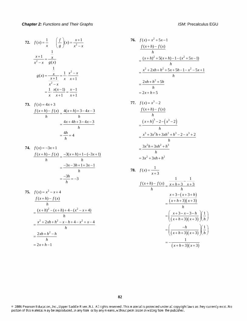
63. a. length = 24 2x− ; width = 24 2x− ; height = x
2( ) (24 2 )(24 2 ) (24 2 )V x x x x x x= − − = −
b. 2 2(3) 3(24 2(3)) 3(18)3(324) 972 cu.in.
V = − == =
c. 2 2(10) 10(24 2(10)) 10(4)10(16) 160 cu.in.
V = − == =
d. 21 (24 2 )y x x= −
120
1100
0 Use MAXIMUM.
0 12
1100
0 The volume is largest when 4x = inches.
64. a. Let amount of materialA = , length of the basex = , heighth = , and volumeV = . 2
21010V x h hx
= = ⇒ =
( ) ( )( )
( )
base side2
22
2
2
Total Area Area 4 Area
4104
40
40
A
x xh
x xx
xx
A x xx
= +
= +
⎛ ⎞= + ⎜ ⎟⎝ ⎠
= +
= +
b. ( ) 2 2401 1 1 40 41 ft1
A = + = + =
c. ( ) 2 2402 2 4 20 24 ft2
A = + = + =

ISM: Precalculus EGU Chapter 2: Functions and Their Graphs
101
d. 21
40y xx
= +
100
100
0
0 10
100
0 The amount of material is least when
2.71x = ft.
65. a. 21 16 80 6y x x= − + +
00
6
110
b. Use MAXIMUM. The maximum height
occurs when 2.5 seconds.t =
0 6
110
0 c. From the graph, the maximum height is 106
feet.
66. a. ( ) 217.28 100y s t t t= = − +
0 8
200
−25
b. Use the Maximum option on the CALC menu.
0 8
200
−25 The object reaches its maximum height after about 2.89 seconds.
c. From the graph in part (b), the maximum height is about 144.68 feet.
d. ( ) 216 100s t t t= − +
0 8
200
−25 On Earth, the object would reach a maximum height of 156.25 feet after 3.125 seconds. The maximum height is slightly higher than on Saturn.
67. ( ) 2 25000.3 21 251C x x xx
= + − +
a. 21
25000.3 21 251y x xx
= + − +
0 30
2500
−300
b. Use MINIMUM. The average cost is minimized when approximately 9.66 lawnmowers are produced per hour.
0 30
2500
−300
c. The minimum average cost is approximately $238.65.

Chapter 2: Functions and Their Graphs ISM: Precalculus EGU
102
68. a. ( ) 4 3 2.002 .039 .285 .766 .085C t t t t t= − + − + + Graph the function on a graphing utility and use the Maximum option from the CALC menu.
100
0
1
The concentration will be highest after about 2.16 hours.
b. Enter the function in Y1 and 0.5 in Y2. Graph the two equations in the same window and use the Intersect option from the CALC menu.
100
0
1
100
0
1
After taking the medication, the woman can feed her child within the first 0.71 hours (about 42 minutes) or after 4.47 hours (about 4hours 28 minutes) have elapsed.
69. (a), (b), (e)
c. 28000 0 28000Average rate25 0 25of change
1120 dollars/bicycle
−= =−
=
d. For each additional bicycle sold between 0 and 25, the total revenue increases by (an average of) $1120.
f. 64835 62360 2475Average rate223 190 33of change
75 dollars per bicycle
−= =−
=
g. For each additional bicycle sold between 190 and 223, the total revenue increases by (an average of) $75.
h. The average rate of change of revenue is decreasing as the number of bicycles increases.
70. (a), (b), (e)
c. 27750 24000Average rate25 0of change
3750 150 dollars/bicycle25
−=
−
= =
d. For each additional bicycle made between 0 and 25, the total production cost increases by (an average of) $150.
f. 46500 42750 3750Average rate223 190 33of change
113.64 dollars/bicycle
−= =
−
=
g. For each additional bicycle made between 190 and 223, the total production cost increases by (an average of) $113.64.
h. The average rate of change of cost is decreasing as the number of bicycles increases.
71. 2( )f x x=
a. Average rate of change of f from 0x = to 1x = :
( ) ( ) 2 21 0 1 0 1 11 0 1 1
f f− −= = =
−

ISM: Precalculus EGU Chapter 2: Functions and Their Graphs
103
b. Average rate of change of f from 0x = to 0.5x = :
( ) ( ) ( )2 20.5 0 0.5 0 0.25 0.50.5 0 0.5 0.5
f f− −= = =
−
c. Average rate of change of f from 0x = to 0.1x = :
( ) ( ) ( )2 20.1 0 0.1 0 0.01 0.10.1 0 0.1 0.1
f f− −= = =
−
d. Average rate of change of f from 0x = to 0.01x = :
( ) ( ) ( )2 20.01 0 0.01 00.01 0 0.01
0.0001 0.010.01
f f− −=
−
= =
e. Average rate of change of f from 0x = to 0.001x = :
( ) ( ) ( )2 20.001 0 0.001 00.001 0 0.001
0.000001 0.0010.001
f f− −=
−
= =
f. Graphing the secant lines:
g. The secant lines are beginning to look more and more like the tangent line to the graph of f at the point where x = 0.
h. The slopes of the secant lines are getting smaller and smaller. They seem to
be
approaching the number zero.
72. 2( )f x x=
a. Average rate of change of f from 1x = to 2x = :
( ) ( ) 2 22 1 2 1 3 32 1 1 1
f f− −= = =
− b. Average rate of change of f from 1x = to
1.5x = :
( ) ( ) ( )2 21.5 1 1.5 1 1.25 2.51.5 1 0.5 0.5
f f− −= = =
−
c. Average rate of change of f from 1x = to 1.1x = :
( ) ( ) ( )2 21.1 1 1.1 1 0.21 2.1
1.1 1 0.1 0.1f f− −
= = =−
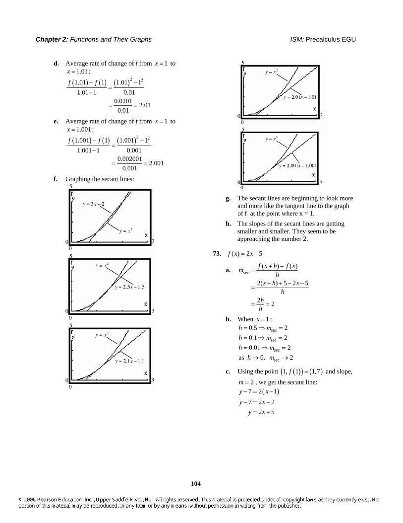
Chapter 2: Functions and Their Graphs ISM: Precalculus EGU
104
d. Average rate of change of f from 1x = to 1.01x = :
( ) ( ) ( )2 21.01 1 1.01 1
1.01 1 0.010.0201 2.010.01
f f− −=
−
= =
e. Average rate of change of f from 1x = to 1.001x = :
( ) ( ) ( )2 21.001 1 1.001 1
1.001 1 0.0010.002001 2.001
0.001
f f− −=
−
= =
f. Graphing the secant lines:
g. The secant lines are beginning to look more and more like the tangent line to the graph of f at the point where x = 1.
h. The slopes of the secant lines are getting smaller and smaller. They seem to be approaching the number 2.
73. ( ) 2 5f x x= +
a. sec( ) ( )
2( ) 5 2 5
2 2
f x h f xmh
x h xh
hh
+ −=
+ + − −=
= =
b. When 1x = : sec0.5 2h m= ⇒ = sec0.1 2h m= ⇒ =
sec0.01 2h m= ⇒ = secas 0, 2h m→ →
c. Using the point ( )( ) ( )1, 1 1,7f = and slope, 2m = , we get the secant line:
( )7 2 17 2 2
2 5
y xy x
y x
− = −
− = −= +

ISM: Precalculus EGU Chapter 2: Functions and Their Graphs
105
d. Graphing:
The graph and the secant line coincide.
74. ( ) 3 2f x x= − +
a. sec( ) ( )
3( ) 2 ( 3 2)
3 3
f x h f xmh
x h xh
hh
+ −=
− + + − − +=
−= = −
b. When x = 1, sec0.5 3h m= ⇒ = − sec0.1 3h m= ⇒ = −
sec0.01 3h m= ⇒ = − secas 0, 3h m→ → −
c. Using point ( )( ) ( )1, 1 1, 1f = − and slope = 3− , we get the secant line:
( ) ( )1 3 11 3 3
3 2
y xy x
y x
− − = − −
+ = − += − +
d. Graphing:
The graph and the secant line coincide.
75. 2( ) 2f x x x= +
a. sec
2 2
2 2 2
2
( ) ( )
( ) 2( ) ( 2 )
2 2 2 2
2 2
2 2
f x h f xmh
x h x h x xh
x xh h x h x xh
xh h hh
x h
+ −=
+ + + − +=
+ + + + − −=
+ +=
= + +
b. When x = 1, sec0.5 2 1 0.5 2 4.5h m= ⇒ = ⋅ + + =
sec0.1 2 1 0.1 2 4.1h m= ⇒ = ⋅ + + =
sec0.01 2 1 0.01 2 4.01h m= ⇒ = ⋅ + + =
secas 0, 2 1 0 2 4h m→ → ⋅ + + =
c. Using point ( )( ) ( )1, 1 1,3f = and slope = 4.01, we get the secant line:
( )3 4.01 13 4.01 4.01
4.01 1.01
y xy x
y x
− = −
− = −= −
d. Graphing:
76. 2( ) 2f x x x= +
a. sec( ) ( )f x h f xm
h+ −
=
2 2
2 2 2
2 2 2
2
2( ) ( ) (2 )
2( 2 ) 2
2 4 2 2
4 2
4 2 1
x h x h x xh
x xh h x h x xh
x xh h x h x xh
xh h hh
x h
+ + + − +=
+ + + + − −=
+ + + + − −=
+ +=
= + +

Chapter 2: Functions and Their Graphs ISM: Precalculus EGU
106
b. When x = 1, ( )sec0.5 4 1 2 0.5 1 6h m= ⇒ = ⋅ + + =
( )sec0.1 4 1 2 0.1 1 5.2h m= ⇒ = ⋅ + + =
( )sec0.01 4 1 2 0.01 1 5.02h m= ⇒ = ⋅ + + =
( )secas 0, 4 1 2 0 1 5h m→ → ⋅ + + =
c. Using point ( )( ) ( )1, 1 1,3f = and slope = 5.02, we get the secant line:
( )3 5.02 13 5.02 5.02
5.02 2.02
y xy x
y x
− = −
− = −= −
d. Graphing:
77. 2( ) 2 3 1f x x x= − +
a. sec( ) ( )f x h f xm
h+ −
=
( ) ( ) ( )2 2 2
2 2 2
2 2
2
2( 2 ) 3 3 1 2 3 1
2 4 2 3 3 1 2 3 1
2 3 1 2 3 1
4 2 3
4 2 3
x xh h x h x xh
x xh h x h x xh
x h x h x xh
xh h hh
x h
+ + − − + − + −=
+ + − − + − + −=
+ − + + − − +=
+ −=
= + −
b. When x = 1, ( )sec0.5 4 1 2 0.5 3 2h m= ⇒ = ⋅ + − = ( )sec0.1 4 1 2 0.1 3 1.2h m= ⇒ = ⋅ + − =
( )sec0.01 4 1 2 0.01 3 1.02h m= ⇒ = ⋅ + − = ( )secas 0, 4 1 2 0 3 1h m→ → ⋅ + − =
c. Using point ( )( ) ( )1, 1 1,0f = and slope = 1.02, we get the secant line:
( )0 1.02 11.02 1.02
y xy x
− = −
= −
d. Graphing:
78. 2( ) 3 2f x x x= − + −
a. sec( ) ( )f x h f xm
h+ −
=
( ) ( ) ( )2 2 2
2 2 2
2 2
2
( 2 ) 3 3 2 3 2
2 3 3 2 3 2
3 2 3 2
2 3
2 3
x xh h x h x xh
x xh h x h x xh
x h x h x xh
xh h hh
x h
− + + + + − + − +=
− − − + + − + − +=
− + + + − − − + −=
− − +=
= − − +
b. When x = 1, sec0.5 2 1 0.5 3 0.5h m= ⇒ = − ⋅ − + =
sec0.1 2 1 0.1 3 0.9h m= ⇒ = − ⋅ − + =
sec0.01 2 1 0.01 3 0.99h m= ⇒ = − ⋅ − + =
secas 0, 2 1 0 3 1h m→ → − ⋅ − + =
c. Using point ( )( ) ( )1, 1 1,0f = and slope = 0.99, we get the secant line:
( )0 0.99 10.99 0.99
y xy x
− = −
= −
d. Graphing:

ISM: Precalculus EGU Chapter 2: Functions and Their Graphs
107
79. 1( )f xx
=
a.
( )( )
( )
( )
( )
sec
1 1( ) ( )
1
1
1
x h xf x h f xmh h
x x hx h x x x h
h hx h x
hhx h x
x h x
⎛ ⎞−⎜ ⎟++ − ⎝ ⎠= =
− +⎛ ⎞⎜ ⎟+ ⎛ ⎞− − ⎛ ⎞⎝ ⎠= = ⎜ ⎟⎜ ⎟+ ⎝ ⎠⎝ ⎠⎛ ⎞− ⎛ ⎞= ⎜ ⎟⎜ ⎟+ ⎝ ⎠⎝ ⎠
= −+
b. When x = 1,
0.5h = ⇒( )( )sec
11 0.5 11 0.667
1.5
m = −+
= − ≈ −
0.1h = ⇒( )( )sec
11 0.1 11 0.909
1.1
m = −+
= − ≈ −
0.01h = ⇒( )( )sec
11 0.01 11 0.990
1.01
m = −+
= − ≈ −
as 0, h →( )( )sec
1 1 111 0 1
m → − = − = −+
c. Using point ( )( ) ( )1, 1 1,1f = and slope = 0.990− , we get the secant line:
( )1 0.99 11 0.99 0.99
0.99 1.99
y xy x
y x
− = − −
− = − += − +
d. Graphing:
80. 21( )f xx
=
a.
( )
sec
2 2
( ) ( )
1 1
f x h f xmh
xx hh
+ −=
⎛ ⎞⎜ ⎟−⎜ ⎟+⎝ ⎠=
( )( )
( )( )
( )
( )
22
2 2
2 2 2
2 2
2
2 2
2 2
2 1
2 1
2
x x h
x h xh
x x xh hhx h x
xh hhx h x
x hx h x
⎛ ⎞− +⎜ ⎟⎜ ⎟+⎝ ⎠=
⎛ ⎞− + + ⎛ ⎞⎜ ⎟= ⎜ ⎟⎜ ⎟⎝ ⎠+⎝ ⎠⎛ ⎞− − ⎛ ⎞⎜ ⎟= ⎜ ⎟⎜ ⎟⎝ ⎠+⎝ ⎠
− −=+
b. When x = 1,
( )sec 2 2
2 1 0.50.5 1.1111 0.5 1
h m − ⋅ −= ⇒ = ≈ −+
( )sec 2 2
2 1 0.10.1 1.7361 0.1 1
h m − ⋅ −= ⇒ = ≈ −+
( )sec 2 2
2 1 0.010.01 1.9701 0.01 1
h m − ⋅ −= ⇒ = ≈ −+
( )sec 2 2
2 1 0as 0, 21 0 1
h m − ⋅ −→ → = −+
c. Using point ( )( ) ( )1, 1 1,1f = and slope = 1.970− , we get the secant line:
( )1 1.970 11 1.97 1.97
1.97 2.97
y xy x
y x
− = − −
− = − += − +
d. Graphing:

Chapter 2: Functions and Their Graphs ISM: Precalculus EGU
108
81. Answers will vary. One possibility follows:
−2 4
−5
y
2
(0, 3)−
(3, 0)
(2, 6)−
( 1, 2)− −
82. Answers will vary. See solution to Problem 81 for one possibility.
83. A function that is increasing on an interval can have at most one x-intercept on the interval. The graph of f could not "turn" and cross it again or it would start to decrease.
84. An increasing function is a function whose graph goes up as you read from left to right.
5
−5
y
−3 3
A decreasing function is a function whose graph goes down as you read from left to right.
5
−5
y
−3 3
85. To be an even function we need ( ) ( )f x f x− = and to be an odd function we need
( ) ( )f x f x− = − . In order for a function be both
even and odd, we would need ( ) ( )f x f x= − .
This is only possible if ( ) 0f x = .
86. The graph of 5y = is a horizontal line.
The local maximum is 5y = and it occurs at each x-value in the interval.
Section 2.4
1. From the equation 2 3y x= − , we see that the y-intercept is 3− . Thus, the point ( )0, 3− is on the graph. We can obtain a second point by choosing a value for x and finding the corresponding value for y. Let 2x = , then ( )2 2 3 1y = − = . Thus, the point
( )2,1 is also on the graph. Plotting the two points and connecting with a line yields the graph below.
y
x
5
5−5−2
(0, 3)−
(2, 1)
2. 2 1
2 1
3 5 2 21 2 3 3
y ym
x x− − −= = = =− − − −

ISM: Precalculus EGU Chapter 2: Functions and Their Graphs
109
3. We can use the point-slope form of a line to obtain the equation.
( )( )( )
( )
1 1
5 3 1
5 3 15 3 3
3 2
y y m x x
y x
y xy x
y x
− = −
− = − − −
− = − +
− = − −= − +
4. 6 900 15 285021 900 2850
21 37501250
7
x xx
x
x
− = − +− =
=
=
5. slope; y-intercept
6. scatter diagram
7. y kx=
8. True
9. True
10. True
11. ( ) 2 3f x x= + Slope = average rate of change = 2; y-intercept = 3
12. ( ) 5 4g x x= − Slope = average rate of change = 5; y-intercept = –4
13. ( ) 3 4h x x= − + Slope = average rate of change = –3; y-intercept = 4
14. p x( ) = −x + 6 Slope = average rate of change = –1; y-intercept = 6

Chapter 2: Functions and Their Graphs ISM: Precalculus EGU
110
15. ( ) 1 34
f x x= −
1Slope average rate of change = 4
= ;
y-intercept = –3
16. ( ) 2 43
h x x= − +
2Slope average rate of change = 3
= − ;
y-intercept = 4
17. ( ) 4F x = Slope = average rate of change = 0; y-intercept = 4
18. ( ) 2G x = − Slope = average rate of change = 0; y-intercept = –2
19. Linear, 0m >
20. Nonlinear
21. Linear, 0m <
22. No relation
23. Nonlinear
24. Nonlinear
25. a.
10
20
00
b. Answers will vary. We select (3, 4) and (9, 16). The slope of the line containing these points is:
16 4 12 29 3 6
m −= = =−
The equation of the line is: 1 1( )4 2( 3)4 2 6
2 2
y y m x xy xy x
y x
− = −− = −− = −
= −
c.
10
20
00

ISM: Precalculus EGU Chapter 2: Functions and Their Graphs
111
d. Using the LINear REGresssion program, the line of best fit is:
2.0357 2.3571y x= −
e.
10
20
00
26. a.
150
12
–2 b. Selection of points will vary. We select
(3, 0) and (13, 11). The slope of the line containing these points is:
11 0 11 1.113 3 10
m −= = =−
The equation of the line is: 1 1( )0 1.1( 3)0 1.1 3.3
1.1 3.3
y y m x xy xy x
y x
− = −− = −− = −
= −
c.
150
12
–2 d. Using the LINear REGression program, the
line of best fit is: 1.1286 3.8619y x= −
e.
150
12
–2
27. a.
3
6
–3
–6 b. Answers will vary. We select (–2,–4) and
(1, 4). The slope of the line containing these points is:
4 ( 4) 81 ( 2) 3
m − −= =
− −
The equation of the line is: 1 1( )
8( 4) ( ( 2))38 1643 38 43 3
y y m x x
y x
y x
y x
− = −
− − = − −
+ = +
= +
c.
3
6
–3
–6 d. Using the LINear REGresssion program,
the line of best fit is: 2.2 1.2y x= +
e.
3
6
–3
–6 28. a.
3–3
8
–2

Chapter 2: Functions and Their Graphs ISM: Precalculus EGU
112
b. Selection of points will vary. We select (–2, 7) and (1, 2). The slope of the line containing these points is:
52 7 51 ( 2) 3 3
m −−= = = −− −
The equation of the line is: 1 1
535 103 35 113 3
( )
7 ( ( 2))
7
y y m x x
y x
y x
y x
− = −
− = − − −
− = − −
= − +
c.
−8
−5 5
8
d. Using the LINear REGression program, the
line of best fit is: 1.8 3.6y x= − +
e.
3–3
8
–2 29. a.
0
160
–2590
b. Answers will vary. We select (–20,100) and (–15,118). The slope of the line containing these points is:
( )118 100 18 3.6
515 20m −= = =
− − −
The equation of the line is:
( )1 1( )
100 3.6( 20 )100 3.6 72
3.6 172
y y m x xy xy x
y x
− = −
− = − −
− = += +
c.
0
160
–2590
d. Using the LINear REGresssion program, the line of best fit is:
3.8613 180.2920y x= +
e.
0
160
–2590
30. a.
0–35
20
0 b. Selection of points will vary. We select
(–30, 10) and (–14, 18). The slope of the line containing these points is:
( )18 10 8 0.5
1614 30m −= = =
− − −
The equation of the line is:
( )1 1( )
10 0.5( 30 )10 0.5 15
0.5 25
y y m x xy xy x
y x
− = −
− = − −
− = += +
c.
00−40
25
d. Using the LINear REGression program, the
line of best fit is: 0.4421 23.4559y x= +

ISM: Precalculus EGU Chapter 2: Functions and Their Graphs
113
e.
00−40
25
31. a. ( )( ) ( )
0.25 35
40 0.25 40 35 45
C x x
C
= +
= + =
The moving truck will cost $45.00 if you drive 40 miles.
b. 80 0.25 3545 0.25
180
xx
x
= +==
If the cost of the truck is $80.00, you drove for 180 miles.
c. 100 0.25 3565 0.25
260
xx
x
= +==
To keep the cost below $100, you must drive less than 260 miles.
32. a. ( )( ) ( )
0.38 5
50 0.38 50 5 24
C x x
C
= +
= + =
If you talk for 50 minutes, the cost will be $24.00.
b. 29.32 0.38 524.32 0.38
64
xx
x
= +==
If the monthly bill is $29.32, you would have used the phone for 64 minutes.
c. 60 0.38 555 0.38
144.74
xx
x
= +=≈
To stay within budget, you can talk for no more than 144 minutes.
33. a. ( )( ) ( )
19.25 585.72
10 19.25 10 585.72 778.22
B t t
B
= +
= + =
The average monthly benefit in 2000 was $778.22.
b. 893.72 19.25 585.72308 19.2516
tt
t
= +==
The average monthly benefit will be $893.72 in 2006.
c. 1000 19.25 585.72414.28 19.2521.52
tt
t
= +=≈
The average monthly benefit will exceed $1000 in 2012.
34. a. ( )( ) ( )
26 411
10 26 10 411 671
H t t
H
= +
= + =
The total private health expenditures in 2000 was $671 billion.
b. 879 26 411468 2618
tt
t
= +==
Total private health expenditures will be $879 billion in 2008.
c. 1000 26 411589 26
22.65
tt
t
= +==
Total private health expenditures will exceed $1 trillion in 2013.
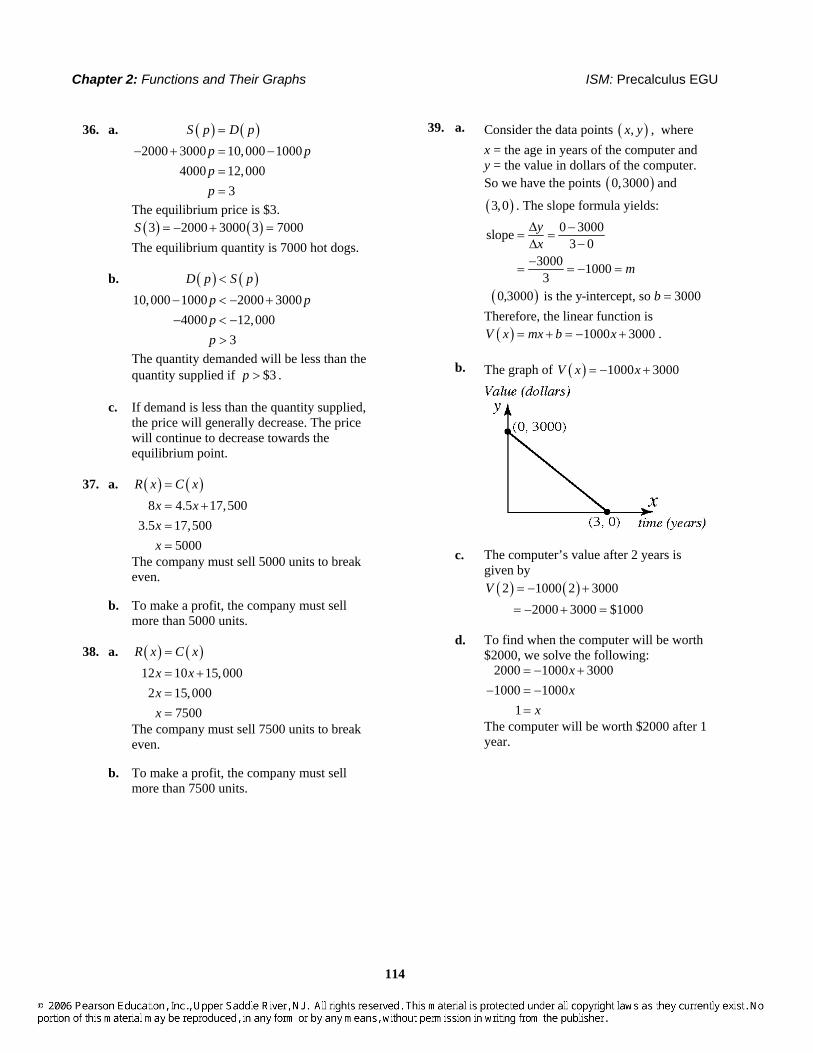
35. a. ( ) ( )200 50 1000 25
75 120016
S p D pp ppp
=
− + = −==
The equilibrium price is $16. ( ) ( )16 200 50 16 600S = − + =
The equilibrium quantity is 600 T-shirts.
b. ( ) ( )1000 25 200 50
75 120016
D p S pp ppp
>
− > − +− > −
<
The quantity demanded will exceed the quantity supplied if 0 $16p< < .
c. If demand is higher than supply, generally the price will increase. The price will continue to increase towards the equilibrium point.
Chapter 2: Functions and Their Graphs ISM: Precalculus EGU
114
36. a. ( ) ( )2000 3000 10,000 1000
4000 12,0003
S p D pp ppp
=
− + = −==
The equilibrium price is $3. ( ) ( )3 2000 3000 3 7000S = − + =
The equilibrium quantity is 7000 hot dogs.
b. ( ) ( )10,000 1000 2000 3000
4000 12,0003
D p S pp ppp
<
− < − +− < −
>
The quantity demanded will be less than the quantity supplied if $3p > .
c. If demand is less than the quantity supplied, the price will generally decrease. The price will continue to decrease towards the equilibrium point.
37. a. ( ) ( )8 4.5 17,500
3.5 17,5005000
R x C xx xxx
=
= +==
The company must sell 5000 units to break even.
b. To make a profit, the company must sell more than 5000 units.
38. a. ( ) ( )12 10 15,000
2 15,0007500
R x C xx xxx
=
= +==
The company must sell 7500 units to break even.
b. To make a profit, the company must sell more than 7500 units.
39. a. Consider the data points ( ),x y , where x = the age in years of the computer and y = the value in dollars of the computer. So we have the points ( )0,3000 and
( )3,0 . The slope formula yields: 0 3000slope
3 03000 10003
yx
m
Δ −= =Δ −−= = − =
( )0,3000 is the y-intercept, so 3000b = Therefore, the linear function is
( ) 1000 3000V x mx b x= + = − + .
b. The graph of ( ) 1000 3000V x x= − +
c. The computer’s value after 2 years is given by
( ) ( )2 1000 2 3000 2000 3000 $1000
V = − +
= − + =
d. To find when the computer will be worth $2000, we solve the following:
2000 1000 30001000 1000
1
xx
x
= − +− = −
=
The computer will be worth $2000 after 1 year.

ISM: Precalculus EGU Chapter 2: Functions and Their Graphs
115
40. a. Consider the data points ( ),x y , where x = the age in years of the machine and y = the value in dollars of the machine. So we have the points ( )0,120000 and
( )10,0 . The slope formula yields: 0 120000 120000slope
10 0 1012000
yx
m
Δ − −= = =Δ −
= − =
( )0,120000 is the y-intercept, so 120000b = . Therefore, the linear function
is ( ) 12000 120000V x mx b x= + = − + .
b. The graph of ( ) 12000 120000V x x= − +
c. The machine’s value after 4 years is given by
( ) ( )4 12000 4 120000 48000 120000
$72000
V = − +
= − +=
d. To find when the machine will be worth $60,000, we solve the following:
60,000 12,000 120,00060,000 12,000
5
xx
x
= − +− = −
=
The machine will be worth $60,000 after 5 years.
41. a. Let x = the number of bicycles manufactured. We can use the cost function ( )C x mx b= + , with m = 90 and
b = 1800. Therefore ( ) 90 1800C x x= +
b. The graph of ( ) 90 1800C x x= +
c. The cost of manufacturing 14 bicycles is given by ( ) ( )14 90 14 1800 $3060C = + = .
d. To determine the number of bicycles, we solve the following: 3780 90 18001980 90
22
xx
x
= +==
The company can manufacture 22 bicycles for $3780.
42. a. The new daily fixed cost is 1001800 $180520
+ = .
b. Let x = the number of bicycles manufactured. We can use the cost function ( )C x mx b= + , with m = 90 and
b = 1805. Therefore ( ) 90 1805C x x= + .
c. The graph of ( ) 90 1805C x x= +
d. The cost of manufacturing 14 bicycles is given by ( ) ( )14 90 14 1805 $3065C = + = .

Chapter 2: Functions and Their Graphs ISM: Precalculus EGU
116
e. To determine the number of bicycles, we solve the following: 3780 90 18051975 90
21.94
xx
x
= +=≈
The company can manufacture 21 complete bicycles for $3780.
43. a. Let x = number of miles driven and C = cost in dollars to rent a truck for one day. Since the fixed daily charge is $29 and the variable mileage charge is $0.07 per mile, we have
( ) 0.07 29C x x= + .
b. ( ) ( )( ) ( )110 0.07 110 29 36.70
230 0.07 230 29 45.10
C
C
= + =
= + =
It will cost $36.70 for one day if the truck is driven 110 miles, and it will cost $45.10 if the truck is driven 230 miles.
44. a. Let x = number of minutes talking and C = cost in dollars. Since the fixed charge is $5 and the variable time charge is $0.05 per minute, we have
( ) 0.05 5C x x= + .
b. ( ) ( )( ) ( )105 0.05 105 5 $10.25
180 0.05 180 5 $14.00
C
C
= + =
= + =
The plan will cost $10.25 if you talk for 105 minutes, and it will cost $14.00 if you talk for 180 minutes.
45. Let p = the monthly payment and B = the amount borrowed. Consider the ordered pair ( ),B p . We can use the points ( )0,0 and
( )1000,6.49 . Now compute the slope:
6.49 0 6.49slope 0.006491000 0 1000
yx
Δ −= = = =
Δ −
Therefore we have the linear function ( ) 0.00649 0 0.00649p B B B= + = .
If 145000B = , then ( )( )0.00649 145000 $941.05p = = .
46. Let p = the monthly payment and B = the amount borrowed. Consider the ordered pair ( ),B p . We can use the points ( )0,0 and
( )1000,8.99 . Now compute the slope:
8.99 0 8.99slope 0.008991000 0 1000
yx
Δ −= = = =
Δ −
Therefore we have the linear function ( ) 0.00899 0 0.00899p B B B= + = .
If 175000B = , then ( )( )0.00899 175000 $1573.25p = = .
47. Let R = the revenue and g = the number of gallons of gasoline sold. Consider the ordered pair ( ),g R . We can use the points ( )0,0 and
( )12, 23.40 . Now compute the slope:
23.40 0 23.40slope 1.9512 0 12
yx
Δ −= = = =
Δ −
Therefore we have the linear function ( ) 1.95 0 1.95R g g g= + = .
If 10.5g = , then ( )( )1.95 10.5 $20.48R = = .
48. Let C = the cost and A = the number of gallons almonds purchased. Consider the ordered pair ( ),A C . We can use the points ( )0,0 and
( )5, 23.75 . Now compute the slope:
23.75 0 23.75slope 4.755 0 5
yx
Δ −= = = =
Δ −
Therefore we have the linear function ( ) 4.75 0 4.75C A A A= + = .
If 3.5A = , then ( )( )4.75 3.5 $16.63C = = .
49. W kS= ( )1.875 15
0.125kk
=
=
For 40 gallons of sand: ( )0.125 40 5W = = gallons of water.
50. v kt= ( )
( )( )
64 2 32in 3 seconds
32 3 96 feet per second
k k
v
= ⇒ =
= =

ISM: Precalculus EGU Chapter 2: Functions and Their Graphs
117
51. a.
19,000 30,00017,500
28,000
b.
( ) 0.9241 479.6584C I I= +
c. The slope indicates that for each $1 increase in per capita disposable income, there is an increase of $0.92 in per capita consumption.
d. ( ) ( )28,750 0.9241 28,750 479.658427,047.53
C = +
=When disposable income is $28,750, the per capita consumption is about $27,048.
e. 26,900 0.9241 479.658426,420.3416 0.9241
28,590.35
II
I
= +==
When comsumption is $26,500, the per capita disposable income is about $28,590.
52. a.
b. Using the LINear REGression program, the line of best fit is:
( ) 0.3734 7.3268C H H= +
c. For each 1 inch increase in height, the circumference increases by 0.3734 inch.
d. ( ) ( )26 0.3734 26 7.3268C = + 17.035≈ inches
e. To find the height, we solve the following equation:
17.4 0.3734 7.326810.0732 0.3734
26.98
HH
H
= +=≈
A child with a head circumference of 17.4 inches would have a height of about 26.98 inches.
53. a.
b. Using the LINear REGression program, the line of best fit is:
( ) 0.0261 7.8738L G G= +
c. For each 1 day increase in Gestation period, the life expectancy increases by 0.0261 years (about 9.5 days).
d. ( ) ( )89 0.0261 89 7.8738L = + 10.2≈ years
54. a. (Data used in graphs is in thousands.)
800
220
30
b. 2.9814 0.0761072L I= − (data in thousands) or 2.9814 76.1072L I= −
c.
80
220
030
d. As annual income increases by $1, the loan amount increases by $2.98.

Chapter 2: Functions and Their Graphs ISM: Precalculus EGU
118
e. 2.9814(42) 0.0761072L = − 125.143= A person with an annual income of $42,000 would qualify for a loan of about $125,143.
55. a. The relation is not a function because 23 is paired with both 56 and 53.
b.
3218
65
40
c. Using the LINear REGression program, the line of best fit is:
1.3355 86.1974D p= − +
d. As the price of the jeans increases by $1, the demand for the jeans decreases by 1.3355 pairs per day.
e. ( ) 1.3355 86.1974D p p= − +
f. Domain: { }0 64p p< < Note that the p-intercept is roughly 64.54 and that the number of pairs cannot be negative.
g. ( ) ( )28 1.3355 28 86.1974 48.8034D = − +
≈ Demand is about 49 pairs.
56. a. The relation is not a function because 24 is paired with both 343 and 341.
b.
3018
355
330
c. Using the LINear REGression program, the line of best fit is:
2.0667 292.8869S A= +
d. As the advertising expenditure increases by $1000, the sales increase by $2066.70.
e. ( ) 2.0667 292.8869S A A= +
f. Domain: { }0A A ≥
g. ( ) ( )25 2.0667 25 292.8869 344.5544S = +
≈
Sales are about $344,554.
57. The data do not follow a linear pattern so it would not make sense to find the line of best fit.
30
−10
60
50
58. The data do not follow a linear pattern so it would not make sense to find the line of best fit.
−1
−10
16
70
59. A linear function is odd if the y-intercept is 0. That is, if the line passes through the origin. A linear function can be even if the slope is 0.
60. Using the ordered pairs ( )1,5 and ( )3,8 , the line
of best fit is 3 72 2
y x= + .
The correlation coefficient is 1r = . This makes sense because two points completely determine a line.
61. A correlation coefficient of 0 implies that there is no linear relationship between the data.
62. If the student’s average in the class is directly proportional to the amount of time the student studies, the relationship between the average and time studying would be linear. That is, we could express the relationship as A kT= where T is the time spent studying and A is the student’s average.

ISM: Precalculus EGU Chapter 2: Functions and Their Graphs
119
Section 2.5
1. y = x
2. y =1x
3. y = x 3 − 8 y-intercept: Let 0x = , then ( )30 8 8y = − = − .
x-intercept: Let 0y = , then 3
3
0 8
82
x
xx
= −
==
The intercepts are ( )0, 8− and ( )2,0 .
4. less
5. piecewise defined
6. True
7. False; the cube root function is odd and increasing on the interval ( ),−∞ ∞ .
8. False; the domain and range of the reciprocal function are both the set of real numbers except for 0.
9. C
10. A
11. E
12. G
13. B
14. D
15. F
16. H
17. ( )f x x=
18. ( ) 2f x x=

Chapter 2: Functions and Their Graphs ISM: Precalculus EGU
120
19. ( ) 3f x x=
20. ( )f x x=
21. ( ) 1f xx
=
22. ( )f x x=
23. 3( )f x x=
24. ( ) 3f x =
25. a. 2( 2) ( 2) 4f − = − =
b. (0) 2f =
c. (2) 2(2) 1 5f = + =
26. a. 3( 1) ( 1) 1f − = − = −
b. (0) 3(0) 2 2f = + =
c. (1) 3(1) 2 5f = + =
27. a. (1.2) int(2(1.2)) int(2.4) 2f = = =
b. (1.6) int(2(1.6)) int(3.2) 3f = = =
c. ( 1.8) int(2( 1.8)) int( 3.6) 4f − = − = − = −

ISM: Precalculus EGU Chapter 2: Functions and Their Graphs
121
28. a. 1.2(1.2) int int(0.6) 02
f ⎛ ⎞= = =⎜ ⎟⎝ ⎠
b. 1.6(1.6) int int(0.8) 02
f ⎛ ⎞= = =⎜ ⎟⎝ ⎠
c. 1.8( 1.8) int int( 0.9) 12
f −⎛ ⎞− = = − = −⎜ ⎟⎝ ⎠
29. 2 if 0
( )1 if 0
x xf x
x≠⎧
= ⎨ =⎩
a. Domain: { } is any real numberx x
b. x-intercept: none y-intercept: (0,1)
c. Graph:
d. Range: { }0y y ≠
30. 3 if 0
( )4 if 0x x
f xx
≠⎧= ⎨ =⎩
a. Domain: { } is any real numberx x
b. x-intercept: none y-intercept: (0, 4)
c. Graph:
5
−5
y
5−5
(0, 4)(1, 3)
(−1, −3)
d. Range: { }0y y ≠
31. 2 3 if 1
( )3 2 if 1
x xf x
x x− + <⎧
= ⎨ − ≥⎩
a. Domain: { } is any real numberx x
b. x-intercept: none y-intercept: (0,3)
c. Graph:
d. Range: { }1y y ≥
32. 3 if 2
( )2 3 if 2
x xf x
x x+ < −⎧
= ⎨− − ≥ −⎩
a. Domain: { } is any real numberx x
b. x-intercepts: (–3, 0), (–1.5, 0) y-intercept: (0, –3)
c. Graph:
d. Range: { }1y y ≤
33. 3 if 2 1
( ) 5 if 12 if 1
x xf x x
x x
+ − ≤ <⎧⎪= =⎨⎪− + >⎩
a. Domain: { }2x x ≥ −
b. x-intercept: (2, 0) y-intercept: (0, 3)

Chapter 2: Functions and Their Graphs ISM: Precalculus EGU
122
c. Graph:
d. Range: { }4 and 5y y y< =
34. 2 5 if 3 0
( ) 3 if 05 if 0
x xf x x
x x
+ − ≤ <⎧⎪= − =⎨⎪− >⎩
a. Domain: { }3x x ≥ −
b. x-intercept: (–2.5, 0) y-intercept: (0, –3)
c. Graph:
d. Range: { }5y y <
35. 2
1 if 0( )
if 0
x xf x
x x
+ <⎧⎪= ⎨≥⎪⎩
a. Domain: { } is any real numberx x
b. x-intercepts: (–1,0), (0,0) y-intercept: (0,0)
c. Graph:
d. Range: { } is any real numbery y
36. 3
1 if 0( )
if 0
xxf xx x
⎧ <⎪= ⎨⎪ ≥⎩
a. Domain: { }is any real numberx x
b. x-intercept: (0,0) y-intercept: (0,0)
c. Graph:
d. Range: { }is any real numbery y
37. 3
if 2 0( ) 1 if 0
if 0
x xf x x
x x
⎧ − ≤ <⎪
= =⎨⎪ >⎩
a. Domain: { }2x x ≥ −
b. x-intercept: none y-intercept: (0, 1)
c. Graph:
d. Range: { }0y y >
38. 3 if 3 0
( ) 3 if 0
if 0
x xf x x
x x
⎧ + − ≤ <⎪
= =⎨⎪ >⎩
a. Domain: { }3x x ≥ −
b. x-intercept: (–3, 0) y-intercept: (0, 3)

ISM: Precalculus EGU Chapter 2: Functions and Their Graphs
123
c. Graph:
d. Range: { }0y y ≥
39. ( ) 2int( )f x x=
a. Domain: { } is any real numberx x
b. x-intercepts: all ordered pairs ( ,0) when 0 1.x x≤ < y-intercept: (0,0)
c. Graph:
d. Range: { } is an even integery y
40. ( ) int(2 )f x x=
a. Domain: { } is any real numberx x
b. x-intercepts: all ordered pairs
1( ,0) when 0 .2
x x≤ <
y-intercept: (0,0)
c. Graph:
d. Range: { } is an integery y
41. if 1 0
( ) 1 if 0 22
x xf x
x x
− − ≤ ≤⎧⎪= ⎨
< ≤⎪⎩
42. if 1 0
( )1 if 0 2x x
f xx
− ≤ ≤⎧= ⎨ < ≤⎩
43. if 0
( )2 if 0 2
x xf x
x x− ≤⎧
= ⎨− + < ≤⎩
44. 2 2 if 1 0
( ) if >0
x xf x
x x+ − ≤ ≤⎧
= ⎨⎩
45. 35 if 0 3000.40 85 if 300
xC
x x< ≤⎧
= ⎨ − >⎩
a. ( )200 $35.00C =
b. ( ) ( )365 0.40 365 85 $61.00C = − =
c. ( ) ( )301 0.40 301 85 $35.40C = − =
46. ( ) ( )3 if 0 35int 1 1 if 3 950 if 9 24
xF x x x
x
< ≤⎧⎪= + + < <⎨⎪ ≤ ≤⎩
a. ( )2 3F = Parking for 2 hours costs $3.
b. ( ) ( )7 5int 7 1 1 41F = + + = Parking for 7 hours costs $41.
c. ( )15 50F = Parking for 15 hours costs $50.
d. 1 hr24 min 0.4 hr60 min
⋅ =
( ) ( ) ( )8.4 5int 8.4 1 1 5 9 1 46F = + + = + = Parking for 8 hours and 24 minutes costs $46.

Chapter 2: Functions and Their Graphs ISM: Precalculus EGU
124
47. a. Charge for 50 therms: 9.45 0.6338(50) 0.36375(50)$59.33
C = + +=
b. Charge for 500 therms: 9.45 0.36375(50) 0.11445(450)
0.6338(500)$396.04
C = + ++
=
c. For 0 50x≤ ≤ : 9.45 0.36375 0.63389.45 0.99755
C x xx
= + += +
For 50x > :
( ) ( )9.45 0.36375 50 0.11445 50 0.6338
9.45 18.1875 0.11445 5.7225 0.6338
21.915 0.74825
C xx
xx
x
= + + −
+= + + −
+= +
The monthly charge function:
9.45 0.99755 for 0 5021.915 0.74825 for 50
x xC
x x+ ≤ ≤⎧
= ⎨ + >⎩
d. Graphing:
48. a. Charge for 40 therms: 6.45 0.2012(20) 0.1117(20)
0.7268(40)$41.78
C = + ++
=
b. Charge for 202 therms: 6.45 0.2012(20) 0.1117(30)
0.0374(152) 0.7268(202)$166.32
C = + ++ +
=
c. For 0 20x≤ ≤ : 6.45 0.2012 0.72686.45 0.928
C x xx
= + += +
For 20 50x< ≤ :
( ) ( )6.45 0.2012 20 0.1117 20 0.7268
6.45 4.024 0.1117 2.234 0.72688.24 0.8385
C xx
xx
x
= + + −
+= + + −
+= +
For 50x > :
( ) ( )( )
6.45 0.2012 20 0.1117 30
0.0374 50 0.72686.45 4.024 3.351 0.0374 1.87
0.726811.955 0.7642
C
x xx
xx
= + +
+ − +
= + + + −+
= +
The monthly charge function:
( )0.928 if 0 200.8385 8.24 if 20 500.7642 11.955 if 50
x xC x x x
x x
≤ ≤⎧⎪= + < ≤⎨⎪ + >⎩
d. Graphing:
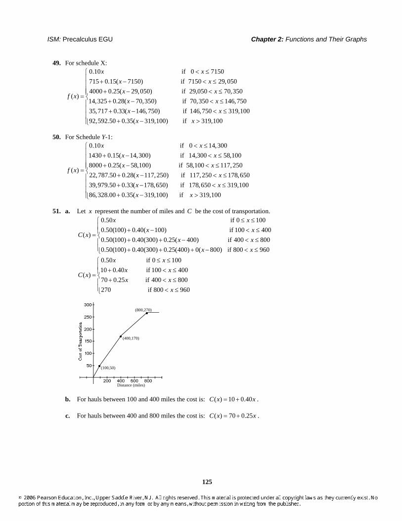
ISM: Precalculus EGU Chapter 2: Functions and Their Graphs
125
49. For schedule X: 0.10 if 0 7150715 0.15( 7150) if 7150 29,0504000 0.25( 29,050) if 29,050 70,350
( )14,325 0.28( 70,350) if 70,350 146,7
x xx x
x xf x
x x
< ≤+ − < ≤
+ − < ≤=
+ − < ≤ 5035,717 0.33( 146,750) if 146,750 319,10092,592.50 0.35( 319,100) if 319,100
x xx x
⎧⎪⎪⎪⎪⎨⎪⎪ + − < ≤⎪
+ − >⎪⎩
50. For Schedule Y-1: 0.10 if 0 14,3001430 0.15( 14,300) if 14,300 58,1008000 0.25( 58,100) if 58,100 117, 250
( )22,787.50 0.28( 117,250) if 117,250 178,6
x xx xx x
f xx x
< ≤+ − < ≤+ − < ≤
=+ − < ≤ 50
39,979.50 0.33( 178,650) if 178,650 319,10086,328.00 0.35( 319,100) if 319,100
x xx x
⎧⎪⎪⎪⎪⎨⎪⎪ + − < ≤⎪
+ − >⎪⎩
51. a. Let x represent the number of miles and C be the cost of transportation. 0.50 if 0 1000.50(100) 0.40( 100) if 100 400
( )0.50(100) 0.40(300) 0.25( 400) if 400 8000.50(100) 0.40(300) 0.25(400) 0( 800) if 800 960
x xx x
C xx x
x x
≤ ≤⎧⎪ + − < ≤⎪= ⎨ + + − < ≤⎪⎪ + + + − < ≤⎩
0.50 if 0 10010 0.40 if 100 400
( )70 0.25 if 400 800270 if 800 960
x xx x
C xx x
x
≤ ≤⎧⎪ + < ≤⎪= ⎨ + < ≤⎪⎪ < ≤⎩
Distance (miles)
(100,50)
(400,170)
(800,270)
b. For hauls between 100 and 400 miles the cost is: ( ) 10 0.40C x x= + .
c. For hauls between 400 and 800 miles the cost is: ( ) 70 0.25C x x= + .

Chapter 2: Functions and Their Graphs ISM: Precalculus EGU
126
52. Let x = number of days car is used. The cost of renting is given by
( )
95 if 7119 if 7 8143 if 8 9167 if 9 10190 if 10 14
xx
C x xxx
=⎧⎪ < ≤⎪⎪= < ≤⎨⎪ < ≤⎪
< ≤⎪⎩
x
C
95 119 143 167 190
7 8 9 10 11 12 13 14
53. Let x = the amount of the bill in dollars. The minimum payment due is given by
( )
if 1010 if 10 50030 if 500 100050 if 1000 150070 if 1500
x xx
f x xxx
<⎧⎪ ≤ <⎪⎪= ≤ <⎨⎪ ≤ <⎪
≤⎪⎩
54. Let x = the balance of the bill in dollars. The monthly interest charge is given by
( ) ( )0.015 if 100015 0.01 1000 if 1000
0.015 if 1000
5 0.01 if 1000
x xg x
x x
x xx x
≤⎧⎪= ⎨ + − <⎪⎩≤⎧
= ⎨ + <⎩
55. a. 10W C= °
b. (10.45 10 5 5)(33 10)3322.04
3.98
W
C
+ − −= −
≈ °
c. (10.45 10 15 15)(33 10)3322.04
2.67
W
C
+ − −= −
≈ − °
d. 33 1.5958(33 10) 3.7W C= − − = − °
e. When 0 1.79v≤ < , the wind speed is so small that there is no effect on the temperature.
f. For each drop of 1˚ in temperature, the wind chill factor drops approximately 1.6˚C. When the wind speed exceeds 20, there is a constant drop in temperature. That is, the windchill depends only on the temperature.
56. a. 10W C= − °
b. ( ) ( )( )10.45 10 5 5 33 10
3322.04
21.26
W
C
+ − − −= −
≈ − °
c. ( ) ( )( )10.45 10 15 15 33 10
3322.04
33.68
W
C
+ − − −= −
≈ − °
d. ( )( )33 1.5958 33 10 35.62W C= − − − = − °

ISM: Precalculus EGU Chapter 2: Functions and Their Graphs
127
57. Each graph is that of 2y x= , but shifted vertically.
If 2 , 0y x k k= + > , the shift is up k units; if
2 , 0y x k k= + < , the shift is down k units.
The graph of 2 4y x= − is the same as the graph
of 2y x= , but shifted down 4 units. The graph
of 2 5y x= + is the graph of 2y x= , but shifted up 5 units.
58. Each graph is that of 2y x= , but shifted horizontally.
If 2( ) , 0y x k k= − > , the shift is to the right k
units; if 2( ) , 0y x k k= − < , the shift is to the
left k units. The graph of 2( 4)y x= + is the
same as the graph of 2y x= , but shifted to the
left 4 units. The graph of 2( 5)y x= − is the
graph of 2y x= , but shifted to the right 5 units.
59. Each graph is that of y x= , but either compressed or stretched vertically.
If y k x= and 1k > , the graph is stretched; if
and 0 1y k x k= < < , the graph is compressed.
The graph of 14
y x= is the same as the graph
of y x= , but compressed. The graph of
5y x= is the same as the graph of y x= , but stretched.
60. The graph of 2y x= − is the reflection of the
graph of 2y x= about the x-axis.
The graph of y x= − is the reflection of the
graph of y x= about the x-axis.
Multiplying a function by –1 causes the graph to be a reflection about the x-axis of the original function's graph.
61. The graph of y x= − is the reflection about the
y-axis of the graph of y x= . 3
−1
5−5
y x= −
y x=
The same type of reflection occurs when graphing 2 1 and 2( ) 1y x y x= + = − + .
The graph of ( )y f x= − is the reflection about the y-axis of the graph of ( )y f x= .

Chapter 2: Functions and Their Graphs ISM: Precalculus EGU
128
62. The graph of 3( 1) 2y x= − + is a shifting of the
graph of 3y x= one unit to the right and two units up.
63. For the graph of ,ny x n= a positive even integer, as n increases, the graph of the function is narrower for 1x > and flatter for 1x < .
64. For the graph of ,ny x n= a positive odd integer, as n increases, the graph of the function increases at a greater rate for 1x > and is
flatter around 0 for 1x < . They have the same basic shape.
65. Yes, it is a function.
( )1 if is rational0 if is irrational
xf x
x⎧
= ⎨⎩
{ } is any real numberx x Range = {0,1}
y-intercept: 0 is rational 1x x y= ⇒ ⇒ = So the y-intercept is (0, 1).
x-intercept: 0 is irrationaly x= ⇒ So the graph has infinitely many x-intercepts, namely, there is an x-intercept at each irrational value of x.
( ) ( )1f x f x− = = when x is rational;
( ) ( )0f x f x− = = when x is irrational, So f is even.
The graph of f consists of 2 infinite clusters of distinct points, extending horizontally in both directions. One cluster is located 1 unit above the x-axis, and the other is located along the x-axis.
66. For 0 < x < 1, the graph of ry x= , r rational and 0r > , flattens down toward the x-axis as r gets bigger.
For 1 < x, the graph of ry x= increases at a greater rate as r gets bigger.
Section 2.6
1. horizontal; right
2. y-axis
3. 5− , 2− , and 2
4. True; the graph of ( )y f x= − is the reflection
about the x-axis of the graph of ( )y f x= .
5. False; to obtain the graph of ( )2 3y f x= + −
you shift the graph of ( )y f x= to the left 2 units and down 3 units.
6. True; to obtain the graph of ( )2y f x= we multiply the y-coordinates of the graph of
( )y f x= by 2. Since the y-coordinate of x-intercepts is 0 and 2 0 0⋅ = , multiplying by a constant does not change the x-intercepts.
7. B
8. E
9. H
10. D
11. I
12. A
13. L
14. C
15. F

ISM: Precalculus EGU Chapter 2: Functions and Their Graphs
129
16. J
17. G
18. K
19. 3( 4)y x= −
20. 3( 4)y x= +
21. 3 4y x= +
22. 3 4y x= −
23. ( )3 3y x x= − = −
24. 3y x= −
25. 34y x=
26. 3 31
4 64xy x⎛ ⎞= =⎜ ⎟
⎝ ⎠
27. (1) 2y x= +
( )( )
(2) 2
(3) 2 2
y x
y x x
= − +
= − − + = − − −
28. (1) y x= −
(2) 3
(3) 3 2
y x
y x
= − −
= − − −
29. (1) y x= −
(2) 2
(3) 3 2
y x
y x
= − +
= − + +
30. (1) 2y x= +
(2) 2
(3) ( 3) 2 3 2
y x
y x x
= − +
= − + + = − − +
31. (c); To go from ( )y f x= to ( )y f x= − we reflect about the x-axis. This means we change the sign of the y-coordinate for each point on the graph of ( )y f x= . Thus, the point ( )3,0 would remain the same.
32. (d); To go from ( )y f x= to ( )y f x= − , we
reflect each point on the graph of ( )y f x= about the y-axis. This means we change the sign of the x-coordinate for each point on the graph of
( )y f x= . Thus, the point ( )3,0 would become
( )3,0− .
33. (c); To go from ( )y f x= to ( )2y f x= , we multiply the y-coordinate of each point on the graph of ( )y f x= by 2. Thus, the point ( )0,3
would become ( )0,6 .
34. (a); To go from ( )y f x= to ( )12
y f x= , we
multiply the y-coordinate of each point on the
graph of ( )y f x= by 12
. Thus, the point ( )3,0
would remain ( )3,0 .
35. 2( ) 1f x x= −
Using the graph of 2y x= , vertically shift downward 1 unit.
36. 2( ) 4f x x= +
Using the graph of 2y x= , vertically shift upward 4 units.

Chapter 2: Functions and Their Graphs ISM: Precalculus EGU
130
37. 3( ) 1g x x= +
Using the graph of 3y x= , vertically shift upward 1 unit.
38. 3( ) 1g x x= −
Using the graph of 3y x= , vertically shift downward 1 unit.
39. ( ) 2h x x= −
Using the graph of y x= , horizontally shift to the right 2 units.
40. ( ) 1h x x= +
Using the graph of y x= , horizontally shift to the left 1 unit.
41. 3( ) ( 1) 2f x x= − +
Using the graph of 3y x= , horizontally shift to the right 1 unit, then vertically shift up 2 units.
42. 3( ) ( 2) 3f x x= + −
Using the graph of 3y x= , horizontally shift to the left 2 units, then vertically shift down 3 units.

ISM: Precalculus EGU Chapter 2: Functions and Their Graphs
131
43. ( ) 4g x x=
Using the graph of y x= , vertically stretch by a factor of 4.
44. 1( )2
g x x=
Using the graph of y x= , vertically compress
by a factor of 12
.
45. 1 1 1( )2 2
h xx x
⎛ ⎞⎛ ⎞= = ⎜ ⎟⎜ ⎟⎝ ⎠⎝ ⎠
Using the graph of 1yx
= , vertically compress
by a factor of 12
.
46. 3( ) 3 h x x=
Using the graph of 3y x= , vertically stretch by a factor of 3.
47. 3( ) f x x= −
Reflect the graph of 3y x= , about the x-axis.
48. ( )f x x= −
Reflect the graph of y x= , about the x-axis.

Chapter 2: Functions and Their Graphs ISM: Precalculus EGU
132
49. ( )g x x= −
Reflect the graph of y x= about the y-axis.
50. 3( )g x x= −
Reflect the graph of 3y x= , about the y-axis.
51. 3( ) 2h x x= − +
Reflect the graph of 3y x= about the x-axis, then shift vertically upward 2 units.
52. 1( ) 2h xx
= +−
Reflect the graph of 1yx
= about the y-axis,
then shift vertically upward 2 units.
53. 2( ) 2( 1) 3f x x= + −
Using the graph of 2y x= , horizontally shift to the left 1 unit, vertically stretch by a factor of 2, and vertically shift downward 3 units.
54. 2( ) 3( 2) 1f x x= − +
Using the graph of 2y x= , horizontally shift to the right 2 units, vertically stretch by a factor of 3, and vertically shift upward 1 unit.

ISM: Precalculus EGU Chapter 2: Functions and Their Graphs
133
55. ( ) 2 1g x x= − +
Using the graph of y x= , horizontally shift to the right 2 units and vertically shift upward 1 unit.
56. ( ) 1 3g x x= + −
Using the graph of y x= , horizontally shift to the left 1 unit and vertically shift downward 3 units.
57. ( ) 2h x x= − −
Reflect the graph of y x= about the y-axis and vertically shift downward 2 units.
58. 4 1( ) 2 4 2h xx x
⎛ ⎞= + = +⎜ ⎟⎝ ⎠
Stretch the graph of 1yx
= vertically by a factor
of 4 and vertically shift upward 2 units.
59. 3( ) ( 1) 1f x x= − + −
Using the graph of 3y x= , horizontally shift to the left 1 unit, reflect the graph about the x-axis, and vertically shift downward 1 unit.
60. ( ) 4 1f x x= − −
Using the graph of y x= , horizontally shift to the right 1 unit, reflect the graph about the x-axis, and stretch vertically by a factor of 4.

Chapter 2: Functions and Their Graphs ISM: Precalculus EGU
134
61. ( )( ) 2 1 2 1 2 1g x x x x= − = − − + = −
Using the graph of y x= , horizontally shift to the right 1 unit, and vertically stretch by a factor or 2.
62. ( ) 4 2 4 ( 2)g x x x= − = − −
Reflect the graph of y x= about the y-axis, horizontally shift to the right 2 units, and vertically stretch by a factor of 4.
63. ( ) 2int( 1)h x x= − Using the graph of int( )y x= , horizontally shift to the right 1 unit, and vertically stretch by a factor of 2.
64. ( ) int( )h x x= − Reflect the graph of int( )y x= about the y-axis.
65. a. ( ) ( ) 3F x f x= + Shift up 3 units.
b. ( ) ( 2)G x f x= + Shift left 2 units.

ISM: Precalculus EGU Chapter 2: Functions and Their Graphs
135
c. ( ) ( )P x f x= − Reflect about the x-axis.
d. ( ) ( 1) 2H x f x= + − Shift left 1 unit and shift down 2 units.
e. 1( ) ( )2
Q x f x=
Compress vertically by a factor of 12
.
f. ( ) ( )g x f x= − Reflect about the y-axis.
g. ( ) (2 )h x f x=
Compress horizontally by a factor of 12
.
66. a. ( ) ( ) 3F x f x= + Shift up 3 units.

Chapter 2: Functions and Their Graphs ISM: Precalculus EGU
136
b. ( ) ( 2)G x f x= + Shift left 2 units.
c. ( ) ( )P x f x= − Reflect about the x-axis.
d. ( ) ( 1) 2H x f x= + − Shift left 1 unit and shift down 2 units.
e. 1( ) ( )2
Q x f x=
Compress vertically by a factor of 12
.
f. ( ) ( )g x f x= − Reflect about the y-axis.
g. ( ) (2 )h x f x=
Compress horizontally by a factor of 12
.

ISM: Precalculus EGU Chapter 2: Functions and Their Graphs
137
67. a. ( ) ( ) 3F x f x= + Shift up 3 units.
b. ( ) ( 2)G x f x= + Shift left 2 units.
c. ( ) ( )P x f x= − Reflect about the x-axis.
d. ( ) ( 1) 2H x f x= + − Shift left 1 unit and shift down 2 units.
e. 1( ) ( )2
Q x f x=
Compress vertically by a factor of 12
.
f. ( ) ( )g x f x= − Reflect about the y-axis.

Chapter 2: Functions and Their Graphs ISM: Precalculus EGU
138
g. ( ) (2 )h x f x=
Compress horizontally by a factor of 12
.
68. a. ( ) ( ) 3F x f x= + Shift up 3 units.
b. ( ) ( 2)G x f x= + Shift left 2 units.
c. ( ) ( )P x f x= − Reflect about the x-axis.
d. ( ) ( 1) 2H x f x= + − Shift left 1 unit and shift down 2 units.
e. 1( ) ( )2
Q x f x=
Compress vertically by a factor of 12
.

ISM: Precalculus EGU Chapter 2: Functions and Their Graphs
139
f. ( ) ( )g x f x= − Reflect about the y-axis.
g. ( ) (2 )h x f x=
Compress horizontally by a factor of 12 .
69. a. The graph of ( )2y f x= + is the same as
the graph of ( )y f x= , but shifted 2 units to the left. Therefore, the x-intercepts are 7− and 1.
b. The graph of ( )2y f x= − is the same as
the graph of ( )y f x= , but shifted 2 units to the right. Therefore, the x-intercepts are 3− and 5.
c. The graph of ( )4y f x= is the same as the
graph of ( )y f x= , but stretched vertically by a factor of 4. Therefore, the x-intercepts are still 5− and 3 since the y-coordinate of each is 0.
d. The graph of ( )y f x= − is the same as the
graph of ( )y f x= , but reflected about the y-axis. Therefore, the x-intercepts are 5 and
3− .
70. a. The graph of ( )4y f x= + is the same as
the graph of ( )y f x= , but shifted 4 units to the left. Therefore, the x-intercepts are 12− and 3− .
b. The graph of ( )3y f x= − is the same as
the graph of ( )y f x= , but shifted 3 units to the right. Therefore, the x-intercepts are 5− and 4.
c. The graph of ( )2y f x= is the same as the
graph of ( )y f x= , but stretched vertically by a factor of 2. Therefore, the x-intercepts are still 8− and 1 since the y-coordinate of each is 0.
d. The graph of ( )y f x= − is the same as the
graph of ( )y f x= , but reflected about the y-axis. Therefore, the x-intercepts are 8 and
1− .
71. a. The graph of ( )2y f x= + is the same as
the graph of ( )y f x= , but shifted 2 units to
the left. Therefore, the graph of ( )2f x + is
increasing on the interval ( )3,3− .
b. The graph of ( )5y f x= − is the same as
the graph of ( )y f x= , but shifted 5 units to
the right. Therefore, the graph of ( )5f x −
is increasing on the interval ( )4,10 .
c. The graph of ( )y f x= − is the same as the
graph of ( )y f x= , but reflected about the x-axis. Therefore, we can say that the graph of ( )y f x= − must be decreasing on the
interval ( )1,5− .
d. The graph of ( )y f x= − is the same as the
graph of ( )y f x= , but reflected about the y-axis. Therefore, we can say that the graph of ( )y f x= − must be decreasing on the
interval ( )5,1− .

Chapter 2: Functions and Their Graphs ISM: Precalculus EGU
140
72. a. The graph of ( )2y f x= + is the same as
the graph of ( )y f x= , but shifted 2 units to
the left. Therefore, the graph of ( )2f x + is
decreasing on the interval ( )4,5− .
b. The graph of ( )5y f x= − is the same as
the graph of ( )y f x= , but shifted 5 units to
the right. Therefore, the graph of ( )5f x −
is decreasing on the interval ( )3,12 .
c. The graph of ( )y f x= − is the same as the
graph of ( )y f x= , but reflected about the x-axis. Therefore, we can say that the graph of ( )y f x= − must be increasing on the
interval ( )2,7− .
d. The graph of ( )y f x= − is the same as the
graph of ( )y f x= , but reflected about the y-axis. Therefore, we can say that the graph of ( )y f x= − must be increasing on the
interval ( )7, 2− .
73. a. ( )y f x=
b. ( )y f x=
74. a. ( )y f x=
b. ( )y f x=
75. 2( ) 2f x x x= + 2
2
( ) ( 2 1) 1
( ) ( 1) 1
f x x x
f x x
= + + −
= + −
Using 2( )f x x= , shift left 1 unit and shift down 1 unit.

ISM: Precalculus EGU Chapter 2: Functions and Their Graphs
141
76. 2( ) 6f x x x= − 2
2
( ) ( 6 9) 9
( ) ( 3) 9
f x x x
f x x
= − + −
= − −
Using 2( )f x x= , shift right 3 units and shift down 9 units.
77. 2( ) 8 1f x x x= − +
( )( )
2
2
( ) 8 16 1 16
( ) 4 15
f x x x
f x x
= − + + −
= − −
Using 2( )f x x= , shift right 4 units and shift down 15 units.
78. 2( ) 4 2f x x x= + +
( )( )
2
2
( ) 4 4 2 4
( ) 2 2
f x x x
f x x
= + + + −
= + −
Using 2( )f x x= , shift left 2 units and shift down 2 units.
79. 2( ) 1f x x x= + +
2
2
1 1( ) 14 4
1 3( )2 4
f x x x
f x x
⎛ ⎞= + + + −⎜ ⎟⎝ ⎠
⎛ ⎞= + +⎜ ⎟⎝ ⎠
Using 2( )f x x= , shift left 12
unit and shift up
34
unit.
80. 2( ) 1f x x x= − +
2
2
1 1( ) 14 4
1 3( )2 4
f x x x
f x x
⎛ ⎞= − + + −⎜ ⎟⎝ ⎠
⎛ ⎞= − +⎜ ⎟⎝ ⎠
Using 2( )f x x= , shift right 12
unit and shift up
34
unit.

Chapter 2: Functions and Their Graphs ISM: Precalculus EGU
142
81. ( )( )( )( )
2
2
2
2
2 12 19
2 6 19
2 6 9 19 18
2 3 1
f x x x
x x
x x
x
= − +
= − +
= − + + −
= − +
Using ( ) 2f x x= , shift right 3 units, vertically stretch by a factor of 2, and then shift up 1 unit.
−5
y
x
5
5−5
(2, 3)
(4, 3)
(3, 1)
82. ( )( )( )( )
2
2
2
2
3 6 1
3 2 1
3 2 1 1 3
3 1 2
f x x x
x x
x x
x
= + +
= + +
= + + + −
= + −
Using ( ) 2f x x= , shift left 1 unit, vertically stretch by a factor of 3, and shift down 2 units.
−10
y
x
10
5−5
( 2, 1)−
( 1, 2)−−
(0, 1)
83. ( )( )( )( )
2
2
2
2
3 12 17
3 4 17
3 4 4 17 12
3 2 5
f x x x
x x
x x
x
= − − −
= − + −
= − + + − +
= − + −
Using ( ) 2f x x= , shift left 2 units, stretch vertically by a factor of 3, reflect about the x-axis, and shift down 5 units.
y
x5
−5( 2, 5)− −
( 1, 8)−−( 3, 8)−−
−5
84. ( )( )( )( )
2
2
2
2
2 12 13
2 6 13
2 6 9 13 18
2 3 5
f x x x
x x
x x
x
= − − −
= − + −
= − + + − +
= − + +
Using ( ) 2f x x= , shift left 3 units, stretch vertically by a factor of 2, reflect about the x-axis, and shift up 5 units.
−2
y
x5
( 2, 3)−( 4, 3)−
( 3, 5)−
−5
5
85. 2( )y x c= − 2
2
2
If 0, .
If 3, ( 3) ; shift right 3 units.
If 2, ( 2) ; shift left 2 units.
c y x
c y x
c y x
= =
= = −
= − = +

ISM: Precalculus EGU Chapter 2: Functions and Their Graphs
143
86. 2y x c= + 2
2
2
If 0, .
If 3, 3; shift up 3 units.
If 2, 2; shift down 2 units.
c y x
c y x
c y x
= =
= = +
= − = −
87. 9 325
F C= +
9 ( 273) 325
F K= − +
Shift the graph 273 units to the right.
88. a. 2 lTg
π=
b. 112 lT
gπ +
= ; 222 lT
gπ +
= ;
332 lT
gπ +
=
c. As the length of the pendulum increases, the period increases.
d. 122 lTg
π= ; 232 lTg
π= ; 342 lTg
π=
e. If the length of the pendulum is multiplied by k , the period is multiplied by k .
89. a. ( ) 20.05 100 2000p x x x= − + −
b. Select the 10% tax since the profits are higher.

Chapter 2: Functions and Their Graphs ISM: Precalculus EGU
144
c. The graph of Y1 is obtained by shifting the graph of ( )p x vertically down 10,000 units. The graph of Y2 is obtained by multiplying the y-coordinate of the graph of ( )p x by 0.9. Thus, Y2 is the graph of ( )p x vertically compressed by a factor of 0.9.
d. Select the 10% tax since the graph of 21 0.9 ( ) 2 0.05 100 6800Y p x Y x x= ≥ = − + −
for all x in the domain.
90. The graph of 4 ( )y f x= is a vertical stretch the graph of f by a factor of 4, while the graph of
(4 )y f x= is a horizontal compression of the
graph of f by a factor of 14 .
91. a. 1 1y x= + ; 2 1y x= +
y = x +1
10
10
–10
–10y = x +1
b. 21 4y x= − ; 2
2 4y x= −
y = 4 − x 2
6
10
–6
–10y = 4 − x 2
c. 31y x x= + ; 3
2y x x= +
y = x3 + x
3–3
10
–10y = x3 + x
d. Any part of the graph of ( )y f x= that lies below the x-axis is reflected about the x-axis to obtain the graph of ( )y f x= .
92. a. 1 1y x= + ; 2 1y x= +
6–6
4
–4
y = x +1
y = x +1
b. 21 4y x= − ; 2
2 4y x= −
6–6
4
–4y = 4 − x 2 y = 4 − x 2
c. 31y x x= + ; 3
2y x x= +
y = x 3 + x
6–6
4
–4y = x3 + x
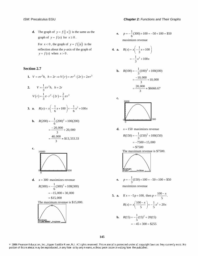
ISM: Precalculus EGU Chapter 2: Functions and Their Graphs
145
d. The graph of ( )y f x= is the same as the
graph of ( )y f x= for 0x ≥ .
For 0x < , the graph of ( )y f x= is the reflection about the y-axis of the graph of
( )y f x= when 0x > .
Section 2.7
1. ( ) ( )2 2 3, 2 2 2V r h h r V r r r rπ π π= = ⇒ = ⋅ =
2.
( ) ( )
2
2 3
1 , 231 223 3
V r h h r
V r r r r
π
π π
= =
= ⋅ ⋅ =
3. a. 21 1( ) 100 1006 6
R x x x x x⎛ ⎞= − + = − +⎜ ⎟⎝ ⎠
b. 21(200) (200) 100(200)620,000 20,000
340,000 $13,333.33
3
R = − +
−= +
= ≈
c.
600
16000
00
d. 300x = maximizes revenue 21(300) (300) 100(300)
615,000 30,000
$15,000
R = − +
= − +=
The maximum revenue is $15,000.
e. 1 (300) 100 50 100 $506
p = − + = − + =
maximizes revenue
4. a.
2
1( ) 1003
1 1003
R x x x
x x
⎛ ⎞= − +⎜ ⎟⎝ ⎠
= − +
b. 21(100) (100) 100(100)310,000 10,000
320,000 $6666.67
3
R = − +
−= +
= ≈
c.
3000
8000
0
d. 150x = maximizes revenue 21(150) (150) 100(150)
37500 15,000
$7500
R = − +
= − +=
The maximum revenue is $7500.
e. 1 (150) 100 50 100 $503
p = − + = − + =
maximizes revenue
5. a.
2
100If 5 100, then .5
100 1( ) 205 5
xx p p
xR x x x x
−= − + =
−⎛ ⎞= = − +⎜ ⎟⎝ ⎠
b. 21(15) (15) 20(15)545 300 $255
R = − +
= − + =

Chapter 2: Functions and Their Graphs ISM: Precalculus EGU
146
c.
100
600
00
d. 50x = maximizes revenue 21(50) (50) 20(50)
5500 1000 $500
R = − +
= − + =
The maximum revenue is $500.
e. 100 50 50 $105 5
p −= = =
maximizes revenue.
6. a.
2
500If 20 500, then .20
500 1( ) 2520 20
xx p p
xR x x x x
−= − + =
−⎛ ⎞= = − +⎜ ⎟⎝ ⎠
b. 21(20) (20) 25(20)2020 500 $480
R = − +
= − + =
c.
5000
4000
0
d. 250x = maximizes revenue 21(250) (250) 25(250)
203125 6250 $3125
R = − +
= − + =
The maximum revenue is $3125.
e. 500 250 250 $12.5020 20
p −= = =
maximizes revenue.
7. a. Let x = width and y = length of the rectangular area.
2 2 400400 2 200
2
P x yxy x
= + =−
= = −
Then
2
2
( ) (200 )
200
200
A x x x
x x
x x
= −
= −
= − +
b. We need 0 and 0 200 0 200x y x x> > ⇒ − > ⇒ >
So the domain of A is { }0 200x x< <
c. 100x = yards maximizes area
200
10000
00
8. a. Let x = length and y = width of the rectangular field.
2 30003000 11500
2 2
P x yxy x
= + =−
= = −
Then,
( ) 21 11500 15002 2
A x x x x x⎛ ⎞= − = −⎜ ⎟⎝ ⎠

ISM: Precalculus EGU Chapter 2: Functions and Their Graphs
147
b. 1500x = feet maximizes area
30000
1,250,000
0
9. a. The distance from d P to the origin is 2 2d x y= + . Since P is a point on the
graph of 2 8y x= − , we have: 2 2 2 4 2( ) ( 8) 15 64d x x x x x= + − = − +
b. 4 2(0) 0 15(0) 64 64 8d = − + = =
c. 4 2(1) (1) 15(1) 64 1 15 64
50 5 2 7.07
d = − + = − +
= = ≈
d.
10
−5
−10
40
e. d is smallest when 2.74x ≈ − and when 2.74x ≈ .
10. a. The distance from d P to (0, –1) is 2 2( 1)d x y= + + . Since P is a point on
the graph of 2 8y x= − , we have:
( )
2 2 2
22 2
4 2
( ) ( 8 1)
7
13 49
d x x x
x x
x x
= + − +
= + −
= − +
b. 4 2(0) 0 13(0) 49 49 7d = − + = =
c. 4 2( 1) ( 1) 13( 1) 49 37 6.08d − = − − − + = ≈
d.
4–4
10
0
e. d is smallest when 2.55x ≈ − and when 2.55x ≈ .
11. a. The distance from d P to the point (1, 0) is 2 2( 1)d x y= − + . Since P is a point on
the graph of y x= , we have:
( )22 2( ) ( 1) 1d x x x x x= − + = − +
where 0x ≥ .
b.
2
2
00
c. d is smallest when x is 0.50.

Chapter 2: Functions and Their Graphs ISM: Precalculus EGU
148
12. a. The distance from d P to the origin is 2 2d x y= + . Since P is a point on the
graph of 1yx
= , we have:
2 42 2
2 21 1 1( ) xd x x xx x x
+⎛ ⎞= + = + =⎜ ⎟⎝ ⎠
b.
5–5
8
0
c. d is smallest when x is 1 or –1.
13. By definition, a triangle has area 1 , base, height.2
A b h b h= = = From the figure,
we know that and .b x h y= = Expressing the area of the triangle as a function of x , we have:
( )3 41 1 1( )2 2 2
A x xy x x x= = = .
14. By definition, a triangle has area 1 , =base, height.2
A b h b h= = Because one
vertex of the triangle is at the origin and the other is on the x-axis, we know that
and .b x h y= = Expressing the area of the triangle as a function of x , we have:
( )2 31 1 9 1( ) 92 2 2 2
A x xy x x x x= = − = − .
15. a. ( )2 3( ) 16 16A x xy x x x x= = − = − +
b. Domain: { }0 4x x< <
c. The area is largest when x is approximately 2.31.
4
30
00
16. a. 2( ) 2 2 4A x xy x x= = −
b. 2( ) 2(2 ) 2( ) 4 2 4p x x y x x= + = + −
c. Graphing the area equation:
20
4
0
The area is largest when x is approximately 1.41.
d. Graphing the perimeter equation:
20
10
0
The perimeter is largest when x is approximately 1.79.

ISM: Precalculus EGU Chapter 2: Functions and Their Graphs
149
17. a. In Quadrant I, 2 2 24 4x y y x+ = → = − 2( ) (2 )(2 ) 4 4A x x y x x= = −
b. 2( ) 2(2 ) 2(2 ) 4 4 4p x x y x x= + = + −
c. Graphing the area equation:
2
10
00
The area is largest when x is roughly 1.41.
d. Graphing the perimeter equation:
2
12
00
The perimeter is largest when x is approximately 1.41.
18. a. 2( ) (2 )(2 ) 4A r r r r= =
b. ( ) 4(2 ) 8p r r r= =
19. a. circumference, total area, radius, side of squareC TAr x= == =
( )
square circle
2 2
22
22
5 2
5 2
2 10 4
Total Area area + area
( )
25 20 4
x
x
C r x r
x r
TA x x
x xx
π
π
−
−
= π = − ⇒ =
=
= + π
= + π
− += +
π
b. Since the lengths must be positive, we have: 10 4 0 and 0
4 10 and 02.5 and 0
x xx x
x x
− > >− > − >< >
Domain: { }0 2.5x x< <
c. The total area is smallest when x is approximately 1.40 meters.
2.5
8
00
20. a. circumference, total area, radius, side of equilateral triangle
C TAr x= == =
10 32 10 32
3height of the equilateral triangle is 2
xC r x r
x
−= π = − ⇒ =
π
triangle circle
2
22
22
Total Area area area
1 32 2
3 10 3( )4 2
3 100 60 94 4
x x r
xTA x x
x xx
= +
⎛ ⎞= + π⎜ ⎟⎜ ⎟
⎝ ⎠
−⎛ ⎞= + π =⎜ ⎟π⎝ ⎠
− ++
π
b. Since the lengths must be positive, we have: 10 3 0 and 0
3 10 and 010 and 03
x xx x
x x
− > >− > − >
< >
Domain: 1003
x x⎧ ⎫< <⎨ ⎬
⎩ ⎭

Chapter 2: Functions and Their Graphs ISM: Precalculus EGU
150
c. The area is smallest when x is approximately 2.08 meters.
3.330
8
0
21. a. Since the wire of length x is bent into a circle, the circumference is x . Therefore,
( )C x x= .
b. Since 2 ,2xC x r r= = π =π
.
2 22( )
2 4x xA x r ⎛ ⎞= π = π =⎜ ⎟π π⎝ ⎠
.
22. a. Since the wire of length x is bent into a square, the perimeter is x . Therefore,
( )P x x= .
b. Since 4 ,4xP x s s= = = , we have
2 22( )
4 16x xA x s ⎛ ⎞= = =⎜ ⎟
⎝ ⎠.
23. a. area, radius; diameter 2A r r= = = 2( ) (2 )( ) 2A r r r r= =
b. perimeterp = ( ) 2(2 ) 2 6p r r r r= + =
24. circumference, radius;length of a side of the triangle
C rx= ==
Since ABCΔ is equilateral, 32
xEM = .
Therefore, 3232
xOM OE
x r
= −
= −
In OAMΔ , 22
2
22 2 2
2
32 2
3 34 4
3
3
x xr r
xr x rx r
rx xxr
⎛ ⎞⎛ ⎞= + −⎜ ⎟⎜ ⎟⎝ ⎠ ⎝ ⎠
= + − +
=
=
Therefore, the circumference of the circle is 2 3( ) 2 2
33xC x r xπ⎛ ⎞
= π = π =⎜ ⎟⎝ ⎠
25. Area of the equilateral triangle
21 3 32 2 4
A x x x= ⋅ =
From problem 24, we have 2
2
3xr = .
Area inside the circle, but outside the triangle:
2 2
22
2
3( )4
33 4
33 4
A x r x
x x
x
= π −
= π −
⎛ ⎞π= −⎜ ⎟⎜ ⎟⎝ ⎠

ISM: Precalculus EGU Chapter 2: Functions and Their Graphs
151
26.
( ) ( )
( )
( )
2 2 21 2
2 22
2 2
2
30 40
900 1600
2500 50
d d d
d t t
d t t t
d t t t
= +
= +
= +
= =
d
d =40t
d =30t1
2
27. a.
( ) ( )
( ) ( ) ( )
2 2 21 2
2 22
2 2
2 2
2
2 30 3 40
2 30 3 40
4 120 900 9 240 1600
2500 360 13
d d d
d t t
d t t t
t t t t
t t
= +
= − + −
= − + −
= − + + − +
= − +
1 2 30d t= −
2 3 40d t= −
d
b. The distance is smallest at 0.072t ≈ hours.
28. radius of cylinder, height of cylinder,volume of cylinder
r hV= ==
2 2
2 2 2 2
2 4h hr R r R⎛ ⎞+ = ⇒ + =⎜ ⎟
⎝ ⎠
( )( )
2 2 22 2 2
2
2 2
2 3
2 2
44 4
4( )4
44
44
h R hr R r
V r h
R hV h h
R h h
h R hπ
−= − ⇒ =
= π
⎛ ⎞−= π⎜ ⎟⎜ ⎟
⎝ ⎠π
= −
= −
29. radius of cylinder, height of cylinder,volume of cylinder
r hV= ==
( )
By similar triangles: H H hR r
Hr R H hHr RH RhRh RH Hr
RH Hr Hrh HR R
−=
= −
= −= −
−= = −
2 2 2 1Hr rV r h r H H rR R
⎛ ⎞ ⎛ ⎞= π = π − = π −⎜ ⎟ ⎜ ⎟⎝ ⎠ ⎝ ⎠
30. a. The total cost of installing the cable along the road is 10x . If cable is installed x miles along the road, there are 5 x− miles between the road to the house and where the cable ends along the road.
House
Box
2d
5−x x 2 2 2
2
(5 ) 2 25 10 4
10 29
d x x x
x x
= − + = − + +
= − +
The total cost of installing the cable is: 2( ) 10 14 10 29C x x x x= + − +
Domain: { }0 5x x≤ ≤
b. ( ) ( )2(1) 10 1 14 1 10 1 29
10 14 20 $72.61
C = + − +
= + ≈
c. ( ) ( )2(3) 10 3 14 3 10 3 29
30 14 8 $69.60
C = + − +
= + ≈

Chapter 2: Functions and Their Graphs ISM: Precalculus EGU
152
d.
e. Using MINIMUM, the graph indicates that 2.96x ≈ miles results in the least cost.
31. a. The time on the boat is given by 1
3d
. The
time on land is given by 125
x− .
x
2
12–x
d1
Islande
TownP
2 2 21 2 4d x x= + = +
The total time for the trip is: 2
112 12 4( )5 3 5 3
dx x xT x − − += + = +
b. Domain: { }0 12x x≤ ≤
c. 212 4 4 4(4)
5 38 20 3.09 hours5 3
T − += +
= + ≈
d. 212 8 8 4(8)
5 34 68 3.55 hours5 3
T − += +
= + ≈
32. Consider the diagrams shown below.
There is a pair of similar triangles in the diagram. Since the smaller triangle is similar to the larger triangle, we have the proportion
4 1 116 4 4
r r r hh h= ⇒ = ⇒ =
Substituting into the volume formula for the conical portion of water gives
( )2
2 31 1 1 13 3 4 48
V h r h h h hπ π π⎛ ⎞= = =⎜ ⎟⎝ ⎠
.
Chapter 2 Review
1. This relation represents a function. Domain = {–1, 2, 4}; Range = {0, 3}.
2. This relation does not represent a function, since 4 is paired with two different values.
3. 23( )
1xf x
x=
−
a. 23(2) 6 6(2) 2
4 1 3(2) 1f = = = =
−−
b. 23( 2) 6 6( 2) 2
4 1 3( 2) 1f − − −− = = = = −
−− −

ISM: Precalculus EGU Chapter 2: Functions and Their Graphs
153
c. 2 23( ) 3( )
( ) 1 1x xf x
x x− −− = =
− − −
d. 2 23 3( )
1 1x xf x
x x−⎛ ⎞− = − =⎜ ⎟− −⎝ ⎠
e.
( )
2
2
2
3( 2)( 2)( 2) 1
3 64 4 1
3 24 3
xf xx
xx x
xx x
−− =
− −−=
− + −−
=− +
f. 2 23(2 ) 6(2 )
(2 ) 1 4 1x xf x
x x= =
− −
4. 2
( )1
xf xx
=+
a. 22 4(2)
2 1 3f = =
+
b. ( )22 4( 2) 4
2 1 1f
−− = = = −
− + −
c. 2 2( )( )1 1
x xf xx x
−− = =
− + − +
d. 2 2
( )1 1
x xf xx x
−− = − =+ +
e. ( )22 2( 2)( 2)
( 2) 1 1xxf x
x x−−
− = =− + −
f. 2 2(2 ) 4(2 )
(2 ) 1 2 1x xf x
x x= =
+ +
5. 2( ) 4f x x= −
a. 2(2) 2 4 4 4 0 0f = − = − = =
b. ( )2( 2) 2 4 4 4 0 0f − = − − = − = =
c. 2 2( ) ( ) 4 4f x x x− = − − = −
d. 2( ) 4f x x− = − −
e. 2
2
2
( 2) ( 2) 4
4 4 4
4
f x x
x x
x x
− = − −
= − + −
= −
f.
( )
2 2
2 2
(2 ) (2 ) 4 4 4
4 1 2 1
f x x x
x x
= − = −
= − = −
6. 2( ) 4f x x= −
a. 2(2) 2 4 4 4 0 0f = − = − = =
b. ( )2( 2) 2 4 4 4 0 0f − = − − = − = =
c. 2 2( ) ( ) 4 4f x x x− = − − = −
d. 2( ) 4f x x− = − −
e. 2
2
2
( 2) ( 2) 4
4 4 4
4
f x x
x x
x x
− = − −
= − + −
= −
f.
( )
2 2
2 2
(2 ) (2 ) 4 4 4
4 1 4 1
f x x x
x x
= − = −
= − = −
7. 2
24( ) xf x
x−=
a. 2
22 4 4 4 0(2) 0
4 42f − −= = = =
b. ( )
( )
2
2
2 4 4 4 0( 2) 04 42
f− − −− = = = =
−
c. 2 2
2 2( ) 4 4( )
( )x xf x
x x− − −− = =
−
d. 2 2 2
2 2 24 4 4( ) x x xf x
x x x⎛ ⎞− − −− = − = = −⎜ ⎟⎝ ⎠
e.
( )
2 2
2 2
2
2 2
( 2) 4 4 4 4( 2)( 2) ( 2)
44( 2) ( 2)
x x xf xx x
x xx xx x
− − − + −− = =− −
−−= =− −

Chapter 2: Functions and Their Graphs ISM: Precalculus EGU
154
f.
( )
2 2
2 2
2 2
2 2
(2 ) 4 4 4(2 )(2 ) 4
4 1 14
x xf xx x
x xx x
− −= =
− −= =
8. 3
2( )9
xf xx
=−
a. 3
22 8 8 8(2)
4 9 5 52 9f = = = = −
− −−
b. ( )
( )
3
2
2 8 8 8(2)4 9 5 52 9
f− − −= = = =
− −− −
c. 3 3
2 2( )( )
( ) 9 9x xf x
x x− −− = =
− − −
d. 3 3
2 2( )9 9
x xf xx x
−− = − =− −
e. 3
2
3
2
3
2
( 2)( 2)( 2) 9
( 2)4 4 9
( 2)4 5
xf xx
xx x
xx x
−− =
− −
−=
− + −−
=− −
f. 3 3
2 2(2 ) 8(2 )
(2 ) 9 4 9x xf x
x x= =
− −
9. 2( )9
xf xx
=−
The denominator cannot be zero: 2 9 0
( 3)( 3) 03 or 3
xx x
x
− ≠+ − ≠
≠ −
Domain: { }3, 3x x x≠ − ≠
10. 23( )2
xf xx
=−
The denominator cannot be zero: 2 0
2x
x− ≠
≠
Domain: { }2x x ≠
11. ( ) 2f x x= − The radicand must be non-negative: 2 0
2xx
− ≥≤
Domain: { } ( ]2 or , 2x x ≤ −∞
12. ( ) 2f x x= + The radicand must be non-negative:
2 02
xx
+ ≥≥ −
Domain: { } [ )2 or 2,x x ≥ − − ∞
13. ( ) xf xx
=
The radicand must be non-negative and the denominator cannot be zero: 0x > Domain: { } ( )0 or 0,x x > ∞
14. ( )x
g xx
=
The denominator cannot be zero: 0x ≠
Domain: { }0x x ≠
15. 2( )2 3xf x
x x=
+ −
The denominator cannot be zero:
( )( )
{ }
2 2 3 03 1 03 or 1
Domain: 3, 1
x xx x
x
x x x
+ − ≠
+ − ≠
≠ −
≠ − ≠
16. ( ) 213 4
F xx x
=− −
The denominator cannot be zero:
( )( )
{ }
2 3 4 01 4 01 or 4
Domain: 1, 4
x xx x
x
x x x
− − ≠
+ − ≠
≠ −
≠ − ≠

ISM: Precalculus EGU Chapter 2: Functions and Their Graphs
155
17. ( ) 2 ( ) 3 1f x x g x x= − = +
( )( )( ) ( )2 3 1 2 3
f g x f x g xx x x
+ = +
= − + + = +
Domain: { } is any real numberx x
( )( )
( )( ) ( )
2 3 12 3 1
4 1
f g x f x g x
x xx x
x
− = −
= − − +
= − − −= − +
Domain: { } is any real numberx x
( )( )( )
2
2
( )( ) ( )
2 3 1
6 2 3
3 5 2
f g x f x g x
x x
x x x
x x
⋅ = ⋅
= − +
= + − −
= − + +
Domain: { } is any real numberx x
( )( )
2( )3 1
f xf xxg xg x
−⎛ ⎞ = =⎜ ⎟ +⎝ ⎠
3 1 013 13
x
x x
+ ≠
≠ − ⇒ ≠ −
1Domain: 3
x x⎧ ⎫≠ −⎨ ⎬⎩ ⎭
18. ( ) 2 1 ( ) 2 1f x x g x x= − = +
( )( )( ) ( )2 1 2 14
f g x f x g xx xx
+ = +
= − + +=
Domain: { } is any real numberx x
( )( )
( )( ) ( )
2 1 2 12 1 2 1
2
f g x f x g x
x xx x
− = −
= − − +
= − − −= −
Domain: { } is any real numberx x
( )( )( )
2
2
( )( ) ( )
2 1 2 1
4 2 2 1
4 1
f g x f x g x
x x
x x x
x
⋅ = ⋅
= − +
= + − −
= −
Domain: { } is any real numberx x
( )( )
2 1( )2 1
f xf xxg xg x
−⎛ ⎞ = =⎜ ⎟ +⎝ ⎠
12 1 0 2 12
x x x+ ≠ ⇒ ≠ − ⇒ ≠ −
{ }12Domain: x x ≠ −
19. 2( ) 3 1 ( ) 3f x x x g x x= + + =
( )2
2
( )( ) ( )
3 1 3
3 4 1
f g x f x g x
x x x
x x
+ = +
= + + +
= + +
Domain: { }is any real numberx x
( )2
2
( )( ) ( )
3 1 3
3 2 1
f g x f x g x
x x x
x x
− = −
= + + −
= − +
Domain: { }is any real numberx x
( )( )( )2
3 2
( )( ) ( )
3 1 3
9 3 3
f g x f x g x
x x x
x x x
⋅ = ⋅
= + +
= + +
Domain: { }is any real numberx x
( )( )
23 1( )3
f xf x xxg xg x
+ +⎛ ⎞ = =⎜ ⎟⎝ ⎠
3 0 0x x≠ ⇒ ≠ { }Domain: 0x x ≠
20. 2( ) 3 ( ) 1f x x g x x x= = + +
( )2
2
( )( ) ( )
3 1
4 1
f g x f x g x
x x x
x x
+ = +
= + + +
= + +
Domain: { }is any real numberx x
( )( )2
2
( )( ) ( )
3 1
2 1
f g x f x g x
x x x
x x
− = −
= − + +
= − + −
Domain: { }is any real numberx x
( )( )( )2
2 3
( )( ) ( )
3 1
3 3 3
f g x f x g x
x x x
x x x
⋅ = ⋅
= + +
= + +
Domain: { }is any real numberx x

Chapter 2: Functions and Their Graphs ISM: Precalculus EGU
156
( )( ) 2
3( )1
f xf xxg g x x x
⎛ ⎞ = =⎜ ⎟ + +⎝ ⎠
2
2
1 0
1 0
x x
x x
+ + ≠
+ + ≠
Since the discriminant is ( )( )21 4 1 1 3 0− = − < , 2 1x x+ + will never equal 0.
Domain: { } is any real numberx x
21. 1 1( ) ( )1
xf x g xx x
+= =−
( )
( ) ( )( )
( )
( )
2
2
( )( ) ( )1 11
1 1 11
11
2 11
f g x f x g xxx xx x x
x x
x x xx x
x xx x
+ = +
+= +−
+ + −=
−
+ + −=−
+ −=−
{ }Domain: 0, 1x x x≠ ≠
( )
( ) ( )( )
( )
( )
2
2
( )( ) ( )1 11
1 1 11
11
11
f g x f x g xxx xx x x
x x
x x xx x
xx x
− = −
+= −−
+ − −=
−
+ − +=−
+=−
{ }Domain: 0, 1x x x≠ ≠
( ) ( )1 1 1( )( ) ( )1 1
x xf g x f x g xx x x x
+ +⎛ ⎞⎛ ⎞⋅ = ⋅ = =⎜ ⎟⎜ ⎟− −⎝ ⎠⎝ ⎠
{ }Domain: 0, 1x x x≠ ≠
( )( )
1( 1)11( )
1 1 1 1
xf xf x xx xxx
g x xg xx
+++⎛ ⎞ ⎛ ⎞⎛ ⎞−= = = =⎜ ⎟⎜ ⎟⎜ ⎟ − −⎝ ⎠⎝ ⎠⎝ ⎠
{ }Domain: 0, 1x x x≠ ≠
22. 1 3( ) ( )3
f x g xx x
= =−
( )( )
( )
( ) ( )
( )( ) ( )
3 31 33 33 9 4 9
3 3
f g x f x g x
x xx x x xx x xx x x x
+ = +
+ −= + =
− −
+ − −= =− −
{ }Domain: 0, 3x x x≠ ≠
( )
( )( ) ( )
( )
1 3( )( ) ( )3
3 3 3 93 3
2 93
f g x f x g xx x
x x x xx x x x
xx x
− = − = −−
− − − += =− −
− +=−
{ }Domain: 0, 3x x x≠ ≠
( ) ( )1 3 3( )( ) ( )
3 3f g x f x g x
x x x x⎛ ⎞⎛ ⎞⋅ = ⋅ = =⎜ ⎟⎜ ⎟− −⎝ ⎠⎝ ⎠
{ }Domain: 0, 3x x x≠ ≠
( )( )
( )
113( )
3 3 3
3 3
f xf xxxg xg x
xx
x
⎛ ⎞ ⎛ ⎞⎛ ⎞−= = = ⎜ ⎟⎜ ⎟⎜ ⎟ −⎝ ⎠⎝ ⎠⎝ ⎠
=−
{ }Domain: 0, 3x x x≠ ≠
23. 2( ) 2 1f x x x= − + +
( ) ( )
( ) ( ) ( )
( )
( )
2 2
2 2 2
2 2 2
2
2 1 2 1
2 2 1 2 1
2 4 2 1 2 1
4 2 14 2
4 2 1
f x h f xh
x h x h x xh
x xh h x h x xh
x xh h x h x xh
h x hxh h hh h
x h
+ −
− + + + + − − + +=
− + + + + + + − −=
− − − + + + + − −=
− − +− − += =
= − − +

ISM: Precalculus EGU Chapter 2: Functions and Their Graphs
157
24. 2( ) 3 2 4f x x x= − + ( ) ( )
( ) ( ) ( )
( )
( )
2 2
2 2 2
2 2 2
2
3 2 4 3 2 4
3 2 2 2 4 3 2 4
3 6 3 2 2 4 3 2 4
6 3 26 3 2
6 3 2
f x h f xh
x h x h x xh
x xh h x h x xh
x xh h x h x xh
h x hxh h hh h
x h
+ −
+ − + + − − +=
+ + − − + − + −=
+ + − − + − + −=
+ −+ −= =
= + −
25. a. Domain:{ }4 3x x− ≤ ≤
Range: { }3 3y y− ≤ ≤
b. x-intercept: ( )0,0 ; y-intercept: ( )0,0
c. ( )2 1f − = −
d. ( ) 3f x = − when x = –4
e. ( ) 0f x > when 0 3x< ≤
f. To graph ( )3y f x= − , shift the graph of f horizontally 3 units to the right.
g. To graph 12
y f x⎛ ⎞= ⎜ ⎟⎝ ⎠
, stretch the graph of
f horizontally by a factor of 2.
h. To graph ( )y f x= − , reflect the graph of f vertically about the y-axis.
26. a. Domain: { }5 4x x− ≤ ≤
Range: { }3 1y y− ≤ ≤
b. ( 1) 1g − =
c. x-intercepts: ( ) ( )0,0 , 4,0 ;
y-intercept: ( )0,0
d. ( ) 3g x = − when 3x =
e. ( ) 0g x > when 5 0x− ≤ <

Chapter 2: Functions and Their Graphs ISM: Precalculus EGU
158
f. To graph ( )2y g x= − , shift the graph of g horizontally 2 units to the right.
g. To graph ( ) 1y g x= + , shift the graph of g vertically up 1 unit.
h. To graph ( )2y g x= , stretch the graph of g vertically by a factor of 2.
27. a. Domain: { }4 4x x− ≤ ≤
Range: { }3 1y y− ≤ ≤
b. Increasing: ( ) ( )4, 1 and 3,4− − ; Decreasing: (–1, 3)
c. Local minimum is 3− when 3x = ; Local maximum is 1 when 1x = − . Note that 4x = and 4x = − do not yield local extrema because there is no open interval that contains either value.
d. The graph is not symmetric with respect to the x-axis, the y-axis or the origin.
e. The function is neither even nor odd.
f. x-intercepts: ( ) ( ) ( )2,0 , 0,0 , 4,0− ,
y-intercept: ( )0,0
28. a. Domain: { }is any real numberx x
Range: { }is any real numbery y
b. Increasing: ( ), 2−∞ − and ( )2,∞ ;
Decreasing: ( )2, 2−
c. Local minimum is 1− at 2x = ; Local maximum is 1 at 2x = −
d. The graph is symmetric with respect to the origin.
e. The function is odd.
f. x-intercepts: ( ) ( ) ( )3,0 , 0,0 , 3,0− ;
y-intercept: ( )0,0
29. 3( ) 4f x x x= −
( )3 3
3
( ) ( ) 4( ) 4
4 ( )
f x x x x x
x x f x
− = − − − = − +
= − − = −
f is odd.
30. 2
44( )1
xg xx
+=+
2 2
4 44 ( ) 4( ) ( )1 ( ) 1
x xg x g xx x
+ − +− = = =+ − +
g is even.
31. 4 21 1( ) 1h xx x
= + +
4 2 4 21 1 1 1( ) 1 1 ( )
( ) ( )h x h x
x x x x− = + + = + + =
− −
h is even.

ISM: Precalculus EGU Chapter 2: Functions and Their Graphs
159
32. 3( ) 1F x x= − 3 3( ) 1 ( ) 1 ( ) or ( )F x x x F x F x− = − − = + ≠ −
F is neither even nor odd.
33. 3( ) 1G x x x= − + 3
3
( ) 1 ( ) ( )
1 ( ) or ( )
G x x x
x x G x G x
− = − − + −
= + − ≠ −
G is neither even nor odd.
34. 2( ) 1H x x x= + + 2
2
( ) 1 ( ) ( )
1 ( ) or ( )
H x x x
x x H x H x
− = + − + −
= − + ≠ −
H is neither even nor odd.
35. 2( )1
xf xx
=+
2 2( ) ( )1 ( ) 1
x xf x f xx x
− −− = = = −+ − +
f is odd.
36. 2
31( ) xg x
x+=
2 2 2
3 3 31 ( ) 1 1( ) ( )
( )x x xg x g x
x x x+ − + +− = = = − = −− −
g is odd.
37. ( ) 32 5 1f x x x= − + on the interval ( )3,3− Use MAXIMUM and MINIMUM on the graph of 3
1 2 5 1y x x= − + .
20
−3 3
−20
20
−3 3
−20 local maximum at: ( )0.91,4.04− ;
local minimum at: ( )0.91, 2.04−
f is increasing on: ( ) ( )3, 0.91 and 0.91,3− − ;
f is decreasing on: ( )0.91,0.91−
38. ( ) 3 3 5f x x x= − + − on the interval ( )3,3− Use MAXIMUM and MINIMUM on the graph of 3
1 3 5y x x= − + − .
20
−3 3
−20
20
−3 3
−20 local maximum at: ( )1, 3− ;
local minimum at: ( )1, 7− −
f is increasing on: ( )1,1− ;
f is decreasing on: ( ) ( )3, 1 and 1,3− −
39. ( ) 4 32 5 2 1f x x x x= − + + on the interval ( )2,3− Use MAXIMUM and MINIMUM on the graph of 4 3
1 2 5 2 1y x x x= − + + .
−2
20
3
−10
−2
20
3
−10
−2
20
3
−10 local maximum at: ( )0.41,1.53 ;
local minima at: ( )0.34,0.54− , ( )1.80, 3.56−
f is increasing on: ( ) ( )0.34,0.41 and 1.80,3− ;
f is decreasing on: ( ) ( )2, 0.34 and 0.41,1.80− −
40. ( ) 4 33 4 3f x x x x= − + − + on the interval ( )2,3− Use MAXIMUM and MINIMUM on the graph of 4 3
1 3 4 3y x x x= − + − + .
5
−5
−2 3
5
−5
−2 3

Chapter 2: Functions and Their Graphs ISM: Precalculus EGU
160
5
−5
−2 3
local maxima at: ( )0.59, 4.62− , ( )2,3 ;
local minimum at: ( )0.84,0.92
f is increasing on: ( ) ( )2, 0.59 and 0.84, 2− − ;
f is decreasing on: ( ) ( )0.59,0.84 and 2,3−
41. 2( ) 8f x x x= −
a. ( ) ( )( )
( )
2 28 2 2 8 1 1(2) (1)2 1 1
32 2 7 23
f f − − −−=
−= − − =
b. ( ) ( )( )
( )
2 28 1 1 8 0 0(1) (0)1 0 1
8 1 0 7
f f − − −−=
−= − − =
c. ( ) ( )( )
( )
2 28 4 4 8 2 2(4) (2)4 2 2
128 4 30 94 472 2
f f − − −−=
−− −
= = =
42. 3( ) 2f x x x= +
a. ( ) ( )( )
( )
3 32 2 2 2 1 1(2) (1)2 1 1
16 2 3 15
f f + − +−=
−= + − =
b. ( ) ( )( )
( )
3 32 1 1 2 0 0(1) (0)1 0 1
2 1 0 3
f f + − +−=
−= + − =
c. ( ) ( )( )
( )
3 32 4 4 2 2 2(4) (2)4 2 2
128 4 18 114 572 2
f f + − +−=
−+ −
= = =
43. ( ) 2 5f x x= − 2 5 ( 8)( ) (2) 5 10
2 2 25( 2) 5
2
xf x f xx x x
xx
− − −− − += =− − −
− −= = −
−
44. 2( ) 2 7f x x= + 2 2( ) (2) 2 7 15 2 8
2 2 22( 2)( 2) 2 4
2
f x f x xx x x
x x xx
− + − −= =− − −
− += = +
−
45. 2( ) 3 4f x x x= − 2
2
2
( ) (2) 3 4 ( 10)2 2
4 3 102
(4 3 10)2
(4 5)( 2)2
4 5
f x f x xx x
x xx
x xx
x xx
x
− − − −=
− −− + +
=−
− − −=
−− + −
=−
= − −
46. 2( ) 3 2f x x x= − + 2
2
( ) (2) 3 2 02 2
3 22
( 2)( 1)2
1
f x f x xx x
x xx
x xx
x
− − + −=− −
− +=−
− −=
−= −
47. (b) passes the Vertical Line Test and is therefore a function.
48. (a) and (b) both pass the Vertical Line Test and are therefore functions.
49. ( ) 2 5f x x= −

ISM: Precalculus EGU Chapter 2: Functions and Their Graphs
161
50. ( ) 4 7g x x= − +
51. 4( ) 65
h x x= −
52. 1( ) 13
F x x= − +
53. ( )f x x=
54. 3( )f x x=
55. ( ) 4F x x= −
Using the graph of y x= , vertically shift the graph downward 4 units.
Intercepts: (–4,0), (4,0), (0,–4) Domain: { }is any real numberx x
Range: { }4y y ≥ −
56. ( ) 4f x x= +
Using the graph of y x= , vertically shift the graph upward 4 units.
Intercepts: (0, 4) Domain: { }is any real numberx x
Range: { }4y y ≥

Chapter 2: Functions and Their Graphs ISM: Precalculus EGU
162
57. ( ) 2g x x= −
Reflect the graph of y x= about the x-axis and vertically stretch the graph by a factor of 2.
Intercepts: (0, 0) Domain: { } is any real numberx x
Range: { }0y y ≤
58. 1( )2
g x x=
Using the graph of y x= , vertically shrink the
graph by a factor of 12
.
Intercepts: (0, 0) Domain: { } is any real numberx x
Range: { }0y y ≥
59. ( ) 1h x x= −
Using the graph of y x= , horizontally shift the graph to the right 1 unit.
Intercept: (1, 0) Domain: { }1x x ≥ ; Range: { }0y y ≥
60. ( ) 1h x x= −
Using the graph of y x= , vertically shift the graph downward 1 unit.
Intercepts: (1, 0), (0, –1) Domain: { }0x x ≥ ; Range: { }1y y ≥ −
61. ( ) 1 1( 1)f x x x= − = − −
Reflect the graph of y x= about the y-axis and horizontally shift the graph to the right 1 unit.
Intercepts: (1 ,0), (0,1) Domain: { }1x x ≤
Range: { }0y y ≥

ISM: Precalculus EGU Chapter 2: Functions and Their Graphs
163
62. ( ) 3f x x= − +
Using the graph of y x= , horizontally shift the graph to the left 3 units, and reflect on the x-axis.
Intercepts: (–3, 0), ( )0, 3−
Domain: { }3x x ≥ −
Range: { }0y y ≤
63. 2( ) ( 1) 2h x x= − +
Using the graph of 2y x= , horizontally shift the graph to the right 1 unit and vertically shift the graph up 2 units.
Intercepts: (0, 3) Domain: { } is any real numberx x
Range: { }2y y ≥
64. 2( ) ( 2) 3h x x= + −
Using the graph of 2y x= , horizontally shift the graph to the left 2 units and vertically shift the graph down 3 units.
Intercepts: (0, 1), ( ) ( )2 3, 0 , 2 3, 0− + − −
Domain: { }is any real numberx x
Range: { }3y y ≥ −
65. 3( ) 3( 1) 1g x x= − +
Using the graph of 3y x= , horizontally shift the graph to the right 1 unit vertically stretch the graph by a factor of 3, and vertically shift the graph up 1 unit.
−5
y
x5
5
−5
(0, −2)
(1, 1)
(2, 4)
3 91 , 03
⎛ ⎞−⎜ ⎟
⎝ ⎠
Intercepts: (0,–2), 3 91 , 03
⎛ ⎞−⎜ ⎟
⎝ ⎠
Domain: { }is any real numberx x
Range: { }is any real numbery y

Chapter 2: Functions and Their Graphs ISM: Precalculus EGU
164
66. 3( ) 2( 2) 8g x x= − + −
Using the graph of 3y x= , horizontally shift the graph to the left 2 units, vertically stretch the graph by a factor of 2, reflect about the x-axis, and vertically shift the graph down 8 units.
−9
y
x
−5(−3, −6)
(−2, −8)(−1, −10)
( )32 4, 0− −
Intercepts: (0,–24), ( )32 4, 0− −
Domain: { } is any real numberx x
Range: { } is any real numbery y
67. 3 if 2 1
( )1 if 1
x xf x
x x− < ≤⎧
= ⎨ + >⎩
a. Domain: { }2x x > −
b. x-intercept: ( )0,0 y-intercept: (0,0)
c. Graph:
d. Range: { }6y > −
68. 1 if 3 0
( )3 1 if 0x x
f xx x− − < <⎧
= ⎨ − ≥⎩
a. Domain: { }3x x > −
b. x-intercept: 1 ,03
⎛ ⎞⎜ ⎟⎝ ⎠
y-intercept: (0, –1)
c. Graph:
d. Range: { }4y > −
69. if 4 0
( ) 1 if 03 if 0
x xf x x
x x
− ≤ <⎧⎪= =⎨⎪ >⎩
a. Domain: { }4x x ≥ −
b. x-intercept: none y-intercept: (0, 1)
c. Graph:
d. Range: { }4, 0y y y≥ − ≠
70. 2 if 2 2( )
2 1 if 2x xf x
x x⎧ − ≤ ≤⎪= ⎨
− >⎪⎩
a. Domain: { }2x x ≥ −
b. x-intercept: (0, 0) y-intercept: (0, 0)

ISM: Precalculus EGU Chapter 2: Functions and Their Graphs
165
c. Graph:
d. Range: { }0y y ≥
71. (4) 5f = − gives the ordered pair (4, 5)−
( )0 3f = gives (0) 3 gives (0,3)f =
Finding the slope: 3 ( 5) 8 20 4 4
m − −= = = −
− −
Using slope-intercept form: ( ) 2 3f x x= − +
72. 4, ( 2) 2m g= − − = gives the ordered pair ( 2, 2)− . Using point-slope form:
2 4( ( 2))2 4 8
4 6( ) 4 6
y xy x
y xg x x
− = − − −− = − −
= − −= − −
73. 5( ) and (1) 46 2Axf x f
x+= =−
(1) 5 46(1) 2
5 44
5 1611
A
A
AA
+=
−+ =
+ ==
74. 28( ) and ( 1) 0Ag x g
x x= + − =
28 0
1 ( 1)8 0
8
A
AA
+ =− −
− + ==
75. We have the points ( ) ( )1 1, 0,30h T = and
( ) ( )2 2, 10000,5h T = . 5 30 25slope 0.0025
10000 0 10000Th
Δ − −= = = = −Δ −
Using the point-slope formula yields ( ) ( )
( )
1 1 30 0.0025 030 0.0025 0.0025 30
0.0025 30, 0 10,000
T T m h h T hT h T hT h h x
− = − ⇒ − = − −
− = − ⇒ = − +
= − + ≤ ≤
76. We have the point ( ) ( )1 1, 20,80t v = and slope 5m= = Using the point-slope formula yields
( ) ( )
( )
1 1 80 5 2080 5 100 5 20
5 20
v v m t t v tv t v tv t t
− = − ⇒ − = −
− = − ⇒ = −
= −
After 30 seconds, ( ) ( )30 5 30 20 150 20 130 ft. per sec.v = − = − =
77. 24S r= π ; 343
V rπ=
Let 2R r= , 2 = new surface areaS , and
2 new volumeV = .
( )( ) ( )
222
2 2
4 4 2
4 4 4 4
4
S R r
r r
S
π π
π π
= =
= =
=
( )
( )
332
3 3
4 4 23 34 48 83 38
V R r
r r
V
π π
π π
= =
⎛ ⎞= = ⎜ ⎟⎝ ⎠
=
Thus, if the radius of the sphere doubles, the surface area is 4 times as large and the volume is 8 times as large as for the original sphere.
78. a. The printed region is a rectangle. Its area is given by
( )( ) ( )( )( ) ( )( )
length width 11 2 8.5 2
11 2 8.5 2
A x x
A x x x
= = − −
= − −

Chapter 2: Functions and Their Graphs ISM: Precalculus EGU
166
b. For the domain of ( ) ( )( )11 2 8.5 2A x x x= − −
recall that the dimensions of a rectangle must be non-negative.
0x ≥ and 11 2 02 11
5.5
xxx
− ≥− ≥ −
≤
and 8.5 2 0
2 8.5
4.25
x
x
x
− ≥
− ≥
≤
The domain is { }| 0 4.25x x≤ ≤ .
The range of ( ) ( ) ( )11 2 8.5 2A x x x= − − is given by
( ) ( )4.25 0 0 93.5A A A A≤ ≤ ⇒ ≤ ≤
c. ( ) ( )( ) ( )( )2
1 11 2 1 8.5 2 1
9 6.5 58.5 in
A = − −
= ⋅ =
( ) ( )( ) ( )( )2
1.2 11 2 1.2 8.5 2 1.2
8.6 6.1 52.46 in
A = − −
= ⋅ =
( ) ( )( ) ( )( )2
1.5 11 2 1.5 8.5 2 1.5
8 5.5 44 in
A = − −
= ⋅ =
d. ( ) ( )1 11 2 8.5 2y x x= − ∗ −
e. Using TRACE, 70 when 0.643 inchesA x≈ ≈
50 when 1.28 inchesA x= ≈
79. 3 , width; depthS kxd x d= = = In the diagram, depth = length of the rectangle. Therefore, we have
2 22
2 2
2 2
2
32 2
94 4
36
36
d x
d x
d x
d x
⎛ ⎞ ⎛ ⎞+ =⎜ ⎟ ⎜ ⎟⎝ ⎠ ⎝ ⎠
+ =
+ =
= −
( ) ( ) ( )3 3/ 22 236 36S x kx x kx x= − = −
Domain: { } 0 6x x< <
80. a. We are given that the volume is 100 cubic feet, so we have
22
100100V r h hr
ππ
= = ⇒ =
The amount of material needed to construct the drum is the surface area of the barrel. The cylindrical body of the barrel can be viewed as a rectangle whose dimensions are given by 2πr
h
( )
top bottom body
2 2 2
2 22
area area area
2 2 2100 2002 2 2
A
r r rh r rh
A r r r rrr
π π π π π
π π ππ
= + +
= + + = +
⎛ ⎞= + = +⎜ ⎟⎝ ⎠
b. ( ) ( )2
2
2003 2 33
20018 123.22 ft3
A π
π
= +
= + ≈
c. ( ) ( )2
2
2004 2 44
32 50 150.53 ft
A π
π
= +
= + ≈
d. ( ) ( )2
2
2005 2 55
50 40 197.08 ft
A π
π
= +
= + ≈
e. Graphing:
The minimum value occurs when
2.52 feetr ≈ .

ISM: Precalculus EGU Chapter 2: Functions and Their Graphs
167
81. a. The relation is a function. Each HS GPA value is paired with exactly one College GPA value.
b. Scatter diagram:
42.5
4
2.25 c. Using the LINear REGression program, the
line of best fit is: 0.964 0.072G x= +
d. As the high school GPA increases by 0.1 point, the college GPA increases by 0.0964 point.
e. ( ) 0.964 0.072G x x= +
f. Domain: { }0 4x x≤ ≤
g. ( ) ( )( )3.23 0.964 3.23 0.072 3.19G = + ≈ The college GPA is approximately 3.19.
82. Let p = the monthly payment in dollars, and B = the amount borrowed in dollars. Consider the ordered pair ( ),B p . We can use the points
( )0,0 and ( )130000,854 . Now compute the slope:
854 0 854slope 0.0065692130000 0 130000
yx
Δ −= = = ≈Δ −
Therefore we have the linear function ( ) 0.0065692 0 0.0065692p B B B= + =
If 165000B = , then ( )( )0.0065692 165000 $1083.92p = ≈ .
83. Let R = the revenue in dollars, and g = the number of gallons of gasoline sold. Consider the ordered pair ( ),g R . We can use
the points ( )0,0 and ( )13.5,28.89 . Now compute the slope:
28.89 0 28.89slope 2.1413.5 0 13.5
yx
Δ −= = = ≈Δ −
Therefore we have the linear function ( ) 2.14 0 2.14R g g g= + = .
If 11.2g = , then ( )( )2.14 11.2 $23.97R = = .
84. Since there are 200 feet of border, we know that 2 2 200x y+ = . The area is to be maximized, so A x y= ⋅ . Solving the perimeter formula for y :
2 2 200 2 200 2 100x y y x y x+ = → = − → = − The area function is:
2( ) (100 ) 100A x x x x x= − = − + The maximum value occurs at the vertex:
The pond should be 50 feet by 50 feet for maximum area.
85. Let x represent the length and y represent the width of the rectangle. 2 2 20 10x y y x+ = → = − .
16 (10 ) 16x y x x⋅ = → − = . Solving the area equation:
2 210 16 10 16 0( 8)( 2) 0 8 or 2
x x x xx x x x
− = → − + =− − = → = =
The length and width of the rectangle are 8 feet by 2 feet.
86. The area function is: 2( ) (10 ) 10A x x x x x= − = − +
The maximum value occurs at the vertex:
The maximum area is:
2(5) (5) 10(5)25 50 25 square units
A = − += − + =
(x,10-x)
10
10(x,0)
(0,10-x)

Chapter 2: Functions and Their Graphs ISM: Precalculus EGU
168
87. 2( ) 4.9 617.40 19,600C x x x= − + ; 4.9, 617.40, 19,600.a b c= = − =
Since 4.9 0,a = > the graph opens up, so the vertex is a minimum point.
a. The minimum marginal cost occurs at 63x = .
b. The minimum marginal cost is
( )
( ) ( )( )2
632
4.9 63 617.40 63 19600$151.90
bC Ca
−⎛ ⎞ =⎜ ⎟⎝ ⎠
= − +
=
88. Let ( )3,1P = and ( ) ( ), ,Q x y x x= = .
( ) ( ) ( )
( ) ( ) ( )
( )
2 2
2 22
2 2
2 2
, 3 1
3 1
6 9 2 1
2 8 10
d P Q x x
d x x x
x x x x
d x x x
= − + −
= − + −
= − + + − +
= − +
Since ( )2 22 8 10d x x x= − + is a quadratic function with a = 2 > 0, the vertex corresponds to the minimum value for the function.
The vertex occurs at 2x = . Therefore the point Q on the line y x= will be closest to the point
( )3,1P = when ( )2, 2Q = .
P(3,1)
Q(x, x) d
89. Let ( )4,1P = and ( ) ( ), , 1Q x y x x= = + .
( ) ( ) ( )
( ) ( )
( )
2 2
22 2
2 2
2 2
, 4 1 1
4
8 16
2 8 16
d P Q x x
d x x x
x x x
d x x x
= − + + −
→ = − +
= − + +
∴ = − +
Since ( )2 22 8 16d x x x= − + is a quadratic function with a = 2 > 0, the vertex corresponds to the minimum value for the function.
The vertex occurs at 2x = . Therefore the point Q on the line 1y x= + will be closest to the point ( )4,1P = when ( )2,3Q = .
P(4,1)
Q(x, x + 1)
d
90. The area function is: 2 3( ) (10 ) 10A x x x x x= − = − +
31 10y x x= − + .
00
15
5
The maximum area is: 3(1.83) (1.83) 10(1.83) 12.17A = − + ≈ sq. units.
P(x,y)
x
y
y = 10 − x 2

ISM: Precalculus EGU Chapter 2: Functions and Their Graphs
169
91. a. 22
1010x h hx
= ⇒ =
2
22
2
( ) 2 4102 4
402
A x x x h
x xx
xx
= +
⎛ ⎞= + ⎜ ⎟⎝ ⎠
= +
b. 2 240(1) 2 1 2 40 42 ft1
A = ⋅ + = + =
c. 2 240(2) 2 2 8 20 28 ft2
A = ⋅ + = + =
d. Graphing:
50
50
0
The area is smallest when 2.15x ≈ feet.
92. a. We are given that the volume is 500 centimeters, so we have
22
500500V r h hr
ππ
= = ⇒ =
( )( )( )
( )( )( )( ) ( )( )
top bottom body
top body
top top
body body
2
2
22
Total Cost cost cost cost
2 cost cost
2 area cost per area
area cost per area
2 0.06 2 0.04
0.12 0.085000.12 0.08
r rh
r rh
r rr
π π
π π
π ππ
= + +
= +
=
+
= +
= +
⎛= + ⎜⎝
( )
2
2
400.12
400.12
rr
C r rr
π
π
⎞⎟⎠
= +
= +
b. ( ) ( )2 404 0.12 44
1.92 10 $16.03
C π
π
= +
= + ≈
c. ( ) ( )2 408 0.12 88
7.68 5 $29.13
C π
π
= +
= + ≈
d. Graphing:
The minimum cost occurs when 3.76r ≈ centimeters.
Chapter 2 Test
1. a. ( ) ( ) ( ) ( ){ }2,5 , 4,6 , 6,7 , 8,8 This relation is a function because there are no ordered pairs that have the same first element and different second elements. Domain: { }2, 4,6,8
Range: { }5,6,7,8
b. ( ) ( ) ( ) ( ){ }1,3 , 4, 2 , 3,5 , 1,7− − This relation is not a function because there are two ordered pairs that have the same first element but different second elements.
c. This relation is not a function because the graph fails the vertical line test.
d. This relation is a function because it passes the vertical line test. Domain: (all real numbers) Range: { }| 2y y ≥

Chapter 2: Functions and Their Graphs ISM: Precalculus EGU
170
2. ( ) 4 5f x x= − The function tells us to take the square root of 4 5x− . Only nonnegative numbers have real square roots so we need 4 5 0x− ≥ .
4 5 04 5 4 0 4
5 45 45 5
45
xx
xx
x
− ≥− − ≥ −
− ≥ −− −≤− −
≤
Domain: { }4|5
x x ≤
( ) ( )1 4 5 1 4 5 9 3f − = − − = + = =
3. ( ) 22
xg xx
+=+
The function tells us to divide 2x + by 2x + . Division by 0 is undefined, so the denominator can never equal 0. This means that 2x ≠ − . Domain: { }| 2x x ≠ −
( ) ( )( )
1 2 11 111 2
g− +
− = = =− +
4. ( ) 24
5 36xh x
x x−=
+ −
The function tells us to divide 4x − by 2 5 36x x+ − . Since division by 0 is not defined,
we need to exclude any values which make the denominator 0.
( )( )
2 5 36 09 4 0
x xx x
+ − =
+ − =
9 or 4x x= − = Domain: { }| 9, 4x x x≠ − ≠ (note: there is a common factor of 4x − but we must determine the domain prior to simplifying)
( ) ( )( ) ( )2
1 4 5 1140 81 5 1 36
h− − −− = = =
−− + − −
5. a. To find the domain, note that all the points on the graph will have an x-coordinate between 5− and 5, inclusive. To find the range, note that all the points on the graph will have a y-coordinate between 3− and 3, inclusive. Domain: { }| 5 5x x− ≤ ≤
Range: { }| 3 3y y− ≤ ≤
b. The intercepts are ( )0, 2 , ( )2,0− , and
( )2,0 . x-intercepts: 2, 2− y-intercept: 2
c. ( )1f is the value of the function when
1x = . According to the graph, ( )1 3f = .
d. Since ( )5, 3− − and ( )3, 3− are the only points on the graph for which
( ) 3y f x= = − , we have ( ) 3f x = − when 5x = − and 3x = .
e. To solve ( ) 0f x < , we want to find x-values such that the graph is below the x-axis. The graph is below the x-axis for values in the domain that are less than 2− and greater than 2. Therefore, the solution set is { }| 5 2 or 2 5x x x− ≤ < − < ≤ . In interval notation we would write the solution set as [ ) ( ]5, 2 2,5− − ∪ .
6. ( ) 4 3 22 4 2f x x x x= − + + − We set Xmin = 5− and Xmax = 5. The standard Ymin and Ymax will not be good enough to see the whole picture so some adjustment must be made.

ISM: Precalculus EGU Chapter 2: Functions and Their Graphs
171
We see that the graph has a local maximum of 0.86− (rounded to two places) when 0.85x = −
and another local maximum of 15.55 when 2.35x = . There is a local minimum of 2− when 0x = . Thus, we have
Local maxima: ( )( )0.85 0.86
2.35 15.55
f
f
− ≈ −
≈
Local minima: ( )0 2f = − The function is increasing on the intervals ( )5, 0.85− − and ( )0, 2.35 and decreasing on the
intervals ( )0.85,0− and ( )2.35,5 .
7. a. ( ) 2 1 14 1
x xf x
x x+ < −⎧= ⎨ − ≥ −⎩
To graph the function, we graph each “piece”. First we graph the line 2 1y x= + but only keep the part for which 1x < − . Then we plot the line 4y x= − but only keep the part for which 1x ≥ − .
−7
−5
y
x
3
5
4, 1y x x= − ≥ −
2 1, 1y x x= + < −
b. To find the intercepts, notice that the only piece that hits either axis is 4y x= − .
40 4
4
y xyy
= −= −= −
40 44
y xxx
= −= −=
The intercepts are ( )0, 4− and ( )4,0 .
c. To find ( )5g − we first note that 5x = − so we must use the first “piece” because
5 1− < − . ( ) ( )5 2 5 1 10 1 9g − = − + = − + = −
d. To find ( )2g we first note that 2x = so we must use the second “piece” because 2 1≥ − .
( )2 2 4 2g = − = −
8. The average rate of change from 3 to x is given by
( ) ( )
( ) ( ) ( )( )
( )( )
22
2
2
3 3
3
3 2 4 3 3 2 3 4
33 2 4 25
33 2 21
33 3 7
33 7 3
f x fy xx x
x x
xx x
xx x
xx x
xx x
−Δ= ≠
Δ −
− + − − +=
−− + −=
−− −=
−− +
=−
= + ≠
9. a. ( ) ( )2
2
2
2 1 3 2
2 1 3 2
2 3 3
f g x x
x x
x x
− = + − −
= + − +
= − +
b. ( )( )2
3 2
2 1 3 2
6 4 3 2
f g x x
x x x
⋅ = + −
= − + −
c. ( ) ( )
( )( ) ( )( )( ) ( )
2 2
2 2 2
2 2 2
2
2 1 2 1
2 2 1 2 1
2 4 2 1 2 1
4 2
f x h f x
x h x
x xh h x
x xh h x
xh h
+ −
= + + − +
= + + + − +
= + + + − −
= +

Chapter 2: Functions and Their Graphs ISM: Precalculus EGU
172
10. a. The basic function is 3y x= so we start with the graph of this function.
10
−10
y
x2−2
(−1, −1) (1, 1)
3y x=
Next we shift this graph 1 unit to the left to obtain the graph of ( )31y x= + .
10
−10
y
x2−2
( )31y x= +
(−2, −1)(0, 1)
Next we reflect this graph about the x-axis to obtain the graph of ( )31y x= − + .
10
−10
y
x2−2
(−2, 1)(0, −1)
( )31y x= − + Next we stretch this graph vertically by a factor of 2 to obtain the graph of
( )32 1y x= − + .
10
−10
y
x2−2
(−2, 2) (0, −2)
( )32 1y x= − + The last step is to shift this graph up 3 units to obtain the graph of ( )32 1 3y x= − + + .
10
−10
y
x2−2
(−2, 5)
(0, 1)
( )32 1 3y x= − + +
b. The basic function is y x= so we start with the graph of this function.
y
x
8
8
y x=
(−2, 2) (2, 2)
Next we shift this graph 4 units to the left to obtain the graph of 4y x= + .
y
x
8
8
(−6, 2)
(−2, 2)
4y x= +
Next we shift this graph up 2 units to obtain the graph of 4 2y x= + + .
y
x
8
8
(−6, 4) (−2, 4)
4 2y x= + +

ISM: Precalculus EGU Chapter 2: Functions and Their Graphs
173
11. a. Graph of Set A: Enter the x-values in L1 and the y-values in L2. Make a scatter diagram using STATPLOT and press [ZOOM] [9] to fit the data to your window.
Graph of Set B: Enter the x-values in L1 and the y-values in L2. Make a scatter diagram using STATPLOT and press [ZOOM] [9] to fit the data to your window.
From the graphs, it appears that Set B is
more linear. Set A has too much curvature.
b. Set B appeared to be the most linear so we will use that data set. Press [STAT] [ ] [4] [ENTER] to get the equation of the line (assuming the data is entered already).
The line of best fit for Set B is roughly
2.02 5.33y x= − .
12. a. ( ) 20.115 1.183 5.623r x x x= − + + For the years 1992 to 2004, we have values of x between 0 and 12. Therefore, we can let Xmin = 0 and Xmax = 12. Since r is the interest rate as a percent, we can try letting Ymin = 0 and Ymax = 10.
The highest rate during this period appears to be 8.67%, occurring in 1997 ( 5x ≈ ).
b. For 2010, we have 2010 1992 18x = − = .
( ) ( ) ( )218 0.115 18 1.183 18 5.62310.343
r = − + +
= −
The model predicts that the interest rate will be 10.343%− . This is not a reasonable value since it implies that the bank would be paying interest to the borrower.
13. a. Let x = width of the rink in feet. Then the length of the rectangular portion is given by 2 20x − . The radius of the semicircular
portions is half the width, or 2xr = .
To find the volume, we first find the area of the surface and multiply by the thickness of the ice. The two semicircles can be combined to form a complete circle, so the area is given by
( )( )
2
2
22
2 202
2 204
A l w r
xx x
xx x
π
π
π
= ⋅ +
⎛ ⎞= − + ⎜ ⎟⎝ ⎠
= − +
We have expressed our measures in feet so we need to convert the thickness to feet as well.

Chapter 2: Functions and Their Graphs ISM: Precalculus EGU
174
1 ft 0.75 10.75 in ft ft12 in 12 16
⋅ = =
Now we multiply this by the area to obtain the volume. That is,
( )
( )
22
2 2
1 2 2016 4
58 4 64
xV x x x
x x xV x
π
π
⎛ ⎞= − +⎜ ⎟
⎝ ⎠
= − +
b. If the rink is 90 feet wide, then we have 90x = .
( ) ( ) ( )22 5 90 909090 1297.618 4 64
Vπ
= − + ≈
The volume of ice is roughly 1297.61 3ft .
Chapter 2 Projects
Project 1
a. Plan A1: Total cost = $49.99 x 24 = $1199.76 Plan A2: Total cost = $59.99 x 24 = $1439.76 Plan B1: Total cost = $39.99 x 24 = $959.76 Plan B2: Total cost = $49.99 x 24 = $ 1199.76 Plan C1: Total cost = $45.00 x 24 = $1080.00 Plan C2: Total cost = $60.00 x 24 = $1440.00
b. All plans allow for 2500 night and weekend minutes free, so the only minutes that will be considered here are 600:
A1: $49.99 A2: $59.99 B1: $39.99 + 0.45(150) = $107.49 B2: $49.99 C1: $45.00 + 0.40(300) = $165.00 C2: $60.00
The best plan here is either plan A1 or B2 at $49.99.
The only plan that changes price from above when the night and weekend minutes increase to 3500 is B1. It only has 3000 free night and weekend minutes.
B1: $39.99 + 0.45(150) + 0.45(500) = $332.49
The best plan is still either A1 or B2.
c. For 425 minutes, all of them have a fixed price except C1: $45.00 + 0.40(125) = $95. The best priced plan is B1 at $39.99.
For 750 minutes: A1: $49.99 + 0.45(150) = $117.49 A2: $59.99 B1: $39.99 + 0.45(300) = $174.99 B2: $49.99 + 0.40(150) = $109.99 C1: $45.00 + 0.40(450) = $247.50 C2: $60.00 + 0.40(50) = $80.00
d. ( )( )Monthly Base charge per # of min. overcost Price minute those included= +
A1: ( ) ( )49.99 0.45 600C x x= + −
49.99 0 600( )
0.45 220.01 600x
C xx x
≤ ≤⎧= ⎨ − >⎩
A2: ( ) ( )59.99 0.35 900C x x= + −
59.99 0 900( )
0.35 255.01 900x
C xx x
≤ ≤⎧= ⎨ − >⎩
B1: ( ) ( )39.99 0.45 450C x x= + −
39.99 0 450( )
0.45 162.01 450x
C xx x
≤ ≤⎧= ⎨ − >⎩
B2: ( ) ( )49.99 0.40 600C x x= + −
49.99 0 600( )
0.40 190.01 600x
C xx x
≤ ≤⎧= ⎨ − >⎩
C1: ( ) ( )45.00 0.40 300C x x= + −
45.00 0 300( )
0.40 75 300x
C xx x
≤ ≤⎧= ⎨ − >⎩
C2: ( ) ( )60.00 0.40 700C x x= + −
60.00 0 700( )
0.40 220 700x
C xx x
≤ ≤⎧= ⎨ − >⎩
e. Graph for plan A1:
x
Cos
t (do
llars
)
Minutes Used400 800 12000
C( )x300
100
200

ISM: Precalculus EGU Chapter 2: Functions and Their Graphs
175
Graph for plan A2:
x
Cos
t (do
llars
)
Minutes Used400 800 12000
C( )x300
100
200
Graph for plan B1:
x
Cos
t (do
llars
)
Minutes Used400 800 12000
C( )x300
100
200
Graph for plan B2:
x
Cos
t (do
llars
)
Minutes Used400 800 12000
C( )x300
100
200
Graph for plan C1:
x
Cos
t (do
llars
)
Minutes Used400 800 12000
C( )x300
100
200
Graph for plan C2:
x
Cos
t (do
llars
)
Minutes Used400 800 12000
C( )x300
100
200
f. A1: $49.99 $0.083/ min600min
=
A2: $59.99 $0.067 / min900min
=
A2 is the better plan.
B1: $39.99 $0.089 / min450 min
=
B2: $49.99 $0.083/ min600min
=
B2 is the better plan.
C1: $45.00 $0.15 / min300min
=
C2: $60.00 $0.086 / min700min
=
C2 is the better plan.
g. Out of A2, B2, and C2, the best plan to choose is A2 since its $/min rate is best.
h. Answers will vary.
Project 2 (web)
a. Silver: ( ) ( )20 0.16 200 0.16 12
20 0 200( )
0.16 12 200
C x x x
xC x
x x
= + − = −
≤ ≤⎧= ⎨ − >⎩
Gold: ( ) ( )50 0.08 1000 0.08 30
50.00 0 1000( )
0.08 30 1000
C x x x
xC x
x x
= + − = −
≤ ≤⎧= ⎨ − >⎩
Platinum: ( ) ( )100 0.04 30000.04 20
( ) 100.00 0 30000.04 20 3000
C x xx
C x xx x
= + −
= −
= ≤ ≤⎧⎨ − >⎩

Chapter 2: Functions and Their Graphs ISM: Precalculus EGU
176
x
Cos
t (do
llars
)
K-Bytes
0
C( )x300
100
200
1000 2000 3000 4000
SilverGold
Platinum
c. Let y = #K-bytes of service over the plan
minimum.
Silver: 20 0.16 500.16 30
187.5
yyy
+ ≤≤≤
Silver is the best up to 187.5 200 387.5+ = K-bytes of service.
Gold: 50 0.08 1000.08 50
625
yyy
+ ≤≤≤
Gold is the best from 387.5 K-bytes to 625 1000 1625+ = K-bytes of service.
Platinum: Platinum will be the best if more than 1625 K-bytes is needed.
d. Answers will vary.
Project 3 (web)
a.
Driveway2 miles
Possible route 1
5 milesCable box
Possible rout e 2Highway
b.
2 miles
5 miles
Cable box
$100/mile
$140/mile24 (5 )L x= + −
House
( ) 100 140C x x L= + 2( ) 100 140 4 (5 )C x x x= + + −
c. ( )( )( )( )( )( )( )
0 100 0 140 4 25 $753.92
1 100 1 140 4 16 $726.10
2 100 2 140 4 9 $704.78
3 100 3 140 4 4 $695.98
4 100 4 140 4 1 $713.05
5 100 5 140 4 0 $780.00
x C x
+ + ≈
+ + ≈
+ + ≈
+ + ≈
+ + ≈
+ + =
The choice where the cable goes 3 miles down the road then cutting up to the house seems to yield the lowest cost.
d. Since all of the costs are less than $800, there would be a profit made with any of the plans.
50600
800
x miles
C( ) dollarsx
Using the MINIMUM function on the grapher, the minimum occurs at about x = 2.96.
50600
800
x miles
C( ) dollarsx
The minimum cost occurs when the cable runs for 2.96 mile along the road.
f. 2C(4.5) = 100(4.5) + 140 4 (5 4.5)$738.62
+ −
≈
The cost for the Steven’s cable would be $738.62.
g. 5000(738.62) = $3,693,100 State legislated 5000(695.96) = $3,479,800 cheapest cost It will cost the company $213,300 more.

ISM: Precalculus EGU Chapter 2: Functions and Their Graphs
177
Project 4 (web)
a. 2A rπ=
b. 2.2r t=
c. ( )2.2 2 4.4 ftr = =
( )2.2 2.5 5.5 ftr = =
d. 2 2
2 2
(4.4) 60.82
(5.5) 95.03
A ft
A ft
π
π
= =
= =
e. 2 2(2.2 ) 4.84A t tπ π= =
f. 2 2
2 2
4.84 (2) 60.82
4.84 (2.5) 95.03
A ft
A ft
π
π
= =
= =
g. (2.5) (2) 95.03 60.82 68.422.5 2 0.5
A A fthr
− −= =
−
h. (3.5) (3) 186.27 136.85 98.843.5 3 0.5
A A fthr
− −= =
−
i. The average rate of change is increasing.
j. 150 yds = 450 ft 2.2450 204.5 hours2.2
r t
t
=
= =
k. 6 miles = 31680 ft Therefore, we need a radius of 15,840 ft.
15,840 7200 hours2.2
t = =
Cumulative Review 1-2
1. 5 4 05 4
4 45 5
xx
x
− + =− = −
−= =−
The solution set is { }45
.
2. 2 7 12 0x x− + = ( )( )4 3 0 4, 3x x x x− − = ⇒ = =
The solution set is { }3, 4 .
3. 23 5 2 0x x− − =
( )( ) 13 1 2 0 , 23
x x x x+ − = ⇒ = − =
The solution set is { }1 , 23
− .
4. 24 4 1 0x x+ + =
( )( ) 12 1 2 1 02
x x x+ + = ⇒ = −
The solution set is { }12
− .
5. 2 24 2 4 0 2 2 0x x x x− + = ⇒ − + =
( ) ( ) ( )( )( )
21 1 4 2 22 2
1 1 16 1 154 4
x− − ± − −
=
± − ± −= =
no real solution
6. 3 1 2x− =
( )3 33 1 2
1 87
7
x
xxx
− =
− =− =
= −
The solution set is { }7− .
7.
( )5
5 55
1 2
1 2
1 3231
31
x
x
xxx
− =
− =
− =− =
= −
The solution set is { }31− .
8. 2 3 1x− = 2 3 1 or 2 3 1
3 1 or 3 31 or 13
x xx x
x x
− = − = −− = − − = −
= =
The solution set is { }1 ,13
.

Chapter 2: Functions and Their Graphs ISM: Precalculus EGU
178
9. 2 24 2 4 0 2 2 0x x x x− + = ⇒ − + =
( ) ( ) ( )( )( )
21 1 4 2 22 2
1 1 16 1 15 1 15 4 4 4
x
i
− − ± − −=
± − ± − ±= = =
The solution set is 1 15 1 15,4 4
i i⎧ ⎫− +⎨ ⎬⎩ ⎭
.
10. 2 3 5 7x− < − <
3 3 123 123 31 4
x
x
x
< <
< <
< <
{ } ( )1 4 or 1,4x x< <
11. 3 4 12 4 3 12x y y x− + = ⇒ = + 3 34
y x= +
This is a line with slope 34
and y-intercept (0, 3).
12. 3 12y x= + This is a line with slope 3 and y-intercept (0,12).
13. 2 2 2 4 4 0x y x y+ + − + = 2 2
2 2
2 2
2 2 2
2 4 4
( 2 1) ( 4 4) 4 1 4
( 1) ( 2) 1
( 1) ( 2) 1
x x y y
x x y y
x y
x y
+ + − = −
+ + + − + = − + +
+ + − =
+ + − =
This is a circle with center (–1,2) and radius 1.
14. ( )21 3y x= + −
Using the graph of 2y x= , horizontally shift to the left 1 unit, and vertically shift down 3 units.
15. a. Domain: { }| 4 4x x− ≤ ≤
Range: { }| 1 3y y− ≤ ≤
b. Intercepts: ( )1,0− , ( )0, 1− , ( )1,0 x-intercepts: 1,1− y-intercept: 1−
c. The graph is symmetric with respect to the y-axis.
d. When 2x = , the function takes on a value of 1. Therefore, ( )2 1f = .
e. The function takes on the value 3 at 4x = − and 4x = .

ISM: Precalculus EGU Chapter 2: Functions and Their Graphs
179
f. ( ) 0f x < means that the graph lies below the x-axis. This happens for x values between 1− and 1. Thus, the solution set is { }| 1 1x x− < < .
g. The graph of ( ) 2y f x= + is the graph of
( )y f x= but shifted up 2 units.
−5
y
x
5
5−5
(4, 5)
(−1, 2)
(2, 3)
(1, 2)
(−2, 3)
(−4, 5)
(0, 1)
h. The graph of ( )y f x= − is the graph of
( )y f x= but reflected about the y-axis.
−5
y
x
5
5−5
(4, 3)
(−1, 0)
(2, 1)
(1, 0)
(−2, 1)
(−4, 3)
(0, −1)
i. The graph of ( )2y f x= is the graph of
( )y f x= but stretched vertically by a factor of 2. That is, the coordinate of each point is multiplied by 2.
−10
y
x
10
5−5
(4, 6)
(−1, 0)
(2, 2)
(1, 0)
(−2, 2)
(−4, 6)
(0, −2)
j. Since the graph is symmetric about the y-axis, the function is even.
k. The function is increasing on the open interval ( )0,4 .
l. The function is decreasing on the open interval ( )4,0− .
m. There is a local minimum of 1− at 0x = . There are no local maxima.
n. ( ) ( )4 1 3 0 3 1
4 1 3 3f f− −= = =
−
The average rate of change of the function from 1 to 4 is 1.
16. ( ) ( ) ( )( )
( ) ( )
22
2 2
, 1 4 3 2
5 5
25 25
50 5 2
d P Q = − − + − −
= − +
= +
= =
17. 3 3 1y x x= − +
(a) ( )2, 1− −
( ) ( )( )32 3 2 1 8 6 1 1− − − + = − + + = −
( )2, 1− − is on the graph.
(b) ( )2,3
( ) ( )( )32 3 2 1 8 6 1 3− + = − + =
( )2,3 is on the graph.
(c) ( )3,1
( ) ( )( )33 3 3 1 27 9 1 19 1− + = − + = ≠
( )3,1 is not on the graph.
18. 23 14 5y x x= + −
x-intercept(s): solve 23 14 5 0x x+ − =
( )( ) 13 1 5 0 , 53
x x x x− + = ⇒ = = −
the x-intercepts are: ( ) 15,0 ; ,03
⎛ ⎞− ⎜ ⎟⎝ ⎠
y-intercept: let 0x = ( )20 14 0 5 5y = + − = −
the y-intercept is: ( )0, 5−

Chapter 2: Functions and Their Graphs ISM: Precalculus EGU
180
19. Use ZERO (or ROOT) on the graph of 4 3
1 3 4 1y x x x= − + − .
The solution set is { }1.10,0.26,1.48,2.36− .
20. Perpendicular to 2 1y x= + ; 12Slope of perpendicular = − ; Containing ( )3,5
1 1( )15 ( 3)21 352 21 132 2
y y m x x
y x
y x
y x
− = −
− = − −
− = − +
= − +
−1
y
x5−5
5 (3, 5)
21. Yes, each x corresponds to exactly 1 y.
22. 2( ) 4 1f x x x= − +
a. ( ) ( )2(2) 2 4 2 1 4 8 1 3f = − + = − + = −
b. ( ) ( ) ( )22
2
2
(2) 4 1 2 4 2 1
4 1 4 8 1
4 2
f x f x x
x x
x x
+ = − + + − +
= − + + − +
= − −
c. ( ) ( )2 2( ) 4 1 4 1f x x x x x− = − − − + = + +
d. ( )2 2( ) 4 1 4 1f x x x x x− = − − + = − + −
e. ( ) ( )2
2
2
( 2) 2 4 2 1
4 4 4 8 1
3
f x x x
x x x
x
+ = + − + +
= + + − − +
= −
f. ( )( ), 0
f x h f xh
h+ −
≠
( )
( ) ( ) ( )2 2
2 2 2
2
( )
4 1 4 1
2 4 4 1 4 1
2 4
f x h f xh
x h x h x xh
x xh h x h x xh
xh h hh
+ −
+ − + + − − +=
+ + − − + − + −=
+ −=
( )2 42 4
h x hx h
h+ −
= = + −

ISM: Precalculus EGU Chapter 2: Functions and Their Graphs
181
23. 23 1( )
6 7zh z
z z−=
− −
The denominator cannot be zero: 2 6 7 0
( 1)( 7) 01 or 7
z zz z
z
− − ≠+ − ≠
≠ −
Domain: { }1, 7z z z≠ − ≠
24. Yes, since the graph passes the Vertical Line Test.
25. ( )4
xf xx
=+
a. 1 1 1(1) =1 4 5 4
f = ≠+
1 1, is not on the graph of 4
f⎛ ⎞⎜ ⎟⎝ ⎠
b. 2 2( 2) = = 12 4 2
f − −− = −− +
( )2, 1 is on the graph of f− −
c. Solve for x :
( )
24
2 42 8
8
xx
x xx x
x
=+
= +
= +− =
( )8,2− is on the graph of f .